Efficient Diffusion Model for Image Restoration by Residual Shifting

Abstract

While diffusion-based image restoration (IR) methods have achieved remarkable success, they are still limited by the low inference speed attributed to the necessity of executing hundreds or even thousands of sampling steps. Existing acceleration sampling techniques, though seeking to expedite the process, inevitably sacrifice performance to some extent, resulting in over-blurry restored outcomes. To address this issue, this study proposes a novel and efficient diffusion model for IR that significantly reduces the required number of diffusion steps. Our method avoids the need for post-acceleration during inference, thereby avoiding the associated performance deterioration. Specifically, our proposed method establishes a Markov chain that facilitates the transitions between the high-quality and low-quality images by shifting their residuals, substantially improving the transition efficiency. A carefully formulated noise schedule is devised to flexibly control the shifting speed and the noise strength during the diffusion process. Extensive experimental evaluations demonstrate that the proposed method achieves superior or comparable performance to current state-of-the-art methods on three classical IR tasks, namely image super-resolution, image inpainting, and blind face restoration, even only with four sampling steps. Our code and model are publicly available at https://github.com/zsyOAOA/ResShift.

I Introduction

Image restoration (IR) is a fundamental problem in low-level vision, aiming at recovering a high-quality (HQ) image given its corresponding low-quality (LQ) counterpart. It encompasses various sub-tasks upon the type of degradation, including but not limited to image denoising [1, 2], image super-resolution [3, 4] and image inpainting [5, 6]. Notably, the degradation model is usually complicated in some cases, e.g., real-world super-resolution, making the IR problem severely ill-posed and challenging.

The diffusion model [7], a newly emerged generative model, has demonstrated remarkable success in the realm of image generation [8, 9], surpassing the previous GAN-based approaches [10, 11]. The main idea of diffusion models is to construct a hidden Markov chain that gradually degrades an image to white Gaussian noise in the forward process, and then approximate the reverse process using a deep neural network to generate this image. Attributed to its powerful generative capability, diffusion model has also exhibited great promise in solving the IR tasks, including image denoising [12, 13], deblurring [14, 15], inpainting [16, 17, 18, 19], colorization [20, 21, 22], among others. The exploration of the potential of diffusion models in IR still remains an active and ongoing research pursuit.

Existing diffusion-based IR methods can be broadly categorized into two classes. One straightforward approach [23, 24, 21, 25, 26, 27] is to insert the LQ image into the input of current diffusion model, e.g., DDPM [8], as a condition. Then, the model is retrained specifically for the task of IR. After training, this model is able to generate a desirable HQ image from Gaussian noise and the observed LQ image via the reverse sampling process. Another popular way, as explored in [28, 29, 30, 31, 32, 33, 34], attempts to harness a pre-trained unconditional diffusion model as a prior to facilitate the IR problem. The primary idea involves modifying the reverse sampling procedure to align the generated result with the given LQ observation via the degradation model at each step. Unfortunately, both strategies inherit the Markov chain underlying DDPM, which can be inefficient during inference, i.e., often necessitating hundreds or even thousands of sampling steps. Although some acceleration techniques [35, 36, 37] have been developed to reduce the sampling steps in inference, they inevitably lead to a significant drop in performance, resulting in over-smooth results as shown in Fig. 1(e)-(j), in which the DDIM [36] algorithm is employed to speed up the inference. Therefore, there is a need to devise a new diffusion model tailored for IR, capable of achieving a harmonious balance between efficiency and performance, without sacrificing one for the other.

Let us revisit the diffusion model within the context of image generation. In the forward process, it constructs a Markov chain to gradually transform the observed data into a pre-specified prior distribution, typically a standard Gaussian distribution, over a large number of steps. Conversely, the reverse process trains a deep neural network to approximate the reverse trajectory of this Markov chain. The well-trained neural network facilitates the random image generation by drawing samples from the reverse Markov chain, initiating at the Gaussian distribution. While the Gaussian distribution is well-suited for the task of image generation, its optimality is questioned in the domain of IR, where the LQ images are available. In this paper, we argue that a reasonable diffusion model for IR should start from a prior distribution centered around the LQ image, enabling an iterative recovery of the HQ image from its LQ counterpart instead of Gaussian white noise. Notably, this design not only aligns with the specifics of IR but also holds the potential to reduce the requisite number of diffusion steps for sampling, thereby enhancing overall inference efficiency.

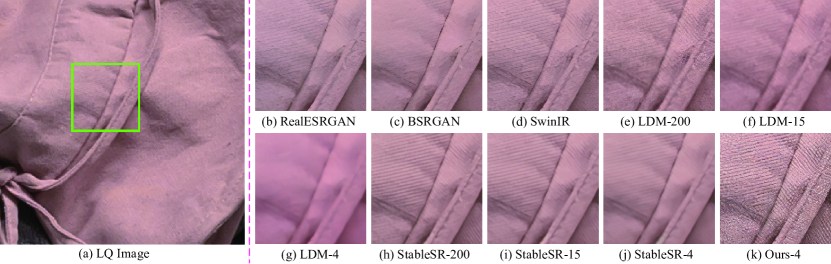
Figure 1: Qualitative comparisons on one typical real-world example of the proposed method and recent state of the arts, including RealESRGAN [38], BSRGAN [39], SwinIR [40], LDM [25], and StableSR [29]. As for the diffusion-based approaches, namely LDM, StableSR, and our proposed method, we annotate the number of sampling steps with the format of “Method-A” for more intuitive visualization, where “A” denotes the number of sampling steps. Note that LDM and StableSR both contain 1000 diffusion steps in training and are accelerated to “A” steps using DDIM [36] during inference. Please zoom in for a better view.

Following the aforementioned motivation, we propose an efficient diffusion model involving a shorter Markov chain for the transition between the HQ image and its corresponding LQ one. The initial state of the Markov chain converges towards an approximate distribution of the HQ image, while the final state converges towards an approximate distribution of the LQ image. To achieve this, we carefully design a transition kernel that gradually shifts the residual information between the HQ/LQ image pair. This approach exhibits superior efficiency in comparison to existing diffusion-based IR methods, given its ability to expeditiously transfer the residual information in several steps. Moreover, our design also allows for an analytical and concise expression for the evidence lower bound, thereby simplifying the formulation of the optimization objective for training purposes. Building upon the constructed diffusion kernel, we further develop a highly flexible noise schedule that controls the speed of residual shifting and the strength of the added noise in each step. This schedule facilitates a fidelity-realism trade-off of the recovered results by tuning its hyper-parameters.

In summary, the main contributions of this work are as follows:

• We propose an efficient diffusion model specifically for IR. It builds up a short Markov chain between the HQ/LQ images, rendering a fast reverse sampling trajectory during inference. Extensive experiments show that our approach requires only four sampling steps to achieve appealing results, outperforming or at least being comparable to current state-of-the-art methods. A preview of the comparison results of the proposed method to recent approaches is shown in Fig. 1.

• A highly flexible noise schedule is designed for the proposed diffusion model, capable of controlling the transition properties more precisely, including the shifting speed and the noise level. Through tuning the hyper-parameters, our method offers a more graceful solution to the widely acknowledged perception-distortion trade-off in IR.

• The proposed method is a general diffusion-based framework for IR, being able to handle various IR tasks. This study has thoroughly substantiated its effectiveness and superiority on three typical and challenging IR tasks, namely image super-resolution, image inpainting, and blind face restoration.

In summary, this work endeavors to formulate an efficient diffusion model customized for IR, with the intention of breaking down the limitation of prevailing approaches on inference efficiency. A preliminary version of this work has been published in NeurIPS 2023 [41], focusing only on the task of image super-resolution. This study makes substantial improvements in both model design and empirical evaluation across diverse IR tasks compared with the conference version. Concretely, we incorporate the perceptual loss into the model optimization and substitute the self-attention layer with Swin transformer in the network architecture. The former modification can further reduce the diffusion steps from 15 to 4, and the latter endows our model with graceful adaptability to handle arbitrary resolutions during inference.

The remainder of the manuscript is organized as follows: Sec. II introduces the related work. Sec. III presents our designed diffusion model for IR. In Sec. IV and Sec. V, extensive experiments are conducted to evaluate the performance of our proposed method on the task of image super-resolution and image inpainting, respectively. Sec. VI finally concludes the paper.

II Related Work

In this section, we briefly review the literature on image restoration, traversing from conventional non-diffusion methodologies to recent diffusion-based approaches.

II-A Conventional Image Restoration Approaches

Most of the conventional IR methods can be cast into the Maximum a Posteriori (MAP) framework, a Bayesian paradigm encompassing a likelihood (loss) term and a prior (regularization) term. The likelihood reflects the underlying noise distribution of the LQ image. The commonly used $L_{2}$ or $L_{1}$ loss indeed corresponds to a Gaussian or Laplacian assumption on image noise. To more accurately depict the noise distribution, some robust alternatives were introduced, such as Poissonian-Gaussian [42], MoG [43], MoEP [44], Dirichlet MoG [45, 46] and so on. Simultaneously, there has been an increased focus on employing image priors to address the inherent ill-posedness of IR over recent decades. Typical image priors encompass total variation [47], wavelet coring [48], non-local similarity [49, 3], sparsity [50, 51], low-rankness [1, 52], dark channel [53, 54], among others. These conventional methods are mainly limited by the model capacity and the subjectivity inherited from the manually designed assumptions on image noise and prior.

In recent years, the landscape of IR has been dominated by deep learning (DL)-based methodologies. The seminal works [4, 55, 2] proposed to solve the IR problem using a convolution neural network, outperforming traditional model-based methods on the tasks of image denoising, super-resolution, and deblurring. Then, many studies [56, 57, 58, 59, 60, 61, 62, 63, 64, 6] have emerged, mainly concentrating on designing more delicate network architectures to further improve the restoration performance. Besides, there have been some discernible investigations that seek to combine current DL tools and classical IR modeling ideas. Notable works include the plug-and play or unfolding paradigm [65, 66, 67], learnable image priors [68, 69, 70, 71], and the loss-oriented methods [72, 73, 74]. The infusion of deep neural networks, owing to their large model capacity, has substantively extended the frontiers of IR tasks.

II-B Diffusion-based Image Restoration Approaches

Inspired by principles from non-equilibrium statistical physics, Sohl-Dickstein et al. [7] proposed the diffusion model to fit complex distributions. Subsequent advancements by Ho et al. [8] and Song et al. [20] further improve its theoretical foundation by integrating denoising score matching and stochastic differential equation, thereby achieving impressive success in image generation [25]. Owing to its powerful generative capability, diffusion models have also found successful applications in the field of IR. Next, we provide a comprehensive overview of recent developments in diffusion-based IR methods.

The most straightforward solution to solve the IR problem using diffusion models is to introduce the LQ image as an addition condition in each timestep. Pioneering this approach, Saharia et al. [23] have successfully trained a diffusion model for image super-resolution. Subsequent studies [21, 14, 27] further expanded upon this approach, exploring its applicability in image deblurring, colorization, and denoising. To circumvent the resource-intensive process of training from scratch, an alternative strategy involves harnessing a pre-trained diffusion model to facilitate IR tasks. Numerous investigations, such as [18, 24, 28, 17, 32, 33, 15], reformulated the reverse sampling procedure of a pre-trained diffusion model into an optimization problem by incorporating the degradation model, enabling solving the IR problem in a zero-shot manner. Most of these methods, however, cannot deal with the blind IR problem, as they rely on a pre-defined degradation model. In contrast, some other works [29, 75, 30] directly introduced a trainable module that takes the LQ image as input. This module modulates the feature maps of the pre-trained diffusion model, steering it toward the direction of generating a desirable HQ image. Such a paradigm eliminates the reliance on a degradation model in the test phase, rendering it capable of handling the blind IR tasks.

The methodologies mentioned above are grounded in the foundational diffusion model initially crafted for image generation, necessitating a large number of sampling steps. This inefficiency presents a constraint on their application in real scenarios. The primary goal of our investigation is to devise a new diffusion model customized for IR, which facilitates a swift transition between the LQ/HQ image pair, thereby enhancing efficiency during inference.

III Methodology

In this section, we present our proposed diffusion model tailored for IR. For ease of presentation, the LQ image and the corresponding HQ image are denoted as $\bm{y}_{0}$ and $\bm{x}_{0}$, respectively. Notably, we further assume $\bm{y}_{0}$ and $\bm{x}_{0}$ have identical spatial resolution, which can be easily achieved by pre-upsampling the LQ image $\bm{y}_{0}$ using nearest neighbor interpolation if necessary.

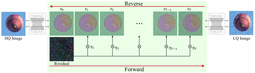
Figure 2: Overview of the proposed method. Our method builds up a Markov chain between the HQ/LQ image pair by shifting their residuals. To alleviate the computational burden of this transition, it can be optionally moved to the latent space of VQGAN [76].

III-A Model Design

The iterative sampling paradigm of diffusion models has proven highly effective in generating intricate and vivid image details, inspiring us to design an iterative approach to address the IR problem as well. Our proposed method builds up a Markov chain to facilitate a transition from the HQ image to its LQ counterpart as shown in Fig. 2. In this way, the restoration of the desirable HQ image can be achieved by sampling along the reverse trajectory of this Markov chain that starts at the given LQ image. Next, we will detail how to construct such a Markov chain specifically for IR.

Forward Process. Let’s denote the residual between the LQ image and its corresponding HQ counterpart as $\bm{e}_{0}$, i.e., $\bm{e}_{0}=\bm{y}_{0}-\bm{x}_{0}$. Our core idea is to construct a transition from $\bm{x}_{0}$ to $\bm{y}_{0}$ by gradually shifting their residual $\bm{e}_{0}$ through a Markov chain with length $T$. Before that, we first introduce a shifting sequence $\{\eta_{t}\}_{t=1}^{T}$, which increases monotonically with respect to timestep $t$ and adheres to the condition of $\eta_{1}\to 0$ and $\eta_{T}\to 1$. Then, the transition distribution is formulated based on this shifting sequence as follows:

$$q(\bm{x}_{t}|\bm{x}_{t-1},\bm{y}_{0})=\mathcal{N}(\bm{x}_{t};\bm{x}_{t-1}+\alpha_{t}\bm{e}_{0},\kappa^{2}\alpha_{t}\bm{I}),~{}t=1,\cdots,T,$$ (1)

where $\alpha_{1}=\eta_{1}$ and $\alpha_{t}=\eta_{t}-\eta_{t-1}$ for $t>1$, $\kappa$ is a hyper-parameter controlling the noise variance, $\bm{I}$ is the identity matrix. Notably, we show that the marginal distribution at any timestep $t$ is analytically integrable, namely

$$q(\bm{x}_{t}|\bm{x}_{0},\bm{y}_{0})=\mathcal{N}(\bm{x}_{t};\bm{x}_{0}+\eta_{t}\bm{e}_{0},\kappa^{2}\eta_{t}\bm{I}),~{}t=1,\cdots,T.$$ (2)

The design of the transition distribution presented in Eq. (1) is guided by two primary principles. The first principle concerns the standard deviation, i.e., $\kappa\sqrt{\alpha_{t}}$, which aims to facilitate a smooth transition between $\bm{x}_{t}$ and $\bm{x}_{t-1}$. This is achieved by bounding the expected distance between $\bm{x}_{t}$ and $\bm{x}_{t-1}$ with $\sqrt{\alpha_{t}}$, given that the image data falls within the range of $[0,1]$. Mathematically, this is expressed as:

$$\text{max}[(\bm{x}_{0}+\eta_{t}\bm{e}_{0})-(\bm{x}_{0}+\eta_{t-1}\bm{e}_{0})]=\text{max}[\alpha_{t}\bm{e}_{0}]<\alpha_{t}<\sqrt{\alpha_{t}},$$ (3)

where $\text{max}[\cdot]$ represents the pixel-wise maximizing operation. The hyper-parameter $\kappa$ is introduced to increase the flexibility of this design. The second principle pertains to the mean parameter, i.e., $\bm{x}_{0}+\alpha_{t}\bm{e}_{0}$. Combining with the definition of $\alpha_{t}$, namely $\alpha_{t}=\eta_{t}-\eta_{t-1}$, it induces the marginal distribution in Eq. (2). Furthermore, the marginal distributions of $\bm{x}_{1}$ and $\bm{x}_{T}$ converges to $\delta_{\bm{x}_{0}}(\bm{x})$ and $\mathcal{N}(\bm{x};\bm{y}_{0},\kappa^{2}\bm{I})$, respectively, serving as approximations for the HQ image and the LQ image. By constructing the Markov chain in such a thoughtful way, it is possible to handle the IR task by inversely sampling from it given the LQ image $\bm{y}_{0}$.

Reverse Process. The reverse process endeavors to estimate the posterior distribution $p(\bm{x}_{0}|\bm{y}_{0})$ through the following formalization:

$$p(\bm{x}_{0}|\bm{y}_{0})=\int p(\bm{x}_{T}|\bm{y}_{0})\prod_{t=1}^{T}p_{\bm{\theta}}(\bm{x}_{t-1}|\bm{x}_{t},\bm{y}_{0})\mathrm{d}\bm{x}_{1:T},$$ (4)

where $p(\bm{x}_{T}|\bm{y}_{0})\approx\mathcal{N}(\bm{x}_{T}|\bm{y}_{0},\kappa^{2}\bm{I})$, $p_{\bm{\theta}}(\bm{x}_{t-1}|\bm{x}_{t},\bm{y}_{0})$ represents the desirable inverse transition kernel from $\bm{x}_{t}$ to $\bm{x}_{t-1}$, parameterized by a learnable parameter $\bm{\theta}$. Consistent with prevalent literature of diffusion model [7, 8, 20], we adopt the following Gaussian assumption:

$$p_{\bm{\theta}}(\bm{x}_{t-1}|\bm{x}_{t},\bm{y}_{0})=\mathcal{N}\left(\bm{x}_{t-1};\bm{\mu}_{\bm{\theta}}(\bm{x}_{t},\bm{y}_{0},t),\bm{\Sigma}_{\bm{\theta}}(\bm{x}_{t},\bm{y}_{0},t)\right).$$ (5)

The optimization for $\bm{\theta}$ is achieved by minimizing the negative evidence lower bound, namely,

$$\min_{\bm{\theta}}\sum_{t}D_{\text{KL}}\left[q(\bm{x}_{t-1}|\bm{x}_{t},\bm{x}_{0},\bm{y}_{0})\|p_{\bm{\theta}}(\bm{x}_{t-1}|\bm{x}_{t},\bm{y}_{0})\right],$$ (6)

where $D_{\text{KL}}[\cdot\|\cdot]$ denotes the Kullback-Leibler (KL) divergence. More mathematical details can be found in [7] or [8].

By combining Eq. (1) and Eq. (2), the target distribution $q(\bm{x}_{t-1}|\bm{x}_{t},\bm{x}_{0},\bm{y}_{0})$ in Eq. (6) can be rendered tractable and expressed in an explicit form given below:

$$q(\bm{x}_{t-1}|\bm{x}_{t},\bm{x}_{0},\bm{y}_{0})=\mathcal{N}\left(\bm{x}_{t-1}\bigg{|}\frac{\eta_{t-1}}{\eta_{t}}\bm{x}_{t}+\frac{\alpha_{t}}{\eta_{t}}\bm{x}_{0},\kappa^{2}\frac{\eta_{t-1}}{\eta_{t}}\alpha_{t}\bm{I}\right).$$ (7)

The detailed calculation of this derivation can be found in Appendix -A. Considering that the variance parameter is independent of $\bm{x}_{t}$ and $\bm{y}_{0}$, we thus set it to be the true variance, i.e.,

$$\bm{\Sigma}_{\bm{\theta}}(\bm{x}_{t},\bm{y}_{0},t)=\kappa^{2}\frac{\eta_{t-1}}{\eta_{t}}\alpha_{t}\bm{I}.$$ (8)

The mean parameter $\bm{\mu}_{\bm{\theta}}(\bm{x}_{t},\bm{y}_{0},t)$ is reparameterized as:

$$\bm{\mu}_{\bm{\theta}}(\bm{x}_{t},\bm{y}_{0},t)=\frac{\eta_{t-1}}{\eta_{t}}\bm{x}_{t}+\frac{\alpha_{t}}{\eta_{t}}f_{\bm{\theta}}(\bm{x}_{t},\bm{y}_{0},t),$$ (9)

where $f_{\bm{\theta}}(\cdot)$ is a deep neural network with parameter $\bm{\theta}$, aiming to predict $\bm{x}_{0}$. We explored different parameterization forms on $\bm{\mu}_{\theta}$ and found that Eq. (9) exhibits superior stability and performance.

Based on Eq. (9), the objective function in Eq. (6) is then simplified as:

$$\min_{\bm{\theta}}\sum\nolimits_{t}w_{t}\|f_{\bm{\theta}}(\bm{x}_{t},\bm{y}_{0},t)-\bm{x}_{0}\|_{2}^{2},$$ (10)

where $w_{t}=\frac{\alpha_{t}}{2\kappa^{2}\eta_{t}\eta_{t-1}}$. In practice, we empirically find that the omission of weight $w_{t}$ results in a notable performance improvement, aligning with the conclusion in [8].

Perceptual Regularization. As presented above, our proposed method facilitates an iterative restoration process starting from the LQ image, in contrast to prior methods that initialize from Gaussian noise. This approach effectively reduces the number of diffusion steps. A comprehensive experimental analysis in Sec. IV-B substantiates that our method yields promising results with a mere 15 sampling steps, demonstrating a notable acceleration compared to established methodologies [25, 29].

Unfortunately, attempts at further acceleration, particularly with fewer than 5 sampling steps, tend to produce over-smooth results. This phenomenon is primarily attributed to that the $L_{2}$-based loss in Eq. (10) favors the prediction of an average over plausible solutions. To overcome this limitation, we introduce the perceptual regularization [77] to impose an additional constraint on the solution space, namely,

$$\min_{\bm{\theta}}\sum\nolimits_{t}\|f_{\bm{\theta}}(\bm{x}_{t},\bm{y}_{0},t)-\bm{x}_{0}\|_{2}^{2}+\lambda l_{p}\left(f_{\bm{\theta}}(\bm{x}_{t},\bm{y}_{0},t),\bm{x}_{0}\right),$$ (11)

where $l_{p}(\cdot,\cdot)$ denotes the pre-trained LPIPS metric, $\lambda$ is a hyper-parameter controlling the relative importance of these two constraints. This simple solution effectively curtails the sampling trajectory to fewer steps, e.g., 4 steps in this study, as shown in Sec. IV-B, while concurrently maintaining superior performance.

Extension to Latent Space. To alleviate the computational overhead in training, our proposed model can be optionally moved into the latent space of VQGAN [76], where the original image is compressed by a factor of four in spatial dimensions. This does not require any modifications on our model other than substituting $\bm{x_{0}}$ and $\bm{y}_{0}$ with their latent codes. An intuitive illustration is shown in Fig. 2.

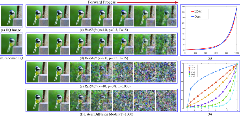
Figure 3: Illustration of the proposed noise schedule. (a) HQ image. (b) Zoomed LQ image. (c)-(d) Diffused images of the proposed noise schedule in timesteps of 1, 3, 5, 7, 9, 12, and 15 under different values of $\kappa$ by fixing $p=0.3$ and $T=15$. (e)-(f) Diffused images of our method with a specified configuration of $\kappa=40,p=0.8,T=1000$ and LDM [25] in timesteps of 100, 200, 400, 600, 800, 900, and 1000. (g) The relative noise intensity (vertical axes, measured by $\sqrt{\nicefrac{{1}}{{\lambda_{\text{snr}}}}}$, where $\lambda_{\text{snr}}$ denotes the signal-to-noise ratio) of the schedules in (d) and (e) w.r.t. the timesteps (horizontal axes). (h) The shifting speed $\sqrt{\eta_{t}}$ (vertical axes) w.r.t. to the timesteps (horizontal axes) across various configurations of $p$. Note that the diffusion processes in this figure are implemented in the latent space, but we display the intermediate results after decoding back to the image space for the purpose of easy visualization.

III-B Noise Schedule

The proposed method employs a hyper-parameter $\kappa$ and a shifting sequence $\{\eta_{t}\}_{t=1}^{T}$ to determine the noise schedule of the diffusion process. In particular, the hyper-parameter $\kappa$ regulates the overall noise intensity during the transition, and its influence on performance is empirically discussed in Sec. IV-B. The subsequent exposition mainly revolves around the construction of the shifting sequence $\{\eta_{t}\}_{t=1}^{T}$.

Equation (2) indicates that the stochastic perturbation in state $\bm{x}_{t}$ is proportional to $\sqrt{\eta_{t}}$, incorporating a scaling factor $\kappa$. This observation motivates us to focus on the design of $\sqrt{\eta_{t}}$ rather than $\eta_{t}$. Previous work by Song et al. [78] has suggested that maintaining a sufficiently small value for $\kappa\sqrt{\eta_{1}}$, such as 0.04 in LDM [25], is imperative to ensure $q(\bm{x}_{1}|\bm{x}_{0},\bm{y}_{0})\approx q(\bm{x}_{0})$. Further considering $\eta_{1}\to 0$, we set $\eta_{1}$ to be the minimum value between $(\nicefrac{{0.04}}{{\kappa}})^{2}$ and $0.001$. For the terminal step $T$, we set $\eta_{T}$ as 0.999, guaranteeing $\eta_{T}\to 1$. For the intermediate timesteps $t\in[2,T-1]$, we propose a non-uniform geometric schedule for $\sqrt{\eta_{t}}$ as follows:

$$\sqrt{\eta_{t}}=\sqrt{\eta_{1}}\times b_{0}^{\beta_{t}},~{}t=2,\cdots,T-1,$$ (12)

where

$$\beta_{t} =\left(\frac{t-1}{T-1}\right)^{p}\times(T-1),$$ (13a)

$$b_{0} =\exp\left[\frac{1}{2(T-1)}\log{\frac{\eta_{T}}{\eta_{1}}}\right].$$ (13b)

It should be noted that the choice of $\beta_{t}$ and $b_{0}$ is grounded in the assumption of $\beta_{1}=0$, $\beta_{T}=T-1$, and $\sqrt{\eta_{T}}=\sqrt{\eta_{1}}\times b_{0}^{T-1}$. The hyper-parameter $p$ controls the growth rate of $\sqrt{\eta_{t}}$, as depicted in Fig. 3(h).

The proposed noise schedule exhibits a high degree of flexibility in three key aspects. First, in the case of small values of $\kappa$, the final state $\bm{x}_{T}$ converges towards a perturbation around the LR image, as illustrated in Fig. 3(c)-(d). Compared to the diffusion process ended at Gaussian noise, this design significantly shortens the length of the Markov chain, thereby improving the inference efficiency. Second, the hyper-parameter $p$ provides precise control over the shifting speed, enabling a fidelity-realism trade-off in the SR results as analyzed in Sec. IV-B. Third, by setting $\kappa=40$ and $p=0.8$, our method achieves a diffusion process that remarkably resembles to LDM [25]. This is clearly demonstrated by the visual results of the diffusion process presented in Fig. 3(e)-(f), and further supported by the comparisons on the relative noise strength as shown in Fig. 3(g).

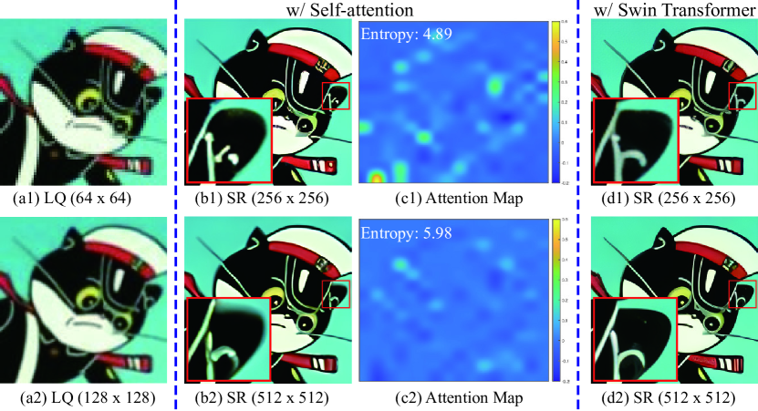
Figure 4: Visual comparison of two different models containing some self-attention layers (denoted as model-1) or Swin transformers (denoted as model-2). (a1) and (a2): zoomed LQ images with resolutions of $64\times 64$ or $128\times 128$. (b1) and (b2): super-resolved results by model-1. (c1) and (c2): visualized attention maps extracted from the first self-attention layer of model-1. Note that these visualized results are obtained by first calculating the first principal component of the attention map via PCA and then reshaping it to the targeted size. In the left-upper corner, we annotate the average entropy values of these attention maps. (d1) and (d2): super-resolved results by model-2.

@articleliang2024control, title=Control Color: Multimodal Diffusion-based Interactive Image Colorization, author=Liang, Zhexin and Li, Zhaochen and Zhou, Shangchen and Li, Chongyi and Loy, Chen Change, journal=arXiv preprint arXiv:2402.10855, year=2024

III-C Discussion on Arbitrary Resolution

It is widely acknowledged that the self-attention layer [79], a pivotal component in recent diffusion architectures, plays a crucial role in capturing global information in image generation. In the field of IR, however, it causes a blurring issue in handling the test images with arbitrary resolutions, particularly when the test resolution largely diverges from the training resolution. One typical example is provided in Figure 4, considering two LQ images with different resolutions. The baseline model with multiple self-attention layers, which is trained on a resolution of $64\times 64$, performs well when the LQ image aligns with the training resolution but yields blurred results when confronted with a mismatched resolution of $128\times 128$.

To analyze the underlying reason, we visualize the attention maps extracted from the first attention layer in this baseline network, as shown in Fig. 4(c1) and (c2). Note that these two attention maps are both interpolated to the resolution of $256\times 256$ for ease of comparison. Evidently, the example with a larger resolution tends to generate a more uniformly distributed attention map, i.e., Fig. 4(c2), being consistent with the entropy values annotated on the left-upper corner. Consequently, a uniformly distributed attention map often leads to an over-smooth outcome, introducing undesirable distortions in performance.

To address this issue, some recent studies [14, 12] have chosen to discard the self-attention layers, a strategy that typically results in a noticeable decline in performance. Inspired by Liang et al. [40], we propose a solution by substituting the self-attention layer with that in Swin Transformer [80]. This straightforward replacement not only alleviates the blurring problem but also maintains the promised performance, as shown in Fig. 4(d1) and (d2). This is because the Swin Transformer computes the attention map in a local window, thus being independent of the image resolution.

IV Experiments on Image Super-resolution

This section offers an evaluation of the proposed method on the task of image super-resolution (SR), with a particular focus on the setting of $\times 4$ SR following existing studies [39, 38]. We first provide an in-depth analysis on the proposed model and then conduct a thorough comparison against recent state-of-the-art methods (SotAs) on one synthetic and two real-world datasets. For the sake of brevity in presentation, our method is herein referred to ResShift or ResShiftL. The former is trained based on the primary loss of diffusion model in Eq. (10), while the latter further introduces the perceptual regularization as shown in Eq. (11). To facilitate a more profound understanding of our designed diffusion model and the noise schedule, the model analysis part of Sec. IV-B mainly centers around ResShift.

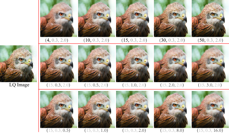
Figure 5: Qualitative comparisons of ResShift under different combinations of ($T$, $p$, $\kappa$) on the task of image super-resolution. For example, “(15, 0.3, 2.0)” represents the recovered result with $T=15$, $p=0.3$, and $\kappa=2.0$. Please zoom in for a better view.

TABLE I: Performance comparison of ResShift on the ImageNet-Test dataset for image super-resolution under different configurations.

Configurations			Metrics
$T$	$p$	$\kappa$	PSNR$\uparrow$	SSIM$\uparrow$	LPIPS$\downarrow$
4	0.3	2.0	25.64	0.6903	0.3242
10			25.20	0.6828	0.2517
15			25.01	0.6769	0.2312
30			24.52	0.6585	0.2253
50			24.22	0.6483	0.2212
15	0.3	2.0	25.01	0.6769	0.2312
	0.5		25.05	0.6745	0.2387
	1.0		25.12	0.6780	0.2613
	2.0		25.32	0.6827	0.3050
	3.0		25.39	0.5813	0.3432
15	0.3	0.5	24.90	0.6709	0.2437
		1.0	24.84	0.6699	0.2354
		2.0	25.01	0.6769	0.2312
		8.0	25.31	0.6858	0.2592
		16.0	24.46	0.6891	0.2772

IV-A Experimental Setup

Training Details. The HQ images in our training data, with a resolution of $256\times 256$, are randomly cropped from the training set of ImageNet [81] like LDM [25]. The LQ images are synthesized using the degradation pipeline of RealESRGAN [38]. To train our model, we adopted the Adam [82] algorithm with its default settings in PyTorch [83] and set the mini-batch size as 64. The learning rate is gradually decayed from $5\text{e-}5$ to $2\text{e-}5$ according to the annealing cosine schedule [84], and a total of 500K iterations are implemented throughout the training. As for the network architecture, the UNet backbone in DDPM [8] is employed. To increase our model’s adaptability to arbitrary image resolutions, we replace the self-attention layer in UNet with Swin Transformer [80] as explained in Sec. III-C.

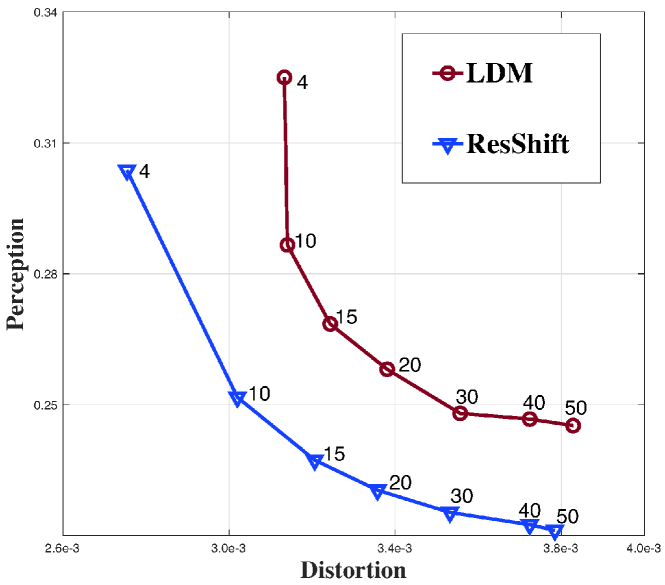
Figure 6: Perception-distortion trade-off of ResShift and LDM. The vertical and horizontal axes represent the strength of the perception and distortion, measured by LPIPS and MSE, respectively.

Test Datasets. We randomly select 3000 images from the validation set of ImageNet [81] as our synthetic test data, denoted as ImageNet-Test for convenience. The LQ images are generated based on the commonly-used degradation model:

$$\bm{y}=(\bm{x}*\bm{k})\downarrow+\bm{n},$$ (14)

where $\bm{k}$ is the blurring kernel, $\bm{n}$ is the noise, $\bm{y}$ and $\bm{x}$ denote the LQ image and HQ image, respectively. To comprehensively evaluate the performance of our model, we consider more complicated types of blurring kernel, downsampling operator, and noise type. The detailed settings on them can be found in Appendix -C1. It should be noted that we select the HQ images from ImageNet [81] instead of the prevailing datasets in SR, such as Set5 [85], Set14 [86], and Urban100 [87]. The rationale behind this setting is rooted in the fact that these prevailing datasets only contain very few source images, which fail to thoroughly evaluate the performance of various methods under a multitude of different degradation types.

Two real-world datasets are adopted to evaluate the efficacy of our method. The first is RealSR-V3 [88], containing 100 real images captured by Canon 5D3 and Nikon D810 cameras. Additionally, we collect another real-world dataset named RealSet80. It comprises 50 LR images widely used in recent literature [89, 90, 91, 92, 38, 93]. The remaining 30 images are downloaded from the internet by ourselves.

TABLE II: Quantitative comparison on performance, running time, and the number of parameters of different methods on ImageNet-Test dataset for Image Super-resolution. The results of the diffusion-based methods are denoted as “Method-A”, where “A” represents the number of sampling steps. Running time is tested on NVIDIA Tesla A100 GPU on the x4 (64$\rightarrow$256) SR task. The best and second best results are highlighted in bold and underline. The non-trainable parameters, such as the parameters of VQGAN in LDM, are marked with gray color for clarity.

Methods	Metrics
6
	PSNR$\uparrow$	SSIM$\uparrow$	LPIPS$\downarrow$	Runtime (s)	#Params (M)
ESRGAN [72]	20.67	0.448	0.485	0.038	16.70
RealSR-JPEG [94]	23.11	0.591	0.326	0.038	16.70
BSRGAN [39]	24.42	0.659	0.259	0.038	16.70
SwinIR [40]	23.99	0.667	0.238	0.107	28.01
RealESRGAN [38]	24.04	0.665	0.254	0.038	16.70
DASR [95]	24.75	0.675	0.250	0.022	8.06
LDM-15 [25]	24.89	0.670	0.269	0.247	113.60+55.32
LDM-4 [25]	24.74	0.657	0.345	0.077
StableSR-15 [29]	23.37	0.631	0.262	1.070	52.49+1422.49
StableSR-4 [29]	24.11	0.658	0.287	0.399
ResShift-15	25.01	0.677	0.231	0.682	118.59+55.32
ResShiftL-4	25.02	0.683	0.208	0.186

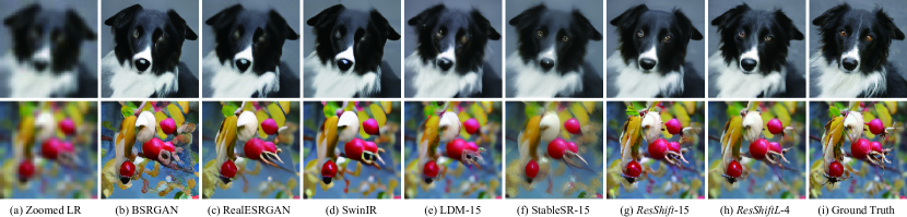
Figure 7: Qualitative results of different methods on the synthetic ImageNet-Test dataset for image super-resolution. Note that we only display the comparison results to the recent five SotA methods in (b)-(f) due to the page limitation, and the whole results can be found in Fig. 14 of the appendix. Please zoom in for a better view.

TABLE III: Quantitative results of different methods on two real-world datasets for image super-resolution. Note that the results of diffusion-based methods are denoted as “Method-A”, where “A” represents the number of sampling steps. The best and second best results are highlighted in bold and underline.

Methods	Datasets
5
	RealSR-V3 [88]		RealSet80
5
	CLIPIQA$\uparrow$	MUSIQ$\uparrow$	CLIPIQA$\uparrow$	MUSIQ$\uparrow$
ESRGAN [72]	0.2362	29.048	0.4165	48.153
RealSR-JPEG [94]	0.3615	36.076	0.5828	57.379
BSRGAN [39]	0.5439	63.586	0.6263	66.629
SwinIR [40]	0.4654	59.632	0.6072	64.739
RealESRGAN [38]	0.4898	59.678	0.6189	64.496
DASR [95]	0.3629	45.825	0.5311	58.974
LDM-50 [25]	0.4907	54.391	0.5511	55.826
LDM-15 [25]	0.3836	49.317	0.4592	50.972
StableSR-50 [29]	0.5208	60.177	0.6214	62.761
StableSR-15 [29]	0.4974	59.099	0.5975	61.476
ResShift-15	0.6014	58.979	0.6645	62.782
ResShiftL-4	0.5854	56.184	0.6483	61.017

Compared Methods. We evaluate the effectiveness of ResShift and ResShiftL in comparison to seven recent SR methods, namely RealSR-JPEG [94], BSRGAN [39], RealESRGAN [38], SwinIR [40], DASR [95], LDM [25], and StableSR [29]. LDM and StableSR are both diffusion-based methods trained with 1,000 diffusion steps. For a fair comparison, we accelerate them to 15 or 4 steps using the DDIM [36] algorithm during inference in this study. The hyper-parameter $\eta$ in DDIM is set to be 1.0 as this value yields the most realistic results. For clarity, the results of LDM and StableSR are denoted as “Method-A”, where “A” represents the number of inference steps.

Evaluation Metrics. We evaluate the efficacy of different methods using three widely used metrics in most of the SR literature, namely PSNR, SSIM [96], and LPIPS [77], on the synthetic dataset. Notably, PSNR and SSIM are calculated in the luminance (Y) channel of YCbCr space, while LPIPS is directly computed in the standard RGB (sRGB) space. For assessments on real-world datasets, we mainly rely on CLIPIQA [97] and MUSIQ [98] as evaluative metrics to compare the performance of various methods. CLIPIQA and MUSIQ are both non-reference metrics specifically designed for assessing the realism of images. Of particular note, CLIPIQA leverages the CLIP [99] model, pre-trained on the extensive Laion400M [100] dataset, thereby demonstrating strong generalization ability.

IV-B Model Analysis

We analyze the performance of ResShift under different settings with respect to (w.r.t.) the number of diffusion steps $T$ and the hyper-parameters $p$ in Eq. (13a) and $\kappa$ in Eq. (1).

Diffusion Steps $T$ and Hyper-parameter $p$. The proposed transition distribution in Eq. (1) significantly reduces the diffusion steps $T$ in the Markov chain. The hyper-parameter $p$ allows for flexible control over the rate of residual shifting during the transition. Performance evaluations of ResShift on the test dataset of ImageNet-Test, under various configurations of $T$ and $p$, are presented in Table I. This comparison reveals that both $T$ and $p$ render an evident trade-off between the fidelity (measured by the reference metrics of PSNR and SSIM) and the perceptual quality (measured by LPIPS) of the super-resolved results. Taking the hyper-parameter $p$ as an example, an upward adjustment of its value is associated with enhancements in fidelity-oriented metrics while concurrently resulting in a deterioration in perceptual quality. Furthermore, the visual comparison in Fig. 5 shows that a large value of $p$ will suppress the model’s ability to hallucinate more image details, thereby yielding blurry outputs.

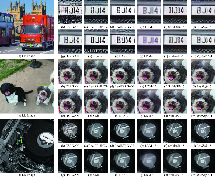
Figure 8: Qualitative comparisons on three real-world examples from RealSet80. Please zoom in for a better view.

Perception-Distortion Trade-off. There exists a well-known phenomenon called perception-distortion trade-off [101] in SR. In particular, the augmentation of the generative capability of a restoration model, such as increasing the sampling steps for a diffusion-based method or amplifying the weight of the adversarial loss for a GAN-based method, will result in a deterioration in fidelity preservation while concurrently enhancing the realism of restored images. In Fig. 6, we plot the perception-distortion curves of ResShift and the representative baseline method LDM [25], wherein the perception and distortion are measured by LPIPS and mean square-error (MSE), respectively. This plot reflects the perception quality and the reconstruction fidelity of ResShift and LDM across varying numbers of diffusion steps from 4 to 50. As can be observed, the perception-distortion curve of ResShift consistently resides beneath that of the LDM, indicating its superiority in balancing perception and distortion.

Hyper-parameter $\kappa$. Equation (2) indicates that $\kappa$ dominates the noise strength in state $\bm{x}_{t}$. In Table I, we report the influence of varying $\kappa$ values on the performance of ResShift. Combining this quantitative comparison with the visualization in Fig. 5, we can find that excessively large or small values of $\kappa$ will smooth the recovered results, regardless of their favorable metrics of PSNR and SSIM. When $\kappa$ is in the range of $[1.0,2.0]$, our method achieves the most realistic quality, as evidenced by LPIPS, which is more desirable in real applications. We thus set $\kappa$ to be $2.0$ in this work.

Perceptual regularization. Considering both of efficiency and performance, we set $T=15$, $\kappa=2$, and $p=0.3$ throughout this study. The model under such a setting is called ResShift following our previous conference paper [46]. To further enhance the inference efficiency, we incorporate an additional perceptual regularizer as shown in Eq. (11), obtaining a more efficient model named ResShiftL with only 4 sampling steps. The detailed quantitative comparison is listed in Table II. Despite the reduction in diffusion steps, ResShiftL still outperforms ResShift across all three metrics, indicating the necessity of the perceptual regularizer. A particularly interesting observation here is that this perceptual constraint not only improves the perceptual quality but also preserves fidelity, as substantiated by the metrics of PSNR and SSIM.

TABLE IV: Quantitative comparisons of various methods on the test dataset ImageNet-Test for inpainting. The best and second best results are highlighted in bold and underline, respectively.

Mask Types	Metrics	Methods
9
		DeepFillv2 [5]	LaMa [6]	RePaint [17]	DDRM [28]	Score-SDE [20]	MCG [24]	ResShiftL
Box	LPIPS$\downarrow$	0.1524	0.1158	0.1498	0.2241	0.2073	0.1464	0.1156
	CLIPIQA$\uparrow$	0.4539	0.4492	0.4586	0.4705	0.4350	0.4639	0.4587
Irregular	LPIPS$\downarrow$	0.2523	0.1959	0.2569	0.3712	0.3350	0.2389	0.1931
	CLIPIQA$\uparrow$	0.4199	0.4204	0.4392	0.4304	0.4131	0.4388	0.4432
Half	LPIPS$\downarrow$	0.3237	0.2925	0.3331	0.4404	0.3709	0.3120	0.2663
	CLIPIQA$\uparrow$	0.4147	0.4183	0.4490	0.4316	0.4263	0.4599	0.4476
Expand	LPIPS$\downarrow$	0.5032	0.3561	0.4957	0.6081	0.5620	0.4320	0.3439
	CLIPIQA$\uparrow$	0.4480	0.4251	0.4530	0.4276	0.4293	0.4611	0.4581
Average	LPIPS$\downarrow$	0.2914	0.2401	0.3089	0.4152	0.3688	0.2823	0.2298
	CLIPIQA$\uparrow$	0.4310	0.4282	0.4499	0.4400	0.4260	0.4559	0.4519

TABLE V: Quantitative comparisons of various methods on the test dataset CelebA-Test for inpainting. The best and second best results are highlighted in bold and underline, respectively.

Mask Types	Metrics	Methods
9
		DeepFillv2 [5]	LaMa [6]	RePaint [17]	DDRM [28]	Score-SDE [20]	MCG [24]	ResShiftL
Box	LPIPS$\downarrow$	0.0719	0.0533	0.0702	0.0755	0.1087	0.0764	0.0550
	CLIPIQA$\uparrow$	0.4487	0.4365	0.4754	0.4521	0.4547	0.4714	0.4915
Irregular	LPIPS$\downarrow$	0.1690	0.1221	0.1602	0.1632	0.2315	0.1522	0.1169
	CLIPIQA$\uparrow$	0.4297	0.4214	0.4558	0.4359	0.4385	0.4649	0.5029
Half	LPIPS$\downarrow$	0.2147	0.1603	0.1936	0.2039	0.2415	0.1853	0.1535
	CLIPIQA$\uparrow$	0.4129	0.4056	0.4751	0.4424	0.4603	0.4772	0.5189
Expand	LPIPS$\downarrow$	0.4003	0.2961	0.3858	0.3978	0.4456	0.3471	0.2772
	CLIPIQA$\uparrow$	0.3989	0.4053	0.4469	0.4280	0.4378	0.5022	0.5111
Average	LPIPS$\downarrow$	0.2140	0.1580	0.2029	0.2101	0.2568	0.1902	0.1506
	CLIPIQA$\uparrow$	0.4225	0.4172	0.4633	0.4396	0.4478	0.4789	0.5061

IV-C Evaluation on Synthetic Data

We present a comparative analysis of the proposed method with recent SotA approaches on the ImageNet-Test dataset, as summarized in Table II and Fig. 7. Based on this evaluation, several significant conclusions can be drawn as follows: i) ResShiftL exhibits superior performance across all three metrics, affirming the effectiveness and superiority of the proposed method. ii) The notably higher PSNR and SSIM values attained by ResShiftL indicate its capacity to better preserve fidelity to ground truth images. This advantage primarily arises from our well-designed diffusion model, which starts from a subtle disturbance of the LQ image, rather than the conventional assumption of white Gaussian noise in LDM [25] and StableSR [29]. iii) Considering the metric of LPIPS, which gauges the perceptual quality and realism of the recovered image, ResShiftL also demonstrates clear superiority over existing methods. In summary, the proposed ResShiftL exhibits remarkable capabilities in generating more realistic results while preserving fidelity.

In addition, Table II also lists the efficiency comparison of different methods. We can easily observe that ResShiftL attains a preeminent equilibrium between performance and efficiency, surpassing recent diffusion-based methods LDM [25] and StableSR [29]. Notably, even in comparison with the SotA GAN-based method SwinIR [40], it still exhibits comparable speed while retaining superior performance.

IV-D Evaluation on Real-World Data

Table III lists the comparative evaluation using CLIPIQA [97] and MUSIQ [98] for various approaches on two real-world datasets, namely RealSR-V3 [88] and RealSet80. Note that CLIPIQA, benefiting from the powerful representative capability inherited from CLIP, performs consistently and robustly in assessing the perceptional quality of natural images. The results in Table III reveal that the proposed ResShift or ResShiftL notably outperforms existing methods in terms of CLIPIQA. This suggests that the restored outputs by our method better align with human visual and perceptive systems. In the case of MUSIQ evaluation, ResShift attains competitive performance when compared to current SotA methods, namely BSRGAN [39], SwinIR [40], and RealESRGAN [38]. Collectively, our method shows promising capability in addressing real-world SR challenges.

We display three real-world examples in Fig. 8. We consider diverse scenarios, including text, animal, and natural images to ensure a comprehensive evaluation. An obvious observation is that ResShift or ResShiftL produces more naturalistic image structures. We note that the recovered results of LDM [25] and StableSR [29] are excessively smooth when compressing the inference steps to match with our proposed method, i.e., 15 or 4 steps, largely deviating from the training procedure’s 1,000 steps. Even though other GAN-based methods may also succeed in hallucinating plausible structures to some extent, they are often accompanied by obvious artifacts.

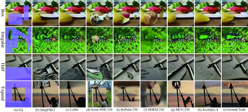
Figure 9: Visual comparisons of various methods on the test dataset of ImageNet-Test for inpainting. The results of diffusion-based methods are denoted as “Method-A”, where “A” represents the number of sampling steps. The masked areas are highlighted using a purple color. Please zoom in for a better view.

V Experiments on Image Inpainting

The proposed diffusion model is a general framework for IR. This section presents a series of experiments to validate its effectiveness in the task of image inpainting. Additional experiments on blind face restoration are provided in the appendix due to page limitation.

V-A Experimental Setup

Training Details. In addressing the task of inpainting, we train two variants of the ResShiftL model, both implemented at a resolution of $256\times 256$. These two variants are tailored for natural images and facial images, respectively. The former model is trained using the training dataset of ImageNet [81], while the latter is trained on the widely used face dataset FFHQ [102]. During training, we randomly generate the image masks to synthesize the LQ images following LaMa [6]. The other training configurations are kept consistent with those in image super-resolution, as detailed in Sec. IV-A.

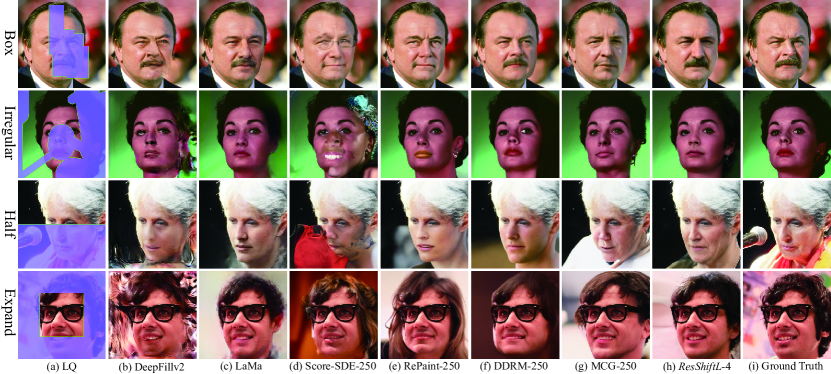
Figure 10: Visual comparisons of various methods on the test dataset of CelebA-Test for inpainting. The results of diffusion-based methods are denoted as “Method-A”, where “A” represents the number of sampling steps. The masked areas are highlighted using a purple color. Please zoom in for a better view.

Test Datasets. Two test datasets are constructed by randomly selecting 2,000 images from the validation dataset of ImageNet [81] and CelebA-HQ [103], to facilitate an assessment on natural images and facial images, respectively. These images in each dataset are uniformly divided into four groups to synthesize different types of masked images. To ensure a thorough evaluation, four distinct mask types, denoted as “Box” mask, “Irregular” mask, “Half” mask, and “Expand” mask, are considered as visually shown in Fig. 9. For each mask type, we randomly generate a set of 500 masks, and then employ them to simulate the LQ images. These two datasets are denoted as ImageNet-Test and CelebA-Test in this section.

Compared Methods. In order to evaluate the efficacy of ResShiftL, a comparative analysis is conducted against two GAN-based methods, including DeepFillv2 [5] and LaMa [6], as well as four diffusion-based methods, namely Score-SDE [20], RePaint [17], DDRM [28], and MCG [24]. For the diffusion-based methods, we accelerate their sampling process to 250 steps using the DDIM [36] algorithm.

Evaluation Metrics. For the sake of comprehensively assessing the performance of various approaches, we adopt one full-reference metric LPIPS [77] and one no-reference metric CLIPIQA [97] as our principal evaluative criteria.

V-B Comparison with SotA Methods

We provide a quantitative evaluation of different methods on the test dataset of ImageNet-Test and CelebA-Test, as detailed in Table IV and Table V, respectively. The proposed ResShiftL achieves the best or, at the very least, comparable performance to recent SotA methods across most cases, particularly excelling in the more challenging mask types such as “Irregular”, “Half”, and “Expand”. In comparison to other diffusion-based approaches, ResShiftL still maintains a competitive advantage, even with a significantly reduced number of sampling steps (4 vs. 250).

A series of visual illustrations on various mask types are displayed in Fig. 9 and Fig. 10. In the case of “Box” mask, recent methods, namely LaMa [6] and MCG [24], and our ResShiftL all perform well. For the other three mask types containing large occluded areas, most of the comparison methods fail to handle such complicated scenarios. In contrast, the proposed ResShiftL consistently yields more plausible and realistic results under these scenarios, especially on the preservation of coherency to the unmasked regions. The qualitative analysis presented herein reaffirms the stability and exceptional performance of ResShiftL, aligning with the quantitative comparison above.

VI Conclusion

In this work, we have introduced an efficient diffusion model specifically designed for IR. Unlike existing diffusion-based IR methods that require a large number of iterations to achieve satisfactory results, our proposed method is capable of formulating a diffusion model with only four sampling steps, thereby significantly improving the efficiency during inference. The core idea is to corrupt the HQ image towards its LQ counterpart instead of the Gaussian white noise. This strategy can effectively truncate the length of the diffusion model. Extensive experiments on the tasks of image super-resolution and image inpainting have demonstrated the superiority of our proposed method. In addition, more discussion on the limitations of the proposed method can be found in Appendix -B2. We believe that our work will pave the way for the development of more efficient and effective diffusion models to address the IR problem.

-A Mathematical Details

• Derivation of Eq. (2): According to the transition distribution of Eq. (1) of our manuscript, $\bm{x}_{t}$ can be sampled via the following reparameterization trick:

  $$\bm{x}_{t}=\bm{x}_{t-1}+\alpha_{t}\bm{e}_{0}+\kappa\sqrt{\alpha_{t}}\bm{\xi}_{t},$$ (15)

  where $\bm{\xi}_{t}\sim\mathcal{N}(\bm{x}|\bm{0},\bm{I})$, $\alpha_{t}=\eta_{t}-\eta_{t-1}$ for $t>1$ and $\alpha_{1}=\eta_{1}$.

  Applying this sampling trick recursively, we can build up the relation between $\bm{x}_{t}$ and $\bm{x}_{0}$ as follows:

  $$\bm{x}_{t} =\bm{x}_{0}+\sum_{i=1}^{t}\alpha_{i}\bm{e}_{0}+\kappa\sum_{i=1}^{t}\sqrt{\alpha_{i}}\bm{\xi}_{i}$$

  $$=\bm{x}_{0}+\eta_{t}\bm{e}_{0}+\kappa\sum_{i=1}^{t}\sqrt{\alpha_{i}}\bm{\xi}_{i},$$ (16)

  where $\bm{\xi}_{i}\sim\mathcal{N}(\bm{x}|\bm{0},\bm{I})$.

  We can further merge $\bm{\xi}_{1},\bm{\xi}_{2},\cdots,\bm{\xi}_{t}$ and simplify Eq. (16) as follows:

  $$\bm{x}_{t}=\bm{x}_{0}+\eta_{t}\bm{e}_{0}+\kappa\sqrt{\eta_{t}}\bm{\xi_{t}}.$$ (17)

  Then the marginal distribution of Eq. (2) in the main text is obtained based on Eq. (17).

• Derivation of Eq. (7): According to Bayes’s theorem, we have

  $$q(\bm{x}_{t-1}|\bm{x}_{t},\bm{x}_{0},\bm{y}_{0})\propto q(\bm{x}_{t}|\bm{x}_{t-1},\bm{y}_{0})q(\bm{x_{t-1}}|\bm{x}_{0},\bm{y}_{0}),$$ (18)

  where

  $$q(\bm{x}_{t}|\bm{x}_{t-1},\bm{y}_{0})=\mathcal{N}(\bm{x}_{t};\bm{x}_{t-1}+\alpha_{t}\bm{e}_{0},\kappa^{2}\alpha_{t}\bm{I}),$$

  $$q(\bm{x_{t-1}}|\bm{x}_{0},\bm{y}_{0})=\mathcal{N}(\bm{x}_{t-1};\bm{x}_{0}+\eta_{t-1}\bm{e}_{0},\kappa^{2}\eta_{t-1}\bm{I}).$$ (19)

  We now focus on the quadratic form in the exponent of $q(\bm{x}_{t-1}|\bm{x}_{t},\bm{x}_{0},\bm{y}_{0})$, namely,

  $$\mathrel{\phantom{=}}-\frac{(\bm{x}_{t}-\bm{x}_{t-1}-\alpha_{t}\bm{e}_{0})(\bm{x}_{t}-\bm{x}_{t-1}-\alpha_{t}\bm{e}_{0})^{T}}{2\kappa^{2}\alpha_{t}}-\frac{(\bm{x}_{t-1}-\bm{x}_{0}-\eta_{t-1}\bm{e}_{0})(\bm{x}_{t-1}-\bm{x}_{0}-\eta_{t-1}\bm{e}_{0})^{T}}{2\kappa^{2}\eta_{t-1}}$$

  $$=-\frac{1}{2}\left[\frac{1}{\kappa^{2}\alpha_{t}}+\frac{1}{\kappa^{2}\eta_{t-1}}\right]\bm{x}_{t-1}\bm{x}_{t-1}^{T}+\left[\frac{\bm{x}_{t}-\alpha_{t}\bm{e}_{0}}{\kappa^{2}\alpha_{t}}+\frac{\bm{x}_{0}+\eta_{t-1}\bm{e}_{0}}{\kappa^{2}\eta_{t-1}}\right]\bm{x}_{t-1}^{T}+\text{const}$$

  $$=-\frac{(\bm{x}_{t-1}-\bm{\mu})(\bm{x}_{t-1}-\bm{\mu})^{T}}{2\lambda^{2}}+\text{const}$$ (20)

  where

  $$\bm{\mu}=\frac{\eta_{t-1}}{\eta_{t}}\bm{x}_{t}+\frac{\alpha_{t}}{\eta_{t}}\bm{x}_{0},~{}\lambda^{2}=\kappa^{2}\frac{\eta_{t-1}}{\eta_{t}}\alpha_{t},$$ (21)

  and const denotes the item that is independent of $\bm{x}_{t-1}$. This quadratic form induces the Gaussian distribution of Eq. (7) in our manuscript.

-B Experimental Results on Image Super-resolution

-B1 Degradation Settings of the Synthetic Dataset

We synthesize the testing dataset ImageNet-Test based on the degradation model in RealESRGAN [38] but remove the second-order operation. We observed that the low-quality (LQ) image generated by the pipeline with second-order degradation exhibited significantly more pronounced corruption than most of the real-world LQ images, we thus discarded the second-order operation to align the authentic degradation better. Next, we gave the detailed configuration of the blurring kernel, downsampling operator, and noise types.

Blurring kernel. The blurring kernel is randomly sampled from the isotropic Gaussian and anisotropic Gaussian kernels with a probability of [0.6, 0.4]. The window size of the kernel is set to 13. For isotropic Gaussian kernel, the kernel width is uniformly sampled from [0.2, 0.8]. For an anisotropic Gaussian kernel, the kernel widths along the $x$-axis and $y$-axis are both randomly sampled from [0.2, 0.8].

Downampling. We downsample the image using the “interpolate” function of PyTorch [83]. The interpolation mode is randomly selected from “area”, “bilinear”, and “bicubic”.

Noise. We first add Gaussian and Poisson noise with a probability of [0.5, 0.5]. For Gaussian noise, the noise level is randomly chosen from [1,15]. For Poisson noise, we set the scale parameter in [0.05, 0.3]. Finally, the noisy image is further compressed using JPEG with a quality factor ranging in [70, 95].

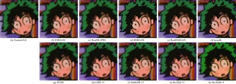
Figure 11: One typical real-world failed case in the task of image super-resolution.

-B2 Limitation

Albeit its overall strong performance, the proposed method occasionally exhibits failures. One such instance is illustrated in Fig. 11, where it cannot produce satisfactory results for a severely degraded comic image. It should be noted that other comparison methods also struggle to address this particular example. This is not an unexpected outcome as most modern image super-resolution (SR) methods are trained on synthetic datasets simulated by manually assumed degradation models [39, 38], which still cannot cover the full range of complicated real degradation types. Therefore, developing a more practical degradation model for SR is an essential avenue for future research.

-C Experimental Results on Blind Face Restoration

-C1 Experimental setup

Training Settings. Our model was trained on the FFHQ dataset [102] that contains 70k high-quality (HQ) face images. We firstly resized the HQ images into a resolution of $512\times 512$, and then synthesized the LQ images following a typical degradation model used in recent literature [104]:

$$\bm{y}=\left\{\left[\left(\bm{x}*\bm{k}_{l}\right)\downarrow_{s}+\bm{n}_{\sigma}\right]_{\text{JPEG}_{q}}\right\}{\uparrow_{s}},$$ (22)

where $\bm{y}$ and $\bm{x}$ are the LQ and HQ image, $\bm{k}_{l}$ is the Gaussian kernel with kernel width $l$, $\bm{n}_{\sigma}$ is Gaussian noise with standard deviation $\sigma$, $*$ is 2D convolutional operator, $\downarrow_{s}$ and $\uparrow_{s}$ are the Bicubic downsampling or upsampling operators with scale $s$, and $[\cdot]_{\text{JPEG}_{q}}$ represents the JPEG compression process with quality factor $q$. And the hyper-parameters $l$, $s$, $\sigma$, and $q$ are uniformly sampled from $[0.1,15]$, $[0.8,32]$, $[0,20]$, and $[30,100]$ respectively. The other training configurations were kept the same as those in image super-resolution.

Testing Datasets. We evaluate ResShiftL on one synthetic dataset and three real-world datasets. The synthetic dataset, denoted as CelebA-Test, contains 2,000 HQ images from CelebA-HQ [103], and the corresponding LQ images are synthesized via Eq. (22). As for the real-world datasets, we consider three typical ones with different degrees of degradation, namely LFW, WebPhoto [104], and WIDER [105]. LFW consists of 1711 mildly degraded face images in the wild, which contains one image for each person in LFW dataset [106]. WebPhoto is made up of 407 face images crawled from the internet. Some of them are old photos with severe degradation. WIDER selects 970 face images with very heavy degradation from the WIDER Face dataset [107], it is thus suitable to test the robustness of different methods under severe degradation.

TABLE VI: Quantitative comparison of different methods on CelebA-Test dataset for blind face restoration. The results of the diffusion-based methods are denoted as “Method-A”, where “A” represents the number of sampling steps. The best and second best results are highlighted in bold and underline.

Methods	Metrics
8
	PSNR$\uparrow$	SSIM$\uparrow$	LPIPS$\downarrow$	IDS$\downarrow$	LMD$\downarrow$	FID-F$\downarrow$	FID-G$\downarrow$
DFDNet [108]	22.97	0.631	0.502	86.32	20.79	92.22	77.10
PSFRGAN [109]	22.58	0.628	0.411	70.32	7.19	65.65	62.44
GFPGAN [104]	22.06	0.629	0.413	68.78	8.64	49.15	56.13
RestoreFormer [110]	22.55	0.598	0.423	65.93	8.20	50.76	53.25
VQFR [111]	21.80	0.579	0.424	67.62	8.46	49.62	57.12
CodeFormer [105]	23.58	0.661	0.324	59.14	5.04	64.25	26.65
DifFace-100 [19]	24.24	0.702	0.334	61.25	5.13	52.34	22.84
ResShiftL-4	23.41	0.671	0.309	59.70	5.05	52.07	17.84

TABLE VII: Quantitative comparison of different methods on three real-world datasets for blind face restoration. The results of the diffusion-based methods are denoted as “Method-A”, where “A” represents the number of sampling steps. The best and second best results are highlighted in bold and underline.

Methods	Datasets
7
	LFW		WebPhoto		WIDER
7
	FID-F$\downarrow$	MUSIQ$\uparrow$	FID-F$\downarrow$	MUSIQ$\uparrow$	FID-F$\downarrow$	MUSIQ$\uparrow$
DFDNet [108]	59.81	73.11	92.39	69.03	57.85	63.21
PSFRGAN [109]	49.65	73.60	85.03	71.67	49.85	71.51
GFPGAN [104]	50.02	73.57	87.57	72.08	39.46	72.82
RestoreFormer [110]	48.50	73.70	78.16	69.84	49.85	67.84
VQFR [111]	44.14	74.02	75.38	72.00	50.79	74.74
CodeFormer [105]	52.43	75.49	83.27	73.99	38.86	73.40
DifFace-100 [19]	45.64	70.39	89.99	66.29	38.40	65.99
ResShiftL-4	52.40	70.68	74.80	70.90	38.12	71.07

Compared Methods. We compare ResShiftL with seven recent BFR methods, including DFDNet [108], PSFRGAN [109], GFPGAN [104], RestoreFormer [110], VQFR [111], CodeFormer [105], and DifFace [19].

Evaluation Metrics. To comprehensively assess various methods, this study adopts six quantitative metrics following the setting of VQFR [111], namely PSNR, SSIM [112], LPIPS [77], identity score (IDS), landmark distance (LMD), and FID [113]. Note that IDS, also referred to as ”Deg” in certain literature [111], and LMD both serve as quantifiers for the identity between the restored images and their ground truths. IDS gauges the embedding angle of ArcFace [114], while LMD calculates the landmark distance using $L_{2}$ norm between pairs of images. FID quantifies the KL divergence between the feature distributions, assumed as Gaussian distribution, of the restored images and a high-quality reference dataset. For the reference dataset, we employ both the ground truth images and the FFHQ [103] dataset. The corresponding results computed under these two settings are denoted as “FID-G” and “FID-F” for clarity. On the real-world datasets, we mainly adopt two no-reference metrics, namely FID-F and MUSIQ [98], since the underlying ground truth images are unavailable.

-C2 Evaluation on Synthetic Dataset

We present the comparative results on CelebA-Test in Table VI. The proposed ResShiftL demonstrates superior performance, particularly in terms of LPIPS and FID-G, indicating the heightened alignment of its restored results with the perceptual system of humans. Regarding the identity-related metrics, namely LMD and IDS, our method attains the second-best rankings, substantiating its powerful capability for identity preservation. Furthermore, our method exhibits, at a minimum, comparable performance to recent state-of-the-art (SotA) techniques across other evaluated metrics. In summary, our proposed method manifests commendable and consistent proficiency in blind face restoration.

For visualization, four typical examples of the CelebA-Test are displayed in Fig. 12. In the first and second examples with mild degradation, most of the comparison methods can restore a realistic-looking image. When confronted with more severe degradation as shown in the third and fourth examples, only CodeFormer [105], DifFace [19], and ResShiftL can handle such cases, yielding satisfactory facial images. However, the results of CodeFormer still contain some slight artifacts in specific areas, such as hair, as highlighted by red arrows in Fig. 12). As for DifFace, it needs 100 sampling steps, largely limiting its efficiency. In contrast, the proposed ResShiftL not only requires much fewer diffusion steps, i.e., 4 steps, but also performs more stably under this challenging degradation setting.

-C3 Evaluation on Real-world Dataset

The comparative results on three real-world datasets are summarized in Table VII. We can observe that ResShiftL surpasses its counterparts with regard to the metric of FID-F, while maintaining comparability with recent SotA methodologies in terms of MUSIQ. To supplement the analysis, we show several typical examples of these datasets in Fig. 13. It is observed that all the comparison approaches perform well on the dataset LFW with slight degradation. However, ResShiftL provides significantly better results on the other two datasets where the LQ images are severely degraded. This stable performance of ResShiftL is consistent with the evaluation metric of FID-F, mainly owing to the powerful capability of the designed diffusion model.

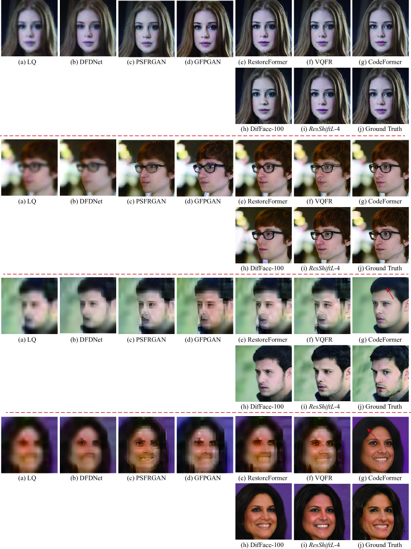
Figure 12: Qualitative results of different methods on the synthetic CelebA-Test dataset for blind face restoration. We annotate the diffusion-based methods with the format of “Method-A”, where “A” represents the number of sampling steps. Please zoom in for a better view.

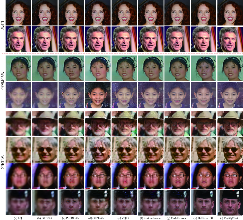
Figure 13: Qualitative results of different methods on three real-world datasets for blind face restoration. We annotate the diffusion-based methods with the format of “Method-A”, where “A” represents the number of sampling steps. Please zoom in for a better view.

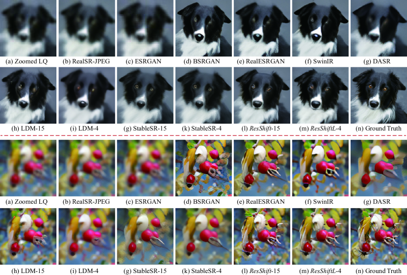
Figure 14: Qualitative results of different methods on the synthetic ImageNet-Test dataset for image super-resolution. Please zoom in for a better view.

References

- [1] S. Gu, Q. Xie, D. Meng, W. Zuo, X. Feng, and L. Zhang, “Weighted nuclear norm minimization and its applications to low level vision,” International Journal of Computer Vision (IJCV), vol. 121, pp. 183–208, 2017.
- [2] K. Zhang, W. Zuo, Y. Chen, D. Meng, and L. Zhang, “Beyond a gaussian denoiser: Residual learning of deep cnn for image denoising,” IEEE Transactions on Image Processing (TIP), vol. 26, no. 7, pp. 3142–3155, 2017.
- [3] W. Dong, L. Zhang, G. Shi, and X. Li, “Nonlocally centralized sparse representation for image restoration,” IEEE Transactions on Image Processing (TIP), vol. 22, no. 4, pp. 1620–1630, 2012.
- [4] C. Dong, C. C. Loy, K. He, and X. Tang, “Image super-resolution using deep convolutional networks,” IEEE Transactions on Pattern Analysis and Machine Intelligence (TPAMI), vol. 38, no. 2, pp. 295–307, 2015.
- [5] J. Yu, Z. Lin, J. Yang, X. Shen, X. Lu, and T. S. Huang, “Free-form image inpainting with gated convolution,” in Proceedings of the IEEE/CVF International Conference on Computer Vision (ICCV), 2019, pp. 4471–4480.
- [6] R. Suvorov, E. Logacheva, A. Mashikhin, A. Remizova, A. Ashukha, A. Silvestrov, N. Kong, H. Goka, K. Park, and V. Lempitsky, “Resolution-robust large mask inpainting with fourier convolutions,” in Proceedings of the IEEE/CVF Winter conference on Applications of Computer Vision (WACV), 2022, pp. 2149–2159.
- [7] J. Sohl-Dickstein, E. Weiss, N. Maheswaranathan, and S. Ganguli, “Deep unsupervised learning using nonequilibrium thermodynamics,” in International Conference on Machine Learning (ICML). PMLR, 2015, pp. 2256–2265.
- [8] J. Ho, A. Jain, and P. Abbeel, “Denoising diffusion probabilistic models,” in Proceedings of Advances in Neural Information Processing Systems (NeurIPS), vol. 33, 2020, pp. 6840–6851.
- [9] P. Dhariwal and A. Nichol, “Diffusion models beat gans on image synthesis,” in Proceedings of Advances in Neural Information Processing Systems (NeurIPS), vol. 34, 2021, pp. 8780–8794.
- [10] I. Goodfellow, J. Pouget-Abadie, M. Mirza, B. Xu, D. Warde-Farley, S. Ozair, A. Courville, and Y. Bengio, “Generative adversarial nets,” in Proceedings of Advances in Neural Information Processing Systems (NeurIPS), vol. 27, 2014.
- [11] A. Brock, J. Donahue, and K. Simonyan, “Large scale GAN training for high fidelity natural image synthesis,” in Proceedings of International Conference on Learning Representations (ICLR), 2019.
- [12] M. Delbracio and P. Milanfar, “Inversion by direct iteration: An alternative to denoising diffusion for image restoration,” Transactions on Machine Learning Research (TMLR), 2023.
- [13] Z. Luo, F. K. Gustafsson, Z. Zhao, J. Sjölund, and T. B. Schön, “Image restoration with mean-reverting stochastic differential equations,” in International Conference on Machine Learning (ICML), vol. 202. PMLR, 2023, pp. 23 045–23 066.
- [14] J. Whang, M. Delbracio, H. Talebi, C. Saharia, A. G. Dimakis, and P. Milanfar, “Deblurring via stochastic refinement,” in Proceedings of the IEEE/CVF Conference on Computer Vision and Pattern Recognition (CVPR), 2022, pp. 16 293–16 303.
- [15] N. Murata, K. Saito, C.-H. Lai, Y. Takida, T. Uesaka, Y. Mitsufuji, and S. Ermon, “GibbsDDRM: A partially collapsed Gibbs sampler for solving blind inverse problems with denoising diffusion restoration,” in International Conference on Machine Learning (ICML), vol. 202, 2023, pp. 25 501–25 522.
- [16] C. Meng, Y. He, Y. Song, J. Song, J. Wu, J.-Y. Zhu, and S. Ermon, “Sdedit: Guided image synthesis and editing with stochastic differential equations,” in Proceedings of International Conference on Learning Representations (ICLR), 2021.
- [17] A. Lugmayr, M. Danelljan, A. Romero, F. Yu, R. Timofte, and L. Van Gool, “Repaint: Inpainting using denoising diffusion probabilistic models,” in Proceedings of the IEEE/CVF Conference on Computer Vision and Pattern Recognition (CVPR), June 2022, pp. 11 461–11 471.
- [18] H. Chung, B. Sim, and J. C. Ye, “Come-closer-diffuse-faster: Accelerating conditional diffusion models for inverse problems through stochastic contraction,” in Proceedings of the IEEE/CVF Conference on Computer Vision and Pattern Recognition (CVPR), 2022, pp. 12 413–12 422.
- [19] Z. Yue and C. C. Loy, “Difface: Blind face restoration with diffused error contraction,” arXiv preprint arXiv:2212.06512, 2022.
- [20] Y. Song, J. Sohl-Dickstein, D. P. Kingma, A. Kumar, S. Ermon, and B. Poole, “Score-based generative modeling through stochastic differential equations,” in Proceedings of International Conference on Learning Representations (ICLR), 2021.
- [21] C. Saharia, W. Chan, H. Chang, C. Lee, J. Ho, T. Salimans, D. Fleet, and M. Norouzi, “Palette: Image-to-image diffusion models,” in Proceedings of ACM SIGGRAPH Conference, 2022, pp. 1–10.
- [22] Z. Liang, Z. Li, S. Zhou, C. Li, and C. C. Loy, “Control color: Multimodal diffusion-based interactive image colorization,” arXiv preprint arXiv:2402.10855, 2024.
- [23] C. Saharia, J. Ho, W. Chan, T. Salimans, D. J. Fleet, and M. Norouzi, “Image super-resolution via iterative refinement,” IEEE Transactions on Pattern Analysis and Machine Intelligence (TPAMI), 2022.
- [24] H. Chung, B. Sim, D. Ryu, and J. C. Ye, “Improving diffusion models for inverse problems using manifold constraints,” in Proceedings of Advances in Neural Information Processing Systems (NeurIPS), vol. 35, 2022, pp. 25 683–25 696.
- [25] R. Rombach, A. Blattmann, D. Lorenz, P. Esser, and B. Ommer, “High-resolution image synthesis with latent diffusion models,” in Proceedings of the IEEE/CVF Conference on Computer Vision and Pattern Recognition (CVPR), 2022, pp. 10 684–10 695.
- [26] H. Li, Y. Yang, M. Chang, S. Chen, H. Feng, Z. Xu, Q. Li, and Y. Chen, “Srdiff: Single image super-resolution with diffusion probabilistic models,” Neurocomputing, vol. 479, pp. 47–59, 2022.
- [27] B. Xia, Y. Zhang, S. Wang, Y. Wang, X. Wu, Y. Tian, W. Yang, and L. Van Gool, “Diffir: Efficient diffusion model for image restoration,” in Proceedings of the IEEE/CVF International Conference on Computer Vision (ICCV), 2023, pp. 13 095–13 105.
- [28] B. Kawar, M. Elad, S. Ermon, and J. Song, “Denoising diffusion restoration models,” in Proceedings of Advances in Neural Information Processing Systems (NeurIPS), 2022.
- [29] J. Wang, Z. Yue, S. Zhou, K. C. Chan, and C. C. Loy, “Exploiting diffusion prior for real-world image super-resolution,” arXiv preprint arXiv:2305.07015, 2023.
- [30] T. Yang, P. Ren, X. Xie, and L. Zhang, “Pixel-aware stable diffusion for realistic image super-resolution and personalized stylization,” arXiv preprint arXiv:2308.14469, 2023.
- [31] H. Sun, W. Li, J. Liu, H. Chen, R. Pei, X. Zou, Y. Yan, and Y. Yang, “CoSeR: Bridging image and language for cognitive super-resolution,” arXiv preprint arXiv:2311.16512, 2023.
- [32] Y. Wang, J. Yu, and J. Zhang, “Zero-shot image restoration using denoising diffusion null-space model,” in Proceedings of International Conference on Learning Representations (ICLR), 2023.
- [33] Y. Zhu, K. Zhang, J. Liang, J. Cao, B. Wen, R. Timofte, and L. Van Gool, “Denoising diffusion models for plug-and-play image restoration,” in Proceedings of the IEEE/CVF International Conference on Computer Vision Workshops (CVPR-W), 2023, pp. 1219–1229.
- [34] R. Wu, T. Yang, L. Sun, Z. Zhang, S. Li, and L. Zhang, “SeeSR: Towards semantics-aware real-world image super-resolution,” arXiv preprint arXiv:2311.16518, 2023.
- [35] A. Q. Nichol and P. Dhariwal, “Improved denoising diffusion probabilistic models,” in International Conference on Machine Learning (ICML). PMLR, 2021, pp. 8162–8171.
- [36] J. Song, C. Meng, and S. Ermon, “Denoising diffusion implicit models,” in Proceedings of International Conference on Learning Representations (ICLR), 2021.
- [37] C. Lu, Y. Zhou, F. Bao, J. Chen, C. Li, and J. Zhu, “DPM-solver: A fast ODE solver for diffusion probabilistic model sampling in around 10 steps,” in Proceedings of Advances in Neural Information Processing Systems (NeurIPS), 2022.
- [38] X. Wang, L. Xie, C. Dong, and Y. Shan, “Real-esrgan: Training real-world blind super-resolution with pure synthetic data,” in Proceedings of the IEEE/CVF International Conference on Computer Vision Workshops (ICCV-W), 2021, pp. 1905–1914.
- [39] K. Zhang, J. Liang, L. Van Gool, and R. Timofte, “Designing a practical degradation model for deep blind image super-resolution,” in Proceedings of the IEEE/CVF International Conference on Computer Vision (ICCV), 2021, pp. 4791–4800.
- [40] J. Liang, J. Cao, G. Sun, K. Zhang, L. Van Gool, and R. Timofte, “Swinir: Image restoration using swin transformer,” in Proceedings of the IEEE/CVF International Conference on Computer Vision Workshops (ICCV-W), 2021, pp. 1833–1844.
- [41] Z. Yue, J. Wang, and C. C. Loy, “Resshift: Efficient diffusion model for image super-resolution by residual shifting,” in Proceedings of Advances in Neural Information Processing Systems (NeurIPS), 2023.
- [42] A. Foi, M. Trimeche, V. Katkovnik, and K. Egiazarian, “Practical poissonian-gaussian noise modeling and fitting for single-image raw-data,” IEEE Transactions on Image Processing (TIP), vol. 17, no. 10, pp. 1737–1754, 2008.
- [43] D. Meng and F. De La Torre, “Robust matrix factorization with unknown noise,” in Proceedings of the IEEE/CVF International Conference on Computer Vision (ICCV), 2013, pp. 1337–1344.
- [44] X. Cao, Q. Zhao, D. Meng, Y. Chen, and Z. Xu, “Robust low-rank matrix factorization under general mixture noise distributions,” IEEE Transactions on Image Processing (TIP), vol. 25, no. 10, pp. 4677–4690, 2016.
- [45] F. Zhu, G. Chen, J. Hao, and P.-A. Heng, “Blind image denoising via dependent dirichlet process tree,” IEEE Transactions on Pattern Analysis and Machine Intelligence (TPAMI), vol. 39, no. 8, pp. 1518–1531, 2016.
- [46] Z. Yue, D. Meng, Y. Sun, and Q. Zhao, “Hyperspectral image restoration under complex multi-band noises,” Remote Sensing, vol. 10, no. 10, p. 1631, 2018.
- [47] L. I. Rudin, S. Osher, and E. Fatemi, “Nonlinear total variation based noise removal algorithms,” Physica D: Nonlinear Phenomena, vol. 60, no. 1-4, pp. 259–268, 1992.
- [48] E. P. Simoncelli and E. H. Adelson, “Noise removal via bayesian wavelet coring,” in Proceedings of IEEE International Conference on Image Processing (ICIP), vol. 1, 1996, pp. 379–382.
- [49] A. Buades, B. Coll, and J.-M. Morel, “A non-local algorithm for image denoising,” in Proceedings of the IEEE/CVF Conference on Computer Vision and Pattern Recognition (CVPR), vol. 2, 2005, pp. 60–65.
- [50] W. Dong, L. Zhang, G. Shi, and X. Wu, “Image deblurring and super-resolution by adaptive sparse domain selection and adaptive regularization,” IEEE Transactions on Image Processing (TIP), vol. 20, no. 7, pp. 1838–1857, 2011.
- [51] S. Gu, W. Zuo, Q. Xie, D. Meng, X. Feng, and L. Zhang, “Convolutional sparse coding for image super-resolution,” in Proceedings of the IEEE/CVF International Conference on Computer Vision (ICCV), 2015, pp. 1823–1831.
- [52] J. Xu, L. Zhang, D. Zhang, and X. Feng, “Multi-channel weighted nuclear norm minimization for real color image denoising,” in Proceedings of the IEEE/CVF International Conference on Computer Vision (ICCV), 2017.
- [53] K. He, J. Sun, and X. Tang, “Single image haze removal using dark channel prior,” IEEE Transactions on Pattern Analysis and Machine Intelligence (TPAMI), vol. 33, no. 12, pp. 2341–2353, 2010.
- [54] J. Pan, D. Sun, H. Pfister, and M.-H. Yang, “Blind image deblurring using dark channel prior,” in Proceedings of the IEEE/CVF Conference on Computer Vision and Pattern Recognition (CVPR), 2016, pp. 1628–1636.
- [55] J. Sun, W. Cao, Z. Xu, and J. Ponce, “Learning a convolutional neural network for non-uniform motion blur removal,” in Proceedings of the IEEE/CVF Conference on Computer Vision and Pattern Recognition (CVPR), June 2015.
- [56] W. Shi, J. Caballero, F. Huszár, J. Totz, A. P. Aitken, R. Bishop, D. Rueckert, and Z. Wang, “Real-time single image and video super-resolution using an efficient sub-pixel convolutional neural network,” in Proceedings of the IEEE/CVF Conference on Computer Vision and Pattern Recognition (CVPR), 2016, pp. 1874–1883.
- [57] Y. Tai, J. Yang, X. Liu, and C. Xu, “Memnet: A persistent memory network for image restoration,” in Proceedings of the IEEE/CVF International Conference on Computer Vision (ICCV), 2017, pp. 4539–4547.
- [58] W.-S. Lai, J.-B. Huang, N. Ahuja, and M.-H. Yang, “Deep laplacian pyramid networks for fast and accurate super-resolution,” in Proceedings of the IEEE/CVF Conference on Computer Vision and Pattern Recognition (CVPR), 2017, pp. 624–632.
- [59] M. Haris, G. Shakhnarovich, and N. Ukita, “Deep back-projection networks for super-resolution,” in Proceedings of the IEEE/CVF Conference on Computer Vision and Pattern Recognition (CVPR), 2018, pp. 1664–1673.
- [60] Y. Zhang, Y. Tian, Y. Kong, B. Zhong, and Y. Fu, “Residual dense network for image super-resolution,” in Proceedings of the IEEE/CVF Conference on Computer Vision and Pattern Recognition (CVPR), 2018, pp. 2472–2481.
- [61] X. Hu, H. Mu, X. Zhang, Z. Wang, T. Tan, and J. Sun, “Meta-sr: A magnification-arbitrary network for super-resolution,” in Proceedings of the IEEE/CVF Conference on Computer Vision and Pattern Recognition (CVPR), 2019, pp. 1575–1584.
- [62] Z. Wan, J. Zhang, D. Chen, and J. Liao, “High-fidelity pluralistic image completion with transformers,” in Proceedings of the IEEE/CVF International Conference on Computer Vision (ICCV), 2021, pp. 4692–4701.
- [63] S. W. Zamir, A. Arora, S. Khan, M. Hayat, F. S. Khan, and M.-H. Yang, “Restormer: Efficient transformer for high-resolution image restoration,” in Proceedings of the IEEE/CVF Conference on Computer Vision and Pattern Recognition (CVPR), 2022, pp. 5728–5739.
- [64] Z. Wang, X. Cun, J. Bao, W. Zhou, J. Liu, and H. Li, “Uformer: A general u-shaped transformer for image restoration,” in Proceedings of the IEEE/CVF Conference on Computer Vision and Pattern Recognition (CVPR), 2022, pp. 17 683–17 693.
- [65] K. Zhang, W. Zuo, and L. Zhang, “Learning a single convolutional super-resolution network for multiple degradations,” in Proceedings of the IEEE/CVF Conference on Computer Vision and Pattern Recognition (CVPR), 2018, pp. 3262–3271.
- [66] D. Simon and M. Elad, “Rethinking the csc model for natural images,” in Proceedings of Advances in Neural Information Processing Systems (NeurIPS), 2019.
- [67] K. Zhang, L. V. Gool, and R. Timofte, “Deep unfolding network for image super-resolution,” in Proceedings of the IEEE/CVF Conference on Computer Vision and Pattern Recognition (CVPR), 2020, pp. 3217–3226.
- [68] D. Liu, B. Wen, Y. Fan, C. C. Loy, and T. S. Huang, “Non-local recurrent network for image restoration,” Proceedings of Advances in Neural Information Processing Systems (NeurIPS), vol. 31, 2018.
- [69] D. Ulyanov, A. Vedaldi, and V. Lempitsky, “Deep image prior,” in Proceedings of the IEEE/CVF Conference on Computer Vision and Pattern Recognition (CVPR), 2018, pp. 9446–9454.
- [70] J. Gu, Y. Shen, and B. Zhou, “Image processing using multi-code gan prior,” in Proceedings of the IEEE/CVF Conference on Computer Vision and Pattern Recognition (CVPR), 2020.
- [71] X. Pan, X. Zhan, B. Dai, D. Lin, C. C. Loy, and P. Luo, “Exploiting deep generative prior for versatile image restoration and manipulation,” IEEE Transactions on Pattern Analysis and Machine Intelligence (TPAMI), vol. 44, no. 11, pp. 7474–7489, 2022.
- [72] X. Wang, K. Yu, S. Wu, J. Gu, Y. Liu, C. Dong, Y. Qiao, and C. Change Loy, “ESRGAN: Enhanced super-resolution generative adversarial networks,” in Proceedings of the European Conference on Computer Vision Workshops (ECCV-W), 2018.
- [73] Z. Yue, Q. Zhao, J. Xie, L. Zhang, D. Meng, and K.-Y. K. Wong, “Blind image super-resolution with elaborate degradation modeling on noise and kernel,” in Proceedings of the IEEE/CVF Conference on Computer Vision and Pattern Recognition (CVPR), 2022, pp. 2128–2138.
- [74] A. Lugmayr, M. Danelljan, L. Van Gool, and R. Timofte, “SRFlow: Learning the super-resolution space with normalizing flow,” in Proceedings of the European Conference on Computer Vision (ECCV), 2020, pp. 715–732.
- [75] L. Zhang, A. Rao, and M. Agrawala, “Adding conditional control to text-to-image diffusion models,” in Proceedings of the IEEE/CVF International Conference on Computer Vision (ICCV), 2023, pp. 3836–3847.
- [76] P. Esser, R. Rombach, and B. Ommer, “Taming transformers for high-resolution image synthesis,” in Proceedings of the IEEE/CVF Conference on Computer Vision and Pattern Recognition (CVPR), 2021, pp. 12 873–12 883.
- [77] R. Zhang, P. Isola, A. A. Efros, E. Shechtman, and O. Wang, “The unreasonable effectiveness of deep features as a perceptual metric,” in Proceedings of the IEEE/CVF Conference on Computer Vision and Pattern Recognition (CVPR), 2018, pp. 586–595.
- [78] Y. Song and S. Ermon, “Generative modeling by estimating gradients of the data distribution,” in Proceedings of Advances in Neural Information Processing Systems (NeurIPS), vol. 32, 2019.
- [79] A. Vaswani, N. Shazeer, N. Parmar, J. Uszkoreit, L. Jones, A. N. Gomez, Ł. Kaiser, and I. Polosukhin, “Attention is all you need,” in Proceedings of Advances in Neural Information Processing Systems (NeurIPS), 2017.
- [80] Z. Liu, Y. Lin, Y. Cao, H. Hu, Y. Wei, Z. Zhang, S. Lin, and B. Guo, “Swin transformer: Hierarchical vision transformer using shifted windows,” in Proceedings of the IEEE/CVF International Conference on Computer Vision (ICCV), 2021, pp. 10 012–10 022.
- [81] J. Deng, W. Dong, R. Socher, L.-J. Li, K. Li, and L. Fei-Fei, “Imagenet: A large-scale hierarchical image database,” in Proceedings of the IEEE/CVF Conference on Computer Vision and Pattern Recognition (CVPR), 2009, pp. 248–255.
- [82] D. P. Kingma and J. Ba, “Adam: A method for stochastic optimization.” in Proceedings of International Conference on Learning Representations (ICLR), 2015.
- [83] A. Paszke, S. Gross, F. Massa, A. Lerer, J. Bradbury, G. Chanan, T. Killeen, Z. Lin, N. Gimelshein, L. Antiga et al., “Pytorch: An imperative style, high-performance deep learning library,” in Proceedings of Advances in Neural Information Processing Systems (NeurIPS), vol. 32, 2019.
- [84] I. Loshchilov and F. Hutter, “SGDR: Stochastic gradient descent with warm restarts,” in Proceedings of International Conference on Learning Representations (ICLR), 2017.
- [85] M. Bevilacqua, A. Roumy, C. Guillemot, and M. L. Alberi-Morel, “Low-complexity single-image super-resolution based on nonnegative neighbor embedding,” 2012.
- [86] R. Zeyde, M. Elad, and M. Protter, “On single image scale-up using sparse-representations,” in International Conference on Curves and Surfaces. Springer, 2012, pp. 711–730.
- [87] J.-B. Huang, A. Singh, and N. Ahuja, “Single image super-resolution from transformed self-exemplars,” in Proceedings of the IEEE/CVF Conference on Computer Vision and Pattern Recognition (CVPR), 2015, pp. 5197–5206.
- [88] J. Cai, H. Zeng, H. Yong, Z. Cao, and L. Zhang, “Toward real-world single image super-resolution: A new benchmark and a new model,” in Proceedings of the IEEE/CVF International Conference on Computer Vision (ICCV), 2019, pp. 3086–3095.
- [89] D. Martin, C. Fowlkes, D. Tal, and J. Malik, “A database of human segmented natural images and its application to evaluating segmentation algorithms and measuring ecological statistics,” in Proceedings of the IEEE/CVF International Conference on Computer Vision (ICCV), vol. 2, 2001, pp. 416–423.
- [90] Y. Matsui, K. Ito, Y. Aramaki, A. Fujimoto, T. Ogawa, T. Yamasaki, and K. Aizawa, “Sketch-based manga retrieval using manga109 dataset,” Multimedia Tools and Applications, vol. 76, pp. 21 811–21 838, 2017.
- [91] A. Ignatov, N. Kobyshev, R. Timofte, K. Vanhoey, and L. Van Gool, “Dslr-quality photos on mobile devices with deep convolutional networks,” in Proceedings of the IEEE/CVF International Conference on Computer Vision (ICCV), 2017.
- [92] K. Zhang, W. Zuo, and L. Zhang, “Ffdnet: Toward a fast and flexible solution for cnn-based image denoising,” IEEE Transactions on Image Processing (TIP), vol. 27, no. 9, pp. 4608–4622, 2018.
- [93] X. Lin, J. He, Z. Chen, Z. Lyu, B. Fei, B. Dai, W. Ouyang, Y. Qiao, and C. Dong, “Diffbir: Towards blind image restoration with generative diffusion prior,” arXiv preprint arXiv:2308.15070, 2023.
- [94] X. Ji, Y. Cao, Y. Tai, C. Wang, J. Li, and F. Huang, “Real-world super-resolution via kernel estimation and noise injection,” in Proceedings of the IEEE/CVF International Conference on Computer Vision Workshops (CVPR-W), 2020, pp. 466–467.
- [95] J. Liang, H. Zeng, and L. Zhang, “Efficient and degradation-adaptive network for real-world image super-resolution,” in Proceedings of the European Conference on Computer Vision (ECCV), 2022, pp. 574–591.
- [96] Z. Wang, A. Bovik, H. Sheikh, and E. Simoncelli, “Image quality assessment: from error visibility to structural similarity,” IEEE Transactions on Image Processing (TIP), vol. 13, no. 4, pp. 600–612, 2004.
- [97] J. Wang, K. C. Chan, and C. C. Loy, “Exploring clip for assessing the look and feel of images,” in Proceedings of the AAAI Conference on Artificial Intelligence, 2023.
- [98] J. Ke, Q. Wang, Y. Wang, P. Milanfar, and F. Yang, “Musiq: Multi-scale image quality transformer,” in Proceedings of the IEEE/CVF International Conference on Computer Vision (ICCV), 2021, pp. 5148–5157.
- [99] A. Radford, J. W. Kim, C. Hallacy, A. Ramesh, G. Goh, S. Agarwal, G. Sastry, A. Askell, P. Mishkin, J. Clark et al., “Learning transferable visual models from natural language supervision,” in International Conference on Machine Learning (ICML), 2021, pp. 8748–8763.
- [100] C. Schuhmann, R. Vencu, R. Beaumont, R. Kaczmarczyk, C. Mullis, A. Katta, T. Coombes, J. Jitsev, and A. Komatsuzaki, “Laion-400m: Open dataset of clip-filtered 400 million image-text pairs,” in Proceedings of Advances in Neural Information Processing Systems Workshops (NeurIPS-W), 2021.
- [101] Y. Blau and T. Michaeli, “The perception-distortion tradeoff,” in Proceedings of the IEEE/CVF Conference on Computer Vision and Pattern Recognition (CVPR), June 2018.
- [102] T. Karras, S. Laine, and T. Aila, “A style-based generator architecture for generative adversarial networks,” in Proceedings of the IEEE/CVF Conference on Computer Vision and Pattern Recognition (CVPR), 2019, pp. 4401–4410.
- [103] T. Karras, T. Aila, S. Laine, and J. Lehtinen, “Progressive growing of GANs for improved quality, stability, and variation,” in Proceedings of International Conference on Learning Representations (ICLR), 2018.
- [104] X. Wang, Y. Li, H. Zhang, and Y. Shan, “Towards real-world blind face restoration with generative facial prior,” in Proceedings of the IEEE/CVF Conference on Computer Vision and Pattern Recognition (CVPR), 2021, pp. 9168–9178.
- [105] S. Zhou, K. Chan, C. Li, and C. C. Loy, “Towards robust blind face restoration with codebook lookup transformer,” in Proceedings of Advances in Neural Information Processing Systems (NeurIPS), 2022.
- [106] G. B. Huang, M. Mattar, T. Berg, and E. Learned-Miller, “Labeled faces in the wild: A database forstudying face recognition in unconstrained environments,” in Workshop on faces in ’Real-Life’ Images: detection, alignment, and recognition, 2008.
- [107] S. Yang, P. Luo, C.-C. Loy, and X. Tang, “Wider face: A face detection benchmark,” in Proceedings of the IEEE/CVF Conference on Computer Vision and Pattern Recognition (CVPR), 2016, pp. 5525–5533.
- [108] X. Li, C. Chen, S. Zhou, X. Lin, W. Zuo, and L. Zhang, “Blind face restoration via deep multi-scale component dictionaries,” in Proceedings of the European Conference on Computer Vision (ECCV), 2020.
- [109] C. Chen, X. Li, L. Yang, X. Lin, L. Zhang, and K.-Y. K. Wong, “Progressive semantic-aware style transformation for blind face restoration,” in Proceedings of the IEEE/CVF Conference on Computer Vision and Pattern Recognition (CVPR), 2021.
- [110] Z. Wang, J. Zhang, R. Chen, W. Wang, and P. Luo, “Restoreformer: High-quality blind face restoration from undegraded key-value pairs,” in Proceedings of the IEEE/CVF Conference on Computer Vision and Pattern Recognition (CVPR), 2022.
- [111] Y. Gu, X. Wang, L. Xie, C. Dong, G. Li, Y. Shan, and M.-M. Cheng, “Vqfr: Blind face restoration with vector-quantized dictionary and parallel decoder,” in Proceedings of the European Conference on Computer Vision (ECCV), 2022, pp. 126–143.
- [112] Z. Wang, A. C. Bovik, H. R. Sheikh, and E. P. Simoncelli, “Image quality assessment: from error visibility to structural similarity,” IEEE Transactions on Image Processing (TIP), vol. 13, no. 4, pp. 600–612, 2004.
- [113] M. Heusel, H. Ramsauer, T. Unterthiner, B. Nessler, and S. Hochreiter, “Gans trained by a two time-scale update rule converge to a local nash equilibrium,” in Proceedings of Advances in Neural Information Processing Systems (NeurIPS), 2017.
- [114] J. Deng, J. Guo, N. Xue, and S. Zafeiriou, “Arcface: Additive angular margin loss for deep face recognition,” in Proceedings of the IEEE/CVF Conference on Computer Vision and Pattern Recognition (CVPR), 2019.