How does promoting the minority fraction affect generalization? A theoretical study of the one-hidden-layer neural network on group imbalance

Abstract

Group imbalance has been a known problem in empirical risk minimization (ERM), where the achieved high average accuracy is accompanied by low accuracy in a minority group. Despite algorithmic efforts to improve the minority group accuracy, a theoretical generalization analysis of ERM on individual groups remains elusive. By formulating the group imbalance problem with the Gaussian Mixture Model, this paper quantifies the impact of individual groups on the sample complexity, the convergence rate, and the average and group-level testing performance. Although our theoretical framework is centered on binary classification using a one-hidden-layer neural network, to the best of our knowledge, we provide the first theoretical analysis of the group-level generalization of ERM in addition to the commonly studied average generalization performance. Sample insights of our theoretical results include that when all group-level co-variance is in the medium regime and all mean are close to zero, the learning performance is most desirable in the sense of a small sample complexity, a fast training rate, and a high average and group-level testing accuracy. Moreover, we show that increasing the fraction of the minority group in the training data does not necessarily improve the generalization performance of the minority group. Our theoretical results are validated on both synthetic and empirical datasets, such as CelebA and CIFAR-10 in image classification.

I Introduction

Training neural networks with empirical risk minimization (ERM) is a common practice to reduce the average loss of a machine learning task evaluated on a dataset. However, recent findings [1, 2, 3, 4, 5] have shown empirical evidence about a critical challenge of ERM, known as group imbalance, where a well-trained model that has high average accuracy may have significant errors on the minority group that infrequently appears in the data. Moreover, the group attributes that determine the majority and minority groups are usually hidden and unknown during the training. The training set can be augmented by data augmentation methods [6] with varying performance, such as cropping and rotation [7], noise injection [8], and generative adversarial network (GAN)-based methods [9].

As ERM is a prominent method and enjoys great empirical success, it is important to characterize the impact of ERM on group imbalance theoretically. However, the technical difficulty of analyzing the nonconvex ERM problem of neural networks results from the concatenation of nonlinear functions across layers, and the existing generalization analyses of ERM often require strong assumptions and focus on the average performance of all data. For example, the neural tangent kernel type of analysis [10, 11, 12, 13, 14, 15, 16, 17] linearizes the neural network around the random initialization. The generalization results are independent of the feature distribution and cannot be exploited to characterize the impact of individual groups. Ref. [14] provides the sample complexity analysis when the data comes from the mixtures of well-separated distributions but still cannot characterize the learning performance of individual groups. In another line of works [18, 19, 20, 21, 22, 23, 24, 25, 26, 27, 28], people make data assumptions that the labels are determined merely by some input features and are irrelevant to other features or model parameters. The generalization analysis characterizes how the neurons learn important features. Our work follows the line of works [29, 30, 31, 32, 33, 34], where the label of each data is generated by both the input distribution and the ground-truth model so that group imbalance can be characterized.

Contribution: To the best of our knowledge, this paper provides the first theoretical characterization of both the average and group-level generalization of a one-hidden-layer neural network trained by ERM on data generated from a mixture of distributions. This paper considers the binary classification problem with the cross entropy loss function, with training data generated by a ground-truth neural network with known architecture and unknown weights. The optimization problem is challenging due to a high non-convexity from the multi-neuron architecture and the non-linear sigmoid activation.

Assuming the features follow a Gaussian Mixture Model (GMM), where samples of each group are generated from a Gaussian distribution with an arbitrary mean vector and co-variance matrix, this paper quantifies the impact of individual groups on the sample complexity, the training convergence rate, and the average and group-level test error. The training algorithm is the gradient descent following a tensor initialization and converges linearly. Our key results include

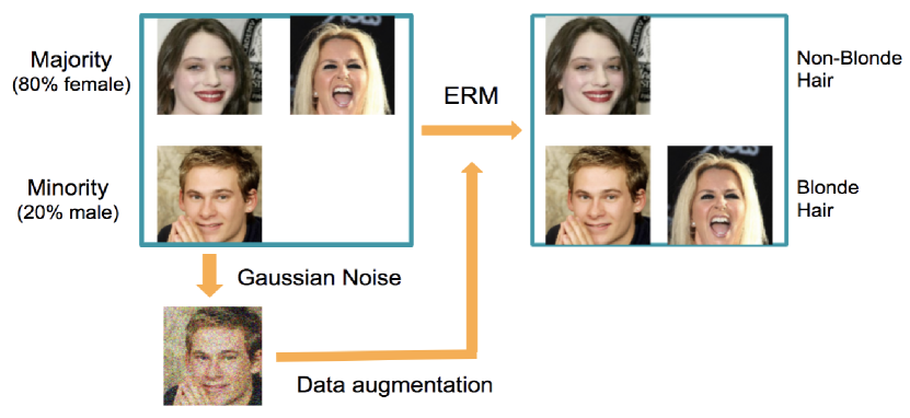
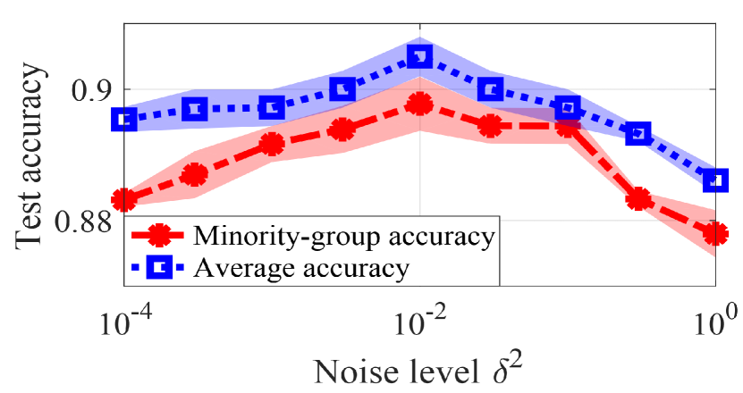
Figure 1: Group imbalance experiment. (a) Binary classification on CelebA dataset using Gaussian augmentation to control the minority group co-variance. (b) Test accuracy against the augmented noise level.

(1) Medium-range group-level co-variance enhances the learning performance. When a group-level co-variance deviates from the medium regime, the learning performance degrades in terms of higher sample complexity, slower convergence in training, and worse average and group-level generalization performance. As shown in Figure 1(a), we introduce Gaussian augmentation to control the co-variance level of the minority group in the CelebA dataset [35]. The learned model achieves the highest test accuracy when the co-variance is at the medium level, see Figure 1(b). Another implication is that the diverse performance of different data augmentation methods might partially result from the different group-level co-variance introduced by these methods. Furthermore, although our setup does not directly model the batch normalization approach [36] that modifies the mean and variance in each layer to achieve fast and stable convergence, our result provides a theoretical insight that co-variance indeed affects the learning performance.

(2) Group-level mean shifts from zero hurt the learning performance. When a group-level mean deviates from zero, the sample complexity increases, the algorithm converges slower, and both the average and group-level test error increases. Thus, the learning performance is improved if each distribution is zero-mean. This paper provides a similar theoretical insight to practical tricks such as whitening [37], subgroup shift [38, 39], population shift [40, 41] and the pre-processing of making data zero-mean [42], that data mean affects the learning performance.

(3) Increasing the fraction of the minority group in the training data does not always improve its generalization performance. The generalization performance is also affected by the mean and co-variance of individual groups. In fact, increasing the fraction of the minority group in the training data can have a completely opposite impact in different datasets.

II Background and Related Work

Improving the minority-group performance with known group attributes. With known group attributes, distributionally robust optimization (DRO) [4] minimizes the worst-group training loss instead of solving ERM. DRO is more computationally expensive than ERM and does not always outperform ERM in the minority-group test error. Spurious correlations [3] can be viewed as one reason of group imbalance, where strong associations between labels and irrelevant features exist in training samples. Different from the approaches that address spurious correlations, such as down-sampling the majority [43, 44], up-weight the minority group [45], and removing spurious features [46, 47], this paper does not require the special model of spurious correlations and any group attribute information.

Imbalance learning and long-tailed learning focus on learning from imbalanced data with a long-tailed distribution, which means that a few classes of the data make up the majority of the dataset, while the majority of classes have little data samples [48, 49, 50, 51, 52, 53, 54, 55, 56]. Some works [49, 56] claimed that naively increasing the number of the minority does not always improve the generalization. Therefore, some recent works develop novel oversampling and data augmentation methods [53, 52, 55] that can promote the minority fraction by generating diverse and context-rich minority data. However, there are very limited theoretical explanations of how these techniques affect the generalization.

Generalization performance with the standard Gaussian input for one-hidden-layer neural networks. [57, 58, 59, 60] consider infinite training samples. [29] characterize the sample complexity of fully connected neural networks with smooth activation functions. [61, 62, 34] extend to the non-smooth ReLU activation for fully-connected and convolutional neural networks, respectively. [31] analyzes the cross entropy loss function for binary classification problems. [30] analyzes the generalizability of graph neural networks for both regression and binary classification problems. One-hidden-layer case of neural network pruning and self-training are also studied in [63] and [32], respectively.

Theoretical characterization of learning performance from other input distributions for one-hidden-layer neural networks. [64] analyzes the training loss with a single Gaussian with an arbitrary co-variance. [65] quantifies the SGD evolution trained on the Gaussian mixture model. When the hidden layer only contains one neuron, [66] analyzes rotationally invariant distributions. With an infinite number of neurons and an infinite input dimension, [67] analyzes the generalization error based on the mean-field analysis for distributions like Gaussian Mixture with the same mean. [68] considers inputs with low-dimensional structures. No sample complexity is provided in all these works.

Notations:${\bm{Z}}$ is a matrix with $Z_{i,j}$ as the $(i,j)$-th entry. ${\bm{z}}$ is a vector with $z_{i}$ as the $i$-th entry. $[K]$ denotes the set including integers from $1$ to $K$. ${\bm{I}}_{d}$ and ${\bm{e}}_{i}$ represent the identity matrix in $\mathbb{R}^{d\times d}$ and the $i$-th standard basis vector, respectively. $\delta_{i}({\bm{Z}})$ denotes the $i$-th largest singular value of ${\bm{Z}}$. The matrix norm $\|{\bm{Z}}\|=\delta_{1}({\bm{Z}})$. $f(x)=O(g(x))$ (or $\Omega(g(x))$, $\Theta(g(x)))$ means that $f(x)$ increases at most, at least, or in the order of $g(x)$, respectively.

III Problem Formulation and Algorithm

We consider the classification problem with an unbalanced dataset using fully connected neural networks over $n$ independent training examples $\{({\bm{x}}_{i},y_{i})\}_{i=1}^{N}$ from a data distribution. The learning algorithm is to minimize the empirical risk function via gradient descent (GD). In what follows, we will present the data model and neural network model considered in this paper.

Data Model. Let ${\bm{x}}\in\mathbb{R}^{d}$ and $y\in\mathbb{R}$ denote the input feature and label, respectively. We consider an unbalanced dataset that consists of $L$ ($L\geq 2$) groups of data, where the feature ${\bm{x}}$ in the group $l$ ($l\in[L]$) is drawn from a multi-variate Gaussian distribution with mean ${\bm{\mu}}_{l}\in\mathbb{R}^{d}$, and covariance ${\bm{\Sigma}}_{l}\in\mathbb{R}^{d\times d}$. Specifically, ${\bm{x}}$ follows the Gaussian mixture model (GMM) [69, 70, 71, 72], denoted as ${\bm{x}}\sim\sum_{l=1}^{L}\lambda_{l}\mathcal{N}({\bm{\mu}}_{l},{\bm{\Sigma}}_{l})$. $\lambda_{l}\in(0,1)$ is the probability of sampling from distribution-$l$ and represents the expected fraction of group-$l$ data. $\sum_{l=1}^{L}\lambda_{l}=1$. Group $l$ is defined as a minority group if $\lambda_{l}$ is less than $1/L$. We use $\Psi=\{\lambda_{l},{\bm{\mu}}_{l},{\bm{\Sigma}}_{l},\forall l\}$ to denote all parameters of the mixture model. We consider binary classification with label $y$ generated by a ground-truth neural network with unknown weights ${\bm{W}}^{*}=[{\bm{w}}^{*}_{1},...,{\bm{w}}^{*}_{K}]\in\mathbb{R}^{d\times K}$ and sigmoid activation. function $\phi(x)=\frac{1}{1+\exp(-x)}$, where

$$\mathbb{P}(y=1|{\bm{x}})=H({\bm{W}}^{*},{\bm{x}}):=\frac{1}{K}\sum_{j=1}^{K}\phi({{\bm{w}}_{j}^{*}}^{\top}{\bm{x}}).$$ (1)

Learning model. Learning is performed over a neural network that has the same architecture as in (1), which is a one-hidden-layer fully connected neural network with its weights denoted by ${\bm{W}}\in\mathbb{R}^{d\times K}$. Given $n$ training samples $\{{\bm{x}}_{i},y_{i}\}_{i=1}^{n}$ where ${\bm{x}}_{i}$ follows the GMM model, and $y_{i}$ is from (1), we aim to find the model weights via solving the empirical risk minimization (ERM), where $f_{n}({\bm{W}})$ is the empirical risk,

$$\min_{{\bm{W}}\in\mathbb{R}^{d\times K}}f_{n}({\bm{W}}):=\frac{1}{n}\sum_{i=1}^{n}\ell({\bm{W}};{\bm{x}}_{i},y_{i}),$$ (2)

where $\ell({\bm{W}};{\bm{x}}_{i},y_{i})$ is the cross-entropy loss function, i.e.,

$$\ell({\bm{W}};{\bm{x}}_{i},y_{i})= -y_{i}\cdot\log(H({\bm{W}},{\bm{x}}_{i}))$$ (3)

$$-(1-y_{i})\cdot\log(1-H({\bm{W}},{\bm{x}}_{i})).$$

Note that for any permutation matrix ${\bm{P}}$, ${\bm{W}}{\bm{P}}$ corresponds permuting neurons of a network with weights ${\bm{W}}$. Therefore, $H({\bm{W}},{\bm{x}})=H({\bm{W}}{\bm{P}},{\bm{x}})$, and $f_{n}({\bm{W}}{\bm{P}})=f_{n}({\bm{W}})$. The estimation is considered successful if one finds any column permutation of ${\bm{W}}^{*}$.

The average generalization performance of a learned model ${\bm{W}}$ is evaluated by the average risk

$$\bar{f}({\bm{W}})=\mathbb{E}_{{\bm{x}}\sim\sum_{l=1}^{L}\lambda_{l}\mathcal{N}({\bm{\mu}}_{l},{\bm{\Sigma}}_{l})}\ell({\bm{W}};{\bm{x}}_{i},y_{i}),$$ (4)

and the generalization performance on group $l$ is evaluated by the group-$l$ risk

$$\bar{f}_{l}({\bm{W}})=\mathbb{E}_{{\bm{x}}\sim\mathcal{N}({\bm{\mu}}_{l},{\bm{\Sigma}}_{l})}\ell({\bm{W}};{\bm{x}}_{i},y_{i}).$$ (5)

Training Algorithm. Our algorithm starts from an initialization ${\bm{W}}_{0}\in\mathbb{R}^{d\times K}$ computed based on the tensor initialization method (Subroutine 1 in in Appendix) and then updates the iterates ${\bm{W}}_{t}$ using gradient descent with the step size $\eta_{0}$. The computational complexity of tensor initialization is $O(Knd)$. The per-iteration complexity of the gradient step is $O(Knd)$. We defer the details of Algorithm 1 in Supplementary Material.

1:Input: Training data $\{({\bm{x}}_{i},y_{i})\}_{i=1}^{n}$, the step size $\eta_{0}=O\Big{(}\big{(}\sum_{l=1}^{L}\lambda_{l}(\|\tilde{{\bm{\mu}}}_{l}\|_{\infty}+\|{\bm{\Sigma}}_{l}^{\frac{1}{2}}\|)^{2}\big{)}^{-1}\Big{)}$, the total number of iterations $T$

2:Initialization: ${\bm{W}}_{0}\leftarrow$ Tensor initialization method via Subroutine 1

3:Gradient Descent: for $t=0,1,\cdots,T-1$

$${\bm{W}}_{t+1} ={\bm{W}}_{t}-\eta_{0}\cdot\frac{1}{n}\sum_{i=1}^{n}(\nabla l({\bm{W}},{\bm{x}}_{i},y_{i})+\nu_{i})$$ (6)

$$={\bm{W}}_{t}-\eta_{0}\Big{(}\nabla f_{n}({\bm{W}})+\frac{1}{n}\sum_{i=1}^{n}\nu_{i}\Big{)}$$

4:Output: ${\bm{W}}_{T}$

Algorithm 1 Our ERM learning algorithm

IV Main Theoretical Results

We will formally present our main theory below, and the insights are summarized in Section IV-A. For the convenience of presentation, some quantities are defined here, and all of them can be viewed as constant. Define $\sigma_{\max}=\max_{l\in[L]}\{\|{\bm{\Sigma}}_{l}\|^{\frac{1}{2}}\}$, $\sigma_{\min}=\min_{l\in[L]}\{\|{\bm{\Sigma}}_{l}^{-1}\|^{-\frac{1}{2}}\}$. Let $\tau=\sigma_{\max}/\sigma_{\min}$. We assume $\tau=\Theta(1)$, indicating that $\sigma_{\max}$ and $\sigma_{\min}$ are in the same order. Let $\delta_{i}({\bm{W}}^{*})$ denote the $i$-th largest singular value of ${\bm{W}}^{*}$. Let $\kappa=\frac{\delta_{1}({\bm{W}}^{*})}{\delta_{K}({\bm{W}}^{*})}$, and define $\eta=\prod_{i=1}^{K}(\delta_{i}({\bm{W}}^{*})/\delta_{K}({\bm{W}}^{*}))$.

Theorem 1.

There exist $\epsilon_{0}\in(0,\frac{1}{4})$ and positive value functions $\mathcal{B}(\Psi)$ (sample complexity parameter), $q(\Psi)$ (convergence rate parameter), and $\mathcal{E}_{w}(\Psi)$, $\mathcal{E}(\Psi)$, $\mathcal{E}_{l}(\Psi)$ (generalization parameters) such that as long as the sample size $n$ satisfies

$$n\geq n_{\textrm{sc}}:=poly(\epsilon_{0}^{-1},\kappa,\eta,\tau,K,\delta_{1}({\bm{W}}^{*}))\mathcal{B}(\Psi)d\log^{2}{d},$$ (7)

we have that with probability at least $1-d^{-10}$, the iterates $\{{\bm{W}}_{t}\}_{t=1}^{T}$ returned by Algorithm 1 with step size $\eta_{0}=O\Big{(}\big{(}\sum_{l=1}^{L}\lambda_{l}(\|{\bm{\mu}}_{l}\|+\|{\bm{\Sigma}}_{l}\|^{\frac{1}{2}})^{2}\big{)}^{-1}\Big{)}$ converge linearly with a statistical error to a critical point $\widehat{{\bm{W}}}_{n}$ with the rate of convergence $v$, i.e.,

$$||{\bm{W}}_{t}-\widehat{{\bm{W}}}_{n}||_{F}\leq v(\Psi)^{t}||{\bm{W}}_{0}-\widehat{{\bm{W}}}_{n}||_{F}$$ (8)

$$+\frac{\eta_{0}\xi}{1-v(\Psi)}\sqrt{dK\log n/n},$$

$$v(\Psi)=1-K^{-2}q(\Psi),$$ (9)

where $\xi\geq 0$ is the upper bound of the entry-wise additive noise in the gradient computation.

Moreover, there exists a permutation matrix ${\bm{P}}^{*}$ such that

$$||\widehat{{\bm{W}}}_{n}-{\bm{W}}^{*}{\bm{P}}^{*}||_{F}\leq \mathcal{E}_{w}(\Psi)\cdot\text{poly}(\kappa,\eta,\tau,\delta_{1}({\bm{W}}^{*}))$$ (10)

$$\cdot\Theta\Big{(}K^{\frac{5}{2}}(1+\xi)\cdot\sqrt{d\log{n}/n}\Big{)}.$$

The average population risk $\bar{f}$ and the group-l risk $\bar{f}_{l}$ satisfy

$$\bar{f}\leq \mathcal{E}(\Psi)\cdot\text{poly}(\kappa,\eta,\tau,\delta_{1}({\bm{W}}^{*}))$$ (11)

$$\cdot\Theta\Big{(}K^{\frac{5}{2}}(1+\xi)\cdot\sqrt{d\log{n}/n}\Big{)}$$

$$\bar{f}_{l}\leq \mathcal{E}_{l}(\Psi)\cdot\text{poly}(\kappa,\eta,\tau,\delta_{1}({\bm{W}}^{*}))$$ (12)

$$\cdot\Theta\Big{(}K^{\frac{5}{2}}(1+\xi)\cdot\sqrt{d\log{n}/n}\Big{)}$$

The closed-form expressions of $\mathcal{B}$, $q$, $\mathcal{E}_{w}$, $\mathcal{E}$, and $\mathcal{E}_{l}$ are in Section D of the supplementary material and skipped here. The quantitative impact of the GMM model parameters $\Psi$ on the learning performance varies in different regimes and can be derived from Theorem 1. The following corollary summarizes the impact of $\Psi$ on the learning performance in some sample regimes.

TABLE I: Impact of GMM parameters on the learning performance in sample regimes

	${\bm{\Sigma}}_{l}$ changes		${\bm{\mu}}_{l}$ changes	$\lambda_{l}$ changes, constant $\|{\bm{\Sigma}}_{j}\|$’s, equal $\|{\bm{\mu}}_{j}\|$’s
	$\|{\bm{\Sigma}}_{l}\|=o(1)$	$\|{\bm{\Sigma}}_{l}\|=\Omega(1)$		if $\|{\bm{\Sigma}}_{l}\|=\sigma^{2}_{\min}$	if $\|{\bm{\Sigma}}_{l}\|=\sigma^{2}_{\max}$
$\mathcal{B}(\Psi)$, sample complexity $n_{sc}$	$O(|{\bm{\Sigma}}_{l}\|^{-3})$	$O\|{\bm{\Sigma}}_{l}\|^{3})$	$O(\textrm{poly}(\|{\bm{\mu}}_{l}\|))$	$O(\frac{1}{(1+\lambda_{l})^{2}})$	$O(1)-\frac{\Theta(1)}{(1+\lambda_{l})^{2}}$
convergence rate $v(\Psi)\propto-q(\Psi)$	$1-\Theta(\|{\bm{\Sigma}}_{l}\|^{3})$	$1-\Theta(\frac{1}{1+\|{\bm{\Sigma}}_{l}\|})$	$1-\Theta(\frac{1}{\|{\bm{\mu}}_{l}\|^{2}+1})$	$\Theta(\frac{1}{1+\lambda_{l}})$	$1-\Theta(\frac{1}{1+\lambda_{l}})$
$\mathcal{E}_{w}(\Psi)$, $\|\widehat{{\bm{W}}}_{n}-{\bm{W}}^{*}{\bm{P}}\|_{F}$	$O(1)-\Theta(\|{\bm{\Sigma}}_{l}\|^{3})$	$O(\sqrt{\|{\bm{\Sigma}}_{l}\|})$	$O(1+\|{\bm{\mu}}_{l}\|)$	$O(\frac{1}{1+\sqrt{\lambda_{l}}})$	$O(1+\sqrt{\lambda_{l}})$
$\mathcal{E}(\Psi)$, average risk $\bar{f}$	$O(1)-\Theta(\|{\bm{\Sigma}}_{l}\|^{3})$	$O(\|{\bm{\Sigma}}_{l}\|)$	$O(1+\|{\bm{\mu}}_{l}\|^{2})$	$O(\frac{1}{1+\lambda_{l}})$	$O(1)-\frac{\Theta(1)}{1+\lambda_{l}}$
$\mathcal{E}_{l}(\Psi)$, group-$l$ risk $\bar{f}_{l}$	$O(1)-\Theta(\|{\bm{\Sigma}}_{l}\|^{3})$	$O(\|{\bm{\Sigma}}_{l}\|)$	$O(1+\|{\bm{\mu}}_{l}\|^{2})$	$O(\frac{1}{1+\sqrt{\lambda_{l}}})$	$O(1+\sqrt{\lambda_{l}})$

Corollary 1.

When we vary one parameter of group $l$ for any $l\in[L]$ of the GMM model $\Psi$ and fix all the others, the learning performance degrades in the sense that the sample complexity $n_{sc}$, the convergence rate $v$, $\|\widehat{{\bm{W}}}_{n}-{\bm{W}}^{*}{\bm{P}}\|_{F}$, average risk $\bar{f}$ and group-$l$ risk $\bar{f}_{l}$ all increase (details summarized in Table I), as long as any of the following conditions happens,

(i) $\|{\bm{\Sigma}}_{l}\|$ approaches $0$;  (ii) $\|{\bm{\Sigma}}_{l}\|$ increases from some constant;  (iii) $\|{\bm{\mu}}_{l}\|$ increases from $0$,

(iv) $\lambda_{l}$ decreases, provided that $\|{\bm{\Sigma}}_{l}\|=\sigma^{2}_{\min}$, i.e., group $l$ has the smallest group-level co-variance, where $\|{\bm{\Sigma}}_{j}\|$ are all constants, and $\|{\bm{\mu}}_{i}\|=\|{\bm{\mu}}_{j}\|$ for all $i,j\in[L]$.

(v) $\lambda_{l}$ increases, provided that $\|{\bm{\Sigma}}_{l}\|=\sigma^{2}_{\max}$, i.e., group $l$ has the largest group-level co-variance, where $\|{\bm{\Sigma}}_{j}\|$ are all constants, and $\|{\bm{\mu}}_{i}\|=\|{\bm{\mu}}_{j}\|$ for all $i,j\in[L]$.

To the best of our knowledge, Theorem 1 provides the first characterization of the sample complexity, learning rate, and generalization performance under the Gaussian mixture model. It also firstly characterizes the per-group generalization performance in addition to the average generalization.

IV-A Theoretical Insights

We summarize the crucial implications of Theorem 1 and Corollary 1 as follows.

(P1). Training convergence and generalization guarantee. The iterates ${\bm{W}}_{t}$ converge to a critical point $\widehat{{\bm{W}}}_{n}$ linearly, and the distance between $\widehat{{\bm{W}}}_{n}$ and ${\bm{W}}^{*}{\bm{P}}^{*}$ is $O(\sqrt{d\log n/n})$ for a certain permutation matrix ${\bm{P}}^{*}$. When the computed gradients contain noise, there is an additional error term of $O(\xi\sqrt{d\log n/n})$, where $\xi$ is the noise level ($\xi=0$ for noiseless case). Moreover, the average risk of all groups and the risk of each individual group are both $O((1+\xi)\sqrt{d\log n/n})$.

(P2). Sample complexity. For a given GMM, the sample complexity is $\Theta(d\log^{2}{d})$, where $d$ is the feature dimension. This result is in the same order as the sample complexity for the standard Gaussian input in [31] and [29]. Our bound is almost order-wise optimal with respect to $d$ because the degree of freedom is $dK$. The additional multiplier of $\log^{2}{d}$ results from the concentration bound in the proof technique. We focus on the dependence on the feature dimension $d$ and treat the network width $K$ as constant. The sample complexity in [31] and [29] is also $d\cdot\text{poly}(K,\log d)$.

(P3). Learning performance is improved at a medium regime of group-level co-variance. On the one hand, when $\|{\bm{\Sigma}}_{l}\|$ is $\Omega(1)$, the learning performance degrades as $\|{\bm{\Sigma}}_{l}\|$ increases in the sense that the sample complexity $n_{sc}$, the convergence rate $v$, the estimation error of ${\bm{W}}^{*}$, the average risk $\bar{f}$, and the group-$l$ risk $\bar{f}_{l}$ all increase. This is due to the saturation of the loss and gradient when the samples have a large magnitude. On the other hand, when $\|{\bm{\Sigma}}_{l}\|$ is $o(1)$, the learning performance also degrades when $\|{\bm{\Sigma}}_{l}\|$ approaches zero. The intuition is that in this regime, the input data are concentrated on a few vectors, and the optimization problem does not have a benign landscape.

(P4). Increasing the fraction of the minority group data does not always improve the generalization, while the performance also depends on the mean and co-variance of individual groups. Take $\|{\bm{\Sigma}}_{j}\|=\Theta(1)$ for all group $j$, and $\|{\bm{\mu}}_{j}\|$ is the same for all $j$ as an example (columns 5 and 6 of Table I). When $\|{\bm{\Sigma}}_{l}\|$ is the smallest among all groups, increasing $\lambda_{l}$ improves the learning performance. When $\|{\bm{\Sigma}}_{l}\|$ is the largest among all groups, increasing $\lambda_{l}$ actually degrades the performance. The intuition is that from (P3), the learning performance is enhanced at a medium regime of group-level co-variance. Thus, increasing the fraction of a group with a medium level of co-variance improves the performance, while increasing the fraction of a group with large co-variance degrades the learning performance. Similarly, when augmenting the training data, an argumentation method that introduces medium variance could improve the learning performance, while an argumentation method that introduces a significant level of variance could hurt the learning performance.

(P5). Group-level mean shifts from zero degrade the learning performance. The learning performance degrades as $\|{\bm{\mu}}_{l}\|$ increases. An intuitive explanation of the degradation is that some training samples have a significant large magnitude such that the sigmoid function saturates.

IV-B Proof Idea and Technical Novelty

IV-B1 Proof Idea

Different from the analysis of logistic regression for generalized linear models, our paper deals with more technical challenges of nonconvex optimization due to the multi-neuron architecture, the GMM model, and a more complicated activation and loss. The establishment of Theorem 1 consists of three key lemmas.

Lemma 1.

(informal version) As long as the number of training samples is larger than $\Omega(dK^{5}\log^{2}d)$, the empirical risk function is strongly convex in the neighborhood of ${\bm{W}}^{*}$ (or a permutation of ${\bm{W}}^{*}$). The size of the convex region is characterized by the Gaussian mixture distribution.

The main proof idea of Lemma 1 is to show that the nonconvex empirical risk $f_{n}({\bm{W}})$ in a small neighborhood around ${\bm{W}}^{*}$ (or any permutation ${\bm{W}}^{*}{\bm{P}}$) is almost convex with a sufficiently large $n$. The difficulty is to find a positive lower bound of the smallest singular value of $\nabla^{2}\bar{f}({\bm{W}})$, which should also be a function of the GMM. Then, we can obtain $\nabla^{2}f_{n}({\bm{W}})$ from $\nabla^{2}\bar{f}({\bm{W}})$ by concentration inequalities.

Lemma 2.

(informal version) If initialized in the convex region, the gradient descent algorithm converges linearly to a critical point $\widehat{{\bm{W}}}_{n}$, which is close to ${\bm{W}}^{*}$ (or any permutation of ${\bm{W}}^{*}$), and the distance is diminishing as the number of training samples increases.

Given the locally strong convexity, Lemma 2 provides the linear convergence to a critical point. The convergence rate is determined by the GMM.

Lemma 3.

(informal version) Tensor Initialization Method initializes ${\bm{W}}_{0}\in\mathbb{R}^{d\times K}$ around ${\bm{W}}^{*}$ (or a permutation of ${\bm{W}}^{*}$).

The idea of tensor initialization is to first find quantities (see ${\bm{Q}}_{j}$ in Definition 1) in the supplementary material) which are proven to be functions of tensors of ${\bm{w}}^{*}_{i}$. Then the method approximates these quantities numerically using training samples and then applies the tensor decomposition method on the estimated quantities to obtain ${\bm{W}}_{0}$, which is an estimation of ${\bm{W}}^{*}$.

Combining the above three lemmas together, one can derive the required sample complexity and the upper bound of $\bar{f}$ and $\bar{f}_{l}$ in (7), (11), and (12), respectively. The idea is first to compute the sample complexity bound such that the tensor initialization method initializes ${\bm{W}}_{O}$ in the local convex region by Lemma 3. Then the final sample complexity is obtained by comparing two sample complexities from Lemma 1 and 3.

By further looking into the order of the terms $\mathcal{B}(\Psi)$, $v(\Psi)$, $\mathcal{E}(\Psi)$, $\mathcal{E}_{w}(\Psi)$, and $\mathcal{E}_{l}(\Psi)$ in several cases of $\Psi$, Theorem 1 leads to Corollary 1. To be more specific, we only vary parameters ${\bm{\Sigma}}_{l}$, or ${\bm{\mu}}_{l}$, or $\lambda_{l}$ following the cases in Table I, while fixing all other parameters of $\Psi$. We apply the Taylor expansion to approximate the terms and derive error bounds with the Lipschitz smoothness of the loss function.

IV-B2 Technical Novelty

Our algorithmic and analytical framework is built upon some recent works on the generalization analysis of one-hidden-layer neural networks, see, e.g., [29, 61, 31, 30, 63], which assume that ${\bm{x}}_{i}$ follows the standard Gaussian distribution and cannot be directly extended to GMM. This paper makes new technical contributions from the following aspects.

First, we characterize the local convex region near ${\bm{W}}^{*}$ for the GMM model. To be more specific, we explicitly characterize the positive lower bound of the smallest singular value of $\nabla^{2}\bar{f}({\bm{W}})$ with respect to $\Psi$, while existing results either only hold for standard Gaussian data [29, 31, 63, 32], or can only show $\nabla^{2}\bar{f}({\bm{W}})$ is positive definite regardless the impact of $\Psi$ [10].

Second, new tools, including matrix concentration bounds are developed to explicitly quantify the impact of $\Psi$ on the sample complexity.

Third, we investigate and provide the order of the bound for sample complexity, convergence rate, generalization error, average risk, and group-$l$ risk in terms of $\Psi$ for the first time in the line of research of model estimation [29, 31, 30, 63, 32], which is also a novel result for the case of Gaussian inputs.

Fourth, we design and analyze new tensors for the mixture model to initialize properly, while the previous tensor methods in [29, 61, 31, 30] utilize the rotation invariant property that only holds for zero mean Gaussian.

V Numerical Experiments

V-A Experiments on Synthetic datasets

We first verify the theoretical bounds in Theorem 1 on synthetic data. Each entry of ${\bm{W}}^{*}\in\mathbb{R}^{d\times K}$ is generated from $\mathcal{N}(0,1)$. The training data $\{{\bm{x}}_{i},y_{i}\}_{i=1}^{n}$ is generated using the GMM model and (1). If not otherwise specified, $L=2$, $d=5$, and $K=3$. To reduce the computational time, we randomly initialize near ${\bm{W}}^{*}$ instead of computing the tensor initialization.

Sample complexity. We first study the impact of $d$ on the sample complexity. Let ${\bm{\mu}}_{1}=\bf 1$ in $\mathbb{R}^{d}$ and let ${\bm{\mu}}_{2}=\bf 0$. Let ${\bm{\Sigma}}_{1}={\bm{\Sigma}}_{2}={\bm{I}}$. $\lambda_{1}=\lambda_{2}=0.5$. We randomly initialize $M$ times and let $\widehat{{\bm{W}}}_{n}^{(m)}$ denote the output of Algorithm 1 in the $m$th trail. Let $\bar{{\bm{W}}}_{n}$ denote the mean values of all $\widehat{{\bm{W}}}_{n}^{(m)}$, and let $V_{W}=\sqrt{\sum_{m=1}^{M}||\widehat{{\bm{w}}}_{n}^{m}-\bar{{\bm{W}}}_{n}||^{2}/M}$ denote the variance. An experiment is successful if $V_{W}\leq 10^{-3}$ and fails otherwise. $M$ is set to $20$. For each pair of $d$ and $n$, $20$ independent sets of ${\bm{W}}^{*}$ and the corresponding training samples are generated. Figure 2 shows the success rate of these independent experiments. A black block means that all the experiments fail. A white block means that they all succeed. The sample complexity is indeed almost linear in $d$, as predicted by (7).

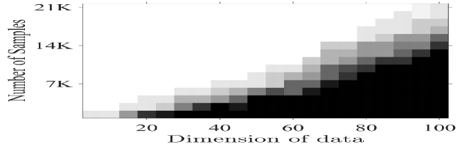
Figure 2: The sample complexity when the feature dimension changes

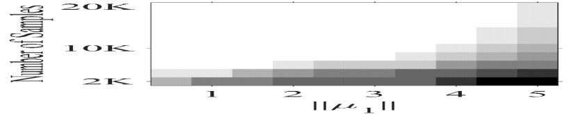
Figure 3: The sample complexity (a) when one mean changes, (b) when one co-variance changes.

We next study the impact on the sample complexity of the GMM model. In Figure 3 (a), ${\bm{\Sigma}}_{1}={\bm{\Sigma}}_{2}={\bm{I}}$, and let ${\bm{\mu}}_{1}=\mu\cdot\bm{1}$, ${\bm{\mu}}_{2}=-\bm{1}$. $\|{\bm{\mu}}_{1}\|$ varies from $0$ to $5$. Figure 3(a) shows that when the mean increases, the sample complexity increases. In Figure 3 (b), we fix ${\bm{\mu}}_{1}=\bm{1}$, ${\bm{\mu}}_{2}=-\bm{1}$, and let ${\bm{\Sigma}}_{1}=\sigma^{2}{\bm{I}}$ and ${\bm{\Sigma}}_{2}={\bm{I}}$. $\sigma$ varies from $10^{-1}$ to $10^{1}$. The sample complexity increases both when $\|{\bm{\Sigma}}_{1}\|$ increases and when $\|{\bm{\Sigma}}_{1}\|$ approaches zero. All results match predictions in Corollary 1.

Convergence analysis. We next study the convergence rate of Algorithm 1. Figure 4(a) shows the impact of $\|{\bm{\mu}}_{l}\|$. $\lambda_{1}=\lambda_{2}=0.5$, ${\bm{\mu}}_{1}=-{\bm{\mu}}_{2}=C\cdot\bm{1}$ for a positive $C$, and ${\bm{\Sigma}}_{1}={\bm{\Sigma}}_{2}={\bm{\Lambda}}^{\top}{\bm{D}}{\bm{\Lambda}}$. Here ${\bm{\Lambda}}$ is generated by computing the left-singular vectors of a $d\times d$ random matrix from the Gaussian distribution. ${\bm{D}}=\text{diag}(1,1.1,1.2,1.3,1.4)$. $n=1\times 10^{4}$. Algorithm 1 always converges linearly when $\|{\bm{\mu}}_{1}\|$ changes. Moreover, as $\|{\bm{\mu}}_{1}\|$ increases, Algorithm 1 converges slower. Figure 4 (b) shows the impact of the variance of the Gaussian mixture model. $\lambda_{1}=\lambda_{2}=0.5$, ${\bm{\mu}}_{1}=\bm{1}$, ${\bm{\mu}}_{2}=-\bm{1}$, ${\bm{\Sigma}}_{1}={\bm{\Sigma}}_{2}={\bm{\Sigma}}=\sigma^{2}\cdot{\bm{\Lambda}}^{\top}{\bm{D}}{\bm{\Lambda}}$. $n=5\times 10^{4}$. We change $\|{\bm{\Sigma}}\|$ by changing $\sigma$. Among the values we test, Algorithm 1 converges fastest when $\|{\bm{\Sigma}}\|=1$. The convergence rate slows down when $\|{\bm{\Sigma}}\|$ increases or decreases from 1. All results are consistent with the predictions in Corollary 1. We then study the impact of $K$ on the convergence rate. $\lambda_{1}=\lambda_{2}=0.5$, ${\bm{\mu}}_{1}=\bm{1}$, ${\bm{\mu}}_{2}=-\bm{1}$, ${\bm{\Sigma}}_{1}={\bm{\Sigma}}_{2}={\bm{I}}$. Figure 5 (a) shows that, as predicted by (9), the convergence rate is linear in $-1/K^{2}$.

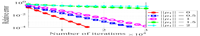
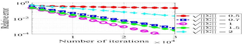
Figure 4: (a) The convergence rate with different ${\bm{\mu}}_{1}$. (b) The convergence rate with different ${\bm{\Sigma}}$. (c) Convergence rate when the number of neurons $K$ changes.

Average and group-level generalization performance. The distance between $\widehat{{\bm{W}}}_{n}$ returned by Algorithm 1 and ${\bm{W}}^{*}$ is measured by $||\widehat{{\bm{W}}}_{n}-{\bm{W}}^{*}||_{F}$. $n$ ranges from $2\times 10^{3}$ to $6\times 10^{4}$. ${\bm{\Sigma}}_{1}={\bm{\Sigma}}_{2}=9{\bm{I}}$, ${\bm{\mu}}_{1}=\bm{1}$, ${\bm{\mu}}_{2}=-\bm{1}$. Each point in Figure 5 (b) is averaged over $20$ experiments of different ${\bm{W}}^{*}$ and training set. The error is indeed linear in $\sqrt{\log(n)/n}$, as predicted by (8).

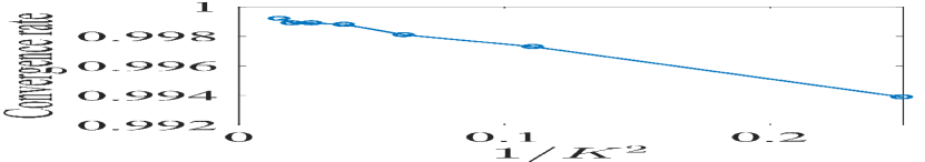
Figure 5: (a) Convergence rate when the number of neurons $K$ changes. (b) The relative error of the learned model when $n$ changes.

We evaluate the impact of one mean/co-variance of the minority group on the generalization. $n=2\times 10^{4}$. Let $\lambda_{1}=0.8$, $\lambda_{2}=0.2$, ${\bm{\mu}}_{1}=2\cdot\bm{1}$, ${\bm{\Sigma}}_{1}={\bm{I}}$. First, we let ${\bm{\mu}}_{2}=(\mu_{2}-2)\cdot\bm{1}$ and ${\bm{\Sigma}}_{2}={\bm{I}}$. Figure 6 (b) shows that both the average risk and the group-$2$ risk increase as $\mu_{2}$ increases, consistent with (P5). Then we set ${\bm{\mu}}_{2}=-2\cdot\bm{1}$, ${\bm{\Sigma}}_{2}=\sigma_{2}^{2}\cdot{\bm{I}}$. Figure 6 (a) indicates that both the average and the group-$2$ risk will first decrease and then increase as $\|\Sigma\|_{2}$ increases, consistent with (P3).

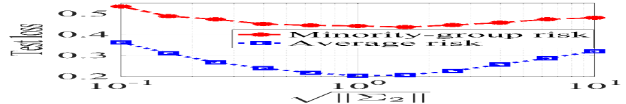
Figure 6: (a) The cross-entropy test loss when the co-variance of the minority group changes. (b) The cross-entropy test loss when the mean of the minority group changes.

Next, we study the impact of increasing the fraction of the minority group. ${\bm{\mu}}_{1}={\bm{\mu}}_{2}=0$. Let group 2 be the minority group. In Figure 7 (a), ${\bm{\Sigma}}_{1}=10\cdot{\bm{I}}$ and ${\bm{\Sigma}}_{2}={\bm{I}}$, the minority group has a smaller level of co-variance. Then when $\lambda_{2}$ increases from 0 to 0.5, both the average and group-$2$ risk decease. In Figure 7 (b), ${\bm{\Sigma}}_{1}={\bm{I}}$ and ${\bm{\Sigma}}_{2}=10\cdot{\bm{I}}$, and the minority group has a higher-level of co-variance. Then when $\lambda_{2}$ increases from 0 to 0.3, both the average and group-$2$ risk increase. As predicted by insight (P4), increasing $\lambda_{2}$ does not necessarily improve the generalization of group $2$.

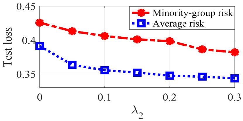
Figure 7: The test loss (cross entropy loss) of synthetic data with different $\lambda_{2}$ values. (a) Group 2 has a smaller level of co-variance. (b) Group 2 has a larger level of co-variance.

V-B Image classification on dataset CelebA

We choose the attribute “blonde hair” as the binary classification label. ResNet 9 [77] is selected to be the learning model here because it was applied in many simple computer vision tasks [78, 79]. To study the impact of co-variance, we pick $4000$ female (majority) and $1000$ male (minority) images and implement Gaussian data augmentation to create additional $300$ images for the male group. Specifically, we select $300$ out of $1000$ male images and add i.i.d. noise drawn from $\mathcal{N}(0,\delta^{2})$ to every entry. The test set includes $500$ male and $500$ female images. Figure 1 shows that when $\delta^{2}$ increases, i.e., when the co-variance of the minority group increases, both the minority-group and average test accuracy increase first and then decrease, coinciding with our insight (P3).

Then we fix the total number of training data to be $5000$ and vary the fractions of the two groups. From Figure 8(a) and (b), we observe opposite trends if we increase the fraction of the minority group in the training data with the male being the minority and the female being the minority. The norm of covariance of the male and female group in the feature space is $5.1833$ and $4.9716$, respectively. This is consistent with Insight (P4). Due to space limit, our results on the CIFAR10 dataset are deferred to Section A in the supplementary material.

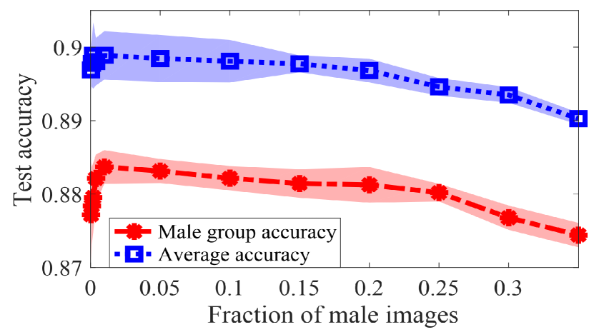
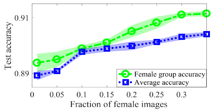
Figure 8: The test accuracy on CelebA dataset has opposite trends when the minority group fraction increases. (a) Male group is the minority (b) Female group is the minority

VI Conclusions and Future Directions

This paper provides a novel theoretical framework for characterizing neural network generalization with group imbalance. The group imbalance is formulated using the Gaussian mixture model. This paper explicitly quantifies the impact of each group on the sample complexity, convergence rate, and the average and the group-level generalization. The learning performance is enhanced when the group-level covariance is at a medium regime, and the group-level mean is close to zero. Moreover, increasing the fraction of minority group does not guarantee improved group-level generalization.

One future direction is to extend the analysis to multiple-hidden-layer neural networks and multi-class classification. Because of the concatenation of nonlinear activation functions, the analysis of the landscape of the empirical risk and the design of a proper initialization is more challenging and requires the development of new tools. Another future direction is to analyze other robust training methods, such as DRO. We see no ethical or immediate negative societal consequence of our work.

VII Acknowledgments

This research is supported in part by NSF 1932196, AFOSR FA9550-20-1-0122, and Rensselaer-IBM AI Research Collaboration (http://airc.rpi.edu), part of the IBM AI Horizons Network (http://ibm.biz/AIHorizons).

-A Definitions

Definition 1.

($\rho$-function). Let ${\bm{z}}\sim\mathcal{N}({\bm{u}},{\bm{I}}_{d})\in\mathbb{R}^{d}$. Define $\alpha_{q}(i,{\bm{u}},\sigma)=\mathbb{E}_{z_{i}\sim\mathcal{N}(u_{i},1)}[\phi^{\prime}(\sigma\cdot z_{i})z_{i}^{q}]$ and $\beta_{q}(i,{\bm{u}},\sigma)=\mathbb{E}_{z_{i}\sim\mathcal{N}(u_{i},1)}[\phi^{\prime 2}(\sigma\cdot z_{i})z_{i}^{q}]$, $\forall\ q\in\{0,1,2\}$, where $z_{i}$ and $u_{i}$ is the $i$-th entry of ${\bm{z}}$ and ${\bm{u}}$, respectively. Define $\rho({\bm{u}},\sigma)$ as

$$\rho({\bm{u}},\sigma)=\min_{i,j\in[d],j\neq i}\{ (u_{j}^{2}+1)(\beta_{0}(i,{\bm{u}},\sigma)-\alpha_{0}(i,{\bm{u}},\sigma)^{2}),$$ (13)

$$\beta_{2}(i,{\bm{u}},\sigma)-\frac{\alpha_{2}(i,{\bm{u}},\sigma)^{2}}{u_{i}^{2}+1}\}$$

Definition 2.

(D-function). Given the Gaussian Mixture Model and any positive integer $m$, define $D_{m}(\Psi)$ as

$$D_{m}(\Psi)=\sum_{l=1}^{L}\lambda_{l}(\frac{\|{{\bm{\mu}}}_{l}\|}{\|{\bm{\Sigma}}_{l}^{-1}\|^{-\frac{1}{2}}}+1)^{m},$$ (14)

$\rho$-function is defined to compute the lower bound of the Hessian of the population risk with Gaussian input. $D$-function is a normalized parameter for the means and variances. It is lower bounded by 1. $D$-function is an increasing function of $\|{\bm{\mu}}_{l}\|$ and a decreasing function of $\sigma_{l}$.

-B Proof of Lemma 1

We first restate the formal version of Lemma 1 in the following.

Lemma 1.

(Strongly local convexity) Consider the classification model with FCN (1) and the sigmoid activation function. There exists a constant $C$ such that as long as the sample size

$$n\geq C_{1}\epsilon_{0}^{-2}\cdot\big{(}\sum_{l=1}^{L}\lambda_{l}(\|{\bm{\mu}}_{l}\|+\|{\bm{\Sigma}}_{l}^{\frac{1}{2}}\|)^{2}\big{)}^{2}$$ (15)

$$\cdot\Big{(}\sum_{l=1}^{L}\lambda_{l}\frac{\|{\bm{\Sigma}}_{l}^{-1}\|^{-1}}{\eta\tau^{K}\kappa^{2}}\rho(\frac{{{\bm{W}}^{*}}^{\top}{\bm{\mu}}_{l}}{\delta_{K}({\bm{W}}^{*})\|{\bm{\Sigma}}_{l}^{-1}\|^{-\frac{1}{2}}},$$

$$\delta_{K}({\bm{W}}^{*})\|{\bm{\Sigma}}_{l}^{-1}\|^{-\frac{1}{2}})\Big{)}^{-2}dK^{5}\log^{2}{d}$$

for some constant $C_{1}>0$, $\epsilon_{0}\in(0,\frac{1}{4})$, and any fixed permutation matrix ${\bm{P}}\in\mathbb{R}^{K\times K}$ we have for all ${\bm{W}}\in\mathbb{B}({\bm{W}}^{*}{\bm{P}},r)$,

$$\Omega\Big{(}\frac{1-2\epsilon_{0}}{K^{2}}\sum_{l=1}^{L}\lambda_{l}\frac{\|{\bm{\Sigma}}_{l}^{-1}\|^{-1}}{\eta\tau^{K}\kappa^{2}}\rho(\frac{{{\bm{W}}^{*}}^{\top}{\bm{\mu}}_{l}}{\delta_{K}({\bm{W}}^{*})\|{\bm{\Sigma}}_{l}^{-1}\|^{-\frac{1}{2}}},$$ (16)

$$\delta_{K}({\bm{W}}^{*})\|{\bm{\Sigma}}_{l}^{-1}\|^{-\frac{1}{2}})\Big{)}\cdot{\bm{I}}_{dK}$$

$$\preceq\nabla^{2}f_{n}({\bm{W}})\preceq C_{2}\sum_{l=1}^{L}\lambda_{l}(||\tilde{{\bm{\mu}}}_{l}||_{\infty}+\|{\bm{\Sigma}}_{l}^{\frac{1}{2}}\|)^{2}\cdot{\bm{I}}_{dK}$$

with probability at least $1-d^{-10}$ for some constant $C_{2}>0$.

-B1 Useful lemmas

Lemmas 4, 5, 6, 7, and 8 are required for the proof.

Lemma 4.

$$\mathbb{E}_{{\bm{x}}\sim\frac{1}{2}\mathcal{N}({\bm{\mu}},{\bm{I}}_{d})+\frac{1}{2}\mathcal{N}(-{\bm{\mu}},{\bm{I}}_{d})}\Big{[}(\sum_{i=1}^{k}{\bm{r}}_{i}^{\top}{\bm{x}}\cdot\phi^{\prime}(\sigma\cdot x_{i}))^{2}\Big{]}$$ (17)

$$\geq\rho({\bm{\mu}},\sigma)||{\bm{R}}||_{F}^{2},$$

where $\rho({\bm{\mu}},\sigma)$ is defined in Definition 1 and ${\bm{R}}=({\bm{r}}_{1},\cdots,{\bm{r}}_{k})\in\mathbb{R}^{d\times k}$ is an arbitrary matrix.

Lemma 5.

With the FCN model (1) and the Gaussian Mixture Model, for any permutation matrix ${\bm{P}}$, for some constant $C_{12}>0$, we have we have

$$\mathbb{E}_{{\bm{x}}\sim\sum_{l=1}^{L}\lambda_{l}\mathcal{N}({\bm{\mu}}_{l},{\bm{\Sigma}}_{l})}\Big{[}\sup_{{\bm{W}}\neq{\bm{W}}^{\prime}\in\mathbb{B}({\bm{W}}^{*}{\bm{P}},r)}||\nabla^{2}\ell({\bm{W}},{\bm{x}})$$ (18)

$$-\nabla^{2}\ell({\bm{W}}^{\prime},{\bm{x}})||/||{\bm{W}}-{\bm{W}}^{\prime}||_{F}\Big{]}$$

$$\lesssim d^{\frac{3}{2}}K^{\frac{5}{2}}\sqrt{\sum_{l=1}^{L}\lambda_{l}(\|{\bm{\mu}}_{l}\|_{\infty}+\|{\bm{\Sigma}}_{l}\|)^{2}\sum_{l=1}^{L}\lambda_{l}(\|{\bm{\mu}}_{l}\|_{\infty}+\|{\bm{\Sigma}}_{l}\|)^{4}}$$

Lemma 6.

(Hessian smoothness of population loss) In the FCN model (1), for any permutation matrix ${\bm{P}}$, we have

$$||\nabla^{2}\bar{f}({\bm{W}})-\nabla^{2}\bar{f}({\bm{W}}^{*}{\bm{P}})||\lesssim K^{\frac{3}{2}}\cdot||{\bm{W}}-{\bm{W}}^{*}{\bm{P}}||_{F}$$ (19)

$$\cdot\Big{(}\sum_{l=1}^{L}\lambda_{l}(\|{\bm{\mu}}_{l}\|+\|{\bm{\Sigma}}_{l}^{\frac{1}{2}}\|)^{4}\sum_{l=1}^{L}\lambda_{l}(\|{\bm{\mu}}_{l}\|+\|{\bm{\Sigma}}_{l}^{\frac{1}{2}}\|)^{8}\Big{)}^{\frac{1}{4}}$$

Lemma 7.

(Local strong convexity of population loss) In the FCN model $(\ref{cla_model})$, for any permutation matrix ${\bm{P}}$, if $||{\bm{W}}-{\bm{W}}^{*}{\bm{P}}||_{F}\leq r$ for an $\epsilon_{0}\in(0,\frac{1}{4})$, then,

$$\frac{4(1-\epsilon_{0})}{K^{2}}\sum_{l=1}^{L}\lambda_{l}\frac{\|{\bm{\Sigma}}_{l}^{-1}\|^{-1}}{\eta\tau^{K}\kappa^{2}}\rho(\frac{{{\bm{W}}^{*}}^{\top}{\bm{\mu}}_{l}}{\delta_{K}({\bm{W}}^{*})\|{\bm{\Sigma}}_{l}^{-1}\|^{-\frac{1}{2}}},\delta_{K}({\bm{W}}^{*})$$ (20)

$$\cdot\|{\bm{\Sigma}}_{l}^{-1}\|^{-\frac{1}{2}})\cdot{\bm{I}}_{dK}\preceq\nabla^{2}\bar{f}({\bm{W}})\preceq\sum_{l=1}^{L}\lambda_{l}(\|{\bm{\mu}}_{l}\|+{\bm{\Sigma}}_{l}^{\frac{1}{2}})^{2}\cdot{\bm{I}}_{dK}$$

Lemma 8.

In the FCN model $(\ref{cla_model})$, for any permutation matrix ${\bm{P}}$, as long as $n\geq C^{\prime}\cdot dK\log{dK}$ for some constant $C^{\prime}>0$, we have

$$\sup_{{\bm{W}}\in\mathbb{B}({\bm{W}}^{*}{\bm{P}},r)}||\nabla^{2}f_{n}({\bm{W}})-\nabla^{2}\bar{f}({\bm{W}})||$$ (21)

$$\leq \sum_{l=1}^{L}\lambda_{l}(\|{\bm{\mu}}_{l}\|+\|{\bm{\Sigma}}_{l}^{\frac{1}{2}}\|)^{2}\sqrt{\frac{dK\log{n}}{n}})$$

with probability at least $1-d^{-10}$.

We next show the proof of Lemma 1.

-B2 Proof

From Lemma 7 and 8, with probability at least $1-d^{-10}$,

$$\nabla^{2}f_{n}({\bm{W}}) \succeq\nabla^{2}\bar{f}({\bm{W}})-||\nabla^{2}\bar{f}({\bm{W}})-\nabla^{2}f_{n}({\bm{W}})||\cdot{\bm{I}}$$ (22)

$$\succeq\Omega\Big{(}\frac{(1-\epsilon_{0})}{K^{2}}\sum_{l=1}^{L}\lambda_{l}\frac{\|{\bm{\Sigma}}_{l}^{-1}\|^{-1}}{\eta\tau^{K}\kappa^{2}}\rho(\frac{{{\bm{W}}^{*}}^{\top}{\bm{\mu}}_{l}}{\delta_{K}({\bm{W}}^{*})\|{\bm{\Sigma}}_{l}^{-1}\|^{-\frac{1}{2}}},$$

$$\delta_{K}({\bm{W}}^{*})\|{\bm{\Sigma}}_{l}^{-1}\|^{-\frac{1}{2}})\Big{)}\cdot{\bm{I}}$$

$$-O\Big{(}C_{6}\cdot\sum_{l=1}^{L}\lambda_{l}(\|{\bm{\mu}}_{l}\|+\|{\bm{\Sigma}}_{l}^{\frac{1}{2}}\|)^{2}\sqrt{\frac{dK\log{n}}{n}}\Big{)}\cdot{\bm{I}}$$

As long as the sample complexity is set to satisfy

$$\sum_{l=1}^{L}\lambda_{l}(\|{\bm{\mu}}_{l}\|+\|{\bm{\Sigma}}_{l}^{\frac{1}{2}}\|)^{2}\cdot\sqrt{\frac{dK\log{n}}{n}}\leq\frac{\epsilon_{0}}{K^{2}}\sum_{l=1}^{L}\lambda_{l}\frac{\|{\bm{\Sigma}}_{l}^{-1}\|^{-1}}{\eta\tau^{K}\kappa^{2}}$$ (23)

$$\cdot\rho(\frac{{{\bm{W}}^{*}}^{\top}{\bm{\mu}}_{l}}{\delta_{K}({\bm{W}}^{*})\|{\bm{\Sigma}}_{l}^{-1}\|^{-\frac{1}{2}}},\delta_{K}({\bm{W}}^{*})\|{\bm{\Sigma}}_{l}^{-1}\|^{-\frac{1}{2}})\cdot{\bm{I}}$$

i.e.,

$$n\gtrsim \epsilon_{0}^{-2}\cdot\big{(}\sum_{l=1}^{L}\lambda_{l}(\|{\bm{\mu}}_{l}\|+\|{\bm{\Sigma}}_{l}^{\frac{1}{2}}\|)^{2}\big{)}^{2}$$ (24)

$$\cdot\Big{(}\sum_{l=1}^{L}\lambda_{l}\frac{\|{\bm{\Sigma}}_{l}^{-1}\|^{-1}}{\eta\tau^{K}\kappa^{2}}\rho(\frac{{{\bm{W}}^{*}}^{\top}{\bm{\mu}}_{l}}{\delta_{K}({\bm{W}}^{*})\|{\bm{\Sigma}}_{l}^{-1}\|^{-\frac{1}{2}}},$$

$$\delta_{K}({\bm{W}}^{*})\|{\bm{\Sigma}}_{l}^{-1}\|^{-\frac{1}{2}})\cdot{\bm{I}}\Big{)}^{-2}dK^{5}\log^{2}{d}$$

for some constant $C_{1}>0$, then we have the lower bound of the Hessian with probability at least $1-d^{-10}$.

$$\nabla^{2}f_{n}({\bm{W}})\succeq\Omega\Big{(}\frac{1-2\epsilon_{0}}{K^{2}}\sum_{l=1}^{L}\lambda_{l}\frac{\|{\bm{\Sigma}}_{l}^{-1}\|^{-1}}{\eta\tau^{K}\kappa^{2}}$$ (25)

$$\cdot\rho(\frac{{{\bm{W}}^{*}}^{\top}{\bm{\mu}}_{l}}{\delta_{K}({\bm{W}}^{*})\|{\bm{\Sigma}}_{l}^{-1}\|^{-\frac{1}{2}}},\delta_{K}({\bm{W}}^{*})\|{\bm{\Sigma}}_{l}^{-1}\|^{-\frac{1}{2}})\Big{)}\cdot{\bm{I}}$$

By (20) and (21), we can also derive the upper bound as follows,

$$||\nabla^{2}f_{n}({\bm{W}})|| \leq||\nabla^{2}\bar{f}({\bm{W}})||+||\nabla^{2}f_{n}({\bm{W}})-\nabla^{2}\bar{f}({\bm{W}})||$$ (26)

$$\lesssim\sum_{l=1}^{L}\lambda_{l}(\|{\bm{\mu}}_{l}\|+\|{\bm{\Sigma}}_{l}^{\frac{1}{2}}\|)^{2}$$

$$+\sum_{1=1}\lambda_{l}(\|{\bm{\mu}}_{l}\|+\|{\bm{\Sigma}}_{l}^{\frac{1}{2}}\|)^{2}\sqrt{\frac{dK\log{n}}{n}}$$

$$\lesssim\sum_{l=1}^{L}\lambda_{l}(\|{\bm{\mu}}_{l}\|+\|{\bm{\Sigma}}_{l}^{\frac{1}{2}}\|)^{2}$$

Combining (25) and (26), we have

$$\Omega\Big{(}\frac{1-2\epsilon_{0}}{K^{2}}\sum_{l=1}^{L}\lambda_{l}\frac{\|{\bm{\Sigma}}_{l}^{-1}\|^{-1}}{\eta\tau^{K}\kappa^{2}}\rho(\frac{{{\bm{W}}^{*}}^{\top}{\bm{\mu}}_{l}}{\delta_{K}({\bm{W}}^{*})\|{\bm{\Sigma}}_{l}^{-1}\|^{-\frac{1}{2}}},$$ (27)

$$\delta_{K}({\bm{W}}^{*})\|{\bm{\Sigma}}_{l}^{-1}\|^{-\frac{1}{2}})\Big{)}\cdot{\bm{I}}\preceq\nabla^{2}f_{n}({\bm{W}})$$

$$\preceq \sum_{l=1}^{L}\lambda_{l}(||\tilde{{\bm{\mu}}}_{l}||_{\infty}+\|{\bm{\Sigma}}_{l}^{\frac{1}{2}}\|)^{2}\cdot{\bm{I}}$$

with probability at least $1-d^{-10}$.

-C Proof of Lemma 2

We restate the formal version of Lemma 2 in the following.

Lemma 2.

(Linear convergence of gradient descent) Assume the conditions in Lemma 1 hold. Given any fixed permutation matrix ${\bm{P}}\in\mathbb{R}^{K\times K}$, if the local convexity of $\mathbb{B}({\bm{W}}^{*}{\bm{P}},r)$ holds, there exists a critical point in $\mathbb{B}({\bm{W}}^{*}{\bm{P}},r)$ for some constant $C_{3}>0$, and $\epsilon_{0}\in(0,\frac{1}{2})$, such that

$$||\widehat{{\bm{W}}}_{n}-{\bm{W}}^{*}{\bm{P}}||_{F}$$ (28)

$$\lesssim \frac{K^{\frac{5}{2}}\sqrt{\sum_{l=1}^{L}\lambda_{l}(\|{\bm{\mu}}_{l}\|+\|{\bm{\Sigma}}_{l}^{\frac{1}{2}}\|)^{2}}(1+\xi)\cdot\sqrt{d\log{n}/n}}{\sum_{l=1}^{L}\lambda_{l}\frac{\|{\bm{\Sigma}}_{l}^{-1}\|^{-1}}{\eta\tau^{K}\kappa^{2}}\rho(\frac{{{\bm{W}}^{*}}^{\top}{\bm{\mu}}_{l}}{\delta_{K}({\bm{W}}^{*})\|{\bm{\Sigma}}_{l}^{-1}\|^{-\frac{1}{2}}},\delta_{K}({\bm{W}}^{*})\|{\bm{\Sigma}}_{l}^{-1}\|^{-\frac{1}{2}})}$$

If the initial point ${\bm{W}}_{0}\in\mathbb{B}({\bm{W}}^{*}{\bm{P}},r)$, the gradient descent linearly converges to $\widehat{{\bm{W}}}_{n}$, i.e.,

$$||{\bm{W}}_{t}-\widehat{{\bm{W}}}_{n}||_{F}\leq||{\bm{W}}_{0}-\widehat{{\bm{W}}}_{n}||_{F}\cdot\Big{(}1-$$ (29)

$$\Omega\big{(}\frac{\sum_{l=1}^{L}\frac{\lambda_{l}\|{\bm{\Sigma}}_{l}^{-1}\|^{-1}}{\eta\tau^{K}\kappa^{2}}\rho(\frac{{{\bm{W}}^{*}}^{\top}{\bm{\mu}}_{l}}{\delta_{K}({\bm{W}}^{*})\|{\bm{\Sigma}}_{l}^{-1}\|^{-\frac{1}{2}}},\delta_{K}({\bm{W}}^{*})\|{\bm{\Sigma}}_{l}^{-1}\|^{-\frac{1}{2}})}{K^{2}\sum_{l=1}^{L}\lambda_{l}(\|{\bm{\mu}}_{l}\|+\|{\bm{\Sigma}}_{l}^{\frac{1}{2}}\|)^{2}}\big{)}\Big{)}^{t}$$

with probability at least $1-d^{-10}$.

-C1 A useful lemma

Lemma 9.

If $r$ is defined in (139) for some constant $C_{3}>0$ and $\epsilon_{0}\in(0,\frac{1}{4})$, then with probability at least $1-d^{-10}$, we have

$$\sup_{{\bm{W}}\in\mathbb{B}({\bm{W}}^{*}{\bm{P}},r)}||\nabla\tilde{f}_{n}({\bm{W}})-\nabla\tilde{f}({\bm{W}})||$$ (30)

$$\lesssim \sqrt{K\sum_{l=1}^{L}\lambda_{l}(\|{\bm{\mu}}_{l}\|+\|{\bm{\Sigma}}_{l}\|)^{2}}\sqrt{\frac{d\log{n}}{n}}(1+\xi)$$

, where ${\bm{P}}$ is a permutation matrix.

We next show the proof of Lemma 2.

-C2 Proof

Following the proof of Theorem 2 in [31], first, we have Taylor’s expansion of $f_{n}(\widehat{{\bm{W}}}_{n})$

$$f_{n}(\widehat{{\bm{W}}}_{n})= f_{n}({\bm{W}}^{*}{\bm{P}})+\left\langle\nabla\tilde{f}_{n}({\bm{W}}^{*}{\bm{P}}),\text{vec}(\widehat{{\bm{W}}}_{n}-{\bm{W}}^{*}{\bm{P}})\right\rangle$$ (31)

$$+ \frac{1}{2}\text{vec}(\widehat{{\bm{W}}}_{n}-{\bm{W}}^{*}{\bm{P}})\nabla^{2}f_{n}({\bm{W}}^{\prime})\text{vec}(\widehat{{\bm{W}}}_{n}-{\bm{W}}^{*}{\bm{P}})$$

Here ${\bm{W}}^{\prime}$ is on the straight line connecting ${\bm{W}}^{*}{\bm{P}}$ and $\widehat{{\bm{W}}}_{n}$. By the fact that $f_{n}(\widehat{{\bm{W}}}_{n})\leq f_{n}({\bm{W}}^{*}{\bm{P}})$, we have

$$\frac{1}{2}\text{vec}(\widehat{{\bm{W}}}_{n}-{\bm{W}}^{*}{\bm{P}})\nabla^{2}f_{n}({\bm{W}}^{\prime})\text{vec}(\widehat{{\bm{W}}}_{n}-{\bm{W}}^{*}{\bm{P}})$$ (32)

$$\leq \Big{|}\nabla f_{n}({\bm{W}}^{*}{\bm{P}})^{\top}\text{vec}(\widehat{{\bm{W}}}_{n}-{\bm{W}}^{*}{\bm{P}})\Big{|}$$

From Lemma 7 and Lemma 9, we have

$$\frac{4}{K^{2}}\sum_{l=1}^{L}\lambda_{l}\frac{\|{\bm{\Sigma}}_{l}^{-1}\|^{-1}}{\eta\tau^{K}\kappa^{2}}\rho(\frac{{{\bm{W}}^{*}}^{\top}{\bm{\mu}}_{l}}{\delta_{K}({\bm{W}}^{*})\|{\bm{\Sigma}}_{l}^{-1}\|^{-\frac{1}{2}}},$$ (33)

$$\delta_{K}({\bm{W}}^{*})\|{\bm{\Sigma}}_{l}^{-1}\|^{-\frac{1}{2}})||\widehat{{\bm{W}}}_{n}-{\bm{W}}^{*}{\bm{P}}||_{F}^{2}$$

$$\leq \frac{1}{2}\text{vec}(\widehat{{\bm{W}}}_{n}-{\bm{W}}^{*}{\bm{P}})\nabla^{2}f_{n}({\bm{W}}^{\prime})\text{vec}(\widehat{{\bm{W}}}_{n}-{\bm{W}}^{*}{\bm{P}})$$

and

$$\Big{|}\nabla\tilde{f}_{n}({\bm{W}}^{*}{\bm{P}})^{\top}\text{vec}(\widehat{{\bm{W}}}_{n}-{\bm{W}}^{*}{\bm{P}})\Big{|}$$ (34)

$$\leq \|\nabla\tilde{f}_{n}({\bm{W}}^{*}{\bm{P}})\|\cdot\|\widehat{{\bm{W}}}_{n}-{\bm{W}}^{*}{\bm{P}}\|_{F}$$

$$\leq (\|\nabla\tilde{f}_{n}({\bm{W}}^{*}{\bm{P}})-\nabla\tilde{f}({\bm{W}}^{*}{\bm{P}})\|+\|\nabla\tilde{f}({\bm{W}}^{*}{\bm{P}})\|)$$

$$\cdot\|\widehat{{\bm{W}}}_{n}-{\bm{W}}^{*}{\bm{P}}\|_{F}$$

$$\leq O\Big{(}\sqrt{K\sum_{l=1}^{L}\lambda_{l}(\|{\bm{\mu}}_{l}\|+\|{\bm{\Sigma}}_{l}^{\frac{1}{2}}\|)^{2}}\sqrt{\frac{d\log{n}}{n}}(1+\xi)\Big{)}$$

$$||\widehat{{\bm{W}}}_{n}-{\bm{W}}^{*}{\bm{P}}||_{F}$$

The second to last step of (34) comes from the triangle inequality, and the last step follows from the fact $\nabla\bar{f}({\bm{W}}^{*}{\bm{P}})=0$. Combining (32), (33) and (34), we have

$$||\widehat{{\bm{W}}}_{n}-{\bm{W}}^{*}{\bm{P}}||_{F}$$ (35)

$$\lesssim \frac{K^{\frac{5}{2}}\sqrt{\sum_{l=1}^{L}\lambda_{l}(\|{\bm{\mu}}_{l}\|+\|{\bm{\Sigma}}_{l}^{\frac{1}{2}}\|)^{2}}(1+\xi)\cdot\sqrt{d\log{n}/n}}{\sum_{l=1}^{L}\lambda_{l}\frac{\|{\bm{\Sigma}}_{l}^{-1}\|^{-1}}{\eta\tau^{K}\kappa^{2}}\rho(\frac{{{\bm{W}}^{*}}^{\top}{\bm{\mu}}_{l}}{\delta_{K}({\bm{W}}^{*})\|{\bm{\Sigma}}_{l}^{-1}\|^{-\frac{1}{2}}},\delta_{K}({\bm{W}}^{*})\|{\bm{\Sigma}}_{l}^{-1}\|^{-\frac{1}{2}})}$$

Therefore, we have concluded that there indeed exists a critical point $\widehat{{\bm{W}}}$ in $\mathbb{B}({\bm{W}}^{*}{\bm{P}},r)$. Then we show the linear convergence of Algorithm 1 as below. By the update rule, we have

$${\bm{W}}_{t+1}-\widehat{{\bm{W}}}_{n}$$ (36)

$$= {\bm{W}}_{t}-\eta_{0}(\nabla f_{n}({\bm{W}}_{t})+\frac{1}{n}\sum_{i=1}^{n}\nu_{i})-(\widehat{{\bm{W}}}_{n}-\eta_{0}\nabla f_{n}(\widehat{{\bm{W}}}_{n}))$$

$$= \Big{(}{\bm{I}}-\eta_{0}\int_{0}^{1}\nabla^{2}f_{n}({\bm{W}}(\gamma))\Big{)}({\bm{W}}_{t}-\widehat{{\bm{W}}}_{n})-\frac{\eta_{0}}{n}\sum_{i=1}^{n}\nu_{i}$$

where ${\bm{W}}(\gamma)=\gamma\widehat{{\bm{W}}}_{n}+(1-\gamma){\bm{W}}_{t}$ for $\gamma\in(0,1)$. Since ${\bm{W}}(\gamma)\in\mathbb{B}({\bm{W}}^{*}{\bm{P}},r)$, by Lemma 1, we have

$$H_{\min}\cdot{\bm{I}}\preceq\nabla^{2}f_{n}({\bm{W}}(\gamma))\leq H_{\max}\cdot{\bm{I}}$$ (37)

where $H_{\min}=\Omega\Big{(}\frac{1}{K^{2}}\sum_{l=1}^{L}\lambda_{l}\frac{\|{\bm{\Sigma}}_{l}^{-1}\|^{-1}}{\eta\tau^{K}\kappa^{2}}\rho(\frac{{{\bm{W}}^{*}}^{\top}{\bm{\mu}}_{l}}{\delta_{K}({\bm{W}}^{*})\|{\bm{\Sigma}}_{l}^{-1}\|^{-\frac{1}{2}}},\\ \delta_{K}({\bm{W}}^{*})\|{\bm{\Sigma}}_{l}^{-1}\|^{-\frac{1}{2}})\Big{)}$, $H_{\max}=\sum_{l=1}^{L}\lambda_{l}(\|{\bm{\mu}}_{l}\|+\|{\bm{\Sigma}}_{l}\|)^{2}$. Therefore,

$$||{\bm{W}}_{t+1}-\widehat{{\bm{W}}}_{n}||_{F}$$ (38)

$$= ||{\bm{I}}-\eta_{0}\int_{0}^{1}\nabla^{2}f_{n}({\bm{W}}(\gamma))||\cdot||{\bm{W}}_{t}-\widehat{{\bm{W}}}_{n}||_{F}+\|\frac{\eta_{0}}{n}\sum_{i=1}^{n}\nu_{i}\|_{F}$$

$$\leq (1-\eta_{0}H_{\min})||{\bm{W}}_{t}-\widehat{{\bm{W}}}_{n}||_{F}+\|\frac{\eta_{0}}{n}\sum_{i=1}^{n}\nu_{i}\|_{F}$$

By setting $\eta_{0}=\frac{1}{H_{\max}}=O\Big{(}\frac{1}{\sum_{l=1}^{L}\lambda_{l}(\|{\bm{\mu}}_{l}\|+\|{\bm{\Sigma}}_{l}\|)^{2}}\Big{)}$, we obtain

$$||\widehat{{\bm{W}}}_{t+1}-\widehat{{\bm{W}}}_{n}||_{F}\leq(1-\frac{H_{\min}}{H_{\max}})||{\bm{W}}_{t}-\widehat{{\bm{W}}}_{n}||_{F}+\frac{\eta_{0}}{n}\sum_{i=1}^{n}\|\nu_{i}\|_{F}$$ (39)

Therefore, Algorithm 1 converges linearly to the local minimizer with an extra statistical error.
By Hoeffding’s inequality in [80], we have

$$\mathbb{P}\Big{(}\frac{1}{n}\sum_{i=1}^{n}\|\nu_{i}\|_{F}\geq\sqrt{\frac{dK\log n}{n}}\xi\Big{)}\lesssim\exp(-\frac{\xi^{2}dK\log n}{dK\xi^{2}})$$ (40)

$$\lesssim d^{-10}$$

Therefore, with probability $1-d^{-10}$ we can derive

$$||\widehat{{\bm{W}}}_{t}-\widehat{{\bm{W}}}_{n}||_{F}$$ (41)

$$\leq (1-\frac{H_{\min}}{H_{\max}})^{t}||{\bm{W}}_{0}-\widehat{{\bm{W}}}_{n}||_{F}+\frac{H_{\max}\eta_{0}}{H_{\min}}\sqrt{\frac{dK\log n}{n}}\xi$$

-D Proof of Lemma 3

We first restate the formal version of Lemma 3 in the following.

Lemma 3.

(Tensor initialization) For classification model, with $D_{6}(\Psi)$ defined in Definition 2, we have that if the sample size

$$n\geq\kappa^{8}K^{4}\tau^{12}D_{6}(\Psi)\cdot d\log^{2}{d},$$ (42)

then the output ${\bm{W}}_{0}\in\mathbb{R}^{d\times K}$ satisfies

$$||{\bm{W}}_{0}-{\bm{W}}^{*}{\bm{P}}^{*}||\lesssim\kappa^{6}K^{3}\cdot\tau^{6}\sqrt{D_{6}(\Psi)}\sqrt{\frac{d\log{n}}{n}}||{\bm{W}}^{*}||$$ (43)

with probability at least $1-n^{-\Omega(\delta_{1}^{4})}$ for a specific permutation matrix ${\bm{P}}^{*}\in\mathbb{R}^{K\times K}$.

-D1 Useful lemmas

Lemmas 10, 11, 12, 13, and 14 are needed to prove Lemma 3.

Lemma 10.

Let ${\bm{Q}}_{2}$ and ${\bm{Q}}_{3}$ follow Definition 3. Let $S$ be a set of i.i.d. samples generated from the mixed Gaussian distribution $\sum_{l=1}^{L}\lambda_{l}\mathcal{N}({\bm{\mu}}_{l},{\bm{\Sigma}}_{l})$. Let $\widehat{{\bm{Q}}}_{2}$, $\widehat{{\bm{Q}}}_{3}$ be the empirical version of ${\bm{Q}}_{2}$, ${\bm{Q}}_{3}$ using data set $S$, respectively. Then with a probability at least $1-2n^{-\Omega(\delta_{1}({\bm{W}}^{*})^{4}d)}$, we have

$$||{\bm{Q}}_{2}-\widehat{{\bm{Q}}}_{2}||\lesssim\sqrt{\frac{d\log{n}}{n}}\cdot\delta_{1}({\bm{W}}^{*})^{2}\cdot\tau^{6}\sqrt{D_{2}(\Psi)D_{4}(\Psi)}$$ (44)

if the mixed Gaussian distribution is not symmetric. We also have

$$||{\bm{Q}}_{3}({\bm{I}}_{d},{\bm{I}}_{d},\bm{\alpha})-\widehat{{\bm{Q}}}_{3}({\bm{I}}_{d},{\bm{I}}_{d},\bm{\alpha})||$$ (45)

$$\lesssim \sqrt{\frac{d\log{n}}{n}}\cdot\delta_{1}({\bm{W}}^{*})^{2}\cdot\tau^{6}\sqrt{D_{2}(\Psi)D_{4}(\Psi)}$$

for any arbitrary vector $\bm{\alpha}\in\mathbb{R}^{d}$, if the mixed Gaussian distribution is symmetric.

Lemma 11.

Let ${\bm{U}}\in\mathbb{E}^{d\times K}$ be the orthogonal column span of ${\bm{W}}^{*}$. Let $\bm{\alpha}$ be a fixed unit vector and $\widehat{{\bm{U}}}\in\mathbb{R}^{d\times K}$ denote an orthogonal matrix satisfying $||{\bm{U}}{\bm{U}}^{\top}-\widehat{{\bm{U}}}\widehat{{\bm{U}}}^{\top}||\leq\frac{1}{4}$. Define ${\bm{R}}_{3}={\bm{Q}}_{3}(\widehat{{\bm{U}}},\widehat{{\bm{U}}},\widehat{{\bm{U}}})$, where ${\bm{Q}}_{3}$ is defined in Definition 3. Let $\widehat{{\bm{R}}}_{3}$ be the empirical version of ${\bm{R}}_{3}$ using data set $S$, where each sample of $S$ is i.i.d. sampled from the mixed Gaussian distribution $\sum_{l=1}^{L}\lambda_{l}\mathcal{N}({\bm{\mu}}_{l},{\bm{\Sigma}}_{l})$. Then with a probability at least $1-n^{-\Omega(\delta^{4}({\bm{W}}^{*}))}$, we have

$$||\widehat{{\bm{R}}}_{3}-{\bm{R}}_{3}||\lesssim\delta_{1}({\bm{W}}^{*})^{2}\cdot\big{(}\tau^{6}\sqrt{D_{6}(\Psi)}\big{)}\cdot\sqrt{\frac{\log{n}}{n}}$$ (46)

Lemma 12.

Let $\widehat{{\bm{Q}}}_{1}$ be the empirical version of ${\bm{Q}}_{1}$ using dataset $S$. Then with a probability at least $1-2n^{-\Omega(d)}$, we have

$$||\widehat{{\bm{Q}}}_{1}-{\bm{Q}}_{1}||\lesssim\big{(}\tau^{2}\sqrt{D_{2}(\Psi)}\big{)}\cdot\sqrt{\frac{d\log{n}}{n}}$$ (47)

Lemma 13.

([29], Lemma E.6) Let ${\bm{Q}}_{2}$, ${\bm{Q}}_{3}$ be defined in Definition 3 and $\widehat{{\bm{Q}}}_{2}$, $\widehat{{\bm{Q}}}_{3}$ be their empirical version, respectively. Let ${\bm{U}}\in\mathbb{R}^{d\times K}$ be the column span of ${\bm{W}}^{*}$. Assume $||{\bm{Q}}_{2}-\widehat{{\bm{Q}}}_{2}||\leq\frac{\delta_{K}({\bm{Q}}_{2})}{10}$ for non-symmetric distribution cases and $||{\bm{Q}}_{3}({\bm{I}}_{d},{\bm{I}}_{d},\bm{\alpha})-\widehat{{\bm{Q}}}_{3}({\bm{I}}_{d},{\bm{I}}_{d},\bm{\alpha})||\leq\frac{\delta_{K}({\bm{Q}}_{3}({\bm{I}}_{d},{\bm{I}}_{d},\bm{\alpha}))}{10}$ for symmetric distribution cases and any arbitrary vector $\bm{\alpha}\in\mathbb{R}^{d}$. Then after $T=O(\log(\frac{1}{\epsilon}))$ iterations, the output of the Tensor Initialization Method 1, $\widehat{{\bm{U}}}$, will satisfy

$$||\widehat{{\bm{U}}}\widehat{{\bm{U}}}^{\top}-{\bm{U}}{\bm{U}}^{\top}||\lesssim\frac{||\widehat{{\bm{Q}}}_{2}-{\bm{Q}}_{2}||}{\delta_{K}({\bm{Q}}_{2})}+\epsilon,$$ (48)

which implies

$$||({\bm{I}}-\widehat{{\bm{U}}}\widehat{{\bm{U}}}^{\top}){\bm{w}}_{i}^{*}||\lesssim(\frac{||{\bm{Q}}_{2}-\widehat{{\bm{Q}}}_{2}||}{\delta_{K}({\bm{Q}}_{2})}+\epsilon)||{\bm{w}}_{i}^{*}||$$ (49)

if the mixed Gaussian distribution is not symmetric. Similarly, we have

$$||\widehat{{\bm{U}}}\widehat{{\bm{U}}}^{\top}-{\bm{U}}{\bm{U}}^{\top}||\lesssim\frac{||\widehat{{\bm{Q}}}_{3}({\bm{I}}_{d},{\bm{I}}_{d},\bm{\alpha})-{\bm{Q}}_{3}({\bm{I}}_{d},{\bm{I}}_{d},\bm{\alpha})||}{\delta_{K}({\bm{Q}}_{3}({\bm{I}}_{d},{\bm{I}}_{d},\bm{\alpha}))}+\epsilon,$$ (50)

which implies

$$||({\bm{I}}-\widehat{{\bm{U}}}\widehat{{\bm{U}}}^{\top}){\bm{w}}_{i}^{*}||$$ (51)

$$\lesssim (\frac{||{\bm{Q}}_{3}({\bm{I}}_{d},{\bm{I}}_{d},\bm{\alpha})-\widehat{{\bm{Q}}}_{3}({\bm{I}}_{d},{\bm{I}}_{d},\bm{\alpha})||}{\delta_{K}({\bm{Q}}_{3}({\bm{I}}_{d},{\bm{I}}_{d},\bm{\alpha}))}+\epsilon)||{\bm{w}}_{i}^{*}||$$

if the mixed Gaussian distribution is symmetric.

Lemma 14.

([29], Lemma E.13) Let ${\bm{U}}\in\mathbb{R}^{d\times K}$ be the orthogonal column span of ${\bm{W}}^{*}$. Let $\widehat{{\bm{U}}}\in\mathbb{R}^{d\times K}$ be an orthogonal matrix such that $||{\bm{U}}{\bm{U}}^{\top}-\widehat{{\bm{U}}}\widehat{{\bm{U}}}^{\top}||\lesssim\gamma_{1}\lesssim\frac{1}{\kappa^{2}\sqrt{K}}$. For each $i\in[K]$, let $\widehat{{\bm{v}}_{i}}$ denote the vector satisfying $||\widehat{{\bm{v}}_{i}}-\widehat{{\bm{U}}}^{\top}\bar{{\bm{w}}_{i}}^{*}||\leq\gamma_{2}\lesssim\frac{1}{\kappa^{2}\sqrt{K}}$. Let ${\bm{Q}}_{1}$ be defined in Lemma 12 and $\widehat{{\bm{Q}}}_{1}$ be its empirical version. If $||{\bm{Q}}_{1}-\widehat{{\bm{Q}}}_{1}||\leq\gamma_{3}||{\bm{Q}}_{1}||\lesssim\frac{1}{4}||{\bm{Q}}_{1}||$, then we have

$$\Big{|}||{\bm{w}}_{i}^{*}||-\widehat{\alpha}_{i}\Big{|}\leq(\kappa^{4}K^{\frac{3}{2}}(\gamma_{1}+\gamma_{2})+\kappa^{2}K^{\frac{1}{2}}\gamma_{3})||{\bm{w}}_{i}^{*}||$$ (52)

We next show the proof of Lemma 3.

-D2 Proof:

By the triangle inequality, we have

$$||{\bm{w}}_{j}^{*}-\widehat{\alpha}_{j}\widehat{{\bm{U}}}\widehat{{\bm{v}}}_{j}||$$ (53)

$$= \Big{|}\Big{|}{\bm{w}}_{j}^{*}-||{\bm{w}}_{j}^{*}||\widehat{{\bm{U}}}\widehat{{\bm{v}}}_{j}+||{\bm{w}}_{j}^{*}||\widehat{{\bm{U}}}\widehat{{\bm{v}}}_{j}-\widehat{\alpha}_{j}\widehat{{\bm{U}}}\widehat{{\bm{v}}}_{j}\Big{|}\Big{|}$$

$$\leq \Big{|}\Big{|}{\bm{w}}_{j}^{*}-||{\bm{w}}_{j}^{*}||\widehat{{\bm{U}}}\widehat{{\bm{v}}}_{j}\Big{|}\Big{|}+\Big{|}\Big{|}||{\bm{w}}_{j}^{*}||\widehat{{\bm{U}}}\widehat{{\bm{v}}}_{j}-\widehat{\alpha}_{j}\widehat{{\bm{U}}}\widehat{{\bm{v}}}_{j}\Big{|}\Big{|}$$

$$\leq ||{\bm{w}}_{j}^{*}||\Big{|}\Big{|}\bar{{\bm{w}}_{j}}^{*}-\widehat{{\bm{U}}}\widehat{{\bm{v}}}_{j}\Big{|}\Big{|}+\Big{|}\Big{|}||{\bm{w}}_{j}^{*}||-\widehat{\alpha}_{j}\Big{|}\Big{|}||\widehat{{\bm{U}}}\widehat{{\bm{v}}}_{j}||$$

$$\leq ||{\bm{w}}_{j}^{*}||\Big{|}\Big{|}\bar{{\bm{w}}_{j}}^{*}-\widehat{{\bm{U}}}\widehat{{\bm{U}}}^{\top}\bar{{\bm{w}}}_{j}^{*}+\widehat{{\bm{U}}}\widehat{{\bm{U}}}^{\top}\bar{{\bm{w}}_{j}}^{*}-\widehat{{\bm{U}}}\widehat{{\bm{v}}}_{j}\Big{|}\Big{|}$$

$$+\Big{|}\Big{|}||{\bm{w}}_{j}^{*}||-\widehat{\alpha}_{j}\Big{|}\Big{|}||\widehat{{\bm{U}}}\widehat{{\bm{v}}}_{j}||$$

$$\leq \delta_{1}({\bm{W}}^{*})\Big{(}\Big{|}\Big{|}\bar{{\bm{w}}_{j}}^{*}-\widehat{{\bm{U}}}\widehat{{\bm{U}}}^{\top}\bar{{\bm{w}}_{j}}^{*}\Big{|}\Big{|}+\Big{|}\Big{|}\widehat{{\bm{U}}}^{\top}\bar{{\bm{w}}_{j}}^{*}-\widehat{{\bm{v}}}_{j}\Big{|}\Big{|}\Big{)}$$

$$+\Big{|}\Big{|}||{\bm{w}}_{j}^{*}||-\widehat{\alpha}_{j}\Big{|}\Big{|}$$

From Lemma 10, Lemma 13, $\delta_{K}({\bm{Q}}_{2})\lesssim\delta_{K}^{2}({\bm{W}}^{*})$ and $\delta_{K}({\bm{Q}}_{3}({\bm{I}}_{d},{\bm{I}}_{d},\bm{\alpha}))\lesssim\delta_{K}^{2}({\bm{W}}^{*})$ for any arbitrary vector $\bm{\alpha}\in\mathbb{R}^{d}$, we have

$$\Big{|}\Big{|}\bar{{\bm{w}}_{j}}^{*}-\widehat{{\bm{U}}}\widehat{{\bm{U}}}^{\top}\bar{{\bm{w}}_{j}}^{*}\Big{|}\Big{|}$$ (54)

$$\lesssim \frac{||{\bm{Q}}_{2}-\widehat{{\bm{Q}}}_{2}||}{\delta_{K}({\bm{Q}}_{2})}\lesssim\sqrt{\frac{d\log{n}}{n}}\cdot\frac{\delta_{1}({\bm{W}}^{*})^{2}}{\delta_{K}({\bm{W}}^{*})^{2}}\cdot\tau^{6}\sqrt{D_{2}(\Psi)D_{4}(\Psi)}$$

$$= \sqrt{\frac{d\log{n}}{n}}\cdot\kappa^{2}\cdot\tau^{6}\sqrt{D_{2}(\Psi)D_{4}(\Psi)}$$

if the mixed Gaussian distribution is not symmetric, and

$$\Big{|}\Big{|}\bar{{\bm{w}}_{j}}^{*}-\widehat{{\bm{U}}}\widehat{{\bm{U}}}^{\top}\bar{{\bm{w}}_{j}}^{*}\Big{|}\Big{|}\lesssim\frac{||{\bm{Q}}_{3}({\bm{I}}_{d},{\bm{I}}_{d},\bm{\alpha})-\widehat{{\bm{Q}}}_{3}({\bm{I}}_{d},{\bm{I}}_{d},\bm{\alpha})||}{\delta_{K}({\bm{Q}}_{3}({\bm{I}}_{d},{\bm{I}}_{d},\bm{\alpha}))}$$ (55)

$$= \sqrt{\frac{d\log{n}}{n}}\cdot\kappa^{2}\cdot\tau^{6}\sqrt{D_{2}(\Psi)D_{4}(\Psi)}$$

if the mixed Gaussian distribution is symmetric. Moreover, we have

$$\Big{|}\Big{|}\widehat{{\bm{U}}}^{\top}\bar{{\bm{w}}_{j}}^{*}-\widehat{{\bm{v}}}_{j}\Big{|}\Big{|}$$ (56)

$$\leq \frac{K^{\frac{3}{2}}}{\delta_{K}^{2}({\bm{W}}^{*})}||{\bm{R}}_{3}-\widehat{{\bm{R}}}_{3}||\lesssim\kappa^{2}\cdot\big{(}\tau^{6}\sqrt{D_{6}(\Psi)}\big{)}\cdot\sqrt{\frac{K^{3}\log{n}}{n}}$$

in which the first step is by Theorem 3 in [81], and the second step is by Lemma 11. By Lemma 14, we have

$$\Big{|}\Big{|}||{\bm{w}}_{j}^{*}||-\widehat{\alpha}_{j}\Big{|}\Big{|}\leq(\kappa^{4}K^{\frac{3}{2}}(\gamma_{1}+\gamma_{2})+\kappa^{2}K^{\frac{1}{2}}\gamma_{3})||{\bm{W}}^{*}||$$ (57)

Therefore, taking the union bound of failure probabilities in Lemmas 10, 11, and 12, we have that if the sample size $n\geq\kappa^{8}K^{4}\tau^{12}D_{6}(\Psi)\cdot d\log^{2}{d}$, then the output ${\bm{W}}_{0}\in\mathbb{R}^{d\times K}$ satisfies

$$||{\bm{W}}_{0}-{\bm{W}}^{*}||\lesssim\kappa^{6}K^{3}\cdot\tau^{6}\sqrt{D_{6}(\Psi)}\sqrt{\frac{d\log{n}}{n}}||{\bm{W}}^{*}||$$ (58)

with probability at least $1-n^{-\Omega(\delta_{1}^{4}({\bm{W}}^{*}))}$

-E Extension to Multi-Classification

We only show the analysis of binary classification in the main body of the paper due to the simplicity of presentation and highlight our major conclusions on the group imbalance. We briefly introduce how to extend our analysis on binary classification to multi-classification in this section. The main idea is to define the label as a multi-dimensional vector and apply the analysis for the binary classification case multiple times. Specifically, let $C$ be the number of classes, where $C=2^{c}$ for a positive integer $c$. The label ${\bm{y}}_{i}$ is a $c$-dimensional vector, and its $j$th entry $y_{i,j}\in\{0,1\}$ for $j\in[c]$ and $i\in[n]$. Such a formulation for the multi-classification problem can be found in [49, 82]. Then, following the binary setup, data ${\bm{x}}_{i},y_{i}$ satisfies

$$\mathbb{P}(y_{i,j}=1|{\bm{x}}_{i})=H_{j}({\bm{W}}^{*},{\bm{x}}_{i}),$$ (59)

for some unknown ground-truth neural network with unknown weights ${\bm{W}}^{*}$, where $H_{j}({\bm{W}}^{*},{\bm{x}}_{i})$ is the $j$-th entry of ${\bm{H}}({\bm{W}}^{*},{\bm{x}}_{i})\in\mathbb{R}^{c}$ with the parameter ${\bm{W}}_{j}^{*}\in\mathbb{R}^{d\times K}$.

The training process is to minimize the empirical risk function with a cross-entropy loss

$$\frac{1}{n}\sum_{i=1}^{n}\sum_{j=1}^{c}-y_{i,j}\log(H_{j}({\bm{W}},{\bm{x}}_{i}))$$ (60)

$$-(1-y_{i,j})\log(1-H_{j}({\bm{W}},{\bm{x}}_{i}))$$

$$:= \sum_{j=1}^{c}f_{n}^{(j)}({\bm{W}}).$$

Note that $f_{n}^{(j)}({\bm{W}})$ has exactly the form as (2) in our paper for the binary case. Therefore, we can apply the existing theoretical results for $f_{n}^{(j)}({\bm{W}})$ with all $j\in[c]$, and summing up all the bounds yields the theoretical results for the multi-class case.

We implement experiments on the CelebA dataset for 4-classification. The only change is that we use the combinations of two attributes, “blonde hair” and “pale skin” to generate four classes of data. All other settings are the same. The results are the following.

One can observe from Figure 9 that when the noise level $\delta^{2}$ increases, i.e., when the co-variance of the minority group increases, both the minority-group and average test accuracy increase first and then decrease, coinciding with our insight (P3). In Figure 10 (a) and (b), we can see opposite trends if we increase the fraction of the minority group in the training data, with the male being the minority or the female being the minority. Figures 9 and 10 are consistent with our findings in Figures 1 and 8, respectively.

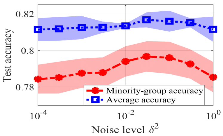
Figure 9: Test accuracy against the augmented noise level for 4-classification.

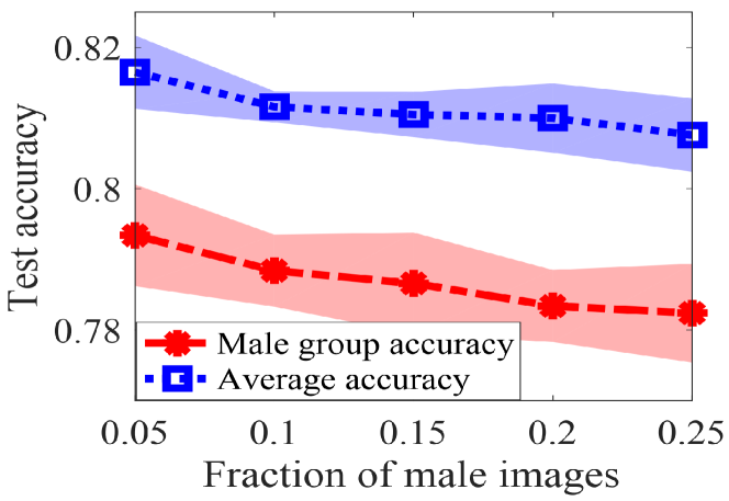
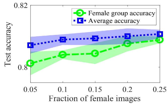
Figure 10: The test accuracy on CelebA dataset has opposite trends when the minority group fraction increases for 4-classification. (a) Male group is the minority (b) Female group is the minority

-F Discussion about Gaussian Mixture Model (GMM)

The GMM distribution intuitively means that each data comes from a certain group, which is represented by a certain Gaussian component with mean ${\bm{\mu}}_{l}$ and co-variance ${\bm{\Sigma}}_{l}$, $l\in[L]$. The fraction $\lambda_{l}$ stands for the fraction of group $l\in[L]$. This formulation is motivated by existing works [3, 26], which are related to group imbalance in the case of convolutional neural networks. One can see that each data feature follows GMM by Eqn (4) of [3]. In our setup, we define the data following the GMM for fully connected neural networks, where labels are determined by the mixture of Gaussian input and the ground-truth model.

We also conduct an experiment on CelebA to show some practical datasets satisfy the GMM model. We select data with two attributes, male and female. We extract features before the fully connected layer of the ResNet 9 model and fit the features to a two-component GMM using the EM algorithm [73]. The goodness of fit is measured by the average log-likelihood score as in [83]. We compute the average log-likelihood score of the CelebA dataset as 1.63 bits/dimension. To see that 1.63 bits/dimension reflects a good fitting, we generate synthetic data following the estimated GMM by CelebA and then compute the log-likelihood score of fitting the synthetic data to a two-component GMM. The resulting score is 1.80 bits/dimension for the synthetic two-component GMM data. Therefore, we can see that the quality of fitting CelebA is almost as good as fitting synthetic data generated by a GMM, which indicates that a two-component GMM is a good fitting for the studied practical dataset generated by CelebA.

Since many existing theoretical works [29, 31, 30, 63, 32] consider the data as standard Gaussian, we also compute the score if we use a single Gaussian to fit the data. The resulting average log-likelihood score is 1.08 bits/dimension, which is evidently smaller than the two-component GMM considered in our manuscript. This shows our GMM can better describe the real data.

Moreover, our GMM assumption goes beyond the state-of-the-art assumption of the standard Gaussian for loss landscape analysis for one-hidden-layer neural networks with convergence guarantees [29, 84, 61, 31, 32]. When generalizing from the standard Gaussian to GMM, we make new technical contributions to analyzing the more complicated and challenging landscape of the risk function because of a mixture of non-zero mean and non-unit standard deviation Gaussians. We characterize the impact of the parameters of the GMM model on the learning convergence and generalization performance. In contrast, other existing theoretical works [10, 11, 12, 85] that consider other input distributions that are more general than the standard Gaussian model do not explicitly quantify the impact of the distribution parameters on the loss landscape and generalization performance.

-G Discussion about $\sigma_{\min}$ and $\tau$

In this section, we show that the assumption that $\sigma_{\min}$ is not very close to zero, or equivalently, $\tau=\Theta(1)$, is mild. Even when the real data have singular values very close to zero, they can be approximated by low-rank data without hurting the performance by only keeping a few significant singular values and setting the small ones to zero. Thus, every practical dataset can be approximated by a dataset with $\tau=\Theta(1)$ while maintaining the same performance. We verify this by an experiment of binary classification on CelebA [35]. After training with a ResNet-9, the output feature of each testing image is $256$-dimensional. One can find that the singular value of the covariance matrix of features is close to $0$ except for the top singular values. The feature matrix reconstructed with top singular values can achieve comparable testing accuracy as using all singular values, as shown in Table II. One can observe that the feature matrix reconstruction with top-$5$ singular values, which is $2\%$ of all the singular vectors, leads to a test accuracy already close to that using all singular vectors, and the performance gap is smaller than $4.5\%$. We can compute that $\tau=4.6155=\Theta(1)$ for the feature matrix reconstructed by top $5$ singular values.

TABLE II: Testing accuracy with a reconstructed feature matrix using different amounts of singular values (s.v.)

Reconstruct with	top $5$ s.v.	top $25$ s.v.	all $256$ s.v.
Accuracy	$84.00\%$	$85.00\%$	$88.50\%$

Hongkang Li (Student Member, IEEE) received the B.E. degree in the Department of Electronic Engineering and Information Science from the University of Science and Technology of China, Hefei, China, in 2019. He is currently a Ph.D. student in the Department of Electrical, Computer, and Systems Engineering at Rensselaer Polytechnic Institute, Troy, NY, USA. His research interests include machine learning, deep learning theory, and graph neural network.

Shuai Zhang (Member, IEEE) received the B.E. degree from the University of Science and Technology of China, Hefei, China, in 2016. He received his Ph.D. degree from Rensselaer Polytechnic Institute, Troy, NY, USA, in 2021. He is currently an Assistant Professor in the Department of Data Science at New Jersey Institute of Technology, Newark, NJ, USA. Before that, he was a Postdoctoral Research Associate at Rensselaer Polytechnic Institute in 2022-2023. His research interests span deep learning, optimization, data science, and signal processing, with a particular emphasis on learning theory, algorithmic foundations of machine learning, and the development of efficient and trustworthy AI.

Yihua Zhang received the B.E. degree in the School of Mechanical Engineering at Huazhong University of Science and Technology, Wuhan, China, in 2019. He is a Ph.D. student in the Department of Computer Science and Engineering at Michigan State University. His research has been focused on the optimization theory and optimization foundations of various AI applications. In general, his research spans the areas of machine learning (ML)/deep learning (DL), computer vision, and trustworthiness. He has published papers at major ML/AI conferences such as CVPR, NeurIPS, ICLR, and ICML. He also received the Best Paper Runner-Up Award at the Conference on Uncertainty in Artificial Intelligence (UAI), 2022.

Meng Wang (Senior Member, IEEE) received B.S. and M.S. degrees from Tsinghua University, China, in 2005 and 2007, respectively. She received the Ph.D. degree from Cornell University, Ithaca, NY, USA, in 2012. She is an Associate Professor in the Department of Electrical, Computer, and Systems Engineering at Rensselaer Polytechnic Institute, Troy, NY, USA, where she joined in Dec. 2012. Before that, she was a postdoc scholar at Duke University, Durham, NC, USA. Her research interests include the theory of machine learning and artificial intelligence, high-dimensional data analytics, and power systems monitoring. She serves as an Associate Editor for IEEE Transactions on Signal Processing and IEEE Transactions on Smart Grid.

Sijia Liu (Senior Member, IEEE) received the Ph.D. degree (with All-University Doctoral Prize) in Electrical and Computer Engineering from Syracuse University, NY, USA, in 2016. He was a Postdoctoral Research Fellow at the University of Michigan, Ann Arbor, in 2016-2017, and a Research Staff Member at the MIT-IBM Watson AI Lab in 2018-2020. He is currently an Assistant Professor at the CSE department of Michigan State University, and an Affiliate Professor at the MIT-IBM Watson AI Lab, IBM Research. His research focuses on trustworthy and scalable ML, and optimization theory and methods. He received the Best Student Paper Award at the 42nd IEEE International Conference on Acoustics, Speech and Signal Processing (ICASSP’16), and the Best Paper Runner-Up Award at the 38th Conference on Uncertainty in Artificial Intelligence (UAI’22).

Pin-Yu Chen (Member, IEEE) Dr. Pin-Yu Chen is a principal research scientist at IBM Thomas J. Watson Research Center, Yorktown Heights, NY, USA. He is also the chief scientist of RPI-IBM AI Research Collaboration and PI of ongoing MIT-IBM Watson AI Lab projects. Dr. Chen received his Ph.D. in electrical engineering and computer science from the University of Michigan, Ann Arbor, USA, in 2016. Dr. Chen’s recent research focuses on adversarial machine learning of neural networks for robustness and safety. His long-term research vision is to build trustworthy machine learning systems. He received the IJCAI Computers and Thought Award in 2023. At IBM Research, he received several research accomplishment awards, including IBM Master Inventor, IBM Corporate Technical Award, and IBM Pat Goldberg Memorial Best Paper. His research contributes to IBM open-source libraries including Adversarial Robustness Toolbox (ART 360) and AI Explainability 360 (AIX 360). He has published more than 50 papers related to trustworthy machine learning at major AI and machine learning conferences. He is currently on the editorial board of Transactions on Machine Learning Research and serves as an Area Chair or Senior Program Committee member for NeurIPS, ICML, AAAI, IJCAI, and PAKDD.

Supplementary Material

We begin our Supplementary Material here.

Section -H provides more experiment results as a supplement of Section V.

Section -I introduces the algorithm, especially the tensor initialization in detail.

Section -J includes some definitions and properties as a preliminary to our proof.

Section -K shows the proof of Theorem 1 and Corollary 1, followed by Section -L, -M, and -N as the proof of three key Lemmas about local convexity, linear convergence and tensor initialization, respectively.

-H More Experiment Results

We present our experiment resultson empirical datasets CelebA [35] and CIFAR-10 in this section. To be more specific, we evaluate the impact of the variance levels introduced by different data augmentation methods on the learning performance. We also evaluate the impact of the minority group fraction in the training data on the learning performance. All the experiments are reported in a format of “mean$\pm 2\times$standard deviation” with a random seed equal to $10$. We implement our experiments on an NVIDIA GeForce RTX 2070 super GPU and a work station with 8 cores of 3.40GHz Intel i7 CPU.

-H1 Tests on CelebA

In addition to the Gaussian augmentation method in Figure 1 (b), we also evaluate the performance of data augmentation by cropping in Figure 11. The setup is exactly the same as that for Gaussian augmentation, expect that we augment the data by cropping instead of adding Gaussian noise. Specifically, to generate an augmented image, we randomly crop an image with a size $w\times w\times 3$ and then resize back to $224\times 224\times 3$. One can observe that the minority-group and average test accuracy first increase and then decrease as $w$ increases, which is in accordance with Insight (P3).

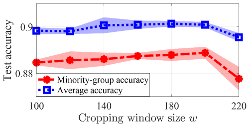
Figure 11: The test accuracy of CelebA dataset with the data augmentation method of cropping.

-H2 Tests on CIFAR-10

Group 1 contains images with attributes “bird”, “cat”, “deer”, “dog”, “frog” and “horse.” Group 2 contains “airplane” images. In this setting, Group 1 has a larger variance. Because each image in CIFAR-10 only has one attribute, we consider the binary classification setting where all images in Group 1 are labeled as “animal” and all images are labeled as “airplane.” This is a special scenario that the group label is also the classification label. Note that our results hold for general setups where group labels and classification labels are irrelevant, like our previous results on CelebA. LeNet 5 [42] is selected to be the learning model.

We first pick $8000$ animal images (majority) and $2000$ airplane images (minority). We select $1000$ out of $2000$ airplane images to implement data augmentation, including both Gaussian augmentation and random cropping. For Gaussian augmentation, we add i.i.d. Gaussian noise drawn from $\mathcal{N}(0,\delta^{2})$ to each entry. For random cropping, we randomly crop the image with a certain size $w\times w\times 3$ and then resizing back to $32\times 32\times 3$. Figure 12 shows that when $\delta$ or $w$ increase, i.e., the variance introduced by either augmentation method increases, both the minority-group and average test accuracy increase first and then decrease, which is consistent with our Insight (P3).

Then we fix the total number of training data to be $5000$ and vary the fractions of the two groups. One can see opposite trends in Figure 13 if we increase the fraction of the minority group with the airplane being the minority and the animal being the minority, which reflects our Insight (P4).

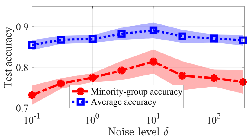
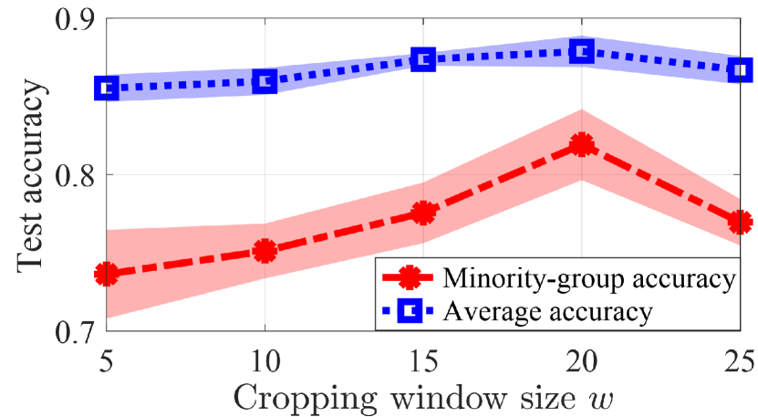
Figure 12: The test accuracy of CIFAR-10 dataset with different data augmentation methods (a) Gaussian noise (b) cropping.

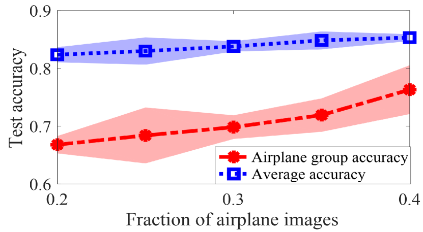
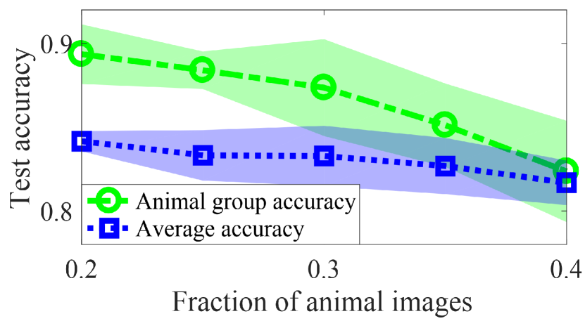
Figure 13: The test accuracy of CIFAR-10 dataset has opposite trends when the minority group fraction increases (a) Airplane group is the minority. (b) Animal group is the minority.

-I Algorithm

We first introduce new notations to be used in this part and summarize key notions in Table III.
We write $f(x)\lesssim(\gtrsim)g(x)$ if $f(x)\leq(\geq)\Theta(g(x)$. The gradient and the Hessian of a function $f({\bm{W}})$ are denoted by $\nabla f({\bm{W}})$ and $\nabla^{2}f({\bm{W}})$, respectively. ${\bm{A}}\succeq 0$ means ${\bm{A}}$ is a positive semi-definite (PSD) matrix. ${\bm{A}}^{\frac{1}{2}}$ means that ${\bm{A}}=({\bm{A}}^{\frac{1}{2}})^{2}$. The outer product of vectors ${\bm{z}}_{i}\in\mathbb{R}^{n_{i}}$, $i\in[l]$, is defined as ${\bm{T}}={\bm{z}}_{1}\otimes\cdots\otimes{\bm{z}}_{l}\in\mathbb{R}^{n_{1}\times\cdots\times n_{l}}$ with ${\bm{T}}_{j_{1}\cdots j_{l}}=({\bm{z}}_{1})_{j_{1}}\cdots({\bm{z}}_{l})_{j_{l}}$. Given a tensor ${\bm{T}}\in\mathbb{R}^{n_{1}\times n_{2}\times n_{3}}$ and matrices ${\bm{A}}\in\mathbb{R}^{n_{1}\times d_{1}}$, ${\bm{B}}\in\mathbb{R}^{n_{2}\times d_{2}}$, ${\bm{C}}\in\mathbb{R}^{n_{3}\times d_{3}}$, the $(i_{1},i_{2},i_{3})$-th entry of the tensor ${\bm{T}}({\bm{A}},{\bm{B}},{\bm{C}})$ is given by

$$\sum_{i_{1}^{\prime}}^{n_{1}}\sum_{i_{2}^{\prime}}^{n_{2}}\sum_{i_{3}^{\prime}}^{n_{3}}{\bm{T}}_{i_{1}^{\prime},i_{2}^{\prime},i_{3}^{\prime}}{{\bm{A}}}_{i_{1}^{\prime},i_{1}}{{\bm{B}}}_{i_{2}^{\prime},i_{2}}{{\bm{C}}}_{i_{3}^{\prime},i_{3}}.$$ (61)

TABLE III: Summary of notations

$\lambda_{l},\ {\bm{\mu}}_{l},\ {\bm{\Sigma}}_{l},\ l\in[L]$	The fraction, mean, and covariance of the $l$-th component in the Gaussian mixture distribution, respectively.
$d,\ n,\ K$	The feature dimension, the number of training samples, and the number of neurons, respectively.
${\bm{W}}^{*},\ {\bm{W}}_{t}$	${\bm{W}}^{*}$ is the ground truth weight. ${\bm{W}}_{t}$ is the updated weight in the $t$-th iteration.
$f_{n},\ \bar{f},\ \ell$	$f_{n}$ is the empirical risk function. $\bar{f}$ is the average risk or the population risk function. $\ell$ is the cross-entropy loss function.
$\Psi,\ \sigma_{\max},\ \sigma_{\min},\ \tau$	$\Psi$ denotes our Gaussian mixture model $(\lambda_{l},{\bm{\mu}}_{l},{\bm{\Sigma}}_{l},\forall l)$. $\sigma_{\max}=\max_{l\in[L]}\{\|{\bm{\Sigma}}_{l}\|^{\frac{1}{2}}\}$. $\sigma_{\min}=\min_{l\in[L]}\{\|{\bm{\Sigma}}_{l}^{-1}\|^{-\frac{1}{2}}\}$. $\tau=\sigma_{\max}/\sigma_{\min}$.
$\delta_{i}({\bm{W}}^{*}),\ \eta,\ \kappa,\ i\in[K]$	$\delta_{i}({\bm{W}}^{*})$ is the $i$-th largest singular value of ${\bm{W}}^{*}$. $\eta$ and $\kappa$ are two functions of ${\bm{W}}^{*}$.
$\rho({\bm{u}},\sigma),\ \Gamma(\Psi),\ D_{m}(\Psi)$	These items are functions of the Gaussian mixture distribution $\Psi$ used to develop our Theorem 1.
$\bm{\nu}_{i},\ \xi$	$\bm{\nu}_{i}$ is the gradient noise. $\xi$ is the upper bound of the noise level.
${\bm{Q}}_{j},\ j=1,2,3$	${\bm{Q}}_{j}$’s are tensors used in the initialization.
$\mathcal{B}(\Psi)$	A parameter appeared in the sample complexity bound (7).
$v(\Psi),\ q(\Psi)$	$v(\Psi)$ is the convergence rate (8). $q(\Psi)$ is a parameter in the definition of $v(\Psi)$ (9).
$\mathcal{E}_{w}(\Psi),\ \mathcal{E},\ \mathcal{E}_{l}$	Generalization parameters. $\mathcal{E}_{w}(\Psi)$ appears in the error bound of the model (10). $\mathcal{E}(\Psi)$ and $\mathcal{E}_{l}(\Psi)$ are to characterize the average risk (11) and the group-l risk (12), respectively.

The method starts from an initialization ${\bm{W}}_{0}\in\mathbb{R}^{d\times K}$ computed based on the tensor initialization method (Subroutine 1) and then updates the iterates ${\bm{W}}_{t}$ using gradient descent with the step size $\eta_{0}$. To model the inaccuracy in computing the gradient, an i.i.d. zero-mean noise $\{\nu_{i}\}_{i=1}^{n}\in\mathbb{R}^{d\times K}$ with bounded magnitude $|(\nu_{i})_{jk}|\leq\xi$ ($j\in[d],k\in[K]$) for some $\xi\geq 0$ are added in (6) when computing the gradient of the loss in (3).

Our tensor initialization method in Subroutine 1 is extended from [86] and [29]. The idea is to compute quantities (${\bm{Q}}_{j}$ in (62)) that are tensors of ${\bm{w}}^{*}_{i}$ and then apply the tensor decomposition method to estimate ${\bm{w}}^{*}_{i}$. Because ${\bm{Q}}_{j}$ can only be estimated from training samples, tensor decomposition does not return ${\bm{w}}^{*}_{i}$ exactly but provides a close approximation, and this approximation is used as the initialization for Algorithm 1. Because the existing method of tensor construction only applies to the standard Gaussian distribution, we exploit the relationship between probability density functions and tensor expressions developed in [86] to design tensors suitable for the Gaussian mixture model. Formally,

Definition 3.

For $j=1,2,3$, we define

$${\bm{Q}}_{j}:=\mathbb{E}_{{\bm{x}}\sim\sum_{l=1}^{L}\lambda_{l}\mathcal{N}({\bm{\mu}}_{l},{\bm{\Sigma}}_{l})}[y\cdot(-1)^{j}p^{-1}({\bm{x}})\nabla^{(j)}p({\bm{x}})],$$ (62)

where $p({\bm{x}})$, the probability density function of GMM is defined as

$$p(\bm{x})=\sum_{l=1}^{L}\lambda_{l}(2\pi)^{-\frac{d}{2}}|{\bm{\Sigma}}_{l}|^{-\frac{1}{2}}\exp\big{(}-\frac{1}{2}(\bm{x}-\bm{\mu}_{l}){\bm{\Sigma}}_{l}^{-1}(\bm{x}-\bm{\mu}_{l})\big{)}$$ (63)

If the Gaussian mixture model is symmetric, the symmetric distribution can be written as

$${{\bm{x}}\sim\left\{\begin{array}[]{ll}\sum\limits_{l=1}^{\frac{L}{2}}\lambda_{l}\big{(}\mathcal{N}({\bm{\mu}}_{l},{\bm{\Sigma}}_{l})+\mathcal{N}(-{\bm{\mu}}_{l},{\bm{\Sigma}}_{l})\big{)}&L\textrm{ is even}\\ \lambda_{1}\mathcal{N}(\bm{0},{\bm{\Sigma}}_{1})+\sum\limits_{l=2}^{\frac{L-1}{2}}\lambda_{l}\big{(}\mathcal{N}({\bm{\mu}}_{l},{\bm{\Sigma}}_{l})+\mathcal{N}(-{\bm{\mu}}_{l},{\bm{\Sigma}}_{l})\big{)}&L\textrm{ is odd}\end{array}\right.}$$ (64)

${\bm{Q}}_{j}$ is a $j$th-order tensor of ${\bm{w}}^{*}_{i}$, e.g., ${\bm{Q}}_{3}=\frac{1}{K}\sum_{i=1}^{K}\mathbb{E}_{{\bm{x}}\sim\sum_{l=1}^{L}\lambda_{l}\mathcal{N}({\bm{\mu}}_{l},{\bm{\Sigma}}_{l})}[\phi^{\prime\prime\prime}({{\bm{w}}_{i}^{*}}^{\top}{\bm{x}})]{{\bm{w}}_{i}^{*}}^{\otimes 3}$. These quantifies cannot be directly computed from (62) but can be estimated by sample means, denoted by $\widehat{{\bm{Q}}}_{j}$ ($j=1,2,3$), from samples $\{{\bm{x}}_{i},y_{i}\}_{i=1}^{n}$. The following assumption guarantees that these tensors are nonzero and can thus be leveraged to estimate ${\bm{W}}^{*}$.

Assumption 1.

The Gaussian Mixture Model in (64) satisfies the following conditions:

1. ${\bm{Q}}_{1}$ and ${\bm{Q}}_{3}$ are nonzero.

2. If the distribution is not symmetric, then ${\bm{Q}}_{2}$ is nonzero.

Assumption 1 is a very mild assumption. Moreover, as indicated in [86], in the rare case that some quantities ${\bm{Q}}_{i}$ ($i=1,2,3$) are zero, one can construct higher-order tensors in a similar way as in Definition 3 and then estimate ${\bm{W}}^{*}$ from higher-order tensors.

Subroutine 1 describes the tensor initialization method, which estimates the direction and magnitude of ${\bm{w}}_{j}^{*},j\in[K]$, separately. The direction vectors are denoted as $\bm{\bar{w}}_{j}^{*}={\bm{w}}_{j}^{*}/\|{\bm{w}}_{j}^{*}\|$ and the magnitude $\|{\bm{w}}_{j}^{*}\|$ is denoted as $z_{j}$. Lines 2-6 estimate the subspace $\widehat{{\bm{U}}}$ spanned by $\{{\bm{w}}_{1}^{*},\cdots,{\bm{w}}_{K}^{*}\}$ using $\widehat{{\bm{Q}}}_{2}$ or, in the case that ${\bm{Q}}_{2}=0$, a second-order tensor projected by $\widehat{{\bm{Q}}}_{3}$. Lines 7-8 estimate $\bm{\bar{w}}_{j}^{*}$ by employing the KCL algorithm [81]. Lines 9-10 estimate the magnitude $z_{j}$. Finally, the returned estimation of ${\bm{W}}^{*}$ is used as an initialization ${\bm{W}}_{0}$ for Algorithm 1. The computational complexity of Subroutine 1 is $O(Knd)$ based on similar calculations as those in [29].

Subroutine 1 Tensor Initialization Method

1:Input: Partition $n$ pairs of data $\{({\bm{x}}_{i},y_{i})\}_{i=1}^{n}$ into three disjoint subsets $\mathcal{D}_{1}$, $\mathcal{D}_{2}$, $\mathcal{D}_{3}$

2:if the Gaussian Mixture distribution is not symmetric then

3:   Compute $\widehat{{\bm{Q}}}_{2}$ using $\mathcal{D}_{1}$. Estimate the subspace $\widehat{{\bm{U}}}$ by orthogonalizing the eigenvectors with respect to the $K$ largest eigenvalues of $\widehat{{\bm{Q}}}_{2}$

4:else

5:   Pick an arbitrary vector $\bm{\alpha}\in\mathbb{R}^{d}$, and use $\mathcal{D}_{1}$ to compute $\widehat{{\bm{Q}}}_{3}({\bm{I}}_{d},{\bm{I}}_{d},\bm{\alpha})$. Estimate $\widehat{{\bm{U}}}$ by orthogonalizing the eigenvectors with respect to the $K$ largest eigenvalues of $\widehat{{\bm{Q}}}_{3}({\bm{I}}_{d},{\bm{I}}_{d},\bm{\alpha})$.

6:end if

7:Compute $\widehat{{\bm{R}}}_{3}=\widehat{{\bm{Q}}}_{3}(\widehat{{\bm{U}}},\widehat{{\bm{U}}},\widehat{{\bm{U}}})$ from data set $\mathcal{D}_{2}$

8:Employ the KCL algorithm to compute vectors $\{\hat{{\bm{v}}}_{i}\}_{i\in[K]}$, which are the estimates of $\{\widehat{{\bm{U}}}^{\top}\bm{\bar{w}}_{i}^{*}\}_{i=1}^{K}$. Then the direction vectors $\{\bm{\bar{w}}_{i}^{*}\}_{i=1}^{K}$ can be approximated by $\{\widehat{{\bm{U}}}\hat{{\bm{v}}}_{i}\}_{i=1}^{K}$.

9:Compute $\widehat{{\bm{Q}}}_{1}$ from data set $\mathcal{D}_{3}$.

10:Estimate the magnitude $\widehat{{\bm{z}}}$ by solving the optimization problem

$$\widehat{\bm{z}}=\arg\min_{\bm{\alpha}\in\mathbb{R}^{K}}\frac{1}{2}\|\widehat{{\bm{Q}}}_{1}-\sum_{j=1}^{K}\alpha_{j}\bm{\bar{w}}_{j}^{*}\|^{2}$$ (65)

11:Return: Use $\hat{z}_{j}\widehat{{\bm{U}}}\hat{{\bm{v}}}_{j}$ as the $j$th column of ${\bm{W}}_{0}$, $j\in[K]$.

-I1 Numerical Evaluation of Tensor Initialization

Figure 14 shows the accuracy of the returned model by Algorithm 1. Here $n=2\times 10^{5}$, $d=50$, $K=2$, $\lambda_{1}=\lambda_{2}=0.5$, ${\bm{\mu}}_{1}=-0.3\cdot\bm{1}$ and ${\bm{\mu}}_{2}=\bm{0}$. We compare the tensor initialization with a random initialization in a local region $\{{\bm{W}}\in\mathbb{R}^{d\times K}:||{\bm{W}}-{\bm{W}}^{*}||_{F}\leq\epsilon\}$. Each entry of ${\bm{W}}^{*}$ is selected from $[-0.1,0.1]$ uniformly. Tensor initialization in Subroutine 1 returns an initial point close to one permutation of ${\bm{W}}^{*}$, with a relative error of $0.65$. If the random initialization is also close to ${\bm{W}}^{*}$, e.g., $\epsilon=0.1$, then the gradient descent algorithm converges to a critical point from both initializations, and the linear convergence rate is the same. We also test a random initialization with each entry drawn from $\mathcal{N}(0,25)$. The initialization is sufficiently far from ${\bm{W}}^{*}$, and the algorithm does not converge. On a MacBook Pro with Intel(R) Core(TM) i5-7360U CPU at 2.30GHz and MATLAB 2017a, it takes 5.52 seconds to compute the tensor initialization. Thus, to reduce the computational time, we consider a random initialization with $\epsilon=0.1$ in the experiments instead of computing tensor initialization.

Figure 14: Comparison between tensor initialization, a random initialization near ${\bm{W}}^{*}$, and an arbitrary random initialization

-J Preliminaries of the Main Proof

In this section, we introduce some definitions and properties that will be used to prove the main results.

First, we define the sub-Gaussian random variable and sub-Gaussian norm.

Definition 4.

We say $X$ is a sub-Gaussian random variable with sub-Gaussian norm $K>0$, if $(\mathbb{E}|X|^{p})^{\frac{1}{p}}\leq K\sqrt{p}$ for all $p\geq 1$. In addition, the sub-Gaussian norm of X, denoted $\|X\|_{\psi_{2}}$, is defined as $\|X\|_{\psi_{2}}=\sup_{p\geq 1}p^{-\frac{1}{2}}(\mathbb{E}|X|^{p})^{\frac{1}{p}}$.

Then we define the following three quantities. $\rho({\bm{\mu}},\sigma)$ is motivated by the $\rho$ parameter for the standard Gaussian distribution in [29], and we generalize it to a Gaussian with an arbitrary mean and variance. We define the new quantities $\Gamma(\Psi)$ and $D_{m}(\Psi)$ for the Gaussian mixture model.

Definition 5.

($\Gamma$-function). With (13) and $\kappa$, $\eta$ defined in Section III, we define

$$\Gamma(\Psi)=\sum_{l=1}^{L}\frac{\lambda_{l}}{\tau^{K}\kappa^{2}\eta}\frac{\|{\bm{\Sigma}}_{l}^{-1}\|^{-1}}{\sigma_{\max}^{2}}\rho(\frac{{{\bm{W}}^{*}}^{\top}{\bm{\mu}}_{l}}{\delta_{K}({\bm{W}}^{*})\|{\bm{\Sigma}}_{l}^{-1}\|^{-\frac{1}{2}}},\delta_{K}({\bm{W}}^{*})\|{\bm{\Sigma}}_{l}^{-1}\|^{-\frac{1}{2}})$$ (66)

$\Gamma$ function is the weighted sum of $\rho$-function under mixture Gaussian distribution. This function is positive and upper bounded by a small value. $\Gamma$ goes to zero if all $\|{\bm{\mu}}_{l}\|$ or all $\sigma_{l}$ goes to infinity.

Property 1.

Given ${\bm{W}}^{*}={\bm{U}}{\bm{V}}\in\mathbb{R}^{d\times k}$, where ${\bm{U}}\in\mathbb{R}^{d\times K}$ is the orthogonal basis of ${\bm{W}}^{*}$. For any ${\bm{\mu}}\in\mathbb{R}^{d}$, we can find an orthogonal decomposition of ${\bm{\mu}}$ based on the colomn space of ${\bm{W}}^{*}$, i.e. ${\bm{\mu}}={\bm{\mu}}_{{\bm{U}}}+{\bm{\mu}}_{{\bm{U}}_{\perp}}$. If we consider the recovery problem of FCN with a dataset of Gaussian Mixture Model, in which ${\bm{x}}_{i}\sim\mathcal{N}({\bm{\mu}}_{h},{\bm{\Sigma}}_{h})$ for some $h\in[L]$, the problem is equivalent to the problem of FCN with ${\bm{x}}_{i}\sim\mathcal{N}({{\bm{\mu}}_{{\bm{U}}}}_{h},{\bm{\Sigma}}_{h})$. Hence, we can assume without loss of generality that ${\bm{\mu}}_{l}$ belongs to the column space of ${\bm{W}}^{*}$ for all $l\in[L]$.

Proof:
From (1) and (3), the recovery problem can be formulated as

$$\min_{{\bm{W}}^{*}}\ {g({{\bm{W}}^{*}}^{\top}{\bm{x}}_{i},y_{i})}$$

For any ${\bm{x}}_{i}\sim\mathcal{N}({\bm{\mu}}_{h},{\bm{\Sigma}}_{h})$, ${\bm{x}}_{i}$ can be written as

$${\bm{x}}_{i}={\bm{z}}+{\bm{\mu}}_{h}$$

where ${\bm{z}}\sim\mathcal{N}({\bm{0}},{\bm{\Sigma}}_{h})$. Therefore,

$${{\bm{W}}^{*}}^{\top}{\bm{x}}_{i}={{\bm{W}}^{*}}^{\top}({\bm{z}}+{\bm{\mu}}_{h})={{\bm{W}}^{*}}^{\top}({\bm{z}}+{{\bm{\mu}}_{{\bm{U}}}}_{h}+{{\bm{\mu}}_{{\bm{U}}_{\perp}}}_{h})={{\bm{W}}^{*}}^{\top}({\bm{z}}+{{\bm{\mu}}_{{\bm{U}}}}_{h})$$

The final step is because ${{\bm{W}}^{*}}^{\top}{\bm{\mu}}_{{\bm{U}}_{\perp}}={\bm{0}}$. So the problem is equivalent to the recovery problem of FCN with ${\bm{x}}_{i}\sim\mathcal{N}({{\bm{\mu}}_{{\bm{U}}}}_{h},{\bm{\Sigma}}_{h})$.

Recall that the gradient noise $\bm{\nu}_{i}\in\mathbb{R}^{d\times K}$ is zero-mean, and each of its entry is upper bounded by $\xi>0$.

Property 2.

We have that $\|\bm{\nu}_{i}\|_{F}$ is a sub-Gaussian random variable with its sub-Gaussian norm bounded bu $\xi\sqrt{dK}$.

Proof:

$$(\mathbb{E}\|\bm{\nu}_{i}\|_{F}^{p})^{\frac{1}{p}}\leq(\mathbb{E}|\sqrt{dK}\xi|^{p})^{\frac{1}{p}}\leq\xi\sqrt{dK}$$ (67)

We state some general properties of the $\rho$ function defined in Definition 1 in the following.

Property 3.

$\rho({\bm{u}},\sigma)$ in Definition 1 satisfies the following properties,

1. (Positive) $\rho({\bm{u}},\sigma)>0$ for any ${\bm{u}}\in\mathbb{R}^{d}$ and $\sigma\neq 0$.

2. (Finite limit point for zero mean) $\rho({\bm{u}},\sigma)$ converges to a positive value function of $\sigma$ as $u_{i}$ goes to 0, i.e. $\lim_{u_{i}\rightarrow 0}\rho({\bm{u}},\sigma):=\mathcal{C}_{m}(\sigma)$.

3. (Finite limit point for zero variance) When all $u_{i}\neq 0\ (i\in[d])$, $\rho(\frac{{\bm{u}}}{\sigma},\sigma)$ converges to a strictly positive real function of ${\bm{u}}$ as $\sigma$ goes to 0, i.e. $\lim_{\sigma\rightarrow 0}\rho(\frac{{\bm{u}}}{\sigma},\sigma):=\mathcal{C}_{s}({\bm{u}})$. When $u_{i}=0$ for some $i\in[d]$, $\lim_{\sigma\rightarrow 0}\rho(\frac{{\bm{u}}}{\sigma},\sigma)=0$.

4. (Lower bound function of the mean) When everything else except $|u_{i}|$ is fixed, $\rho(\frac{{{\bm{W}}^{*}}^{\top}{\bm{u}}}{\sigma\delta_{K}({\bm{W}}^{*})},\sigma\delta_{K}({\bm{W}}^{*}))$ is lower bounded by a strictly positive real function, $\mathcal{L}_{m}(\frac{({\bm{\Lambda}}{{\bm{W}}^{*}})^{\top}{\bm{\Lambda}}{\bm{u}}}{\sigma\delta_{K}({\bm{W}}^{*})},\sigma\delta_{K}({\bm{W}}^{*}))$, which is monotonically decreasing as $|u_{i}|$ increases.

5. (Lower bound function of the variance) When everything else except $\sigma$ is fixed, $\rho(\frac{{{\bm{W}}^{*}}^{\top}{\bm{u}}}{\sigma\delta_{K}({\bm{W}}^{*})},\sigma\delta_{K}({\bm{W}}^{*}))$ is lower bounded by a strictly positive real function, $\mathcal{L}_{s}(\frac{{{\bm{W}}^{*}}^{\top}{\bm{u}}}{\sigma\delta_{K}({\bm{W}}^{*})},\sigma\delta_{K}({\bm{W}}^{*}))$, which satisfies the following conditions: (a) there exists $\zeta_{s^{\prime}}>0$, such that $\sigma^{-1}\mathcal{L}_{s}(\frac{{{\bm{W}}^{*}}^{\top}{\bm{u}}}{\sigma\delta_{K}({\bm{W}}^{*})},\sigma\delta_{K}({\bm{W}}^{*}))$ is an increasing function of $\sigma$ when $\sigma\in(0,\zeta_{s^{\prime}})$; (b) there exists $\zeta_{s}>0$ such that $\mathcal{L}_{s}(\frac{{{\bm{W}}^{*}}^{\top}{\bm{u}}}{\sigma\delta_{K}({\bm{W}}^{*})},\sigma\delta_{K}({\bm{W}}^{*}))$ is a decreasing function of $\sigma$ when $\sigma\in(\zeta_{s},+\infty)$.

Proof:
(1) From Cauchy Schwarz’s inequality, we have

$$\mathbb{E}_{z_{i}\sim\mathcal{N}(u_{i},1)}[\phi^{\prime}(\sigma\cdot z_{i})]\leq\sqrt{\mathbb{E}_{z_{i}\sim\mathcal{N}(u_{i},1)}[\phi^{\prime 2}(\sigma\cdot z_{i})]}$$ (68)

$$\mathbb{E}_{z_{i}\sim\mathcal{N}(u_{i},1)}[\phi^{\prime}(\sigma\cdot z_{i})z_{i}\cdot z_{i}] \leq\sqrt{\mathbb{E}_{z_{i}\sim\mathcal{N}(u_{i},1)}[\phi^{\prime 2}(\sigma\cdot z_{i})z_{i}^{2}]}\cdot\sqrt{\mathbb{E}_{z_{i}\sim\mathcal{N}(u_{i},1)}[z_{i}^{2}]}$$ (69)

$$=\sqrt{\mathbb{E}_{z_{i}\sim\mathcal{N}(u_{i},1)}[\phi^{\prime 2}(\sigma\cdot z_{i})z_{i}^{2}]}\cdot\sqrt{u_{i}^{2}+1}$$

The equalities of the (68) and (69) hold if and only if $\phi^{\prime}$ is a constant function. Since that $\phi$ is the sigmoid function, the equalities of (68) and (69) cannot hold.
By the definition of $\rho({\bm{u}},\sigma)$ in Definition 1, we have

$$\beta_{0}(i,{\bm{u}},\sigma)-\alpha_{0}^{2}(i,{\bm{u}},\sigma)>0,$$ (70)

$$\beta_{2}(i,{\bm{u}},\sigma)-\frac{\alpha_{2}^{2}(i,{\bm{u}},\sigma)}{u_{i}^{2}+1}>0.$$ (71)

Therefore,

$$\rho({\bm{u}},\sigma)>0$$ (72)

(2) We can derive that

$$\lim_{u_{i}\rightarrow 0}(\frac{u_{j}^{2}}{\sigma^{2}}+1)\big{(}\beta_{0}(i,{\bm{u}},\sigma)-\alpha_{0}^{2}(i,{\bm{u}},\sigma)\big{)}$$ (73)

$$= \lim_{u_{i}\rightarrow 0}(\frac{u_{j}^{2}}{\sigma^{2}}+1)\big{(}\int_{-\infty}^{\infty}\phi^{\prime 2}(\sigma\cdot z_{i})(2\pi)^{-\frac{1}{2}}\exp(-\frac{\|z_{i}-u_{i}\|^{2}}{2})dz_{i}$$

$$-(\int_{-\infty}^{\infty}\phi^{\prime}(\sigma\cdot z_{i})(2\pi)^{-\frac{1}{2}}\exp(-\frac{\|z_{i}-u_{i}\|^{2}}{2})dz_{i})^{2}\big{)}$$

$$= (\frac{u_{j}^{2}}{\sigma^{2}}+1)\big{(}\int_{-\infty}^{\infty}\phi^{\prime 2}(\sigma\cdot z_{i})(2\pi)^{-\frac{1}{2}}\exp(-\frac{\|z_{i}\|^{2}}{2})dz_{i}-(\int_{-\infty}^{\infty}\phi^{\prime}(\sigma\cdot z_{i})(2\pi)^{-\frac{1}{2}}\exp(-\frac{\|z_{i}\|^{2}}{2})dz_{i})^{2}\big{)},$$

where the first step is by Definition 1, and the second step comes from the limit laws. Similarly, we also have

$$\lim_{u_{i}\rightarrow 0}\big{(}\beta_{2}(i,{\bm{u}},\sigma)-\frac{1}{u_{i}^{2}+1}\alpha_{2}^{2}(i,{\bm{u}},\sigma)\big{)}$$ (74)

$$= \lim_{u_{i}\rightarrow 0}\int_{-\infty}^{\infty}\phi^{\prime 2}(\sigma\cdot z_{i})z_{i}^{2}(2\pi)^{-\frac{1}{2}}\exp(-\frac{\|z_{i}-u_{i}\|^{2}}{2})dz_{i}$$

$$-(\frac{1}{u_{i}^{2}+1}\int_{-\infty}^{\infty}\phi^{\prime}(\sigma\cdot z_{i})z_{i}^{2}(2\pi)^{-\frac{1}{2}}\exp(-\frac{\|z_{i}-u_{i}\|^{2}}{2})dz_{i})^{2}$$

$$= \int_{-\infty}^{\infty}\phi^{\prime 2}(\sigma\cdot z_{i})z_{i}^{2}(2\pi)^{-\frac{1}{2}}\exp(-\frac{\|z_{i}\|^{2}}{2})dz_{i}-(\int_{-\infty}^{\infty}\phi^{\prime}(\sigma\cdot z_{i})z_{i}^{2}(2\pi)^{-\frac{1}{2}}\exp(-\frac{\|z_{i}\|^{2}}{2})dz_{i})^{2}$$

Since that (73) and (74) are positive due to Jensen’s inequality, we can derive that $\rho({\bm{u}},\sigma)$ converges to a positive value function of $\sigma$ as $u_{i}$ goes to 0, i.e.

$$\lim_{u\rightarrow 0}\rho({\bm{u}},\sigma):=\mathcal{C}_{m}(\sigma)$$ (75)

(3) When all $u_{i}\neq 0\ (i\in[d])$,

$$\lim_{\sigma\rightarrow 0}\big{(}\beta_{2}(i,\frac{{\bm{u}}}{\sigma},\sigma)-\frac{1}{\frac{u_{i}^{2}}{\sigma^{2}}+1}\alpha_{2}^{2}(i,\frac{{\bm{u}}}{\sigma},\sigma)\big{)}$$ (76)

$$= \lim_{\sigma\rightarrow 0}\int_{-\infty}^{\infty}\phi^{\prime 2}(\sigma\cdot z_{i})z_{i}^{2}(2\pi)^{-\frac{1}{2}}\exp(-\frac{\|z_{i}-\frac{u_{i}}{\sigma}\|^{2}}{2})dz_{i}$$

$$-\frac{1}{\frac{u_{i}^{2}}{\sigma^{2}}+1}\big{(}\int_{-\infty}^{\infty}\phi^{\prime}(\sigma\cdot z_{i})z_{i}^{2}(2\pi)^{-\frac{1}{2}}\exp(-\frac{\|z_{i}-\frac{u_{i}}{\sigma}\|^{2}}{2})dz_{i}\big{)}^{2}$$

$$= \lim_{\sigma\rightarrow 0}\int_{-\infty}^{\infty}\phi^{\prime 2}(u_{i}\cdot x_{i})\frac{u_{i}^{2}}{\sigma^{2}}x_{i}^{2}(2\pi\frac{\sigma^{2}}{u_{i}^{2}})^{-\frac{1}{2}}\exp(-\frac{\|x_{i}-1\|^{2}}{2\frac{\sigma^{2}}{u_{i}^{2}}})dx_{i}$$

$$-\frac{1}{\frac{u_{i}^{2}}{\sigma^{2}}+1}\big{(}\int_{-\infty}^{\infty}\phi^{\prime}(u_{i}\cdot x_{i})\frac{u_{i}^{2}}{\sigma^{2}}x_{i}^{2}(2\pi\frac{\sigma^{2}}{u_{i}^{2}})^{-\frac{1}{2}}\exp(-\frac{\|x_{i}-1\|^{2}}{2\frac{\sigma^{2}}{u_{i}^{2}}})dx_{i}\big{)}^{2}\ \ \ \ \ \ \ \ \ z_{i}=\frac{u_{i}}{\sigma}x_{i}$$

$$= \lim_{\sigma\rightarrow 0}\phi^{\prime 2}(u_{i})\frac{u_{i}^{2}}{\sigma^{2}}-\frac{1}{\frac{u_{i}^{2}}{\sigma^{2}}+1}(\phi^{\prime}(u_{i})\frac{u_{i}^{2}}{\sigma^{2}})^{2}$$

$$= \lim_{\sigma\rightarrow 0}\phi^{\prime 2}(u_{i})\frac{u_{i}^{2}}{\sigma^{2}}\big{(}1-\frac{\frac{u_{i}^{2}}{\sigma^{2}}}{1+\frac{u_{i}^{2}}{\sigma^{2}}}\big{)}$$

$$= \lim_{\sigma\rightarrow 0}\phi^{\prime 2}(u_{i})\frac{1}{1+\frac{\sigma^{2}}{u_{i}^{2}}}$$

$$= \phi^{\prime 2}(u_{i})$$

The first step of (76) comes from Definition 1. The second step and the last three steps are derived from some basic mathematical computation and the limit laws. The third step of (76) is by the fact that the Gaussian distribution goes to a Dirac delta function when $\sigma$ goes to $0$. Then the integral will take the value when $x_{i}=1$. Similarly, we can obtain the following

$$\lim_{\sigma\rightarrow 0}\big{(}\beta_{0}(i,\frac{{\bm{u}}}{\sigma},\sigma)-\alpha_{0}^{2}(i,\frac{{\bm{u}}}{\sigma},\sigma)\big{)}$$ (77)

$$= \lim_{\sigma\rightarrow 0}\int_{-\infty}^{\infty}\phi^{\prime 2}(\sigma\cdot z_{i})(2\pi)^{-\frac{1}{2}}\exp(-\frac{\|z_{i}-\frac{u_{i}}{\sigma}\|^{2}}{2})dz_{i}$$

$$-\big{(}\int_{-\infty}^{\infty}\phi^{\prime}(\sigma\cdot z_{i})(2\pi)^{-\frac{1}{2}}\exp(-\frac{\|z_{i}-\frac{u_{i}}{\sigma}\|^{2}}{2})dz_{i}\big{)}^{2}$$

$$= \phi^{\prime 2}(u_{i})-\phi^{\prime 2}(u_{i})=0$$

$$\lim_{\sigma\rightarrow 0}\Big{(}\frac{\partial}{\partial\sigma}\big{(}\beta_{0}(i,\frac{{\bm{u}}}{\sigma},\sigma)-\alpha_{0}^{2}(i,\frac{{\bm{u}}}{\sigma},\sigma)\big{)}\Big{)}$$ (78)

$$= \lim_{\sigma\rightarrow 0}\Big{(}\frac{\partial}{\partial\sigma}\Big{(}\int_{-\infty}^{\infty}\phi^{\prime 2}(x_{i})(2\pi\sigma^{2})^{-\frac{1}{2}}\exp(-\frac{\|x_{i}-u_{i}\|^{2}}{2\sigma^{2}})dx_{i}$$

$$-\big{(}\int_{-\infty}^{\infty}\phi^{\prime}(x_{i})(2\pi\sigma^{2})^{-\frac{1}{2}}\exp(-\frac{\|x_{i}-u_{i}\|^{2}}{2\sigma^{2}})dx_{i}\big{)}^{2}\Big{)}\Big{)}\ \ \ \ \ \ \ \ x_{i}=\sigma\cdot z_{i}$$

$$= \lim_{\sigma\rightarrow 0}\Big{(}\int_{-\infty}^{\infty}\phi^{\prime 2}(x_{i})(2\pi\sigma^{2})^{-\frac{1}{2}}\exp(-\frac{\|x_{i}-u_{i}\|^{2}}{2\sigma^{2}})(-\sigma^{-1}+\|x_{i}-u_{i}\|^{2}\sigma^{-2})dx_{i}$$

$$-2\big{(}\int_{-\infty}^{\infty}\phi^{\prime}(x_{i})(2\pi\sigma^{2})^{-\frac{1}{2}}\exp(-\frac{\|x_{i}-u_{i}\|^{2}}{2\sigma^{2}})dx_{i}\big{)}$$

$$\cdot\int_{-\infty}^{\infty}\phi^{\prime}(x_{i})(2\pi\sigma^{2})^{-\frac{1}{2}}\exp(-\frac{\|x_{i}-u_{i}\|^{2}}{2\sigma^{2}})(-\sigma^{-1}+\|x_{i}-u_{i}\|^{2}\sigma^{-2})dx_{i}\Big{)}$$

$$= \lim_{\sigma\rightarrow 0}\Big{(}\frac{\phi^{\prime 2}(u_{i})}{-\sigma}-2\phi^{\prime}(u_{i})\frac{\phi^{\prime}(u_{i})}{-\sigma}\Big{)}$$

$$= \lim_{\sigma\rightarrow 0}\frac{\phi^{\prime 2}(u_{i})}{\sigma}=+\infty$$

Therefore, by L’Hopital’s rule and (77), (78), we have

$$\lim_{\sigma\rightarrow 0}(\frac{u_{j}^{2}}{\sigma^{2}}+1)(\beta_{0}(i,\frac{{\bm{u}}}{\sigma},\sigma)-\alpha_{0}(i,\frac{{\bm{u}}}{\sigma},\sigma))$$ (79)

$$= \lim_{\sigma\rightarrow 0}\frac{u_{i}^{2}}{2\sigma}\frac{\partial}{\partial\sigma}(\beta_{0}(i,\frac{{\bm{u}}}{\sigma},\sigma)-\alpha_{0}(i,\frac{{\bm{u}}}{\sigma},\sigma))$$

$$= +\infty$$

Combining (79) and (76), we can derive that $\rho(\frac{{\bm{u}}}{\sigma},\sigma)$ converges to a positive value function of ${\bm{u}}$ as $\sigma$ goes to 0, i.e.

$$\lim_{\sigma\rightarrow 0}\rho(\frac{{\bm{u}}}{\sigma},\sigma):=\mathcal{C}_{s}({\bm{u}}).$$ (80)

When $u_{i}=0$ for some $i\in[d]$, $\lim_{\sigma\rightarrow 0}(\frac{u_{i}^{2}}{\sigma^{2}}+1)(\beta_{0}(j,\frac{{\bm{u}}}{\sigma},\sigma)-\alpha^{2}(j,\frac{{\bm{u}}}{\sigma},\sigma))=0$ by (77). Then from the Definition 1, we have

$$\lim_{\sigma\rightarrow 0}\rho(\frac{{\bm{u}}}{\sigma},\sigma)=0$$ (81)

(4) We can define $\mathcal{L}_{m}(\frac{({\bm{\Lambda}}{\bm{W}}^{*})^{\top}{\bm{\Lambda}}{\bm{u}}}{\sigma\delta_{K}({\bm{W}}^{*})},\sigma\delta_{K}({\bm{W}}^{*}))$ as

$$\mathcal{L}_{m}(\frac{({\bm{\Lambda}}{\bm{W}}^{*})^{\top}{\bm{\Lambda}}{\bm{u}}}{\sigma\delta_{K}({\bm{W}}^{*})},\sigma\delta_{K}({\bm{W}}^{*}))=\min_{v_{i}\in[0,u_{i}]}\Big{\{}\rho(\frac{({\bm{\Lambda}}{\bm{W}}^{*})^{\top}{\bm{\Lambda}}{\bm{v}}}{\sigma_{l}\delta_{K}({\bm{W}}^{*})},\sigma\delta_{K}({\bm{W}}^{*})):v_{j}=u_{j}\text{ for all }j\neq i\Big{\}}$$ (82)

Then by this definition, we have

$$0<\mathcal{L}_{m}(\frac{({\bm{\Lambda}}{\bm{W}}^{*})^{\top}{\bm{\Lambda}}{\bm{u}}}{\sigma\delta_{K}({\bm{W}}^{*})},\sigma\delta_{K}({\bm{W}}^{*}))\leq\rho(\frac{({\bm{\Lambda}}{\bm{W}}^{*})^{\top}{\bm{\Lambda}}{\bm{u}}}{\sigma_{l}\delta_{K}({\bm{W}}^{*})},\sigma\delta_{K}({\bm{W}}^{*}))$$ (83)

Meanwhile, for any $0\leq u_{i}^{\prime}\leq u_{i}^{*}$, since that $[0,u_{i}^{\prime}]\subset[0,u_{i}^{*}]$, we can obtain

$$\mathcal{L}_{m}(\frac{({\bm{\Lambda}}{\bm{W}}^{*})^{\top}{\bm{\Lambda}}{\bm{u}}}{\sigma\delta_{K}({\bm{W}}^{*})},\sigma\delta_{K}({\bm{W}}^{*}))|_{u_{i}=u_{i}^{\prime}}\geq\mathcal{L}_{m}(\frac{({\bm{\Lambda}}{\bm{W}}^{*})^{\top}{\bm{\Lambda}}{\bm{u}}}{\sigma\delta_{K}({\bm{W}}^{*})},\sigma\delta_{K}({\bm{W}}^{*}))|_{u_{i}=u_{i}^{*}}$$ (84)

Hence, $\mathcal{L}_{m}(\frac{({\bm{\Lambda}}{\bm{W}}^{*})^{\top}{\bm{\Lambda}}{\bm{u}}}{\sigma\delta_{K}({\bm{W}}^{*})},\sigma\delta_{K}({\bm{W}}^{*}))$ is a strictly positive real function which is monotonically decreasing.
(5) Therefore, we only need to show the condition (a).
When $({{\bm{W}}^{*}}^{\top}{\bm{u}})_{i}\neq 0$ for all $i\in[K]$,

$$\lim_{\sigma\rightarrow 0}\rho(\frac{{{\bm{W}}^{*}}^{\top}{\bm{u}}}{\sigma\delta_{K}({\bm{W}}^{*})},\sigma\delta_{K}({\bm{W}}^{*}))=\mathcal{C}_{s}({\bm{u}})>0.$$ (85)

Therefore, there exists $\zeta_{s}>0$, such that when $0<\sigma<\zeta_{s}$,

$$\rho(\frac{{{\bm{W}}^{*}}^{\top}{\bm{u}}}{\sigma\delta_{K}({\bm{W}}^{*})},\sigma\delta_{K}({\bm{W}}^{*}))>\frac{\mathcal{C}_{s}({{\bm{W}}^{*}}^{\top}{\bm{u}})}{2}.$$ (86)

Then we can define

$$\mathcal{L}_{s}(\frac{{{\bm{W}}^{*}}^{\top}{\bm{u}}}{\sigma\delta_{K}({\bm{W}}^{*})},\sigma\delta_{K}({\bm{W}}^{*})):=\frac{\mathcal{C}_{s}({{\bm{W}}^{*}}^{\top}{\bm{u}})}{2\zeta_{s}}\sigma^{2}$$ (87)

such that $\sigma^{-1}\mathcal{L}_{s}(\frac{{{\bm{W}}^{*}}^{\top}{\bm{u}}}{\sigma\delta_{K}({\bm{W}}^{*})},\sigma\delta_{K}({\bm{W}}^{*}))$ is an increasing function of $\sigma$ below $\rho(\frac{{{\bm{W}}^{*}}^{\top}{\bm{u}}}{\sigma\delta_{K}({\bm{W}}^{*})},\sigma\delta_{K}({\bm{W}}^{*}))$.
When $({{\bm{W}}^{*}}^{\top}{\bm{u}})_{i}=0$ for some $i\in[K]$, then

$$\lim_{\sigma\rightarrow 0}\rho(\frac{{{\bm{W}}^{*}}^{\top}{\bm{u}}}{\sigma\delta_{K}({\bm{W}}^{*})},\sigma\delta_{K}({\bm{W}}^{*}))=0.$$ (88)

We can define

$$\mathcal{L}_{s}(\frac{{{\bm{W}}^{*}}^{\top}{\bm{u}}}{\sigma\delta_{K}({\bm{W}}^{*})},\sigma\delta_{K}({\bm{W}}^{*}))=\sigma\cdot\min_{v_{i}\in[u_{i},\zeta_{s^{\prime}}]}\Big{\{}\rho(\frac{{{\bm{W}}^{*}}^{\top}{\bm{v}}}{\sigma\delta_{K}({\bm{W}}^{*})},\sigma\delta_{K}({\bm{W}}^{*})):v_{j}\neq u_{j}\text{ for all }j\neq i\Big{\}}$$ (89)

Then,

$$\sigma^{-1}\mathcal{L}_{s}(\frac{{{\bm{W}}^{*}}^{\top}{\bm{u}}}{\sigma\delta_{K}({\bm{W}}^{*})},\sigma\delta_{K}({\bm{W}}^{*}))=\min_{v_{i}\in[u_{i},\zeta_{s^{\prime}}]}\Big{\{}\rho(\frac{{{\bm{W}}^{*}}^{\top}{\bm{v}}}{\sigma\delta_{K}({\bm{W}}^{*})},\sigma\delta_{K}({\bm{W}}^{*})):v_{j}=u_{j}\text{ for all }j\neq i\Big{\}}$$ (90)

For any $0\leq u_{i}^{\prime}\leq u_{i}^{*}<\zeta_{s^{\prime}}$, since that $[u_{i}^{*},\zeta_{s^{\prime}}]\subset[u_{i}^{\prime},\zeta_{s^{\prime}}]$, we can obtain

$$\sigma^{-1}\mathcal{L}_{s}(\frac{{{\bm{W}}^{*}}^{\top}{\bm{u}}}{\sigma\delta_{K}({\bm{W}}^{*})},\sigma\delta_{K}({\bm{W}}^{*}))|_{u_{i}=u_{i}^{\prime}}\leq\sigma^{-1}\mathcal{L}_{s}(\frac{{{\bm{W}}^{*}}^{\top}{\bm{u}}}{\sigma\delta_{K}({\bm{W}}^{*})},\sigma\delta_{K}({\bm{W}}^{*}))|_{u_{i}=u_{i}^{*}}$$ (91)

Therefore, we can derive that $\sigma^{-1}\mathcal{L}_{s}(\frac{{{\bm{W}}^{*}}^{\top}{\bm{u}}}{\sigma\delta_{K}({\bm{W}}^{*})},\sigma\delta_{K}({\bm{W}}^{*}))$ is monotonically increasing. Following the steps in (4), we can have that $\sigma^{-1}\mathcal{L}_{s}(\frac{{{\bm{W}}^{*}}^{\top}{\bm{u}}}{\sigma\delta_{K}({\bm{W}}^{*})},\sigma\delta_{K}({\bm{W}}^{*}))$ is a strictly positive real function which is upper bounded by $\rho(\frac{{{\bm{W}}^{*}}^{\top}{\bm{u}}}{\sigma\delta_{K}({\bm{W}}^{*})},\sigma\delta_{K}({\bm{W}}^{*}))$.
In conclusion, condition (a) is proved.
For condition (b), since that $\zeta_{s}>0$, $\rho(\frac{{{\bm{W}}^{*}}^{\top}{\bm{u}}}{\sigma_{l}\delta_{K}({\bm{W}}^{*})},\sigma\delta_{K}({\bm{W}}^{*}))$ is continuous and positive, we can obtain

$$\rho(\frac{{{\bm{W}}^{*}}^{\top}{\bm{v}}}{\sigma\delta_{K}({\bm{W}}^{*})},\sigma\delta_{K}({\bm{W}}^{*}))\Big{|}_{\sigma=\zeta_{s}}>0$$ (92)

Then condition (b) can be easily proved as in (4).

We then characterize the order of the $\rho$ function in different cases as follows.

Property 4.

To specify the order with regard to the distribution parameters, $\rho({\bm{u}},\sigma)$ in Definition 1 satisfies the following properties,

1. (Small variance) $\lim_{\sigma\rightarrow 0^{+}}\rho({\bm{u}},\sigma)=\Theta(\sigma^{4})$.

2. (Large variance) For any $\epsilon>0$, $\lim_{\sigma\rightarrow\infty}\rho({\bm{u}},\sigma)\geq\Theta(\frac{1}{\sigma^{3+\epsilon}})$.

3. (Large mean) For any $\epsilon>0$, $\lim_{\mu\rightarrow\infty}\rho({\bm{u}},\sigma)\geq\Theta(e^{-\frac{\|{\bm{u}}\|^{2}}{2}})\frac{1}{\|{\bm{u}}\|^{3+\epsilon}}$.

Proof:
(1)

$$\beta_{0}(i,{\bm{u}},\sigma)-\alpha_{0}(i,{\bm{u}},\sigma)^{2}$$ (93)

$$= \mathbb{E}_{z\sim\mathcal{N}(\mu,1)}[{\phi^{\prime}}^{2}(\sigma\cdot z)]-(\mathbb{E}_{z\sim\mathcal{N}(\mu,1)}[{\phi^{\prime}}(\sigma\cdot z)])^{2}$$

$$= \int_{-\infty}^{\infty}{\phi^{\prime}}^{2}(\sigma\cdot z)\frac{1}{\sqrt{2\pi}}e^{-\frac{(z-\mu)^{2}}{2}}dz-(\int_{-\infty}^{\infty}{\phi^{\prime}}(\sigma\cdot z)\frac{1}{\sqrt{2\pi}}e^{-\frac{(z-\mu)^{2}}{2}}dz)^{2}$$

$$= \int_{-\infty}^{\infty}(\frac{1}{4}-\frac{t^{2}}{16}+\frac{t^{4}}{96}\cdots)^{2}\frac{1}{\sqrt{2\pi}\sigma}e^{-\frac{(t-\mu\sigma)^{2}}{2\sigma^{2}}}dt$$

$$-(\int_{-\infty}^{\infty}(\frac{1}{4}-\frac{t^{2}}{16}+\frac{t^{4}}{96}+\cdots)\frac{1}{\sqrt{2\pi}\sigma}e^{-\frac{(t-\mu\sigma)^{2}}{2\sigma^{2}}}dt)^{2}$$

$$= (\frac{1}{16}-\frac{1}{32}(\mu^{2}\sigma^{2}+\sigma^{2})+\frac{7}{768}(3\sigma^{4}+6\mu^{2}\sigma^{4}+\mu^{4}\sigma^{4})+\cdots)$$

$$-(\frac{1}{4}-\frac{\mu^{2}\sigma^{2}+\sigma^{2}}{16}+\frac{3\sigma^{4}+6\mu^{2}\sigma^{4}+\mu^{4}\sigma^{4}}{192}+\cdots)^{2}$$

$$= \frac{1}{128}\sigma^{4}+\frac{\mu^{2}\sigma^{4}}{64}+o(\sigma^{4}),\ \ \ \ \text{as }\sigma\rightarrow 0^{+}.$$

The first step of (93) is by Definition 1. The second step and the last steps come from some basic mathematical computation. The third step is from Taylor expansion. Hence,

$$\lim_{\sigma\rightarrow 0^{+}}(\beta_{0}(i,{\bm{u}},\sigma)-\alpha_{0}(i,{\bm{u}},\sigma)^{2})=\frac{1}{128}\sigma^{4}+\frac{\mu^{2}\sigma^{4}}{64}+o(\sigma^{4})$$ (94)

Similarly, we can obtain

$$\beta_{2}(i,{\bm{u}},\sigma)-\frac{\alpha_{2}(i,{\bm{u}},\sigma)^{2}}{\mu^{2}+1}$$ (95)

$$= \mathbb{E}_{z\sim\mathcal{N}(0,1)}[{\phi^{\prime}}^{2}(\sigma\cdot z)z^{2}]-\frac{(\mathbb{E}_{z\sim\mathcal{N}(0,1)}[{\phi^{\prime}}(\sigma\cdot z)z^{2}])^{2}}{\mu^{2}+1}$$

$$= \int_{-\infty}^{\infty}{\phi^{\prime}}^{2}(\sigma\cdot z)z^{2}\frac{1}{\sqrt{2\pi}}e^{-\frac{(z-\mu)^{2}}{2}}dz-\frac{1}{\mu^{2}+1}(\int_{-\infty}^{\infty}{\phi^{\prime}}(\sigma\cdot z)z^{2}\frac{1}{\sqrt{2\pi}}e^{-\frac{(z-\mu)^{2}}{2}}dz)^{2}$$

$$= \int_{-\infty}^{\infty}(\frac{t}{4\sigma}-\frac{t^{3}}{16\sigma}+\frac{t^{5}}{96\sigma}\cdots)^{2}\frac{1}{\sqrt{2\pi}\sigma}e^{-\frac{(t-\mu\sigma)^{2}}{2\sigma^{2}}}dt$$

$$-\frac{1}{\mu^{2}+1}(\int_{-\infty}^{\infty}(\frac{t^{2}}{4\sigma^{2}}-\frac{t^{4}}{16\sigma^{2}}+\frac{t^{6}}{96\sigma^{2}}+\cdots)\frac{1}{\sqrt{2\pi}\sigma}e^{-\frac{(t-\mu\sigma)^{2}}{2\sigma^{2}}}dt)^{2}$$

$$= (\frac{1+\mu^{2}}{16}-\frac{3\sigma^{2}+6\mu^{2}\sigma^{2}+\mu^{4}\sigma^{2}}{32}+\cdots)$$

$$-\frac{1}{\mu^{2}+1}(\frac{1+\mu^{2}}{4}-\frac{15\sigma^{2}+45\mu^{2}\sigma^{2}+15\mu^{4}\sigma^{2}+\mu^{6}\sigma^{2}}{32}+\cdots)^{2}$$

$$= \frac{9}{64}\sigma^{2}+\frac{33}{64}\mu^{2}\sigma^{2}+\frac{13}{64}\mu^{4}\sigma^{2}+\frac{1}{64}\mu^{6}\sigma^{2}+o(\sigma^{2}),\ \ \ \ \text{as }\sigma\rightarrow 0^{+}$$

Hence,

$$\lim_{\sigma\rightarrow 0^{+}}(\beta_{2}(i,{\bm{u}},\sigma)-\frac{\alpha_{2}(i,{\bm{u}},\sigma)^{2}}{\mu^{2}+1})=\frac{9}{64}\sigma^{2}+o(\sigma^{2})$$ (96)

Therefore,

$$\lim_{\sigma\rightarrow 0^{+}}\rho({\bm{u}},\sigma)=\min_{j\in[d],u_{j}\neq\mu}\{(u_{j}^{2}+1)\}\frac{1}{128}\sigma^{4}$$ (97)

(2) Note that by some basic mathematical derivation,

$$\int_{-\infty}^{\infty}{\phi^{\prime}}^{2}(\sigma\cdot z)\frac{1}{\sqrt{2\pi}}e^{-\frac{(z-\mu)^{2}}{2}}dz =\int_{-\infty}^{\infty}\frac{1}{(e^{\sigma\cdot z}+e^{-\sigma\cdot z}+2)^{2}}\frac{1}{\sqrt{2\pi}}e^{-\frac{(z-\mu)^{2}}{2}}dz$$ (98)

$$\geq 2\int_{0}^{\infty}\frac{1}{16e^{2\sigma\cdot z}}\frac{1}{\sqrt{2\pi}}e^{-\frac{(z+|\mu|)^{2}}{2}}dz$$

$$=\frac{1}{8}e^{2|\mu|\sigma+2\sigma^{2}}\int_{0}^{\infty}\frac{1}{\sqrt{2\pi}}e^{-\frac{(z+2\sigma)^{2}}{2}}dz$$

$$=\frac{1}{8\sqrt{2\pi}}e^{2|\mu|\sigma+2\sigma^{2}}\int_{|\mu|+2\sigma}^{\infty}e^{-\frac{t^{2}}{2}}dt$$

We then provide the following Claim with its proof to give a lower bound for (98).
Claim: $\int_{|\mu|+2\sigma}^{\infty}e^{-\frac{t^{2}}{2}}dt>e^{-2|\mu|\sigma-2\sigma^{2}-k_{1}\log\sigma}$ for $k_{1}>1$.

Proof: Let

$$f(\sigma)=\int_{|\mu|+2\sigma}^{\infty}e^{-\frac{t^{2}}{2}}dt-e^{-2|\mu|\sigma-2\sigma^{2}-k_{1}\log\sigma}.$$ (99)

Then,

$$f^{\prime}(\sigma)=e^{-2\sigma^{2}}((2|\mu|+4\sigma+\frac{k_{1}}{\sigma})\sigma^{-k_{1}}-2e^{-\frac{1}{2}\mu^{2}}).$$ (100)

It can be easily verified that for a given $|\mu|\geq 0$, $f^{\prime}(\sigma)<0$ when $\sigma$ is large enough if $k_{1}>1$. Combining that $\lim_{\sigma\rightarrow\infty}f(\sigma)=0$, we have $f(\sigma)>0$ when $\sigma$ is large enough by showing the contradiction in the following:
Suppose there is a strictly increasing function $f(x)>0$ with $\lim_{x\rightarrow\infty}f(x)=0$ when $x$ is large enough. Then there exists $x_{0}>0$ such that for any $\epsilon>0$, $f(x)<\epsilon$ for $x>x_{0}$. Pick $\epsilon=f(x_{0})>0$, then for $x_{1}>x_{0}$, $f(x_{1})>f(x_{0})=\epsilon$. Contradiction!
Similarly, we also have

$$\int_{-\infty}^{\infty}{\phi^{\prime}}(\sigma\cdot z)\frac{1}{\sqrt{2\pi}}e^{-\frac{z^{2}}{2}}dz =\int_{-\infty}^{\infty}\frac{1}{e^{\sigma\cdot z}+e^{-\sigma\cdot z}+2}\frac{1}{\sqrt{2\pi}}e^{-\frac{(z-\mu)^{2}}{2}}dz$$ (101)

$$\leq 2\int_{0}^{\infty}\frac{1}{e^{\sigma\cdot z}}\frac{1}{\sqrt{2\pi}}e^{-\frac{(z-\mu)^{2}}{2}}dz$$

$$=e^{|\mu|\sigma+\frac{1}{2}\sigma^{2}}\int_{0}^{\infty}\frac{2}{\sqrt{2\pi}}e^{-\frac{(z+|\mu|+\sigma)^{2}}{2}}dz$$

$$=\frac{2}{\sqrt{2\pi}}e^{|\mu|\sigma+\frac{1}{2}\sigma^{2}}\int_{|\mu|+\sigma}^{\infty}e^{-\frac{t^{2}}{2}}dt,$$

and the Claim: $\int_{|\mu|+\sigma}^{\infty}e^{-\frac{t^{2}}{2}}dt<e^{-|\mu|\sigma-\frac{1}{2}\sigma^{2}-k_{2}\log\sigma}$ for $k_{2}\leq 1$ to give an upper bound for (101).

Therefore, combining (98, 101) and two claims, we have that for any $\epsilon>0$,

$$\beta_{0}(i,{\bm{u}},\sigma)-\alpha_{0}(i,{\bm{u}},\sigma)^{2}\geq\frac{1}{8\sqrt{2\pi}}\frac{1}{\sigma^{k_{1}}}-\frac{1}{2\pi}\frac{1}{\sigma^{2k_{2}}}\gtrsim\frac{1}{\sigma^{1+\epsilon}}$$ (102)

(The above inequality holds for any $2k_{2}>k_{1}$ where $k_{1}>1$ and $k_{2}\leq 1$.)
Similarly,

$$\int_{-\infty}^{\infty}{\phi^{\prime}}^{2}(\sigma\cdot z)z^{2}\frac{1}{\sqrt{2\pi}}e^{-\frac{z^{2}}{2}}dz =\int_{-\infty}^{\infty}\frac{z^{2}}{(e^{\sigma\cdot z}+e^{-\sigma\cdot z}+2)^{2}}\frac{1}{\sqrt{2\pi}}e^{-\frac{(z-\mu)^{2}}{2}}dz$$ (103)

$$\geq 2\int_{0}^{\infty}\frac{z^{2}}{16e^{2\sigma\cdot z}}\frac{1}{\sqrt{2\pi}}e^{-\frac{(z+|\mu|)^{2}}{2}}dz$$

$$=\frac{1}{8\sqrt{2\pi}}e^{|\mu|\sigma+2\sigma^{2}}\int_{2|\mu|+2\sigma}^{\infty}(t-2\sigma)^{2}e^{-\frac{t^{2}}{2}}dt$$

Claim: $\int_{|\mu|+2\sigma}^{\infty}(t-2\sigma)^{2}e^{-\frac{t^{2}}{2}}dt\geq e^{-2|\mu|\sigma-2\sigma^{2}-k_{1}\log\sigma}$ if $k_{1}>3$.
Proof: Let

$$f(\sigma)=\int_{|\mu|+2\sigma}^{\infty}(t-2\sigma)^{2}e^{-\frac{t^{2}}{2}}dt-e^{-2|\mu|\sigma-2\sigma^{2}-k_{1}\log\sigma}.$$ (104)

$$f^{\prime}(\sigma)=8\sigma\int_{|\mu|+2\sigma}^{\infty}e^{-\frac{t^{2}}{2}}dt+e^{-2|\mu|\sigma-2\sigma^{2}}(4\sigma^{1-k_{1}}+k_{1}\sigma^{-1-k_{1}}+2|\mu|\sigma^{-k_{1}}-4e^{-\frac{1}{2}\mu^{2}}).$$ (105)

We need $f^{\prime}(\sigma)<0$ when $\sigma$ is large enough. Since that $f^{\prime}(\sigma)\rightarrow 0,f^{\prime\prime}(\sigma)\rightarrow 0$ when $\sigma$ is large, we need $f^{\prime\prime}(\sigma)>0$ and $f^{\prime\prime\prime}(\sigma)<0$ recursively. Hence,

$$f^{\prime\prime\prime}(\sigma)= e^{-2|\mu|\sigma-2\sigma^{2}}(64\sigma^{3-k_{1}}+96\mu\sigma^{2-k_{1}}+16(3k_{1}-3+\mu^{2})\sigma^{1-k_{1}}+8\mu(-\mu^{2}-3+6k_{1})\sigma^{-k_{1}}$$ (106)

$$+4k_{1}(3k_{1}+\mu^{2})\sigma^{-1-k_{1}}+2k_{1}(1+k_{1})(\mu+2)\sigma^{-2-k_{1}}$$

$$+k_{1}(1+k_{1})(2+k_{1})\sigma^{-3-k_{1}}-16e^{-\frac{1}{2}\mu^{2}})<0$$

requires $k_{1}>3$.
Similarly, we have

$$\int_{-\infty}^{\infty}{\phi^{\prime}}(\sigma\cdot z)z^{2}\frac{1}{\sqrt{2\pi}}e^{-\frac{z^{2}}{2}}dz \leq 2\int_{0}^{\infty}\frac{1}{e^{\sigma\cdot z}}\frac{1}{\sqrt{2\pi}}z^{2}e^{-\frac{z^{2}}{2}}dz=\frac{2}{\sqrt{2\pi}}e^{\frac{1}{2}\sigma^{2}}\int_{\sigma}^{\infty}(t-\sigma)^{2}e^{-\frac{t^{2}}{2}}dt$$ (107)

and the Claim: $\int_{\sigma}^{\infty}(t-\sigma)^{2}e^{-\frac{t^{2}}{2}}dt<e^{-\frac{\sigma^{2}}{2}-k_{2}\log\sigma}$. Hence,

$$\beta_{2}(i,{\bm{u}},\sigma)-\frac{\alpha_{2}(i,{\bm{u}},\sigma)^{2}}{\mu^{2}+1}\geq\frac{1}{8\sqrt{2\pi}}\frac{1}{\sigma^{k_{1}}}-\frac{2}{\pi(\mu^{2}+1)}\frac{1}{\sigma^{2k_{2}}}\gtrsim\frac{1}{\sigma^{3.1}}$$ (108)

(The above inequality holds for any $2k_{2}>k_{1}$ where $k_{1}>3$ and $k_{2}<3$.)
Therefore, by combining (102) and (108), for any $\epsilon>0$

$$\lim_{\sigma\rightarrow\infty}\rho({\bm{u}},\sigma)\geq\Theta(\frac{1}{\sigma^{3+\epsilon}}).$$ (109)

(3) Let $\sigma$ be fixed. For any $\epsilon>0$, following the steps in (2), we can obtain

$$\int_{-\infty}^{\infty}{\phi^{\prime}}^{2}(\sigma\cdot z)\frac{1}{\sqrt{2\pi}}e^{-\frac{(z-\mu)^{2}}{2}}dz =\int_{-\infty}^{\infty}\frac{1}{(e^{\sigma\cdot z}+e^{-\sigma\cdot z}+2)^{2}}\frac{1}{\sqrt{2\pi}}e^{-\frac{(z-\mu)^{2}}{2}}dz$$ (110)

$$\geq 2\int_{0}^{\infty}\frac{1}{16e^{2\sigma\cdot z}}\frac{1}{\sqrt{2\pi}}e^{-\frac{(z+|\mu|)^{2}}{2}}dz$$

$$=\frac{1}{8\sqrt{2\pi}}e^{2|\mu|\sigma+2\sigma^{2}}\int_{|\mu|+2\sigma}^{\infty}e^{-\frac{t^{2}}{2}}dt$$

$$\geq\frac{1}{8\sqrt{2\pi}}e^{-\frac{\mu^{2}}{2}}\frac{1}{\mu^{1+\epsilon}}$$

$$\int_{-\infty}^{\infty}{\phi^{\prime}}(\sigma\cdot z)\frac{1}{\sqrt{2\pi}}e^{-\frac{(z-\mu)^{2}}{2}}dz =\int_{-\infty}^{\infty}\frac{1}{e^{\sigma\cdot z}+e^{-\sigma\cdot z}+2}\frac{1}{\sqrt{2\pi}}e^{-\frac{(z-\mu)^{2}}{2}}dz$$ (111)

$$\leq 2\int_{0}^{\infty}\frac{1}{e^{\sigma\cdot z}}\frac{1}{\sqrt{2\pi}}e^{-\frac{(z-\mu)^{2}}{2}}dz$$

$$=\frac{2}{\sqrt{2\pi}}e^{-\frac{\mu^{2}}{2}}\frac{1}{\mu^{1-\epsilon}}$$

Similarly,

$$\int_{-\infty}^{\infty}{\phi^{\prime}}^{2}(\sigma\cdot z)z^{2}\frac{1}{\sqrt{2\pi}}e^{-\frac{(z-\mu)^{2}}{2}}dz\geq\frac{1}{8\sqrt{2\pi}}e^{-\frac{\mu^{2}}{2}}\frac{1}{\mu^{3+\epsilon}}$$ (112)

$$\int_{-\infty}^{\infty}{\phi^{\prime}}(\sigma\cdot z)z^{2}\frac{1}{\sqrt{2\pi}}e^{-\frac{(z-\mu)^{2}}{2}}dz\leq\frac{2}{\sqrt{2\pi}}e^{-\frac{\mu^{2}}{2}}\frac{1}{\mu^{3-\epsilon}}$$ (113)

We can conclude that $\lim_{\mu\rightarrow\infty}\rho({\bm{u}},\sigma)\geq\Theta(e^{-\frac{\|{\bm{u}}\|^{2}}{2}})\frac{1}{\|{\bm{u}}\|^{3+\epsilon}}$.

Property 5.

If a function $f({\bm{x}})$ is an even function, then

$$\mathbb{E}_{{\bm{x}}\sim\mathcal{N}({\bm{\mu}},{\bm{\Sigma}})}[f({\bm{x}})]=\mathbb{E}_{{\bm{x}}\sim\frac{1}{2}\mathcal{N}({\bm{\mu}},{\bm{\Sigma}})+\frac{1}{2}\mathcal{N}(-{\bm{\mu}},{\bm{\Sigma}})}[f({\bm{x}})]$$ (114)

Proof:
Denote

$$g({\bm{x}})=f({\bm{x}})(2\pi|{\bm{\Sigma}}|^{2})^{-\frac{d}{2}}\exp(-\frac{1}{2}({\bm{x}}-{\bm{\mu}}){\bm{\Sigma}}^{-1}({\bm{x}}-{\bm{\mu}}))$$ (115)

By some basic mathematical computation,

$$\mathbb{E}_{{\bm{x}}\sim\mathcal{N}({\bm{\mu}},{\bm{\Sigma}})}[f({\bm{x}})] =\int_{{\bm{x}}\in\mathbb{R}^{d}}g({\bm{x}})d{\bm{x}}=\int_{-\infty}^{\infty}\cdots\int_{-\infty}^{\infty}g(x_{1},\cdots,x_{d})dx_{1}\cdots dx_{d}$$ (116)

$$=\int_{-\infty}^{\infty}\cdots\int_{-\infty}^{\infty}\int_{\infty}^{-\infty}g(x_{1},x_{2},\cdots,x_{d})d(-x_{1})dx_{2}\cdots dx_{d}$$

$$=\int_{-\infty}^{\infty}\cdots\int_{-\infty}^{\infty}g(-x_{1},x_{2}\cdots,x_{d})dx_{1}dx_{2}\cdots dx_{d}$$

$$=\int_{{\bm{x}}\in\mathbb{R}^{d}}g(-{\bm{x}})d{\bm{x}}$$

$$=\int_{{\bm{x}}\in\mathbb{R}^{d}}f({\bm{x}})(2\pi|{\bm{\Sigma}}|^{2})^{-\frac{d}{2}}\exp(-\frac{1}{2}({\bm{x}}+{\bm{\mu}}){\bm{\Sigma}}^{-1}({\bm{x}}+{\bm{\mu}}))$$

$$=\mathbb{E}_{{\bm{x}}\sim\mathcal{N}(-{\bm{\mu}},{\bm{\Sigma}})}[f({\bm{x}})]$$

Therefore, we have

$$\mathbb{E}_{{\bm{x}}\sim\mathcal{N}({\bm{\mu}},{\bm{\Sigma}})}[f({\bm{x}})]=\mathbb{E}_{{\bm{x}}\sim\frac{1}{2}\mathcal{N}({\bm{\mu}},{\bm{\Sigma}})+\frac{1}{2}\mathcal{N}(-{\bm{\mu}},{\bm{\Sigma}})}[f({\bm{x}})]$$ (117)

Property 6.

Under Gaussian Mixture Model ${\bm{x}}\sim\sum_{l=1}^{L}\lambda_{l}\mathcal{N}({\bm{\mu}}_{l},{\bm{\Sigma}}_{l})$ where ${\bm{\Sigma}}_{l}=\text{diag}(\sigma_{l1}^{2},\cdots,\sigma_{ld}^{2})$, we have the following upper bound.

$$\mathbb{E}_{{\bm{x}}\sim\sum_{l=1}^{L}\lambda_{l}\mathcal{N}({\bm{\mu}}_{l},{\bm{\Sigma}}_{l})}[({\bm{u}}^{\top}{\bm{x}})^{2t}]\leq(2t-1)!!||{\bm{u}}||^{2t}\sum_{l=1}^{L}\lambda_{l}(||{\bm{\mu}}_{l}||+\|{\bm{\Sigma}}_{l}^{\frac{1}{2}}\|)^{2t}$$ (118)

Proof:
Note that

$$\mathbb{E}_{{\bm{x}}\sim\sum_{l=1}^{L}\lambda_{l}\mathcal{N}({\bm{\mu}}_{l},{\bm{\Sigma}}_{l})}[({\bm{u}}^{\top}{\bm{x}})^{2t}]=\sum_{l=1}^{L}\lambda_{l}\mathbb{E}_{{\bm{x}}\sim\mathcal{N}({\bm{\mu}}_{l},{\bm{\Sigma}}_{l})}[({\bm{u}}^{\top}{\bm{x}})^{2t}]=\sum_{l=1}^{L}\lambda_{l}\mathbb{E}_{y\sim\mathcal{N}({\bm{u}}^{\top}{\bm{\mu}}_{l},{\bm{u}}^{\top}{\bm{\Sigma}}_{l}{\bm{u}})}[y^{2t}],$$ (119)

where the last step is by that ${\bm{u}}^{\top}{\bm{x}}\sim\mathcal{N}({\bm{u}}^{\top}{\bm{\mu}},{\bm{u}}^{\top}{\bm{\Sigma}}_{l}{\bm{u}})$ for ${\bm{x}}\sim\mathcal{N}({\bm{\mu}}_{l},{\bm{\Sigma}}_{l})$. By some basic mathematical computation, we know

$$\mathbb{E}_{y\sim\mathcal{N}({\bm{u}}^{\top}{\bm{\mu}}_{l},{\bm{u}}^{\top}{\bm{\Sigma}}_{l}{\bm{u}})}[y^{2t}]$$ (120)

$$= \int_{-\infty}^{\infty}(y-{\bm{u}}^{\top}{\bm{\mu}}_{l}+{\bm{u}}^{\top}{\bm{\mu}}_{l})^{2t}\frac{1}{\sqrt{2\pi{\bm{u}}^{\top}{\bm{\Sigma}}_{l}{\bm{u}}}}e^{-\frac{(y-{\bm{u}}^{\top}{\bm{\mu}}_{l})^{2}}{2{\bm{u}}^{\top}{\bm{\Sigma}}_{l}{\bm{u}}}}dy$$

$$= \int_{-\infty}^{\infty}\sum_{p=0}^{2t}\binom{2t}{p}({\bm{u}}^{\top}{\bm{\mu}}_{l})^{2t-p}(y-{\bm{u}}^{\top}{\bm{\mu}}_{l})^{p}\frac{1}{\sqrt{2\pi{\bm{u}}^{\top}{\bm{\Sigma}}_{l}{\bm{u}}}}e^{-\frac{(y-{\bm{u}}^{\top}{\bm{\mu}}_{l})^{2}}{2{\bm{u}}^{\top}{\bm{\Sigma}}_{l}{\bm{u}}}}dy$$

$$= \sum_{p=0}^{2t}\binom{2t}{p}({\bm{u}}^{\top}{\bm{\mu}}_{l})^{2t-p}\cdot\left\{\begin{array}[]{rcl}0\ \ \ \ \ \ \ \ ,&p\text{ is odd}\\ (p-1)!!({\bm{u}}^{\top}{\bm{\Sigma}}_{l}{\bm{u}})^{\frac{p}{2}},&p\text{ is even}\end{array}\right.$$

$$\leq \sum_{p=0}^{2t}\binom{2t}{p}|{\bm{u}}^{\top}{\bm{\mu}}_{l}|^{2t-p}(p-1)!!|{\bm{u}}^{\top}{\bm{\Sigma}}_{l}{\bm{u}}|^{\frac{p}{2}}$$

$$\leq (2t-1)!!(|{\bm{u}}^{\top}{\bm{\mu}}_{l}|+|{\bm{u}}^{\top}{\bm{\Sigma}}_{l}{\bm{u}}|^{\frac{1}{2}})^{2t}$$

$$\leq (2t-1)!!\|{\bm{u}}\|^{2t}(\|{\bm{\mu}}_{l}\|+\|{\bm{\Sigma}}\|^{\frac{1}{2}})^{2t},$$

where the second step is by the Binomial theorem. Hence,

$$\mathbb{E}_{{\bm{x}}\sim\sum_{l=1}^{L}\lambda_{l}\mathcal{N}({\bm{\mu}}_{l},{\bm{\Sigma}}_{l})}[({\bm{u}}^{\top}{\bm{x}})^{2t}]\leq(2t-1)!!||{\bm{u}}||^{2t}\sum_{l=1}^{L}\lambda_{l}(||{\bm{\mu}}_{l}||+\|{\bm{\Sigma}}_{l}^{\frac{1}{2}}\|)^{2t}$$ (121)

Property 7.

With the Gaussian Mixture Model, we have

$$\mathbb{E}_{{\bm{x}}\sim\sum_{l=1}^{L}\lambda_{l}\mathcal{N}({\bm{\mu}}_{l},{\bm{\Sigma}}_{l})}[||{\bm{x}}||^{2t}]\leq d^{t}(2t-1)!!\sum_{l=1}^{L}\lambda_{l}(\|{\bm{\mu}}_{l}\|+\|{\bm{\Sigma}}_{l}^{\frac{1}{2}}\|)^{2t}$$ (122)

Proof:

$$\mathbb{E}_{{\bm{x}}\sim\sum_{l=1}^{L}\lambda_{l}\mathcal{N}({\bm{\mu}}_{l},{\bm{\Sigma}}_{l})}[||{\bm{x}}||_{2}^{2t}]$$ (123)

$$= \mathbb{E}_{{\bm{x}}\sim\sum_{l=1}^{L}\lambda_{l}\mathcal{N}({\bm{\mu}}_{l},{\bm{\Sigma}}_{l})}[(\sum_{i=1}^{d}x_{i}^{2})^{t}]$$

$$= \mathbb{E}_{{\bm{x}}\sim\sum_{l=1}^{L}\lambda_{l}\mathcal{N}({\bm{\mu}}_{l},{\bm{\Sigma}}_{l})}[d^{t}(\sum_{i=1}^{d}\frac{x_{i}^{2}}{d})^{t}]$$

$$\leq \mathbb{E}_{{\bm{x}}\sim\sum_{l=1}^{L}\lambda_{l}\mathcal{N}({\bm{\mu}}_{l},{\bm{\Sigma}}_{l})}[d^{t}\sum_{i=1}^{d}\frac{x_{i}^{2t}}{d}]$$

$$= d^{t-1}\sum_{i=1}^{d}\sum_{j=1}^{L}\int_{-\infty}^{\infty}(x_{i}-\mu_{ji}+\mu_{ji})^{2t}\lambda_{j}\frac{1}{\sqrt{2\pi}\sigma_{ji}}\exp(-\frac{(x_{i}-\mu_{ji})^{2}}{2\sigma_{ji}^{2}})dx_{i}$$

$$= d^{t-1}\sum_{i=1}^{d}\sum_{j=1}^{L}\sum_{k=1}^{2t}\binom{2t}{k}\lambda_{j}|\mu_{ji}|^{2t-k}\cdot\left\{\begin{array}[]{rcl}0\ \ \ \ \ \ \ \ ,&k\text{ is odd}\\ (k-1)!!\sigma_{ji}^{k},&k\text{ is even}\end{array}\right.$$

$$\leq d^{t-1}\sum_{i=1}^{d}\sum_{j=1}^{L}\sum_{k=1}^{2t}\binom{2t}{k}\lambda_{j}|\mu_{ji}|^{2t-k}\sigma_{j}^{k}\cdot(2t-1)!!$$

$$= d^{t-1}\sum_{i=1}^{d}\sum_{j=1}^{L}\lambda_{j}(|\mu_{ji}|+\sigma_{ji})^{2t}(2t-1)!!$$

$$\leq d^{t}(2t-1)!!\sum_{l=1}^{L}\lambda_{l}(\|{\bm{\mu}}\|+\|{\bm{\Sigma}}_{l}^{\frac{1}{2}}\|)^{2t}$$

In the 3rd step, we apply Jensen inequality because $f(x)=x^{t}$ is convex when $x\geq 0$ and $t\geq 1$. In the 4th step we apply the Binomial theorem and the result of k-order central moment of Gaussian variable.

Property 8.

Under the Gaussian Mixture Model ${\bm{x}}\sim\sum_{l=1}^{L}\lambda_{l}\mathcal{N}({\bm{\mu}}_{l},{\bm{\Sigma}}_{l})$ where ${\bm{\Sigma}}_{l}={\bm{\Lambda}}_{l}^{\top}{\bm{D}}_{l}{\bm{\Lambda}}_{l}$, we have the following upper bound.

$$\mathbb{E}_{{\bm{x}}\sim\sum_{l=1}^{L}\lambda_{l}\mathcal{N}({\bm{\mu}}_{l},{\bm{\Sigma}}_{l})}[({\bm{u}}^{\top}{\bm{x}})^{2t}]\leq(2t-1)!!||{\bm{u}}||^{2t}\sum_{l=1}^{L}\lambda_{l}(||{\bm{\mu}}_{l}||+\|{\bm{\Sigma}}_{l}^{\frac{1}{2}}\|)^{2t}$$ (124)

Proof:
If ${\bm{x}}\sim\mathcal{N}({\bm{\mu}}_{l},{\bm{\Sigma}}_{l})$, then ${\bm{u}}^{\top}{\bm{x}}\sim\mathcal{N}({\bm{u}}^{\top}{\bm{\mu}}_{l},{\bm{u}}^{\top}{\bm{\Sigma}}_{l}{\bm{u}})=\mathcal{N}(({\bm{\Lambda}}_{l}{\bm{u}})^{\top}{\bm{\Lambda}}_{l}{\bm{\mu}}_{l},({\bm{\Lambda}}_{l}{\bm{u}})^{\top}{\bm{D}}_{l}({\bm{\Lambda}}_{l}{\bm{u}}))$. By Property 6, we have

$$\mathbb{E}_{{\bm{x}}\sim\mathcal{N}({\bm{\mu}}_{l},{\bm{\Sigma}}_{l})}[({\bm{u}}^{\top}{\bm{x}})^{2t}]\leq(2t-1)!!\|{\bm{u}}\|^{2t}(\|{\bm{\mu}}_{l}\|+\|{\bm{\Sigma}}_{l}^{\frac{1}{2}}\|)^{2t}$$ (125)

Then we can derive the final result.

Property 9.

The population risk function $\bar{f}({\bm{W}})$ is defined as

$$\bar{f}({\bm{W}})=\mathbb{E}_{{\bm{x}}\sim\sum_{l=1}^{L}\lambda_{l}\mathcal{N}({\bm{\mu}}_{l},{\bm{\Sigma}}_{l})}[f_{n}({\bm{W}})]$$ (126)

$$= \mathbb{E}_{{\bm{x}}\sim\sum_{l=1}^{L}\lambda_{l}\mathcal{N}({\bm{\mu}}_{l},{\bm{\Sigma}}_{l})}\Big{[}\frac{1}{n}\sum_{i=1}^{n}\ell({\bm{W}};{\bm{x}}_{i},y_{i})\Big{]}$$

$$= \mathbb{E}_{{\bm{x}}\sim\sum_{l=1}^{L}\lambda_{l}\mathcal{N}({\bm{\mu}}_{l},{\bm{\Sigma}}_{l})}[\ell({\bm{W}};{\bm{x}}_{i},y_{i})]$$

For any permutation matrix ${\bm{P}}$, where $\{\pi(j)\}_{j=1}^{K}$ is the indices permuted by ${\bm{P}}$, we have

$$H({\bm{W}}{\bm{P}},{\bm{x}}) =\frac{1}{K}\sum_{\pi^{*}(j)}\phi({{\bm{w}}_{\pi(j)}}^{\top}{\bm{x}})$$ (127)

$$=\frac{1}{K}\sum_{j=1}^{K}\phi({{\bm{w}}_{j}}^{\top}{\bm{x}})$$

$$=H({\bm{W}},{\bm{x}})$$

Therefore,

$$\bar{f}({\bm{W}})=\bar{f}({\bm{W}}{\bm{P}})$$ (128)

Based on (1) and (3), we can derive its gradient and Hessian as follows.

$$\frac{\partial\ell({\bm{W}};{\bm{x}},y)}{\partial{\bm{w}}_{j}}=-\frac{1}{K}\frac{y-H({\bm{W}})}{H({\bm{W}})(1-H({\bm{W}}))}\phi^{\prime}({\bm{w}}_{j}^{\top}{\bm{x}}){\bm{x}}=\zeta({\bm{W}})\cdot{\bm{x}}$$ (129)

$$\frac{\partial^{2}\ell({\bm{W}};{\bm{x}},y)}{\partial{\bm{w}}_{j}\partial{\bm{w}}_{l}}=\xi_{j,l}\cdot{\bm{x}}{\bm{x}}^{\top}$$ (130)

$$\xi_{j,l}({\bm{W}})=\left\{\begin{array}[]{rcl}\frac{1}{K^{2}}\phi^{\prime}({\bm{w}}_{j}^{\top}{\bm{x}})\phi^{\prime}({\bm{w}}_{l}^{\top}x)\frac{H({\bm{W}})^{2}+y-2y\cdot H({\bm{W}})}{H^{2}({\bm{W}})(1-H({\bm{W}}))^{2}},&j\neq l\\ \frac{1}{K^{2}}\phi^{\prime}({\bm{w}}_{j}^{\top}{\bm{x}})\phi^{\prime}({\bm{w}}_{l}^{\top}{\bm{x}})\frac{H({\bm{W}})^{2}+y-2y\cdot H({\bm{W}})}{H^{2}({\bm{W}})(1-H({\bm{W}}))^{2}}-\frac{1}{K}\phi^{\prime\prime}({\bm{w}}_{j}^{\top}{\bm{x}})\frac{y-H({\bm{W}})}{H({\bm{W}})(1-H({\bm{W}}))},&j=l\end{array}\right.$$ (131)

Property 10.

With $D_{m}(\Psi$ defined in definition 2, we have

$$(i)\ D_{m}(\Psi)D_{2m}(\Psi)\leq D_{3m}(\Psi)$$ (132)

$$(ii)\ \big{(}D_{m}(\Psi)\big{)}^{2}\leq D_{2m}(\Psi)$$ (133)

Proof:
To prove (132), we can first compare the terms $\sum_{i=1}^{L}\lambda_{i}a_{i}\sum_{i=1}^{L}\lambda_{i}a_{i}^{2}$ and $\sum_{i=1}^{L}\lambda_{i}a_{i}^{3}$, where $a_{i}\geq 1,\ i\in[L]$ and $\sum_{i=1}^{L}\lambda_{i}=1$.

$$\sum_{i=1}^{L}\lambda_{i}a_{i}^{3}-\sum_{i=1}^{L}\lambda_{i}a_{i}\sum_{i=1}^{L}\lambda_{i}a_{i}^{2} =\sum_{i=1}^{L}\lambda_{i}a_{i}\cdot\big{(}a_{i}^{2}-\sum_{j=1}^{L}\lambda_{j}a_{j}^{2}\big{)}$$ (134)

$$=\sum_{i=1}^{L}\lambda_{i}a_{i}\cdot\big{(}(1-\lambda_{i})a_{i}^{2}-\sum_{1\leq j\leq L,j\neq i}\lambda_{j}a_{j}^{2}\big{)}$$

$$=\sum_{i=1}^{L}\lambda_{i}a_{i}\cdot\big{(}\sum_{1\leq j\leq L,j\neq i}\lambda_{j}a_{i}^{2}-\sum_{1\leq j\leq L,j\neq i}\lambda_{j}a_{j}^{2}\big{)}$$

$$=\sum_{i=1}^{L}\lambda_{i}a_{i}\cdot\big{(}\sum_{1\leq j\leq L,j\neq i}\lambda_{j}(a_{i}^{2}-a_{j}^{2})\big{)}$$

$$=\sum_{1\leq i,j\leq L,i\neq j}\big{(}\lambda_{i}\lambda_{j}a_{i}(a_{i}^{2}-a_{j}^{2})+\lambda_{i}\lambda_{j}a_{j}(a_{j}^{2}-a_{i}^{2})\big{)}$$

$$=\sum_{1\leq i,j\leq L,i\neq j}\lambda_{i}\lambda_{j}(a_{i}-a_{j})^{2}(a_{i}+a_{j})\geq 0$$

The second to last step is because we can find the pairwise terms $\lambda_{i}a_{i}\cdot\lambda_{j}(a_{i}^{2}-a_{j}^{2})$ and $\lambda_{j}a_{j}\cdot\lambda_{i}(a_{j}^{2}-a_{i}^{2})$ in the summation that can be putted together. From (134), we can obtain

$$\sum_{i=1}^{L}\lambda_{i}a_{i}\sum_{i=1}^{L}\lambda_{i}a_{i}^{2}\leq\sum_{i=1}^{L}\lambda_{i}a_{i}^{3}$$ (135)

Combining (135) and the definition of $D_{m}(\Psi)$ in (2), we can derive (132).
Similarly, to prove (133), we can first compare the terms $(\sum_{i=1}^{L}\lambda_{i}a_{i})^{2}$ and $\sum_{i=1}^{L}\lambda_{i}a_{i}^{2}$, where $a_{i}\geq 1,\ i\in[L]$ and $\sum_{i=1}^{L}\lambda_{i}=1$.

$$\sum_{i=1}^{L}\lambda_{i}a_{i}^{2}-(\sum_{i=1}^{L}\lambda_{i}a_{i})^{2} =\sum_{i=1}^{L}\lambda_{i}a_{i}\cdot\big{(}a_{i}-\sum_{j=1}^{L}\lambda_{j}a_{j}\big{)}$$ (136)

$$=\sum_{i=1}^{L}\lambda_{i}a_{i}\cdot\big{(}(1-\lambda_{i})a_{i}-\sum_{1\leq j\leq L,j\neq i}\lambda_{j}a_{j}\big{)}$$

$$=\sum_{i=1}^{L}\lambda_{i}a_{i}\cdot\big{(}\sum_{1\leq j\leq L,j\neq i}\lambda_{j}a_{i}-\sum_{1\leq j\leq L,j\neq i}\lambda_{j}a_{j}\big{)}$$

$$=\sum_{i=1}^{L}\lambda_{i}a_{i}\cdot\big{(}\sum_{1\leq j\leq L,j\neq i}\lambda_{j}(a_{i}-a_{j})\big{)}$$

$$=\sum_{1\leq i,j\leq L,i\neq j}\big{(}\lambda_{i}\lambda_{j}a_{i}(a_{i}-a_{j})+\lambda_{i}\lambda_{j}a_{j}(a_{j}-a_{i})\big{)}$$

$$=\sum_{1\leq i,j\leq L,i\neq j}\lambda_{i}\lambda_{j}(a_{i}-a_{j})^{2}\geq 0$$

The derivation of (136) is close to (134). By (136) we have

$$(\sum_{i=1}^{L}\lambda_{i}a_{i})^{2}\leq\sum_{i=1}^{L}\lambda_{i}a_{i}^{2}$$ (137)

Combining (137) and the definition of $D_{m}(\Psi)$ in (2), we can derive (133).

-K Proof of Theorem 1 and Corollary 1

Theorem 1 is built upon three lemmas.

Lemma 1 shows that with $O(dK^{5}\log^{2}{d})$ samples, the empirical risk function is strongly convex in the neighborhood of ${\bm{W}}^{*}$.

Lemma 2 shows that if initialized in the convex region, the gradient descent algorithm converges linearly to a critical point $\widehat{{\bm{W}}}_{n}$, which is close to ${\bm{W}}^{*}$.

Lemma 3 shows that the Tensor Initialization Method in Subroutine 1 initializes ${\bm{W}}_{0}\in\mathbb{R}^{d\times K}$ in the local convex region. Theorem 1 follows naturally by combining these three lemmas.

This proving approach is built upon those in [31]. One of our major technical contribution is extending Lemmas 1 and 2 to the Gaussian mixture model, while the results in [31] only apply to Standard Gaussian models. The second major contribution is a new tensor initialization method for Gaussian mixture model such that the initial point is in the convex region (see Lemma 3). Both contributions require the development of new tools, and our analyses are much more involved than those for the standard Gaussian due to the complexity introduced by the Gaussian mixture model.

To present these lemmas, the Euclidean ball $\mathbb{B}({\bm{W}}^{*}{\bm{P}}^{*},r)$ is used to denote the neighborhood of ${\bm{W}}^{*}{\bm{P}}^{*}$, where $r$ is the radius of the ball.

$$\mathbb{B}({\bm{W}}^{*}{\bm{P}}^{*},r)=\{{\bm{W}}\in\mathbb{R}^{d\times K}:||{\bm{W}}-{\bm{W}}^{*}{\bm{P}}^{*}||_{F}\leq r\}$$ (138)

The radius of the convex region is

$$r:=\Theta\Big{(}\frac{C_{3}\epsilon_{0}\cdot\sum_{l=1}^{L}\lambda_{l}\frac{\|{\bm{\Sigma}}_{l}^{-1}\|^{-1}}{\eta\tau^{K}\kappa^{2}}\rho(\frac{{{\bm{W}}^{*}}^{\top}{\bm{\mu}}_{l}}{\delta_{K}({\bm{W}}^{*})\|{\bm{\Sigma}}_{l}^{-1}\|^{-\frac{1}{2}}},\delta_{K}({\bm{W}}^{*})\|{\bm{\Sigma}}_{l}^{-1}\|^{-\frac{1}{2}})}{K^{\frac{7}{2}}\Big{(}\sum_{l=1}^{L}\lambda_{l}(\|{\bm{\mu}}_{l}\|+\|{\bm{\Sigma}}_{l}^{\frac{1}{2}}\|)^{4}\sum_{l=1}^{L}\lambda_{l}(\|{\bm{\mu}}_{l}\|+\|{\bm{\Sigma}}_{l}^{\frac{1}{2}}\|)^{8}\Big{)}^{\frac{1}{4}}}\Big{)}$$ (139)

with some constant $C_{3}>0$.

Proof of Theorem 1
From Lemma 2 and Lemma 3, we know that if $n$ is sufficiently large such that the initialization ${\bm{W}}_{0}$ by the tensor method is in the region $\mathbb{B}({\bm{W}}^{*}{\bm{P}},r)$, then the gradient descent method converges to a critical point $\widehat{{\bm{W}}}_{n}$ that is sufficiently close to ${\bm{W}}^{*}$. To achieve that, one sufficient condition is

$$||{\bm{W}}_{0}-{\bm{W}}^{*}{\bm{P}}^{*}||_{F} \leq\sqrt{K}||{\bm{W}}_{0}-{\bm{W}}^{*}{\bm{P}}^{*}||\leq\kappa^{6}K^{\frac{7}{2}}\cdot\tau^{6}\sqrt{D_{6}(\Psi)}\sqrt{\frac{d\log{n}}{n}}||{\bm{W}}^{*}{\bm{P}}||$$ (140)

$$\leq\frac{C_{3}\epsilon_{0}\Gamma(\Psi)\sigma_{\max}^{2}}{K^{\frac{7}{2}}\Big{(}\sum_{l=1}^{L}\lambda_{l}(\|{\bm{\mu}}_{l}\|+\|{\bm{\Sigma}}_{l}^{\frac{1}{2}}\|)^{4}\sum_{l=1}^{L}\lambda_{l}(\|{\bm{\mu}}_{l}\|+\|{\bm{\Sigma}}_{l}^{\frac{1}{2}}\|)^{8}\Big{)}^{\frac{1}{4}}}$$

where the first inequality follows from $||{\bm{W}}||_{F}\leq\sqrt{K}||{\bm{W}}||$ for ${\bm{W}}\in\mathbb{R}^{d\times K}$, the second inequality comes from Lemma 3, and the third inequality comes from the requirement to be in the region $\mathbb{B}({\bm{W}}^{*}{\bm{P}},r)$. That is equivalent to the following condition

$$n\geq C_{0}\epsilon_{0}^{-2}\cdot\tau^{12}\kappa^{12}K^{14}\Big{(}\sum_{l=1}^{L}\lambda_{l}(\|{\bm{\mu}}_{l}\|+\|{\bm{\Sigma}}_{l}^{\frac{1}{2}}\|)^{4}\sum_{l=1}^{L}\lambda_{l}(\|{\bm{\mu}}_{l}\|+\|{\bm{\Sigma}}_{l}^{\frac{1}{2}}\|)^{8}\Big{)}^{\frac{1}{2}}$$ (141)

$$\cdot(\delta_{1}({\bm{W}}^{*}))^{2}D_{6}(\Psi)\Gamma(\Psi)^{-2}\sigma_{\max}^{-4}\cdot d\log^{2}{d}$$

where $C_{0}=\max\{C_{4},C_{3}^{-2}\}$. By Definition 2, we can obtain

$$\Big{(}\sum_{l=1}^{L}\lambda_{l}(\|{\bm{\mu}}_{l}\|+\|{\bm{\Sigma}}_{l}^{\frac{1}{2}}\|)^{4}\sum_{l=1}^{L}\lambda_{l}(\|{\bm{\mu}}_{l}\|+\|{\bm{\Sigma}}_{l}^{\frac{1}{2}}\|)^{8}\Big{)}^{\frac{1}{2}}\leq\sqrt{D_{4}(\Psi)D_{8}(\Psi)}\sigma_{\max}^{6}$$ (142)

From Property 10, we have that

$$\sqrt{D_{4}(\Psi)D_{8}(\Psi)}D_{6}(\Psi)$$ (143)

$$\leq \sqrt{D_{12}(\Psi)}\sqrt{D_{12}(\Psi)}=D_{12}(\Psi)$$

Plugging (142), (143) into (141), we have

$$n\geq C_{0}\epsilon_{0}^{-2}\cdot\kappa^{12}K^{14}(\sigma_{\max}\delta_{1}({\bm{W}}^{*}))^{2}\tau^{12}\Gamma(\Psi)^{-2}D_{12}(\Psi)\cdot d\log^{2}{d}$$ (144)

Considering the requirements on the sample complexity in (15), (42), and (144), (144) shows a sufficient number of samples. Taking the union bound of all the failure probabilities in Lemma 1, and 3, (144) holds with probability $1-d^{-10}$.
By Property 3.4, $\rho(\frac{{{\bm{W}}^{*}}^{\top}{\bm{\mu}}_{l}}{\delta_{K}({\bm{W}}^{*})\|{\bm{\Sigma}}_{l}^{-1}\|^{-\frac{1}{2}}},\delta_{K}({\bm{W}}^{*})\|{\bm{\Sigma}}_{l}^{-1}\|^{-\frac{1}{2}})$ can be lower bounded by positive and monotonically decreasing functions $\mathcal{L}_{m}(\frac{({\bm{\Lambda}}_{l}{{\bm{W}}^{*}})^{\top}\tilde{{\bm{\mu}}}_{l}}{\delta_{K}({\bm{W}}^{*})\|{\bm{\Sigma}}_{l}^{-1}\|^{-\frac{1}{2}}},\delta_{K}({\bm{W}}^{*})\|{\bm{\Sigma}}_{l}^{-1}\|^{-\frac{1}{2}})$ when everything else except $|\tilde{{\bm{\mu}}}_{l(i)}|$ is fixed, or $\mathcal{L}_{s}(\frac{{{\bm{W}}^{*}}^{\top}{\bm{\mu}}_{l}}{\delta_{K}({\bm{W}}^{*})\|{\bm{\Sigma}}_{l}^{-1}\|^{-\frac{1}{2}}},\delta_{K}({\bm{W}}^{*})\|{\bm{\Sigma}}_{l}^{-1}\|^{-\frac{1}{2}})$ when everything else except $\|{\bm{\Sigma}}_{l}^{\frac{1}{2}}\|$ is fixed. Then, by replacing the lower bound of $\rho(\frac{{{\bm{W}}^{*}}^{\top}{\bm{\mu}}_{l}}{\delta_{K}({\bm{W}}^{*})\|{\bm{\Sigma}}_{l}^{-1}\|^{-\frac{1}{2}}},\delta_{K}({\bm{W}}^{*})\|{\bm{\Sigma}}_{l}^{-1}\|^{-\frac{1}{2}})$ with these two functions in $\Gamma(\Psi)$, we can have an upper bound of $(\sigma_{\max}\delta_{1}({\bm{W}}^{*}))^{2}\tau^{12}\Gamma(\Psi)^{-2}D_{12}(\Psi)$, denoted as $\mathcal{B}(\Psi)$.
To be more specific, when everything else except $|\tilde{{\bm{\mu}}}_{l(i)}|$ is fixed, $\mathcal{L}_{m}(\frac{({\bm{\Lambda}}_{l}{{\bm{W}}^{*}})^{\top}\tilde{{\bm{\mu}}}_{l}}{\delta_{K}({\bm{W}}^{*})\|{\bm{\Sigma}}_{l}^{-1}\|^{-\frac{1}{2}}},\delta_{K}({\bm{W}}^{*})\|{\bm{\Sigma}}_{l}^{-1}\|^{-\frac{1}{2}})$ is plugged in $\mathcal{B}(\Psi)$. Then since that $D_{12}(\Psi)$ and $\mathcal{L}_{m}(\frac{({\bm{\Lambda}}_{l}{{\bm{W}}^{*}})^{\top}\tilde{{\bm{\mu}}}_{l}}{\delta_{K}({\bm{W}}^{*})\|{\bm{\Sigma}}_{l}^{-1}\|^{-\frac{1}{2}}},\delta_{K}({\bm{W}}^{*})\|{\bm{\Sigma}}_{l}^{-1}\|^{-\frac{1}{2}})$ are both increasing function of $|\tilde{{\bm{\mu}}}_{l(i)}|$, $\mathcal{B}(\Psi)$ is an increasing function of $|\tilde{{\bm{\mu}}}_{l(i)}|$.
When everything else except $\|{\bm{\Sigma}}_{l}^{\frac{1}{2}}\|$ is fixed, if $\|{\bm{\Sigma}}_{l}^{\frac{1}{2}}\|=\sigma_{\max}>\zeta_{s}$, then $\sigma_{\max}^{2}\tau^{12}D_{12}(\Psi)$ is an increasing function of $\|{\bm{\Sigma}}_{l}^{\frac{1}{2}}\|$. Since that $\mathcal{L}_{s}(\frac{{{\bm{W}}^{*}}^{\top}{\bm{\mu}}_{l}}{\delta_{K}({\bm{W}}^{*})\|{\bm{\Sigma}}_{l}^{-1}\|^{-\frac{1}{2}}},\delta_{K}({\bm{W}}^{*})\|{\bm{\Sigma}}_{l}^{-1}\|^{-\frac{1}{2}})$ is a decreasing function, $\mathcal{L}_{s}(\frac{{{\bm{W}}^{*}}^{\top}{\bm{\mu}}_{l}}{\delta_{K}({\bm{W}}^{*})\|{\bm{\Sigma}}_{l}^{-1}\|^{-\frac{1}{2}}},\delta_{K}({\bm{W}}^{*})\|{\bm{\Sigma}}_{l}^{-1}\|^{-\frac{1}{2}})^{-2}$ is an increasing function of $\|{\bm{\Sigma}}_{l}^{\frac{1}{2}}\|$. Hence, $\mathcal{B}(\Psi)$ is an increasing function of $\|{\bm{\Sigma}}_{l}^{\frac{1}{2}}\|$. Moreover, when all $\|{\bm{\Sigma}}_{l}^{\frac{1}{2}}\|<\zeta_{s^{\prime}}$ and go to $0$, two decreasing functions of $\|{\bm{\Sigma}}_{l}^{\frac{1}{2}}\|$, $\sigma^{2}_{\max}\mathcal{L}_{s}(\frac{{{\bm{W}}^{*}}^{\top}{\bm{\mu}}_{l}}{\delta_{K}({\bm{W}}^{*})\|{\bm{\Sigma}}_{l}^{-1}\|^{-\frac{1}{2}}},\delta_{K}({\bm{W}}^{*})\|{\bm{\Sigma}}_{l}^{-1}\|^{-\frac{1}{2}})^{-2}$ and $D_{12}(\Psi)$ will be the dominant term of $\mathcal{B}(\Psi)$. Therefore, $\mathcal{B}(\Psi)$ increases to infinity as all $\|{\bm{\Sigma}}_{l}^{\frac{1}{2}}\|$’s go to $0$. In sum, we can define a universe $\mathcal{B}(\Psi)$ as:

$$\mathcal{B}(\Psi)$$ (145)

$$= \begin{cases}&(\sigma_{\max}\delta_{1}({\bm{W}}^{*}))^{2}\tau^{12}\Big{(}\sum_{l=1}^{L}\frac{\lambda_{l}\|{\bm{\Sigma}}_{l}^{-1}\|^{-1}}{\eta\sigma_{\max}^{2}}\mathcal{L}_{m}(\frac{({\bm{\Lambda}}_{l}{{\bm{W}}^{*}})^{\top}\tilde{{\bm{\mu}}}_{l}}{\delta_{K}({\bm{W}}^{*})\|{\bm{\Sigma}}_{l}^{-1}\|^{-\frac{1}{2}}},\delta_{K}({\bm{W}}^{*})\|{\bm{\Sigma}}_{l}^{-1}\|^{-\frac{1}{2}})\Big{)}^{-2}\\ &\cdot D_{12}(\Psi),\text{if }{\bm{S}}\text{ is fixed}\\ &(\sigma_{\max}\delta_{1}({\bm{W}}^{*}))^{2}\tau^{12}\Big{(}\sum_{l=1}^{L}\frac{\lambda_{l}\|{\bm{\Sigma}}_{l}^{-1}\|^{-1}}{\eta\sigma_{\max}^{2}}\mathcal{L}_{s}(\frac{({\bm{\Lambda}}_{l}{{\bm{W}}^{*}})^{\top}\tilde{{\bm{\mu}}}_{l}}{\delta_{K}({\bm{W}}^{*})\|{\bm{\Sigma}}_{l}^{-1}\|^{-\frac{1}{2}}},\delta_{K}({\bm{W}}^{*})\|{\bm{\Sigma}}_{l}^{-1}\|^{-\frac{1}{2}})\Big{)}^{-2}\\ &\cdot D_{12}(\Psi),\text{if }\bf{\bm{M}}\text{ is fixed}\\ &(\sigma_{\max}\delta_{1}({\bm{W}}^{*}))^{2}\tau^{12}\Big{(}\sum_{l=1}^{L}\frac{\lambda_{l}\|{\bm{\Sigma}}_{l}^{-1}\|^{-1}}{\eta\sigma_{\max}^{2}}\rho(\frac{({\bm{\Lambda}}_{l}{{\bm{W}}^{*}})^{\top}\tilde{{\bm{\mu}}}_{l}}{\delta_{K}({\bm{W}}^{*})\|{\bm{\Sigma}}_{l}^{-1}\|^{-\frac{1}{2}}},\delta_{K}({\bm{W}}^{*})\|{\bm{\Sigma}}_{l}^{-1}\|^{-\frac{1}{2}})\Big{)}^{-2}\\ &\cdot D_{12}(\Psi),\text{otherwise}\end{cases}$$

where $\mathcal{L}_{m},\mathcal{L}_{s}$ and $D_{12}$ are defined in (84), (89) and Definition 2, respectively.
Hence, we have

$$n\geq poly(\epsilon_{0}^{-1},\kappa,\eta,\tau K)\mathcal{B}(\Psi)\cdot d\log^{2}d$$ (146)

Similarly, by replacing $\rho(\frac{{{\bm{W}}^{*}}^{\top}{\bm{\mu}}_{l}}{\delta_{K}({\bm{W}}^{*})\|{\bm{\Sigma}}_{l}^{-1}\|^{-\frac{1}{2}}},\delta_{K}({\bm{W}}^{*})\|{\bm{\Sigma}}_{l}^{-1}\|^{-\frac{1}{2}})$ with $\mathcal{L}_{m}(\frac{({\bm{\Lambda}}_{l}{{\bm{W}}^{*}})^{\top}\tilde{{\bm{\mu}}}_{l}}{\delta_{K}({\bm{W}}^{*})\|{\bm{\Sigma}}_{l}^{-1}\|^{-\frac{1}{2}}},\delta_{K}({\bm{W}}^{*})\|{\bm{\Sigma}}_{l}^{-1}\|^{-\frac{1}{2}})$ when everything else except $|\tilde{{\bm{\mu}}}_{l(i)}|$ is fixed, or $\mathcal{L}_{s}(\frac{{{\bm{W}}^{*}}^{\top}{\bm{\mu}}_{l}}{\delta_{K}({\bm{W}}^{*})\|{\bm{\Sigma}}_{l}^{-1}\|^{-\frac{1}{2}}},\delta_{K}({\bm{W}}^{*})\|{\bm{\Sigma}}_{l}^{-1}\|^{-\frac{1}{2}})$ (or $\|{\bm{\Sigma}}_{l}^{-1}\|\mathcal{L}_{s}(\frac{{{\bm{W}}^{*}}^{\top}{\bm{\mu}}_{l}}{\delta_{K}({\bm{W}}^{*})\|{\bm{\Sigma}}_{l}^{-1}\|^{-\frac{1}{2}}},\delta_{K}({\bm{W}}^{*})\|{\bm{\Sigma}}_{l}^{-1}\|^{-\frac{1}{2}})$ for $\|{\bm{\Sigma}}_{l}^{-1}\|^{-1}\geq 1$) when everything else except $\|{\bm{\Sigma}}_{l}^{\frac{1}{2}}\|$ is fixed, (29) can also be transferred to another feasible upper bound. We denote the modified version of the convergence rate as $v=1-K^{-2}q(\Psi)$. Since that $q(\Psi)$ is a ratio between the smallest and the largest singular value of $\nabla^{2}\bar{f}({\bm{W}}^{*})$, we have $q(\Psi)\in(0,1)$. Hence, we can obtain $1-K^{-2}q(\Psi)\in(0,1)$ by $K\geq 1$. When everything else except $|\tilde{{\bm{\mu}}}_{l(i)}|$ is fixed, since that $\mathcal{L}_{m}(\frac{({\bm{\Lambda}}_{l}{{\bm{W}}^{*}})^{\top}\tilde{{\bm{\mu}}}_{l}}{\delta_{K}({\bm{W}}^{*})\|{\bm{\Sigma}}_{l}^{-1}\|^{-\frac{1}{2}}},\delta_{K}({\bm{W}}^{*})\|{\bm{\Sigma}}_{l}^{-1}\|^{-\frac{1}{2}})$ is monotonically decreasing and $\sum_{l=1}^{L}\lambda(\|{\bm{\mu}}_{l}\|+\|{\bm{\Sigma}}_{l}^{\frac{1}{2}}\|)^{2}$ is increasing as $|\tilde{{\bm{\mu}}}_{l(i)}|$ increases, $v$ is an increasing function of $|\tilde{{\bm{\mu}}}_{l(i)}|$ to $1$. Similarly, when everything else except $\|{\bm{\Sigma}}_{l}^{\frac{1}{2}}\|$ is fixed where $\|{\bm{\Sigma}}_{l}^{\frac{1}{2}}\|\geq\max\{1,\zeta_{s}\}$, $\frac{1}{\sum_{l=1}^{L}\lambda_{l}(\|{\bm{\mu}}_{l}\|+\|{\bm{\Sigma}}_{l}^{\frac{1}{2}}\|)^{2}}$ decreases to $0$ as $\|{\bm{\Sigma}}_{l}\|$ increases. We replace $\rho(\frac{{{\bm{W}}^{*}}^{\top}{\bm{\mu}}_{l}}{\delta_{K}({\bm{W}}^{*})\|{\bm{\Sigma}}_{l}^{-1}\|^{-\frac{1}{2}}},\delta_{K}({\bm{W}}^{*})\|{\bm{\Sigma}}_{l}^{-1}\|^{-\frac{1}{2}})$ by $\|{\bm{\Sigma}}_{l}^{-1}\|\mathcal{L}_{s}(\frac{{{\bm{W}}^{*}}^{\top}{\bm{\mu}}_{l}}{\delta_{K}({\bm{W}}^{*})\|{\bm{\Sigma}}_{l}^{-1}\|^{-\frac{1}{2}}},\delta_{K}({\bm{W}}^{*})\|{\bm{\Sigma}}_{l}^{-1}\|^{-\frac{1}{2}})$ and then

$$\|{\bm{\Sigma}}_{l}^{-1}\|^{-1}\cdot\|{\bm{\Sigma}}_{l}^{-1}\|\mathcal{L}_{s}(\frac{{{\bm{W}}^{*}}^{\top}{\bm{\mu}}_{l}}{\delta_{K}({\bm{W}}^{*})\|{\bm{\Sigma}}_{l}^{-1}\|^{-\frac{1}{2}}},\delta_{K}({\bm{W}}^{*})\|{\bm{\Sigma}}_{l}^{-1}\|^{-\frac{1}{2}})$$ (147)

$$= \mathcal{L}_{s}(\frac{{{\bm{W}}^{*}}^{\top}{\bm{\mu}}_{l}}{\delta_{K}({\bm{W}}^{*})\|{\bm{\Sigma}}_{l}^{-1}\|^{-\frac{1}{2}}},\delta_{K}({\bm{W}}^{*})\|{\bm{\Sigma}}_{l}^{-1}\|^{-\frac{1}{2}})$$

is an decreasing function less than $\rho(\frac{{{\bm{W}}^{*}}^{\top}{\bm{\mu}}_{l}}{\delta_{K}({\bm{W}}^{*})\|{\bm{\Sigma}}_{l}^{-1}\|^{-\frac{1}{2}}},\delta_{K}({\bm{W}}^{*})\|{\bm{\Sigma}}_{l}^{-1}\|^{-\frac{1}{2}})$. Therefore, $v$ is an increasing function of $\|{\bm{\Sigma}}_{l}^{\frac{1}{2}}\|$ to $1$ when $\|{\bm{\Sigma}}_{l}^{\frac{1}{2}}\|\geq\max\{1,\zeta_{s}\}$. When everything else except all $\|{\bm{\Sigma}}_{l}^{\frac{1}{2}}\|\leq\zeta_{s^{\prime}}$’s go to $0$, all $\mathcal{L}_{s}(\frac{{{\bm{W}}^{*}}^{\top}{\bm{\mu}}_{l}}{\delta_{K}({\bm{W}}^{*})\|{\bm{\Sigma}}_{l}^{-1}\|^{-\frac{1}{2}}},\delta_{K}({\bm{W}}^{*})\|{\bm{\Sigma}}_{l}^{-1}\|^{-\frac{1}{2}}$’s will decrease and all $\frac{\|{\bm{\Sigma}}_{l}^{-1}\|^{-1}}{\sum_{l=1}^{L}\lambda_{l}(\|{\bm{\mu}}_{l}\|_{\infty}+\|{\bm{\Sigma}}_{l}^{\frac{1}{2}}\|)^{2}}$’s will decrease to $0$. Therefore, $v$ increases to $1$.
$q(\Psi)$ can then be defined as

$$q(\Psi)$$ (148)

$$= \begin{cases}&\Omega\big{(}\frac{\sum_{l=1}^{L}\lambda_{l}\frac{\|{\bm{\Sigma}}_{l}^{-1}\|^{-1}}{\eta\tau^{K}\kappa^{2}}\mathcal{L}_{m}(\frac{({{\bm{\Lambda}}_{l}{\bm{W}}^{*}})^{\top}\tilde{{\bm{\mu}}_{l}}}{\delta_{K}({\bm{W}}^{*})\|{\bm{\Sigma}}_{l}^{-1}\|^{-\frac{1}{2}}},\delta_{K}({\bm{W}}^{*})\|{\bm{\Sigma}}_{l}^{-1}\|^{-\frac{1}{2}})}{\sum_{l=1}^{L}\lambda_{l}(\|{\bm{\mu}}_{l}\|+\|{\bm{\Sigma}}_{l}^{\frac{1}{2}}\|)^{2}}\big{)}),\\ &\text{if }{\bm{S}}\text{ is fixed}\\ &\Omega\big{(}\frac{\sum_{l=1}^{L}\lambda_{l}\frac{\|{\bm{\Sigma}}_{l}^{-1}\|^{-1}}{\eta\tau^{K}\kappa^{2}}\mathcal{L}_{s}(\frac{{{\bm{W}}^{*}}^{\top}{\bm{\mu}}_{l}}{\delta_{K}({\bm{W}}^{*})\|{\bm{\Sigma}}_{l}^{-1}\|^{-\frac{1}{2}}},\delta_{K}({\bm{W}}^{*})\|{\bm{\Sigma}}_{l}^{-1}\|^{-\frac{1}{2}})}{\sum_{l=1}^{L}\lambda_{l}(\|{\bm{\mu}}_{l}\|+\|{\bm{\Sigma}}_{l}^{\frac{1}{2}}\|)^{2}}\big{)},\\ &\text{if }{\bm{M}}\text{ is fixed and all }\|{\bm{\Sigma}}_{l}^{\frac{1}{2}}\|\leq\zeta_{s^{\prime}}\\ &\Omega\big{(}\frac{\lambda_{l}\frac{1}{\eta\tau^{K}\kappa^{2}}\mathcal{L}_{s}(\frac{{{\bm{W}}^{*}}^{\top}{\bm{\mu}}_{i}}{\delta_{K}({\bm{W}}^{*})\|{\bm{\Sigma}}_{i}^{-1}\|^{-\frac{1}{2}}},\delta_{K}({\bm{W}}^{*})\|{\bm{\Sigma}}_{i}^{-1}\|^{-\frac{1}{2}})+\sum_{l\neq i}r(\lambda_{l},{\bm{\mu}}_{l},{\bm{\Sigma}}_{l},{\bm{W}}^{*})}{\sum_{l=1}^{L}\lambda_{l}(\|{\bm{\mu}}_{l}\|+\|{\bm{\Sigma}}_{l}^{\frac{1}{2}}\|)^{2}}\big{)},\\ &\text{if }{\bm{M}}\text{ is fixed and one }\|{\bm{\Sigma}}_{i}^{\frac{1}{2}}\|\geq\max\{1,\zeta_{s}\}\\ &\Omega\big{(}\frac{\sum_{l=1}^{L}\lambda_{l}\frac{\|{\bm{\Sigma}}_{l}^{-1}\|^{-1}}{\eta\tau^{K}\kappa^{2}}\rho(\frac{{{\bm{W}}^{*}}^{\top}{\bm{\mu}}_{l}}{\delta_{K}({\bm{W}}^{*})\|{\bm{\Sigma}}_{l}^{-1}\|^{-\frac{1}{2}}},\delta_{K}({\bm{W}}^{*})\|{\bm{\Sigma}}_{l}^{-1}\|^{-\frac{1}{2}})}{\sum_{l=1}^{L}\lambda_{l}(\|{\bm{\mu}}_{l}\|+\|{\bm{\Sigma}}_{l}^{\frac{1}{2}}\|)^{2}}\big{)},\\ &\text{otherwise}\end{cases}.$$

where $r(\lambda_{l},{\bm{\mu}}_{l},{\bm{\Sigma}}_{l},{\bm{W}}^{*})=\lambda_{l}\frac{\|{\bm{\Sigma}}_{l}^{-1}\|^{-1}}{\eta\tau^{K}\kappa^{2}}\rho(\frac{{{\bm{W}}^{*}}^{\top}{\bm{\mu}}_{l}}{\delta_{K}({\bm{W}}^{*})\|{\bm{\Sigma}}_{l}^{-1}\|^{-\frac{1}{2}}},\delta_{K}({\bm{W}}^{*})\|{\bm{\Sigma}}_{l}^{-1}\|^{-\frac{1}{2}})$. Note that here the $\rho(\cdot)$ function is defined in Definition 1. $\mathcal{L}_{m}(\cdot)$ and $\mathcal{L}_{s}(\cdot)$ are defined in (84) and (89), respectively.
The bound of $\|\widehat{{\bm{W}}}_{n}-{\bm{W}}^{*}{\bm{P}}\|_{F}$ is directly from (28). We can derive that

$$\mathcal{E}_{w}(\Psi)=O(\frac{\sqrt{\sum_{j=1}^{L}\lambda_{l}(\|{\bm{\mu}}_{j}\|+\|{\bm{\Sigma}}_{j}^{\frac{1}{2}}\|)^{2}}}{\sum_{j=1}^{L}\lambda_{l}\|{\bm{\Sigma}}_{j}^{-1}\|^{-1}\rho(\frac{{{\bm{W}}^{*}}^{\top}{\bm{\mu}}_{j}}{\delta_{K}({\bm{W}}^{*})\|{\bm{\Sigma}}_{j}^{-1}\|^{-\frac{1}{2}}},\delta_{K}({\bm{W}}^{*})\|{\bm{\Sigma}}_{j}^{-1}\|^{-\frac{1}{2}})})$$ (149)

$$\mathcal{E}(\Psi)=O(\frac{\sum_{j=1}^{L}\lambda_{l}(\|{\bm{\mu}}_{j}\|+\|{\bm{\Sigma}}_{j}^{\frac{1}{2}}\|)^{2}}{\sum_{j=1}^{L}\lambda_{l}\|{\bm{\Sigma}}_{j}^{-1}\|^{-1}\rho(\frac{{{\bm{W}}^{*}}^{\top}{\bm{\mu}}_{j}}{\delta_{K}({\bm{W}}^{*})\|{\bm{\Sigma}}_{j}^{-1}\|^{-\frac{1}{2}}},\delta_{K}({\bm{W}}^{*})\|{\bm{\Sigma}}_{j}^{-1}\|^{-\frac{1}{2}})})$$ (150)

$$\mathcal{E}_{l}(\Psi)=O(\frac{\sqrt{\sum_{j=1}^{L}\lambda_{l}(\|{\bm{\mu}}_{j}\|+\|{\bm{\Sigma}}_{j}^{\frac{1}{2}}\|)^{2}}(\|{\bm{\mu}}_{l}\|+\|{\bm{\Sigma}}_{l}\|^{\frac{1}{2}})}{\sum_{j=1}^{L}\lambda_{l}\|{\bm{\Sigma}}_{j}^{-1}\|^{-1}\rho(\frac{{{\bm{W}}^{*}}^{\top}{\bm{\mu}}_{j}}{\delta_{K}({\bm{W}}^{*})\|{\bm{\Sigma}}_{j}^{-1}\|^{-\frac{1}{2}}},\delta_{K}({\bm{W}}^{*})\|{\bm{\Sigma}}_{j}^{-1}\|^{-\frac{1}{2}})})$$ (151)

The discussion of the monotonicity of $\mathcal{E}_{w}(\Psi)$, $\mathcal{E}(\Psi)$ and $\mathcal{E}_{l}(\Psi)$ can follow the analysis of $q(\Psi)$.
We finish our proof of Theorem 1 here. The parameters $\mathcal{B}(\Psi),\ q(\Psi),\ \mathcal{E}_{w}(\Psi),\ \mathcal{E}(\Psi),\ \text{and }\mathcal{E}_{l}(\Psi)$ can be found in (145), (148), (149), (150), and (151), respectively.

Proof of Corollary 1:
The monotonicity analysis has been included in the proof of Theorem 1. In this part, we specify our proof for the results in Table I. For simplicity, we denote $\rho_{l}=\rho(\frac{{{\bm{W}}^{*}}^{\top}{\bm{\mu}}_{l}}{\delta_{K}({\bm{W}}^{*})\|{\bm{\Sigma}}_{l}^{-1}\|^{-\frac{1}{2}}},\delta_{K}({\bm{W}}^{*})\|{\bm{\Sigma}}_{l}^{-1}\|^{-\frac{1}{2}})$.
When everything else except $\|{\bm{\Sigma}}_{l}\|^{\frac{1}{2}}$ is fixed, if $\|{\bm{\Sigma}}_{l}\|=o(1)$, by some basic mathematical computation, then we have

$$n_{sc}= C_{0}\epsilon_{0}^{-2}\cdot\eta^{2}\tau^{12}\kappa^{16}K^{14}\Big{(}\sum_{l=1}^{L}\lambda_{l}(\|\tilde{{\bm{\mu}}}_{l}\|+\|{\bm{\Sigma}}_{l}^{\frac{1}{2}}\|)^{4}\sum_{l=1}^{L}\lambda_{l}(\|\tilde{{\bm{\mu}}}_{l}\|+\|{\bm{\Sigma}}_{l}^{\frac{1}{2}}\|)^{8}\Big{)}^{\frac{1}{2}}(\delta_{1}({\bm{W}}^{*}))^{2}D_{6}(\Psi)$$ (152)

$$\cdot(\frac{1}{\sum_{l=1}^{L}\lambda_{l}\|{\bm{\Sigma}}_{l}^{-1}\|^{-1}\rho_{l}})^{2}\cdot d\log^{2}{d}$$

$$\lesssim \text{poly}(\epsilon_{0}^{-1},\eta,\tau,\kappa,K,\delta_{1}({\bm{W}}^{*}))\cdot d\log^{2}d\cdot O(\lambda_{L}\frac{1}{\|{\bm{\Sigma}}_{L}^{\frac{1}{2}}\|^{6}})$$

$$v(\Psi) =1-\frac{\sum_{l=1}^{L}\lambda_{l}\frac{\|{\bm{\Sigma}}_{l}^{-1}\|^{-1}}{\eta\kappa^{2}}\rho_{l}}{K^{2}(\sum_{l=1}^{L}\lambda_{l}(\|{\bm{\mu}}_{l}\|+\|{\bm{\Sigma}}_{l}^{\frac{1}{2}}\|)^{2})}$$ (153)

$$\leq 1-\frac{\lambda_{l}}{K^{2}\eta\kappa^{2}\tau^{K}}\Theta(\|{\bm{\Sigma}}_{l}\|^{3})$$

$$\|\widehat{{\bm{W}}}_{n}-{\bm{W}}^{*}{\bm{P}}^{*}\| \leq O(\frac{K^{\frac{5}{2}}\sqrt{\sum_{l=1}^{L}\lambda_{l}(\|{\bm{\mu}}_{l}\|+\|{\bm{\Sigma}}_{l}^{\frac{1}{2}}\|)^{2}}(1+\xi)}{\sum_{l=1}^{L}\lambda_{l}\frac{\|{\bm{\Sigma}}_{l}^{-1}\|^{-1}}{\eta\tau^{K}\kappa^{2}}\rho(\frac{{{\bm{W}}^{*}}^{\top}{\bm{\mu}}_{l}}{\delta_{K}({\bm{W}}^{*})\|{\bm{\Sigma}}_{l}^{-1}\|^{-\frac{1}{2}}},\delta_{K}({\bm{W}}^{*})\|{\bm{\Sigma}}_{l}^{-1}\|^{-\frac{1}{2}})}\sqrt{\frac{d\log{n}}{n}})$$ (154)

$$\lesssim\text{poly}(\eta,\kappa,\tau,\delta_{K}({\bm{W}}^{*}))\sqrt{\frac{d\log n}{n}}K^{2}(1+\xi)\cdot O(1-\|{\bm{\Sigma}}_{l}\|^{3})$$

$$\bar{f}_{l}({\bm{W}}_{t}) =\bar{f}_{l}({\bm{W}}_{t})-\bar{f}_{l}({\bm{W}}^{*})$$ (155)

$$\leq\mathbb{E}\Big{[}\sum_{k=1}^{K}\frac{\partial(\bar{f}_{l}({\bm{W}}_{t})}{\partial\tilde{{\bm{w}}_{k}}})^{\top}({\bm{w}}_{t(k)}-{\bm{w}}_{k}^{*})\Big{]}$$

$$\leq\|{\bm{W}}_{t}-{\bm{W}}^{*}{\bm{P}}^{*}\|(\|{\bm{\mu}}_{l}\|+\|{\bm{\Sigma}}_{l}\|^{\frac{1}{2}})$$

$$\lesssim O\Big{(}\frac{\sum_{j=1}^{L}\sqrt{\lambda_{l}}(\|{\bm{\mu}}_{j}\|+\|{\bm{\Sigma}}_{j}\|^{\frac{1}{2}})}{\sum_{j=1}^{L}\lambda_{j}\|{\bm{\Sigma}}_{j}^{-1}\|^{-1}\rho_{j}}(\|{\bm{\mu}}_{j}\|+\|{\bm{\Sigma}}_{j}\|^{\frac{1}{2}})\cdot\sqrt{\frac{d\log n}{n}}\eta\kappa^{2}K^{2}(1+\xi)\Big{)}$$

$$\lesssim\text{poly}(\eta,\kappa,\tau,\delta_{K}({\bm{W}}^{*}))\sqrt{\frac{d\log n}{n}}K^{2}(1+\xi)\cdot O(\frac{1}{1+\|{\bm{\Sigma}}_{l}\|^{3}})$$

$$\lesssim\text{poly}(\eta,\kappa,\tau,\delta_{K}({\bm{W}}^{*}))\sqrt{\frac{d\log n}{n}}K^{2}(1+\xi)\cdot O(1)-\Theta(\|{\bm{\Sigma}}_{l}\|^{3}),$$

The first inequality of (155) is by the Mean Value Theorem. The second inequality of (155) is from Property 8, and the third inequality is derived from (28, 29). The last inequality is obtained by the condition that $\|{\bm{\Sigma}}_{l}\|=o(1)$. We can similarly have

$$\bar{f}({\bm{W}}_{t}) \leq\mathbb{E}\Big{[}\sum_{k=1}^{K}\frac{\partial(\bar{f}({\bm{W}}_{t})}{\partial\tilde{{\bm{w}}_{k}}})^{\top}({\bm{w}}_{t(k)}-{\bm{w}}_{k}^{*})\Big{]}$$ (156)

$$\lesssim\text{poly}(\eta,\kappa,\tau,\delta_{K}({\bm{W}}^{*}))\sqrt{\frac{d\log n}{n}}K^{2}(1+\xi)\cdot O(\frac{1}{1+\|{\bm{\Sigma}}_{l}\|^{3}})$$

$$\lesssim\text{poly}(\eta,\kappa,\tau,\delta_{K}({\bm{W}}^{*}))\sqrt{\frac{d\log n}{n}}K^{2}(1+\xi)\cdot O(1)-\Theta(\|{\bm{\Sigma}}_{l}\|^{3})$$

If $\|{\bm{\Sigma}}_{l}\|^{\frac{1}{2}}=\Omega(1)$, we have

$$n_{sc}\lesssim\text{poly}(\epsilon_{0}^{-1},\eta,\tau,\kappa,K,\delta_{1}({\bm{W}}^{*}))\cdot d\log^{2}d\cdot O(\|{\bm{\Sigma}}_{l}\|^{3})$$ (157)

$$v(\Psi)\leq 1-\frac{1}{K^{2}\tau^{K}\eta\kappa^{2}}\Theta(\frac{1}{1+\|{\bm{\Sigma}}_{l}\|})$$ (158)

$$\|\widehat{{\bm{W}}}_{n}-{\bm{W}}^{*}{\bm{P}}^{*}\|_{F}\lesssim\text{poly}(\eta,\tau,\kappa,\delta_{K}({\bm{W}}^{*}))\sqrt{\frac{d\log n}{n}}K^{\frac{5}{2}}(1+\xi)\cdot\sqrt{\|{\bm{\Sigma}}_{l}\|}$$ (159)

$$\bar{f}_{l}({\bm{W}}_{t})\lesssim\text{poly}(\eta,\tau,\kappa,\delta_{K}({\bm{W}}^{*}))\sqrt{\frac{d\log n}{n}}K^{2}(1+\xi)\cdot\|{\bm{\Sigma}}_{l}\|$$ (160)

$$\bar{f}({\bm{W}}_{t})\lesssim\text{poly}(\eta,\tau,\kappa,\delta_{K}({\bm{W}}^{*}))\sqrt{\frac{d\log n}{n}}K^{2}(1+\xi)\cdot\|{\bm{\Sigma}}_{l}\|$$ (161)

When everything is fixed except $\|{\bm{\mu}}_{l}\|$, by combining (15) and (141), we have

$$n_{sc}\lesssim\text{poly}(\epsilon_{0}^{-1},\eta,\tau,\kappa,K,\delta_{1}({\bm{W}}^{*}))\cdot d\log^{2}d\cdot\begin{cases}O(\|{\bm{\mu}}_{l}\|^{4}),&\text{if }\|{\bm{\mu}}_{l}\|\leq 1\\ O(\|{\bm{\mu}}_{l}\|^{12}),&\text{if }\|{\bm{\mu}}_{l}\|\geq 1\end{cases}$$ (162)

$$v(\Psi)\leq 1-\frac{1}{K^{2}\tau^{K}\eta\kappa^{2}}\Theta(\frac{1}{1+\|{\bm{\mu}}_{l}\|^{2}})$$ (163)

$$\|\widehat{{\bm{W}}}_{n}-{\bm{W}}^{*}{\bm{P}}^{*}\|_{F}\lesssim\text{poly}(\eta,\tau,\kappa,\delta_{K}({\bm{W}}^{*}))\sqrt{\frac{d\log n}{n}}K^{\frac{5}{2}}(1+\xi)\cdot(1+\|{\bm{\mu}}_{l}\|)$$ (164)

$$\bar{f}_{l}({\bm{W}}_{t})\lesssim\text{poly}(\eta,\tau,\kappa,\delta_{K}({\bm{W}}^{*}))\sqrt{\frac{d\log n}{n}}K^{2}(1+\xi)\cdot(1+\|{\bm{\mu}}_{l}\|^{2})$$ (165)

$$\bar{f}({\bm{W}}_{t})\lesssim\text{poly}(\eta,\tau,\kappa,\delta_{K}({\bm{W}}^{*}))\sqrt{\frac{d\log n}{n}}K^{2}(1+\xi)\cdot(1+\|{\bm{\mu}}_{l}\|^{2})$$ (166)

When everything else is fixed except $\lambda_{1},\lambda_{2},\cdots,\lambda_{L}$, where $\|{\bm{\Sigma}}_{j}\|=\Omega(1),\ j\in[L]$ and $\|{\bm{\mu}}_{j}\|=\|{\bm{\mu}}_{i}\|,\ i,j\in[L]$, if $\|{\bm{\Sigma}}_{l}\|\leq\|{\bm{\Sigma}}_{j}\|,\ j\in[L]$, we have

$$n_{sc}\lesssim \text{poly}(\epsilon_{0}^{-1},\eta,\kappa,K,\delta_{1}({\bm{W}}^{*}))\cdot d\log^{2}d\cdot\frac{(a_{1}\lambda_{l}^{2}+a_{2}\lambda_{l}^{\frac{3}{2}}+a_{3}\lambda_{l}+a_{4}\lambda_{l}^{\frac{1}{2}}+a_{5})}{(\sum_{j=1}^{L}\lambda_{j}\rho_{j})^{2}}$$ (167)

$$\leq \text{poly}(\epsilon_{0}^{-1},\eta,\kappa,K,\delta_{1}({\bm{W}}^{*}))\cdot d\log^{2}d\cdot\frac{a_{5}}{(\sum_{j=1}^{L}\lambda_{j}\rho_{j})^{2}}$$

$$\lesssim \text{poly}(\epsilon_{0}^{-1},\eta,\kappa,K,\delta_{1}({\bm{W}}^{*}))\cdot d\log^{2}d\cdot O((1+\lambda_{l})^{-2})$$

where $a_{1}=(\|{\bm{\mu}}_{l}\|+\|{\bm{\Sigma}}_{l}\|^{\frac{1}{2}})^{12}/\|{\bm{\Sigma}}_{l}\|^{3}$, $a_{2}=(\|{\bm{\mu}}_{l}\|+\|{\bm{\Sigma}}_{l}^{\frac{1}{2}}\|)^{8}(\sum_{j\neq l}\lambda_{j}(\|{\bm{\mu}}_{j}\|+\|{\bm{\Sigma}}_{j}\|^{\frac{1}{2}})^{8})^{\frac{1}{2}}/\|{\bm{\Sigma}}_{l}\|^{3}$, $a_{3}=(\|{\bm{\mu}}_{l}\|/\|{\bm{\Sigma}}_{l}\|^{\frac{1}{2}}+1)^{6}(\sum_{j\neq l}\lambda_{j}(\|{\bm{\mu}}_{j}\|+\|{\bm{\Sigma}}_{j}\|^{\frac{1}{2}})^{4}\sum_{j\neq l}\lambda_{j}(\|{\bm{\mu}}_{j}\|+\|{\bm{\Sigma}}_{j}\|^{\frac{1}{2}})^{8})^{\frac{1}{2}}+(\|{\bm{\mu}}_{l}\|+\|{\bm{\Sigma}}_{l}\|^{\frac{1}{2}})^{6}\sum_{j\neq l}\lambda_{j}(\|{\bm{\mu}}_{j}\|/\|{\bm{\Sigma}}_{j}\|^{\frac{1}{2}}+1)^{6}$, $a_{4}=\sum_{j\neq l}\lambda_{j}(\|{\bm{\mu}}_{j}\|/\|{\bm{\Sigma}}_{j}\|^{\frac{1}{2}}+1)^{6}(\|{\bm{\mu}}_{l}\|+\|{\bm{\Sigma}}_{l}\|^{\frac{1}{2}})^{2}(\sum_{j\neq l}\lambda_{j}(\|{\bm{\mu}}_{j}\|+\|{\bm{\Sigma}}_{j}\|^{\frac{1}{2}})^{8})^{\frac{1}{2}}$, $a_{5}=(\sum_{j\neq l}\lambda_{j}(\|{\bm{\mu}}_{j}\|+\|{\bm{\Sigma}}_{j}\|^{\frac{1}{2}})^{4}\sum_{j\neq l}\lambda_{j}(\|{\bm{\mu}}_{j}\|+\|{\bm{\Sigma}}_{j}\|^{\frac{1}{2}})^{8})^{\frac{1}{2}}\cdot\sum_{j\neq l}\lambda_{j}(\|{\bm{\mu}}_{j}\|/\|{\bm{\Sigma}}_{j}\|^{\frac{1}{2}}+1)^{6}$. The second step of (167) is by $a_{i}=O(a_{5})$, $i=1,2,3,4$.

$$v\leq\frac{1}{K^{2}\eta\tau^{K}\kappa^{2}}\Theta(\frac{1}{1+\lambda_{l}})$$ (168)

$$\|\widehat{{\bm{W}}}_{n}-{\bm{W}}^{*}{\bm{P}}\|_{F}\leq\text{poly}(\eta,\kappa,,\tau,\delta_{1}({\bm{W}}^{*}))\cdot\sqrt{\frac{d\log n}{n}}K^{\frac{5}{2}}(1+\xi)\cdot O(\frac{1}{1+\sqrt{\lambda_{l}}})$$ (169)

$$\bar{f}_{l}({\bm{W}}_{t})\leq\text{poly}(\eta,\kappa,,\tau,\delta_{1}({\bm{W}}^{*}))\cdot\sqrt{\frac{d\log n}{n}}K^{2}(1+\xi)\cdot O(\frac{1}{1+\sqrt{\lambda_{l}}})$$ (170)

$$\bar{f}({\bm{W}}_{t})\leq\text{poly}(\eta,\kappa,,\tau,\delta_{1}({\bm{W}}^{*}))\cdot\sqrt{\frac{d\log n}{n}}K^{2}(1+\xi)\cdot O(\frac{1}{1+\lambda_{l}})$$ (171)

If $\|{\bm{\Sigma}}_{l}\|\geq\|{\bm{\Sigma}}_{j}\|,\ j\in[L]$, we can similarly derive that

$$n_{sc}\lesssim \text{poly}(\epsilon_{0}^{-1},\eta,\kappa,K,\delta_{1}({\bm{W}}^{*}))\cdot d\log^{2}d\cdot\frac{(a_{1}\lambda_{l}^{2}+a_{2}\lambda_{l}^{\frac{3}{2}}+a_{3}\lambda_{l}+a_{4}\lambda_{l}^{\frac{1}{2}}+a_{5})}{(\sum_{j=1}^{L}\lambda_{j}\rho_{j})^{2}}$$ (172)

$$\lesssim \text{poly}(\epsilon_{0}^{-1},\eta,\kappa,K,\delta_{1}({\bm{W}}^{*}))\cdot d\log^{2}d\cdot(O(1)-\Theta((1+\lambda_{l})^{-2}))$$

$$v\leq 1-\frac{1}{K^{2}\eta\tau^{K}\kappa^{2}}\Theta(\frac{1}{1+\lambda_{l}})$$ (173)

$$\|\widehat{{\bm{W}}}_{n}-{\bm{W}}^{*}{\bm{P}}\|_{F}\leq\text{poly}(\eta,\kappa,,\tau,\delta_{1}({\bm{W}}^{*}))\cdot\sqrt{\frac{d\log n}{n}}K^{\frac{5}{2}}(1+\xi)\cdot O(1+\sqrt{\lambda_{l}})$$ (174)

$$\bar{f}_{l}({\bm{W}}_{t})\leq\text{poly}(\eta,\kappa,,\tau,\delta_{1}({\bm{W}}^{*}))\cdot\sqrt{\frac{d\log n}{n}}K^{2}(1+\xi)\cdot O(1+\sqrt{\lambda_{l}})$$ (175)

$$\bar{f}({\bm{W}}_{t})\leq\text{poly}(\eta,\kappa,,\tau,\delta_{1}({\bm{W}}^{*}))\cdot\sqrt{\frac{d\log n}{n}}K^{2}(1+\xi)\cdot(O(1)-\frac{\Theta(1)}{1+\lambda_{l}})$$ (176)

-L Proof of Lemma 1 and its supportive lemmas

We first describe the proof of Lemma 1 in Section -B2. The proofs of the supportive lemmas are provided in Section -L1 to -L5 in sequence. The proof idea mainly follows from [31]. Lemma 6 shows the Hessian $\nabla^{2}\bar{f}({\bm{W}})$ of the population risk function is smooth. Lemma 7 illustrates that $\nabla^{2}\bar{f}({\bm{W}})$ is strongly convex in the neighborhood around ${\bm{\mu}}^{*}$. Lemma 8 shows the Hessian of the empirical risk function $\nabla^{2}f_{n}({\bm{W}}^{*})$ is close to its population risk $\nabla^{2}\bar{f}({\bm{W}}^{*})$ in the local convex region. Summing up these three lemmas, we can derive the proof of Lemma 1. Lemma 4 is used in the proof of Lemma 7. Lemma 5 is used in the proof of Lemma 8.

The analysis of the Hessian matrix of the population loss in [31] and [29] can not be extended to the Gaussian mixture model. To solve this problem, we develop new tools using some good properties of symmetric distribution and even function. Our approach can also be applied to other activations like tanh or erf. Moreover, if we directly apply the existing matrix concentration inequalities in these works in bounding the error between the empirical loss and the population loss, the resulting sample complexity bound is loose and cannot reflect the influence of each component of the Gaussian mixture distribution. We develop a new version of Bernstein’s inequality (see (237)) so that the final bound is $O(d\log^{2}d)$.

[87] showed that the landscape of the empirical risk is close to that of the population risk when the number of samples is sufficiently large for the special case that $K=1$. Focusing on Gaussian mixture models, our result explicitly shows how the parameters of the input distribution, including the proportion, mean and, variance of each component will affect the error bound between the empirical loss and the population loss in Lemma 8.

-L1 Proof of Lemma 4

Following the proof idea in Lemma D.4 of [29], we have

$$\mathbb{E}_{{\bm{x}}\sim\frac{1}{2}\mathcal{N}({\bm{\mu}},{\bm{I}}_{d})+\frac{1}{2}\mathcal{N}(-{\bm{\mu}},{\bm{I}}_{d})}\Big{[}(\sum_{i=1}^{k}{\bm{r}}_{i}^{\top}{\bm{x}}\cdot\phi^{\prime}(\sigma\cdot x_{i}))^{2}\Big{]}=A_{0}+B_{0}$$ (177)

$$A_{0}=\mathbb{E}_{{\bm{x}}\sim\frac{1}{2}\mathcal{N}({\bm{\mu}},{\bm{I}}_{d})+\frac{1}{2}\mathcal{N}(-{\bm{\mu}},{\bm{I}}_{d})}\Big{(}\sum_{i=1}^{k}{\bm{r}}_{i}^{\top}{\bm{x}}\cdot\phi^{\prime 2}(\sigma\cdot x_{i})\cdot{\bm{x}}{\bm{x}}^{\top}{\bm{r}}_{i}\Big{)}$$ (178)

$$B_{0}=\mathbb{E}_{{\bm{x}}\sim\frac{1}{2}\mathcal{N}({\bm{\mu}},{\bm{I}}_{d})+\frac{1}{2}\mathcal{N}(-{\bm{\mu}},{\bm{I}}_{d})}\Big{(}\sum_{i\neq l}{\bm{r}}_{i}^{\top}\phi^{\prime}(\sigma\cdot x_{i})\phi^{\prime}(\sigma\cdot x_{l})\cdot{\bm{x}}{\bm{x}}^{\top}{\bm{r}}_{l}\Big{)}$$ (179)

In $A_{0}$, we know that $\mathbb{E}_{{\bm{x}}\sim\frac{1}{2}\mathcal{N}({\bm{\mu}},{\bm{I}}_{d})+\frac{1}{2}\mathcal{N}(-{\bm{\mu}},{\bm{I}}_{d})}x_{j}=0$. Therefore, by some basic mathematical computation,

$$A_{0} =\sum_{i=1}^{k}\mathbb{E}_{{\bm{x}}\sim\frac{1}{2}\mathcal{N}({\bm{\mu}},{\bm{I}}_{d})+\frac{1}{2}\mathcal{N}(-{\bm{\mu}},{\bm{I}}_{d})}\Big{[}{\bm{r}}_{i}^{\top}\Big{(}\phi^{\prime 2}(\sigma\cdot x_{i})\Big{(}x_{i}^{2}{\bm{e}}_{i}{\bm{e}}_{i}^{\top}+\sum_{j\neq i}x_{i}x_{j}({\bm{e}}_{i}{\bm{e}}_{j}^{\top}$$ (180)

$$\ \ +{\bm{e}}_{j}{\bm{e}}_{i}^{\top})+\sum_{j\neq i}\sum_{l\neq i}x_{j}x_{l}{\bm{e}}_{j}{\bm{e}}_{l}^{\top}\Big{)}\Big{)}{\bm{r}}_{i}\Big{]}$$

$$=\sum_{i=1}^{k}\mathbb{E}_{{\bm{x}}\sim\frac{1}{2}\mathcal{N}({\bm{\mu}},{\bm{I}}_{d})+\frac{1}{2}\mathcal{N}(-{\bm{\mu}},{\bm{I}}_{d})}\Big{[}{\bm{r}}_{i}^{\top}\Big{(}\phi^{\prime 2}(\sigma\cdot x_{i})\Big{(}x_{i}^{2}{\bm{e}}_{i}{\bm{e}}_{i}^{\top}+\sum_{j\neq i}x_{j}^{2}{\bm{e}}_{j}{\bm{e}}_{j}^{\top}\Big{)}\Big{)}{\bm{r}}_{i}\Big{]}$$

$$=\sum_{i=1}^{k}\Big{[}\mathbb{E}_{{\bm{x}}\sim\frac{1}{2}\mathcal{N}({\bm{\mu}},{\bm{I}}_{d})+\frac{1}{2}\mathcal{N}(-{\bm{\mu}},{\bm{I}}_{d})}[\phi^{\prime 2}(\sigma\cdot x_{i})x_{i}^{2}]{\bm{r}}_{i}^{\top}{\bm{e}}_{i}{\bm{e}}_{i}^{\top}{\bm{r}}_{i}$$

$$\ \ \ +\sum_{j\neq i}\mathbb{E}_{{\bm{x}}\sim\frac{1}{2}\mathcal{N}({\bm{\mu}},{\bm{I}}_{d})+\frac{1}{2}\mathcal{N}(-{\bm{\mu}},{\bm{I}}_{d})}[x_{j}^{2}]\mathbb{E}_{{\bm{x}}\sim\frac{1}{2}\mathcal{N}({\bm{\mu}},{\bm{I}})+\frac{1}{2}\mathcal{N}(-{\bm{\mu}},{\bm{I}})}[\phi^{\prime 2}(\sigma\cdot x_{i})]{\bm{r}}_{i}^{\top}{\bm{e}}_{j}{\bm{e}}_{j}^{\top}{\bm{r}}_{i}\Big{]}$$

$$=\sum_{i=1}^{k}r_{ii}^{2}\beta_{2}(i,{\bm{\mu}},\sigma)+\sum_{i=1}^{k}\sum_{j\neq i}r_{ij}^{2}\beta_{0}(i,{\bm{\mu}},\sigma)(1+\mu_{j}^{2})$$

In $B_{0}$, $\alpha_{1}(i,{\bm{\mu}},\sigma)=\mathbb{E}_{{\bm{x}}\sim\frac{1}{2}\mathcal{N}({\bm{\mu}},{\bm{I}}_{d})+\frac{1}{2}\mathcal{N}(-{\bm{\mu}},{\bm{I}}_{d})}(x_{i}\phi^{\prime}(x_{i}))=0$. By the equation in Page 30 of [29], we have

$$B_{0}= \sum_{i\neq l}^{k}\mathbb{E}_{{\bm{x}}\sim\frac{1}{2}\mathcal{N}({\bm{\mu}},{\bm{I}}_{d})+\frac{1}{2}\mathcal{N}(-{\bm{\mu}},{\bm{I}}_{d})}\Big{[}{\bm{r}}_{i}^{\top}\Big{(}\phi^{\prime}(\sigma\cdot x_{i})\phi^{\prime}(\sigma\cdot x_{l})\Big{(}x_{i}^{2}{\bm{e}}_{i}{\bm{e}}_{i}^{\top}+x_{l}^{2}{\bm{e}}_{l}{\bm{e}}_{l}^{\top}+x_{i}x_{l}({\bm{e}}_{i}{\bm{e}}_{l}^{\top}+$$ (181)

$$\ \ \ {\bm{e}}_{l}{\bm{e}}_{i}^{\top})+\sum_{j\neq i}x_{j}x_{l}{\bm{e}}_{j}{\bm{e}}_{l}^{\top}+\sum_{j\neq l}x_{j}x_{i}{\bm{e}}_{j}{\bm{e}}_{i}^{\top}+\sum_{j\neq i,l}\sum_{j^{\prime}\neq i,l}x_{j}x_{j^{\prime}}{\bm{e}}_{j}{\bm{e}}_{j^{\prime}}^{\top}\Big{)}\Big{)}{\bm{r}}_{l}\Big{]}$$

$$= \sum_{i\neq l}r_{ii}r_{li}\alpha_{2}(i,{\bm{\mu}},\sigma)\alpha_{0}(l,{\bm{\mu}},\sigma)+\sum_{i\neq l}r_{ij}r_{lj}\alpha_{0}(i,{\bm{\mu}},\sigma)\alpha_{0}(l,{\bm{\mu}},\sigma)(1+\mu_{j}^{2})$$

Therefore,

$$A_{0}+B_{0} =\sum_{i=1}^{k}\Big{(}r_{ii}\frac{\alpha_{2}(i,{\bm{\mu}},\sigma)}{\sqrt{1+\mu_{i}^{2}}}+\sum_{l\neq i}r_{li}\alpha_{0}(l,{\bm{\mu}},\sigma)\sqrt{1+\mu_{i}^{2}}\Big{)}^{2}-\sum_{i=1}^{k}r_{ii}^{2}\frac{\alpha_{2}^{2}(i,{\bm{\mu}},\sigma)}{1+\mu_{i}^{2}}$$ (182)

$$-\sum_{i=1}^{k}\sum_{l\neq i}r_{li}^{2}\alpha_{0}(l,{\bm{\mu}},\sigma)^{2}(1+\mu_{i}^{2})+\sum_{i=1}^{k}r_{ii}^{2}\beta_{2}(i,{\bm{\mu}},\sigma)+\sum_{i=1}^{k}\sum_{j\neq i}r_{ij}^{2}\beta_{0}(i,{\bm{\mu}},\sigma)(1+\mu_{j}^{2})$$

$$\geq\sum_{i=1}^{k}r_{ii}^{2}\Big{(}\beta_{2}(i,{\bm{\mu}},\sigma)-\frac{\alpha_{2}^{2}(i,{\bm{\mu}},\sigma)}{1+\mu_{i}^{2}}\Big{)}+\sum_{i=1}^{k}\sum_{j\neq i}r_{ij}^{2}\Big{(}\beta_{0}(i,{\bm{\mu}},\sigma)-\alpha_{0}^{2}(i,{\bm{\mu}},\sigma)\Big{)}(1+\mu_{j}^{2})$$

$$\geq\rho({\bm{\mu}},\sigma)||{\bm{R}}||_{F}^{2}$$

-L2 Proof of Lemma 5

Following the equation (92) in Lemma 8 of [31] and by (131)

$$||\nabla^{2}\ell({\bm{W}})-\nabla^{2}\ell({\bm{W}}^{\prime})||\leq\sum_{j=1}^{K}\sum_{l=1}^{K}|\xi_{j,l}({\bm{W}})-\xi_{j,l}({\bm{W}}^{\prime})|\cdot||{\bm{x}}{\bm{x}}^{\top}||$$ (183)

By Lagrange’s inequality, we have

$$|\xi_{j,l}({\bm{W}})-\xi_{j,l}({\bm{W}}^{\prime})|\leq(\max_{k}|T_{j,k,l}|)\cdot||{\bm{x}}||\cdot\sqrt{K}||{\bm{W}}-{\bm{W}}^{\prime}||_{F}$$ (184)

From Lemma 6, we know

$$\max_{k}|T_{j,k,l}|\leq C_{7}$$ (185)

By Property 7, we have

$$\mathbb{E}_{{\bm{x}}\sim\sum_{l=1}^{L}\lambda_{l}\mathcal{N}({\bm{\mu}}_{l},{\bm{\Sigma}}_{l})}[||{\bm{x}}||^{2t}||]\leq d^{t}(2t-1)!!\sum_{l=1}^{L}\lambda_{l}(\|{\bm{\mu}}_{l}\|_{\infty}+\|{\bm{\Sigma}}_{l}\|)^{2t}$$ (186)

Therefore, for some constant $C_{12}>0$

$$\mathbb{E}_{{\bm{x}}\sim\sum_{l=1}^{L}\lambda_{l}\mathcal{N}({\bm{\mu}}_{l},{\bm{\Sigma}}_{l})}[\sup_{{\bm{W}}\neq{\bm{W}}^{\prime}}\frac{||\nabla^{2}\ell({\bm{W}})-\nabla^{2}\ell({\bm{W}}^{\prime})||}{||{\bm{W}}-{\bm{W}}^{\prime}||_{F}}]\leq K^{\frac{5}{2}}\mathbb{E}[||{\bm{x}}||_{2}^{3}]$$ (187)

$$\leq K^{\frac{5}{2}}\sqrt{d\sum_{l=1}^{L}\lambda_{l}(\|{\bm{\mu}}\|_{\infty}+\|{\bm{\Sigma}}_{l}\|)^{2}}\sqrt{3d^{2}\sum_{l=1}^{L}\lambda_{l}(\|{\bm{\mu}}_{l}\|_{\infty}+\|{\bm{\Sigma}}_{l}\|)^{4}}$$

$$= C_{12}\cdot d^{\frac{3}{2}}K^{\frac{5}{2}}\sqrt{\sum_{l=1}^{L}\lambda_{l}(\|{\bm{\mu}}_{l}\|_{\infty}+\|{\bm{\Sigma}}_{l}\|)^{2}\sum_{l=1}^{L}\lambda_{l}(\|{\bm{\mu}}_{l}\|_{\infty}+\|{\bm{\Sigma}}_{l}\|)^{4}}$$

-L3 Proof of Lemma 6

Let ${\bm{a}}=({\bm{a}}_{1}^{\top},\cdots,{\bm{a}}_{K}^{\top})^{\top}\in\mathbb{R}^{dK}$. Let $\Delta_{j,l}\in\mathbb{R}^{d\times d}$ be the $(j,l)$-th block of $\nabla^{2}\bar{f}({\bm{W}})-\nabla^{2}\bar{f}({\bm{W}}^{*}{\bm{P}})\in\mathbb{R}^{dK\times dK}$. By definition,

$$||\nabla^{2}\bar{f}({\bm{W}})-\nabla^{2}\bar{f}({\bm{W}}^{*}{\bm{P}})||=\max_{||{\bm{a}}||=1}{\sum_{j=1}^{K}\sum_{l=1}^{K}{\bm{a}}_{j}^{\top}\Delta_{j,l}{\bm{a}}_{l}}$$ (188)

Denote ${\bm{P}}=({\bm{p}}_{1},\cdots,{\bm{p}}_{K})\in\mathbb{R}^{K\times K}$. By the mean value theorem and (131),

$$\Delta_{j,l} =\frac{\partial^{2}\bar{f}({\bm{W}})}{\partial{\bm{w}}_{j}\partial{\bm{w}}_{l}}-\frac{\partial^{2}\bar{f}({\bm{W}}^{*}{\bm{P}})}{\partial{\bm{w}}_{j}^{*}\partial{\bm{w}}_{l}^{*}}=\mathbb{E}_{{\bm{x}}\sim\sum_{l=1}^{L}\lambda_{l}\mathcal{N}({\bm{\mu}}_{l},\sigma_{l}^{2}{\bm{I}}_{d})}[(\xi_{j,l}({\bm{W}})-\xi_{j,l}({\bm{W}}^{*}{\bm{P}}))\cdot{\bm{x}}{\bm{x}}^{\top}]$$ (189)

$$=\mathbb{E}_{{\bm{x}}\sim\sum_{l=1}^{L}\lambda_{l}\mathcal{N}({\bm{\mu}}_{l},{\bm{\Sigma}}_{l})}[\sum_{k=1}^{K}\left\langle\frac{\partial\xi_{j,l}({\bm{W}}^{\prime})}{\partial{\bm{w}}^{\prime}_{k}},{\bm{w}}_{k}-{\bm{W}}^{*}{\bm{p}}_{k}\right\rangle\cdot{\bm{x}}{\bm{x}}^{\top}]$$

$$=\mathbb{E}_{{\bm{x}}\sim\sum_{l=1}^{L}\lambda_{l}\mathcal{N}({\bm{\mu}}_{l},{\bm{\Sigma}}_{l})}[\sum_{k=1}^{K}\left\langle T_{j,l,k}\cdot{\bm{x}},{\bm{w}}_{k}-{\bm{W}}^{*}{\bm{p}}_{k}\right\rangle\cdot{\bm{x}}{\bm{x}}^{\top}]$$

where ${\bm{W}}^{\prime}=\gamma{\bm{W}}+(1-\gamma){\bm{W}}^{*}{\bm{P}}$ for some $\gamma\in(0,1)$ and $T_{j,l,k}$ is defined such that $\frac{\partial\xi_{j,l}({\bm{W}}^{\prime})}{\partial{\bm{w}}^{\prime}_{k}}=T_{j,l,k}\cdot x\in\mathbb{R}^{d}$. Then we provide an upper bound for $\xi_{j,l}$. Since that $y=1\text{ or }0$, we first compute the case in which $y=1$. From (131) we can obtain

$$\xi_{j,l}({\bm{W}})=\left\{\begin{array}[]{rcl}\frac{1}{K^{2}}\phi^{\prime}({\bm{w}}_{j}^{\top}{\bm{x}})\phi^{\prime}({\bm{w}}_{l}^{\top}{\bm{x}})\cdot\frac{1}{H^{2}({\bm{W}})},&j\neq l\\ \frac{1}{K^{2}}\phi^{\prime}({\bm{w}}_{j}^{\top}{\bm{x}})\phi^{\prime}({\bm{w}}_{l}^{\top}{\bm{x}})\cdot\frac{1}{H^{2}({\bm{W}})}-\frac{1}{K}\phi^{\prime\prime}({\bm{w}}_{j}^{\top}{\bm{x}})\cdot\frac{1}{H({\bm{W}})},&j=l\end{array}\right.$$ (190)

We can bound $\xi_{j,l}({\bm{W}})$ by bounding each component of (190). Note that we have

$$\frac{1}{K^{2}}\phi^{\prime}({\bm{w}}_{j}^{\top}{\bm{x}})\phi^{\prime}({\bm{w}}_{l}^{\top}{\bm{x}})\cdot\frac{1}{H^{2}({\bm{W}})}\leq\frac{1}{K^{2}}\frac{\phi({\bm{w}}_{j}^{\top}{\bm{x}})\phi({\bm{w}}_{l}^{\top}{\bm{x}})(1-\phi({\bm{w}}_{j}^{\top}{\bm{x}}))(1-\phi({\bm{w}}_{l}^{\top}{\bm{x}}))}{\frac{1}{K^{2}}\phi({\bm{w}}_{j}^{\top}{\bm{x}})\phi({\bm{w}}_{l}^{\top}{\bm{x}})}\leq 1$$ (191)

$$\frac{1}{K}\phi^{\prime\prime}({\bm{w}}_{j}^{\top}{\bm{x}})\cdot\frac{1}{H({\bm{W}})}\leq\frac{1}{K}\frac{\phi({\bm{w}}_{j}^{\top}{\bm{x}})(1-\phi({\bm{w}}_{j}^{\top}{\bm{x}}))(1-2\phi({\bm{w}}_{j}^{\top}{\bm{x}}))}{\frac{1}{K}\phi({\bm{w}}_{j}^{\top}{\bm{x}})}\leq 1$$ (192)

where (191) holds for any $j,l\in[K]$. The case $y=0$ can be computed with the same upper bound by substituting $(1-H({\bm{W}}))=\frac{1}{K}\sum_{j=1}^{K}(1-\phi({\bm{w}}_{j}^{\top}{\bm{x}}))$ for $H({\bm{W}})$ in (190), (191) and (192). Therefore, there exists a constant $C_{9}>0$, such that

$$|\xi_{j,l}({\bm{W}})|\leq C_{9}$$ (193)

We then need to calculate $T_{j,l,k}$. Following the analysis of $\xi_{j,l}({\bm{W}})$, we only consider the case of $y=1$ here for simplicity.

$$T_{j,l,k}=\frac{-2}{K^{3}H^{3}({\bm{W}}^{\prime})}\phi^{\prime}({{\bm{w}}^{\prime}}_{j}^{\top}{\bm{x}})\phi^{\prime}({{\bm{w}}^{\prime}}_{l}^{\top}{\bm{x}})\phi^{\prime}({{\bm{w}}^{\prime}}_{k}^{\top}{\bm{x}}),\ \ \ \text{where }j,l,k\text{ are not equal to each other}$$ (194)

$$T_{j,j,k}=\left\{\begin{array}[]{rcl}\frac{-2}{K^{3}H^{3}({\bm{W}}^{\prime})}\phi^{\prime}({{\bm{w}}^{\prime}}_{j}^{\top}{\bm{x}})\phi^{\prime}({{\bm{w}}^{\prime}}_{j}^{\top}{\bm{x}})\phi^{\prime}({{\bm{w}}^{\prime}}_{k}^{\top}{\bm{x}})+\frac{1}{K^{2}H^{2}({\bm{W}}^{\prime})}\phi^{\prime\prime}({{\bm{w}}^{\prime}}_{j}^{\top}{\bm{x}})\phi^{\prime}({{\bm{w}}^{\prime}}_{k}^{\top}{\bm{x}}),&j\neq k\\ \frac{-2}{K^{3}H^{3}({\bm{W}}^{\prime})}(\phi^{\prime}({{\bm{w}}^{\prime}}_{j}^{\top}{\bm{x}}))^{3}+\frac{3}{K^{2}H^{2}({\bm{W}}^{\prime})}\phi^{\prime\prime}({{\bm{w}}^{\prime}}_{j}^{\top}{\bm{x}})\phi^{\prime}({{\bm{w}}^{\prime}}_{j}^{\top}{\bm{x}})-\frac{\phi^{\prime\prime\prime}({{\bm{w}}^{\prime}}_{j}^{\top}{\bm{x}})}{KH({\bm{W}}^{\prime})},&j=k\end{array}\right.$$ (195)

$${\bm{a}}_{j}^{\top}\Delta_{j,l}{\bm{a}}_{l} =\mathbb{E}_{{\bm{x}}\sim\sum_{l=1}^{L}\mathcal{N}({\bm{\mu}}_{l},{\bm{\Sigma}}_{l})}[(\sum_{k=1}^{K}T_{j,l,k}\left\langle{\bm{x}},{\bm{w}}_{k}-{\bm{W}}^{*}{\bm{p}}_{k}\right\rangle)\cdot({\bm{a}}_{j}^{\top}{\bm{x}})({\bm{a}}_{l}^{\top}{\bm{x}})]$$ (196)

$$\leq\sqrt{\mathbb{E}_{{\bm{x}}\sim\sum_{l=1}^{L}\mathcal{N}({\bm{\mu}}_{l},{\bm{\Sigma}}_{l})}[\sum_{k=1}^{K}T_{j,k,l}^{2}]\cdot\mathbb{E}[\sum_{k=1}^{K}(\left\langle{\bm{x}},{\bm{w}}_{k}-{\bm{W}}^{*}{\bm{p}}_{k}\right\rangle({\bm{a}}_{j}^{\top}{\bm{x}})({\bm{a}}_{l}^{\top}{\bm{x}}))^{2}]}$$

$$\leq\sqrt{\mathbb{E}_{{\bm{x}}\sim\sum_{l=1}^{L}\mathcal{N}({\bm{\mu}}_{l},{\bm{\Sigma}}_{l})}[\sum_{k=1}^{K}T_{j,k,l}^{2}]}\sqrt{\sum_{k=1}^{K}\sqrt{\mathbb{E}(({\bm{w}}_{k}-{\bm{W}}^{*}{\bm{p}}_{k})^{\top}{\bm{x}})^{4}}\cdot\sqrt{\mathbb{E}[({\bm{a}}_{j}^{\top}{\bm{x}})^{4}({\bm{a}}_{l}^{\top}{\bm{x}})^{4}]}}$$

$$\leq C_{8}\sqrt{\mathbb{E}_{{\bm{x}}\sim\sum_{l=1}^{L}\mathcal{N}({\bm{\mu}}_{l},{\bm{\Sigma}}_{l})}[\sum_{k=1}^{K}T_{j,k,l}^{2}]}\sqrt{\sum_{k=1}^{K}||{\bm{w}}_{k}-{\bm{W}}^{*}{\bm{p}}_{k}||_{2}^{2}\cdot||{\bm{a}}_{j}||_{2}^{2}\cdot||{\bm{a}}_{l}||_{2}^{2}}$$

$$\ \ \cdot\Big{(}\sum_{l=1}^{L}\lambda_{l}(\|{\bm{\mu}}_{l}\|+\|{\bm{\Sigma}}_{l}^{\frac{1}{2}}\|)^{4}\sum_{l=1}^{L}\lambda_{l}(\|{\bm{\mu}}_{l}\|+\|{\bm{\Sigma}}_{l}^{\frac{1}{2}}\|)^{8}\Big{)}^{\frac{1}{4}}$$

for some constant $C_{8}>0$. All the three inequalities of (196) are derived from Cauchy-Schwarz inequality. Note that we have

$$\Big{|}\frac{-2}{K^{3}H^{3}({\bm{W}})}(\phi^{\prime}({\bm{w}}_{j}^{\top}{\bm{x}}))^{2}\phi^{\prime}({\bm{w}}_{k}^{\top}{\bm{x}})\Big{|} \leq\frac{2\phi^{2}({\bm{w}}_{j}^{\top}{\bm{x}})(1-\phi({\bm{w}}_{j}^{\top}{\bm{x}}))^{2}\phi({\bm{w}}_{k}^{\top}{\bm{x}})(1-\phi({\bm{w}}_{k}^{\top}{\bm{x}}))}{K^{3}\frac{1}{K^{3}}\phi^{2}({\bm{w}}_{j}^{\top}{\bm{x}})\phi({\bm{w}}_{k}^{\top}{\bm{x}})}$$ (197)

$$=2(1-\phi({\bm{w}}_{j}^{\top}{\bm{x}}))^{2}(1-\phi({\bm{w}}_{k}^{\top}{\bm{x}}))\leq 2$$

$$\Big{|}\frac{-2}{K^{3}H^{3}({\bm{W}})}\phi^{\prime}({\bm{w}}_{j}^{\top}{\bm{x}})\phi^{\prime}({\bm{w}}_{l}^{\top}{\bm{x}})\phi^{\prime}({\bm{w}}_{k}^{\top}{\bm{x}})\Big{|}\leq 2$$ (198)

$$\Big{|}\frac{3}{K^{2}H^{2}({\bm{W}})}\phi^{\prime\prime}({\bm{w}}_{j}^{\top}{\bm{x}})\phi^{\prime}({\bm{w}}_{k}^{\top}{\bm{x}})\Big{|}$$ (199)

$$\leq \Big{|}\frac{3\phi({\bm{w}}_{j}^{\top}{\bm{x}})(1-\phi({\bm{w}}_{j}^{\top}{\bm{x}}))(1-2\phi({\bm{w}}_{j}^{\top}{\bm{x}}))\phi({\bm{w}}_{k}^{\top}{\bm{x}})(1-\phi({\bm{w}}_{k}^{\top}{\bm{x}}))}{K^{2}\frac{1}{K^{2}}\phi({\bm{w}}_{j}^{\top}{\bm{x}})\phi({\bm{w}}_{k}^{\top}{\bm{x}})}\Big{|}$$

$$= \Big{|}3(1-\phi({\bm{w}}_{j}^{\top}{\bm{x}}))(1-2\phi({\bm{w}}_{j}^{\top}{\bm{x}}))(1-\phi({\bm{w}}_{k}^{\top}{\bm{x}}))\Big{|}\leq 3$$

$$\Big{|}\frac{\phi^{\prime\prime\prime}({\bm{w}}_{j}^{\top}{\bm{x}})}{KH({\bm{W}})}\Big{|}\leq\Big{|}\frac{\phi({\bm{w}}_{j}^{\top}{\bm{x}})(1-\phi({\bm{w}}_{j}^{\top}{\bm{x}}))(1-6\phi({\bm{w}}_{j}^{\top}{\bm{x}})+6\phi^{2}({\bm{w}}_{j}^{\top}{\bm{x}}))}{K\frac{1}{K}\phi({\bm{w}}_{j}^{\top}{\bm{x}})}\Big{|}\leq 1$$ (200)

Therefore, by combining (194), (195) and (197) to (200), we have

$$|T_{j,l,k}|\leq C_{7}\ \ \ \Rightarrow\ \ \ T^{2}_{j,l,k}\leq C_{7}^{2},\forall j,l,k\in[K],$$ (201)

for some constants $C_{7}>0$. By (188), (189), (196), (201) and the Cauchy-Schwarz’s Inequality, we have

$$\|\nabla^{2}\bar{f}({\bm{W}})-\nabla^{2}\bar{f}({\bm{W}}^{*}{\bm{P}})\|$$ (202)

$$\leq C_{8}\sqrt{C_{7}^{2}K}||{\bm{W}}-{\bm{W}}^{*}{\bm{P}}||_{F}\Big{(}\sum_{l=1}^{L}\lambda_{l}(\|{\bm{\mu}}_{l}\|+\|{\bm{\Sigma}}_{l}^{\frac{1}{2}}\|)^{4}\sum_{l=1}^{L}\lambda_{l}(\|{\bm{\mu}}_{l}\|+\|{\bm{\Sigma}}_{l}^{\frac{1}{2}}\|)^{8}\Big{)}^{\frac{1}{4}}$$

$$\ \ \cdot\max_{||{\bm{a}}||=1}\sum_{j=1}^{K}\sum_{l=1}^{K}||{\bm{a}}_{j}||_{2}||{\bm{a}}_{l}||_{2}$$

$$\leq C_{8}\sqrt{C_{7}^{2}K}\cdot||{\bm{W}}-{\bm{W}}^{*}{\bm{P}}||_{F}\cdot\Big{(}\sum_{l=1}^{L}\lambda_{l}(\|{\bm{\mu}}_{l}\|+\|{\bm{\Sigma}}_{l}^{\frac{1}{2}}\|)^{4}\sum_{l=1}^{L}\lambda_{l}(\|{\bm{\mu}}_{l}\|+\|{\bm{\Sigma}}_{l}^{\frac{1}{2}}\|)^{8}\Big{)}^{\frac{1}{4}}\cdot\Big{(}\sum_{j=1}^{K}||{\bm{a}}_{j}||\Big{)}^{2}$$

$$\leq C_{8}\sqrt{C_{7}^{2}K^{3}}\cdot||{\bm{W}}-{\bm{W}}^{*}{\bm{P}}||_{F}\cdot\Big{(}\sum_{l=1}^{L}\lambda_{l}(\|{\bm{\mu}}_{l}\|+\|{\bm{\Sigma}}_{l}^{\frac{1}{2}}\|)^{4}\sum_{l=1}^{L}\lambda_{l}(\|{\bm{\mu}}_{l}\|+\|{\bm{\Sigma}}_{l}^{\frac{1}{2}}\|)^{8}\Big{)}^{\frac{1}{4}}$$

Hence, we have

$$||\nabla^{2}\bar{f}({\bm{W}})-\nabla^{2}\bar{f}({\bm{W}}^{*}{\bm{P}})||$$ (203)

$$\leq C_{5}K^{\frac{3}{2}}\Big{(}\sum_{l=1}^{L}\lambda_{l}(\|{\bm{\mu}}_{l}\|+\|{\bm{\Sigma}}_{l}^{\frac{1}{2}}\|)^{4}\sum_{l=1}^{L}\lambda_{l}(\|{\bm{\mu}}_{l}\|+\|{\bm{\Sigma}}_{l}^{\frac{1}{2}}\|)^{8}\Big{)}^{\frac{1}{4}}||{\bm{W}}-{\bm{W}}^{*}{\bm{P}}||_{F}$$

for some constant $C_{5}>0$.

-L4 Proof of Lemma 7

From [31], we know

$$\nabla^{2}\bar{f}({\bm{W}}^{*}{\bm{P}}) \succeq\min_{||{\bm{a}}||=1}\frac{4}{K^{2}}\mathbb{E}_{{\bm{x}}\sim\sum_{l=1}^{L}\lambda_{l}\mathcal{N}({\bm{\mu}}_{l},{\bm{\Sigma}}_{l})}\Big{[}\Big{(}\sum_{j=1}^{K}\phi^{\prime}({{\bm{w}}_{\pi^{*}(j)}^{*}}^{\top}{\bm{x}})({\bm{a}}_{\pi^{*}(j)}^{\top}{\bm{x}})\Big{)}^{2}\Big{]}\cdot{\bm{I}}_{dK}$$ (204)

$$=\min_{||{\bm{a}}||=1}\frac{4}{K^{2}}\mathbb{E}_{{\bm{x}}\sim\sum_{l=1}^{L}\lambda_{l}\mathcal{N}({\bm{\mu}}_{l},{\bm{\Sigma}}_{l})}\Big{[}\Big{(}\sum_{j=1}^{K}\phi^{\prime}({{\bm{w}}_{j}^{*}}^{\top}{\bm{x}})({\bm{a}}_{j}^{\top}{\bm{x}})\Big{)}^{2}\Big{]}\cdot{\bm{I}}_{dK}$$

with ${\bm{a}}=({\bm{a}}_{1}^{\top},\cdots,{\bm{a}}_{K}^{\top})^{\top}\in\mathbb{R}^{dK}$, where ${\bm{P}}$ is a specific permutation matrix and $\{\pi^{*}(j)\}_{j=1}^{K}$ is the indices permuted by ${\bm{P}}$. Similarly,

$$\nabla^{2}\bar{f}({\bm{W}}^{*}{\bm{P}}) \preceq\Big{(}\max_{||{\bm{a}}||=1}{\bm{a}}^{\top}\nabla^{2}\bar{f}({\bm{W}}^{*}){\bm{a}}\Big{)}\cdot{\bm{I}}_{dK}\preceq C_{4}\cdot\max_{||{\bm{a}}||=1}\mathbb{E}_{{\bm{x}}\sim\sum_{l=1}^{L}\lambda_{l}\mathcal{N}({\bm{\mu}}_{l},{\bm{\Sigma}}_{l})}\Big{[}\sum_{j=1}^{K}({\bm{a}}_{\pi^{*}(j)}^{\top}{\bm{x}})^{2}\Big{]}\cdot{\bm{I}}_{dK}$$ (205)

$$=C_{4}\cdot\max_{||{\bm{a}}||=1}\mathbb{E}_{{\bm{x}}\sim\sum_{l=1}^{L}\lambda_{l}\mathcal{N}({\bm{\mu}}_{l},{\bm{\Sigma}}_{l})}\Big{[}\sum_{j=1}^{K}({\bm{a}}_{j}^{\top}{\bm{x}})^{2}\Big{]}\cdot{\bm{I}}_{dK}$$

for some constant $C_{4}>0$. By applying Property 8, we can derive the upper bound in (205) as

$$C_{4}\cdot\mathbb{E}_{{\bm{x}}\sim\sum_{l=1}^{L}\lambda_{l}\mathcal{N}({\bm{\mu}}_{l},{\bm{\Sigma}}_{l})}\Big{[}\sum_{j=1}^{K}({\bm{a}}_{j}^{\top}{\bm{x}})^{2}\Big{]}\cdot{\bm{I}}_{dK}\preceq C_{4}\cdot\sum_{l=1}^{L}\lambda_{l}(\|{\bm{\mu}}_{l}\|+\|{\bm{\Sigma}}_{l}^{\frac{1}{2}}\|)^{2}\cdot{\bm{I}}_{dK}$$ (206)

To find a lower bound for (204), we can first transfer the expectation of the Gaussian Mixture Model to the weight sum of the expectations over general Gaussian distributions.

$$\min_{||{\bm{a}}||=1}\mathbb{E}_{{\bm{x}}\sim\sum_{l=1}^{L}\lambda_{l}\mathcal{N}({\bm{\mu}}_{l},{\bm{\Sigma}}_{l})}\Big{[}\Big{(}\sum_{j=1}^{K}\phi^{\prime}({{\bm{w}}_{j}^{*}}^{\top}{\bm{x}})({\bm{a}}_{j}^{\top}{\bm{x}})\Big{)}^{2}\Big{]}$$ (207)

$$= \min_{||{\bm{a}}||=1}\sum_{l=1}^{L}\lambda_{l}\mathbb{E}_{{\bm{x}}\sim\mathcal{N}({\bm{\mu}}_{l},{\bm{\Sigma}}_{l})}\Big{[}\Big{(}\sum_{j=1}^{K}\phi^{\prime}({{\bm{w}}_{j}^{*}}^{\top}{\bm{x}})({\bm{a}}_{j}^{\top}{\bm{x}})\Big{)}^{2}\Big{]}$$

Denote ${\bm{U}}\in\mathbb{R}^{d\times k}$ as the orthogonal basis of ${\bm{W}}^{*}$. For any vector ${\bm{a}}_{i}\in\mathbb{R}^{d}$, there exists two vectors ${\bm{b}}_{i}\in\mathbb{R}^{K}$ and ${\bm{c}}_{i}\in\mathbb{R}^{d-K}$ such that

$${\bm{a}}_{i}={\bm{U}}{\bm{b}}_{i}+{\bm{U}}_{\perp}{\bm{c}}_{i}$$ (208)

where ${\bm{U}}_{\perp}\in\mathbb{R}^{d\times(d-K)}$ denotes the complement of ${\bm{U}}$. We also have ${\bm{U}}_{\perp}^{\top}{\bm{\mu}}_{l}=0$ by Property 1. Plugging (208) into RHS of (207), and then we have

$$\mathbb{E}_{{\bm{x}}\sim\mathcal{N}({\bm{\mu}}_{l},{\bm{\Sigma}}_{l})}\Big{[}\Big{(}\sum_{i=1}^{K}{\bm{a}}_{i}^{\top}{\bm{x}}\cdot\phi^{\prime}({{\bm{w}}_{i}^{*}}^{\top}{\bm{x}})\Big{)}^{2}\Big{]}$$ (209)

$$= \mathbb{E}_{{\bm{x}}\sim\mathcal{N}({\bm{\mu}}_{l},{\bm{\Sigma}}_{l})}\Big{[}\Big{(}\sum_{i=1}^{K}({\bm{U}}{\bm{b}}_{i}+{\bm{U}}_{\perp}{\bm{c}}_{i})^{\top}{\bm{x}}\cdot\phi^{\prime}({{\bm{w}}_{i}^{*}}^{\top}{\bm{x}})\Big{)}^{2}\Big{]}=A+B+C$$

$$A=\mathbb{E}_{{\bm{x}}\sim\mathcal{N}({\bm{\mu}}_{l},{\bm{\Sigma}}_{l})}\Big{[}\Big{(}\sum_{i=1}^{K}{\bm{b}}_{i}^{\top}{\bm{U}}^{\top}{\bm{x}}\cdot\phi^{\prime}({{\bm{w}}_{i}^{*}}^{\top}{\bm{x}})\Big{)}^{2}\Big{]}$$ (210)

$$C =\mathbb{E}_{{\bm{x}}\sim\mathcal{N}({\bm{\mu}}_{l},{\bm{\Sigma}}_{l})}\Big{[}2\Big{(}\sum_{i=1}^{K}{\bm{c}}_{i}^{\top}{\bm{U}}_{\perp}^{\top}{\bm{x}}\cdot\phi^{\prime}({{\bm{w}}_{i}^{*}}^{\top}{\bm{x}})\Big{)}\cdot\Big{(}\sum_{i=1}^{K}{\bm{b}}_{i}^{\top}{\bm{U}}^{\top}{\bm{x}}\cdot\phi^{\prime}({{\bm{w}}_{i}^{*}}^{\top}{\bm{x}})\Big{)}\Big{]}$$ (211)

$$=\sum_{i=1}^{K}\sum_{j=1}^{K}\mathbb{E}_{{\bm{x}}\sim\mathcal{N}({\bm{\mu}}_{l},{\bm{\Sigma}}_{l})}\Big{[}2{\bm{c}}_{i}^{\top}{\bm{U}}_{\perp}^{\top}{\bm{x}}\Big{]}\mathbb{E}_{{\bm{x}}\sim\mathcal{N}({\bm{\mu}}_{l},{\bm{\Sigma}}_{l})}\Big{[}{\bm{b}}_{i}^{\top}{\bm{U}}^{\top}{\bm{x}}\cdot\phi^{\prime}({{\bm{w}}_{i}^{*}}^{\top}{\bm{x}})\phi^{\prime}({{\bm{w}}_{j}^{*}}^{\top}{\bm{x}})\Big{]}$$

$$=\sum_{i=1}^{K}\sum_{j=1}^{K}\Big{[}2{\bm{c}}_{i}^{\top}{\bm{U}}_{\perp}^{\top}{\bm{\mu}}_{l}\Big{]}\mathbb{E}_{{\bm{x}}\sim\mathcal{N}({\bm{\mu}}_{l},{\bm{\Sigma}}_{l})}\Big{[}{\bm{b}}_{i}^{\top}{\bm{U}}^{\top}{\bm{x}}\cdot\phi^{\prime}({{\bm{w}}_{i}^{*}}^{\top}{\bm{x}})\phi^{\prime}({{\bm{w}}_{j}^{*}}^{\top}{\bm{x}})\Big{]}=0$$

where the last step is by ${\bm{U}}_{\perp}^{\top}{\bm{\mu}}_{l}=0$ by Property 1.

$$B= \mathbb{E}_{{\bm{x}}\sim\mathcal{N}({\bm{\mu}}_{l},{\bm{\Sigma}}_{l})}\Big{[}(\sum_{i=1}^{K}{\bm{c}}_{i}^{\top}{\bm{U}}_{\perp}^{\top}{\bm{x}}\cdot\phi^{\prime}({{\bm{w}}_{i}^{*}}^{\top}{\bm{x}}))^{2}\Big{]}$$ (212)

$$= \mathbb{E}_{{\bm{x}}\sim\mathcal{N}({\bm{\mu}}_{l},{\bm{\Sigma}}_{l})}[({\bm{t}}^{\top}{\bm{s}})^{2}]\ \ \ \ \ \ \ \ \ \ \ \ \text{by defining }{\bm{t}}=\sum_{i=1}^{k}\phi^{\prime}({{\bm{w}}_{i}^{*}}^{\top}{\bm{x}}){\bm{c}}_{i}\in\mathbb{R}^{d-K}\text{ and }{\bm{s}}={\bm{U}}_{\perp}^{\top}{\bm{x}}$$

$$= \sum_{i=1}^{K}\mathbb{E}[t_{i}^{2}s_{i}^{2}]+\sum_{i\neq j}\mathbb{E}[t_{i}t_{j}s_{i}s_{j}]$$

$$= \sum_{i=1}^{K}\mathbb{E}[t_{i}^{2}]\sum_{k=1}^{d}({\bm{U}}_{\perp})_{ik}^{2}\sigma_{lk}^{2}+\Big{(}\sum_{i=1}^{K}\mathbb{E}[t_{i}^{2}]({\bm{U}}_{\perp}^{\top}{\bm{\mu}}_{l})_{i}^{2}+\sum_{i\neq j}\mathbb{E}[t_{i}t_{j}]({\bm{U}}_{\perp}^{\top}{\bm{\mu}}_{l})_{i}\cdot({\bm{U}}_{\perp}^{\top}{\bm{\mu}}_{l})_{j}\Big{)}$$

$$= \mathbb{E}[\sum_{i=1}^{d-K}t_{i}^{2}\cdot\sum_{k=1}^{d}({\bm{U}}_{\perp})_{ik}^{2}\sigma_{lk}^{2}]+\mathbb{E}[({\bm{t}}^{\top}{\bm{U}}_{\perp}^{\top}{\bm{\mu}}_{l})^{2}]=\mathbb{E}[\sum_{i=1}^{d-K}t_{i}^{2}\cdot\sum_{k=1}^{d}({\bm{U}}_{\perp})_{ik}^{2}\sigma_{lk}^{2}]$$

The last step is by ${\bm{U}}_{\perp}^{\top}{\bm{\mu}}_{l}=0$. The 4th step is because that $s_{i}$ is independent of $t_{i}$, thus $\mathbb{E}[t_{i}t_{j}s_{i}s_{j}]=\mathbb{E}[t_{i}t_{j}]\mathbb{E}[s_{i}s_{j}]$

$$\mathbb{E}[s_{i}s_{j}]=\left\{\begin{array}[]{rcl}({\bm{U}}_{\perp}^{\top}{\bm{\mu}}_{l})_{i}\cdot({\bm{U}}_{\perp}^{\top}{\bm{\mu}}_{l})_{j},&\text{if }i\neq j\\ ({\bm{U}}_{\perp}^{\top}{\bm{\mu}}_{l})_{i}^{2}+\sum_{k=1}^{d}({\bm{U}}_{\perp})_{ik}^{2}\sigma_{lk}^{2},&\text{if }i=j\end{array}\right.$$ (213)

Since $\Big{(}\sum_{i=1}^{k}{\bm{r}}_{i}^{\top}{\bm{x}}\cdot\phi^{\prime}(\sigma\cdot x_{i})\Big{)}^{2}$ is an even function for any ${\bm{r}}_{i}\in\mathbb{R}^{d},\ i\in[k]$, so from Property 5 we have

$$\mathbb{E}_{{\bm{x}}\sim\mathcal{N}({\bm{\mu}}_{l},{\bm{\Sigma}}_{l})}\Big{[}(\sum_{i=1}^{k}{\bm{r}}_{i}^{\top}{\bm{x}}\cdot\phi^{\prime}(\sigma\cdot x_{i}))^{2}\Big{]}=\mathbb{E}_{{\bm{x}}\sim\frac{1}{2}\mathcal{N}({\bm{\mu}}_{l},{\bm{\Sigma}}_{l})+\frac{1}{2}\mathcal{N}(-{\bm{\mu}}_{l},{\bm{\Sigma}}_{l})}\Big{[}(\sum_{i=1}^{k}{\bm{r}}_{i}^{\top}{\bm{x}}\cdot\phi^{\prime}(\sigma\cdot x_{i}))^{2}\Big{]}$$ (214)

Combining Lemma 4 and Property 5, we next follow the derivation for the standard Gaussian distribution in Page 36 of [29] and generalize the result to a Gaussian distribution with an arbitrary mean and variance as follows.

$$A =\mathbb{E}_{{\bm{x}}\sim\mathcal{N}({\bm{\mu}}_{l},{\bm{\Sigma}}_{l})}\Big{[}\Big{(}\sum_{i=1}^{K}{\bm{b}}_{i}^{\top}{\bm{U}}^{\top}{\bm{x}}\cdot\phi^{\prime}({{\bm{w}}_{i}^{*}}^{\top}{\bm{x}})\Big{)}^{2}\Big{]}$$ (215)

$$\geq\int(2\pi)^{-\frac{K}{2}}|{\bm{U}}^{\top}{\bm{\Sigma}}_{l}{\bm{U}}|^{-\frac{1}{2}}\Big{[}\Big{(}\sum_{i=1}^{K}{\bm{b}}_{i}^{\top}{\bm{z}}\cdot\phi^{\prime}({{\bm{v}}_{i}}^{\top}{\bm{z}})\Big{)}^{2}\Big{]}\exp\big{(}-\frac{1}{2}\|{\bm{\Sigma}}_{l}^{-1}\|\|{\bm{z}}-{\bm{U}}^{\top}{\bm{\mu}}_{l}\|^{2}\big{)}d{\bm{z}}$$

$$=\int(2\pi)^{-\frac{K}{2}}|{\bm{U}}^{\top}{\bm{\Sigma}}_{l}{\bm{U}}|^{-\frac{1}{2}}\Big{[}\Big{(}\sum_{i=1}^{K}{\bm{b}}_{i}^{\top}{{\bm{V}}^{\dagger}}^{\top}{\bm{s}}\cdot\phi^{\prime}(s_{i})\Big{)}^{2}\Big{]}\exp\big{(}-\frac{1}{2}\|{\bm{\Sigma}}_{l}^{-1}\|\|{{\bm{V}}^{\dagger}}^{\top}{\bm{s}}-{\bm{U}}^{\top}{\bm{\mu}}_{l}\|^{2}\big{)}\Big{|}\text{det}({\bm{V}}^{\dagger})\Big{|}d{\bm{s}}$$

$$\geq\int(2\pi)^{-\frac{K}{2}}|{\bm{U}}^{\top}{\bm{\Sigma}}_{l}{\bm{U}}|^{-\frac{1}{2}}\Big{[}\Big{(}\sum_{i=1}^{k}{\bm{b}}_{i}^{\top}{{\bm{V}}^{\dagger}}^{\top}{\bm{s}}\cdot\phi^{\prime}(s_{i})\Big{)}^{2}\Big{]}\exp\big{(}-\frac{\|{\bm{\Sigma}}_{l}^{-1}\|\|{\bm{s}}-{{\bm{V}}}^{\top}{\bm{U}}^{\top}{\bm{\mu}}_{l}\|^{2}}{2\delta_{K}^{2}({\bm{W}}^{*})}\big{)}\Big{|}\text{det}({\bm{V}}^{\dagger})\Big{|}d{\bm{s}}$$

$$\geq\int(2\pi)^{-\frac{K}{2}}|{\bm{U}}^{\top}{\bm{\Sigma}}_{l}{\bm{U}}|^{-\frac{1}{2}}\Big{[}\Big{(}\sum_{i=1}^{k}{\bm{b}}_{i}^{\top}{{\bm{V}}^{\dagger}}^{\top}(\delta_{K}({\bm{W}}^{*})\|{\bm{\Sigma}}_{l}^{-1}\|^{-\frac{1}{2}}){\bm{g}}\cdot\phi^{\prime}(\delta_{K}({\bm{W}}^{*})\|{\bm{\Sigma}}_{l}^{-1}\|^{-\frac{1}{2}}\cdot g_{i})\Big{)}^{2}\Big{]}$$

$$\ \ \ \ \cdot\exp\big{(}-\frac{||{\bm{g}}-\frac{{\sqrt{\|{\bm{\Sigma}}_{l}^{-1}\|}{\bm{W}}^{*}}^{\top}{\bm{\mu}}_{l}}{\delta_{K}({\bm{W}}^{*})}||^{2}}{2}\big{)}\Big{|}\text{det}({\bm{V}}^{\dagger})\Big{|}\|{\bm{\Sigma}}_{l}^{-1}\|^{-\frac{K}{2}}\delta_{K}^{K}({\bm{W}}^{*})d{\bm{g}}$$

$$=\frac{\|{\bm{\Sigma}}_{l}^{-1}\|^{-1}}{\tau^{K}\eta}\mathbb{E}_{\bm{g}}\Big{[}(\sum_{i=1}^{K}({\bm{b}}_{i}^{\top}{{\bm{V}}^{\dagger}}^{\top}\delta_{K}({\bm{W}}^{*})){\bm{g}}\cdot\phi^{\prime}(\|{\bm{\Sigma}}_{l}^{-1}\|^{-\frac{1}{2}}\delta_{K}({\bm{W}}^{*})\cdot g_{i}))^{2}\Big{]}$$

$$\geq\frac{\|{\bm{\Sigma}}_{l}^{-1}\|^{-1}}{\tau^{K}\kappa^{2}\eta}\rho(\frac{{{\bm{W}}^{*}}^{\top}{\bm{\mu}}_{l}}{\|{\bm{\Sigma}}_{l}^{-1}\|^{-\frac{1}{2}}\delta_{K}({\bm{W}}^{*})},\|{\bm{\Sigma}}_{l}^{-1}\|^{-\frac{1}{2}}\delta_{K}({\bm{W}}^{*}))||{\bm{b}}||^{2}.$$

The second step is by letting ${\bm{z}}={\bm{U}}^{\top}{\bm{x}}\sim\mathcal{N}({\bm{U}}^{\top}{\bm{\mu}}_{l},{\bm{U}}^{\top}{\bm{\Sigma}}{\bm{U}})$, ${\bm{y}}^{\top}{\bm{U}}^{\top}{\bm{\Sigma}}_{l}^{-1}{\bm{U}}{\bm{y}}\leq\|{\bm{\Sigma}}_{l}^{-1}\|\|{\bm{y}}\|^{2}$ for any ${\bm{y}}\in\mathbb{R}^{K}$. The third step is by letting ${\bm{s}}={\bm{V}}^{\top}{\bm{z}}$. The last to second step follows from ${\bm{g}}=\frac{{\bm{s}}}{\|{\bm{\Sigma}}_{l}^{-1}\|^{-\frac{1}{2}}\delta_{K}({\bm{W}}^{*})}$, where ${\bm{g}}\sim\mathcal{N}(\frac{{{\bm{W}}^{*}}^{\top}{\bm{\mu}}_{l}}{\|{\bm{\Sigma}}_{l}^{-1}\|^{-\frac{1}{2}}\delta_{K}({\bm{W}}^{*})},\bm{I}_{K})$ and the last inequality is by Lemma 4. Similarly, we extend the derivation in Page 37 of [29] for the standard Gaussian distribution to a general Gaussian distribution as follows.

$$B=\sum_{k=1}^{d}({\bm{U}}_{\perp})_{ik}^{2}\sigma_{lk}^{2}\mathbb{E}_{{\bm{x}}\sim\mathcal{N}({\bm{\mu}}_{l},{\bm{\Sigma}}_{l})}[||{\bm{t}}||^{2}]\geq\frac{\|{\bm{\Sigma}}_{l}^{-1}\|^{-1}}{\eta\tau^{K}\kappa^{2}}\rho(\frac{{{\bm{W}}^{*}}^{\top}{\bm{\mu}}_{l}}{\|{\bm{\Sigma}}_{l}^{-1}\|^{-\frac{1}{2}}|\delta_{K}({\bm{W}}^{*})},\|{\bm{\Sigma}}_{l}^{-1}\|^{-\frac{1}{2}}\delta_{K}({\bm{W}}^{*}))||{\bm{c}}||^{2}$$ (216)

Combining (209) - (212), (215) and (216), we have

$$\min_{||\bm{a}||=1}\mathbb{E}_{{\bm{x}}\sim\mathcal{N}({\bm{\mu}}_{l},{\bm{\Sigma}}_{l})}\Big{[}(\sum_{i=1}^{k}{\bm{a}}_{i}^{\top}{\bm{x}}\cdot\phi^{\prime}({{\bm{w}}_{i}^{*}}^{\top}{\bm{x}}))^{2}\Big{]}\geq\frac{\|{\bm{\Sigma}}_{l}^{-1}\|^{-1}}{\eta\tau^{K}\kappa^{2}}\rho(\frac{{{\bm{W}}^{*}}^{\top}{\bm{\mu}}_{l}}{\delta_{K}({\bm{W}}^{*})\|{\bm{\Sigma}}_{l}^{-1}\|^{-\frac{1}{2}}},\delta_{K}({\bm{W}}^{*})\|{\bm{\Sigma}}_{l}^{-1}\|^{-\frac{1}{2}}).$$ (217)

For the Gaussian Mixture Model ${\bm{x}}\sim\sum_{l=1}^{L}\mathcal{N}({\bm{\mu}}_{l},{\bm{\Sigma}})$, we have

$$\min_{\|{\bm{a}}\|=1}\mathbb{E}_{{\bm{x}}\sim\sum_{l=1}^{L}\lambda_{l}\mathcal{N}({\bm{\mu}}_{l},{\bm{\Sigma}}_{l})}\Big{[}(\sum_{i=1}^{k}{\bm{a}}_{i}^{\top}{\bm{x}}\cdot\phi^{\prime}({{\bm{w}}_{i}^{*}}^{\top}{\bm{x}}))^{2}\Big{]}$$ (218)

$$\geq \sum_{l=1}^{L}\lambda_{l}\frac{\|{\bm{\Sigma}}_{l}^{-1}\|^{-1}}{\eta\tau^{K}\kappa^{2}}\rho(\frac{{{\bm{W}}^{*}}^{\top}{\bm{\mu}}_{l}}{\delta_{K}({\bm{W}}^{*})\|{\bm{\Sigma}}_{l}^{-1}\|^{-\frac{1}{2}}},\delta_{K}({\bm{W}}^{*})\|{\bm{\Sigma}}_{l}^{-1}\|^{-\frac{1}{2}})$$

Therefore,

$$\frac{4}{K^{2}}\sum_{l=1}^{L}\lambda_{l}\frac{\|{\bm{\Sigma}}_{l}^{-1}\|^{-1}}{\eta\tau^{K}\kappa^{2}}\rho(\frac{{{\bm{W}}^{*}}^{\top}{\bm{\mu}}_{l}}{\delta_{K}({\bm{W}}^{*})\|{\bm{\Sigma}}_{l}^{-1}\|^{-\frac{1}{2}}},\delta_{K}({\bm{W}}^{*})\|{\bm{\Sigma}}_{l}^{-1}\|^{-\frac{1}{2}})\cdot{\bm{I}}_{dK}$$ (219)

$$\preceq \nabla^{2}\bar{f}({\bm{W}}^{*}{\bm{P}})\preceq C_{4}\cdot\sum_{l=1}^{L}\lambda_{l}(\|{\bm{\mu}}_{l}\|+\|{\bm{\Sigma}}_{l}^{\frac{1}{2}}\|)^{2}\cdot{\bm{I}}_{dK}$$

From (19) in Lemma 6, since that we have the condition $\|{\bm{W}}-{\bm{W}}^{*}{\bm{P}}\|_{F}\leq r$ and (139), we can obtain

$$||\nabla^{2}\bar{f}({\bm{W}})-\nabla^{2}\bar{f}({\bm{W}}^{*}{\bm{P}})||$$ (220)

$$\leq C_{5}K^{\frac{3}{2}}\Big{(}\sum_{l=1}^{L}\lambda_{l}(\|{\bm{\mu}}_{l}\|+\|{\bm{\Sigma}}_{l}^{\frac{1}{2}}\|)^{4}\sum_{l=1}^{L}\lambda_{l}(\|{\bm{\mu}}_{l}\|+\|{\bm{\Sigma}}_{l}^{\frac{1}{2}}\|)^{8}\Big{)}^{\frac{1}{4}}||{\bm{W}}-{\bm{W}}^{*}{\bm{P}}||_{F}$$

$$\leq \frac{4\epsilon_{0}}{K^{2}}\sum_{l=1}^{L}\lambda_{l}\frac{\|{\bm{\Sigma}}_{l}^{-1}\|^{-1}}{\eta\tau^{K}\kappa^{2}}\rho(\frac{{{\bm{W}}^{*}}^{\top}{\bm{\mu}}_{l}}{\delta_{K}({\bm{W}}^{*})\|{\bm{\Sigma}}_{l}^{-1}\|^{-\frac{1}{2}}},\delta_{K}({\bm{W}}^{*})\|{\bm{\Sigma}}_{l}^{-1}\|^{-\frac{1}{2}}),$$

where $\epsilon_{0}\in(0,\frac{1}{4})$. Then we have

$$||\nabla^{2}\bar{f}({\bm{W}})|| \geq||\nabla^{2}\bar{f}({\bm{W}}^{*}{\bm{P}})||-||\nabla^{2}\bar{f}({\bm{W}})-\nabla^{2}\bar{f}({\bm{W}}^{*}{\bm{P}})||$$ (221)

$$\geq\frac{4(1-\epsilon_{0})}{K^{2}}\sum_{l=1}^{L}\lambda_{l}\frac{\|{\bm{\Sigma}}_{l}^{-1}\|^{-1}}{\eta\tau^{K}\kappa^{2}}\rho(\frac{{{\bm{W}}^{*}}^{\top}{\bm{\mu}}_{l}}{\delta_{K}({\bm{W}}^{*})\|{\bm{\Sigma}}_{l}^{-1}\|^{-\frac{1}{2}}},\delta_{K}({\bm{W}}^{*})\|{\bm{\Sigma}}_{l}^{-1}\|^{-\frac{1}{2}})$$

$$||\nabla^{2}\bar{f}({\bm{W}})|| \leq||\nabla^{2}\bar{f}({\bm{W}}^{*})||+||\nabla^{2}\bar{f}({\bm{W}})-\nabla^{2}\bar{f}({\bm{W}}^{*}{\bm{P}})||$$ (222)

$$\leq C_{4}\cdot\sum_{l=1}^{L}\lambda_{l}(\|{\bm{\mu}}_{l}\|+\|{\bm{\Sigma}}^{\frac{1}{2}}\|)^{2}+\frac{4}{K^{2}}\sum_{l=1}^{L}\lambda_{l}\frac{\|{\bm{\Sigma}}_{l}^{-1}\|^{-1}}{\eta\tau^{K}\kappa^{2}}\rho(\frac{{{\bm{W}}^{*}}^{\top}{\bm{\mu}}_{l}}{\delta_{K}({\bm{W}}^{*})\|{\bm{\Sigma}}_{l}^{-\frac{1}{2}}\|},\delta_{K}({\bm{W}}^{*})\|{\bm{\Sigma}}_{l}^{-\frac{1}{2}}\|)$$

$$\lesssim C_{4}\cdot\sum_{l=1}^{L}\lambda_{l}(\|{\bm{\mu}}_{l}\|+\|{\bm{\Sigma}}_{l}^{\frac{1}{2}}\|)^{2}$$

The last inequality of (222) holds since $C_{4}\cdot\sum_{l=1}\lambda_{l}(\|{\bm{\mu}}_{l}\|+\|{\bm{\Sigma}}_{l}^{\frac{1}{2}}\|)^{2}=\Omega(\max_{l}\{\|{\bm{\Sigma}}_{l}\|\})$, $\frac{4}{K^{2}}\sum_{l=1}^{L}\lambda_{l}\frac{\|{\bm{\Sigma}}_{l}^{-1}\|^{-1}}{\eta\tau^{K}\kappa^{2}}\rho(\frac{{{\bm{W}}^{*}}^{\top}{\bm{\mu}}_{l}}{\delta_{K}({\bm{W}}^{*})\|{\bm{\Sigma}}_{l}^{-1}\|^{-\frac{1}{2}}},\delta_{K}({\bm{W}}^{*})\|{\bm{\Sigma}}_{l}^{-1}\|^{-\frac{1}{2}})=O(\frac{\max_{l}\{\|{\bm{\Sigma}}_{l}\|\}}{K^{2}})$ and $\Omega(\max_{l}\{\|{\bm{\Sigma}}_{l}\|\})\geq O(\frac{\max_{l}\{\|{\bm{\Sigma}}_{l}\|\}}{K^{2}})$. Combining (221) and (222), we have

$$\frac{4(1-\epsilon_{0})}{K^{2}}\sum_{l=1}^{L}\lambda_{l}\frac{\|{\bm{\Sigma}}_{l}^{-1}\|^{-1}}{\eta\tau^{K}\kappa^{2}}\rho(\frac{{{\bm{W}}^{*}}^{\top}{\bm{\mu}}_{l}}{\delta_{K}({\bm{W}}^{*})\|{\bm{\Sigma}}_{l}^{-1}\|^{-\frac{1}{2}}},\delta_{K}({\bm{W}}^{*})\|{\bm{\Sigma}}_{l}^{-1}\|^{-\frac{1}{2}})\cdot{\bm{I}}$$ (223)

$$\preceq \nabla^{2}\bar{f}({\bm{W}})\preceq C_{4}\cdot\sum_{l=1}^{L}\lambda_{l}(\|{\bm{\mu}}_{l}\|+\sigma_{l})^{2}\cdot{\bm{I}}$$

-L5 Proof of Lemma 8

Let $N_{\epsilon}$ be the $\epsilon$-covering number of the Euclidean ball $\mathbb{B}({\bm{W}}^{*}{\bm{P}},r)$. It is known that $\log{N_{\epsilon}}\leq dK\log(\frac{3r}{\epsilon})$ from [80]. Let $\mathcal{W}_{\epsilon}=\{{\bm{W}}_{1},...,{\bm{W}}_{N_{\epsilon}}\}$ be the $\epsilon$-cover set with $N_{\epsilon}$ elements. For any ${\bm{W}}\in\mathbb{B}({\bm{W}}^{*}{\bm{P}},r)$, let $j({\bm{W}})=\mathop{\arg\min}\limits_{j\in[N_{\epsilon}]}||{\bm{W}}-{\bm{W}}_{j({\bm{W}})}||_{F}\leq\epsilon$ for all ${\bm{W}}\in\mathbb{B}({\bm{W}}^{*}{\bm{P}},r)$.
Then for any ${\bm{W}}\in\mathbb{B}({\bm{W}}^{*}{\bm{P}},r)$, we have

$$\|\nabla^{2}f_{n}({\bm{W}})-\nabla^{2}\bar{f}({\bm{W}})\|$$ (224)

$$\leq \frac{1}{n}||\sum_{i=1}^{n}[\nabla^{2}\ell({\bm{W}};{\bm{x}}_{i})-\nabla^{2}\ell({\bm{W}}_{j({\bm{W}})};{\bm{x}}_{i})]||$$

$$+||\frac{1}{n}\sum_{i=1}^{n}\nabla^{2}\ell({\bm{W}}_{j({\bm{W}})};{\bm{x}}_{i})-\mathbb{E}_{{\bm{x}}\sim\sum_{l=1}^{L}\lambda_{l}\mathcal{N}({\bm{\mu}}_{l},{\bm{\Sigma}}_{l})}[\nabla^{2}\ell({\bm{W}}_{j({\bm{W}})};{\bm{x}}_{i})]||$$

$$+||\mathbb{E}_{{\bm{x}}\sim\sum_{l=1}^{L}\lambda_{l}\mathcal{N}({\bm{\mu}}_{l},{\bm{\Sigma}}_{l})}[\nabla^{2}\ell({\bm{W}}_{j({\bm{W}})};{\bm{x}}_{i})]-\mathbb{E}_{{\bm{x}}\sim\sum_{l=1}^{L}\lambda_{l}\mathcal{N}({\bm{\mu}}_{l},{\bm{\Sigma}}_{l})}[\nabla^{2}\ell({\bm{W}};{\bm{x}}_{i})]||$$

Hence, we have

$$\mathbb{P}\Big{(}\sup_{{\bm{W}}\in\mathbb{B}({\bm{W}}^{*}{\bm{P}},r)}||\nabla^{2}f_{n}({\bm{W}})-\nabla^{2}\bar{f}({\bm{W}})||\geq t\Big{)}\leq\mathbb{P}(A_{t})+\mathbb{P}(B_{t})+\mathbb{P}(C_{t})$$ (225)

where $A_{t}$, $B_{t}$ and $C_{t}$ are defined as

$$A_{t}=\{\sup_{{\bm{W}}\in\mathbb{B}({\bm{W}}^{*}{\bm{P}},r)}\frac{1}{n}||\sum_{i=1}^{n}[\nabla^{2}\ell({\bm{W}};{\bm{x}}_{i})-\nabla^{2}\ell({\bm{W}}_{j({\bm{W}})};{\bm{x}}_{i})]||\geq\frac{t}{3}\}$$ (226)

$$B_{t}=\{\sup_{{\bm{W}}\in\mathbb{B}({\bm{W}}^{*}{\bm{P}},r)}||\frac{1}{n}\sum_{i=1}^{n}\nabla^{2}\ell({\bm{W}}_{j({\bm{W}})};{\bm{x}}_{i})-\mathbb{E}_{{\bm{x}}\sim\sum_{l=1}^{L}\lambda_{l}\mathcal{N}({\bm{\mu}}_{l},{\bm{\Sigma}}_{l})}[\nabla^{2}\ell({\bm{W}}_{j({\bm{W}})};{\bm{x}}_{i})]||\geq\frac{t}{3}\}$$ (227)

$$C_{t}= \{\sup_{{\bm{W}}\in\mathbb{B}({\bm{W}}^{*}{\bm{P}},r)}||\mathbb{E}_{{\bm{x}}\sim\sum_{l=1}^{L}\lambda_{l}\mathcal{N}({\bm{\mu}}_{l},{\bm{\Sigma}}_{l})}[\nabla^{2}\ell({\bm{W}}_{j({\bm{W}})};{\bm{x}}_{i})]$$ (228)

$$-\mathbb{E}_{{\bm{x}}\sim\sum_{l=1}^{L}\lambda_{l}\mathcal{N}({\bm{\mu}}_{l},{\bm{\Sigma}}_{l})}[\nabla^{2}\ell({\bm{W}};{\bm{x}}_{i})]||\geq\frac{t}{3}\}$$

Then we bound $\mathbb{P}(A_{t})$, $\mathbb{P}(B_{t})$, and $\mathbb{P}(C_{t})$ separately.

1) Upper bound on $\mathbb{P}(B_{t})$. By Lemma 6 in [31], we obtain

$$\Big{|}\Big{|}\frac{1}{n}\sum_{i=1}^{n}\nabla^{2}\ell({\bm{W}};{\bm{x}}_{i})-\mathbb{E}_{{\bm{x}}\sim\sum_{l=1}^{L}\lambda_{l}\mathcal{N}({\bm{\mu}}_{l},{\bm{\Sigma}}_{l})}[\nabla^{2}\ell({\bm{W}};{\bm{x}}_{i})]\Big{|}\Big{|}$$ (229)

$$\leq 2\sup_{{\bm{v}}\in{\bm{V}}_{\frac{1}{4}}}\Big{|}\left\langle{\bm{v}},(\frac{1}{n}\sum_{i=1}^{n}\nabla^{2}\ell({\bm{W}};{\bm{x}}_{i})-\mathbb{E}_{{\bm{x}}\sim\sum_{l=1}^{L}\lambda_{l}\mathcal{N}({\bm{\mu}}_{l},{\bm{\Sigma}}_{l})}[\nabla^{2}\ell({\bm{W}};{\bm{x}}_{i})]){\bm{v}}\right\rangle\Big{|}$$

where ${\bm{V}}_{\frac{1}{4}}$ is a $\frac{1}{4}$-cover of the unit-Euclidean-norm ball $\mathbb{B}(\bm{0},1)$ with $\log|{\bm{V}}_{\frac{1}{4}}|\leq dK\log{12}$. Taking the union bound over $\mathcal{W}_{\epsilon}$ and ${\bm{V}}_{\frac{1}{4}}$, we have

$$\mathbb{P}(B_{t})\leq \mathbb{P}\Big{(}\sup_{{\bm{W}}\in\mathcal{W_{\epsilon}},{\bm{v}}\in{\bm{V}}_{\frac{1}{4}}}\Big{|}\frac{1}{n}\sum_{i=1}^{n}G_{i}\Big{|}\geq\frac{t}{6}\Big{)}$$ (230)

$$\leq \exp(dK(\log{\frac{3r}{\epsilon}+\log{12}}))\sup_{{\bm{W}}\in\mathcal{W}_{\epsilon},{\bm{v}}\in{\bm{V}}_{\frac{1}{4}}}\mathbb{P}(|\frac{1}{n}\sum_{i=1}^{n}G_{i}|\geq\frac{t}{6})$$

where $G_{i}=\left\langle{\bm{v}},(\nabla^{2}\ell({\bm{W}},{\bm{x}}_{i})-\mathbb{E}_{{\bm{x}}\sim\sum_{l=1}^{L}\lambda_{l}\mathcal{N}({\bm{\mu}}_{l},{\bm{\Sigma}}_{l})}[\nabla^{2}\ell({\bm{W}},{\bm{x}}_{i})]{\bm{v}})\right\rangle$ and $\mathbb{E}[G_{i}]=0$. Here ${\bm{v}}=({\bm{u}}_{1}^{\top},\cdots,{\bm{u}}_{K}^{\top})^{\top}\in\mathbb{R}^{dK}$.

$$|G_{i}| =\Big{|}\sum_{j=1}^{K}\sum_{l=1}^{K}\Big{[}\xi_{j,l}{\bm{u}}_{j}^{\top}{\bm{x}}{\bm{x}}^{\top}{\bm{u}}_{l}-\mathbb{E}_{{\bm{x}}\sim\sum_{l=1}^{L}\lambda_{l}\mathcal{N}({\bm{\mu}}_{l},{\bm{\Sigma}}_{l})}(\xi_{j,l}{\bm{u}}_{j}^{\top}{\bm{x}}{\bm{x}}^{\top}{\bm{u}}_{l})\Big{]}\Big{|}$$ (231)

$$\leq C_{9}\cdot\Big{[}\sum_{j=1}^{K}({\bm{u}}_{j}^{\top}{\bm{x}})^{2}+\sum_{j=1}^{K}\mathbb{E}_{{\bm{x}}\sim\sum_{l=1}^{L}\lambda_{l}\mathcal{N}({\bm{\mu}}_{l},{\bm{\Sigma}}_{l})}({\bm{u}}_{j}^{\top}{\bm{x}})^{2}\Big{]}$$

for some $C_{9}>0$. The first step of (231) is by (130). The last step is by (193) and the Cauchy-Schwarz’s Inequality.

$$\mathbb{E}[|G_{i}|^{p}] \leq\sum_{l=1}^{p}\binom{p}{l}C_{9}\cdot\mathbb{E}_{{\bm{x}}\sim\sum_{l=1}^{L}\lambda_{l}\mathcal{N}({\bm{\mu}}_{l},{\bm{\Sigma}}_{l})}\Big{[}(\sum_{j=1}^{K}({\bm{u}}_{j}^{\top}{\bm{x}})^{2})^{l}\Big{]}$$ (232)

$$\ \cdot\Big{(}\sum_{j=1}^{K}\mathbb{E}_{{\bm{x}}\sim\sum_{l=1}^{L}\lambda_{l}\mathcal{N}({\bm{\mu}}_{l},{\bm{\Sigma}}_{l})}({\bm{u}}_{j}^{\top}{\bm{x}})^{2}\Big{)}^{p-l}$$

$$=\sum_{l=1}^{p}\binom{p}{l}C_{9}\cdot\mathbb{E}_{{\bm{x}}\sim\sum_{l=1}^{L}\lambda_{l}\mathcal{N}({\bm{\mu}}_{l},{\bm{\Sigma}}_{l})}\Big{[}\sum_{l_{1}+\cdots+l_{K}=l}\frac{l!}{\prod_{j=1}^{K}l_{j}!}\prod_{j=1}^{K}({\bm{u}}_{j}^{\top}{\bm{x}})^{2l_{j}}\Big{]}$$

$$\ \ \ \cdot\Big{(}\sum_{j=1}^{K}\mathbb{E}_{{\bm{x}}\sim\sum_{l=1}^{L}\lambda_{l}\mathcal{N}({\bm{\mu}}_{l},{\bm{\Sigma}}_{l})}({\bm{u}}_{j}^{\top}{\bm{x}})^{2}\Big{)}^{p-l}$$

$$=\sum_{l=1}^{p}\binom{p}{l}C_{9}\cdot\Big{[}\sum_{l_{1}+\cdots+l_{K}=l}\frac{l!}{\prod_{j=1}^{K}l_{j}!}\prod_{j=1}^{K}\mathbb{E}_{{\bm{x}}\sim\sum_{l=1}^{L}\lambda_{l}\mathcal{N}({\bm{\mu}}_{l},{\bm{\Sigma}}_{l})}({\bm{u}}_{j}^{\top}{\bm{x}})^{2l_{j}}\Big{]}$$

$$\ \ \ \cdot\Big{(}\sum_{j=1}^{K}\mathbb{E}_{{\bm{x}}\sim\sum_{l=1}^{L}\lambda_{l}\mathcal{N}({\bm{\mu}}_{l},{\bm{\Sigma}}_{l})}({\bm{u}}_{j}^{\top}{\bm{x}})^{2}\Big{)}^{p-l}$$

$$=C_{9}\cdot\sum_{l=1}^{p}\binom{p}{l}\Big{(}\sum_{j=1}^{K}\mathbb{E}_{{\bm{x}}\sim\sum_{l=1}^{L}\lambda_{l}\mathcal{N}({\bm{\mu}}_{l},{\bm{\Sigma}}_{l})}({\bm{u}}_{j}^{\top}{\bm{x}})^{2}\Big{)}^{l}$$

$$\ \cdot\Big{(}\sum_{j=1}^{K}\mathbb{E}_{{\bm{x}}\sim\sum_{l=1}^{L}\lambda_{l}\mathcal{N}({\bm{\mu}}_{l},{\bm{\Sigma}}_{l})}({\bm{u}}_{j}^{\top}{\bm{x}})^{2}\Big{)}^{p-l}$$

$$=C_{9}\cdot\Big{(}\sum_{j=1}^{K}\mathbb{E}_{{\bm{x}}\sim\sum_{l=1}^{L}\lambda_{l}\mathcal{N}({\bm{\mu}}_{l},{\bm{\Sigma}}_{l})}({\bm{u}}_{j}^{\top}{\bm{x}})^{2}\Big{)}^{p}$$

$$\leq C_{9}\cdot\Big{(}\sum_{j=1}^{K}1!!||{\bm{u}}_{j}||^{2}\sum_{l=1}^{L}\lambda_{l}(\|{\bm{\mu}}_{l}\|+\|{\bm{\Sigma}}_{l}^{\frac{1}{2}}\|)^{2}\Big{)}^{p}\$$

$$\leq C_{9}\cdot\Big{(}\sum_{l=1}^{L}\lambda_{l}(\|{\bm{\mu}}_{l}\|+\|{\bm{\Sigma}}_{l}^{\frac{1}{2}}\|)^{2}\Big{)}^{p}$$

where the first step is by the triangle inequality and the Binomial theorem, and the second step comes from the Multinomial theorem. The second to last inequality in (232) results from Property 8. The last inequality is because ${\bm{v}}\in{\bm{V}}_{\frac{1}{4}}$, $\sum_{j=1}^{K}||u_{j}||^{2}=||{\bm{v}}||^{2}\leq 1$.

$$\mathbb{E}[\exp(\theta G_{i})] =1+\theta\mathbb{E}[G_{i}]+\sum_{p=2}^{\infty}\frac{\theta^{p}\mathbb{E}[|G_{i}|^{p}]}{p!}$$ (233)

$$\leq 1+\sum_{p=2}^{\infty}\frac{|e\theta|^{p}}{p^{p}}C_{9}\cdot\Big{(}\sum_{l=1}\lambda_{l}(\|{\bm{\mu}}_{l}\|+\|{\bm{\Sigma}}_{l}^{\frac{1}{2}}\|)^{2}\Big{)}^{p}$$

$$\leq 1+C_{9}\cdot|e\theta|^{2}\Big{(}\sum_{l=1}^{L}\lambda_{l}(\|{\bm{\mu}}_{l}\|+\|{\bm{\Sigma}}_{l}^{\frac{1}{2}}\|)^{2}\Big{)}^{2}$$

where the first inequality holds from $p!\geq(\frac{p}{e})^{p}$ and (232), and the third line holds provided that

$$\max_{p\geq 2}\{\frac{\frac{|e\theta|^{(p+1)}}{{(p+1)}^{(p+1)}}\cdot\Big{(}\sum_{l=1}^{L}\lambda_{l}(\|{\bm{\mu}}_{l}\|+\|{\bm{\Sigma}}_{l}^{\frac{1}{2}}\|)^{2}\Big{)}^{p+1}}{\frac{|e\theta|^{p}}{p^{p}}\cdot\Big{(}\sum_{l=1}^{L}\lambda_{l}(\|{\bm{\mu}}_{l}\|+\|{\bm{\Sigma}}_{l}^{\frac{1}{2}}\|)^{2}\Big{)}^{p}}\}\leq\frac{1}{2}$$ (234)

Note that the quantity inside the maximization in (234) achieves its maximum when $p=2$, because it is monotonously decreasing. Therefore, (234) holds if $\theta\leq\frac{27}{4e}\sum_{l=1}^{L}\lambda_{l}(\|{\bm{\mu}}_{l}\|+\|{\bm{\Sigma}}_{l}^{\frac{1}{2}}\|)^{2}$. Then

$$\mathbb{P}\Big{(}\frac{1}{n}\sum_{i=1}^{n}G_{i}\geq\frac{t}{6}\Big{)} =\mathbb{P}\Big{(}\exp(\theta\sum_{i=1}^{n}G_{i})\geq\exp(\frac{n\theta t}{6})\Big{)}\leq e^{-\frac{n\theta t}{6}}\prod_{i=1}^{n}\mathbb{E}[\exp(\theta G_{i})]$$ (235)

$$\leq\exp(C_{10}\theta^{2}n\Big{(}\sum_{l=1}^{L}\lambda_{l}(\|{\bm{\mu}}_{l}\|+\|{\bm{\Sigma}}_{l}^{\frac{1}{2}}\|)^{2}\Big{)}^{2}-\frac{n\theta t}{6})$$

for some constant $C_{10}>0$. The first inequality follows from Markov’s Inequality. When $\theta=\min\{\frac{t}{12C_{10}\Big{(}\sum_{l=1}^{L}\lambda_{l}(\|{\bm{\mu}}_{l}\|+\|{\bm{\Sigma}}_{l}^{\frac{1}{2}}\|)^{2}\Big{)}^{2}},\frac{27}{4e}\sum_{l=1}^{L}\lambda_{l}(\|{\bm{\mu}}_{l}\|+\|{\bm{\Sigma}}_{l}^{\frac{1}{2}}\|)^{2}\}$, we have a modified Bernstein’s Inequality for the Gaussian Mixture Model as follows

$$\mathbb{P}(\frac{1}{n}\sum_{i=1}^{n}G_{i}\geq\frac{t}{6})\leq\exp\Big{(}\max\{ -\frac{C_{10}nt^{2}}{144\Big{(}\sum_{l=1}^{L}\lambda_{l}(\|{\bm{\mu}}_{l}\|+\|{\bm{\Sigma}}_{l}^{\frac{1}{2}}\|)^{2}\Big{)}^{2}},$$ (236)

$$-C_{11}n\sum_{l=1}^{L}\lambda_{l}(\|{\bm{\mu}}_{l}\|+\|{\bm{\Sigma}}_{l}^{\frac{1}{2}}\|)^{2}\cdot t\}\Big{)}$$

for some constant $C_{11}>0$. We can obtain the same bound for $\mathbb{P}(-\frac{1}{n}\sum_{i=1}^{n}G_{i}\geq\frac{t}{6})$ by replacing $G_{i}$ as $-G_{i}$. Therefore, we have

$$\mathbb{P}(|\frac{1}{n}\sum_{i=1}^{n}G_{i}|\geq\frac{t}{6})\leq 2\exp\Big{(}\max\{ -\frac{C_{10}nt^{2}}{144\Big{(}\sum_{l=1}^{L}\lambda_{l}(\|{\bm{\mu}}_{l}\|+\|{\bm{\Sigma}}_{l}^{\frac{1}{2}}\|)^{2}\Big{)}^{2}},$$ (237)

$$-C_{11}n\sum_{l=1}^{L}\lambda_{l}(\|{\bm{\mu}}_{l}\|+\|{\bm{\Sigma}}_{l}^{\frac{1}{2}}\|)^{2}\cdot t\}\Big{)}$$

Thus, as long as

$$t\geq C_{6}\cdot\max\{\sum_{l=1}^{L}\lambda_{l}(\|{\bm{\mu}}_{l}\|+\|{\bm{\Sigma}}_{l}^{\frac{1}{2}}\|)^{2}\sqrt{\frac{dK\log{\frac{36r}{\epsilon}}+\log{\frac{4}{\delta}}}{n}},\frac{dK\log{\frac{36r}{\epsilon}}+\log{\frac{4}{\delta}}}{\sum_{l=1}^{L}\lambda_{l}(\|{\bm{\mu}}_{l}\|+\|{\bm{\Sigma}}_{l}^{\frac{1}{2}}\|)^{2}n}\}$$ (238)

for some large constant $C_{6}>0$, we have $\mathbb{P}(B_{t})\leq\frac{\delta}{2}.$

2) Upper bound on $\mathbb{P}(A_{t})$ and $\mathbb{P}(C_{t})$. From Lemma 5, we can obtain

$$\sup_{{\bm{W}}\in\mathbb{B}({\bm{W}}^{*}{\bm{P}},r)}||\mathbb{E}_{{\bm{x}}\sim\sum_{l=1}^{L}\lambda_{l}\mathcal{N}({\bm{\mu}}_{l},{\bm{\Sigma}}_{l})}[\nabla^{2}\ell({\bm{W}}_{j({\bm{W}})};{\bm{x}})]-\mathbb{E}_{{\bm{x}}\sim\sum_{l=1}^{L}\lambda_{l}\mathcal{N}({\bm{\mu}}_{l},{\bm{\Sigma}}_{l})}[\nabla^{2}\ell({\bm{W}};{\bm{x}})]||$$ (239)

$$\leq\sup_{{\bm{W}}\in\mathbb{B}({\bm{W}}^{*}{\bm{P}},r)}\frac{||\mathbb{E}_{{\bm{x}}\sim\sum_{l=1}^{L}\lambda_{l}\mathcal{N}({\bm{\mu}}_{l},{\bm{\Sigma}}_{l})}[\nabla^{2}\ell({\bm{W}}_{j({\bm{W}})};{\bm{x}})]-\mathbb{E}_{{\bm{x}}\sim\sum_{l=1}^{L}\lambda_{l}\mathcal{N}({\bm{\mu}}_{l},{\bm{\Sigma}}_{l})}[\nabla^{2}\ell({\bm{W}};{\bm{x}})]||}{||{\bm{W}}-{\bm{W}}_{j({\bm{W}})}||_{F}}$$

$$\ \ \ \cdot\sup_{{\bm{W}}\in\mathbb{B}({\bm{W}}^{*}{\bm{P}},r)}||{\bm{W}}-{\bm{W}}_{j({\bm{W}})}||_{F}$$

$$\leq C_{12}\cdot d^{\frac{3}{2}}K^{\frac{5}{2}}\sqrt{\sum_{l=1}^{L}\lambda_{l}(\|{\bm{\mu}}_{l}\|_{\infty}+\|{\bm{\Sigma}}_{l}^{\frac{1}{2}}\|)^{2}\sum_{l=1}^{L}\lambda_{l}(\|{\bm{\mu}}_{l}\|_{\infty}+\|{\bm{\Sigma}}_{l}^{\frac{1}{2}}\|)^{4}}\cdot\epsilon$$

Therefore, $C_{t}$ holds if

$$t\geq C_{12}\cdot d^{\frac{3}{2}}K^{\frac{5}{2}}\sqrt{\sum_{l=1}^{L}\lambda_{l}(\|{\bm{\mu}}_{l}\|_{\infty}+\|{\bm{\Sigma}}_{l}^{\frac{1}{2}}\|)^{2}\sum_{l=1}^{L}\lambda_{l}(\|{\bm{\mu}}_{l}\|_{\infty}+\|{\bm{\Sigma}}_{l}^{\frac{1}{2}}\|)^{4}}\cdot\epsilon$$ (240)

We can bound the $A_{t}$ as below.

$$\mathbb{P}\Big{(}\sup_{{\bm{W}}\in\mathbb{B}({\bm{W}}^{*}{\bm{P}},r)}\frac{1}{n}||\sum_{i=1}^{n}[\nabla^{2}\ell({\bm{W}}_{j({\bm{W}})};{\bm{x}}_{i})-\nabla^{2}\ell({\bm{W}};{\bm{x}}_{i})]||\geq\frac{t}{3}\Big{)}$$ (241)

$$\leq\frac{3}{t}\mathbb{E}_{{\bm{x}}\sim\sum_{l=1}^{L}\lambda_{l}\mathcal{N}({\bm{\mu}}_{l},{\bm{\Sigma}}_{l})}\Big{[}\sup_{{\bm{W}}\in\mathbb{B}({\bm{W}}^{*}{\bm{P}},r)}\frac{1}{n}||\sum_{i=1}^{n}[\nabla^{2}\ell({\bm{W}}_{j({\bm{W}})};{\bm{x}}_{i})-\nabla^{2}\ell({\bm{W}};{\bm{x}}_{i})]||\Big{]}$$

$$=\frac{3}{t}\mathbb{E}_{{\bm{x}}\sim\sum_{l=1}^{L}\lambda_{l}\mathcal{N}({\bm{\mu}}_{l},{\bm{\Sigma}}_{l})}\Big{[}\sup_{{\bm{W}}\in\mathbb{B}({\bm{W}}^{*}{\bm{P}},r)}||\nabla^{2}\ell({\bm{W}}_{j({\bm{W}})};{\bm{x}}_{i})-\nabla^{2}\ell({\bm{W}};{\bm{x}}_{i})||\Big{]}$$

$$\leq\frac{3}{t}\mathbb{E}\Big{[}\sup_{{\bm{W}}\in\mathbb{B}({\bm{W}}^{*}{\bm{P}},r)}\frac{||\nabla^{2}\ell({\bm{W}}_{j({\bm{W}})};{\bm{x}}_{i})-\nabla^{2}\ell({\bm{W}};{\bm{x}}_{i})||}{||{\bm{W}}-{\bm{W}}_{j({\bm{W}})}||_{F}}\Big{]}\cdot\sup_{{\bm{W}}\in\mathbb{B}({\bm{W}}^{*}{\bm{P}},r)}||{\bm{W}}-{\bm{W}}_{j({\bm{W}})}||_{F}$$

$$\leq\frac{C_{12}\cdot d^{\frac{3}{2}}K^{\frac{5}{2}}\sqrt{\sum_{l=1}^{L}\lambda_{l}(\|{\bm{\mu}}_{l}\|_{\infty}+\|{\bm{\Sigma}}_{l}^{\frac{1}{2}}\|)^{2}\sum_{l=1}^{L}\lambda_{l}(\|{\bm{\mu}}_{l}\|_{\infty}+\|{\bm{\Sigma}}_{l}^{\frac{1}{2}}\|)^{4}}\cdot\epsilon}{t},$$

where the first inequality is by Markov’s inequality, and the last inequality comes from Lemma 5. Thus, taking

$$t\geq\frac{C_{12}\cdot d^{\frac{3}{2}}K^{\frac{5}{2}}\sqrt{\sum_{l=1}^{L}\lambda_{l}(\|{\bm{\mu}}_{l}\|_{\infty}+\|{\bm{\Sigma}}_{l}^{\frac{1}{2}}\|)^{2}\sum_{l=1}^{L}\lambda_{l}(\|{\bm{\mu}}_{l}\|_{\infty}+\|{\bm{\Sigma}}_{l}^{\frac{1}{2}}\|)^{4}}\cdot\epsilon}{\delta}$$ (242)

ensures that $\mathbb{P}(A_{t})\leq\frac{\delta}{2}$.

3) Final step
Let $\epsilon=\frac{\delta}{C_{12}\cdot d^{\frac{3}{2}}K^{\frac{5}{2}}\sqrt{\sum_{l=1}^{L}\lambda_{l}(\|{\bm{\mu}}_{l}\|_{\infty}+\|{\bm{\Sigma}}_{l}^{\frac{1}{2}}\|)^{2}\sum_{l=1}^{L}\lambda_{l}(\|{\bm{\mu}}_{l}\|_{\infty}+\|{\bm{\Sigma}}_{l}^{\frac{1}{2}}\|)^{4}}\cdot ndK}$ and $\delta=d^{-10}$, then from (238) and (242) we need

$$t> \max\{\frac{1}{ndK},\ \ C_{6}\cdot\sum_{l=1}^{L}\lambda_{l}(\|{\bm{\mu}}_{l}\|+\|{\bm{\Sigma}}_{l}^{\frac{1}{2}}\|)^{2}$$ (243)

$$\ \ \cdot\sqrt{\frac{dK\log(36rnd^{\frac{25}{2}}K^{\frac{7}{2}}\sqrt{\sum_{l=1}^{L}\lambda_{l}(\|{\bm{\mu}}_{l}\|_{\infty}+\|{\bm{\Sigma}}_{l}^{\frac{1}{2}}\|)^{2}\sum_{l=1}^{L}\lambda_{l}(\|{\bm{\mu}}_{l}\|_{\infty}+\|{\bm{\Sigma}}_{l}^{\frac{1}{2}}\|)^{4}})+\log{\frac{4}{\delta}}}{n}},$$

$$\frac{dK\log(36rnd^{\frac{25}{2}}K^{\frac{7}{2}}\cdot\sqrt{\sum_{l=1}^{L}\lambda_{l}(\|{\bm{\mu}}_{l}\|_{\infty}+\|{\bm{\Sigma}}_{l}^{\frac{1}{2}}\|)^{2}\sum_{l=1}^{L}\lambda_{l}(\|{\bm{\mu}}_{l}\|_{\infty}+\|{\bm{\Sigma}}_{l}^{\frac{1}{2}}\|)^{4}})+\log{\frac{4}{\delta}}}{\sum_{l=1}^{L}\lambda_{l}(\|{\bm{\mu}}_{l}\|+\|{\bm{\Sigma}}_{l}^{\frac{1}{2}}\|)^{2}n}\}$$

So by setting $t=\sum_{l=1}^{L}\lambda_{l}(\|{\bm{\mu}}_{l}\|+\|{\bm{\Sigma}}_{l}^{\frac{1}{2}}\|)^{2}\sqrt{\frac{dK\log{n}}{n}}$, as long as $n\geq C^{\prime}\cdot dK\log{dK}$, we have

$$\mathbb{P}(\sup_{{\bm{W}}\in\mathbb{B}({\bm{W}}^{*}{\bm{P}},r)}||\nabla^{2}f_{n}({\bm{W}})-\nabla^{2}\bar{f}({\bm{W}})||\geq C_{6}\cdot\sum_{l=1}^{L}\lambda_{l}(\|{\bm{\mu}}_{l}\|+\|{\bm{\Sigma}}_{l}^{\frac{1}{2}}\|)^{2}\sqrt{\frac{dK\log{n}}{n}})\leq d^{-10}$$ (244)

-M Proof of Lemma 2 and its supportive lemmas

-M1 Proof of Lemma 9

Note that $\nabla\tilde{f}_{n}({\bm{W}})=\nabla f_{n}({\bm{W}})+\frac{1}{n}\sum_{i=1}^{n}\nu_{i}$, $\nabla\tilde{f}({\bm{W}})=\nabla\bar{f}({\bm{W}})+\mathbb{E}[\nu_{i}]=\nabla\bar{f}({\bm{W}})$. Therefore, we have

$$\sup_{{\bm{W}}\in\mathbb{B}({\bm{W}}^{*}{\bm{P}},r)}||\nabla\tilde{f}_{n}({\bm{W}})-\nabla\tilde{f}({\bm{W}})||\leq\sup_{{\bm{W}}\in\mathbb{B}({\bm{W}}^{*}{\bm{P}},r)}||\nabla f_{n}({\bm{W}})-\nabla\bar{f}({\bm{W}})||+\|\frac{1}{n}\sum_{i=1}^{n}\nu_{i}\|$$ (245)

Then, similar to the idea of the proof of Lemma 8, we adopt an $\epsilon$-covering net of the ball $\mathbb{B}({\bm{W}}^{*},r)$ to build a relationship between any arbitrary point in the ball and the points in the covering set. We can then divide the distance between $\nabla f_{n}({\bm{W}})$ and $\nabla\bar{f}({\bm{W}})$ into three parts, similar to (224). (246) to (248) can be derived in a similar way as (226) to (228), with “$\nabla^{2}$” replaced by “$\nabla$”. Then we need to bound $\mathbb{P}(A_{t}^{\prime})$, $\mathbb{P}(B_{t}^{\prime})$ and $\mathbb{P}(C_{t}^{\prime})$ respectively, where $A_{t}^{\prime}$, $B_{t}^{\prime}$ and $C_{t}^{\prime}$ are defined below.

$$A_{t}^{\prime}=\{\sup_{{\bm{W}}\in\mathbb{B}({\bm{W}}^{*}{\bm{P}},r)}\frac{1}{n}||\sum_{i=1}^{n}[\nabla\ell({\bm{W}};{\bm{x}}_{i})-\nabla\ell({\bm{W}}_{j({\bm{W}})};{\bm{x}}_{i})]||\geq\frac{t}{3}\}$$ (246)

$$B_{t}^{\prime}=\{\sup_{{\bm{W}}\in\mathbb{B}({\bm{W}}^{*}{\bm{P}},r)}||\frac{1}{n}\sum_{i=1}^{n}\nabla\ell({\bm{W}}_{j({\bm{W}})};{\bm{x}}_{i})-\mathbb{E}_{{\bm{x}}\sim\sum_{l=1}^{L}\lambda_{l}\mathcal{N}({\bm{\mu}}_{l},{\bm{\Sigma}}_{l})}[\nabla\ell({\bm{W}}_{j({\bm{W}})};{\bm{x}}_{i})]||\geq\frac{t}{3}\}$$ (247)

$$C_{t}^{\prime}= \{\sup_{{\bm{W}}\in\mathbb{B}({\bm{W}}^{*}{\bm{P}},r)}||\mathbb{E}_{{\bm{x}}\sim\sum_{l=1}^{L}\lambda_{l}\mathcal{N}({\bm{\mu}}_{l},{\bm{\Sigma}}_{l})}[\nabla\ell({\bm{W}}_{j({\bm{W}})};{\bm{x}}_{i})]$$ (248)

$$-\mathbb{E}_{{\bm{x}}\sim\sum_{l=1}^{L}\lambda_{l}\mathcal{N}({\bm{\mu}}_{l},{\bm{\Sigma}}_{l})}[\nabla\ell({\bm{W}};{\bm{x}}_{i})]||\geq\frac{t}{3}\}$$

(a) Upper bound of $\mathbb{P}(B_{t}^{\prime})$. Applying Lemma 3 in [87], we have

$$||\frac{1}{n}\sum_{i=1}^{n}\nabla\ell({\bm{W}}_{j({\bm{W}})};{\bm{x}}_{i})-\mathbb{E}_{{\bm{x}}\sim\sum_{l=1}^{L}\lambda_{l}\mathcal{N}({\bm{\mu}}_{l},{\bm{\Sigma}}_{l})}[\nabla\ell({\bm{W}}_{j({\bm{W}})};{\bm{x}}_{i})]||$$ (249)

$$\leq 2\sup_{{\bm{v}}\in V_{\frac{1}{2}}}\Big{|}\left\langle\frac{1}{n}\sum_{i=1}^{n}\nabla\ell({\bm{W}}_{j({\bm{W}})};{\bm{x}}_{i})-\mathbb{E}_{{\bm{x}}\sim\sum_{l=1}^{L}\lambda_{l}\mathcal{N}({\bm{\mu}}_{l},{\bm{\Sigma}}_{l})}[\nabla\ell({\bm{W}}_{j({\bm{W}})};{\bm{x}}_{i})],{\bm{v}}\right\rangle\Big{|}$$

Define $G_{i}^{\prime}=\left\langle{\bm{v}},(\nabla\ell({\bm{W}},{\bm{x}}_{i})-\mathbb{E}_{{\bm{x}}\sim\sum_{l=1}^{L}\lambda_{l}\mathcal{N}({\bm{\mu}}_{l},{\bm{\Sigma}}_{l})}[\nabla\ell({\bm{W}},{\bm{x}}_{i})])\right\rangle$. Here ${\bm{v}}\in\mathbb{R}^{d}$. To compute $\nabla\ell({\bm{W}},{\bm{x}}_{i})$, we require the derivation in Property 9. Then we can have an upper bound of $\zeta({\bm{W}})$ in (129).

$$\zeta({\bm{W}})=\left\{\begin{array}[]{rcl}\Big{|}-\frac{1}{K}\frac{1}{H({\bm{W}})}\phi^{\prime}({\bm{w}}_{j}^{\top}{\bm{x}})\Big{|}\leq\frac{\phi({\bm{w}}_{j}^{\top}{\bm{x}})(1-\phi({\bm{w}}_{j}^{\top}{\bm{x}}))}{K\cdot\frac{1}{K}\phi({\bm{w}}_{j}^{\top}{\bm{x}})}\leq 1,&y=1\\ \Big{|}\frac{1}{K}\frac{1}{1-H({\bm{W}})}\phi^{\prime}({\bm{w}}_{j}^{\top}{\bm{x}})\Big{|}\leq\frac{\phi({\bm{w}}_{j}^{\top}{\bm{x}})(1-\phi({\bm{w}}_{j}^{\top}{\bm{x}}))}{K\cdot\frac{1}{K}(1-\phi({\bm{w}}_{j}^{\top}{\bm{x}}))}\leq 1,&y=0\end{array}\right.$$ (250)

Then we have an upper bound of $G_{i}^{\prime}$.

$$|G_{i}^{\prime}| =\Big{|}\zeta_{j,l}{\bm{v}}^{\top}{\bm{x}}-\mathbb{E}_{{\bm{x}}\sim\sum_{l=1}^{L}\lambda_{l}\mathcal{N}({\bm{\mu}}_{l},{\bm{\Sigma}}_{l})}[\zeta{\bm{v}}^{\top}{\bm{x}}]\Big{|}$$ (251)

$$\leq|{\bm{v}}^{\top}{\bm{x}}|+\mathbb{E}_{{\bm{x}}\sim\sum_{l=1}^{L}\lambda_{l}\mathcal{N}({\bm{\mu}}_{l},{\bm{\Sigma}}_{l})}[|{\bm{v}}^{\top}{\bm{x}}|]$$

Following the idea of (232) and (233), and by ${\bm{v}}\in V_{\frac{1}{2}}$, we have

$$\mathbb{E}[|G_{i}^{\prime}|^{p}]\leq O\Big{(}\Big{(}\sum_{l=1}^{L}\lambda_{l}(\|{\bm{\mu}}_{l}\|+\|{\bm{\Sigma}}_{l}^{\frac{1}{2}}\|)^{2}\Big{)}^{\frac{p}{2}}\Big{)}$$ (252)

$$\mathbb{E}[\exp(\theta G_{i}^{\prime})]\leq 1+O\Big{(}|e\theta^{2}|\sum_{l=1}^{L}\lambda_{l}(\|{\bm{\mu}}_{l}\|+\|{\bm{\Sigma}}_{l}^{\frac{1}{2}}\|)^{2}\Big{)}$$ (253)

where (253) holds if $\theta\leq\frac{27}{4e}\sqrt{\sum_{l=1}^{L}\lambda_{l}(\|{\bm{\mu}}_{l}\|+\|{\bm{\Sigma}}_{l}\|)^{2}}$. Following the derivation of (230) and (235) to (238), we have

$$\mathbb{P}(|\frac{1}{n}\sum_{i=1}^{n}G_{i}^{\prime}|\geq\frac{t}{6})$$ (254)

$$\leq 2\exp\Big{(}\max\big{\{}-\frac{C_{14}nt^{2}}{144\sum_{l=1}^{L}\lambda_{l}(\|{\bm{\mu}}_{l}\|+\|{\bm{\Sigma}}_{l}^{\frac{1}{2}}\|)^{2}},-C_{15}n\sqrt{\sum_{l=1}^{L}\lambda_{l}(\|{\bm{\mu}}_{l}\|+\|{\bm{\Sigma}}_{l}^{\frac{1}{2}}\|)^{2}}\cdot t\big{\}}\Big{)}$$

for some constant $C_{14}>0$ and $C_{15}>0$. Moreover, we can obtain $\mathbb{P}(B_{t}^{\prime})\leq\frac{\delta}{2}$ as long as

$$t\geq C_{13}\cdot\max\{\sqrt{\sum_{l=1}^{L}\lambda_{l}(\|{\bm{\mu}}_{l}\|+\|{\bm{\Sigma}}_{l}^{\frac{1}{2}}\|)^{2}}\sqrt{\frac{dK\log{\frac{18r}{\epsilon}}+\log{\frac{4}{\delta}}}{n}},\frac{dK\log{\frac{18r}{\epsilon}}+\log{\frac{4}{\delta}}}{\sqrt{\sum_{l=1}^{L}\lambda_{l}(\|{\bm{\mu}}_{l}\|+\|{\bm{\Sigma}}_{l}^{\frac{1}{2}}\|)^{2}}\cdot n}\}$$ (255)

(b) For the upper bound of $\mathbb{P}(A_{t}^{\prime})$ and $\mathbb{P}(C_{t}^{\prime})$, we can first derive

$$\mathbb{E}_{{\bm{x}}\sim\sum_{l=1}^{L}\lambda_{l}\mathcal{N}({\bm{\mu}}_{l},{\bm{\Sigma}}_{l})}\Big{[}\sup_{{\bm{W}}\neq{\bm{W}}^{\prime}\in\mathbb{B}({\bm{W}}^{*}{\bm{P}},r)}\frac{||\nabla\ell({\bm{W}},{\bm{x}})-\nabla\ell({\bm{W}}^{\prime},{\bm{x}})||}{||{\bm{W}}-{\bm{W}}^{\prime}||_{F}}\Big{]}$$ (256)

$$\leq \mathbb{E}_{{\bm{x}}\sim\sum_{l=1}^{L}\lambda_{l}\mathcal{N}({\bm{\mu}}_{l},{\bm{\Sigma}}_{l})}\Big{[}\sup_{{\bm{W}}\neq{\bm{W}}^{\prime}\in\mathbb{B}({\bm{W}}^{*}{\bm{P}},r)}\frac{|\zeta({\bm{W}})-\zeta({\bm{W}}^{\prime})|\cdot||{\bm{x}}||}{||{\bm{W}}-{\bm{W}}^{\prime}||_{F}}\Big{]}$$

$$\leq \mathbb{E}_{{\bm{x}}\sim\sum_{l=1}^{L}\lambda_{l}\mathcal{N}({\bm{\mu}}_{l},{\bm{\Sigma}}_{l})}\Big{[}\sup_{{\bm{W}}\neq{\bm{W}}^{\prime}\in\mathbb{B}({\bm{W}}^{*}{\bm{P}},r)}\frac{\max_{1\leq j,l\leq K}\{|\xi_{j,l}({{\bm{W}}^{\prime\prime}})|\}\cdot||{\bm{x}}||^{2}\sqrt{K}||{\bm{W}}-{\bm{W}}^{\prime}||_{F}}{||{\bm{W}}-{\bm{W}}^{\prime}||_{F}}\Big{]}$$

$$\leq \mathbb{E}_{{\bm{x}}\sim\sum_{l=1}^{L}\lambda_{l}\mathcal{N}({\bm{\mu}}_{l},{\bm{\Sigma}}_{l})}\Big{[}\sup_{{\bm{W}}\neq{\bm{W}}^{\prime}\in\mathbb{B}({\bm{W}}^{*}{\bm{P}},r)}\frac{C_{9}\cdot||{\bm{x}}||^{2}\sqrt{K}||{\bm{W}}-{\bm{W}}^{\prime}||_{F}}{||{\bm{W}}-{\bm{W}}^{\prime}||_{F}}\Big{]}$$

$$\leq C_{9}\cdot 3\sqrt{K}d\cdot\sum_{l=1}^{L}\lambda_{l}(\|{\bm{\mu}}_{l}\|_{\infty}+\|{\bm{\Sigma}}_{l}^{\frac{1}{2}}\|)^{2}$$

The first inequality is by (129). The second inequality is by the Mean Value Theorem. The third step is by (193). The last inequality is by Property 7. Therefore, following the steps in part (2) of Lemma 8, we can conclude that $C_{t}^{\prime}$ holds if

$$t\geq 3C_{9}\cdot\sqrt{K}d\cdot\sum_{l=1}^{L}\lambda_{l}(\|{\bm{\mu}}_{l}\|_{\infty}+\|{\bm{\Sigma}}_{l}^{\frac{1}{2}}\|)^{2}\cdot\epsilon$$ (257)

Moreover, from (242) in Lemma 8 we have that

$$t\geq\frac{18C_{9}\cdot\sqrt{K}d\cdot\sum_{l=1}^{L}\lambda_{l}(\|{\bm{\mu}}_{l}\|_{\infty}+\|{\bm{\Sigma}}_{l}\|)^{2}\cdot\epsilon}{\delta}$$ (258)

ensures $\mathbb{P}(A_{t}^{\prime})\leq\frac{\delta}{2}$. Therefore, let $\epsilon=\frac{\delta}{18C_{9}\cdot\sqrt{K}d\cdot\sum_{l=1}^{L}\lambda_{l}(\|{\bm{\mu}}_{l}\|_{\infty}+\|{\bm{\Sigma}}_{l}\|)^{2}\cdot\epsilon\cdot ndK}$, $\delta=d^{-10}$ and $t=C_{13}\sqrt{K\sum_{l=1}^{L}\lambda_{l}(\|{\bm{\mu}}_{l}\|+\|{\bm{\Sigma}}_{l}\|)^{2}}\sqrt{\frac{d\log{n}}{n}}$, if $n\geq C^{\prime\prime}\cdot dK\log{dK}$ for some constant $C^{\prime\prime}>0$, we have

$$\mathbb{P}(\sup_{{\bm{W}}\in\mathbb{B}({\bm{W}}^{*}{\bm{P}},r)}||\nabla f_{n}({\bm{W}})-\nabla\bar{f}({\bm{W}})||)\geq C_{13}\cdot\sqrt{K\sum_{l=1}^{L}\lambda_{l}(\|{\bm{\mu}}_{l}\|+\|{\bm{\Sigma}}_{l}\|)^{2}}\sqrt{\frac{d\log{n}}{n}}\leq d^{-10}$$ (259)

By Hoeffding’s inequality in [80] and Property 2, we have

$$\mathbb{P}\Big{(}\frac{1}{n}\sum_{i=1}^{n}\|\nu_{i}\|_{F}\geq C_{13}\cdot\sqrt{\sum_{l=1}^{L}\lambda_{l}(\|{\bm{\mu}}_{l}\|+\|{\bm{\Sigma}}_{l}^{\frac{1}{2}}\|)^{2}}\sqrt{\frac{dK\log n}{n}}\xi\Big{)}$$ (260)

$$\lesssim \exp(-C_{13}^{2}\cdot\sum_{l=1}^{L}\lambda_{l}(\|{\bm{\mu}}_{l}\|+\|{\bm{\Sigma}}_{l}^{\frac{1}{2}}\|)^{2}\frac{\xi^{2}dK\log n}{dK\xi^{2}})$$

$$\lesssim d^{-10}$$

Therefore,

$$\sup_{{\bm{W}}\in\mathbb{B}({\bm{W}}^{*}{\bm{P}},r)}||\nabla\tilde{f}_{n}({\bm{W}})-\nabla\tilde{f}({\bm{W}})||$$ (261)

$$\leq C_{13}\cdot\sqrt{K\sum_{l=1}^{L}\lambda_{l}(\|{\bm{\mu}}_{l}\|+\|{\bm{\Sigma}}_{l}^{\frac{1}{2}}\|)^{2}}\sqrt{\frac{d\log{n}}{n}}+\frac{1}{n}\sum_{i=1}^{n}\|\nu_{i}\|$$

$$\leq C_{13}\cdot\sqrt{K\sum_{l=1}^{L}\lambda_{l}(\|{\bm{\mu}}_{l}\|+\|{\bm{\Sigma}}_{l}^{\frac{1}{2}}\|)^{2}}\sqrt{\frac{d\log{n}}{n}}+\frac{1}{n}\sum_{i=1}^{n}\|\nu_{i}\|_{F}$$

$$\leq C_{13}\cdot\sqrt{K\sum_{l=1}^{L}\lambda_{l}(\|{\bm{\mu}}_{l}\|+\|{\bm{\Sigma}}_{l}^{\frac{1}{2}}\|)^{2}}\sqrt{\frac{d\log{n}}{n}}(1+\xi)$$

-N Proof of Lemma 3 and its supportive lemmas

We need Lemma 10 to Lemma 14, which are stated in Section -D, for the proof of Lemma 3. Section -D2 summarizes the proof of Lemma 3. The proofs of Lemma 10 to Lemma 12 are provided in Section -N1 to Section -N3. Lemma 13 and Lemma 14 are cited from [29]. Although [29] considers the standard Gaussian distribution, the proofs of Lemma 13 and 14 hold for any data distribution. Therefore, these two lemmas can be applied here directly.

The tensor initialization in [29] only holds for the standard Gaussian distribution. We exploit a more general definition of tensors from [86] for the tensor initialization in our algorithm. We also develop new error bounds for the initialization.

-N1 Proof of Lemma 10

From Assumption 1, if the Gaussian Mixture Model is a symmetric probability distribution defined in (64), then by Definition 3, we have

$$||\widehat{{\bm{Q}}}_{3}({\bm{I}},{\bm{I}},\bm{\alpha})-{\bm{Q}}_{3}({\bm{I}},{\bm{I}},\bm{\alpha})||$$ (262)

$$= \Big{|}\Big{|}\frac{1}{n}\sum_{i=1}^{n}\Big{[}y_{i}\cdot p({\bm{x}})^{-1}\sum_{l=1}^{L}\lambda_{l}(2\pi|{\bm{\Sigma}}_{l}|)^{-\frac{d}{2}}\exp(-\frac{1}{2}({\bm{x}}-{\bm{\mu}}_{l}){\bm{\Sigma}}_{l}^{-1}({\bm{x}}-{\bm{\mu}}_{l}))$$

$$\cdot\Big{(}\big{(}({\bm{x}}-{\bm{\mu}}_{l}){\bm{\Sigma}}_{l}^{-1}\big{)}^{\otimes 3}-\big{(}({\bm{x}}-{\bm{\mu}}_{l}){\bm{\Sigma}}_{l}^{-1}\big{)}\widetilde{\otimes}{\bm{\Sigma}}_{l}^{-1}\Big{)}\Big{]}({\bm{I}},{\bm{I}},\bm{\alpha})$$

$$- \mathbb{E}\Big{[}y\cdot p({\bm{x}})^{-1}\sum_{l=1}^{L}\lambda_{l}(2\pi|{\bm{\Sigma}}_{l}|)^{-\frac{d}{2}}\exp(-\frac{1}{2}({\bm{x}}-{\bm{\mu}}_{l}){\bm{\Sigma}}_{l}^{-1}({\bm{x}}-{\bm{\mu}}_{l}))$$

$$\cdot\Big{(}\big{(}({\bm{x}}-{\bm{\mu}}_{l}){\bm{\Sigma}}_{l}^{-1}\big{)}^{\otimes 3}-\big{(}({\bm{x}}-{\bm{\mu}}_{l}){\bm{\Sigma}}_{l}^{-1}\big{)}\widetilde{\otimes}{\bm{\Sigma}}_{l}^{-1}\Big{)}\Big{]}({\bm{I}},{\bm{I}},\bm{\alpha})\Big{|}\Big{|}$$

Following [29], $\widetilde{\otimes}$ is defined such that for any ${\bm{v}}\in\mathbb{R}^{d_{1}}$ and ${\bm{Z}}\in\mathbb{R}^{d_{1}\times d_{2}}$,

$${\bm{v}}\widetilde{\otimes}{\bm{Z}}=\sum_{i=1}^{d_{2}}({\bm{v}}\otimes{\bm{z}}_{i}\otimes{\bm{z}}_{i}+{\bm{z}}_{i}\otimes{\bm{v}}\otimes{\bm{z}}_{i}+{\bm{z}}_{i}\otimes{\bm{z}}_{i}\otimes{\bm{v}}),$$ (263)

where ${\bm{z}}_{i}$ is the $i$-th column of ${\bm{Z}}$. By Definition 3, we have

$$\Big{|}\Big{|}\Big{[}y\cdot p({\bm{x}})^{-1}\sum_{l=1}^{L}\lambda_{l}(2\pi|{\bm{\Sigma}}_{l}|)^{-\frac{d}{2}}\exp(-\frac{1}{2}({\bm{x}}-{\bm{\mu}}_{l}){\bm{\Sigma}}_{l}^{-1}({\bm{x}}-{\bm{\mu}}_{l}))$$ (264)

$$\cdot\Big{(}\big{(}({\bm{x}}-{\bm{\mu}}_{l}){\bm{\Sigma}}_{l}^{-1}\big{)}^{\otimes 3}-\big{(}({\bm{x}}-{\bm{\mu}}_{l}){\bm{\Sigma}}_{l}^{-1}\big{)}\widetilde{\otimes}{\bm{\Sigma}}_{l}^{-1}\Big{)}\Big{]}({\bm{I}},{\bm{I}},\bm{\alpha})\Big{|}\Big{|}$$

$$\lesssim\Big{|}\Big{|}\frac{\sum_{l=1}^{L}\lambda_{l}(2\pi|{\bm{\Sigma}}_{l}|)^{-\frac{d}{2}}\exp(-\frac{1}{2}({\bm{x}}-{\bm{\mu}}_{l}){\bm{\Sigma}}_{l}^{-1}({\bm{x}}-{\bm{\mu}}_{l}))\cdot\big{(}({\bm{x}}-{\bm{\mu}}_{l}){\bm{\Sigma}}_{l}^{-1}\big{)}^{\otimes 2}\big{(}\bm{\alpha}^{\top}{\bm{\Sigma}}_{l}^{-1}({\bm{x}}-{\bm{\mu}}_{l})\big{)}}{\sum_{l=1}^{L}\lambda_{l}(2\pi|{\bm{\Sigma}}_{l}|)^{-\frac{d}{2}}\exp(-\frac{1}{2}({\bm{x}}-{\bm{\mu}}_{l}){\bm{\Sigma}}_{l}^{-1}({\bm{x}}-{\bm{\mu}}_{l}))}\Big{|}\Big{|}$$

$$\lesssim||\sigma_{\min}^{-6}({\bm{x}}^{\top}\bm{\alpha}){\bm{x}}{\bm{x}}^{\top}||$$

The first step of (264) is because $({\bm{x}}-{\bm{\mu}}_{l}){\bm{\Sigma}}_{l})^{\otimes 2}(\bm{\alpha}^{\top}{\bm{\Sigma}}_{l}^{-1}({\bm{x}}-{\bm{\mu}}_{l}))$ is the dominant term of the entire expression, and $y\leq 1$. The second step is because the expression can be considered as a normalized weighted summation of $(({\bm{x}}-{\bm{\mu}}_{l}){\bm{\Sigma}}_{l})^{\otimes 2}(\bm{\alpha}^{\top}{\bm{\Sigma}}_{l}^{-1}({\bm{x}}-{\bm{\mu}}_{l}))$ and $({\bm{x}}^{\top}\bm{\alpha}){\bm{x}}{\bm{x}}^{\top}$ is its dominant term. Define $S_{m}({\bm{x}})=(-1)^{m}\frac{\nabla^{m}_{\bm{x}}p({\bm{x}})}{p({\bm{x}})}$, where $p({\bm{x}})$ is the probability density function of the random variable ${\bm{x}}$. From Definition 3, we can verify that

$${\bm{Q}}_{j}=\mathbb{E}[y\cdot S_{m}({\bm{x}})]\ \ \ j\in\{1,2,3\}$$ (265)

Then define $Gp_{i}=\left\langle{\bm{v}},([y_{i}\cdot S_{3}({\bm{x}}_{i})]({\bm{I}}_{d},{\bm{I}}_{d},\bm{\alpha})-\mathbb{E}\big{[}[y_{i}\cdot S_{3}({\bm{x}}_{i})]({\bm{I}}_{d},{\bm{I}}_{d},\bm{\alpha})\big{]}{\bm{v}})\right\rangle$, where $||{\bm{v}}||=1$, then $\mathbb{E}[Gp_{i}]=0$. Similar to the proof of (231), (232), and (233) in Lemma 8, we have

$$|Gp_{i}|^{p}\lesssim\big{|}\sigma_{\min}^{-6}({\bm{x}}_{i}^{\top}\bm{\alpha})({\bm{x}}_{i}^{\top}{\bm{v}})^{2}+\mathbb{E}_{{\bm{x}}\sim\sum_{l=1}^{L}\mathcal{N}({\bm{\mu}}_{l},{\bm{\Sigma}}_{l})}[\sigma_{\min}^{-6}({\bm{x}}_{i}^{\top}\bm{\alpha})({\bm{x}}_{i}^{\top}{\bm{v}})^{2}]\big{|}^{p}$$ (266)

$$\mathbb{E}[|Gp_{i}|^{p}] \lesssim\big{(}\mathbb{E}_{{\bm{x}}\sim\sum_{l=1}^{L}\mathcal{N}({\bm{\mu}}_{l},{\bm{\Sigma}}_{l})}[\sigma_{\min}^{-6}({\bm{x}}_{i}^{\top}\bm{\alpha})({\bm{x}}_{i}^{\top}{\bm{v}})^{2}]\big{)}^{p}$$ (267)

$$\leq\sigma_{\min}^{-6p}\mathbb{E}_{{\bm{x}}\sim\sum_{l=1}^{L}\mathcal{N}({\bm{\mu}}_{l},{\bm{\Sigma}}_{l})}[({\bm{x}}^{\top}\bm{\alpha})^{2}]^{\frac{p}{2}}\mathbb{E}_{{\bm{x}}\sim\sum_{l=1}^{L}\mathcal{N}({\bm{\mu}}_{l},{\bm{\Sigma}}_{l})}[({\bm{x}}^{\top}{\bm{v}})^{4}]^{\frac{p}{2}}$$

$$\leq\tau^{6p}\sqrt{D_{2}(\Psi)D_{4}(\Psi)}^{p}$$

$$\mathbb{E}[\exp(\theta Gp_{i})] \lesssim 1+\sum_{p=2}^{\infty}\frac{\theta^{p}\mathbb{E}[|Gp_{i}|^{p}]}{p!}\lesssim 1+\sum_{p=2}^{\infty}\frac{|e\theta|^{p}\tau^{6p}(D_{2}(\Psi)D_{4}(\Psi))^{\frac{p}{2}}}{p^{p}}$$ (268)

$$\lesssim 1+\theta^{2}\tau^{12}D_{2}(\Psi)D_{4}(\Psi)$$

Hence, similar to the derivation of (235), we have

$$\mathbb{P}\Big{(}\frac{1}{n}\sum_{i=1}^{n}Gp_{i}\geq t\Big{)}\leq\exp\Big{(}-n\theta t+C_{16}n\theta^{2}\big{(}\tau^{6}\sqrt{D_{2}(\Psi)D_{4}(\Psi)}\big{)}^{2}\Big{)}$$ (269)

for some constant $C_{16}>0$. Let $\theta=\frac{t}{2C_{16}\big{(}\tau^{6}\sqrt{D_{2}(\Psi)D_{4}(\Psi)}\big{)}^{2}}$ and $t=\delta_{1}^{2}({\bm{W}}^{*})\cdot\big{(}\tau^{6}\sqrt{D_{2}(\Psi)D_{4}(\Psi)}\big{)}\cdot\sqrt{\frac{d\log{n}}{n}}$, then we have

$$||\widehat{{\bm{Q}}}_{3}({\bm{I}}_{d},{\bm{I}}_{d},\bm{\alpha})-{\bm{Q}}_{3}({\bm{I}}_{d},{\bm{I}}_{d},\bm{\alpha})||\leq\delta_{1}({\bm{W}}^{*})^{2}\cdot\big{(}\tau^{6}\sqrt{D_{2}(\Psi)D_{4}(\Psi)}\big{)}\cdot\sqrt{\frac{d\log{n}}{n}}$$ (270)

with probability at least $1-2n^{-\Omega(\delta_{1}^{4}({\bm{W}}^{*})d)}$.
If the Gaussian Mixture Model is not a symmetric distribution which is defined in (64), we would have a similar result as follows.

$$||\widehat{{\bm{Q}}}_{2}-{\bm{Q}}_{2}||=\Big{|}\Big{|}\frac{1}{n}\sum_{i=1}^{n}[y_{i}\cdot S_{2}({\bm{x}})]-\mathbb{E}[y\cdot S_{2}({\bm{x}})]\Big{|}\Big{|}$$ (271)

$$||y_{i}\cdot S_{2}({\bm{x}}_{i})||\lesssim||\sigma_{\min}^{-4}\frac{1}{K}\sum_{j=1}^{K}\phi({{\bm{w}}_{j}^{*}}^{\top}{\bm{x}}_{i}){\bm{x}}_{i}{\bm{x}}_{i}^{\top}||$$ (272)

Then define $Gp_{i}^{\prime}=\left\langle{\bm{v}},([y_{i}\cdot S_{2}({\bm{x}}_{i})]-\mathbb{E}\big{[}y_{i}\cdot S_{2}({\bm{x}}_{i})\big{]}{\bm{v}})\right\rangle$, where $||{\bm{v}}||=1$, then $\mathbb{E}[Gp_{i}^{\prime}]=0$. Similar to the proof of (231), (232) and (233) in Lemma 8, we have

$$|Gp_{i}^{\prime}|^{p}\lesssim\big{|}\sigma_{\min}^{-4}({\bm{x}}_{i}^{\top}{\bm{v}})^{2}+\mathbb{E}_{{\bm{x}}\sim\sum_{l=1}^{L}\mathcal{N}({\bm{\mu}}_{l},{\bm{\Sigma}}_{l})}[\sigma_{\min}^{-4}({\bm{x}}_{i}^{\top}{\bm{v}})^{2}]\big{|}^{p}$$ (273)

$$\mathbb{E}[|Gp_{i}^{\prime}|^{p}]\lesssim\big{(}\mathbb{E}_{{\bm{x}}\sim\sum_{l=1}^{L}\mathcal{N}({\bm{\mu}}_{l},{\bm{\Sigma}}_{l})}[\sigma_{\min}^{-4}({\bm{x}}_{i}^{\top}{\bm{v}})^{2}]\big{)}^{p}\leq\tau^{4p}D_{2}(\Psi)^{p}$$ (274)

$$\mathbb{E}[\exp(\theta Gp_{i}^{\prime})] \lesssim 1+\sum_{p=2}^{\infty}\frac{\theta^{p}\mathbb{E}[|Gp_{i}|^{p}]}{p!}\lesssim 1+\sum_{p=2}^{\infty}\frac{|e\theta|^{p}\tau^{4p}D_{2}(\Psi)^{p}}{p^{p}}$$ (275)

$$\lesssim 1+\theta^{2}\tau^{8}D_{2}(\Psi)^{2}$$

Hence, similar to the derivation of (235), we have

$$\mathbb{P}\Big{(}\frac{1}{n}\sum_{i=1}^{n}Gp_{i}\geq t\Big{)}\leq\exp\Big{(}-n\theta t+C_{17}n\theta^{2}\big{(}\tau^{4}D_{2}(\Psi)\big{)}^{2}\Big{)}$$ (276)

for some constant $C_{17}>0$. Let $\theta=\frac{t}{2C_{17}\big{(}\tau^{4}D_{2}(\Psi)\big{)}^{2}}$ and $t=\delta_{1}^{2}({\bm{W}}^{*})\cdot\big{(}\tau^{4}D_{2}(\Psi)\big{)}\cdot\sqrt{\frac{d\log{n}}{n}}$, then we have

$$||\widehat{{\bm{Q}}}_{2}-{\bm{Q}}_{2}||\lesssim\delta_{1}^{2}({\bm{W}}^{*})\cdot\tau^{4}D_{2}(\Psi)\cdot\sqrt{\frac{d\log{n}}{n}}$$ (277)

$$\lesssim \sqrt{\frac{d\log{n}}{n}}\cdot\delta_{1}^{2}({\bm{W}}^{*})\cdot\tau^{6}\sqrt{D_{2}(\Psi)D_{4}(\Psi)}$$

with probability at least $1-2n^{-\Omega(\delta_{1}^{4}({\bm{W}}^{*})d)}$.

-N2 Proof of Lemma 11

We consider each component of $y=\frac{1}{K}\sum_{i=1}^{K}\phi({{\bm{w}}_{i}^{*}}^{\top}{\bm{x}})$.
Define ${\bm{T}}_{i}({\bm{x}}):\mathbb{R}^{d}\rightarrow\mathbb{R}^{K\times K\times K}$ such that

$${\bm{T}}_{i}({\bm{x}})=[\phi({{\bm{w}}_{i}^{*}}^{\top}{\bm{x}})\cdot S_{3}({\bm{x}})](\widehat{{\bm{U}}},\widehat{{\bm{U}}},\widehat{{\bm{U}}})$$ (278)

We flatten ${\bm{T}}_{i}({\bm{x}}):\mathbb{R}^{d}\rightarrow\mathbb{R}^{K\times K\times K}$ along the first dimension to obtain the function ${\bm{B}}_{i}({\bm{x}}):\mathbb{R}^{d}\rightarrow\mathbb{R}^{K\times K^{2}}$. Similar to the derivation of the last step of Lemma E.8 in [29], we can obtain $\|{\bm{T}}_{i}({\bm{x}})\|\leq\|{\bm{B}}_{i}({\bm{x}})\|$. By (262), we have

$$||{\bm{B}}_{i}({\bm{x}})||\lesssim\sigma_{\min}^{-6}\frac{1}{K}\sum_{j=1}^{K}\phi({{\bm{w}}_{j}^{*}}^{\top}{\bm{x}}_{i})(\widehat{{\bm{U}}}^{\top}{\bm{x}})^{3}$$ (279)

Define $Gr_{i}=\left\langle{\bm{v}},{\bm{B}}_{i}({\bm{x}}_{i}))-\mathbb{E}[{\bm{B}}_{i}({\bm{x}}_{i})]{\bm{v}})\right\rangle$, where $||{\bm{v}}||=1$, so $\mathbb{E}[Gr_{i}]=0$. Similar to the proof of (231), (232) and (233) in Lemma 8, we have

$$|Gr_{i}|^{p}\lesssim\big{|}\sigma_{\min}^{-6}({\bm{v}}^{\top}\widehat{{\bm{U}}}^{\top}{\bm{x}})^{3}+\mathbb{E}_{{\bm{x}}\sim\sum_{l=1}^{L}\mathcal{N}({\bm{\mu}}_{l},{\bm{\Sigma}}_{l})}[\sigma_{\min}^{-6}({\bm{v}}^{\top}\widehat{{\bm{U}}}^{\top}{\bm{x}})^{3}]\big{|}^{p}$$ (280)

$$\mathbb{E}[|Gr_{i}|^{p}]\lesssim\big{(}\mathbb{E}_{{\bm{x}}\sim\sum_{l=1}^{L}\mathcal{N}({\bm{\mu}}_{l},{\bm{\Sigma}}_{l})}[\sigma_{\min}^{-6}({\bm{v}}^{\top}\widehat{{\bm{U}}}^{\top}{\bm{x}})^{3}]\big{)}^{p}\lesssim\tau^{6p}\sqrt{D_{6}(\Psi)}^{p}$$ (281)

$$\mathbb{E}[\exp(\theta Gr_{i})] \lesssim 1+\sum_{p=2}^{\infty}\frac{\theta^{p}\mathbb{E}[|Gr_{i}|^{p}]}{p!}\lesssim 1+\sum_{p=2}^{\infty}\frac{|e\theta|^{p}\tau^{6p}D_{6}(\Psi)^{\frac{p}{2}}}{p^{p}}$$ (282)

$$\leq 1+\theta^{2}(\tau^{12}\sqrt{D_{6}(\Psi)})^{2}$$

Hence, similar to the derivation of (235), we have

$$\mathbb{P}\Big{(}\frac{1}{n}\sum_{i=1}^{n}Gr_{i}\geq t\Big{)}\leq\exp\Big{(}-n\theta t+C_{18}\theta^{2}\big{(}\tau^{6}\sqrt{D_{6}(\Psi)}\big{)}^{2}\Big{)}$$ (283)

for some constant $C_{18}>0$. Let $\theta=\frac{t}{C_{18}\big{(}\tau^{6}\sqrt{D_{6}(\Psi)}\big{)}^{2}}$ and $t=\delta_{1}^{2}({\bm{W}}^{*})\cdot\big{(}\tau^{6}\sqrt{D_{6}(\Psi)}\big{)}\cdot\sqrt{\frac{\log{n}}{n}}$, then we have

$$||\widehat{{\bm{R}}}_{3}-{\bm{R}}_{3}||\lesssim\delta_{1}({\bm{W}}^{*})^{2}\cdot\big{(}\tau^{6}\sqrt{D_{6}(\Psi)}\big{)}\cdot\sqrt{\frac{\log{n}}{n}}$$ (284)

with probability at least $1-2n^{-\Omega(\delta_{1}^{4}({\bm{W}}^{*}))}$.

-N3 Proof of Lemma 12

From Definition 3, we have

$$||\widehat{{\bm{Q}}}_{1}-{\bm{Q}}_{1}||=\Big{|}\Big{|}\frac{1}{n}\sum_{i=1}^{n}[y_{i}\cdot S_{1}({\bm{x}})]-\mathbb{E}[y\cdot S_{1}({\bm{x}})]\Big{|}\Big{|}.$$ (285)

Based on Definition 3,

$$\Big{|}\Big{|}[y_{i}\cdot S_{1}({\bm{x}}_{i})]\Big{|}\Big{|} \lesssim\Big{|}\Big{|}\frac{\sum_{l=1}^{L}\lambda_{l}\lambda_{l}(2\pi\prod_{k=1}^{d}\sigma_{lk}^{2})^{-\frac{d}{2}}\exp(-\frac{1}{2}({\bm{x}}-{\bm{\mu}}_{l}){\bm{\Sigma}}_{l}^{-1}({\bm{x}}-{\bm{\mu}}_{l}))\cdot({\bm{x}}-{\bm{\mu}}_{l}){\bm{\Sigma}}_{l}^{-1}}{\sum_{l=1}^{L}\lambda_{l}\lambda_{l}(2\pi\prod_{k=1}^{d}\sigma_{lk}^{2})^{-\frac{d}{2}}\exp(-\frac{1}{2}({\bm{x}}-{\bm{\mu}}_{l}){\bm{\Sigma}}_{l}^{-1}({\bm{x}}-{\bm{\mu}}_{l}))}\Big{|}\Big{|}$$ (286)

$$\lesssim\Big{|}\Big{|}\sigma_{\min}^{-2}\frac{1}{K}\sum_{j=1}^{K}\phi({{\bm{w}}_{j}^{*}}^{\top}{\bm{x}}_{i}){\bm{x}}_{i}\Big{|}\Big{|}$$

Define $Gq_{i}=\left\langle{\bm{v}},([y_{i}\cdot S_{1}({\bm{x}}_{i})]-\mathbb{E}\big{[}[y_{i}\cdot S_{1}({\bm{x}}_{i})]\big{]}{\bm{v}})\right\rangle$, where $||{\bm{v}}||=1$, so $\mathbb{E}[Gq_{i}]=0$. Similar to the proof of (231), (232), and (233) in Lemma 8, we have

$$|Gq_{i}|^{p}\lesssim\big{|}\sigma_{\min}^{-2}({\bm{x}}_{i}^{\top}{\bm{v}})+\mathbb{E}_{{\bm{x}}\sim\sum_{l=1}^{L}\mathcal{N}({\bm{\mu}}_{l},{\bm{\Sigma}}_{l})}[\sigma_{\min}^{-2}({\bm{x}}_{i}^{\top}{\bm{v}})]\big{|}^{p}$$ (287)

$$\mathbb{E}[|Gq_{i}|^{p}]\lesssim\big{(}\mathbb{E}_{{\bm{x}}\sim\sum_{l=1}^{L}\mathcal{N}({\bm{\mu}}_{l},{\bm{\Sigma}}_{l})}[\sigma_{\min}^{-2}({\bm{x}}_{i}^{\top}{\bm{v}})]\big{)}^{p}\leq\tau^{2p}\sqrt{D_{2}(\Psi)}^{p}$$ (288)

$$\mathbb{E}[\exp(\theta Gq_{i})] \lesssim 1+\sum_{p=2}^{\infty}\frac{\theta^{p}\mathbb{E}[|Gq_{i}|^{p}]}{p!}\lesssim 1+\sum_{p=2}^{\infty}\frac{|e\theta|^{p}\tau^{2p}D_{2}(\Psi)^{\frac{p}{2}}}{p^{p}}$$ (289)

$$\leq 1+\theta^{2}(\tau^{2}\sqrt{D_{2}(\Psi)})^{2}$$

Hence, similar to the derivation of (235), we have

$$|\mathbb{P}\Big{(}\frac{1}{n}\sum_{i=1}^{n}Gq_{i}\geq t\Big{)}\leq\exp\Big{(}-n\theta t+C_{19}\theta^{2}\big{(}\tau^{2}\sqrt{D_{2}(\Psi)}\big{)}^{2}\Big{)}$$ (290)

for some constant $C_{19}>0$. Let $\theta=\frac{t}{C_{19}\big{(}\tau^{2}\sqrt{D_{2}(\Psi)}\big{)}^{2}}$ and $t=\big{(}\tau^{2}\sqrt{D_{2}(\Psi)}\big{)}\cdot\sqrt{\frac{d\log{n}}{n}}$, then we have

$$||\widehat{{\bm{Q}}}_{1}-{\bm{Q}}_{1}||\lesssim\big{(}\tau^{2}\sqrt{D_{2}(\Psi))}\big{)}\cdot\sqrt{\frac{d\log{n}}{n}}$$ (291)

with probability at least $1-2n^{-\Omega(d)}$.

References

- [1] J. Buolamwini and T. Gebru, “Gender shades: Intersectional accuracy disparities in commercial gender classification,” in Conference on fairness, accountability and transparency. PMLR, 2018, pp. 77–91.
- [2] T. McCoy, E. Pavlick, and T. Linzen, “Right for the wrong reasons: Diagnosing syntactic heuristics in natural language inference,” in Proceedings of the 57th Annual Meeting of the Association for Computational Linguistics, 2019, pp. 3428–3448.
- [3] S. Sagawa, A. Raghunathan, P. W. Koh, and P. Liang, “An investigation of why overparameterization exacerbates spurious correlations,” in International Conference on Machine Learning. PMLR, 2020, pp. 8346–8356.
- [4] S. Sagawa*, P. W. Koh*, T. B. Hashimoto, and P. Liang, “Distributionally robust neural networks for group shifts: On the importance of regularization for worst-case generalization,” in International Conference on Learning Representations, 2020. [Online]. Available: https://openreview.net/forum?id=ryxGuJrFvS
- [5] H. Yao, Y. Wang, S. Li, L. Zhang, W. Liang, J. Zou, and C. Finn, “Improving out-of-distribution robustness via selective augmentation,” in International Conference on Machine Learning. PMLR, 2022, pp. 25 407–25 437.
- [6] C. Shorten and T. M. Khoshgoftaar, “A survey on image data augmentation for deep learning,” Journal of big data, vol. 6, no. 1, pp. 1–48, 2019.
- [7] A. Krizhevsky, I. Sutskever, and G. E. Hinton, “Imagenet classification with deep convolutional neural networks,” in Advances in neural information processing systems, 2012, pp. 1097–1105.
- [8] F. J. Moreno-Barea, F. Strazzera, J. M. Jerez, D. Urda, and L. Franco, “Forward noise adjustment scheme for data augmentation,” in 2018 IEEE symposium series on computational intelligence (SSCI). IEEE, 2018, pp. 728–734.
- [9] I. Goodfellow, J. Pouget-Abadie, M. Mirza, B. Xu, D. Warde-Farley, S. Ozair, A. Courville, and Y. Bengio, “Generative adversarial nets,” in Advances in neural information processing systems, 2014, pp. 2672–2680.
- [10] S. Arora, S. S. Du, W. Hu, Z. Li, and R. Wang, “Fine-grained analysis of optimization and generalization for overparameterized two-layer neural networks,” in 36th International Conference on Machine Learning, ICML 2019. International Machine Learning Society (IMLS), 2019, pp. 477–502.
- [11] Z. Allen-Zhu, Y. Li, and Z. Song, “A convergence theory for deep learning via over-parameterization,” in International Conference on Machine Learning. PMLR, 2019, pp. 242–252.
- [12] Z. Allen-Zhu, Y. Li, and Y. Liang, “Learning and generalization in overparameterized neural networks, going beyond two layers,” in Advances in neural information processing systems, 2019, pp. 6158–6169.
- [13] Y. Cao and Q. Gu, “Generalization bounds of stochastic gradient descent for wide and deep neural networks,” in Advances in Neural Information Processing Systems, 2019, pp. 10 836–10 846.
- [14] Y. Li and Y. Liang, “Learning overparameterized neural networks via stochastic gradient descent on structured data,” in Advances in Neural Information Processing Systems, 2018, pp. 8157–8166.
- [15] A. Jacot, F. Gabriel, and C. Hongler, “Neural tangent kernel: Convergence and generalization in neural networks,” in Advances in neural information processing systems, 2018, pp. 8571–8580.
- [16] H. Li, M. Wang, S. Liu, P.-Y. Chen, and J. Xiong, “Generalization guarantee of training graph convolutional networks with graph topology sampling,” in International Conference on Machine Learning. PMLR, 2022, pp. 13 014–13 051.
- [17] J. Sun, H. Li, and M. Wang, “How do skip connections affect graph convolutional networks with graph sampling? a theoretical analysis on generalization,” 2024. [Online]. Available: https://openreview.net/forum?id=J2pMoN2pon
- [18] Z. Shi, J. Wei, and Y. Liang, “A theoretical analysis on feature learning in neural networks: Emergence from inputs and advantage over fixed features,” in International Conference on Learning Representations, 2021.
- [19] S. Karp, E. Winston, Y. Li, and A. Singh, “Local signal adaptivity: Provable feature learning in neural networks beyond kernels,” Advances in Neural Information Processing Systems, vol. 34, pp. 24 883–24 897, 2021.
- [20] Z. Allen-Zhu and Y. Li, “Feature purification: How adversarial training performs robust deep learning,” in 2021 IEEE 62nd Annual Symposium on Foundations of Computer Science (FOCS). IEEE, 2022, pp. 977–988.
- [21] H. Li, M. Wang, S. Liu, and P.-Y. Chen, “A theoretical understanding of shallow vision transformers: Learning, generalization, and sample complexity,” in The Eleventh International Conference on Learning Representations, 2023.
- [22] Z. Allen-Zhu and Y. Li, “Towards understanding ensemble, knowledge distillation and self-distillation in deep learning,” in The Eleventh International Conference on Learning Representations, 2023. [Online]. Available: https://openreview.net/forum?id=Uuf2q9TfXGA
- [23] H. Li, M. Wang, T. Ma, S. Liu, Z. ZHANG, and P.-Y. Chen, “What improves the generalization of graph transformer? a theoretical dive into self-attention and positional encoding,” in NeurIPS 2023 Workshop: New Frontiers in Graph Learning, 2023. [Online]. Available: https://openreview.net/forum?id=BaxFC3z9R6
- [24] Y. Chen, W. Huang, K. Zhou, Y. Bian, B. Han, and J. Cheng, “Understanding and improving feature learning for out-of-distribution generalization,” in Thirty-seventh Conference on Neural Information Processing Systems, 2023. [Online]. Available: https://openreview.net/forum?id=eozEoAtjG8
- [25] H. Li, M. Wang, S. Lu, H. Wan, X. Cui, and P.-Y. Chen, “Transformers as multi-task feature selectors: Generalization analysis of in-context learning,” in NeurIPS 2023 Workshop on Mathematics of Modern Machine Learning, 2023. [Online]. Available: https://openreview.net/forum?id=BMQ4i2RVbE
- [26] Y. Deng, Y. Yang, B. Mirzasoleiman, and Q. Gu, “Robust learning with progressive data expansion against spurious correlation,” arXiv e-prints, pp. arXiv–2306, 2023.
- [27] H. Li, M. Wang, S. Lu, X. Cui, and P.-Y. Chen, “Training nonlinear transformers for efficient in-context learning: A theoretical learning and generalization analysis,” arXiv preprint arXiv:2402.15607, 2024.
- [28] Y. Zhang, H. Li, Y. Yao, A. Chen, S. Zhang, P.-Y. Chen, M. Wang, and S. Liu, “Visual prompting reimagined: The power of activation prompts,” 2024. [Online]. Available: https://openreview.net/forum?id=0b328CMwn1
- [29] K. Zhong, Z. Song, P. Jain, P. L. Bartlett, and I. S. Dhillon, “Recovery guarantees for one-hidden-layer neural networks,” in Proceedings of the 34th International Conference on Machine Learning-Volume 70, 2017, pp. 4140–4149. [Online]. Available: https://arxiv.org/pdf/1706.03175.pdf
- [30] S. Zhang, M. Wang, S. Liu, P.-Y. Chen, and J. Xiong, “Fast learning of graph neural networks with guaranteed generalizability: One-hidden-layer case,” in International Conference on Machine Learning. PMLR, 2020, pp. 11 268–11 277.
- [31] H. Fu, Y. Chi, and Y. Liang, “Guaranteed recovery of one-hidden-layer neural networks via cross entropy,” IEEE Transactions on Signal Processing, vol. 68, pp. 3225–3235, 2020.
- [32] S. Zhang, M. Wang, S. Liu, P.-Y. Chen, and J. Xiong, “How unlabeled data improve generalization in self-training? a one-hidden-layer theoretical analysis,” in International Conference on Learning Representations, 2021.
- [33] H. Li, S. Zhang, and M. Wang, “Learning and generalization of one-hidden-layer neural networks, going beyond standard gaussian data,” in 2022 56th Annual Conference on Information Sciences and Systems (CISS). IEEE, 2022, pp. 37–42.
- [34] S. Zhang, H. Li, M. Wang, M. Liu, P.-Y. Chen, S. Lu, S. Liu, K. Murugesan, and S. Chaudhury, “On the convergence and sample complexity analysis of deep q-networks with $\epsilon$-greedy exploration,” in Thirty-seventh Conference on Neural Information Processing Systems, 2023. [Online]. Available: https://openreview.net/forum?id=HWGWeaN76q
- [35] Z. Liu, P. Luo, X. Wang, and X. Tang, “Deep learning face attributes in the wild,” in Proceedings of the IEEE international conference on computer vision, 2015, pp. 3730–3738.
- [36] S. Ioffe and C. Szegedy, “Batch normalization: Accelerating deep network training by reducing internal covariate shift,” in International Conference on Machine Learning, 2015, pp. 448–456.
- [37] Y. LeCun, L. Bottou, G. B. Orr, and K.-R. Müller, “Efficient backprop,” in Neural Networks: Tricks of the Trade. Springer, 1998, pp. 9–50.
- [38] L. M. Koch, C. M. Schürch, A. Gretton, and P. Berens, “Hidden in plain sight: Subgroup shifts escape OOD detection,” in Medical Imaging with Deep Learning, 2022. [Online]. Available: https://openreview.net/forum?id=aZgiUNye2Cz
- [39] J. Ma, J. Deng, and Q. Mei, “Subgroup generalization and fairness of graph neural networks,” Advances in Neural Information Processing Systems, vol. 34, 2021.
- [40] A. Biswas and S. Mukherjee, “Ensuring fairness under prior probability shifts,” in Proceedings of the 2021 AAAI/ACM Conference on AI, Ethics, and Society, 2021, pp. 414–424.
- [41] S. Giguere, B. Metevier, Y. Brun, P. S. Thomas, S. Niekum, and B. C. da Silva, “Fairness guarantees under demographic shift,” in International Conference on Learning Representations, 2022. [Online]. Available: https://openreview.net/forum?id=wbPObLm6ueA
- [42] Y. Lecun, L. Bottou, Y. Bengio, and P. Haffner, “Gradient-based learning applied to document recognition,” Proceedings of the IEEE, vol. 86, no. 11, pp. 2278–2324, 1998.
- [43] G. Haixiang, L. Yijing, J. Shang, G. Mingyun, H. Yuanyue, and G. Bing, “Learning from class-imbalanced data: Review of methods and applications,” Expert systems with applications, vol. 73, pp. 220–239, 2017.
- [44] M. Buda, A. Maki, and M. A. Mazurowski, “A systematic study of the class imbalance problem in convolutional neural networks,” Neural Networks, vol. 106, pp. 249–259, 2018.
- [45] J. Byrd and Z. Lipton, “What is the effect of importance weighting in deep learning?” in International Conference on Machine Learning. PMLR, 2019, pp. 872–881.
- [46] S. Garg, V. Perot, N. Limtiaco, A. Taly, E. H. Chi, and A. Beutel, “Counterfactual fairness in text classification through robustness,” in Proceedings of the 2019 AAAI/ACM Conference on AI, Ethics, and Society, 2019, pp. 219–226.
- [47] R. Zemel, Y. Wu, K. Swersky, T. Pitassi, and C. Dwork, “Learning fair representations,” in International conference on machine learning. PMLR, 2013, pp. 325–333.
- [48] N. V. Chawla, K. W. Bowyer, L. O. Hall, and W. P. Kegelmeyer, “Smote: synthetic minority over-sampling technique,” Journal of artificial intelligence research, vol. 16, pp. 321–357, 2002.
- [49] N. Sarafianos, X. Xu, and I. A. Kakadiaris, “Deep imbalanced attribute classification using visual attention aggregation,” in Proceedings of the European Conference on Computer Vision (ECCV), 2018, pp. 680–697.
- [50] S. S. Mullick, S. Datta, and S. Das, “Generative adversarial minority oversampling,” in Proceedings of the IEEE/CVF international conference on computer vision, 2019, pp. 1695–1704.
- [51] J. Kim, J. Jeong, and J. Shin, “M2m: Imbalanced classification via major-to-minor translation,” in Proceedings of the IEEE/CVF conference on computer vision and pattern recognition, 2020, pp. 13 896–13 905.
- [52] P. Chu, X. Bian, S. Liu, and H. Ling, “Feature space augmentation for long-tailed data,” in European Conf. on Computer Vision (ECCV), 2020.
- [53] S. Li, K. Gong, C. H. Liu, Y. Wang, F. Qiao, and X. Cheng, “Metasaug: Meta semantic augmentation for long-tailed visual recognition,” in Proceedings of the IEEE/CVF conference on computer vision and pattern recognition, 2021, pp. 5212–5221.
- [54] C. Fang, H. He, Q. Long, and W. J. Su, “Exploring deep neural networks via layer-peeled model: Minority collapse in imbalanced training,” Proceedings of the National Academy of Sciences, vol. 118, no. 43, p. e2103091118, 2021.
- [55] L. Yang, H. Jiang, Q. Song, and J. Guo, “A survey on long-tailed visual recognition,” International Journal of Computer Vision, vol. 130, no. 7, pp. 1837–1872, 2022.
- [56] S. Park, Y. Hong, B. Heo, S. Yun, and J. Y. Choi, “The majority can help the minority: Context-rich minority oversampling for long-tailed classification,” in Proceedings of the IEEE/CVF Conference on Computer Vision and Pattern Recognition, 2022, pp. 6887–6896.
- [57] S. S. Du, J. D. Lee, Y. Tian, A. Singh, and B. Poczos, “Gradient descent learns one-hidden-layer cnn: Don’t be afraid of spurious local minima,” in International Conference on Machine Learning, 2018, pp. 1338–1347.
- [58] R. Ge, J. D. Lee, and T. Ma, “Learning one-hidden-layer neural networks with landscape design,” in International Conference on Learning Representations, 2018. [Online]. Available: https://openreview.net/forum?id=BkwHObbRZ
- [59] Y. Li and Y. Yuan, “Convergence analysis of two-layer neural networks with relu activation,” in Advances in neural information processing systems, 2017, pp. 597–607.
- [60] I. Safran and O. Shamir, “Spurious local minima are common in two-layer relu neural networks,” in International Conference on Machine Learning, 2018, pp. 4430–4438.
- [61] X. Zhang, Y. Yu, L. Wang, and Q. Gu, “Learning one-hidden-layer relu networks via gradient descent,” in The 22nd International Conference on Artificial Intelligence and Statistics. PMLR, 2019, pp. 1524–1534.
- [62] S. Zhang, M. Wang, J. Xiong, S. Liu, and P.-Y. Chen, “Improved linear convergence of training cnns with generalizability guarantees: A one-hidden-layer case,” IEEE Transactions on Neural Networks and Learning Systems, 2020.
- [63] S. Zhang, M. Wang, S. Liu, P.-Y. Chen, and J. Xiong, “Why lottery ticket wins? a theoretical perspective of sample complexity on sparse neural networks,” Advances in Neural Information Processing Systems, vol. 34, 2021.
- [64] Y. Yoshida and M. Okada, “Data-dependence of plateau phenomenon in learning with neural network — statistical mechanical analysis,” in Advances in Neural Information Processing Systems, H. Wallach, H. Larochelle, A. Beygelzimer, F. d'Alché-Buc, E. Fox, and R. Garnett, Eds., vol. 32. Curran Associates, Inc., 2019, pp. 1722–1730.
- [65] F. Mignacco, F. Krzakala, P. Urbani, and L. Zdeborová, “Dynamical mean-field theory for stochastic gradient descent in gaussian mixture classification,” Advances in Neural Information Processing Systems, vol. 33, pp. 9540–9550, 2020.
- [66] S. S. Du, J. D. Lee, and Y. Tian, “When is a convolutional filter easy to learn?” in International Conference on Learning Representations, 2018.
- [67] S. Mei, A. Montanari, and P.-M. Nguyen, “A mean field view of the landscape of two-layer neural networks,” Proceedings of the National Academy of Sciences, vol. 115, no. 33, pp. E7665–E7671, 2018.
- [68] B. Ghorbani, S. Mei, T. Misiakiewicz, and A. Montanari, “When do neural networks outperform kernel methods?” Advances in Neural Information Processing Systems, vol. 33, pp. 14 820–14 830, 2020.
- [69] K. Pearson, “Contributions to the mathematical theory of evolution,” Philosophical Transactions of the Royal Society of London. A, vol. 185, pp. 71–110, 1894.
- [70] D. Hsu and S. M. Kakade, “Learning mixtures of spherical gaussians: moment methods and spectral decompositions,” in Proceedings of the 4th conference on Innovations in Theoretical Computer Science, 2013, pp. 11–20.
- [71] A. Moitra and G. Valiant, “Settling the polynomial learnability of mixtures of gaussians,” in 2010 IEEE 51st Annual Symposium on Foundations of Computer Science. IEEE, 2010, pp. 93–102.
- [72] O. Regev and A. Vijayaraghavan, “On learning mixtures of well-separated gaussians,” in 2017 IEEE 58th Annual Symposium on Foundations of Computer Science (FOCS). IEEE, 2017, pp. 85–96.
- [73] R. A. Redner and H. F. Walker, “Mixture densities, maximum likelihood and the em algorithm,” SIAM review, vol. 26, no. 2, pp. 195–239, 1984.
- [74] N. Ho and X. Nguyen, “Convergence rates of parameter estimation for some weakly identifiable finite mixtures,” Ann. Statist., vol. 44, no. 6, pp. 2726–2755, 12 2016. [Online]. Available: https://doi.org/10.1214/16-AOS1444
- [75] R. Dwivedi, N. Ho, K. Khamaru, M. I. Jordan, M. J. Wainwright, and B. Yu, “Singularity, misspecification, and the convergence rate of em,” To appear, Annals of Statistics, 2020.
- [76] R. Dwivedi, N. Ho, K. Khamaru, M. Wainwright, M. Jordan, and B. Yu, “Sharp analysis of expectation-maximization for weakly identifiable models,” in Proceedings of the Twenty Third International Conference on Artificial Intelligence and Statistics, ser. Proceedings of Machine Learning Research, S. Chiappa and R. Calandra, Eds., vol. 108. Online: PMLR, 26–28 Aug 2020, pp. 1866–1876.
- [77] K. He, X. Zhang, S. Ren, and J. Sun, “Deep residual learning for image recognition,” in Proceedings of the IEEE conference on computer vision and pattern recognition, 2016, pp. 770–778.
- [78] B. Wu, A. Wan, X. Yue, P. Jin, S. Zhao, N. Golmant, A. Gholaminejad, J. Gonzalez, and K. Keutzer, “Shift: A zero flop, zero parameter alternative to spatial convolutions,” in Proceedings of the IEEE Conference on Computer Vision and Pattern Recognition, 2018, pp. 9127–9135.
- [79] A. Dutta, E. H. Bergou, A. M. Abdelmoniem, C.-Y. Ho, A. N. Sahu, M. Canini, and P. Kalnis, “On the discrepancy between the theoretical analysis and practical implementations of compressed communication for distributed deep learning,” in Proceedings of the AAAI Conference on Artificial Intelligence, vol. 34, 2020, pp. 3817–3824.
- [80] R. Vershynin, “Introduction to the non-asymptotic analysis of random matrices,” arXiv preprint arXiv:1011.3027, 2010.
- [81] V. Kuleshov, A. Chaganty, and P. Liang, “Tensor factorization via matrix factorization,” in Artificial Intelligence and Statistics, 2015, pp. 507–516.
- [82] F. Zhu, H. Li, W. Ouyang, N. Yu, and X. Wang, “Learning spatial regularization with image-level supervisions for multi-label image classification,” in Proceedings of the IEEE conference on computer vision and pattern recognition, 2017, pp. 5513–5522.
- [83] D. Zoran and Y. Weiss, “Natural images, gaussian mixtures and dead leaves,” Advances in Neural Information Processing Systems, vol. 25, 2012.
- [84] K. Zhong, Z. Song, and I. S. Dhillon, “Learning non-overlapping convolutional neural networks with multiple kernels,” arXiv preprint arXiv:1711.03440, 2017.
- [85] D. Zou, Y. Cao, D. Zhou, and Q. Gu, “Gradient descent optimizes over-parameterized deep relu networks,” Machine Learning, vol. 109, no. 3, pp. 467–492, 2020.
- [86] M. Janzamin, H. Sedghi, and A. Anandkumar, “Score function features for discriminative learning: Matrix and tensor framework,” arXiv preprint arXiv:1412.2863, 2014.
- [87] S. Mei, Y. Bai, and A. Montanari, “The landscape of empirical risk for non-convex losses,” arXiv preprint arXiv:1607.06534, 2016.