Asymptotic behavior of saxion-axion system in stringy quintessence model

Min-Seok Seo^a

^aDepartment of Physics Education, Korea National University of Education,
Cheongju 28173, Republic of Korea

We study the late time behavior of the slow-roll parameter in the stringy quintessence model when axion as well as saxion is allowed to move. Even though the potential is independent of the axion at tree level, the axion can move through its coupling to the saxion and the background geometry. Then the contributions of the axion kinetic energy to the slow-roll parameter and the vacuum energy density are not negligible when the slow-roll approximation does not hold. As the dimension of the field space is doubled, the fixed point at which the time variation of the slow-roll parameter vanishes is not always stable. We find that the fixed point in the saxion-axion system is at most partially stable, in particular when the volume modulus and the axio-dilaton, the essential ingredients of the string compactification, are taken into account. It seems that as we consider more saxion-axion pairs, the stability of the fixed point becomes difficult to achieve.

1 Introduction

Recently, there has been increasing interest in the question whether the accelerating universe as we observe it today can be realized in the asymptotic regions of the moduli space, when the effective field theory characterized by the moduli space is UV completed in string theory. Whereas the metastable de Sitter (dS) vacuum is well compatible with the cosmological observations [2], the string models for it [3, 4] suffer from the parametric control issue. That is, the parametric control in the asymptotic region is achieved when the potential is dominated by the small number of runaway terms, which however are required to be significantly corrected to realize the metastable dS vacuum [5]. This can be well illustrated by the difficulty in the stabilization of the Kähler moduli in Type IIB string compactification on which the models [3, 4] are based : unlike the complex structure moduli and the axio-dilaton, the Kähler moduli are not stabilized at tree level even if the fluxes are turned on due to the scale invariance of the internal manifold [6]. Then to stabilize the Kähler moduli, corrections from the string length or the non-perturbative effects need to be sizeable. Moreover, an appropriate size of the supersymmetry breaking uplift term is required in addition for the vacuum to have the positive energy density and be sufficiently stable [7].

As an alternative, an almost constant vacuum energy density driving the cosmic acceleration also can be explained by the quintessence model, in which the moduli slowly roll down the runaway potential with the small decay rate. If it can be well realized in the framework of string theory, we may account for the accelerating universe compatible with the observations without loss of the parametric control (see [8, 9, 10, 11] for earlier discussions and [12, 13, 14, 15, 16, 17, 18, 19, 20, 21, 22, 23, 24, 25, 26, 27, 28, 29, 30, 31, 32] for recent discussions concerning the parametric control). However, it turns out that when the unnatural corrections are suppressed such that the Kähler moduli roll down the runaway potential, the decay rate of the potential is too large, or equivalently, the potential is too steep, to explain the almost constant vacuum energy density [16, 18]. Such obstructions may indicate that our universe is a result of a nontrivial fine-tuning between the tree level runaway potential and various types of (perturbative as well as non-perturbative) corrections originating from either quantum or stringy effects (see, e.g., [17] for difficulties in realizing quitessence model even in the presence of corrections).

The deviation of the spacetime geometry from dS space, the spacetime with the constant vacuum energy density, is directly measured by the Hubble slow-roll parameter

$$\begin{split}\epsilon=-\frac{\dot{H}}{H^{2}},\end{split}$$ (1)

as the vacuum energy density is given by $3M_{\rm Pl}^{2}H^{2}$, where $H$ is the Hubble parameter (and also the inverse of the horizon radius) and $M_{\rm Pl}$ is the reduced Planck mass. When the moduli slowly roll down the potential, $\epsilon$ can be approximated by the potential slow-roll parameter, the slope of the potential in units of the Hubble parameter. For the runaway potential, the decay rate is nothing more than the potential slow-roll parameter, hence it more or less well describes the deviation of the geometry from dS space in the slow-roll approximation. This is, however, no longer the case when the decay rate is of order one, then we need to consider $\epsilon$ rather than the decay rate to appropriately describe the geometry [25, 26, 32] (see also [33, 34] which point out this in terms of the inflationary model). Studies in this direction show that as time goes on $\epsilon$ converges to some ‘stable fixed point’ value. If only the single modulus rolls down the potential and the decay rate is smaller than some critical value (more concretely, the product of parameters $\alpha$ and $\beta$ defined in (2) is smaller than $\sqrt{6}$), the stable fixed point value of $\epsilon$ coincides with the potential slow-roll parameter, i.e., the decay rate of the potential, even if the slow-roll approximation does not hold. In contrast, if the decay rate of the potential is larger than the critical value, $\epsilon$ converges to $3$, the largest value of $\epsilon$ allowed by the positivity of the potential, regardless of the value of the decay rate. In the multifield case, the fixed point value of $\epsilon$ is not simply given by the sum of the fixed point values in the single field case, and also restricted to be equal to or smaller than $3$. It is also notable that when the volume modulus (a Kähler modulus determining the volume of the internal manifold) and the dilaton roll down the potential simultaneously, the fixed point value of $\epsilon$ is larger than $1$. Thus, dS space is rapidly destabilized and the quintessence model becomes incompatible with the observations.

Meanwhile, the modulus in string theory typically corresponds to the scalar component of the supermultiplet, which also contains the pseudoscalar component, an axion. We will call the modulus in this case the ‘saxion’. Even though the potential at tree level is independent of the axion by the shift symmetry, the axion can move as it couples to the saxion and the background geometry. When the decay rate of the potential is large enough that the slow-roll approximation does not hold, the contribution of the kinetic energy of the axion to the vacuum energy density is not negligible. Then we expect the asymptotic bound on $\epsilon$ in this case is different from that when the axion is assumed to be at rest, which will be explored in this article (see also [18, 30] for recent relevant discussions). For this purpose, we follow the analysis of [32]. More concretely, we use the fact that when the saxion couples to the potential universally (indeed, the volume modulus and the dilaton correspond to this case), dynamics is completely determined by the time variations of the axion and the saxion. Then we can find these values at which $\epsilon$ becomes constant and the equations of motion are well satisfied. As we will see, however, the fixed point is at most partially stable, i.e., stable with respect to the time evolution from some specific range of directions only. Moreover, as we take more saxion-axion pairs into account, the stability of the fixed point seems to be more difficult to achieve.

The organization of this article is as follows. In Sec. 2 we summarize the generic features of dynamics of the saxion-axion system with the runaway potential. In Sec. 3, we consider the single pair of saxion-axion to test the stability of the fixed point for different values of the decay rate of the potential. After addressing the fixed point in the presence of a number of saxion-axion pairs in Sec. 4, we conclude.

2 Dynamics of the saxion-axion system

Throughout this article, we are interested in the tree level dynamics of the complex scalar field, the scalar (pseudoscalar) part of which is called the saxion (axion) and denoted by $u$ ($v)$. Moreover, the potential depends only on the saxion and exhibits the runaway behavior. Ignoring the quantum corrections like the non-perturbative effects, the action is given by

$$\begin{split}S=\int d^{4}xa(t)^{3}\Big{(}\frac{M_{\rm Pl}^{2}}{2\alpha^{2}}\frac{{\dot{u}}(t)^{2}+{\dot{v}}(t)^{2}}{u(t)^{2}}-\frac{V_{0}}{u(t)^{\beta}}\Big{)},\end{split}$$ (2)

where $\alpha$ and $\beta$ are positive numbers and $a(t)$ is the scale factor. In terms of the canonically normalized saxion $\varphi=\frac{M_{\rm Pl}}{\alpha}\log u$, the potential is written as $V_{0}e^{-\alpha\beta\frac{\varphi}{M_{\rm Pl}}}$, thus the product $\alpha\beta$ is interpreted as the decay rate of the potential. Taking the Einstein-Hilbert action into account in addition, we obtain following equations of motion :

$$\begin{split}&3M_{\rm Pl}^{2}H^{2}=\frac{M_{\rm Pl}^{2}}{2\alpha^{2}}\frac{{\dot{u}}^{2}+{\dot{v}}^{2}}{u^{2}}+\frac{V_{0}}{u^{\beta}},\\ &3M_{\rm Pl}^{2}H^{2}+2M_{\rm Pl}^{2}\dot{H}=-\frac{M_{\rm Pl}^{2}}{2\alpha^{2}}\frac{{\dot{u}}^{2}+{\dot{v}}^{2}}{u^{2}}+\frac{V_{0}}{u^{\beta}},\\ &\ddot{u}+3H\dot{u}-\frac{{\dot{u}}^{2}}{u}+\frac{{\dot{v}}^{2}}{u}-\frac{\alpha^{2}\beta}{M_{\rm Pl}^{2}}\frac{V_{0}}{u^{\beta+1}}=0,\\ &\ddot{v}+3H\dot{v}-2\frac{{\dot{u}}{\dot{v}}}{u}=0,\end{split}$$ (3)

which can be rewritten as

$$\begin{split}&\epsilon=\frac{1}{2\alpha^{2}}\Big{[}\Big{(}\frac{\dot{u}}{Hu}\Big{)}^{2}+\Big{(}\frac{\dot{v}}{Hu}\Big{)}^{2}\Big{]},\\ &\frac{V}{H^{2}M_{\rm Pl}^{2}}=\frac{V_{0}/u^{\beta}}{H^{2}M_{\rm Pl}^{2}}=3-\epsilon,\\ &\frac{\ddot{u}}{H^{2}u}=-3\frac{\dot{u}}{Hu}+\Big{(}\frac{\dot{u}}{Hu}\Big{)}^{2}-\Big{(}\frac{\dot{v}}{Hu}\Big{)}^{2}+\alpha^{2}\beta\frac{V_{0}/u^{\beta}}{H^{2}M_{\rm Pl}^{2}},\\ &\frac{\ddot{v}}{H^{2}u}=-3\frac{\dot{v}}{Hu}+2\frac{\dot{u}}{Hu}\frac{\dot{v}}{Hu}.\end{split}$$ (4)

They show that all dynamics can be described in terms of two variables

$$\begin{split}x=\frac{1}{\sqrt{2}\alpha}\frac{\dot{u}}{Hu},\quad\quad y=\frac{1}{\sqrt{2}\alpha}\frac{\dot{v}}{Hu},\end{split}$$ (5)

since $\frac{\ddot{u}}{H^{2}u}$ and $\frac{\ddot{v}}{H^{2}u}$ as well as $\frac{V}{H^{2}M_{\rm Pl}^{2}}$ depend only on them :

$$\begin{split}&\frac{\ddot{u}}{H^{2}u}=-3\sqrt{2}\alpha x+2\alpha^{2}x^{2}-2\alpha^{2}y^{2}+\alpha^{2}\beta(3-\epsilon),\\ &\frac{\ddot{v}}{H^{2}u}=-3\sqrt{2}\alpha y+4\alpha^{2}xy.\end{split}$$ (6)

Moreover, the positivity of the potential requires that

$$\begin{split}\epsilon=x^{2}+y^{2}\leq 3.\end{split}$$ (7)

Meanwhile, the time variation of $\epsilon$ is given by

$$\begin{split}\frac{d\epsilon}{Hdt}&=\frac{1}{\alpha^{2}}\Big{[}\frac{\dot{u}}{Hu}\Big{(}\frac{\ddot{u}}{H^{2}u}-\Big{(}\frac{\dot{u}}{Hu}\Big{)}^{2}+\epsilon\frac{\dot{u}}{Hu}\Big{)}+\frac{\dot{v}}{Hu}\Big{(}\frac{\ddot{v}}{H^{2}u}-\frac{\dot{u}}{Hu}\frac{\dot{v}}{Hu}+\epsilon\frac{\dot{v}}{Hu}\Big{)}\Big{]}\\ &=2(\epsilon-3)\Big{(}\epsilon-\frac{\alpha\beta}{\sqrt{2}}x\Big{)},\end{split}$$ (8)

which shows that at the fixed point ($\frac{d\epsilon}{Hdt}=0$), at least one of two conditions

$$\begin{split}x^{2}+y^{2}-\frac{\alpha\beta}{\sqrt{2}}x=0,\quad\quad x^{2}+y^{2}=3,\end{split}$$ (9)

is satisfied. Indeed, since $\epsilon-3\leq 0$, $\frac{d\epsilon}{Hdt}$ is positive when

$$\begin{split}x^{2}+y^{2}-\frac{\alpha\beta}{\sqrt{2}}x<0,\quad\quad x^{2}+y^{2}<3\end{split}$$ (10)

are satisfied simultaneously, and the fixed points belong to the boundary of this region. However, not all values of $(x,y)$ on the boundary can be the fixed point : we need to check the consistency with the equations of motion. To be more concrete, we note that a pair of values $(x,y)$ in general varies in time as

$$\begin{split}\frac{dx}{Hdt}&=\frac{1}{\sqrt{2}\alpha}\frac{d}{Hdt}\Big{(}\frac{\dot{u}}{Hu}\Big{)}=\frac{1}{\sqrt{2}\alpha}\Big{[}\frac{\ddot{u}}{H^{2}u}-\Big{(}\frac{\dot{u}}{Hu}\Big{)}^{2}+\epsilon\frac{\dot{u}}{Hu}\Big{]}\\ &=(\epsilon-3)\Big{(}x-\frac{\alpha\beta}{\sqrt{2}}\Big{)}-\sqrt{2}\alpha y^{2},\\ \frac{dy}{Hdt}&=\frac{1}{\sqrt{2}\alpha}\frac{d}{Hdt}\Big{(}\frac{\dot{v}}{Hu}\Big{)}=\frac{1}{\sqrt{2}\alpha}\Big{[}\frac{\ddot{v}}{H^{2}u}-\frac{\dot{u}}{Hu}\frac{\dot{v}}{Hu}+\epsilon\frac{\dot{v}}{Hu}\Big{]}\\ &=(\epsilon-3)y+\sqrt{2}\alpha xy.\end{split}$$ (11)

Then three cases obeying the fixed point condition $\frac{d\epsilon}{Hdt}=0$ are more restricted by time variations of $x$ and $y$ as follows :

• Case 1 : $\epsilon=\frac{\alpha\beta}{\sqrt{2}}x$ but $\epsilon<3$. Since $\epsilon$ is a constant in time at the fixed point, the relation $\epsilon=\frac{\alpha\beta}{\sqrt{2}}x$ imposes that $x$ (hence $y$) is also a constant in time, i.e., $\frac{dx}{Hdt}=\frac{dy}{Hdt}=0$. Meanwhile, the curves $x^{2}+y^{2}-\frac{\alpha\beta}{\sqrt{2}}x=0$ and $x^{2}+y^{2}=\epsilon$ intersect at

  $$\begin{split}x=\frac{\sqrt{2}\epsilon}{\alpha\beta},\quad\quad y=\sqrt{\epsilon}\sqrt{1-\frac{2\epsilon}{(\alpha\beta)^{2}}},\end{split}$$ (12)

  for nonzero $\alpha$ and $\beta$, then the condition $\frac{dx}{Hdt}=\frac{dy}{Hdt}=0$ is satisfied provided

  $$\begin{split}\epsilon=\frac{3\beta}{2+\beta},\quad\quad{\rm or}\quad\quad\epsilon=\frac{(\alpha\beta)^{2}}{2}.\end{split}$$ (13)

  We note that $\epsilon=\frac{3\beta}{2+\beta}$ is compatible with the positivity of the potential since it is always smaller than $3$. Moreover, the slow-roll condition $\epsilon<1$ is satisfied when $\beta<1$. Meanwhile, $\epsilon=\frac{(\alpha\beta)^{2}}{2}$ is consistent with the positivity of the potential only if $\alpha\beta\leq\sqrt{6}$. In this case, the value of $y$ is fixed to zero.

• Case 2 : $\epsilon\neq\frac{\alpha\beta}{\sqrt{2}}x$ but $\epsilon=3$. In this case, time variations of $x$ and $y$ at the fixed point satisfy

  $$\begin{split}\frac{dx}{Hdt}=-\sqrt{2}\alpha y^{2},\quad\quad\frac{dy}{Hdt}=\sqrt{2}\alpha xy.\end{split}$$ (14)

  That is, while $x$ ($y$) decreases (increases) in time, the value of $\epsilon$ is fixed to $3$.

• Case 3 : $\epsilon=\frac{\alpha\beta}{\sqrt{2}}x$ and $\epsilon=3$. Whereas the values of $x$ and $y$ at the fixed point are given by

  $$\begin{split}x=\frac{3\sqrt{2}}{\alpha\beta},\quad\quad y=\sqrt{3-\frac{18}{(\alpha\beta)^{2}}},\end{split}$$ (15)

  their time variations

  $$\begin{split}\frac{dx}{Hdt}=-\sqrt{2}\alpha\Big{(}3-\frac{18}{(\alpha\beta)^{2}}\Big{)},\quad\quad\frac{dy}{Hdt}=\frac{6}{\beta}\sqrt{3-\frac{18}{(\alpha\beta)^{2}}}\end{split}$$ (16)

  vanish only if $\alpha\beta=\sqrt{6}$, indicating that $y$ is fixed to zero. This is nothing more than the continuation of $\epsilon=\frac{(\alpha\beta)^{2}}{2}$ in Case 1.

The stability of the fixed point is determined by not only the values of $\alpha$ and $\beta$, but also the behaviors of $x$ and $y$ under the perturbation, which will be discussed in the next section. Before closing this section, we note that we restrict our attention to the positive $x=\frac{1}{\sqrt{2}\alpha}\frac{\dot{u}}{Hu}$, in which the value of the saxion keeps increasing in time, i.e., the saxion rolls down, rather than climbs up the potential. Whereas the value of $y=\frac{1}{\sqrt{2}\alpha}\frac{\dot{v}}{Hu}$ can be negative, since the action is invariant under $v\to-v$, our discussion on the positive $y$ also applies to $-y$. For this reason, we consider the positive values of $x$ and $y$.

3 Stability of the fixed point

In this section, we investigate the late time behavior of $\epsilon$ more carefully by considering the time evolutions of $x$ and $y$ for different values of $\alpha$ and $\beta$. If we consider the dynamics of the saxion only, the time variation of $\epsilon$ depends only on $x$, which is nothing more than $\sqrt{\epsilon}$. Then the boundary between the regions of the positive and the negative $\frac{d\epsilon}{Hdt}$ in the one-dimensional field space $x$ is easily interpreted as the stable fixed point : we cannot cross the fixed point through the time evolution when $\frac{d\epsilon}{Hdt}$ is a function of the single variable $\epsilon=x^{2}$. However, by taking the axion into account in addition, the time variation of $\epsilon$ is considered in two-dimensional field space, $(x,y)$. In this case, we have another direction which allows the point $(x,y)$ not to go back to the fixed point after it evolves across the fixed point to change the sign of $\frac{d\epsilon}{Hdt}$. Thus the fixed point may be stable with respect to the time evolution from some specific range of directions only.

3.1 $\alpha\beta\leq\sqrt{6}$

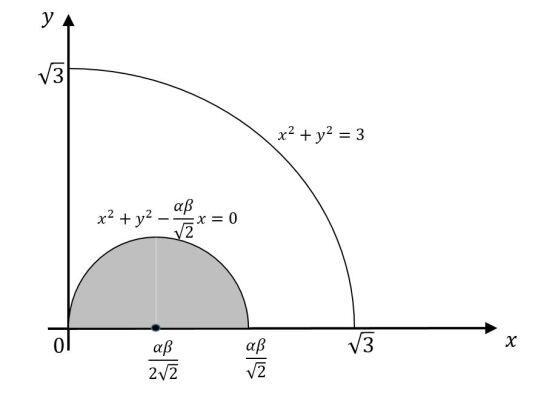
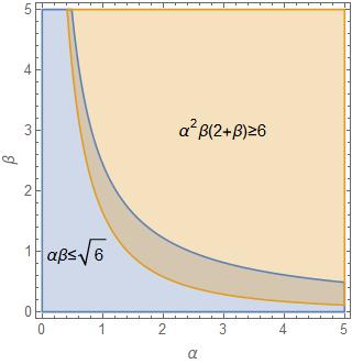
Figure 1: Left : Two curves $x^{2}+y^{2}=3$ and $x^{2}+y^{2}-\frac{\alpha\beta}{\sqrt{2}}x=0$ when $\alpha\beta<\sqrt{6}$. The value of $\frac{d\epsilon}{Hdt}$ is positive in the region $x^{2}+y^{2}-\frac{\alpha\beta}{\sqrt{2}}x<0$ which is colored in grey, while negative in the region between two curves, the overlapping region between $x^{2}+y^{2}<3$ and $x^{2}+y^{2}-\frac{\alpha\beta}{\sqrt{2}}x>0$. Right : Overlapping region between $\alpha\beta\leq\sqrt{6}$ and $\alpha^{2}\beta(2+\beta)\geq 6$, which allows the fixed point value $\epsilon=\frac{3\beta}{2+\beta}$.

When $\alpha\beta<\sqrt{6}$, $\frac{d\epsilon}{Hdt}$ is positive in the region

$$\begin{split}x^{2}+y^{2}-\frac{\alpha\beta}{\sqrt{2}}x<0\end{split}$$ (17)

(colored in grey in the left panel of Fig. 1), the whole of which is inside the region $x^{2}+y^{2}<3$ (or equivalently, $V>0$) as depicted in the left panel of Fig. 1. Since $\frac{d\epsilon}{Hdt}$ is negative in the overlapping region between $x^{2}+y^{2}<3$ and $x^{2}+y^{2}-\frac{\alpha\beta}{\sqrt{2}}x>0$, the point $(x,y)$ on the curve $x^{2}+y^{2}=3$, at which $\frac{d\epsilon}{Hdt}=0$ and $\epsilon=3$, corresponds to the unstable fixed point. Meanwhile, as can be found in the discussion on Case 1 in Sec. 2, the values of $\epsilon$ as well as $(x,y)$ at the fixed points satisfying $x^{2}+y^{2}-\frac{\alpha\beta}{\sqrt{2}}x=0$ are given as follows:

$$\begin{split}\epsilon=\frac{3\beta}{2+\beta}\quad&{\rm at}\quad x=\frac{3\sqrt{2}}{\alpha(2+\beta)},\quad y=\frac{\sqrt{3(\alpha^{2}\beta(2+\beta)-6)}}{\alpha(2+\beta)},\\ \epsilon=\frac{(\alpha\beta)^{2}}{2}\quad&{\rm at}\quad x=\frac{\alpha\beta}{\sqrt{2}},\quad y=0.\end{split}$$ (18)

It is obvious from (12) that the values of $x$ and $y$ at the fixed point are physically sensible provided $\epsilon\leq\frac{(\alpha\beta)^{2}}{2}$, which can be found from the fact that the value of $x$ on the curve $x^{2}+y^{2}-\frac{\alpha\beta}{\sqrt{2}}x=0$ is smaller than $\frac{\alpha\beta}{\sqrt{2}}$ where $\epsilon=\frac{(\alpha\beta)^{2}}{2}$ (see Fig. 1). In particular, for $(x,y)$ corresponding to the fixed point value $\epsilon=\frac{3\beta}{2+\beta}$ to exist, $\alpha$ and $\beta$ must satisfy $\alpha^{2}\beta(2+\beta)\geq 6$. The values of $\alpha$ and $\beta$ belonging to the overlapping region between $\alpha\beta<\sqrt{6}$ and $\alpha^{2}\beta(2+\beta)\geq 6$ are shown in the right panel of Fig. 1. For the axio-dilaton in Type IIB string compactification, $(\alpha,\beta)=(\sqrt{2},1)$, hence $\alpha\beta=\sqrt{2}<\sqrt{6}$ and $\alpha^{2}\beta(2+\beta)=6$. In this case, two fixed points coincide, i.e.,

$$\begin{split}\epsilon=\frac{3\beta}{2+\beta}=\frac{(\alpha\beta)^{2}}{2}=1,\end{split}$$ (19)

at $(x,y)=(1,0)$.

Meanwhile, when $\alpha\beta=\sqrt{6}$, two curves $x^{2}+y^{2}=3$ and $x^{2}+y^{2}-\frac{\alpha\beta}{\sqrt{2}}x=0$ intersect at $(x,y)=(\sqrt{3},0)$ giving $\epsilon=3$, which corresponds to Case 3. Moreover, the point $(x,y)$ satisfying $\epsilon=\frac{\alpha\beta}{\sqrt{2}}x$ except for $(\sqrt{3},0)$ corresponds to Case 1, where the fixed point value is given by the first line in (18). An example for this case is the volume modulus in Type IIB string compactification : since $(\alpha,\beta)=(\sqrt{\frac{2}{3}},3)$, we can find two fixed points $\epsilon=3$ at $(x,y)=(\sqrt{3},0)$ and $\epsilon=\frac{9}{5}$ at $(x,y)=(\frac{3\sqrt{3}}{5},\frac{3\sqrt{2}}{5})$.

Now, we investigate the stability of the fixed points we found above. For the fixed point to be stable, the point $(x,y)$ with $\epsilon$ smaller (larger) than the fixed point value (which will be denoted by $\epsilon_{0}$) in the region $\frac{d\epsilon}{Hdt}>0$ ($\frac{d\epsilon}{Hdt}<0$) must evolve into the fixed point. To see this, we consider the values of $x$ and $y$ slightly deviate from the fixed point values and see their time variations $\frac{dx}{Hdt}$ and $\frac{dy}{Hdt}$.

3.1.1 Case 1 with $\epsilon_{0}=\frac{3\beta}{2+\beta}$

For the fixed point corresponding to $\epsilon_{0}=\frac{3\beta}{2+\beta}$ (the first case in (18)), the small deviations around the fixed point

$$\begin{split}&x=\frac{3\sqrt{2}}{\alpha(2+\beta)}+\delta x\equiv x_{0}+\delta x\\ &y=\frac{\sqrt{3(\alpha^{2}\beta(2+\beta)-6)}}{\alpha(2+\beta)}+\delta y\equiv y_{0}+\delta y\end{split}$$ (20)

give

$$\begin{split}&\frac{dx}{Hdt}=-\frac{6(\alpha^{2}(\beta^{2}+3\beta+2)-6)}{\alpha^{2}(2+\beta)^{2}}\delta x-\frac{\sqrt{6(\alpha^{2}\beta(2+\beta)-6)}(\alpha^{2}(\beta+2)^{2}-6)}{\alpha^{2}(2+\beta)^{2}}\delta y,\\ &\frac{dy}{Hdt}=\frac{\sqrt{6(\alpha^{2}\beta(2+\beta)-6)}(\alpha^{2}(\beta+2)+6)}{\alpha^{2}(2+\beta)^{2}}\delta x+\frac{6(\alpha^{2}\beta(2+\beta)-6)}{\alpha^{2}(2+\beta)^{2}}\delta y.\end{split}$$ (21)

Since $\alpha^{2}\beta(2+\beta)>6$, the coefficients of $\delta x$ and $\delta y$ in $\frac{dx}{Hdt}$ are negative while those in $\frac{dy}{Hdt}$ are positive. Then near the fixed point, the condition $\frac{dx}{Hdt}>0$ ($\frac{dx}{Hdt}<0$) can be written as $\delta y<-k_{x}\delta x$ ($\delta y>-k_{x}\delta x$) where

$$\begin{split}k_{x}=\frac{\sqrt{6}(\alpha^{2}(\beta^{2}+3\beta+2)-6)}{\sqrt{(\alpha^{2}\beta(2+\beta)-6)}(\alpha^{2}(\beta+2)^{2}-6)},\end{split}$$ (22)

while the condition $\frac{dy}{Hdt}>0$ ($\frac{dy}{Hdt}<0$) can be written as $\delta y>-k_{y}\delta x$ ($\delta y<-k_{y}\delta x$) where

$$\begin{split}k_{y}=\frac{\alpha^{2}(\beta+2)+6}{\sqrt{6(\alpha^{2}\beta(2+\beta)-6)}}.\end{split}$$ (23)

Here $k_{x}$ and $k_{y}$ are both positive but do not coincide. In fact, for any positive $\alpha$ and $\beta$ satisfying $\alpha^{2}\beta(2+\beta)-6>0$, $k_{x}$ is always smaller than $k_{y}$. We will compare them with the tangent line of $x^{2}+y^{2}=\epsilon_{0}=$(constant) and that of $x^{2}+y^{2}-\frac{\alpha\beta}{\sqrt{2}}x=0$ at the fixed point, which are given by $\delta y=-c_{0}\delta x$, where

$$\begin{split}c_{0}=\frac{\sqrt{6}}{\sqrt{(\alpha^{2}\beta(2+\beta)-6)}}\end{split}$$ (24)

and $\delta y=-c_{1}\delta x$, where

$$\begin{split}c_{1}=-\frac{\alpha^{2}\beta(2+\beta)-12}{2\sqrt{6}\sqrt{(\alpha^{2}\beta(2+\beta)-6)}}.\end{split}$$ (25)

respectively. We note that whereas $c_{0}$ is positive, $c_{1}$ is positive (negative) if $x_{0}$ is larger (smaller) than $\frac{\alpha\beta}{2\sqrt{2}}$, the $x$ value of the center of the circle $x^{2}+y^{2}-\frac{\alpha\beta}{\sqrt{2}}x=0$, which is obvious from Fig. 1. Moreover, when $c_{1}$ is positive, one immediately finds that $c_{0}>c_{1}$. While $|c_{1}|$ may be larger than $c_{0}$ for a negative $c_{1}$, it is not relevant to our discussion.

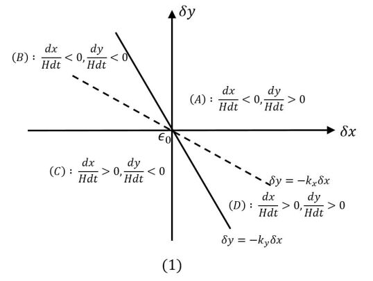
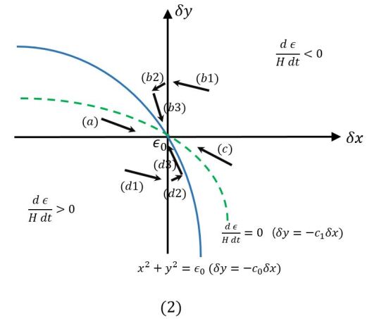
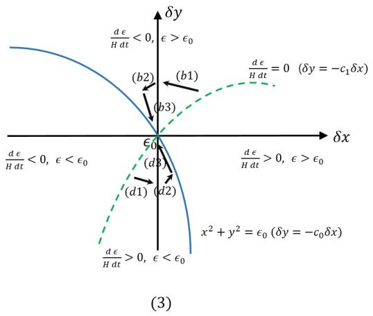
Figure 2: (1) : The regions near the fixed point $\epsilon_{0}$ distinguished by the signs of $\frac{dx}{Hdt}$ and $\frac{dy}{Hdt}$. Here $\frac{dx}{Hdt}=0$ on the black dashed line $\delta y=-k_{x}\delta x$ and $\frac{dy}{Hdt}=0$ on the black line $\delta y=-k_{y}\delta x$. We note that $k_{x}<k_{y}$. (2) : Possible time evolutions of $(x,y)$ when $\alpha^{2}\beta(2+\beta)<12$. The arrows indicate the time evolutions of $(x,y)$ near the fixed point when the fixed point is stable. The blue line and the green dashed line indicate the curves $x^{2}+y^{2}=\epsilon_{0}$ (approximated by $\delta y=-c_{0}\delta x$) and $\frac{d\epsilon}{Hdt}=0$ (or equivalently, $x^{2}+y^{2}-\frac{\alpha\beta}{\sqrt{2}}x=0$ : approximated by $\delta y=-c_{1}\delta x$), respectively. (3) Possible time evolutions of $(x,y)$ when $\alpha^{2}\beta(2+\beta)\geq 12$.

From observations so far, we investigate the stability of the fixed point. Since $k_{x}<k_{y}$, the region around the fixed point can be divided according to the signs of $\frac{dx}{Hdt}$ and $\frac{dy}{Hdt}$ as shown in Fig. 2 (1). We first consider the case $\alpha^{2}\beta(2+\beta)<12$, that is, $x_{0}$ is larger than $\frac{\alpha\beta}{2\sqrt{2}}$. When the point $(x,y)=(x_{0}+\delta x,y_{0}+\delta y)$ satisfies both $\epsilon<\epsilon_{0}$ and $\frac{d\epsilon}{Hdt}>0$, it belongs to the overlapping region between $\delta y<-c_{0}\delta x$ and $\delta y<-c_{1}\delta x$ for sufficiently small values of $\delta x$ and $\delta y$ (see Fig. 2 (2)). If $\delta x<0$ and $\delta y>0$ for $(x,y)$ in this case, the fixed point is stable with respect to the time evolution of $(x,y)$ provided $\frac{dx}{Hdt}>0$ and $\frac{dx}{Hdt}<0$ are satisfied, i.e., $(x,y)$ belongs to the region (C) in Fig. 2 (1) and evolves following the arrow (a) in Fig. 2 (2). Indeed, since $c_{1}<k_{x}$, this condition is trivially fulfilled for any $\alpha$ and $\beta$ satisfying $\alpha^{2}\beta(2+\beta)-6>0$ (otherwise, $y_{0}$ is not well defined : see (18)). Moreover, the relation $c_{1}<k_{x}$ also allows the stability of the fixed point with respect to the evolution of $(x,y)$ with $\delta x>0$ and $\delta y<0$ when it is in the overlapping region between $\delta y>-c_{0}\delta x$ and $\delta y>-c_{1}\delta x$. In this case, $(x,y)$ satisfies $\epsilon>\epsilon_{0}$ and $\frac{d\epsilon}{Hdt}<0$ and its time evolution follows the arrow (c) in Fig. 2 (2). Meanwhile, if $\delta x<0$ and $\delta y<0$, since $\frac{dx}{Hdt}>0$ and $\frac{dy}{Hdt}<0$, $(x,y)$ moves away from the fixed point, following the arrow (d1). However, if $(x,y)$ in this case can evolve into the region $(\frac{dx}{Hdt}>0,\frac{dy}{Hdt}>0)$ (the region (D)) and then into the region $(\frac{dx}{Hdt}<0,\frac{dy}{Hdt}>0)$ (the region (A)) following the arrows (d1)$\to$(d2)$\to$(d3), it can reach the fixed point. Since all these processes take place satisfying $\frac{d\epsilon}{Hdt}>0$ (that is, $\epsilon$ increases in time), $\epsilon$ must be always smaller than $\epsilon_{0}$, which imposes the condition $c_{0}<k_{x}$. But this is not satisfied for any $\alpha$ and $\beta$ satisfying $\alpha^{2}\beta(2+\beta)-6>0$ so the fixed point is not stable under the evolution of $(x,y)$ in the region $\delta y<0$ and $\epsilon<\epsilon_{0}$. The same argument is used to show that the fixed point is not stable for $(x,y)$ satisfying $\delta y>0$ and $\epsilon>\epsilon_{0}$ : the arrow (b3) is not allowed. In summary, when $\alpha^{2}\beta(2+\beta)<12$, the fixed point is stable with respect to the time evolution of $(x,y)$ only if

$$\begin{split}&\delta x<0,~{}\delta y>0\quad{\rm for}~{}\epsilon<\epsilon_{0}~{}{\rm and}~{}\frac{d\epsilon}{Hdt}>0,\\ &\delta x>0,~{}\delta y<0\quad{\rm for}~{}\epsilon>\epsilon_{0}~{}{\rm and}~{}\frac{d\epsilon}{Hdt}<0.\end{split}$$ (26)

Indeed, the volume modulus in Type IIB string compactification corresponds to this case : from $(\alpha,\beta)=(\sqrt{\frac{2}{3}},3)$ we find that $\alpha^{2}\beta(2+\beta)=10$ is larger than $6$ but smaller than $12$ and the slopes appearing in our discussion are given by $c_{0}=\sqrt{\frac{3}{2}}$, $c_{1}=\frac{1}{2\sqrt{6}}$, $k_{x}=\frac{11}{16}\sqrt{\frac{3}{2}}$, and $k_{y}=\frac{7}{3}\sqrt{\frac{2}{3}}$, respectively. Therefore, the fixed point $\epsilon=\frac{9}{5}$ at $(x,y)=(\frac{3\sqrt{3}}{5},\frac{3\sqrt{2}}{5})$ is partially stable.

The stability of the fixed point in the case of $\alpha^{2}\beta(2+\beta)\geq 12$, i.e., $x_{0}\leq\frac{\alpha\beta}{2\sqrt{2}}$, can be tested in the same manner. When the point $(x,y)$ is located in the region $\frac{d\epsilon}{Hdt}<0$ and $\epsilon>\epsilon_{0}$, it can reach the fixed point provided it evolves into the region $(\frac{dx}{Hdt}>0,\frac{dy}{Hdt}<0)$ (the region (C)), where the time evolution of $(x,y)$ follows an arrow (b3) in Fig. 2 (3). This requires $c_{0}<k_{x}$ which however is not satisfied for any $\alpha$ and $\beta$ satisfying $\alpha^{2}\beta(2+\beta)-6>0$. Consideration of the evolution of $(x,y)$ in the region $\frac{d\epsilon}{Hdt}>0$ and $\epsilon<\epsilon_{0}$ also gives the same conclusion. Thus, the fixed point in the region $\alpha^{2}\beta(2+\beta)\geq 12$ is not stable.

3.1.2 Case 1 with $\epsilon_{0}=\frac{(\alpha\beta)^{2}}{2}$, Case 3

We now consider the fixed point corresponding to $\epsilon_{0}=\frac{(\alpha\beta)^{2}}{2}$, the perturbation around which is given by

$$\begin{split}x=\frac{\alpha\beta}{\sqrt{2}}+\delta x,\quad y=\delta y.\end{split}$$ (27)

In this case, in the region $\delta x<0$ ($\delta x>0$), the value of $\epsilon$ is smaller (larger) than the fixed point value and $\frac{d\epsilon}{Hdt}>0$ ($\frac{d\epsilon}{Hdt}<0$) is satisfied. The time variations of $x$ and $y$ reads

$$\begin{split}&\frac{dx}{Hdt}=-\Big{(}3-\frac{(\alpha\beta)^{2}}{2}\Big{)}\delta x,\\ &\frac{dy}{Hdt}=\frac{1}{2}(\alpha^{2}\beta(\beta+2)-6)\delta y.\end{split}$$ (28)

Since the coefficient of $\delta x$ in $\frac{dx}{Hdt}$ is negative for $\alpha\beta<\sqrt{6}$, the fixed point is stable provided $\alpha^{2}\beta(\beta+2)<6$ such that the coefficient of $\delta y$ in $\frac{dy}{Hdt}$ is also negative. Meanwhile, when $\alpha\beta=\sqrt{6}$, which corresponds to Case 3, the coefficient of $\delta x$ in $\frac{dx}{Hdt}$ vanishes whereas the coefficient of $\delta y$ in $\frac{dy}{Hdt}$ is given by the positive number $\sqrt{6}\alpha$. This shows that the value of $y$ tends to move away from the fixed point value hence the fixed point in this case is not stable as well. Applying this to Type IIB string compactification, one finds that the fixed point of the axio-dilaton, $(x,y)=(1,0)$ giving $\epsilon=1$ and that of the volume modulus, $(x,y)=(\sqrt{3},0)$ giving $\epsilon=3$ are unstable.

3.2 $\alpha\beta>\sqrt{6}$

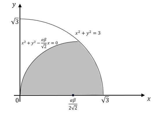
Figure 3: Two curves $x^{2}+y^{2}=3$ and $x^{2}+y^{2}-\frac{\alpha\beta}{\sqrt{2}}x=0$ when $\alpha\beta>\sqrt{6}$. The value of $\frac{d\epsilon}{Hdt}$ is positive in the overlapping region between $x^{2}+y^{2}<3$ and $x^{2}+y^{2}-\frac{\alpha\beta}{\sqrt{2}}x<0$, which is colored in grey, while negative in its complement region, i.e., the overlapping region between $x^{2}+y^{2}<3$ and $x^{2}+y^{2}-\frac{\alpha\beta}{\sqrt{2}}x>0$.

When $\alpha\beta>\sqrt{6}$, only a part of the region $x^{2}+y^{2}-\frac{\alpha\beta}{\sqrt{2}}x<0$ overlaps with $x^{2}+y^{2}\leq 3$, and the values of $(x,y)$ belonging to this overlapping region (colored in grey in Fig. 3) satisfy $\frac{d\epsilon}{Hdt}>0$. Then we expect that the stable fixed point belongs to the boundary of the region $\frac{d\epsilon}{Hdt}>0$ consisting of a part of the curve $x^{2}+y^{2}-\frac{\alpha\beta}{\sqrt{2}}x=0$ and that of the curve $x^{2}+y^{2}=3$. The intersection point between two curves corresponds to Case 3, at which $\epsilon=3$ and a pair of values $(x,y)$ is given by (15), but as we have seen, both $\frac{dx}{Hdt}$ and $\frac{dy}{Hdt}$ do not vanish there. Indeed, since $\frac{dx}{Hdt}<0$ and $\frac{dy}{Hdt}>0$ at the intersection (see (16)), the point $(x,y)$ in this case eventually evolves into the part of the curve $x^{2}+y^{2}=3$ which does not belong to the boundary of the region $\frac{d\epsilon}{Hdt}>0$. In fact, once $\epsilon$ becomes $3$, $(x,y)$ keeps rotating around the circle $x^{2}+y^{2}=3$, even allowing the negative values of $x$ or $y$ (that is, the saxion may climb up the potential). The part of the curve $x^{2}+y^{2}=3$ belonging to the boundary of the region $\frac{d\epsilon}{Hdt}>0$ corresponds to Case 2, in which the value $\epsilon=3$ does not change in time despite the time evolution of $(x,y)$. As can be found in (14), $\frac{dx}{Hdt}<0$ and $\frac{dy}{Hdt}>0$ in this case, which means that the point $(x,y)$ satisfying $\epsilon=3$ keeps rotating on the curve $x^{2}+y^{2}=3$ as mentioned above. Meanwhile, the fixed point on a part of the curve $x^{2}+y^{2}-\frac{\alpha\beta}{\sqrt{2}}x=0$ belonging to the boundary of the region $\frac{d\epsilon}{Hdt}>0$ corresponds to Case 1. In this case, $\epsilon=\frac{3\beta}{2+\beta}$ and the values of $x$ and $y$ are given by (12). While (12) requires $(\alpha\beta)^{2}\geq 2\epsilon$ (or equivalently, $\alpha^{2}\beta(2+\beta)>6$), this condition is trivially fulfilled when $\alpha\beta>\sqrt{6}$ but $\epsilon<3$. The argument on the stability under the perturbation is the same as that in the case of $\alpha\beta\leq\sqrt{6}$, so we conclude that the fixed point is partially stable provided $\alpha^{2}\beta(2+\beta)<12$. Another fixed point corresponding to Case 1, $\epsilon=\frac{(\alpha\beta)^{2}}{2}$ is not allowed since it contradicts to the positivity of the potential ($\epsilon<3$) when $\alpha\beta>\sqrt{6}$.

4 Fixed point in the multifield model

In the presence of multi-pair of saxions and axions $(u_{i},v_{i})$, the action is given by

$$\begin{split}S=\int d^{4}xa(t)^{3}\Big{(}\sum_{i}\frac{M_{\rm Pl}^{2}}{2\alpha_{i}^{2}}\frac{{\dot{u}_{i}}(t)^{2}+{\dot{v}_{i}}(t)^{2}}{u_{i}(t)^{2}}-V\Big{)},\end{split}$$ (29)

where the tree level potential $V$ does not depend on axions $v_{i}$, from which we obtain the following equations of motion :

$$\begin{split}&3M_{\rm Pl}^{2}H^{2}=\sum_{i}\frac{M_{\rm Pl}^{2}}{2\alpha_{i}^{2}}\frac{{\dot{u}_{i}}^{2}+{\dot{v}_{i}}^{2}}{u_{i}^{2}}+V,\\ &3M_{\rm Pl}^{2}H^{2}+2M_{\rm Pl}^{2}\dot{H}=-\sum_{i}\frac{M_{\rm Pl}^{2}}{2\alpha_{i}^{2}}\frac{{\dot{u}_{i}}^{2}+{\dot{v}_{i}}^{2}}{u_{i}^{2}}+V,\\ &\ddot{u_{i}}+3H\dot{u_{i}}-\frac{{\dot{u}_{i}}^{2}}{u_{i}}+\frac{{\dot{v}_{i}}^{2}}{u_{i}}+\frac{\alpha_{i}^{2}}{M_{\rm Pl}^{2}}u_{i}^{2}\frac{\partial V}{\partial u_{i}}=0,\\ &\ddot{v_{i}}+3H\dot{v_{i}}-2\frac{{\dot{u}_{i}}{\dot{v}_{i}}}{u_{i}}=0.\end{split}$$ (30)

We are interested in the volume modulus and the axio-dilaton in Type IIB string compactification which couple to the potential universally (that is, every F-term potential term depends on them in the same way), such that the potential satisfies $u_{i}\frac{\partial V}{\partial u_{i}}=-\beta_{i}V$. Then in terms of

$$\begin{split}x_{i}=\frac{1}{\sqrt{2}\alpha_{i}}\frac{{\dot{u}_{i}}}{Hu_{i}},\quad\quad y_{i}=\frac{1}{\sqrt{2}\alpha_{i}}\frac{{\dot{v}_{i}}}{Hu_{i}},\end{split}$$ (31)

the relations

$$\begin{split}&\epsilon=\sum_{i}(x_{i}^{2}+y_{i}^{2}),\\ &\frac{V}{M_{\rm Pl}^{2}H^{2}}=3-\epsilon,\\ &\frac{\ddot{u}}{H^{2}u_{i}}=-3\sqrt{2}\alpha_{i}x_{i}+2\alpha_{i}^{2}x_{i}^{2}-2\alpha_{i}^{2}y_{i}^{2}+\alpha_{i}^{2}\beta_{i}(3-\epsilon),\\ &\frac{\ddot{v}}{H^{2}u_{i}}=-3\sqrt{2}\alpha_{i}y_{i}+4\alpha_{i}^{2}x_{i}y_{i}.\end{split}$$ (32)

are obeyed, then we obtain

$$\begin{split}&\frac{dx_{i}}{Hdt}=\frac{1}{\sqrt{2}\alpha_{i}}\Big{[}\frac{\ddot{u}_{i}}{H^{2}u_{i}}-\Big{(}\frac{\dot{u}_{i}}{Hu_{i}}\Big{)}^{2}+\epsilon\frac{\dot{u}_{i}}{Hu_{i}}\Big{]}=(\epsilon-3)\Big{(}x_{i}-\frac{\alpha_{i}\beta_{i}}{\sqrt{2}}\Big{)}-\sqrt{2}\alpha_{i}y_{i}^{2},\\ &\frac{dy_{i}}{Hdt}=\frac{1}{\sqrt{2}\alpha_{i}}\Big{[}\frac{\ddot{v}_{i}}{H^{2}u_{i}}-\frac{\dot{u}_{i}}{Hu_{i}}\frac{\dot{v}_{i}}{Hu_{i}}+\epsilon\frac{\dot{v}_{i}}{Hu_{i}}\Big{]}=(\epsilon-3)y_{i}+\sqrt{2}\alpha_{i}x_{i}y_{i}.\end{split}$$ (33)

At the fixed point, the value of $\epsilon$ does not vary in time, i.e.,

$$\begin{split}\frac{d\epsilon}{Hdt}=2(\epsilon-3)\Big{(}\epsilon-\sum_{i}\frac{\alpha_{i}\beta_{i}}{\sqrt{2}}x_{i}\Big{)}=0.\end{split}$$ (34)

We first consider the case $\epsilon=\sum_{i}\frac{\alpha_{i}\beta_{i}}{\sqrt{2}}x_{i}$, which corresponds to the generalization of Case 1 and 3 in Sec. 2. At first glance, the condition that the combination $\sum_{i}\frac{\alpha_{i}\beta_{i}}{\sqrt{2}}x_{i}$ which is identified with $\epsilon$ is a constant in time is less restrictive than the single field case ($\frac{dx_{i}}{Hdt}=\frac{dy_{i}}{Hdt}=0$), but it is not always the case. To see this, we consider the simplest case in which two saxion-axion pairs roll down the potential, i.e., the index $i$ runs from $1$ to $2$. Since the combination $\sum_{i}\frac{\alpha_{i}\beta_{i}}{\sqrt{2}}x_{i}$ is a constant in time, we obtain another condition,

$$\begin{split}\frac{d}{Hdt}\sum_{i}\frac{\alpha_{i}\beta_{i}}{\sqrt{2}}x_{i}=(\epsilon-3)\Big{(}\epsilon-\sum_{i}\frac{(\alpha_{i}\beta_{i})^{2}}{2}\Big{)}-\sum_{i}\alpha_{i}^{2}\beta_{i}y_{i}^{2}=0,\end{split}$$ (35)

or equivalently, the combination $\sum_{i}\alpha_{i}^{2}\beta_{i}y_{i}^{2}$ is also a constant in time. Then from

$$\begin{split}\frac{d}{Hdt}\sum_{i}\alpha_{i}^{2}\beta_{i}y_{i}^{2}=2(\epsilon-3)^{2}\Big{(}\epsilon-\sum_{i}\frac{(\alpha_{i}\beta_{i})^{2}}{2}\Big{)}+2\sqrt{2}\sum_{i}\alpha_{i}^{3}\beta_{i}x_{i}y_{i}^{2}=0,\end{split}$$ (36)

we obtain the new condition that the combination $\sum_{i}\alpha_{i}^{3}\beta_{i}x_{i}y_{i}^{2}$ is a constant in time :

$$\begin{split}\frac{d}{Hdt}\sum_{i}\alpha_{i}^{3}\beta_{i}x_{i}y_{i}^{2}=&-\frac{3}{\sqrt{2}}(\epsilon-3)^{3}\Big{(}\epsilon-\sum_{i}\frac{(\alpha_{i}\beta_{i})^{2}}{2}\Big{)}-(\epsilon-3)\sum_{i}\frac{\alpha_{i}^{4}\beta_{i}^{2}}{\sqrt{2}}y_{i}^{2}\\ &-\sqrt{2}\sum_{i}\alpha_{i}^{4}\beta_{i}(y_{i}^{4}-2x_{i}^{2}y_{i}^{2})\\ =&0.\end{split}$$ (37)

Then conditions (35), (36), and (37), together with $\sum_{i}(x_{i}^{2}+y_{i}^{2})=\epsilon$ and $\sum_{i}\frac{\alpha_{i}\beta_{i}}{\sqrt{2}}x_{i}=\epsilon$ uniquely determine the values of $(x_{1},x_{2},y_{i},y_{2},\epsilon)$. In particular, each of $x_{i}$ and $y_{i}$ is a constant in time so we do not need to take further time derivatives to obtain additional conditions. For example, in Type IIB string compactification, the values of $(\alpha_{i},\beta_{i})$ for the volume modulus and the axio-dilaton are given by $(\sqrt{\frac{2}{3}},3)$ and $(\sqrt{2},1)$, respectively, from which five conditions read

$$\begin{split}&(1)\quad x_{1}^{2}+y_{1}^{2}+x_{2}^{2}+y_{2}^{2}=\epsilon,\\ &(2)\quad\sqrt{3}x_{1}+x_{2}=\epsilon,\\ &(3)\quad(\epsilon-3)(\epsilon-4)=2(y_{1}^{2}+y_{2}^{2}),\\ &(4)\quad-\frac{1}{4}(\epsilon-3)^{2}(\epsilon-4)=\frac{1}{\sqrt{3}}x_{1}y_{1}^{2}+x_{2}y_{2}^{2},\\ &(5)\quad-\frac{1}{\sqrt{2}}(\epsilon-3)^{2}(\epsilon-4)-\frac{4}{\sqrt{2}}(\epsilon-3)(y_{1}^{2}+y_{2}^{2})+4\sqrt{2}(\epsilon-3)\Big{(}\frac{1}{\sqrt{3}}x_{1}y_{1}^{2}+x_{2}y_{2}^{2}\Big{)}\\ &\quad\quad\quad-4\sqrt{2}\Big{(}\frac{1}{3}(y_{1}^{4}-2x_{1}^{2}y_{1}^{2})+(y_{2}^{4}-2x_{2}^{2}y_{2}^{2})=0.\end{split}$$ (38)

Solving these conditions, we obtain following values of $(x_{1},x_{2},y_{i},y_{2},\epsilon)$ :

$$\begin{split}&({\rm A})\quad\epsilon=2\quad{\rm at}\quad x_{1}=\frac{\sqrt{3}}{2},\quad y_{1}=\frac{\sqrt{3}}{2}\quad x_{1}=\frac{1}{2},\quad y_{2}=\frac{1}{2},\\ &({\rm B})\quad\epsilon=\frac{11}{5}\quad{\rm at}\quad x_{1}=\frac{2\sqrt{3}}{5},\quad y_{1}=\frac{3\sqrt{2}}{5}\quad x_{1}=1,\quad y_{2}=0,\end{split}$$ (39)

which correspond to Case 1, and

$$\begin{split}&({\rm C})\quad\epsilon=3\quad{\rm at}\quad x_{1}=\frac{\sqrt{3}}{2},\quad y_{1}=0\quad x_{1}=\frac{3}{2},\quad y_{2}=0,\\ &({\rm D})\quad\epsilon=3\quad{\rm at}\quad x_{1}=\sqrt{3},\quad y_{1}=0\quad x_{1}=0,\quad y_{2}=0,\end{split}$$ (40)

which correspond to Case 3. To see the stability of the fixed points, we consider the variations $\frac{dx_{i}}{Hdt}$ and $\frac{dy_{i}}{Hdt}$ at linear order in $(\delta x_{i},\delta y_{i})$ given by

$$\begin{split}({\rm A})\quad:\quad&\frac{dx_{1}}{Hdt}=-\frac{5}{2}\delta x_{1}-\frac{\sqrt{3}}{2}\delta x_{2}-\frac{7}{2}\delta y_{1}-\frac{\sqrt{3}}{2}\delta y_{2},\\ &\frac{dy_{1}}{Hdt}=\frac{5}{2}\delta x_{1}+\frac{\sqrt{3}}{2}\delta x_{2}+\frac{3}{2}\delta y_{1}+\frac{\sqrt{3}}{2}\delta y_{2},\\ &\frac{dx_{2}}{Hdt}=-\frac{\sqrt{3}}{2}\delta x_{1}-\frac{3}{2}\delta x_{2}-\frac{\sqrt{3}}{2}\delta y_{1}-\frac{5}{2}\delta y_{2},\\ &\frac{dy_{2}}{Hdt}=\frac{\sqrt{3}}{2}\delta x_{1}+\frac{3}{2}\delta x_{2}+\frac{\sqrt{3}}{2}\delta y_{1}+\frac{1}{2}\delta y_{2},\end{split}$$ (41)

$$\begin{split}({\rm B})\quad:\quad&\frac{dx_{1}}{Hdt}=-\frac{56}{25}\delta x_{1}-\frac{6\sqrt{3}}{5}\delta x_{2}-\frac{38\sqrt{6}}{25}\delta y_{1},\\ &\frac{dy_{1}}{Hdt}=\frac{22\sqrt{6}}{25}\delta x_{1}+\frac{6\sqrt{2}}{5}\delta x_{2}+\frac{36}{25}\delta y_{1},\\ &\frac{dx_{2}}{Hdt}=-\frac{4}{5}\delta x_{2},\quad\frac{dy_{2}}{Hdt}=\frac{6}{5}\delta y_{2},\end{split}$$ (42)

$$\begin{split}({\rm C})\quad:\quad&\frac{dx_{1}}{Hdt}=-\frac{3}{2}\delta x_{1}-\frac{3\sqrt{3}}{2}\delta x_{2},\quad\frac{dy_{1}}{Hdt}=\delta y_{1},\\ &\frac{dx_{2}}{Hdt}=\frac{\sqrt{3}}{2}\delta x_{1}+\frac{3}{2}\delta x_{2},\quad\frac{dy_{2}}{Hdt}=3\delta y_{2},\end{split}$$ (43)

$$\begin{split}({\rm D})\quad:\quad&\frac{dx_{1}}{Hdt}=0,\quad\frac{dy_{1}}{Hdt}=2\delta y_{1},\\ &\frac{dx_{2}}{Hdt}=-2\sqrt{3}\delta x_{1},\quad\frac{dy_{2}}{Hdt}=0.\end{split}$$ (44)

Then we find that for the cases (B), (C), and (D), at least one time variation of $y_{i}$ is given by the form $\frac{dy_{i}}{Hdt}=\gamma\delta y_{i}$ with some positive $\gamma_{i}$, which indicates that the fixed point is not stable with respect to the direction of $y_{i}$. Moreover, for the case (A), which corresponds to Case 1 in Sec. 2 with $\epsilon_{0}=\frac{3\beta}{2+\beta}$, the fixed point is on the meridian of the ellipsoid $\epsilon=\sum_{i}\frac{\alpha_{i}\beta_{i}}{\sqrt{2}}x_{i}$, which is written as $(x_{1}-\frac{\sqrt{3}}{2})^{2}+(x_{2}-\frac{1}{2})^{2}+y_{1}^{2}+y_{2}^{2}=1$. In the language of Case 1 in Sec. 2, the fixed point value of $x$ is not larger than the value of $x$ at the center of the curve $x^{2}+y^{2}-\frac{\alpha\beta}{\sqrt{2}}x=0$. This implies that the direction like the arrow (a) or (c) in Fig. 2 (2) does not exist hence the fixed point is not stable.

Meanwhile, when $\epsilon=3$ but the combination $\sum_{i}\frac{\alpha_{i}\beta_{i}}{\sqrt{2}}x_{i}$ is not necessarily identified with $\epsilon$ (the generalization of Case 2), time variations of $x_{i}$ and $y_{i}$ satisfy

$$\begin{split}\frac{dx_{i}}{Hdt}=-\sqrt{2}\alpha_{i}y_{i}^{2},\quad\frac{dy_{i}}{Hdt}=\sqrt{2}\alpha_{i}x_{i}y_{i}.\end{split}$$ (45)

From this, we immediately find that for each pair of $(u_{i},v_{i})$, the combination $x_{i}^{2}+y_{i}^{2}$ is a constant in time. In this case, even though $x_{i}$ and $y_{i}$ vary in time, so far as they are on the curve $\epsilon=3$ the value of $\epsilon$ does not change in time.

5 Conclusions

We studied the fixed point values of the slow-roll parameter $\epsilon$ and their stability when the axion as well as the saxion moves in the quintessence model. Even though the potential at tree level does not depend on the axion due to the shift symmetry, the axion couples to the saxion as well as the background geometry. As a result, the axion can move as the saxion rolls down the runaway potential. Then the axion kinetic energy contributes to the vacuum energy density and $\epsilon$ in nontrivial ways at the fixed point where the slow-roll approximation does not hold. Even in this case, just like the case in which only the saxion moves, the value of $\epsilon$ is restricted to be smaller than $3$, which is imposed by the positivity of the potential, and its properties at the fixed point depend on $\alpha$ and $\beta$. We also find that the fixed point is in general not stable with respect to the time evolution from all directions in the field space. To see this more concretely, we consider the volume modulus and the axio-dilaton, which are the essential ingredients of the string compactification and couple to the potential universally. When one of them is fixed, there exist some partially stable fixed points and if the value of $\epsilon$ is given by $3$, the largest value imposed by the positivity of the potential, it is not changed even if the values of $x$ and $y$ vary in time. If both of them are allowed to move, we find that the stable fixed point does not exist. Our analysis shows that the addition of the axion in the stringy quintessence model can exhibit different feature from the simplest model in which only the saxion is dynamical.

Acknowledgements

This work is motivated by Filippo Revello’s question about the author’s previous work [32].

References

- [1]
- [2] N. Aghanim et al. [Planck], Astron. Astrophys. 641 (2020), A6 [erratum: Astron. Astrophys. 652 (2021), C4] [arXiv:1807.06209 [astro-ph.CO]].
- [3] S. Kachru, R. Kallosh, A. D. Linde and S. P. Trivedi, Phys. Rev. D 68 (2003), 046005 [arXiv:hep-th/0301240 [hep-th]].
- [4] V. Balasubramanian, P. Berglund, J. P. Conlon and F. Quevedo, JHEP 03 (2005), 007 [arXiv:hep-th/0502058 [hep-th]].
- [5] M. Dine and N. Seiberg, Phys. Lett. B 162 (1985), 299-302
- [6] S. B. Giddings, S. Kachru and J. Polchinski, Phys. Rev. D 66 (2002), 106006 [arXiv:hep-th/0105097 [hep-th]].
- [7] S. Kachru, J. Pearson and H. L. Verlinde, JHEP 06 (2002), 021 [arXiv:hep-th/0112197 [hep-th]].
- [8] S. Hellerman, N. Kaloper and L. Susskind, JHEP 06 (2001), 003 [arXiv:hep-th/0104180 [hep-th]].
- [9] W. Fischler, A. Kashani-Poor, R. McNees and S. Paban, JHEP 07 (2001), 003 [arXiv:hep-th/0104181 [hep-th]].
- [10] N. Kaloper and L. Sorbo, Phys. Rev. D 79 (2009), 043528 [arXiv:0810.5346 [hep-th]].
- [11] M. Cicoli, F. G. Pedro and G. Tasinato, JCAP 07 (2012), 044 [arXiv:1203.6655 [hep-th]].
- [12] P. Agrawal, G. Obied, P. J. Steinhardt and C. Vafa, Phys. Lett. B 784 (2018), 271-276 doi:10.1016/j.physletb.2018.07.040 [arXiv:1806.09718 [hep-th]].
- [13] M. Cicoli, S. De Alwis, A. Maharana, F. Muia and F. Quevedo, Fortsch. Phys. 67 (2019) no.1-2, 1800079 [arXiv:1808.08967 [hep-th]].
- [14] M. C. David Marsh, Phys. Lett. B 789 (2019), 639-642 [arXiv:1809.00726 [hep-th]].
- [15] A. Hebecker, T. Skrzypek and M. Wittner, JHEP 11 (2019), 134 [arXiv:1909.08625 [hep-th]].
- [16] Y. Olguin-Trejo, S. L. Parameswaran, G. Tasinato and I. Zavala, JCAP 01 (2019), 031 [arXiv:1810.08634 [hep-th]].
- [17] B. Valeixo Bento, D. Chakraborty, S. L. Parameswaran and I. Zavala, PoS CORFU2019 (2020), 123 [arXiv:2005.10168 [hep-th]].
- [18] M. Cicoli, F. Cunillera, A. Padilla and F. G. Pedro, Fortsch. Phys. 70 (2022) no.4, 2200009 [arXiv:2112.10779 [hep-th]].
- [19] M. Cicoli, F. Cunillera, A. Padilla and F. G. Pedro, Fortsch. Phys. 70 (2022) no.4, 2200008 [arXiv:2112.10783 [hep-th]].
- [20] M. Brinkmann, M. Cicoli, G. Dibitetto and F. G. Pedro, JHEP 11 (2022), 044 [arXiv:2206.10649 [hep-th]].
- [21] J. P. Conlon and F. Revello, JHEP 11 (2022), 155 [arXiv:2207.00567 [hep-th]].
- [22] T. Rudelius, JHEP 10 (2022), 018 [arXiv:2208.08989 [hep-th]].
- [23] J. Calderón-Infante, I. Ruiz and I. Valenzuela, JHEP 06 (2023), 129 [arXiv:2209.11821 [hep-th]].
- [24] F. Apers, J. P. Conlon, M. Mosny and F. Revello, JHEP 08 (2023), 156 [arXiv:2212.10293 [hep-th]].
- [25] G. Shiu, F. Tonioni and H. V. Tran, Phys. Rev. D 108 (2023) no.6, 063527 [arXiv:2303.03418 [hep-th]].
- [26] G. Shiu, F. Tonioni and H. V. Tran, Phys. Rev. D 108 (2023) no.6, 063528 [arXiv:2306.07327 [hep-th]].
- [27] S. Cremonini, E. Gonzalo, M. Rajaguru, Y. Tang and T. Wrase, JHEP 09 (2023), 075 [arXiv:2306.15714 [hep-th]].
- [28] A. Hebecker, S. Schreyer and G. Venken, JHEP 11 (2023), 173 [arXiv:2306.17213 [hep-th]].
- [29] T. Van Riet, [arXiv:2308.15035 [hep-th]].
- [30] F. Revello, [arXiv:2311.12429 [hep-th]].
- [31] F. Apers, J. P. Conlon, E. J. Copeland, M. Mosny and F. Revello, [arXiv:2401.04064 [hep-th]].
- [32] M. S. Seo, [arXiv:2402.00241 [hep-th]].
- [33] M. S. Seo, Phys. Rev. D 99 (2019) no.10, 106004 [arXiv:1812.07670 [hep-th]].
- [34] S. Mizuno, S. Mukohyama, S. Pi and Y. L. Zhang, JCAP 09 (2019), 072 [arXiv:1905.10950 [hep-th]].