KUNS-2995
Coarse-graining black holes out of equilibrium
with boundary observables on time slice

Abstract

In black hole thermodynamics, defining coarse-grained entropy for dynamical black holes has long been a challenge, and various proposals, such as generalized entropy, have been explored. Guided by the AdS/CFT, we introduce a new definition of coarse-grained entropy for a dynamical black hole in Lorentzian Einstein gravity. On each time slice, this entropy is defined as the horizon area of an auxiliary Euclidean black hole that shares the same mass, (angular) momenta, and asymptotic normalizable matter modes with the original Lorentzian solution. The entropy is shown to satisfy a generalized first law and, through holography, the second law as well. Furthermore, by applying this thermodynamics to several Vaidya models in AdS and flat spacetime, we discover a connection between the second law and the null energy condition.

1 Introduction and summary

Gravity is considered thermodynamic [1]. The zeroth law asserts the existence of intensive variables, which in black hole thermodynamics correspond to quantities constant over the event horizon, such as surface gravity and angular velocity. The first law is one of the key concept, stating the energy conservation among neighboring stationary black holes [2, 3] when the horizon area is viewed as the entropy [4]. Applied to the local Rindler patch, the first law reproduces the Einstein equation, allowing us to regard it as an equation of state [5]. Above all, not only does black hole thermodynamics apply as a formal analogy, but it also has physical reality in the Hawking radiation [6].

Thermodynamics helps us understand spacetime physics, because it gives a macroscopic constraints that the statistical mechanics of a quantum theory of gravity must adhere to. First, the microscopic counting of states in string theory (beginning with [7]) agrees with the horizon area, confirming the importance of exploring fundamental theories through macroscopic observations. Second, given the entropy as a function of sufficient extensive variables, thermodynamics dictates among what states transitions are allowed to happen. This is the role of the second law. Since general relativity itself does not teach what “physical” time evolutions are, energy conditions are necessary for describing “physical” systems. Here, the thermodynamics of spacetime is expected to provide an answer if established.

However, the second law remains under debate. While the Hawking area theorem [8] guarantees that the horizon area does not decrease toward the future, the question as to whether the horizon area can be regarded as the entropy even out of equilibrium is nontrivial. Besides, it is incompatible with the Hawking radiation occurring in the semiclassical regime. An alternative proposal that has been extensively studied is the generalized entropy [9, 10], which is the sum of the entropy of matter outside the horizon on a time slice and the area of the cross section between the horizon and the time slice. Despite numerous attempts, however, a proof of the generalized second law valid in any situation, or an agreement on a suitable definition of the entropy for dynamical black holes has not been achieved (see [11, 12, 13, 14] for review). The second law is one of the primary topics addressed in this paper.

Gravity, on the other hand, is considered holographic. In the classical Einstein gravity, the bulk contribution of the on-shell action vanishes and meaningful values arise from the boundary term, by which we define the energy, (angular) momenta, and other charges. At the same time, the entropy in stationary cases is defined on the causal boundary, the horizon, and interestingly, the first law holds among those boundary values [3].

The holographic nature is a key concept also at the quantum level [17, 18, 19, 20], having provided hints towards quantum gravity. Among those, the AdS/CFT correspondence [21, 22, 23] has attracted significant attention so far. According to the correspondence, the gravitational degrees of freedom are mapped onto the quantum field theory defined on the AdS boundary. Notably, the entanglement entropy is expected to reveal the nature of the dual spacetime [24, 25, 26, 27]. The entanglement entropy of a boundary region is equivalent to the area of an extremal surface in the bulk, and in the semiclassical regime the von Neumann entropy of matter is added to it as quantum corrections [28, 29, 30]; the total entropy takes a form similar to the thermodynamic generalized entropy explained above. This direction recently developed into the Island formula [31, 32, 33, 34, 35] to study the Page curve [36, 37], with applications extending beyond AdS gravity [38].

When applying holography to black hole thermodynamics, particularly concerning the second law, it seems better to introduce coarse-grained entropies. This is because, for instance, the unitarity of the CFT ensures that the fine-grained entropy of a total system state is time-independent, which makes the HRT surface [26] insensitive to any probe sent from the boundary [39]. Within the framework of the AdS/CFT, a coarse-grained entropy associated with the second law in the bulk was first explored in [40], where the one-point entropy was introduced. The relationship with the first law was also investigated in [41]. In [40], the bulk dual of the one-point entropy was first conjectured to be the causal holographic information [42, 43], but unfortunately, counterexamples were identified in [44], leading the authors to conclude that the bulk counterpart seems to be more intricate than initially proposed. Other approaches, as seen in [45, 46, 47, 48], begin with defining their coarse-graining procedures in the bulk. While [45, 47] and [48] employ different ways of coarse-graining, both approaches are associated with the apparent horizon, presenting intriguing implications to gravity and its thermodynamics. However, as noted by the authors, none of those approaches has yet acquired a complete description within the boundary language.

In the same spirit, we propose via the AdS/CFT a new coarse-grained entropy, which is defined both on the boundary and in the bulk. It is valuable to study variety of ways of coarse-graining, as the coarse-grained entropy differs depending on what information one aims to preserve, and different coarse-graining methods will offer different perspectives on gravity. The entropy we propose satisfies a generalized version of the first law, and by the AdS/CFT the second law as well. In addition, it coincides with the Bekenstein-Hawking entropy for stationary solutions.

We begin with the positivity of the relative entropy in the boundary quantum theory. Let $\rho_{1}$ and $\rho_{2}$ be normalized density operators, then the relative entropy is defined as

$$S(\rho_{1}||\rho_{2}):=\mathrm{Tr}(\rho_{1}\ln\rho_{1}-\rho_{1}\ln\rho_{2}),$$ (1.1)

which is always non-negative. Suppose the initial state is a steady state $\rho_{0}$, which evolves to $\rho_{t}$ with a time-dependent Hamiltonian. The time-dependence is triggered by sources coupling to composite operators. On the other hand, we prepare a reference state $\rho_{\mathrm{ref},t}$ sharing with $\rho_{t}$ the same expectation values of composite operators $\{O_{I}\}$ of our interest: $\mathrm{Tr}(\rho_{\mathrm{ref},t}O_{I})=\mathrm{Tr}(\rho_{t}O_{I})$. At $t=0$ we set the reference state as $\rho_{\mathrm{ref},0}=\rho_{0}$. Then, we define our coarse-grained entropy by $S_{t}:=-\mathrm{Tr}(\rho_{\mathrm{ref},t}\ln\rho_{\mathrm{ref},t})$, and will show that $S_{t}\geq S_{0}$ holds for any $t$, based on the positivity $S(\rho_{t}||\rho_{\mathrm{ref},t})\geq 0$.

This coarse-grained entropy is in the bulk equivalent to the horizon area of an auxiliary Euclidean spacetime realized as the dominant saddle point of the gravitational path integral dual to $\rho_{\mathrm{ref},t}$. In the bulk language, $\mathrm{Tr}(\rho_{\mathrm{ref},t}O_{I})=\mathrm{Tr}(\rho_{t}O_{I})$ means that the Euclidean solution shares the same asymptotic normalizable modes with the original Lorentzian time slice. Besides, the second law $S_{t}\geq S_{0}$ means that the horizon area of the Euclidean black hole we refer to at $t$ is always greater than or equal to the horizon area of the initial black hole. This is the second law in this paper. As explained below, this is not an assertion of monotonically increasing area as in Hawking’s area law. After obtaining the gravitational description, we will also derive the first law, which, in addition to the usual terms, contains contributions from the asymptotic matter modes.

We will also check the two laws explicitly in several null-ray collapse models and find that our second law implies the null energy condition — derived by the AdS/CFT, this can be viewed as a consequence of quantum gravity. The gravitational description we finally obtain can formally be applied to non-AdS spacetimes. To test its applicability, an asymptotically flat collapse is chosen as one of the examples, and the two laws actually hold in this example.

It is worth mentioning that the second law in this paper, though not monotonic, is compatible with the expressions of the second law in the context of non-equilibrium thermodynamics. The second law in thermodynamics serves as the criterion for possible transitions between steady states. In non-equilibrium thermodynamics, the second law is generalized to the statement that the entropy production never becomes negative. When the total system is deterministic, the second law follows from the result of [53, 54], where the initial state is prepared as a product state of the system and bath, with the bath in equilibrium. Since the initial state is prepared specially, the monotonicity is not guaranteed. The second law remains monotonic, for example, when the system is Malkovian [55, 56], as a Malkovian system does not care about its history, making the initial state not special anymore. It may not be obvious whether the monotonicity holds for dynamical gravitational systems as well. The quantum versions of the second law without the monotonicity were also shown via the relative entropy in [57, 58] (see [59] for review). The present work is inspired by those inequalities in quantum theory.

The organization of this paper is as follows. In section 2, the second law is derived in the QFT. In section 3, we rewrite it in the bulk Einstein gravity, and also derive the (generalized) first law. In section 4, the derived thermodynamic laws are applied to Vaidya-type models, indicating that thermodynamics constraints gravity.

Summary of the results

Here, the main results in the gravity side is roughly overviewed. Let $M$ be a $(d+1)$-dimensional Lorentzian manifold with timelike boundary $\partial M$. The theory is supposed to be the Einstein theory with matter fields, whose action is denoted as $I_{\mathrm{grav}}$ (see (3.1)). Gauge fields like Maxwell field can be included.

We suppose that a stationary configuration is realized on the initial time slice. This is prepared by analytically continuing a Euclidean solution (figure 3). To define a coarse-grained entropy at time $t>0$, we need to specify a set of fields to be respected, whose values on $\partial M$ we write as $\{w^{I}_{t}(\theta)\}$. Here, $I$ is the label of fields, and the boundary coordinate is written as $z=(t,\theta^{A})$ with $A=1,\cdots,d-1$. The induced metric on $\partial M$ is assumed static, while each $w^{I}_{t}(\theta)$ can depend on time. The normalizable mode conjugate to $w^{I}_{t}(\theta)$ is defined to be

$$\pi_{I,t}(\theta):=\frac{\delta}{\delta w^{I}_{t}(\theta)}\left(\left.I_{\mathrm{grav}}\right|_{\mathrm{on-shell}}[w]\right).$$ (1.2)

We write the mass and the (angular) momenta in $\theta^{A}$-direction as $h_{t}$ and $p_{A,t}$, both of which are defined by the Brown-York tensor (3.8). Note that $\pi_{I,t}(\theta)$ is a local quantity, dependent on the spatial coordinates $\theta^{A}$, while $h_{t}$ and $p_{A,t}$ are independent of $\theta^{A}$.

Our coarse-grained entropy $S_{t}$ is defined by the following procedure. On each time slice, we find the auxiliary Euclidean solution which dominates the gravitational path integral, while respecting $h_{t}$, $p_{A,t}$ and $\pi_{I,t}$ as its mass, (angular) momenta, and asymptotic modes. We assume that this Euclidean solution is realized stationary, independent of the imaginary time. Then, $S_{t}$ is defined to be the horizon area, the area of the cigar tip in figure 4. Since the initial configuration of $M$ is stationary, $S_{0}$ is exactly the Bekenstein-Hawking entropy of the initial black hole.

The main claims of this paper are as follows. First, $\dot{S}_{t}$ (the dot means the time-derivative) is given by the first law, with additional contributions consisting of $\{w^{I}\}$ and $\{\pi_{I}\}$. Second, $S_{t}$ satisfies the second law, $S_{t}\geq S_{0}$. While the first law is derived within the Einstein gravity, the second law is derived via the holographic dictionary. Nevertheless, we conjecture that it must hold also in generic cases under the setup mentioned in the beginning (see section 3.5.1 and 4.3).

2 Coarse-grained state in QFT

In this section, we first introduce the reference state $\rho_{\mathrm{ref},t}$, a coarse-grained state to be compared with the original state at time $t$ through the relative entropy. The second law is derived from the positivity of the relative entropy. After that, in preparation for section 3, we move on to the path integral representation.

2.1 Coarse-grained state and second law

2.1.1 The simplest case

Let us grasp the essence with a warm-up example. We consider a generic quantum theory. The initial state at $t=0$ is supposed to be

$$\rho_{0}=\frac{e^{-\beta H(0)}}{Z_{0}(\beta)},\qquad Z_{0}(\beta):=\mathrm{Tr}e^{-\beta H(0)},$$ (2.1)

where $H(0)$ is the Hamiltonian at $t=0$ and $\beta_{0}$ is an arbitrary inverse temperature. The system evolves with a time-dependent Hamiltonian $H(t)$ as

$$\rho_{t}=U(t)\rho_{0}U(t)^{-1},\qquad U(t):=\mathrm{T}\exp\left(-i\int_{0}^{t}\mathrm{d}s\,H(s)\right).$$ (2.2)

We choose the following as the reference state:

$$\rho_{\mathrm{ref},t}=\frac{e^{-\beta^{\prime}H(t)}}{Z_{t}(\beta^{\prime})},\qquad Z_{t}(\beta^{\prime}):=\mathrm{Tr}e^{-\beta^{\prime}H(t)},$$ (2.3)

with $\beta^{\prime}$ being any positive parameter.

In this setup, we compute the relative entropy $S(\rho_{t}||\rho_{\mathrm{ref},t})$ defined in (1.1). First, since the evolution is unitary, we have

$$\mathrm{Tr}(\rho_{t}\ln\rho_{t})=\mathrm{Tr}(\rho_{0}\ln\rho_{0})=-\ln Z_{0}(\beta)-\beta\mathrm{Tr}\left(\rho_{0}H(0)\right).$$ (2.4)

The remaining piece in (1.1) is readily

$$\mathrm{Tr}(\rho_{t}\ln\rho_{\mathrm{ref},t})=-\ln Z_{t}(\beta^{\prime})-\beta^{\prime}\mathrm{Tr}\left(\rho_{t}H(t)\right).$$ (2.5)

The inequality $S(\rho_{t}||\rho_{\mathrm{ref},t})\geq 0$ reads

$$-\mathrm{Tr}(\rho_{t}\ln\rho_{\mathrm{ref},t})=\beta^{\prime}\mathrm{Tr}\left(\rho_{t}H(t)\right)+\ln Z_{t}(\beta^{\prime})\geq\beta\mathrm{Tr}\left(\rho_{0}H(0)\right)+\ln Z_{0}(\beta).$$ (2.6)

When $\beta^{\prime}$ is set to be $\beta$, the inequality gives [57]

$$\mathrm{Tr}\left(\rho_{t}H(t)\right)-\mathrm{Tr}\left(\rho_{0}H(0)\right)\geq[-\beta^{-1}\ln Z_{t}(\beta)]-[-\beta^{-1}\ln Z_{0}(\beta)].$$ (2.7)

The l.h.s. is regarded as the work by the time-dependent part of the Hamiltonian, not as the heat because the system is unitary. The r.h.s. can be seen as the free energy difference. This coincides with the maximum work principle.

In this paper, we would rather like to ask what $\beta^{\prime}$ makes (2.6) the tightest bound. The condition that extremizes the l.h.s. of (2.6) is found to be

$$\mathrm{Tr}\left(\rho_{t}H(t)\right)=\mathrm{Tr}\left(\rho_{\mathrm{ref},t}H(t)\right),$$ (2.8)

where $\beta^{\prime}$-dependence resides in $\rho_{\mathrm{ref},t}$. With $\beta^{\prime}$ satisfying this, (2.6) is reduced to

$$S(\rho_{\mathrm{ref},t})\geq S(\rho_{0}),\qquad S(\rho):=-\mathrm{Tr}\left(\rho\ln\rho\right).$$ (2.9)

Here are some comments. First, the extremal condition (2.8) actually gives the minimum, since the l.h.s. of (2.6) goes to positive infinity as $\beta^{\prime}\to\infty$. Second, (2.8) is exactly the coarse-graining condition. A coarse-grained entropy of a state $\rho$ that respects a given operator set $\{O_{I}\}$ is defined as the maximum of $S(\rho^{\prime})$ under the following condition:

$$\mathrm{Tr}\left(\rho^{\prime}O_{I}\right)=\mathrm{Tr}\left(\rho O_{I}\right)\qquad\mbox{for all $O_{I}$ in $\{O_{I}\}$}.$$ (2.10)

The solution is given as $\rho^{\prime}\propto\exp(-\lambda^{I}O_{I})$, found by solving the optimization problem of

$$\tilde{S}(\rho^{\prime})=S(\rho^{\prime})-\lambda^{I}\left[\mathrm{Tr}\left(\rho^{\prime}O_{I}\right)-\mathrm{Tr}\left(\rho O_{I}\right)\right]+\tilde{\lambda}(\mathrm{Tr}\rho-1),$$ (2.11)

where $\lambda^{I}$ and $\tilde{\lambda}$ are the Lagrange multipliers, and summation is taken for the label $I$. The problem we have solved in (2.8) is exactly the same as this optimization conditioin with $\{O_{I}\}=\{H(t)\}$. In this sense, $\rho_{\mathrm{ref},t}$ can be seen as the coarse-grained entropy, while minimizing the l.h.s. of (2.6).

2.1.2 Generalization

We consider more general situations in a relativistic quantum field theory on $d$-dimensional spacetime, whose metric is supposed to be static. The coordinate is written as $z^{a}=(t,\theta^{A})$ with $t$ being the time coordinate, and the metric as

$$\mathrm{d}s^{2}=\sigma_{ab}\mathrm{d}z^{a}\mathrm{d}z^{b}=-\mathrm{d}t^{2}+\sigma_{AB}(\theta)\mathrm{d}\theta^{A}\mathrm{d}\theta^{B}\qquad(\sigma:=\mathrm{det}\,\sigma_{ab}=-\mathrm{det}\,\sigma_{AB}).$$ (2.12)

The action is supposed to take the form

$$I_{\mathrm{QFT}}[w]=\int\mathrm{d}^{d}z\sqrt{-\sigma}\left(\mathcal{L}+w^{I}(z)O_{I}(z)\right),$$ (2.13)

where $\mathcal{L}$ is the Lagrangian density without explicit time-dependence, each $O_{I}(z)$ is a composite operator (without time-derivative), and $w^{I}(z)$ is a source coupling to it. The Hamiltonian operator is then given by

$$H(t)=H-\int\mathrm{d}^{d-1}\theta\sqrt{-\sigma}\,w^{I}(t,\theta)O_{I}(\theta),$$ (2.14)

where $H$ is the Hamiltonian when $w=0$. In this expression and below, we adopt the Schrödinger picture. Let $T_{ab}(\theta)$ be the stress tensor operator when $w=0$. Then, the Hamiltonian $H$ and momentum $P_{A}$ without sources are given as

$$H=\int\mathrm{d}^{d-1}\theta\sqrt{-\sigma}\,u_{a}T^{a}_{b}t^{b},\qquad P_{A}=\int\mathrm{d}^{d-1}\theta\sqrt{-\sigma}\,u_{a}T^{a}_{b}e^{b}_{A},$$ (2.15)

where $u_{a}$ is the unit normal to time slices, $t^{a}\partial_{a}=\partial_{t}$, and $e^{b}_{A}\partial_{b}=\partial_{A}$. For the metric (2.12), we have $u^{a}=t^{a}$.

At $t=0$, we prepare the initial state as

$$\rho_{0}=\frac{1}{Z_{0}}\exp\left[-\beta\left(H-\omega^{A}P_{A}-\int\mathrm{d}^{d-1}\theta\sqrt{-\sigma}\,j^{I}(\theta)O_{I}(\theta)\right)\right],$$ (2.16)

with $Z_{0}$ determined through $\mathrm{Tr}\rho_{0}=1$ and dependent on $\beta_{0},\omega^{A}_{0}$ and $j^{I}_{0}$. This state evolves according to (2.14):

$$\rho_{t}=U(t)\rho_{0}U(t)^{-1},\qquad U(t):=\mathrm{T}\exp\left(-i\int_{0}^{t}\mathrm{d}s\,H(s)\right).$$ (2.17)

We choose the reference state as

$$\rho_{\mathrm{ref},t}=\frac{1}{Z_{t}}\exp\left[-\beta_{t}\left(H-\omega^{A}_{t}P_{A}-\int\mathrm{d}^{d-1}\theta\,\sqrt{-\sigma}j^{I}_{t}(\theta)O_{I}(\theta)\right)\right].$$ (2.18)

The parameters $\beta_{t}$, $\omega_{t}^{A}$, and $j_{t}^{I}(\theta)$ are the Lagrange multipliers to be optimized below, and as the initial conditions, we require

$$\beta_{t=0}=\beta,\qquad\omega^{A}_{t=0}=\omega^{A},\qquad j^{I}_{t=0}=j^{I}.$$ (2.19)

The relative entropy between $\rho_{t}$ and $\rho_{\mathrm{ref},t}$ is calculated as

$$S(\rho_{t}||\rho_{\mathrm{ref},t})=-S(\rho_{t})+\mathrm{Tr}\left(\rho_{t}\ln\rho_{\mathrm{ref},t}\right)=-S(\rho_{0})+\mathrm{Tr}\left(\rho_{t}\ln\rho_{\mathrm{ref},t}\right)\geq 0.$$ (2.20)

The tightest bound is achieved by optimizing this with respect to $(\beta_{t},\omega_{t},j_{t})$, and the conditions are found to be

$$\mathrm{Tr}\left(\rho_{t}H\right)=\mathrm{Tr}\left(\rho_{\mathrm{ref},t}H\right),~{}~{}\mathrm{Tr}\left(\rho_{t}P_{A}\right)=\mathrm{Tr}\left(\rho_{\mathrm{ref},t}P_{A}\right),~{}~{}\mathrm{Tr}\left(\rho_{t}O_{I}(\theta)\right)=\mathrm{Tr}\left(\rho_{\mathrm{ref},t}O_{I}(\theta)\right).$$ (2.21)

Thus, we have again obtained the coarse-graining conditions. As explained before, conversely solving those reveals that $\rho_{\mathrm{ref},t}$ must take the form of (2.18). Under these conditions, (2.20) is reduced to

$$S(\rho_{\mathrm{ref},t})\geq S(\rho_{0}).$$ (2.22)

Thus, our coarse-grained entropy $S(\rho_{\mathrm{ref},t})$ never gets smaller than the initial value. Note that the initial state is not arbitrary.

Although not written down, the set of differential equations for $\beta_{t}$, $\omega^{A}_{t}$, and $j^{I}_{t}$, i.e, the differential equations to determine $\rho_{\mathrm{ref},t}$, can be derived from the $t$-derivative of (2.21). The solution is unique under the initial condition (2.19). However, we do not argue this point anymore, as the our target is the application to gravity.

2.1.3 Purification

For later convenience, we consider purifying $\rho_{t}$. To purify $\rho_{0}$, we bring a copy of the QFT, and name the original one $\mathrm{QFT}_{\mathrm{R}}$ and the copied one $\mathrm{QFT}_{\mathrm{L}}$. Let $\ket{\psi_{0}}$ be the pure state in $\mathrm{QFT}_{\mathrm{L}}\otimes\mathrm{QFT}_{\mathrm{R}}$ given by

$$\ket{\psi_{0}}=\frac{1}{\sqrt{Z_{0}}}\sum_{n}\ket{n}_{\mathrm{L}}\otimes e^{-\beta\tilde{H}_{\mathrm{R}}/2}\ket{n}_{\mathrm{R}},$$ (2.23)

where $\{\ket{n}\}$ is any orthonormal basis, and $\tilde{H}$ is defined to be,

$$\tilde{H}:=H-\omega^{A}P_{A}-\int\mathrm{d}^{d-1}\theta\sqrt{-\sigma}\,j^{I}(\theta)O_{I}(\theta),$$ (2.24)

which appeared in the exponent of (2.16). We see $\rho_{0}=\mathrm{Tr}\ket{\psi_{0}}\bra{\psi_{0}}$, and hence $\ket{\psi_{0}}$ is the purified state of $\rho_{0}$. Here, note that $\tilde{H}$ is Hermitian due to $\rho_{0}^{\dagger}=\rho_{0}$.

The time evolution of the total system is defined by

$$U_{\mathrm{LR}}(t)=V_{L}(t)\otimes U_{R}(t),$$ (2.25)

where $U_{\mathrm{R}}(t)$ is the one in (2.17), and $V_{\mathrm{L}}(t)$ is any unitary operator. With this, $\ket{\psi_{0}}$ evolves to

$$\ket{\psi_{t}}:=U_{\mathrm{LR}}(t)\ket{\psi_{0}}=\frac{1}{\sqrt{Z_{0}}}\sum_{n}V_{\mathrm{L}}(t)\ket{n}_{\mathrm{L}}\otimes U_{\mathrm{R}}(t)e^{-\beta\tilde{H}_{\mathrm{R}}/2}\ket{n}_{\mathrm{R}}.$$ (2.26)

For any $V_{\mathrm{L}}$ and any operator $O$, we can show

$$\mathrm{Tr}_{\mathrm{L}}\ket{\psi_{t}}\bra{\psi_{t}}=\rho_{t},$$ (2.27)

$$\braket{\psi_{t}}{O_{\mathrm{R}}}{\psi_{t}}=\mathrm{Tr}\left(\rho_{t}O\right).$$ (2.28)

Since our focus is $\mathrm{QFT}_{\mathrm{R}}$ and $V_{\mathrm{L}}$ is any, we hereafter set

$$V(t)=e^{-iHt},$$ (2.29)

while continuing using the notation $V$ even below.

2.2 Path integral representation

Here, we write down the generating functionals for $\rho_{\mathrm{ref},t}$ and (2.28) to use the GKPW formula in section 3.

2.2.1 Coarse-grained state

Let us start with

$$\rho[\Gamma]:=\frac{1}{Z[\Gamma]}\exp\left[-B\left(H-\Omega^{A}P_{A}-\int\mathrm{d}^{d-1}\theta\,\sqrt{-\sigma}J^{I}(\theta)O_{I}(\theta)\right)\right],$$ (2.30)

where $\Gamma:=(B,\Omega,J)$. First, notice that

$$H-\Omega^{A}P_{A}=\int\mathrm{d}^{d-1}\theta\sqrt{-\sigma}\,u_{a}T^{a}_{b}\xi^{b},\qquad\xi^{a}:=u^{a}-\Omega^{A}e^{a}_{A}.$$ (2.31)

From the viewpoint of the ADM formalism, this is the Hamiltonian when the time direction is chosen as $\xi^{a}$. In other words, it is the Hamiltonian on the background given by

$$\mathrm{d}s^{2}=-\mathrm{d}t^{2}+\sigma_{AB}(\mathrm{d}\theta^{A}-\Omega^{A}\mathrm{d}t)(\mathrm{d}\theta^{B}-\Omega^{B}\mathrm{d}t).$$ (2.32)

Then, the partition function in (2.30) is expressed as

$$Z[\Gamma]=\oint\mathcal{D}\varphi\,\exp\left[-\int_{0}^{B}\mathrm{d}\tau\int d^{d-1}\theta\sqrt{\tilde{\sigma}}\left(\mathcal{L}_{\mathrm{E}}-J^{I}(\theta)O_{I}(\tau,\theta)\right)\right],$$ (2.33)

where $\mathcal{L}_{\mathrm{E}}$ is the Euclid Lagrangian on

$$\mathrm{d}s^{2}=\tilde{\sigma}_{ab}\mathrm{d}z^{a}\mathrm{d}z^{b}=\mathrm{d}\tau^{2}+\sigma_{AB}(\mathrm{d}\theta^{A}+i\Omega^{A}\mathrm{d}\tau)(\mathrm{d}\theta^{B}+i\Omega^{B}\mathrm{d}\tau).$$ (2.34)

In the path integral, $\varphi$ means the collection of the elemental fields, and the (anti-)periodic boundary condition is imposed on $\varphi$ as $\tau+B\sim\tau$. The normalization factor $Z_{t}$ in (2.18) is equal to $Z[\Gamma_{t}]$ with $\Gamma_{t}=(\beta_{t},\omega_{t},j_{t})$. The expectation values are generated as

$$\mathrm{Tr}\left(\rho[\Gamma]O_{I}(\theta)\right)=\frac{1}{B\sqrt{\tilde{\sigma}}}\frac{\delta}{\delta J^{I}(\theta)}\ln Z[\Gamma].$$ (2.35)

By a coordinate transformation from $\theta^{A}$ to $\vartheta^{A}=\theta^{A}+i\Omega^{A}\tau$, the metric is changed to

$$\mathrm{d}s^{2}=\mathrm{d}\tau^{2}+\sigma_{AB}\mathrm{d}\vartheta^{A}\mathrm{d}\vartheta^{B}.$$ (2.36)

In this coordinate, the periodicity condition for $\tau$ is modified to $(\tau+B,\vartheta^{A}+i\Omega^{A}B)\sim(\tau,\vartheta^{A})$, and additionally, the source term could depend on $t$. In the following, we will rather use the coordinate (2.34). The choice of (2.36) is discussed in section 3.5.2.

$=$         

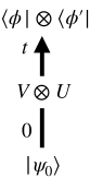
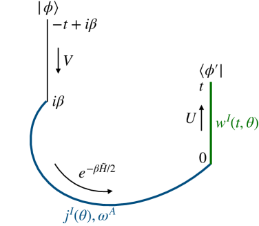
Figure 1: (Left) The evolution of (2.23) to (2.26). (Right) The contour $C$ in (2.38) to give the wave function of (2.26). The two vertical lines are the Lorentzian time-evolution over $[0,t]$ by $V$ and $U$, while the half curve is the Euclidean evolution over $[0,\beta/2]$. In the figure, the Lorentzian time direction of $V$ is drawn opposite to $U$, to match with figure 3.

2.2.2 Original state

Next, we find the path integral representation of the functional to generate (2.28). As will be shown in appendix A, the following holds for $\ket{\psi_{t}}$:

$${}_{\mathrm{L}}\bra{\phi}\otimes{}_{\mathrm{R}}\bra{\phi^{\prime}}V_{\mathrm{L}}(t)\otimes U_{\mathrm{R}}(t)\left(\sum_{n}\ket{n}_{\mathrm{L}}\otimes e^{-\beta\tilde{H}_{\mathrm{R}}/2}\ket{n}_{\mathrm{R}}\right)=\braket{\phi^{\prime}}{U(t)e^{-\beta\tilde{H}/2}V(t)}{\phi}.$$ (2.37)

Note that the l.h.s. is proportional to the wave function of the thermofield double state (2.23), and that the r.h.s. is written in terms of a single QFT. The r.h.s. can be expressed as

$$\braket{\phi^{\prime}}{U(t)e^{-\beta\tilde{H}/2}V(t)}{\phi}=\int_{\phi}^{\phi^{\prime}}\mathcal{D}\varphi\,e^{iI_{\mathrm{QFT}}[\varphi;C]},$$ (2.38)

where $C$ is the contour depicted in figure 1; first, $+t$ in the real direction, then $-i\beta$ in the pure imaginary direction, and finally $+t$ again in the real direction. The metric of the Lorentzian parts is (2.12), and the one for the Euclidean part is (2.34) with the replacement $\Omega^{A}\to\omega^{A}$. Regarding the continuity, the induced metric on constant time surface is the same between both metrics, but the extrinsic curvature is not analytically continuous. This is not a problem however, because there is no dynamical gravity on the QFT.

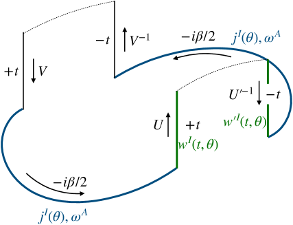
Figure 2: The contour $C^{\prime}$ for the generating functional (2.39). The source $w^{\prime}$ in the inverse contour is different from $w$, and $U^{\prime}$ is the time-evolution operator with source $w^{\prime}$. Note again that the Lorentzian time direction of $V$ and $V^{-1}$ is taken opposite to $U$ and $U^{\prime-1}$.

The generating functional to compute (2.28) is the path integral over the closed contour $C^{\prime}$ in figure 2:

$$Z_{C^{\prime}}[w,w^{\prime}]=\oint\mathcal{D}\varphi\,e^{iI_{\mathrm{QFT}}[\varphi;C^{\prime}]}.$$ (2.39)

In the arguments, $j$ and $\omega$ have been omitted, as they will be fixed hereafter. Since $C^{\prime}$ is closed, the path integral is subject to the (anti-)periodic boundary condition. This path integral corresponds to

$$\mathrm{Tr}\left[\left(U^{\prime}(t)e^{-\beta\tilde{H}/2}V(t)\right)^{\dagger}U(t)e^{-\beta\tilde{H}/2}V(t)\right],$$ (2.40)

and thus when $w^{\prime}=w$, it is equal to $Z_{0}$, i.e, $Z_{C^{\prime}}[w,w]=Z_{0}$. The relation we need is

$$\mathrm{Tr}\left(\rho_{t}O_{I}(\theta)\right)=\left.\frac{1}{i\sqrt{-\sigma}}\frac{\delta}{\delta w^{I}(t,\theta)}\ln Z_{C^{\prime}}[w,w^{\prime}]\right|_{w^{\prime}\to w}.$$ (2.41)

To compute the expectation values of $H$ and $P_{A}$, we need to include the stress tensor $T_{ab}(z)$ in the source term of the Lagrangian, coupled to the source $\delta\sigma^{ab}$ as $(1/2)\delta\sigma^{ab}T_{ab}$. This corresponds to that the Lagrangian (2.13), which defines the evolution $U(t)$, is replaced with

$$I_{\mathrm{QFT}}[w,\delta\sigma] =I_{\mathrm{QFT}}[w]-\frac{1}{2}\int\mathrm{d}^{d}z\sqrt{-\sigma}\,\delta\sigma^{ab}(z)T_{ab}(z)$$

$$=\int\mathrm{d}^{d}z\,\sqrt{-\mathrm{det}\left(\sigma_{ab}+\delta\sigma_{ab}\right)}\mathcal{L}[\sigma_{ab}+\delta\sigma_{ab}]+\int\mathrm{d}^{d}z\sqrt{-\sigma}\,w^{I}(z)O_{I}(z),$$ (2.42)

where $\delta\sigma_{ab}:=-\sigma_{ac}\sigma_{bd}\delta\sigma^{cd}$. Note that the metric in the source term is not perturbed. In the following, we include $-\delta\sigma^{ab}/2$ in $\{w^{I}\}$, so that we can deal with them collectively. In the expression (2.41), we take $\delta\sigma\to 0$ together with $w^{\prime}\to w$.

3 Description in gravity

Since the path integral representations (2.33) and (2.39) have been obtained, the GKPW formula enables us to write them in terms of gravity. Especially, (2.33) corresponds to a classical Euclidean gravity solution, and we will derive its thermodynamic laws. Our coarse-grained entropy is, in the classical limit, equal to the horizon area of the Euclidean cigar geometry (figure 4). The application to non-AdS cases is discussed at the end of this section.

3.1 Setup

Here, a $d$-dimensional holographic CFT is considered. The contents in section 2 apply as they are, and we use the holographic dictionary to rewrite them in the gravitational language. Particularly, we find the dual descriptions of the conditions (2.21) and the coarse-grained entropy $S(\rho_{\mathrm{ref},t})$.

The bulk configuration dual to (2.39) is constructed by the common procedure [60, 61]. As figure 12 of [61], the resulting spacetime fills the bulk of figure 2 as shown in figure 3. (In this figure, only the forward half is drawn, and it is up to the time slice drawn red that corresponds to the forward half of figure 2.) Our target is the unshaded single-sided black hole spacetime.

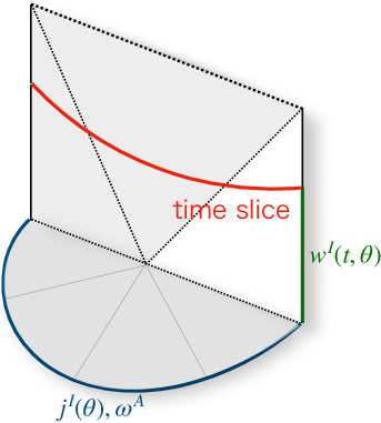
Figure 3: The bulk spacetime. The half disc depicts the Euclidean time evolution over $[0,\beta/2]$ to prepare the initial configuration at $t=0$, which evolves to the Lorentzian part drawn vertically. The dotted diagonal lines are the event horizons. This classical solution is constructed by properly joining the saddle point of each part [61].

Our setup and assumptions in the dual gravity are as follows:

• We consider that the bulk $M$ is governed by the Einstein gravity,

  $$I_{\mathrm{grav}}=\frac{1}{16\pi G}\int_{M}\mathrm{d}^{d+1}x\sqrt{-g}\,(R-2\Lambda)+\frac{1}{8\pi G}\int_{\partial M}\mathrm{d}^{d}z\sqrt{-\gamma}\,K+I_{\mathrm{matter}}+I_{\mathrm{ct}},$$ (3.1)

  where $I_{\mathrm{matter}}$ is the matter Lagrangian, $I_{\mathrm{ct}}$ is the counterterm both for gravity and matter, and $K_{ab}$ is the extrinsic curvature of the boundary and $K$ is its trace, $K:=\gamma^{ab}K_{ab}$. We assume that $I_{\mathrm{matter}}$ does not contain any boundary term.

• We write the bulk metric as

  $$\mathrm{d}s^{2}=g_{\mu\nu}\mathrm{d}x^{\mu}\mathrm{d}x^{\nu}=-N^{2}\mathrm{d}t^{2}+N_{r}^{2}\mathrm{d}r^{2}+c_{AB}\left(\mathrm{d}\theta^{A}+N^{A}\mathrm{d}t\right)\left(\mathrm{d}\theta^{B}+N^{B}\mathrm{d}t\right),$$ (3.2)

  with the gauge-fixing condition $g_{rt}=g_{rA}=0$. Throughout this paper, $\mu,\nu,\cdots$ are used for the bulk spacetime coordinates, $A,B,\cdots$ are for $\theta$-coordinates, and $a,b,\cdots$ are for the combination of $(t,\theta^{A})$.

• With the unit normal $\mathtt{u}_{\mu}\propto\partial_{\mu}t$ and the pull-back $e_{A}^{\mu}$, the vector of time direction is expressed as

  $$\mathtt{t}^{\mu}\partial_{\mu}:=\partial_{t}=(N\mathtt{u}^{\mu}+N^{A}e^{\mu}_{A})\partial_{\mu}=N\mathtt{u}^{a}\partial_{a}+N^{A}\partial_{A}.$$ (3.3)

• The boundary $\partial M$ is located at $r\to\infty$, where the induced metric of the Lorentzian part becomes (2.12) after the conformal factor is removed:

  $$\mathrm{d}s^{2}\sim\frac{r^{2}}{L^{2}}\left(-\mathrm{d}t^{2}+\sigma_{AB}\mathrm{d}\theta^{A}\mathrm{d}\theta^{B}\right)+N_{r}^{2}\mathrm{d}r^{2}.$$ (3.4)

  The induced metric on $r=\mathrm{const}$ is $\gamma_{ab}$, which asymptotes to the first term above.

• The on-shell value of the action is expressed as $I_{\mathrm{grav}}[w,w^{\prime}]$. The argument $w$ is the one appeared in (2.39), and related to the asymptotic value of the bulk fields $\Phi^{I}$ (including $g_{\mu\nu}$) as

  $$\Phi^{I}(x)\sim\left(\frac{R}{L}\right)^{\Delta_{I}-d}w^{I}(z)=:W^{I}(z),$$ (3.5)

  where $R$ is the IR cut-off to be sent $R\to\infty$, and $\Delta_{I}$ is the conformal dimension of $O_{I}$. The argument $w^{\prime}$ is related to $W^{\prime}$ in the same say in the backward evolution of figure 2.

• The counterterm $I_{\mathrm{ct}}$ is usually determined as [62, 63].

3.2 Coarse-graining conditions in the bulk

According to the the GKPW formula, (2.41) is rewritten as

$$\mathrm{Tr}\left(\rho_{t}O_{I}(\theta)\right)=\lim_{R\to\infty}\left(\frac{R}{L}\right)^{\Delta_{I}}\left.\frac{1}{\sqrt{-\gamma}}\frac{\delta I_{\mathrm{grav}}[w,w^{\prime}]}{\delta W^{I}(t,\theta)}\right|_{w^{\prime}\to w}.$$ (3.6)

For the stress tensor, in particular, we have

$$\mathrm{Tr}\left(\rho_{t}T_{ab}(\theta)\right)=\lim_{R\to\infty}\left(\frac{R}{L}\right)^{d-2}Y_{ab}(z),$$ (3.7)

where $Y_{ab}$ is the Brown-York tensor defined as [62]

$$Y_{ab}:=-\frac{2}{\sqrt{-\gamma}}\frac{\delta I_{\mathrm{grav}}}{\delta\gamma^{ab}}=\frac{1}{8\pi G}\left(K\gamma_{ab}-K_{ab}\right)-\frac{2}{\sqrt{-\gamma}}\frac{\delta I_{\mathrm{ct}}}{\delta\gamma^{ab}}.$$ (3.8)

Therefore, all we need is

$$\delta_{w}I_{\mathrm{grav}}[w]:= I_{\mathrm{grav}}[w+\delta w,w]-I_{\mathrm{grav}}[w,w]$$

$$= \int\mathrm{d}^{d+1}x\,(\mathrm{EOM})_{I}\delta_{w}\Phi^{I}+\int\mathrm{d}^{d}z\sqrt{-\gamma}\,\pi_{I}(z)\delta W^{I}(z).$$ (3.9)

Since we are interested in the on-shell variation, only the boundary terms remain. By definition, the Brown-York tensor is considered as

$$\pi_{I}=Y_{ab}\qquad\mathrm{for}\qquad\delta W^{I}=-\delta\gamma^{ab}/2.$$ (3.10)

When $I_{\mathrm{matter}}$ takes the form $\int\mathrm{d}^{d+1}x\sqrt{-g}\,\mathcal{L}_{\mathrm{matter}}(\Phi^{I^{\prime}},\nabla_{\mu}\Phi^{I^{\prime}};g)$ ($I^{\prime}$ does not contain $g_{\mu\nu}$), $\pi_{I^{\prime}}$ for the matter fields are written as

$$\pi_{I^{\prime}}=r_{\mu}\frac{\partial\mathcal{L}_{\mathrm{matter}}}{\partial\left(\nabla_{\mu}\Phi^{I^{\prime}}\right)}+\frac{1}{\sqrt{-\gamma}}\frac{\delta I_{\mathrm{ct}}}{\delta W^{I^{\prime}}}\qquad\mathrm{for}\qquad\delta W^{I^{\prime}}=\delta\Phi^{I^{\prime}}|_{r=R},$$ (3.11)

where $r_{\mu}=N_{r}^{-1}\delta_{\mu}^{r}$ is the unit normal of $r=\mathrm{const}$. As seen above, $\pi_{I}$ is like the “canonical conjugate momentum” (up to counterterm contributions) if $r$ were viewed as the time coordinate. This viewpoint agrees with the fact that differentiating the on-shell action with the final position generates the canonical conjugate momentum.

Therefore, (3.6) is reduced to

$$\mathrm{Tr}\left(\rho_{t}O_{I^{\prime}}(\theta)\right)=\lim_{R\to\infty}\left(\frac{R}{L}\right)^{\Delta_{I^{\prime}}}\pi_{I^{\prime}}(t,\theta)=:o_{I^{\prime},t}(\theta),$$ (3.12)

and (3.9) reproduces the on-shell variation formula:

$$\delta_{w}I_{\mathrm{grav}}[w]=\int\mathrm{d}^{d}z\sqrt{-\sigma}\,o_{I^{\prime},t}(\theta)\delta w^{I^{\prime}}(t,\theta)-\frac{1}{2}\int\mathrm{d}^{d}z\sqrt{-\gamma}\,Y_{ab}(t,\theta)\delta\gamma^{ab}(t,\theta).$$ (3.13)

For $H$ and $P_{A}$, the following holds from (2.15) and (3.7):

$$\mathrm{Tr}\left(\rho_{t}H\right)=\lim_{R\to\infty}\left(\frac{R}{L}\right)^{d-2}\int\mathrm{d}^{d-1}\theta\sqrt{-\sigma}\,u^{a}Y_{ab}t^{b}=\lim_{R\to\infty}\int\mathrm{d}^{d-1}\theta\sqrt{c}\,N\mathtt{u}^{a}Y_{ab}\mathtt{u}^{b}=:h_{t},$$ (3.14)

$$\mathrm{Tr}\left(\rho_{t}P_{A}\right)=\lim_{R\to\infty}\left(\frac{R}{L}\right)^{d-2}\int\mathrm{d}^{d-1}\theta\sqrt{-\sigma}\,u^{a}Y_{ab}e^{b}_{A}=\lim_{R\to\infty}\int\mathrm{d}^{d-1}\theta\sqrt{c}\,\mathtt{u}^{a}Y_{ab}e^{b}_{A}=:p_{A,t}.$$ (3.15)

Here, we have used $u^{a}=t^{a}\sim N\mathtt{u}^{a}$ as $r\to\infty$, which follows from (3.4).

It should be noted that $o_{I^{\prime}}$ and $Y_{ab}$ are evaluated by $I_{\mathrm{\mathrm{grav}}}[w,w]$ ($w^{\prime}$ is set to be $w$). According to [61], the bulk in such a case will be simply constructed as follows. First, we cut into half the dominant Euclidean black hole solution dual to $Z_{0}$ (see also next paragraph), which provides the Euclidean “half disc” in figure 3. Next, we solve the initial value problem from $t=0$, with the initial configuration given by analytically continuing the Euclidean solution. The initial values obtained in this way are compatible with constrains (e.g. Hamiltonian constraint). In solving this problem toward time $t$, the fields are subject to the Neumann boundary conditions specified by $w^{I}$ on $\partial M$. The backward evolution part is simply obtained by time-reversing it.

Next, we move on to the dual gravitational description for $\rho_{\mathrm{ref},t}$ in (2.18). We assume that the bulk solution that dominates $Z[\Gamma]$ does not depend on the imaginary time (i.e, stationary), and let $I_{\mathrm{grav}}^{(\mathrm{E})}[\Gamma]$ be the bulk Euclidean action evaluated by the dominant saddle point for given $\Gamma$. Similarly to the Lorentzian case, the same formulae hold for the Euclidean solution:

$$\mathrm{Tr}\left(\rho[\Gamma]O_{I^{\prime}}(\theta)\right)=\lim_{R\to\infty}\left(\frac{R}{L}\right)^{\Delta_{I^{\prime}}}\pi_{I^{\prime}}(\theta)=:o_{I^{\prime}}[\Gamma](\theta),$$ (3.16)

$$\mathrm{Tr}\left(\rho[\Gamma]H\right)=\lim_{R\to\infty}\int\mathrm{d}^{d-1}\theta\sqrt{\tilde{c}}\,N\mathtt{u}^{a}Y_{ab}\mathtt{u}^{b}=:h[\Gamma],$$ (3.17)

$$\mathrm{Tr}\left(\rho[\Gamma]P_{A}\right)=\lim_{R\to\infty}\int\mathrm{d}^{d-1}\theta\sqrt{\tilde{c}}\,\mathtt{u}^{a}Y_{ab}e^{b}_{A}=:p_{A}[\Gamma],$$ (3.18)

where, $\pi_{I^{\prime}}$ here is defined as

$$\pi_{I^{\prime}}(\theta):=-\frac{1}{B\sqrt{\tilde{\gamma}}}\frac{\delta I_{\mathrm{grav}}^{\left(\mathrm{E}\right)}[\Gamma]}{\delta\mathcal{J}^{I}(\theta)},\qquad\mathcal{J}^{I}(\theta):=\left(\frac{R}{L}\right)^{\Delta_{I^{\prime}}-d}J^{I}(\theta).$$ (3.19)

The tildes on the metrics indicates the Euclidean signature. As opposed to the Lorentzian case, the time vector is twisted as $\tau^{a}=u^{a}+i\Omega^{A}e_{A}^{a}$ due to $\Omega$ in (2.34). However, in order to measure $H$ rather than the Hamiltonian that generates $\tau$-translation of (2.34), we had to choose $u^{a}T_{ab}u^{b}$, not $u^{a}T_{ab}\tau^{b}$. This point has already been taken into account in (3.17).

From the above, (2.21) is equivalent in the bulk to finding the set $\Gamma=(B,\Omega,J)$ such that

$$o_{I^{\prime}}[\Gamma]=o_{I^{\prime},t}\qquad h[\Gamma]=h_{t},\qquad p_{A}[\Gamma]=p_{A,t}.$$ (3.20)

We write the solution as $\Gamma_{t}=(\beta_{t},\omega_{t},j_{t})$. The first condition is equivalent to equating the leading behaviors of $\pi_{I}$.

3.3 Coarse-grained entropy

After $\Gamma_{t}$ is found for each time $t$, our coarse-grained entropy can be computed in the gravity. We write the bulk metric as

$$\mathrm{d}s^{2}=\tilde{g}_{\mu\nu}\mathrm{d}x^{\mu}\mathrm{d}x^{\nu}=\tilde{N}^{2}\mathrm{d}\tau^{2}+\tilde{N}_{r}^{2}\mathrm{d}r^{2}+\tilde{c}_{AB}\left(\mathrm{d}\theta^{A}+i\tilde{N}^{A}\mathrm{d}\tau\right)\left(\mathrm{d}\theta^{B}+i\tilde{N}^{B}\mathrm{d}\tau\right),$$ (3.21)

similar to (3.2). We write the metric on $r=\mathrm{const}$ as $\tilde{\gamma}_{ab}$. This metric asymptotes to (2.34) as

$$\tilde{N}\sim\frac{r}{L},\qquad\tilde{N}^{A}\sim\Omega^{A},\qquad\tilde{c}_{AB}\sim\frac{r^{2}}{L^{2}}\sigma_{AB},\qquad(r\to\infty).$$ (3.22)

We suppose $\tilde{N}_{r}|_{r=r_{h}}=0$ and $\partial_{r}\tilde{N}_{r}|_{r=r_{h}}\neq 0$ for some $r_{h}>0$, as figure 4. In this case by a coordinate transformation $\mathrm{d}\rho=N_{r}\mathrm{d}r$ ($\rho(r_{h})=0$), the metric near $r=r_{h}$ must behave as

$$\mathrm{d}s^{2}\sim\mathrm{d}\rho^{2}+\left(\frac{2\pi}{B}\rho\right)^{2}\mathrm{d}\tau^{2}+\tilde{c}_{AB}\mathrm{d}\theta^{A}\mathrm{d}\theta^{B},$$ (3.23)

so as to avoid the conical singularity. Note that the shift vectors must also vanish (see below (2.34) and also section 3.5.2).

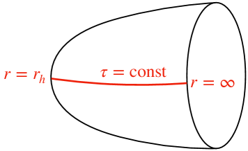
Figure 4: The Euclidean cigar geometry and a time slice $\tau=\mathrm{const}$.

First, the entropy of $\rho[\Gamma]$ in (2.30) is

$$S(\rho[\Gamma]) =-\mathrm{Tr}\left(\rho[\Gamma]\ln\rho[\Gamma]\right)$$

$$=\ln Z[\Gamma]+B\,\mathrm{Tr}\left(\rho[\Gamma]\left\{H-\Omega^{A}P_{A}-\int\mathrm{d}^{d-1}\theta\,\sqrt{-\sigma}J^{I}(\theta)O_{I}(\theta)\right\}\right)$$ (3.24)

$$=B^{2}\frac{\partial}{\partial B}\left(-B^{-1}\ln Z[\Gamma]\right).$$ (3.25)

Using the holographic dictionary, $-\ln Z[\Gamma]=I_{\mathrm{grav}}^{(\mathrm{E})}[\Gamma]$, we obtain

$$S(\rho[\Gamma])=I_{\mathrm{grav}}^{(\mathrm{E})}[\Gamma]-B\frac{\partial I_{\mathrm{grav}}^{(\mathrm{E})}[\Gamma]}{\partial B}=B\hat{\mathrm{d}}_{B}I_{\mathrm{grav}}^{(\mathrm{E})}[\Gamma],$$ (3.26)

where $\hat{\mathrm{d}}_{B}$ is $B$-derivative that acts only on the fields (with the integration range of $\tau$ fixed) and the last equation follows from the $\tau$-independence of the on-shell fields. Thus, $\hat{\mathrm{d}}_{B}I_{\mathrm{grav}}^{(\mathrm{E})}[\Gamma]$ is just the field variation triggered by $B$, and the Euclidean version of (3.9) can be used with $\delta_{w}\to\hat{\mathrm{d}}_{B}$. Since the bulk fields are subject to boundary conditions $J^{I}(\theta)$ independent of $B$, (3.9) seems to vanish. But, the variation perturbs $B$ in (3.23), generating a non-trivial conical singularity. Due to this, we have [65]

$$-\frac{1}{16\pi G}\int\mathrm{d}^{d+1}x\,\hat{\mathrm{d}}_{B}(\sqrt{\tilde{g}}\,R)=\frac{1}{4GB}\int_{r_{h}}\mathrm{d}^{d-1}\theta\sqrt{\tilde{c}}+\left(\mbox{regular terms}\right),$$ (3.27)

by which we obtain

$$S\left(\rho[\Gamma]\right)=\frac{1}{4G}\int_{r_{h}}\mathrm{d}^{d-1}\theta\sqrt{\tilde{c}}.$$ (3.28)

The fact that the entropy is given by the area of the tip agrees with [66], where the replica trick is used. If necessary, quantum corrections will be taken into consideration as in [28, 29, 30, 35].

3.4 Thermodynamic laws

The second law is guaranteed via the AdS/CFT correspondence by (2.22):

$$S(\rho[\Gamma_{t}])\geq S(\rho[\Gamma_{0}]).$$ (3.29)

Here, $S(\rho[\Gamma_{0}])$ coincides with the horizon area of the initial black hole, as we have set $\rho_{0}=\rho_{\mathrm{ref},0}$. Therefore, the horizon area of the auxiliary Euclidean black hole never gets smaller than the initial value.

Next, let us derive the first law. To find it, we perform a scaling transformation $\tau_{s}=B^{-1}\tau$. Values in the scaled coordinate is put subscript $s$ below. The periodicity is modified to $\tau_{s}+1\sim\tau_{s}$, and (3.22) and (3.23) are changed to

$$\tilde{N}_{s}\sim B\frac{r}{L},\qquad\tilde{N}^{A}_{s}\sim B\Omega^{A},\qquad(r\to\infty),$$ (3.30)

$$\mathrm{d}s^{2}\sim\mathrm{d}\rho^{2}+(2\pi\rho)^{2}\mathrm{d}\tau_{s}^{2}+\tilde{c}_{AB}\mathrm{d}\theta^{A}\mathrm{d}\theta^{B}\qquad(r=r_{h}).$$ (3.31)

In this coordinate, the derivative $\hat{\mathrm{d}}_{B}$ does not give any conical singularity, but this time it act on the boundary metric. In addition, the volume factors transformed as $\sqrt{\tilde{\gamma}_{s}}=B\sqrt{\tilde{\gamma}}$ and $\sqrt{\tilde{\sigma}_{s}}=B\sqrt{\tilde{\sigma}}$ while $Y_{ab}u^{a}u^{b}$ and $Y_{ab}u^{a}e^{b}_{A}$ are invariant. Noting those points, we take a variation $\delta\Gamma$ for $I_{\mathrm{grav}}^{(\mathrm{E})}[\Gamma]$ (see (2.35), (3.13) and (3.19)):

$$\delta_{\Gamma}I_{\mathrm{grav}}^{(\mathrm{E})}[\Gamma]= -\int\mathrm{d}^{d-1}\theta\sqrt{\tilde{\sigma}_{s}}\,o_{I^{\prime}}[\Gamma](\theta)\delta J^{I^{\prime}}(\theta)-\frac{1}{2}\int\mathrm{d}^{d-1}\theta\sqrt{\tilde{\gamma}_{s}}\,Y_{ab}(\theta)\delta_{\Gamma}\gamma^{ab}(\theta),$$ (3.32)

$$\delta_{\Gamma}\gamma_{ab}= \frac{2}{B}\left(\delta B\mathtt{u}_{a}\mathtt{u}_{b}-\delta(B\Omega^{A})\mathtt{u}_{a}e_{Ab}\right).$$ (3.33)

Therefore, going back to the original coordinate, we obtain

$$\delta_{\Gamma}I_{\mathrm{grav}}^{(\mathrm{E})}[\Gamma]=h[\Gamma]\delta B-p_{A}[\Gamma]\delta(B\Omega^{A})-\int\mathrm{d}^{d-1}\theta\sqrt{\tilde{\sigma}}\,\hat{o}_{I^{\prime}}[\Gamma](\theta)\delta J^{I^{\prime}}(\theta),$$ (3.34)

where we have defined

$$\hat{o}_{I^{\prime}}[\Gamma]:=Bo_{I^{\prime}}[\Gamma].$$ (3.35)

In (3.34), we have supposed that $\{\Phi^{I^{\prime}}\}$ includes only fields that are invariant under the scaling. Soon later, we will see what happens if there are scaling fields such as the Maxwell field.

The entropy function is obtained by the Legendre transformation from $\Gamma$ to $\Xi:=(h,p,\hat{o})$:

$$S[\Xi]:= B[\Xi]\left(h-p_{A}\Omega^{A}[\Xi]\right)-\int\mathrm{d}^{d-1}\theta\sqrt{\tilde{\sigma}}\,\hat{o}_{I^{\prime}}(\theta)J^{I^{\prime}}[\Xi](\theta)-I_{\mathrm{grav}}^{(\mathrm{E})}[\Gamma[\Xi]]$$ (3.36)

$$\delta_{\Xi}S[\Xi]= B[\Xi]\left(\delta h-\Omega^{A}[\Xi]\delta p_{A}\right)-\int\mathrm{d}^{d-1}\theta\sqrt{\tilde{\sigma}}\,\delta\hat{o}_{I^{\prime}}(\theta)J^{I^{\prime}}[\Xi](\theta).$$ (3.37)

Now, the entropy has a new expression (3.36), which is seemingly different from (3.28). But, they must be equivalent:

$$S(\rho[\Gamma_{t}])=S[\Xi_{t}],\qquad\Xi_{t}:=(h_{t},p_{t},\hat{o}_{t}).$$ (3.38)

As a matter of fact, (3.36) is exactly the same as the corresponding CFT expression (3.24). By construction of $\Gamma_{t}$, the argument $\Xi_{t}$ is the one given in (3.12), (3.14), and (3.15) up to the hat symbol. The first law follows from (3.37):

$$\dot{S}[\Xi_{t}]=B[\Xi_{t}]\left(\dot{h}_{t}-\Omega^{A}[\Xi_{t}]\dot{p}_{A,t}\right)-\int\mathrm{d}^{d-1}\theta\sqrt{\tilde{\sigma}}\,\dot{\hat{o}}_{I^{\prime},t}(\theta)J^{I^{\prime}}[\Xi](\theta).$$ (3.39)

This equation contains the local terms from matter fields, in addition to the usual first law.

Finally, let us see how (3.34) and below are modified when there are scaling fields. To be concrete, we demonstrate with the time component of $\mathrm{U}(1)$ gauge field $A_{0}$, whose $J^{I}$ and $o_{I}$ we write as $a$ and $q$, respectively. In this case, (3.34) is modified to

$$\delta_{\Gamma}I_{\mathrm{grav}}^{(\mathrm{E})}[\Gamma]=\eqref{eq: unscaled variation}-\int\mathrm{d}^{d-1}\theta\sqrt{\tilde{\sigma}}\,q[\Gamma](\theta)\delta(Ba(\theta)).$$ (3.40)

Accordingly, $q$ is added to $\Xi$, and (3.36) and (3.39) acquire additional terms:

$$S[\Xi]:= ~{}\eqref{eq: entropy function}-B[\Xi]\int\mathrm{d}^{d-1}\theta\sqrt{\tilde{\sigma}}\,q(\theta)a[\Xi](\theta),$$ (3.41)

$$\dot{S}[\Xi_{t}]= ~{}\eqref{eq: first law}-B[\Xi_{t}]\int\mathrm{d}^{d-1}\theta\sqrt{\tilde{\sigma}}\,\dot{q}_{t}(\theta)a[\Xi_{t}](\theta).$$ (3.42)

The additional term is the usual term consisting of the $\mathrm{U}(1)$ electric charge and the gauge potential, except that they are locally treated in the current case. If there are more fields scaled by $\tau_{s}=B^{-1}\tau$, similar terms are added depending on their transformation rules.

3.5 Comments on generalizations

3.5.1 Non-AdS cases

We have obtained the definition of our coarse-grained entropy purely in the gravitational language. If gravity is in general holographic in the sense that the quantum theory behind it is defined by specifying the boundary as assumed in [66], then we would reach the same results in the classical limit from the saddle point approximation applied to the fomal path integral of the quantum gravity. Thus, it is expected that the first and second law also holds for non-AdS cases.

Let us consider the Einstein gravity (3.1) on a Lorentzian manifold $M$ with a timelike boundary $\partial M$. The induced metric on $\partial M$ is assumed static, but the boundary conditions for the other bulk fields can depend on the time. Then, (3.20) determines the reference Euclidean solution on each time, whose horizon area is the entropy we want. In solving (3.20), the Brown-York tensor is defined in the same way, and the matching condition of $o_{I}$ is replaced with the matching of the leading term of $\pi_{I}$.

3.5.2 Choice of shift vectors

So far, we have adopted (2.34) as our gauge choice. As has been explained, it is possible to choose (2.36), where $\vartheta$ is shifted in the pure imaginary direction along with the $\tau$-periodicity. If we had taken this gauge, (3.23) would be changed to

$$\mathrm{d}s^{2}\sim\mathrm{d}\rho^{2}+\left(\frac{2\pi}{B}\rho\right)^{2}\mathrm{d}\tau^{2}+\tilde{c}_{AB}(\mathrm{d}\vartheta^{A}-i\Omega^{A}\mathrm{d}\tau)(\mathrm{d}\vartheta^{B}-i\Omega^{B}\mathrm{d}\tau),$$ (3.43)

from the requirement of removing the conical singularity. Seemingly different, but physically same results must be reproduced also in this gauge. A difference, for example, is that the (angular) momenta are measured not on the boundary, but at $r=r_{h}$. In fact, $\Omega$ does not appear in (3.33), but in (3.23) as above, and hence $B$ enters to (3.31) accompanying $\Omega$ when $\tau$ is scaled.

It was addressed in [67] for Kerr-AdS₅ spacetime, how the choice of the shift vectors affect on the first law. Since we allow matter fields to exist, the story seems to be not so simple as [67]. In vacuum solutions, for example, the angular momentum (Komar integral) measured at infinity is equal to the one at the horizon by the Stokes’ theorem, but different by the volume integral when matter exists. Nevertheless, the first law will be properly derived in a similar way.

4 Demonstration in Vaidya-type spacetimes

In this section, we check thermodynamic laws derived in the previous section for null-ray collapse models. Since the second law was predicted from the CFT, it provides an energy constraint for those examples.

4.1 Schwarzschild-AdS_d+1

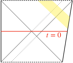
Figure 5: Vaidya-Schwarzschild-AdS_d+1 spacetime. At $t=0$, the Schwarzschild-AdS spacetime is prepared, and null rays exist in the yellow region.

Let us start with the simplest case where a null-ray is shot from the boundary to the Schwarzschild-AdS_d+1 spacetime. The initial metric is given as

$$\mathrm{d}s^{2}=-f(r)\mathrm{d}t^{2}+\frac{\mathrm{d}r^{2}}{f(r)}+r^{2}\mathrm{d}\Theta^{2},\qquad f(r):=1+\frac{r^{2}}{L^{2}}-\frac{2\mu(0)}{r^{d-2}},$$ (4.1)

where $\mathrm{d}\Theta^{2}$ is the metric of the unit $(d-1)$-dimensional sphere. The boundary metric with the conformal factor removed is

$$\mathrm{d}s^{2}|_{\mathrm{bdy}}=\mathrm{d}t^{2}+r^{2}\mathrm{d}\Theta^{2}.$$ (4.2)

The metric describing the null ray is

$$\mathrm{d}s^{2}=-f(v,r)\mathrm{d}v^{2}+2\mathrm{d}v\mathrm{d}r+r^{2}\mathrm{d}\Theta^{2},\qquad f(v,r)=1+\frac{r^{2}}{L^{2}}-\frac{2\mu(v)}{r^{d-2}}.$$ (4.3)

At the boundary, both time coordinates coincide, namely, $t=v$. In the bulk, the time coordinate $t$ is properly extended towards the future, but we do not concretely specify the foliation, since only the boundary observables at time $t$ are required in coarse-graining. Hence, we use $v$ for the time coordinate hereafter.

We take the mass $h_{v}$ as the only respected observable on the boundary. The mass $h_{v}$ depends on the counterterm [62, 63], but most of time [62], it is computed as

$$h_{v}=\frac{d-1}{8\pi G}\mathrm{Vol}\left(\mathbb{S}^{d-1}\right)\mu(v)+\left(\mbox{independent of $v$}\right).$$ (4.4)

The Euclidean black hole that minimizes the Euclidean action, having the same mass, will be

$$\mathrm{d}s^{2}=f(v,r)\mathrm{d}\tau^{2}+\frac{\mathrm{d}r^{2}}{f(v,r)}+r^{2}\mathrm{d}\Theta^{2}.$$ (4.5)

Note that $\tau$ is not related to the Lorentzian time $v$, but just the imaginary time for the reference Euclidean solution that we refer to at time $v$. It is explicitly confirmed that this geometry has the mass $h_{v}$. The Lagrange multiplier $\beta_{v}$ is found to be

$$\beta_{v}=\frac{4\pi}{\partial_{r}f(t,r_{h}(v))},$$ (4.6)

where $r=r_{h}(v)$ is the largest root of $f(v,r)$, related to $\mu(v)$ as

$$\mu(v)=\frac{1}{2}r_{h}(v)^{d-2}\left(1+\frac{r_{h}(v)^{2}}{L^{2}}\right).$$ (4.7)

The coarse-grained entropy is the area of the cigar tip,

$$S_{v}=\frac{\mathrm{Vol}\left(\mathbb{S}^{d-1}\right)}{4G}r_{h}(v)^{d-1}.$$ (4.8)

We see that the first law is satisfied:

$$\dot{S}_{v}=\beta_{v}\dot{h}_{v}.$$ (4.9)

On the other hand, the second law $S_{v}\geq S_{0}$ is equivalent to $r_{h}(v)\geq r_{h}(0)$, which is not satisfied for generic $\mu(v)$. We rather see this fact as a constraint from quantum gravity, since this must be satisfied in the dual description.

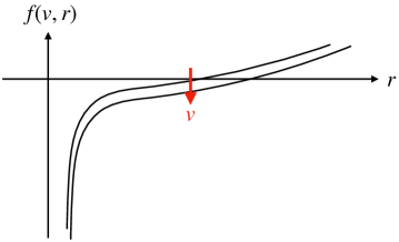
Figure 6: The behavior of $f(v,r)$ under the null energy condition.

Actually, the second law is satisfied when the null energy condition holds. The energy flow along a null vector $\ell=\partial_{v}+(f(v,r)/2)\partial_{r}$ is

$$T_{\ell\ell}:=T_{\mu\nu}\ell^{\mu}\ell^{\nu}\propto-\partial_{v}f(v,r).$$ (4.10)

If $T_{\ell\ell}\geq 0$, then $f(v,r)$ decreases in $v$, which implies that $r_{h}(v)$ increases (see figure 6). However, this monotonicity is stronger than required by our second law, and the following integrated version is sufficient for only saying $r_{h}(v)\geq r_{h}(0)$:

$$\forall v>0,\qquad\int_{0}^{v}\mathrm{d}v\,T_{\ell\ell}\geq 0.$$ (4.11)

4.2 Rotating BTZ

Next, we consider the uncharged BTZ spacetime and add the angular momentum $p_{\phi}$ to the respected observable set. The metric with null ray is given as

$$\mathrm{d}s^{2} =-N(v,r)^{2}\mathrm{d}v^{2}+2\mathrm{d}v\mathrm{d}r+r^{2}(\mathrm{d}\phi+N^{\phi}(v,r)\mathrm{d}v)^{2},$$ (4.12)

$$N(v,r)^{2} =-8Gm(v)+\frac{r^{2}}{L^{2}}+\frac{16G^{2}j(v)^{2}}{r^{2}},\qquad N^{\phi}(v,r)=\frac{4Gj(v)}{r^{2}}.$$ (4.13)

The boundary metric is again (4.2) with $\mathrm{d}\Theta^{2}=\mathrm{d}\phi^{2}$. We assume that $N(v,r)^{2}$ has two positive roots, i.e, $L^{2}m(v)^{2}>j(v)^{2}$, and the larger one is

$$r_{h}(v)=\left[4L^{2}Gm(v)\left(1+\sqrt{1-\frac{j(v)^{2}}{L^{2}m(v)^{2}}}\right)\right]^{1/2}.$$ (4.14)

The counterterm for gravity in $d=2$ [62, 63] is known as

$$I_{\mathrm{ct}}=-\frac{1}{8\pi GL}\int\mathrm{d}^{2}z\sqrt{-\gamma},$$ (4.15)

with which the mass and angular momentum are calculated as

$$h_{v}=m(v),\qquad p_{\phi,v}=j(v).$$ (4.16)

In considering the reference Euclidean geometry at $v$, we have two parameters $\beta_{v}$ and $\omega^{\phi}_{v}$. The metric that has $h_{v}$ and $p_{\phi,v}$, and is compatible with the boundary metric (2.34), is found to be

$$\mathrm{d}s^{2}= N(v,r)^{2}\mathrm{d}\tau^{2}+\frac{\mathrm{d}r^{2}}{N(v,r)^{2}}+r^{2}\left(\mathrm{d}\phi-i\hat{N}^{\phi}(v,r)\mathrm{d}\tau\right)^{2},$$ (4.17)

$$\hat{N}^{\phi}(v,r):= N^{\phi}(v,r)-N^{\phi}(v,r_{h}(v)).$$ (4.18)

Thus, the parameters are determined as

$$\beta_{v}=\frac{4\pi}{\partial_{r}N(v,r_{h}(v))^{2}},\qquad\omega^{\phi}_{v}=N^{\phi}(v,r_{h}(v)).$$ (4.19)

The coarse-grained entropy is

$$S_{v}=\frac{\pi}{2G}r_{h}(v),$$ (4.20)

and the first law holds as

$$\dot{S}_{v}=\beta_{v}(\dot{h}_{v}-\omega^{\phi}_{v}\dot{p}_{\phi,v}).$$ (4.21)

The second law means $r_{h}(v)\geq r_{h}(0)$. Again, this is guaranteed under the null energy condition (4.11) for a null vector $\ell=\partial_{v}+(N^{2}/2)\partial_{r}-N^{\phi}\partial_{\phi}$, by the same logic.

4.3 Reissner-Nordström (4d flat)

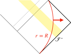
Figure 7: Vaidya-Bonner spacetime. The boundary is sent to infinity.

The final example is a 4-dimensional charged black hole. The solution we consider is the Vaidya-Bonner spacetime,

$$\mathrm{d}s^{2}= -N(v,r)^{2}\mathrm{d}v^{2}+2\mathrm{d}v\mathrm{d}r+r^{2}\mathrm{d}\Theta^{2},\qquad N(v,r)^{2}=1-\frac{2Gm(v)}{r}+\frac{Gq(v)^{2}}{4\pi r^{2}},$$ (4.22)

$$A= -\frac{q(v)}{2\pi r}\left(\mathrm{d}v-\frac{\mathrm{d}r}{N(v,r)^{2}}\right),$$ (4.23)

where $\mathrm{d}\Theta^{2}=\mathrm{d}\theta^{2}+\sin^{2}\theta\mathrm{d}\phi^{2}$, and $r_{h}(v)$ is the largest root of $N(v,r)^{2}$ given as

$$r_{h}(v)=Gm(v)+\sqrt{(Gm(v))^{2}-\frac{Gq(v)^{2}}{4\pi}},$$ (4.24)

with the quantity in the square root assumed positive. We choose $r=R$ as the boundary, whose induced metric is

$$\mathrm{d}s^{2}|_{\mathrm{bdy}}=-N(v,R)^{2}\mathrm{d}v^{2}+R^{2}\mathrm{d}\Theta^{2}.$$ (4.25)

Since this induced metric is time-dependent, we send $R$ to infinity, in order for it to be time-independent. This infinity corresponds to the past null infinity $\mathscr{I}^{-}$. This time, the respected quantities are the mass and the electric charge. Observed at $\mathscr{I}^{-}$, the mass and charge are

$$h_{v}=m(v),\qquad q_{v}=q(v),$$ (4.26)

where the counterterm is, as usual, taken to be the contribution from the Minkowski spacetime. The mass is the Bondi-Sachs type mass.

The reference Euclidean spacetime is

$$\mathrm{d}s^{2}=N(v,r)^{2}\mathrm{d}\tau^{2}+\frac{\mathrm{d}r^{2}}{N(v,r)^{2}}+r^{2}\mathrm{d}\Theta^{2},\qquad A=-\frac{q(v)}{2\pi}\left(\frac{1}{r}-\frac{1}{r_{h}(v)}\right)\mathrm{d}\tau,$$ (4.27)

with the Lagrange multipliers given by

$$\beta_{t}=\frac{4\pi}{\partial_{r}N(v,r_{h}(v))^{2}},\qquad\lambda_{t}=\frac{1}{2\pi}A_{\tau}|_{r\to\infty},$$ (4.28)

where $\lambda_{t}$ is the conjugate of $q_{v}$.

The entropy is, hence,

$$S_{v}=\frac{\pi}{G}r_{h}(v)^{2}.$$ (4.29)

The first law is satisfied in the form (3.42):

$$\dot{S}_{v}=\beta_{v}(\dot{h}_{v}-\lambda_{v}\dot{q}_{v}).$$ (4.30)

The second law again implies (4.11), with $\ell=\partial_{v}+(N^{2}/2)\partial_{r}$.

If we decide not to respect the charge, the resulting entropy must become larger. This choice is possible when $q(0)=0$, necessary for $S_{0}$ to coincide with the initial entropy. In this case, the reference Euclidean geometry would be

$$\mathrm{d}s^{2}=f(v,r)\mathrm{d}\tau^{2}+\frac{\mathrm{d}r^{2}}{f(v,r)}+r^{2}\mathrm{d}\Theta^{2},\qquad f(v,r)=1-\frac{2Gm(v)}{r}.$$ (4.31)

Then, the horizon radius is $2Gm(v)$, which is larger than $r_{h}(v)$, and hence the entropy becomes larger as well. This reflects the fact that coarse-grained entropy increases when fewer constraints are imposed.

5 Discussions

We have introduced a coarse-grained entropy that respects asymptotic values on each time slice, as a new measure of black hole thermodynamics. The entropy is the horizon area of a specific reference Euclidean black hole, faithful to the first and second laws. The second law, proven from the CFT, is expected to be a reflection of the thermal (or statistical) nature of quantum gravity. As a matter of fact, the second law is not always satisfied, providing a constraint on gravity. Through several examples, we have discovered that the constraint seems to be related to the integrated null energy condition.

The coarse-grained entropy introduced in this paper has its definition both on the boundary and in the bulk. As a newly established dictionary, this will enable us to study the non-equilibrium process from CFT to gravity, and vice versa. Although we have focused on the thermodynamics of gravity in this paper, it is of course possible to survey the evolution of the coarse-grained entropy in the CFT from the bulk analysis.

While the first law was derived within the Einstein gravity, we asked for the help of the holographic dictionary in showing the second law. It is valuable to further survey what the second law means in more complex situations, since the second law seems to imply something that the Einstein theory itself does not tell. Particularly, we did not specify the origin of the null rays in Vaidya models, but if it were possible, we could add the matter fields to the set of respected quantities. For this purpose, the solution in [69], which offers a null ray collapse model within given fields, will be helpful.

It is also interesting to consider other ways of coarse-graining to provide some thermodynamic constraints. In our coarse-graining process, especially, only the boundary observables on the time slice are referred to at each time $t$, and hence it does not tell any difference that happens deep inside the bulk. To be more finely grained, the coarse-grained state must also respect observables off the time slice. By doing so, the information of some codimension-0 domain on the boundary is kept, preserving some bulk region causally related to it. This idea has been addressed in the literature [40, 45, 47].

Finally, one of the aims of non-equilibrium thermodynamics is to describe the relaxation process. If there is non-equilibrium thermodynamics in gravity, does it also have knowledge about the relaxation of gravitational systems? In some sense, we can say that the no-hair theorem teaches what states are possible as the final states, after matter has fallen behind the horizon. However, it is still a mystery how the system evolves to the final state, or whether the fate of the system must be thermodynamically controlled. We expect that studying non-equilibrium black hole thermodynamics will reveal those problems.

Acknowledgement

I thank Masafumi Fukuma, Osamu Fukushima, Yuji Hirono, Takanori Ishii, Tomohiro Shigemura, Keito Shimizu, Sotaro Sugishita, Ryota Watanabe, and Takuya Yoda for discussion. I am also grateful for daily advice by Koji Hashimoto and Shigeki Sugimoto. My work was supported by Grant-in-Aid for JSPS Fellows No. 22KJ1944.

Appendix A Derivation of (2.37)

We derive (2.37) in this appendix. We denote the r.h.s. as $T$, and will show that $T$ is deformed to the l.h.s. In the following, the CPT operator $\Theta$ plays a key role. The CPT conjugate state $\bra{\Theta\psi}$ of a state $\ket{\psi}$ is defined as

$$\forall\ket{\psi^{\prime}},\qquad\braket{\Theta\psi}{\psi^{\prime}}=(\braket{\psi^{\prime}}{\Theta}{\psi})^{*},$$ (A.1)

where the asterisk means the complex conjugation. Note that $\Theta$ is antiunitary.

With $\Theta$ and any orthonormal basis $\{\ket{n}\}$, $T$ is deformed as follows:

$$T= \braket{\phi^{\prime}}{U(t)e^{-\beta\tilde{H}/2}\Theta^{\dagger}\Theta V(t)}{\phi}=\bra{\phi^{\prime}}U(t)e^{-\beta\tilde{H}/2}\Theta^{\dagger}\left(\sum_{n}\ket{n}\bra{n}\Theta V(t)\ket{\phi}\right)$$

$$= \sum_{n}\braket{n}{\Theta V(t)}{\phi}^{*}\braket{\phi^{\prime}}{U(t)e^{-\beta\tilde{H}/2}}{n_{\Theta}}.$$ (A.2)

Here, we have set $\ket{n_{\Theta}}:=\Theta^{\dagger}\ket{n}$. Assuming that the theory without sources is CPT-invariant, i.e, $H$ in (2.24) is invariant, we obtain

$$\braket{n}{\Theta V(t)}{\phi}^{*}=\braket{n}{V(t)^{\dagger}\Theta}{\phi}^{*}=\braket{\Theta\phi}{V(t)}{n}.$$ (A.3)

In addition, being a c-number, this can be seen calculated in a copied Hilbert space, which we call as QFT_L. The remaining part is kept in the original Hilbert space, QFT_R. Therefore we conclude

$$T={}_{\mathrm{L}}\bra{\Theta\phi}\otimes{}_{\mathrm{R}}\bra{\phi^{\prime}}V_{\mathrm{L}}(t)\otimes U_{\mathrm{R}}(t)\left(\sum_{n}\ket{n}_{\mathrm{L}}\otimes e^{-\beta\tilde{H}_{\mathrm{R}}/2}\ket{n_{\Theta}}_{\mathrm{R}}\right).$$ (A.4)

In this expression, $\bra{\Theta\phi}$ and $\ket{n_{\Theta}}$ appear, instead of $\bra{\phi}$ and $\ket{n}$. However, those differences do not matter. First, $\phi$ is just a dummy variable in the generating functional (2.39). Second, either $\ket{n}$ or $\ket{n_{\Theta}}$ can guarantee (2.28), meaning that we could have started from (2.23) with $\ket{n}_{\mathrm{R}}\to\ket{n_{\Theta}}_{\mathrm{R}}$ and reach the same results in the main text. Thus, for simplicity, we have ignored those subtleties in (2.37).

References

- [1] J.M. Bardeen, B. Carter and S.W. Hawking, The four laws of black hole mechanics, Communications in Mathematical Physics 31 (1973) 161.
- [2] S.W. Hawking and J.B. Hartle, Energy and angular momentum flow into a black hole, Communications in Mathematical Physics 27 (1972) 283.
- [3] R.M. Wald, Black hole entropy is the Noether charge, Phys. Rev. D 48 (1993) R3427 [gr-qc/9307038].
- [4] J.D. Bekenstein, Black holes and the second law, Lettere al Nuovo Cimento (1971-1985) 4 (1972) 737.
- [5] T. Jacobson, Thermodynamics of space-time: The Einstein equation of state, Phys. Rev. Lett. 75 (1995) 1260 [gr-qc/9504004].
- [6] S.W. Hawking, Particle creation by black holes, Communications in Mathematical Physics 43 (1975) 199.
- [7] A. Strominger and C. Vafa, Microscopic origin of the Bekenstein-Hawking entropy, Phys. Lett. B 379 (1996) 99 [hep-th/9601029].
- [8] S.W. Hawking, Black holes in general relativity, Communications in Mathematical Physics 25 (1972) 152.
- [9] J.D. Bekenstein, Black holes and entropy, Phys. Rev. D 7 (1973) 2333.
- [10] J.D. Bekenstein, Generalized second law of thermodynamics in black-hole physics, Phys. Rev. D 9 (1974) 3292.
- [11] A.C. Wall, Ten Proofs of the Generalized Second Law, JHEP 06 (2009) 021 [0901.3865].
- [12] S. Carlip, Black Hole Thermodynamics, Int. J. Mod. Phys. D 23 (2014) 1430023 [1410.1486].
- [13] A.C. Wall, A Survey of Black Hole Thermodynamics, 1804.10610.
- [14] S. Sarkar, Black Hole Thermodynamics: General Relativity and Beyond, Gen. Rel. Grav. 51 (2019) 63 [1905.04466].
- [15] R.M. Wald, “nernst theorem” and black hole thermodynamics, Phys. Rev. D 56 (1997) 6467.
- [16] C. Kehle and R. Unger, Gravitational collapse to extremal black holes and the third law of black hole thermodynamics, 2211.15742.
- [17] G. ’t Hooft, Dimensional reduction in quantum gravity, Conf. Proc. C 930308 (1993) 284 [gr-qc/9310026].
- [18] L. Susskind, The World as a hologram, J. Math. Phys. 36 (1995) 6377 [hep-th/9409089].
- [19] R. Bousso, The Holographic principle for general backgrounds, Class. Quant. Grav. 17 (2000) 997 [hep-th/9911002].
- [20] R. Bousso, The Holographic principle, Rev. Mod. Phys. 74 (2002) 825 [hep-th/0203101].
- [21] J.M. Maldacena, The Large N limit of superconformal field theories and supergravity, Adv. Theor. Math. Phys. 2 (1998) 231 [hep-th/9711200].
- [22] E. Witten, Anti-de Sitter space and holography, Adv. Theor. Math. Phys. 2 (1998) 253 [hep-th/9802150].
- [23] S.S. Gubser, I.R. Klebanov and A.M. Polyakov, Gauge theory correlators from noncritical string theory, Phys. Lett. B 428 (1998) 105 [hep-th/9802109].
- [24] S. Ryu and T. Takayanagi, Holographic derivation of entanglement entropy from AdS/CFT, Phys. Rev. Lett. 96 (2006) 181602 [hep-th/0603001].
- [25] S. Ryu and T. Takayanagi, Aspects of Holographic Entanglement Entropy, JHEP 08 (2006) 045 [hep-th/0605073].
- [26] V.E. Hubeny, M. Rangamani and T. Takayanagi, A Covariant holographic entanglement entropy proposal, JHEP 07 (2007) 062 [0705.0016].
- [27] A.C. Wall, Maximin Surfaces, and the Strong Subadditivity of the Covariant Holographic Entanglement Entropy, Class. Quant. Grav. 31 (2014) 225007 [1211.3494].
- [28] T. Barrella, X. Dong, S.A. Hartnoll and V.L. Martin, Holographic entanglement beyond classical gravity, JHEP 09 (2013) 109 [1306.4682].
- [29] T. Faulkner, A. Lewkowycz and J. Maldacena, Quantum corrections to holographic entanglement entropy, JHEP 11 (2013) 074 [1307.2892].
- [30] N. Engelhardt and A.C. Wall, Quantum Extremal Surfaces: Holographic Entanglement Entropy beyond the Classical Regime, JHEP 01 (2015) 073 [1408.3203].
- [31] G. Penington, Entanglement Wedge Reconstruction and the Information Paradox, JHEP 09 (2020) 002 [1905.08255].
- [32] A. Almheiri, N. Engelhardt, D. Marolf and H. Maxfield, The entropy of bulk quantum fields and the entanglement wedge of an evaporating black hole, JHEP 12 (2019) 063 [1905.08762].
- [33] A. Almheiri, R. Mahajan, J. Maldacena and Y. Zhao, The Page curve of Hawking radiation from semiclassical geometry, JHEP 03 (2020) 149 [1908.10996].
- [34] G. Penington, S.H. Shenker, D. Stanford and Z. Yang, Replica wormholes and the black hole interior, JHEP 03 (2022) 205 [1911.11977].
- [35] A. Almheiri, T. Hartman, J. Maldacena, E. Shaghoulian and A. Tajdini, Replica Wormholes and the Entropy of Hawking Radiation, JHEP 05 (2020) 013 [1911.12333].
- [36] D.N. Page, Information in black hole radiation, Phys. Rev. Lett. 71 (1993) 3743 [hep-th/9306083].
- [37] D.N. Page, Time Dependence of Hawking Radiation Entropy, JCAP 09 (2013) 028 [1301.4995].
- [38] K. Hashimoto, N. Iizuka and Y. Matsuo, Islands in Schwarzschild black holes, JHEP 06 (2020) 085 [2004.05863].
- [39] T. Takayanagi and T. Ugajin, Measuring Black Hole Formations by Entanglement Entropy via Coarse-Graining, JHEP 11 (2010) 054 [1008.3439].
- [40] W.R. Kelly and A.C. Wall, Coarse-grained entropy and causal holographic information in AdS/CFT, JHEP 03 (2014) 118 [1309.3610].
- [41] W.R. Kelly, Deriving the First Law of Black Hole Thermodynamics without Entanglement, JHEP 10 (2014) 192 [1408.3705].
- [42] V.E. Hubeny and M. Rangamani, Causal Holographic Information, JHEP 06 (2012) 114 [1204.1698].
- [43] B. Freivogel and B. Mosk, Properties of Causal Holographic Information, JHEP 09 (2013) 100 [1304.7229].
- [44] N. Engelhardt and A.C. Wall, No Simple Dual to the Causal Holographic Information?, JHEP 04 (2017) 134 [1702.01748].
- [45] N. Engelhardt and A.C. Wall, Decoding the Apparent Horizon: Coarse-Grained Holographic Entropy, Phys. Rev. Lett. 121 (2018) 211301 [1706.02038].
- [46] B. Grado-White and D. Marolf, Marginally Trapped Surfaces and AdS/CFT, JHEP 02 (2018) 049 [1708.00957].
- [47] N. Engelhardt and A.C. Wall, Coarse Graining Holographic Black Holes, JHEP 05 (2019) 160 [1806.01281].
- [48] J. Chandra and T. Hartman, Coarse graining pure states in AdS/CFT, JHEP 10 (2023) 030 [2206.03414].
- [49] D.D. Blanco, H. Casini, L.-Y. Hung and R.C. Myers, Relative Entropy and Holography, JHEP 08 (2013) 060 [1305.3182].
- [50] S. Banerjee, A. Bhattacharyya, A. Kaviraj, K. Sen and A. Sinha, Constraining gravity using entanglement in AdS/CFT, JHEP 05 (2014) 029 [1401.5089].
- [51] S. Banerjee, A. Kaviraj and A. Sinha, Nonlinear constraints on gravity from entanglement, Class. Quant. Grav. 32 (2015) 065006 [1405.3743].
- [52] N. Lashkari, C. Rabideau, P. Sabella-Garnier and M. Van Raamsdonk, Inviolable energy conditions from entanglement inequalities, JHEP 06 (2015) 067 [1412.3514].
- [53] C. Jarzynski, Nonequilibrium equality for free energy differences, Physical Review Letters 78 (1997) 2690.
- [54] C. Jarzynski, Hamiltonian derivation of a detailed fluctuation theorem, Journal of Statistical Physics 98 (2000) 77.
- [55] D.J. Evans, E.G.D. Cohen and G.P. Morriss, Probability of second law violations in shearing steady states, Physical review letters 71 (1993) 2401.
- [56] J. Kurchan, Fluctuation theorem for stochastic dynamics, Journal of Physics A: Mathematical and General 31 (1998) 3719.
- [57] H. Tasaki, Jarzynski relations for quantum systems and some applications, arXiv preprint cond-mat/0009244 (2000) .
- [58] M. Esposito, K. Lindenberg and C. Van den Broeck, Entropy production as correlation between system and reservoir, New Journal of Physics 12 (2010) 013013.
- [59] T. Sagawa, Second Law-Like Inequalities with Quantum Relative Entropy: An Introduction, 1202.0983.
- [60] J.M. Maldacena, Eternal black holes in anti-de Sitter, JHEP 04 (2003) 021 [hep-th/0106112].
- [61] K. Skenderis and B.C. van Rees, Real-time gauge/gravity duality: Prescription, Renormalization and Examples, JHEP 05 (2009) 085 [0812.2909].
- [62] V. Balasubramanian and P. Kraus, A Stress tensor for Anti-de Sitter gravity, Commun. Math. Phys. 208 (1999) 413 [hep-th/9902121].
- [63] S. de Haro, S.N. Solodukhin and K. Skenderis, Holographic reconstruction of space-time and renormalization in the AdS / CFT correspondence, Commun. Math. Phys. 217 (2001) 595 [hep-th/0002230].
- [64] S.W. Hawking and D.N. Page, Thermodynamics of black holes in anti-de Sitter space, Communications in Mathematical Physics 87 (1982) 577 .
- [65] D.V. Fursaev and S.N. Solodukhin, On the description of the Riemannian geometry in the presence of conical defects, Phys. Rev. D 52 (1995) 2133 [hep-th/9501127].
- [66] A. Lewkowycz and J. Maldacena, Generalized gravitational entropy, JHEP 08 (2013) 090 [1304.4926].
- [67] A.M. Awad, First law, counterterms and Kerr-AdS(5) black hole, Int. J. Mod. Phys. D 18 (2009) 405 [0708.3458].
- [68] V. Faraoni, A. Giusti and B.H. Fahim, Emmy’s letter to Santa Claus (and a reply): Vaidya geometries and scalar fields with null gradients, 2012.09125.
- [69] P. Aniceto and J.V. Rocha, Dynamical black holes in low-energy string theory, JHEP 05 (2017) 035 [1703.07414].