Long-term Hydrothermal Bid-based Market Simulator

Abstract

Simulating long-term hydrothermal bid-based markets considering strategic agents is a challenging task. The representation of strategic agents considering inter-temporal constraints within a stochastic framework brings additional complexity to the already difficult single-period bilevel, thus, non-convex, optimal bidding problem. Thus, we propose a simulation methodology that effectively addresses these challenges for large-scale hydrothermal power systems. We demonstrate the effectiveness of the framework through a case study with real data from the large-scale Brazilian power system. In the case studies, we show the effects of market concentration in power systems and how contracts can be used to mitigate them. In particular, we show how market power might affect the current setting in Brazil. The developed method can strongly benefit policy makers, market monitors, and market designers as simulations can be used to understand existing power systems and experiment with alternative designs.

Nomenclature

Sets and Indices

$I$

Set of agents indexed by $i$.

$I_{-i}$

Set of agents excluding agent $i$.

$I^{M}$

Set of price maker agents, indexed by $i$.

$I^{T}$

Set of price taker agents, indexed by $i$.

$J^{G}$

Set of thermal plants indexed by $j$.

$J^{H}$

Set of hydro plants indexed by $j$.

$J^{M}$

Set of Markov states indexed by $j$.

$J^{R}$

Set of renewable plants indexed by $j$.

$J^{U}(j)$

Set of hydro plants upstream plant $j$, indexed by $y$.

$J^{V}$

Set of vertices (points) representing a convex hull.

$L$

Set of lags of autoregressive model, indexed by $l$.

$S$

Set of sampled scenario indices, indexed by $s$.

$T$

Set of time indices, indexed by $t$.

$K$

SDDP Iteration index.

$[K]$

Set of cut indices at iteration $K$.

$J_{i}$

Subset of a set $J$ with the indices of elements that belong to agent $i$.

Subscripts related to stage, $t$, and scenario, $s$, will be omitted for simplicity when they are not essential for the reader’s understanding of sampling and chronological relations.

Constants

$\mathcal{A}$

Vector of inflows of all hydros, for all stages and sampled scenarios.

$C_{j}$

Operating cost of thermal $j$.

${E}^{Q}_{j}$

Energy quantity for an element $j$ of a convex hull.

${E}^{R}_{j}$

Energy revenue for an element $j$ of a convex hull.

$G_{j}$

Maximum generation of thermal $j$.

$P_{i}$

Price offer of agent $i$.

$\mathcal{P}$

Vector price offer of all agents, for all stages and sampled scenarios.

$P^{F}$

Forward contract price.

$Q_{i}$

Quantity offer of agent $i$.

$\mathcal{Q}$

Vector of quantity offer of all agents, for all stages and sampled scenarios.

$Q^{F}$

Forward contract quantity.

$\tilde{R}_{j}(\omega)$

Maximum generation of renewable $k$ at scenario $\omega$.

$\mathcal{R}$

Vector of maximum generation of all renewables, for all stages and sampled scenarios.

$U_{j}$

Maximum flow through turbine of hydro $j$.

$V_{j}$

Maximum storage of hydro $j$.

$\beta^{k}$

Constant term of Benders cut $k$.

$\gamma^{k}_{j}$

Coefficient of state $v_{j}^{t+1}$ of Benders cut $k$.

$\delta^{k}_{j,l}$

Coefficient of state $a_{j}^{t+1-l}$ of Benders cut $k$.

$\tilde{\varepsilon}_{i}^{t}(\omega)$

Inflow noise coefficient of hydro $j$, stage $t$ and scenario $\omega$.

$\phi_{j,l}$

Inflow autoregressive coefficient of hydro $j$, lag $l$.

$\pi$

Spot price.

$\mathit{\Pi}$

Vector of spot prices, for all stages and sampled scenarios.

$M_{\mu|m}$

Transition probability from state $\mu$ to state $m$.

$\mathcal{M}$

Vector of transition probabilities matrices, for all stages.

Indexing vectors in calligraphic ($\mathcal{P},\mathcal{Q}$) by $i$ stands for the vector where elements belong to agent $i$ and by $-i$ stands for the vector where elements belong to all agents except $i$.

Optimization Variables

$a_{j}^{t}$

Inflow at hydro $j$, stage $t$. $a^{[t]}$ stands for the vector of all inflows before stage $t$.

$\textbf{a}^{[t]}$

Vector of inflows at all hydros, for all stages before stage $t$.

$e$

Energy offer.

$g_{j}$

Generation of thermal $j$.

$q$

Bid quantity accepted in a dispatch.

$r_{j}$

Generation of renewable $j$.

$u_{j}$

Turbine flow at hydro $j$.

$v_{j}^{t}$

Storage at hydro $j$, at the beginning of stage $t$, and at the end of stage $t-1$.

$\textbf{v}^{t}$

Vector of storage at all hydros, at the beginning of stage $t$, and at the end of stage $t-1$.

$z_{j}$

Spill flow at hydro $j$.

$\alpha$

Epigraph variable for Benders cuts.

$\lambda_{j}$

Convex hull value for vertex $j$.

Indexing vectors in bold ($\textbf{a},\textbf{v}$) by $i$ stands for the sub-vector where elements belong to agent $i$.

Functions and Functionals

$\mathbb{E}_{\omega}[\cdot]$

Expected value over the random variable $\omega$.

$\tilde{B}(\cdot,\cdot)$

Future cost function as a function of states and uncertainty.

$\tilde{\Lambda}(\cdot)$

Revenue as a function of the energy bid and the scenario $\omega$.

$\rho(\cdot)$

Hydro generation as a function of turbine flow. It can also be a function of volume.

$|\cdot|$

Cardinality of a set

I Introduction

Hydro power is one of the most widely used energy sources around the globe, the most used renewable energy source responsible for over four thousand TWh per year according to the International Energy Agency [1]. Many countries rely on hydro plants for a meaningful share of their generation, but some countries have hydropower as their main energy source, for instance, Brazil, New Zealand, Colombia, and Norway.

The operation of systems with large penetration of hydropower is very challenging since reservoirs are storage devices that create a strong temporal coupling and inflows are random variables. The framework of Multi-Stage Stochastic Optimization (MSO) is the most used framework to handle this type of problem and the key algorithm is Stochastic Dual Dynamic Programming, SDDP. This algorithm was motivated by the centralized cost-based hydrothermal power system operation [2]. In this market design, the water values and the dispatch of all units are centrally calculated based on audited costs by the system operator. This is the case in the Brazilian, Chilean, Mexican, Vietnamese, and South Korean power markets, just to mention a few.

The changes in the regulation of power systems in the last decades have led to liberalized bid-based power markets, including the hydrothermal ones [3]. Norway, Colombia, Mexico, and many other countries have implemented this market design change. In the Brazilian case, since the 2000 crisis, many waves of proposals for changing from an audited cost to a bid-based market design have been made. More recently, in 2017, a public call for contributions named CP33 was made in this country, and guidelines for market reforms were established. The study of a bid-based market design in Brazil constitutes one of the key aspects of the new guidelines. However, the complexity in assessing the potential of market power abuse within this large-scale setting with realistic data has always constituted a barrier to further discussion (see [4] for more details).

On the algorithmic side, to help agents simulate their optimal bidding strategy in competitive markets, a new variant of SDDP that combines discretization ideas from the less scalable standard Stochastic Dynamic Programming (SDP) was developed in [5]. This work enabled hydro generators to incorporate price uncertainty in their scheduling and price-taker bid decisions. The latter is also known as the Markovian SDDP [6]. The bidding problem for hydrothermal power systems is reviewed in [7], which classifies the problem into two main variants depending on whether the bidder is a price taker or a price maker. A price taker, or non-strategic agent, is an agent that is either too small to affect market prices with changes in its operation or a large agent that is not willing to do so. In both cases, the agent uses exogenous price scenarios to develop the bidding strategy, thereby not aiming to change prices with the offer to maximize profits. Conversely, a price maker, or a strategic agent, is an agent that can change prices by changing its operation. This is also known as market power. In this case, if the agent considers the price response when developing its offers to maximize profits, and the offer actually changes the price, we say that the agent has exercised market power abuse.

The review also contrasts the hydrothermal version of the problem, which includes both time coupling and uncertainty, with the purely thermal version of the problem, where time coupling is ignored and uncertainties are frequently disregarded as well. The main conclusion is that the price-taker versions of the problem are mostly solved in the literature since thermal generators will offer their variable operative costs [8]. Meanwhile, hydro agents will bid based on their water marginal costs, which can be viewed from the operator’s perspective [2] or from the agent’s perspective [5].

On the other hand, the price-maker versions of the problem are much harder to handle computationally. Simulating the behavior of one single price maker agent has been done using Bilevel Optimization [9] where the leader is a price maker, also known as a strategic bidder and the follower problem represents the cost minimization market dispatch. An extension of such a framework for the case of purely hydro strategic agents where the remainder of the market is purely thermal was developed in the seminal work [10]. The latter embeds a bilevel program in the SDDP algorithm but convexifies each sub-problem to follow the assumptions of SDDP. A variant of the previous method was proposed in [11] that handles the non-convex nature of the sub-problem with Lagrangian relaxation combined with SDDP. [12] uses a purely Lagrangian decomposition scheme to solve a multistage MIP, but this time for a price maker demand side agent. [13] simulates a hydro agent acting as a price taker in the energy market and acting as a price maker in the reserves market. The reserves market is represented as a simple linear curve, and the problem is solved with SDP due to hydro commitment representation. Similarly, [14] considers a battery that is a price taker for energy but a price maker for reserve, the market price curve is a step function like in [10], but it is modeled as MIP since the entire problem will be passed to a MIP solver with no decomposition.

The simulation of multiple agents acting as price-makers in a market is even more challenging. One fundamental framework is game theory. For instance, in the purely thermal case, [15] models the thermal version as a Nash equilibrium using Karush-Kuhn-Tucker optimality conditions (KKT) conditions of the market operation and binary expansions to optimize an approximation of the numerical problem with MIP solvers. This technique was recently improved by using column constraint generation to solve larger instances [16].

Again, the hydrothermal case is more challenging. One of the earliest works, [17], models a small two-reservoir problem with 10 plants in a so-called Dual Dynamic Programming scheme (different from the one of [2]) where each sub-problem is a Cournot duopoly. Next, [18] developed a Stochastic Dynamic Programming scheme to consider better the effect of stochastics in a problem with 2 hydros and 23 thermals. In both works, contracts are used to mitigate market power. [19] uses deterministic dynamic programming to simulate three agents (but only 2 with reservoirs) in a short-term market. In the last reference, the single-stage sub-problems are solved with an iterative scheme, also called diagonalization and agent-based simulation in the literature. Iterative schemes that resemble the diagonalization method are the Nikaido-Isoda Function method employed in [20] to solve a deterministic 3-player game modeling day-ahead market in Chile and the ADMM-based approach applied to the risk-based capacity expansion in [21].

More recently, [22] uses a deterministic dynamic programming strategy to simulate the behavior of two hydro reservoirs competing where each stage requires the solution of an MIP that searches for Pareto optimal equilibrium points. [23] solves the problem with a modified dynamic programming scheme that accounts for uncertainty, with 15 scenarios, and solves a three-agent subproblem iteratively to approximate the commitment decision while the equilibrium in each stage is modeled as a MIP similar to [15]. Finally, [24] employs Sampling Stochastic Dynamic Programming (SSDP) where stagewise subproblems are solved via diagonalization.

The second group of methods used to simulate the interaction between multiple price-maker agents in a hydrothermal market does not use dynamic programming to decompose the problem. Consequently, these methods are used for shorter-term or medium-term analysis with very few time stages. [25] is a seminal work in the subject, which models the multistage competition problem in a monolithic Equilibrium Program with Equilibrium Constraints (EPEC) derived from KKT conditions and solves a 7-stage instance with an EPEC solver. [26] also models the problem as an EPEC and solves smaller instances with an EPEC solver, but the 1-year problem with four scenarios is solved via diagonalization. Similarly, [27] solves a 24-hour problem with seven players by modeling an EPEC and solving it by diagonalization. A similar strategy is presented in [28]. The case study is a two-stage problem with 10 scenarios solved by a specialized EPEC solver. [29] models an EPEC and solves the problems with a modified Benders decomposition.

As per the previously reported works, it is clear that simulating multiple agents in a realistic hydrothermal bid-based market is extremely challenging. To that end, one needs to handle multiple decision-making stages under uncertainty and the interplay of multiple agents, which leads to non-convexities. Consequently, most works strongly limit the number of stages, agents, or scenarios. Although some of the above methods can handle all these features, in theory, the simulations are done in small problems, preventing us from deriving relevant practical studies of real large hydrothermal power systems, such as the Brazilian one.

Therefore, the main contributions of this work are:

• Developing a methodology that can handle, at the same time, multiple stages, agents, and uncertainty scenarios to enable realistic studies on large hydrothermal power systems. Such methodology will be based on solving multistage stochastic strategic bidding problems for each strategic agent, while the coupling between agents is achieved by an iterative procedure based on diagonalization.

• Simulating and analyzing the competition of multiple price maker agents in the large-scale Brazilian power system with real data. In this sense, we provide new numerical studies and insights that may help in current discussions on possible changes toward a bid-based market in Brazil. Within this context, we also derive quantitative results on how agents’ market share and forward involvement can mitigate market power abuse.

The remainder of this work is organized as follows: Section II introduces basic notation describing a centralized model for hydro-thermal power systems. Section III describes the optimization of a single price maker agent and highlights how to incorporate contracts. Section IV details an algorithm to combine the above models to simulate long-term hydro-thermal bid-based markets in the presence of multiple strategic agents. Section V presents case studies to test the proposed algorithm and the simulation of a real case of the Brazilian power system. Section VII exposes the main conclusions.

II Centralized long-term hydrothermal dispatch and SDDP

The hydrothermal power system dispatch is a very complex problem because it is a multi-stage stochastic optimization problem that includes many physical and policy-driven constraints. Hereinafter, we will also refer to the market design where generation dispatch orders and spot prices are derived based on centralized long-term dispatch calculations as a centralized audited-cost-based market. Within this market design, marginal operating costs are defined as spot prices for market clearing purposes.

We present a simple yet general optimization model that has all the main core features that are required in the market simulator proposed in this work. We describe the problem as a Bellman recursion as in [2]. Therefore, (1)–(7) presents the objective function and constraints of a given stage, $t$, and random event $\omega^{t}$. Index $t$ is omitted from most variables when easily understood from context aiming at a lighter notation.

The first formula, (1), states that the future cost of stage $t-1$, namely $\tilde{B}^{t}$, given the states $\{\textbf{v}^{t},\textbf{a}^{[t-1]}\}$ (vector of water stored and observed past inflows in each reservoir) and the random event $\omega^{t}$, is defined as the minimization of the problem (1)–(7). In this model, the objective function can be split into two pieces. The first piece is the immediate cost in the form of a thermal cost (load shedding accounted for as an additional artificial expensive generator), while the second piece is the expected value of the future cost $\tilde{B}^{t+1}$, where $\tilde{B}^{|T|+1}(\cdot)=0$. The equation (2) represents the load balance of the system. We have generation and energy flows on the left-hand side and demand on the right-hand side. The demand is considered deterministic to simplify the developments, but everything that follows can be trivially extended to the stochastic demand case. (3) describes the water mass balance: storage at the end of stage $t$ equals the storage at the beginning plus the net sum of incoming water and outflows. (4) constrains hydro storage, turbine flow, and spillage, while (5) limits the thermal generation and (6) limits the renewable generation that has a stochastic upper bound depending on events like sun and wind. Finally, (7) describes the inflow auto-regressive stochastic process [2, 30].

$$\tilde{B}^{t}\big{(}\textbf{v}^{t},\textbf{a}^{[t-1]},\omega^{t}\big{)}=$$

$$\min\ \ \sum_{j\in J^{G}}C_{j}g_{j}+\mathbb{E}_{\omega^{t+1}}\left[\tilde{B}^{t+1}\big{(}\textbf{v}^{t+1},\textbf{a}^{[t]},\omega^{t+1}\big{)}\right]$$ (1)

$$s.t.$$

$$\sum_{j\in J^{G}}g_{j}+\sum_{j\in J^{H}}\rho_{j}(u_{j})+\sum_{j\in J^{R}}r_{j}={D}$$ (2)

$$v^{t+1}_{j}=v^{t}_{j}-u_{j}-z_{j}+\sum_{n\in J^{U}(j)}(u_{n}+z_{n})+a_{j}^{t},\quad\forall j\in J^{H}$$ (3)

$$0\leq v_{j}\leq V_{j},\ \ 0\leq u_{j}\leq U_{j},\ \ 0\leq z_{j},\quad\forall j\in J^{H}$$ (4)

$$0\leq g_{j}\leq G_{j},\quad j\in J^{G}$$ (5)

$$0\leq r_{j}\leq\tilde{R}_{j}(\omega^{t}),\quad\forall j\in J^{R}$$ (6)

$$a_{j}^{t}=\sum_{l\in L}\phi_{j,l}a_{j}^{t-l}+\tilde{\varepsilon}_{j}(\omega^{t}),\quad\forall j\in J^{H}$$ (7)

The application of the SDDP algorithm requires that we consider samples, $\{\omega^{t}_{s},s\in S\}$, of the random events $\omega^{t}$ for each $t\in T$, and, then, rewrite of the Bellman recursion considering approximations of the future cost function (FCF). $\tilde{B}^{t}_{K}$ is the approximation of the FCF at stage $t$ and iteration $K$. The future cost function of $t+1$ is approximated by using an epigraph formulation with the variable $\alpha$ and the Benders cuts (9) that belong to the set of cuts generated up to iteration $K$, and this set will be referred to as $[K]$.

$$\tilde{B}^{t}_{K}\big{(}\textbf{v}^{t},\textbf{a}^{[t-1]},\omega^{t}\big{)}=\min\ \ \sum_{j\in J^{G}}C_{j}g_{j}+\alpha$$ (8)

$$s.t.\quad\eqref{mod:ht:load}-\eqref{mod:ht:end}$$

$$\alpha\geq\beta^{k}+\sum_{j\in J^{H}}\Big{(}\gamma^{k}_{j}v^{t+1}_{j}+\sum_{l\in L}\delta^{k}_{j,l}a^{t+1-l}_{j}\Big{)},\quad\forall k\in[K]$$ (9)

In a very high-level description, the SDDP algorithm starts sampling a scenario for each $t\in T$, then solves the stage subproblems in chronological order, generating a feasible solution (a candidate operation of the power system), which is called the forward step. After that, in the so-called backward step, problems are solved in the reverse order of time, generating cuts to improve the representation of the FCF and, thus, propagating information from the future to the present. These steps are repeated until a specified stopping criterion is reached. This process is also known as policy optimization (or training). For details of the algorithm, the reader is directed to [2, 31]. After convergence is declared, it is usual to proceed with a final forward pass in which we sample scenarios $s\in S$, and for each of them, we solve all stage subproblems in chronological order. This last procedure is known as simulation, and it results in a solution for each primal and dual variable. In other words, we finish with values for each stage in $T$ and sample scenario in $S$ for all optimization variables. In the case of volumes, we describe this set of vectors of volumes as $\{\textbf{v}_{t,s}\}_{t\in T,s\in S}$. For the case of spot prices, i.e., the dual variable associated with the load balance, (2), we will represent it as $\mathit{\Pi}=\{\pi_{t,s}\}_{t\in T,s\in S}$, meaning that we have solutions for each sampled scenario $s\in S$ and stage $t\in T$.

In this section, we focused our presentation on the expected value case of MSO for simplicity. However, it is relevant to mention that the methodological developments considered in this paper hold for other risk measures, such as the conditional value at risk, that can be consistently represented in the SDDP scheme (see [32, 33]).Another simplification in this work is to consider the $\rho$ function, in (3), as linear function [34, 6, 35], non-linear models can also be used with approximations to satisfy the requirements of SDDP [36].

III Strategic agents

The optimization of an independent agent, or owner, can also be modeled as a multi-stage stochastic optimization problem. In this section, we describe the dynamic model that will be used in this work, introducing features such as the Markovian approach, convexification, and contracts step-by-step.

III-A The Markov-based dynamic model and its lower approximation

It was modeled and first solved with SDDP in [10]. Model (10)–(16), representing the optimization of an individual agent, $i$, is very similar to (1)–(7), the centralized operation model. (10) represents a Bellman recursion analogous to the one of the centralized dispatch. The main difference in the objective function is that there is a new term to represent the revenue of the agent in the given stage $t$ for a random event $\omega^{t}$ as a function of the energy $e$ produced by the agent. (11) states that $e$ equals the total generation among all resources of a given agent $i$. Finally, (12)–(16) are almost the same as (3)–(7) but only accounting for generators owned by agent $i$.

$$\tilde{B}^{t}\big{(}\textbf{v}^{t}_{i},\textbf{a}^{[t-1]}_{i},\omega^{t}\big{)}=\min\ \ -\tilde{\Lambda}(e,\omega^{t})+\sum_{j\in J^{G}_{i}}C_{j}g_{j}+$$

$$\hskip 72.26999pt\mathbb{E}_{\omega^{t+1}}\left[\tilde{B}^{t+1}\big{(}\textbf{v}^{t+1}_{i},\textbf{a}^{[t]}_{i},\omega^{t+1}\big{)}\right]$$ (10)

$$s.t.$$

$$e=\sum_{j\in J^{G}_{i}}g_{j}+\sum_{j\in J^{H}_{i}}\rho_{j}(u_{j})+\sum_{j\in J^{R}_{i}}r_{j}$$ (11)

$$v^{t+1}_{j}=v^{t}_{j}-u_{j}-z_{j}+\sum_{y\in J^{U}(j)}(u_{y}+z_{y})+a_{j}^{t},\forall j\in J^{H}_{i}$$ (12)

$$0\leq v_{j}\leq V_{j},\ \ 0\leq u_{j}\leq U_{j},\ \ 0\leq z_{j},\forall j\in J^{H}_{i}$$ (13)

$$0\leq g_{j}\leq G_{j},\quad\forall j\in J^{H}_{i}$$ (14)

$$0\leq r_{j}\leq\tilde{R}_{j}(\omega^{t}),\quad\forall j\in J^{R}_{i}$$ (15)

$$a_{j}^{t}=\sum_{l\in L}\phi_{j,l}a_{j}^{t-l}+\tilde{\varepsilon}_{j}^{t}(\omega^{t}),\quad\forall j\in J^{H}_{i}$$ (16)

A fundamental challenge in this procedure is that it requires all hydro plants in the same cascade to belong to a single agent. This hypothesis is also assumed in previous works like [11]. Handling different owners in the same river system can be done by considering a water wholesale market besides the energy market as done in [37]. Alternatively, other market designs can be used. For instance, 1) hydro slicing, in which agents own fractions of the cascade and, consequently, can optimize their strategies as if they did not share the cascade, and 2) virtual hydro reservoirs, in which all hydro plants of a system are aggregated in a single reservoir which is then split proportionally among all agents. The interested reader is referred to [38] for more details.

Analogously to Section II, we present the approximated version of the problem to be solved by the SDDP algorithm in (17)–(18). The key change is that the revenue function uncertainty might be time-dependent, just like the inflow processes. While the inflow time dependency is handled by an expanded state space considering inflow lags, the time dependency in the revenue function is modeled with a Markov Chain. Hence, we apply the Markovian SDDP as in [5] – this Markovian representation was not needed in [10, 11] that considers a time-independent revenue function, perfectly determined by the system’s thermal plants. Therefore, we have the epigraph of multiple FCFs, one FCF for each possible Markov state, $m$, represented by $\alpha_{m}$, and the respective cuts in (16).

$$\tilde{B}^{t}_{\mu,K}\big{(}\textbf{v}^{t}_{i},\textbf{a}^{[t-1]}_{i},\omega^{t}_{\mu}\big{)}=$$

$$\min\ \ -\tilde{\Lambda}(e,\omega^{t}_{\mu})+\sum_{j\in J^{G}_{i}}C_{j}g_{j}+\sum_{m\in J^{M}}M_{\mu|m}\alpha_{m}$$ (17)

$$s.t.\quad\eqref{mod:sa:load}-\eqref{mod:sa:end}$$

$$\alpha_{m}\geq\beta^{k}_{m}+\sum_{j\in J^{H}_{i}}\Big{(}\gamma^{k}_{j,m}v^{t+1}_{j}+\sum_{l\in L}\delta^{k}_{j,l,m}a^{t+1-l}_{j}\Big{)},$$

$$\hskip 136.5733pt\forall m\in J^{M},k\in[K].$$ (18)

III-B Endogenous spot prices and convexification of the revenue function

In the case of price-taker agents, their operation can be optimized by considering the revenue function, as in [5]:

$$\tilde{\Lambda}(e,\omega)=\pi(\omega)e$$ (19)

where $\pi(\omega)$ is a scenario of spot prices that might be obtained from any model, including a previous optimization of the system centralized dispatch from the previous section.

On the other hand, price-maker agents have the ability to affect spot prices with their energy offers. In other words, $\pi$ is no longer an exogenous input data, it is a function of the energy offer of agent $i$, i.e., $e$. In this case, price and quantity bids from other agents are considered random variables depending on the uncertainty $\omega$, and are given $\{(P_{j}(\omega),Q_{j}(\omega)),j\in I_{-i}\}$. With those bids, we follow the same rationale of [10, 11]. Therefore, we write the following model that expresses a simple bid-based dispatch problem:

$$\pi(e,\omega)\in\arg\min \sum_{j\in I_{-i}}P_{j}(\omega)q_{j}$$ (20)

$$s.t. \sum_{j\in I}q_{j}={D}\ \ :\ \pi$$ (21)

$$0\leq q_{i}\leq e$$ (22)

$$0\leq q_{j}\leq Q_{j}(\omega),\quad\forall j\in I_{-i}$$ (23)

This is analogous to a market clearing problem, in which a system operator selects the optimal amounts of energy to attain the demand in (21), under the limits (22)–(23) given by the current agent offer and the other players’ offers. The main result is the spot prices, the dual variable of (21). Now we simply define:

$$\tilde{\Lambda}(e,\omega)=\pi(e,\omega)e$$ (24)

Combining (10)–(16), (24) and (20)–(23) completes the definition of the strategic agent MSO problem, where each sub-problem is a bilevel optimization problem as follows:

$$\tilde{B}^{t}\big{(}\textbf{v}^{t}_{i},\textbf{a}^{[t-1]}_{i},\omega^{t}\big{)}=\min\ \ -\pi(e,\omega^{t})e+\sum_{j\in J^{G}_{i}}C_{j}g_{j}+$$

$$\hskip 72.26999pt\mathbb{E}_{\omega^{t+1}}\left[\tilde{B}^{t+1}(\textbf{v}^{t+1}_{i},\textbf{a}^{[t]}_{i},\omega^{t+1})\right]$$ (25)

$$s.t.\quad\eqref{mod:sa:load}-\eqref{mod:sa:end},\ \eqref{mod:pi:init}-\eqref{mod:pi:end}$$ (26)

However, this strategic agent revenue function is a saw-shaped non-convex piece-wise linear discontinuous function as detailed in [10, 11]. Thus, to satisfy the SDDP convexity requirements, we follow the method proposed in [10] and represent its convex hull of $\tilde{\Lambda}(e,\omega)$ with respect to $e$ for a fixed $\omega$:

$$convhull(\tilde{\Lambda}(e,\omega))=\max_{\lambda_{j}\geq 0} \sum_{j\in J^{V}}\lambda_{j}E^{R}_{j}(\omega)$$ (27)

$$s.t. \sum_{j\in J^{V}}\lambda_{j}E^{Q}_{j}(\omega)=e$$ (28)

$$\sum_{j\in J^{V}}\lambda_{j}=1$$ (29)

where each pair $(E^{Q}_{j}(\omega),E^{R}_{j}(\omega))$ represents a vertex (in the set of vertices $J^{V}$) of the convex hull of the hypo-graph of ${\tilde{\Lambda}}(e,\omega)$. We keep the vertices indexed by $\omega$ to make it clear that they depend on the random variables of the problem. It is worth mentioning that it would be possible to exactly represent the non-convex revenue function with methods like SDDiP [39]. However, this would come with the cost of a considerably larger computational burden. Because we are accounting for many computationally intensive features in this work, we adopted the convex hull representation.

Given the previous convexified reformulation for the revenue function, we can rewrite the dynamic model (25)–(26), using (17)–(18) and (27)–(29), to obtain the following linear dynamic model to be used in the Markovian SDDP:

$$\tilde{B}^{t}_{\mu,K}\big{(}\textbf{v}^{t}_{i},\textbf{a}^{[t-1]}_{i},\omega^{t}_{\mu}\big{)}=$$

$$\min-\sum_{j\in J^{V}}\lambda_{j}E^{R}_{j}(\omega^{t}_{\mu})+\sum_{j\in J^{G}_{i}}C_{j}g_{j}+\sum_{m\in J^{M}}M_{\mu|m}\alpha_{m}$$ (30)

$$s.t.\quad\eqref{mod:sa:load}-\eqref{mod:sa:end},\ \eqref{mod:ch:mid}-\eqref{mod:ch:end},\ \eqref{mod:sa2:end}$$ (31)

III-C Accounting for contracts in the dynamic model

As one of the key mechanisms to mitigate market power, we must also be able to represent forward contracts [18]. This was not described in the previous MSO models solved by SDDP. However, it is simple to modify the revenue function to consider two additional terms as follows:

$$\tilde{\Lambda}(e,\omega)=P^{F}Q^{F}-\pi(e,\omega)Q^{F}+\pi(e,\omega)e$$ (32)

the first term is the fixed revenue of the forward contract, the second represents the energy that must be delivered due to the contract, and the third is the previously represented earnings from the spot market. The constants $P^{F}$ and $Q^{F}$ are input data. Consequently, they are not decision variables in the optimization problems. Figure 1 shows revenue curves for a simple case where $P^{F}=0\$$, $D=40MWh$, and we consider $3$ price-quantity offers from the other agents $[(3\$,10MWh),(2\$,15MWh),(1\$,20MWh)]$. Note that the total quantity from the sum of the other agents’ offers is $45MWh$, which is higher than the demand, and, hence, no deficit occurs even if $e=0MWh$. This function is also non-convex, but we can represent its convex hull in the optimization problem in the exact same way as the previously described case with no contracts.

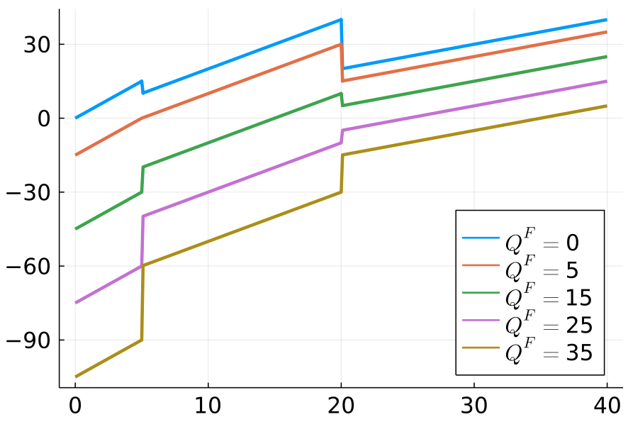
Figure 1: Revenue curves, $\tilde{\Lambda}(e,\omega)$, for various values of $Q^{F}$.

Finally, we remark that in both [10] and [11], the revenue function is not stochastic since it only considers thermal bids in the form of thermal installed capacities and operating costs and does not require the Markovian SDDP. In this setting, we allow stochastic and time-dependent energy bids from other agents. The more general framework of this work requires the usage of Markovian SDDP, just like in the price taker case with spot price uncertainty [5].

IV Multiple agents

In this section, we combine the methodologies presented in the previous sections to describe a novel simulation algorithm that approximates the interaction among multiple price-maker and price-taker agents. All the interactions between agents will be in terms of price and quantity bid offers as in a realistic competitive energy market.

First, we note that we can obtain an initial hint on the bids of multiple agents from a simulation of the centralized audited-cost-based market design of the power system through the typical cost-minimization SDDP. As described in Section II, the results of a simulation of the power system include primal and dual variable solutions for each $t$ and $s$. By collecting the generation decisions of all units of a generation agent $i$, at a given stage $t$ and scenario $s$, we have the quantity part of the bid. Collecting the simulated marginal operating costs for $t$ and $s$, we can define (within the audited-cost-based market design) the spot prices of the system ($\mathit{\Pi}=\{\pi_{s,t}\}_{t\in T,s\in S}$) as well as a hint for the price parcel of the bids to initialized the equilibrium search algorithm. Therefore, we denote the set of price and quantity bids of an agent $i$ as $(\mathcal{P}_{i},\mathcal{Q}_{i})=\{P_{i,t,s},Q_{i,t,s}\}_{t\in T,s\in S}$, which means that there is one pair of price and quantity for each sampled scenario $s\in S$ and stage $t\in T$. We will name the procedure of solving a cost-minimization long-term dispatch problem with audited costs and obtaining both spot prices $\mathit{\Pi}$ and bids for all agents $(\mathcal{P},\mathcal{Q})$ as $CentralizedOperation(\mathcal{A},\mathcal{R})$. The inputs $(\mathcal{A},\mathcal{R})$ represent scenarios of inflows and renewable maximum generation, which are samples of the random variables for all stages. Because bids and spot prices, $(\mathcal{P},\mathcal{Q},\mathit{\Pi})$, are obtained from a procedure that relies on correlated inflows and renewable generation scenarios, $(\mathcal{A},\mathcal{R})$, these random variables must be jointly simulated [40].

The self-optimization of price taker agents requires spot prices of the system, as described in Section III, see (19), (10)–(16). On the other hand, strategic agents require bids from all other agents as described in Section III with the revenue function (24). Price and quantity bids from other agents and spot prices are time-dependent random variables. Therefore, solving this multi-stage stochastic problem will require the Markovian SDDP to handle the time dependency of random variables in the objective function (see [5, 41]). We can estimate a Markov Chain based on inflows, renewable generation, spot price, and bid data, $(\mathcal{A},\mathcal{R},\mathit{\Pi},\mathcal{P},\mathcal{Q})$ that are all the random variables associated to the strategic agent optimization. The estimation of the Markov chain results in transition probabilities $M^{t}_{\mu|m}$ between the Markov states $\mu$ and $m$ for each stage $t$. The collection of transition probabilities, $M^{t}_{\mu|m}$, between all Markov states for all stages, $t\in T$, will be denoted as $\mathcal{M}$. This process that takes the tuple $(\mathcal{A},\mathcal{R},\mathit{\Pi},\mathcal{P},\mathcal{Q})$ and returns $\mathcal{M}$, will be denoted as $EstimateMarkovChain(\mathcal{A},\mathcal{R},\mathit{\Pi},\mathcal{P},\mathcal{Q})$.

The strategic optimization of an agent $i$, as a function of the inflows $\mathcal{A}$, renewable generation $\mathcal{R}$, bids of other agents $(\mathcal{P}_{-i},\mathcal{Q}_{-i})$, and Markov transition probabilities $\mathcal{M}$, is labeled $StrategicBid(\mathcal{A},\mathcal{R},\mathcal{P}_{-i},\mathcal{Q}_{-i},\mathcal{M})$ and relies on the solution of (30)–(31). Similarly, we define the price-taker optimization of agent $i$ as $PriceTakerBid(\mathcal{A},\mathcal{R},\mathcal{P}_{-i},\mathcal{Q}_{-i},\mathcal{M})$, which relies on the solution of (17)–(18), (19). Analogous to the simulation step of $CentralizedOperation(\mathcal{A},\mathcal{R})$, both $StrategicBid(\cdot)$ and $PriceTakerBid(\cdot)$ return an updated bid, $(\mathcal{P}_{i},\mathcal{Q}_{i})$, for the optimized agent $i$. The quantity part of the bid are the primal solutions of the energy offer $e$, whereas prices are obtained by computing the respective spot price in (20)–(23). Thus, we can obtain updated spot prices, $\mathit{\Pi}$, by clearing the market for each stage and scenario given bids from all agents, $(\mathcal{P},\mathcal{Q})$. We label this procedure as $ClearMarket(\mathcal{P},\mathcal{Q})$.

The complete simulation algorithm is based on the diagonalization method extensively used in the literature of competitive hydro-power markets [19, 26, 27, 24, 28]. We will resort to the above-defined procedures to initialize and then iteratively update the bids of one price maker agent at a time while the bids from other agents are fixed. The process stops when changes in those bids are within some given tolerance. The main goal is to simulate the power market in an agent-based fashion. If convergence is strictly attained, we might have reached a Nash equilibrium. However, such an equilibrium might not even exist in this setting.

Algorithm 1 depicts the proposed method. The algorithm starts by computing bids, $(\mathcal{P},\mathcal{Q})$, for all price taker and price maker agents with the $CentralizedOperation(\mathcal{A},\mathcal{R})$ procedure. Then, a first estimate of the Markov process is made with the $EstimateMarkovChain(\mathcal{A},\mathcal{R},\mathit{\Pi},\mathcal{P},\mathcal{Q})$ procedure. After that, there will be a loop through all the price taker $i\in I^{T}$ and price maker $i\in I^{M}$. For each agent $i$, new bids, $(\mathcal{P}_{i},\mathcal{Q}_{i})$, are obtained from the $StrategicBid(\mathcal{A},\mathcal{R},\mathcal{P}_{-i},\mathcal{Q}_{-i},\mathcal{M})$ or the $PriceTakerBid(\mathcal{A},\mathcal{R},\mathcal{P}_{-i},\mathcal{Q}_{-i},\mathcal{M})$ procedures. Then, spot prices and the Markov process estimation are updated by the $ClearMarket(\mathcal{P},\mathcal{Q})$ and $EstimateMarkovChain(\mathcal{A},\mathcal{R},\mathit{\Pi},\mathcal{P},\mathcal{Q})$ routines. Finally, if some convergence criterion is attained, the algorithm stops. Otherwise, it continues to a new round of bid updates. The convergence criterion considered in this work is assuring the maximum absolute variation of the price and quantity bids of all agents vary less than a given small number: 1% of their values in the centralized operation.

Algorithm 1 Multiple Agent Simulation

  

  $(\mathcal{P},\mathcal{Q},\mathit{\Pi})\leftarrow CentralizedOperation(\mathcal{A},\mathcal{R})$

  $\mathcal{M}\leftarrow EstimateMarkovChain(\mathcal{A},\mathcal{R},\mathcal{P},\mathcal{Q},\mathit{\Pi})$

  while no convergence do

     for $i\in I^{T}$ do

        $(\mathcal{P}_{i},\mathcal{Q}_{i})\leftarrow PriceTakerBid(\mathcal{A},\mathcal{R},\mathcal{P}_{-i},\mathcal{Q}_{-i},\mathcal{M})$

     end for

     for $i\in I^{M}$ do

        $(\mathcal{P}_{i},\mathcal{Q}_{i})\leftarrow StrategicBid(\mathcal{A},\mathcal{R},\mathcal{P}_{-i},\mathcal{Q}_{-i},\mathcal{M})$

     end for

     $\mathit{\Pi}\leftarrow ClearMarket(\mathcal{P},\mathcal{Q})$

     $\mathcal{M}\leftarrow EstimateMarkovChain(\mathcal{A},\mathcal{R},\mathcal{P},\mathcal{Q},\mathit{\Pi})$

  end while

V Computational Experiments with The Brazilian Southeastern System

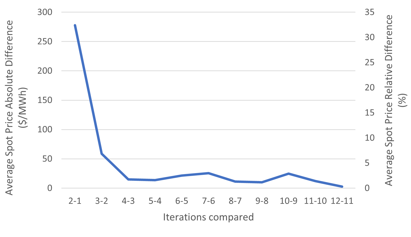
Figure 2: Convergence profile from Brazil’s southeast with $(25\%,50\%)$ and no contracts. See Figure 3a. Average spot price absolute and relative differences between two consecutive iterations: $(i+1)$–$(i)$.

In this section, we provide quantitative simulated results for the Brazilian power system. We begin with a sensitivity analysis based on the Brazilian Southeast subsystem, which accounts for about $55\%$ of the Brazilian hydro resources and about $50\%$ of the system’s total installed capacity. We analyze different market concentration and contracting schemes based on the procedure developed in Section IV.

V-A Dataset, infrastructure, and system configuration

This system was constructed from real data from the Brazilian system expansion scenario for $2025$ and contains $46$ thermal plants and $21$ hydro plants with a simplified topology of the system. Note that this is already more than the current $13$ aggregated reservoirs considered in the official model. The overall hydro generation installed capacity represents $70\%$ of the system’s installed capacity. To illustrate the algorithm’s functioning, first, we consider three main hydro generation companies, one considered as a price taker agent, and the other two as price makers. The $21$ hydro plants are split into $3$ aforementioned groups of generation companies. All thermal plants are considered individual price-taker agents. We considered a single load block for the sake of simplicity. The following simulations were carried out in a $5$-year monthly horizon, that is, $60$ stages. We considered $1000$ sampled scenarios. The large-scale simulations were performed in a PSRCloud cluster of $8$ servers, each one with $64$ cores and $128$GB of RAM. Each simulation took approximately $3$ hours. All algorithms were coded in the Julia language [42], and the optimization models were coded with JuMP [43] and solved with the Xpress solver[44].

V-B Impact of Market Concentration on Market Power

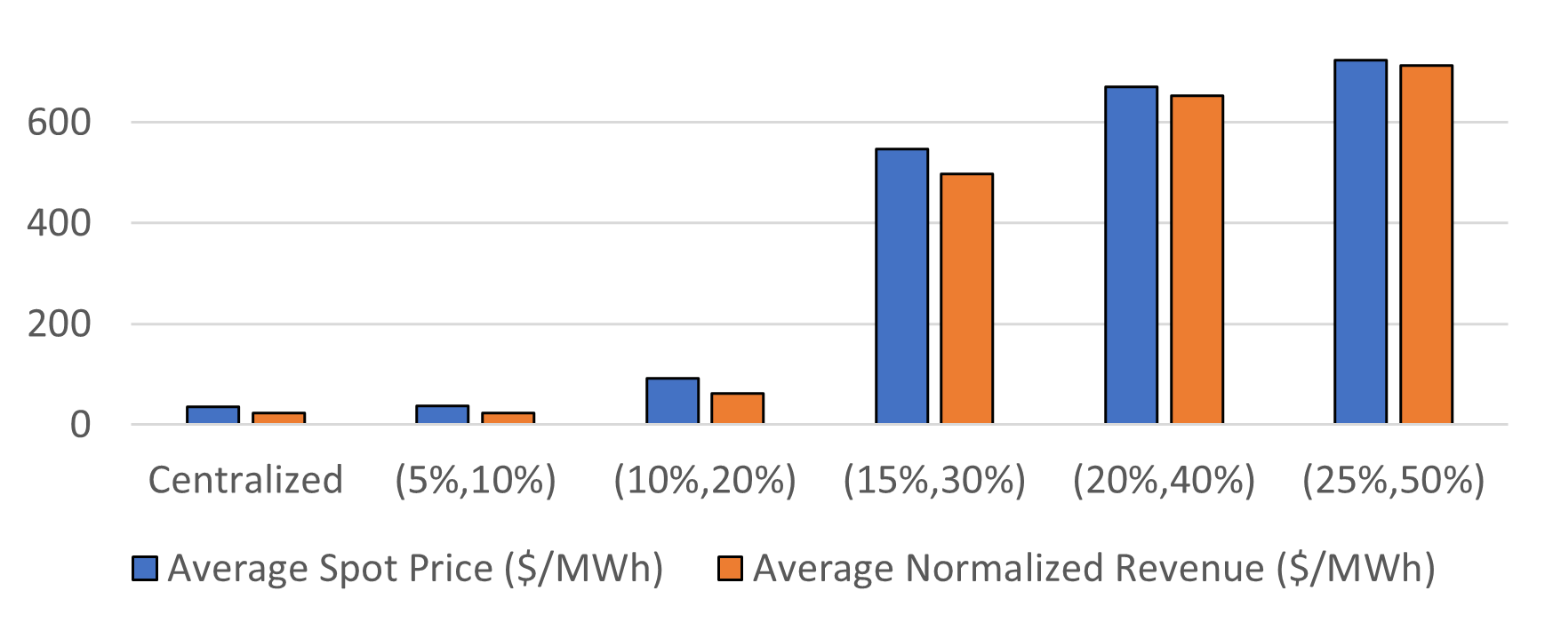
(a)

(b)

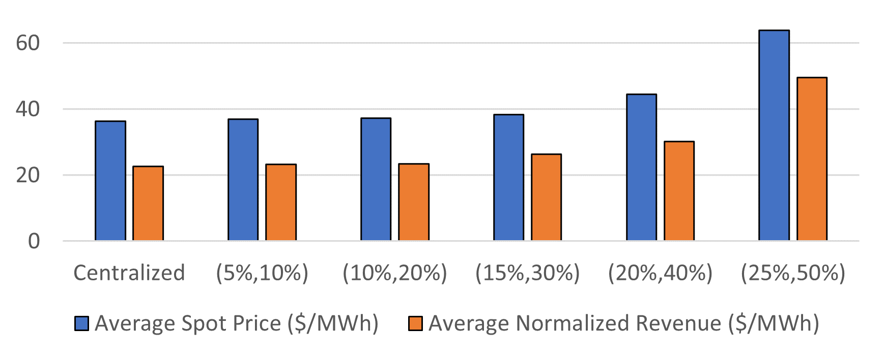
(c)

(d)

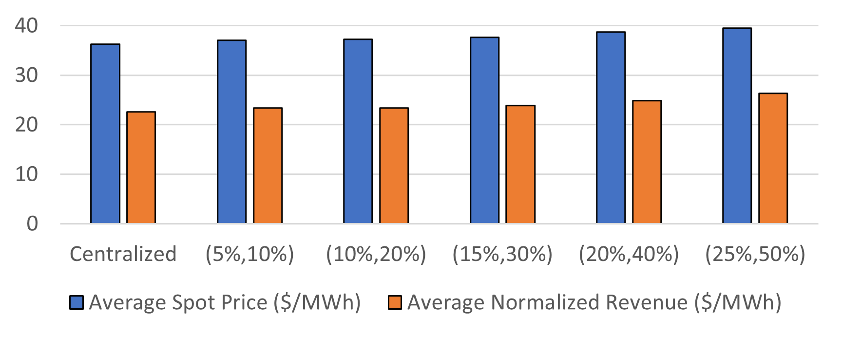
(e)

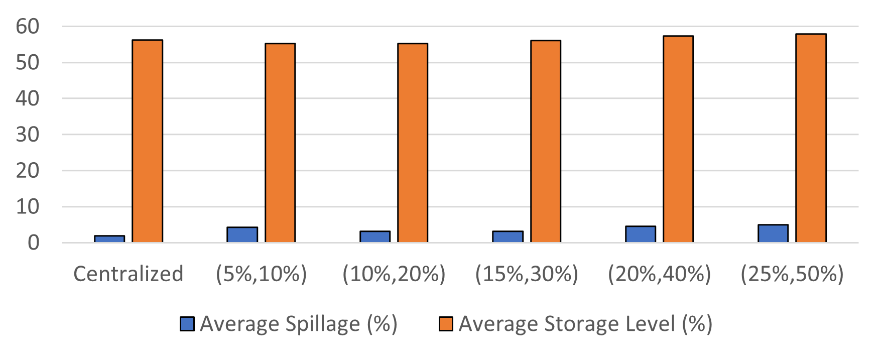
(f)

Figure 3: Results for simulations of Brazil’s Southeast under different market concentrations. (a) and (b) no contracts, (c) and (d) $75\%$ of contracting level, (e) and (f) $100\%$ of contracting level. In parentheses in the horizontal axis, we have the percent share of each price maker agent. Average values of Spot Prices, Normalized Revenue, Spillage, and Storage Level are with respect to all stages and scenarios. Spillage and Storage $\%$ are with respect to the maximum amount of water that can be stored in the system.

In this section, we present five controlled simulation experiments to understand the effect of different market concentrations on market power abuse. We adjust the hydro plants so that we have different databases defined by tuples $({share}_{1}\%,{share}_{2}\%)$. In each case, ${share}_{1}$ and ${share}_{2}$ represent the shares (in percentage) of the hydro system belonging to each of the two price maker companies (agents). The remainder of the hydro system is assumed to be of price-taker agents.

Figure 2 presents a typical convergence profile of the proposed iterative method. These profiles were taken from the case study with price maker shares of $(25\%,50\%)$ and no contracts. Figure 2 shows both average absolute and relative differences between two consecutive iterations. First, absolute (or relative) differences are computed for each stage and scenario, and then, they are averaged.

In Figure 3a, we show the average spot prices as a function of the market distributions in a bar plot. We add the first bar with the spot price of the centralized dispatch. As expected, the spot prices rapidly grow as the concentration increases. The Figure also depicts the captured price, i.e., the average value of energy sold, which is the total revenue of each agent divided by its total generated energy. We present results in such normalized forms so that we can compare the results of different-sized agents. Figure 3b shows additional results with average reservoir levels of the price maker agents throughout the study period and the average spillage. Interestingly, market power abuse is mostly characterized by excess spillage, whereas, on average, the total reservoir levels are mostly kept unchanged compared to the benchmark (centralized dispatch with audited costs).

V-C Impact of Contracts on Market Power

In this section, we repeat the above analyses but with contracts. To come up with monthly contract quantities, we take average generation values from the centralized dispatch and prices from the average spot prices in the centralized dispatch. This will stimulate the agents to produce energy and reduce the spot prices since being short in the contract together with high spot prices will lead the agent to have expenses due to the second term in (32).

Figures 3c, 3d, 3e and 3f contain the same metrics presented in the previous section but for the cases of agents that are $75\%$ and $100\%$ contracted, respectively. In the case studies, we can clearly see that the contracts completely eradicated the market power, and the resulting spot prices are very close to the ones obtained in the centralized dispatch. At the same time, the captured revenues and spillage levels were shrunk to values close to the ones observed on the centralized dispatch with audited costs. By analyzing Figures 3d and 3b (price makers $0\%$ and $75\%$ contracted), we can see that spillage is a relevant marker for market power abuse.

VI Case Study: The Brazilian Power System

In this section, we provide results for a case study considering the complete Brazilian power system. We contrast results from simulations with and without contracts and provide a first quantitative measurement of the market power abuse potential in this system.

VI-A Dataset, infrastructure, and system configuration

This dataset was created from the original data of the Brazilian system and contains $137$ thermal plants representing $18\%$ of the installed capacity, $364$ renewable energy plants (wind and solar) representing $19\%$ of the installed capacity and $32$ hydropower plants representing the remaining $63\%$ of the installed capacity. Here, we improve the load duration curve accuracy and consider $5$ load blocks instead of just one to consider peak demand hours. Like in previous studies, we consider $5$ years ($60$ monthly stages), $1000$ scenarios, and the same PSRCloud cluster configuration.

In this study, we consider an approximation of the real market concentration in the system. We represent three companies as price maker agents, with respectively $32\%$, $9\%$ and $7\%$ of the energy resources representing the three largest generation owners. Meanwhile, the remaining $55\%$ of the generators are distributed among one price-taker hydro company, and each thermoelectric generator is considered another small price-taker agent. Each simulation took approximately $11$ hours.

VI-B Market Power in the Brazilian Power System as a Function of the Contracting Level

First, we simulated the centralized operation and the bid-based market without contracts. Then, we considered agents with multiple contracting levels in the bid-based market. In particular, we analysed the cases of: $25\%$, $50\%$, $75\%$ and $100\%$ of contracting level. The key results from each of the $6$ simulations are depicted in Figures 4 and 5.

Figure 4 shows the spot price under the above $6$ conditions. We can see the progression from the case with the highest spot prices, where no contracts are considered, until the fully contracted case, where the average spot price is much closer to the one obtained from the centralized operation with audited costs. Given the number of resources allocated to the price maker agents, $45\%$, we note that a $75\%$ contracting level effectively reduces the gap to the centralized operation. This closely follows what we have seen in the previous section with the southeastern system. In such case, $75\%$ was also effective in containing market power in the case where the first price-maker agent had $15\%$ and the second price maker had $30\%$ of the resources resulting in a $45\%$ share of the system in the hands of price-maker agents. Finally, we note that even low contracting levels, such as $25\%$, significantly reduce the final average spot prices. So, we highlight the empirical evidence depicted in our case study that the typical contracting levels observed in practice, ranging from $75\%$ to $100\%$, can be seen as a relevant instrument to prevent market power abuse in the Brazilian power system.

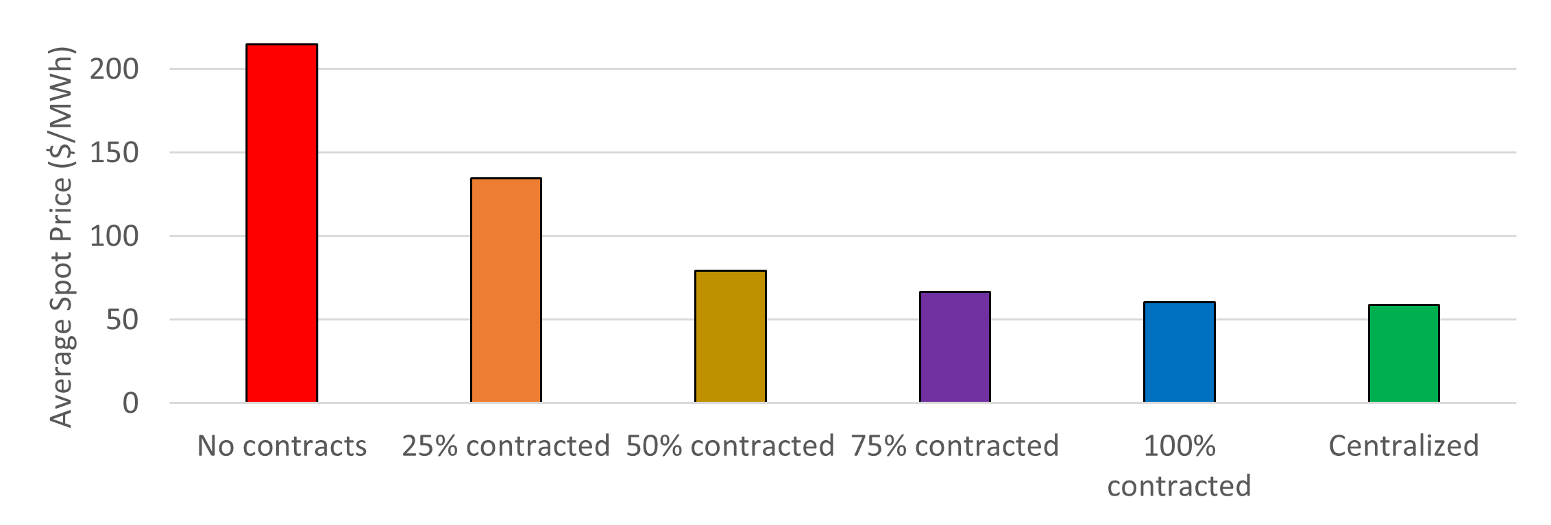
Figure 4: Average Spot Price ($/MWh) for the Brazilian system under different contracting levels. Averages with respect to stages and scenarios.

Figure 5 presents the overall revenue, including operation and contract costs and spot and contract revenue throughout the $5$-year horizon for each of the three price-maker agents. Overall, the figure reproduces information already verified in Figure 4 with excessive revenues for all agents for the bid-based cases with no contracts. Notably, the $100\%$ contracting case leads to revenues that are very similar to the ones from the centralized dispatch. Again, $75\%$ seems to be a relevant threshold value as it induces revenues and spot prices relatively close to the ones obtained in the centralized case.

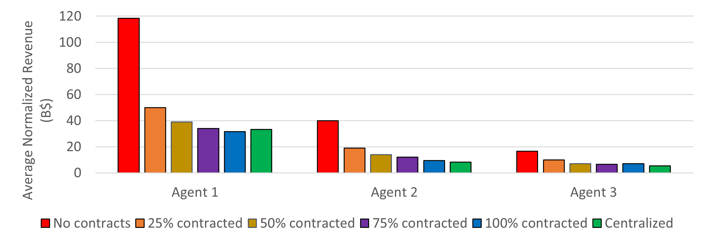
Figure 5: Average normalized revenue ($/MWh) for each of the $3$ price maker agents under different contracting levels. Averages with respect to stages and scenarios.

VII Conclusion

Based on relevant works on long-term hydrothermal power markets, we combined three key pieces to develop a new and effective market simulator, namely: 1) SDDP applied to the centralized hydrothermal dispatch to initialize and benchmark the process, 2) a multistage bilevel stochastic model for strategic bidding of a single-player to obtain decisions from price maker agents, and 3) an iterative diagonalization-based method to simulate the interactions among agents in the market. In contrast to the existing literature on the subject, with our new algorithm, we could jointly consider multiple reservoirs (32), multiple stages (60) and scenarios (1,000), and multiple price-maker agents (3). Therefore, a realistic large-scale case study based on the Brazilian power system (one of the largest in the world) could be addressed, and relevant insights could be obtained.

Within the limitations of the presented computational experiments and case study, which include all assumptions of the proposed model and the specific data, the results and analyses carried out in this work allow us to convey the following concluding remarks for the Brazilian power system:

1. We found evidence that the market concentrations observed in the current Brazilian electricity market are capable of enabling market power abuse.

2. The spillage level is a relevant market for market power abuse.

3. Contracts are relevant instruments to prevent market power abuse in this country.

4. A $75\%$ contracting level, typically observed in Brazilian hydro generation companies, is effective in reducing market power abuse.

We highlight that the developed market analysis tool can help regulators and market/system operators in market monitoring activities, expansion studies, and understanding the impact of new market rules and instruments. On the algorithmic side, the method is suitable for parallel computing and can be extended to consider other physical and regulatory details. Finally, we showcase that a real-world problem formulated as a multistage bilevel stochastic problem can be solved under reasonable assumptions and provide relevant insights to decision-makers and regulators.

References

- [1] IEA, “Hydropower,” https://www.iea.org/reports/hydropower, June 2022.
- [2] M. V. F. Pereira and L. M. V. G. Pinto, “Multi-stage stochastic optimization applied to energy planning,” Mathematical Programming, vol. 52, no. 1-3, pp. 359–375, 1991.
- [3] “Conversations on designs – wholesale electricity markets,” IEEE Power and Energy Magazine, vol. 17, pp. 1–108, January 2019.
- [4] L. Ribeiro, A. Street, D. Valladão, A. C. Freire, and L. Barroso, “Technical and economical aspects of wholesale electricity markets: An international comparison and main contributions for improvements in brazil,” Electric Power Systems Research, vol. 220, p. 109364, 2023.
- [5] A. Gjelsvik, M. M. Belsnes, and A. Haugstad, “An algorithm for stochastic medium-term hydrothermal scheduling under spot price uncertainty,” in Proceedings of 13th Power Systems Computation Conference, 1999.
- [6] N. Löhndorf and A. Shapiro, “Modeling time-dependent randomness in stochastic dual dynamic programming,” European Journal of Operational Research, vol. 273, no. 2, pp. 650–661, 2019.
- [7] G. Steeger, L. A. Barroso, and S. Rebennack, “Optimal bidding strategies for hydro-electric producers: A literature survey,” Power Systems, IEEE Transactions on, vol. 29, no. 4, pp. 1758–1766, 2014.
- [8] G. Gross and D. Finlay, “Generation supply bidding in perfectly competitive electricity markets,” Computational & Mathematical Organization Theory, vol. 6, no. 1, pp. 83–98, 2000.
- [9] D. Pozo, E. Sauma, and J. Contreras, “Basic theoretical foundations and insights on bilevel models and their applications to power systems,” Annals of Operations Research, vol. 254, no. 1-2, pp. 303–334, 2017.
- [10] B. Flach, L. Barroso, and M. Pereira, “Long-term optimal allocation of hydro generation for a price-maker company in a competitive market: latest developments and a stochastic dual dynamic programming approach,” IET generation, transmission & distribution, vol. 4, no. 2, pp. 299–314, 2010.
- [11] G. Steeger and S. Rebennack, “Dynamic convexification within nested Benders decomposition using Lagrangian relaxation: An application to the strategic bidding problem,” European Journal of Operational Research, vol. 257, no. 2, pp. 669–686, 2017.
- [12] M. Habibian, A. Downward, and G. Zakeri, “Multistage stochastic demand-side management for price-making major consumers of electricity in a co-optimized energy and reserve market,” European Journal of Operational Research, vol. 280, no. 2, pp. 671–688, 2020.
- [13] J. I. Pérez-Díaz, I. Guisández, M. Chazarra, and A. Helseth, “Medium-term scheduling of a hydropower plant participating as a price-maker in the automatic frequency restoration reserve market,” Electric Power Systems Research, vol. 185, p. 106399, 2020.
- [14] J. Arteaga and H. Zareipour, “A Price-Maker/Price-Taker Model for the Operation of Battery Storage Systems in Electricity Markets,” IEEE Transactions on Smart Grid, vol. 10, no. 6, pp. 6912–6920, 2019.
- [15] L. A. Barroso, R. D. Carneiro, S. Granville, M. V. Pereira, and M. Fampa, “Nash equilibrium in strategic bidding: a binary expansion approach,” Power Systems, IEEE Transactions on, vol. 21, no. 2, p. 629, 2006.
- [16] B. Fanzeres, A. Street, and D. Pozo, “A column-and-constraint generation algorithm to find nash equilibrium in pool-based electricity markets,” Electric Power Systems Research, vol. 189, p. 106806, 2020.
- [17] T. J. Scott and E. G. Read, “Modelling hydro reservoir operation in a deregulated electricity market,” International Transactions in Operational Research, vol. 3, no. 3-4, pp. 243–253, 1996.
- [18] R. Kelman, L. A. N. Barroso, and M. V. F. Pereira, “Market power assessment and mitigation in hydrothermal systems,” Power Systems, IEEE Transactions on, vol. 16, no. 3, pp. 354–359, 2001.
- [19] J. Villar and H. Rudnick, “Hydrothermal market simulator using game theory: assessment of market power,” Power Systems, IEEE Transactions on, vol. 18, no. 1, pp. 91–98, 2003.
- [20] J. P. Molina, J. M. Zolezzi, J. Contreras, H. Rudnick, and M. J. Reveco, “Nash-cournot equilibria in hydrothermal electricity markets,” IEEE Transactions on Power Systems, vol. 26, no. 3, pp. 1089–1101, 2010.
- [21] H. Höschle, H. Le Cadre, Y. Smeers, A. Papavasiliou, and R. Belmans, “An admm-based method for computing risk-averse equilibrium in capacity markets,” IEEE Transactions on Power Systems, vol. 33, no. 5, pp. 4819–4830, 2018.
- [22] G. Steeger and S. Rebennack, “Strategic bidding for multiple price-maker hydroelectric producers,” IIE Transactions, vol. 47, no. 9, pp. 1013–1031, 2015.
- [23] M. Löschenbrand, W. Wei, and F. Liu, “Hydro-thermal power market equilibrium with price-making hydropower producers,” Energy, vol. 164, pp. 377–389, 2018.
- [24] X. Wu, C. Cheng, S. Miao, G. Li, and S. Li, “Long-Term Market Competition Analysis for Hydropower Stations using SSDP-Games,” Journal of Water Resources Planning and Management, vol. 146, no. 6, p. 04020037, 2020.
- [25] J. Bushnell, “A Mixed Complementarity Model of Hydrothermal Electricity Competition in the Western United States,” Operations Research, vol. 51, no. 1, pp. 80–93, 2003. 7 stages cal+PAC but no limit.
- [26] K. C. Almeida and A. J. Conejo, “Medium-Term Power Dispatch in Predominantly Hydro Systems: An Equilibrium Approach,” IEEE Transactions on Power Systems, vol. 28, no. 3, pp. 2384–2394, 2013.
- [27] M. Cruz, E. Finardi, V. d. Matos, and J. Luna, “Strategic bidding for price-maker producers in predominantly hydroelectric systems,” Electric Power Systems Research, vol. 140, pp. 435–444, 2016.
- [28] Y. Liang, Q. Lin, S. He, Q. Liu, Z. Chen, and X. Liu, “Power Market Equilibrium Analysis with Large-scale Hydropower System Under Uncertainty,” 2020 IEEE PES Innovative Smart Grid Technologies Europe (ISGT-Europe), vol. 00, pp. 329–333, 2020.
- [29] E. Moiseeva and M. R. Hesamzadeh, “Bayesian and Robust Nash Equilibria in Hydrodominated Systems Under Uncertainty,” IEEE Transactions on Sustainable Energy, vol. 9, no. 2, pp. 818–830, 2018.
- [30] G. Infanger and D. P. Morton, “Cut sharing for multistage stochastic linear programs with interstage dependency,” Mathematical Programming, vol. 75, no. 2, pp. 241–256, 1996.
- [31] A. Shapiro, “Analysis of stochastic dual dynamic programming method,” European Journal of Operational Research, vol. 209, no. 1, pp. 63–72, 2011.
- [32] A. Shapiro, W. Tekaya, J. P. da Costa, and M. P. Soares, “Risk neutral and risk averse stochastic dual dynamic programming method,” European journal of operational research, vol. 224, no. 2, pp. 375–391, 2013.
- [33] B. Rudloff, A. Street, and D. M. Valladão, “Time consistency and risk averse dynamic decision models: Definition, interpretation and practical consequences,” European Journal of Operational Research, vol. 234, no. 3, pp. 743–750, 2014.
- [34] A. W. Rosemberg, A. Street, J. D. Garcia, D. M. Valladão, T. Silva, and O. Dowson, “Assessing the cost of network simplifications in long-term hydrothermal dispatch planning models,” IEEE Transactions on Sustainable Energy, vol. 13, no. 1, pp. 196–206, 2021.
- [35] S. Debia, P.-O. Pineau, and A. S. Siddiqui, “Strategic storage use in a hydro-thermal power system with carbon constraints,” Energy Economics, vol. 98, p. 105261, 2021.
- [36] G. L. M. Fredo, E. C. Finardi, and V. L. de Matos, “Assessing solution quality and computational performance in the long-term generation scheduling problem considering different hydro production function approaches,” Renewable energy, vol. 131, pp. 45–54, 2019.
- [37] P. Lino, L. A. N. Barroso, M. V. Pereira, R. Kelman, and M. H. Fampa, “Bid-based dispatch of hydrothermal systems in competitive markets,” Annals of Operations Research, vol. 120, no. 1-4, pp. 81–97, 2003.
- [38] L. Barroso, S. Granville, P. Jackson, M. Pereira, and E. Read, “Overview of virtual models for reservoir management in competitive markets,” in Proceedings 4th IEEE/Cigré International Workshop on Hydro Scheduling in Competitive Markets, Bergen, Norway, 2012.
- [39] J. Zou, S. Ahmed, and X. A. Sun, “Stochastic dual dynamic integer programming,” Mathematical Programming, vol. 175, no. 1-2, pp. 461–502, 2019.
- [40] J. A. Dias, G. Machado, A. Soares, and J. D. Garcia, “Modeling multiscale variable renewable energy and inflow scenarios in very large regions with nonparametric bayesian networks,” arXiv preprint arXiv:2003.04855, 2020.
- [41] T. Silva, D. Valladão, and T. Homem-de Mello, “A data-driven approach for a class of stochastic dynamic optimization problems,” Computational Optimization and Applications, vol. 80, pp. 687–729, 2021.
- [42] J. Bezanson, A. Edelman, S. Karpinski, and V. B. Shah, “Julia: A fresh approach to numerical computing,” SIAM review, vol. 59, no. 1, pp. 65–98, 2017.
- [43] M. Lubin, O. Dowson, J. Dias Garcia, J. Huchette, B. Legat, and J. P. Vielma, “JuMP 1.0: Recent improvements to a modeling language for mathematical optimization,” Mathematical Programming Computation, vol. 15, p. 581–589, 2023.
- [44] FICO, “FICO Xpress Optimizer Reference Manual,” 2023.