An Exactly Solvable Model for Single-Lane Unidirectional Ant Traffic

Abstract

In 2002, Chowdhury et al. introduced a simplified model aimed at depicting the dynamics of single-lane unidirectional ant traffic. Despite efforts, an exact solution for the stationary state of this ant-trail model remains elusive. The primary challenge arises from inherent fluctuations in the total amount of pheromone along the ant-trail. These fluctuations significantly influence ant movement. Consequently, unlike conventional models involving driven interacting particles, the average velocity exhibits non-monotonic behavior with ant density. In this study, we propose an exactly solvable model for ant traffic whose dynamics is based on the one in Chowdhury et al.’s model, and then discuss the circumstances under which the non-monotonic trend of average velocity arises.

• March 2024

Keywords: Ant-Trail Model, Exactly Solvable Model, Exclusion Process.

1 Introduction

Insects use various ways to communicate, including visual signals, sounds, and chemicals. Pheromones, in particular, play a crucial role in communication among species insects. For example, ants use trail pheromones to guide colony members to food sources and back to the nest. The study of these insect colonies has contributed to various fields such as computer science [10], communication engineering [6], artificial intelligence [11], micro-robotics [20], as well as task partitioning and decentralized manufacturing [1, 2, 3, 27, 28].

To investigate the collective movements of ants along already established paths, researchers have used different models to understand how ants move in groups. One such model, introduced by Chowdhury et al. [8], as referenced in [29], has been particularly useful. It helps study how ants move along paths and how they interact with each other. A generation of this model can be found in [15]. Couzin and Franks [9] developed an individual-based model, which not only accounts for the emergence of self-organized lanes but also offers insights into variations in ant flux. Moreover, a continuous model was proposed in [18]. The present study will focus specifically on the Chowdhury et al.’s model, as its dynamics are interdependent with ours.

In regular traffic, vehicles decelerate as more cars fill the road, leading to congestion (see Subsection 1.1). In contrast, the Chowdhury et al.’s model of unidirectional ant traffic (Subsection 1.2) reveals a non-monotonic trend due to the interaction of ants’ dynamics with pheromones.

1.1 Totally asymmetric simple exclusion process

In 1970, Spitzer proposed a mathematical model for exclusion process inspirited from biological traffic concerns [23, 24]. It serves as a toy model in nonequilibrium statistical physics to investigate nonequilibrium phenomena and phase transitions induced by boundaries. Recent literature on this subject is available in [7, 29]. For a more comprehensive understanding of the process, readers can consult [19, 22, 23, 30, 31, 32].

The exclusion process is a continuous-time Markov chain, wherein random particles must obey the exclusion principle, ensuring they do not occupy the same position simultaneously. Furthermore, particles are allowed to move from one lattice site to an adjacent site only if the destination site is unoccupied. On the lattice, we denote a vacant site by 0 and a site occupied by a particle by 1. This study focuses exclusively on variations of the one-dimensional Totally Asymmetric Simple Exclusion Process (TASEP), characterized by the following simple dynamics

$$10\to 01\text{ with rate }1.$$ (1)

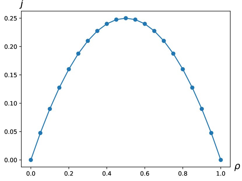
(a) Average current $j$

(b) Average velocity $\nu$

Figure 1: The average particle current $j$ and velocity $\nu$ of TASEP vary as functions of density $\rho$. The current exhibits symmetry, and the velocity $\nu$ decreases linearly with density $\rho$.

In a lattice with periodic boundary conditions, the stationary distribution of the TASEP is uniform. In the thermodynamic limit, the stationary particle velocity $\nu$ and current $j$ are determined as functions of the particle density $\rho$, as follows

$$\nu=1-\rho,\ \ j=\rho(1-\rho).$$ (2)

Fig. 1 illustrates that the stationary current of particles demonstrates symmetry, while the stationary velocity follows a monotone decreasing pattern. Additionally, in the steady state particle distribution, correlations are notably absent. These characteristics contrast with findings in biological traffic models, as studied by [4, 8, 12, 13], where particle interactions on the same lattice tend to be cooperative. Furthermore, these features are also not observed in the model proposed by Chowdhury et al. [8] for ants movement along established trail, as discussed in next subsection.

1.2 Chowdhury et al.’s model

The unidirectional ant-traffic model (ATM) proposed by Chowdhury et al. [8] extends the concept of the TASEP. In this model, the motion of ants is coupled with a secondary field representing the presence or absence of pheromones (see Fig. 2). Specifically, the probability of ants hopping is now influenced by the detection of pheromones at the destination site, leading to a higher probability of movement. Additionally, the dynamics of the pheromones are defined: they are produced by ants, and free pheromones evaporate with a probability of $f$ per unit of time. The model comprises two stages: in Stage I, ants are allowed to move, while in Stage II, pheromones are permitted to evaporate. The authors implement parallel updates for the dynamics in each stage, meaning that stochastic dynamic rules are simultaneously applied for all ants and pheromones, independently.

In the one-dimensional ATM, each site represents a cell capable of hosting one ant at most. These lattice sites are indexed as $i$ ($i=1,2,...,L$), with $L$ denoting the lattice’s length. At each site $i$, one associates two binary variables, $A_{i}$ and $P_{i}$. The variable $A_{i}$ takes a value of 0 or 1, indicating whether the cell is vacant or occupied by an ant, respectively. Similarly, $P_{i}=1$ signifies the presence of pheromone in cell $i$, while $P_{i}=0$ indicates its absence. Thus, the model encompasses two sets of dynamic variables: $A(t)\equiv(A_{1}(t),A_{2}(t),...,A_{i}(t),...,A_{L}(t))$ and $P(t)\equiv(P_{1}(t),P_{2}(t),...,P_{i}(t),...,P_{L}(t))$. The complete state, or configuration, of the system at any given time $t$ is fully described by the combined set $\{A(t),P(t)\}$. Before restating the dynamics of Chowdhury et al.’s model, for later convenience, we assume ants only move leftward.

Stage I: Motion of ants. In this stage, all ants are allowed to move simultaneously following the assigned probabilities. When there are no neighboring ants to the left, the probability of an ant’s forward movement (to the left as previously assumed) is either $q$ or $Q$, depending on whether the target site contains pheromones. Here, $q$ represents the average speed of an ant without pheromones directly ahead of the ant, while $Q$ represents the speed with pheromones at the neighboring site to the left. Considering the configuration of the system $\{A,P\}$, let us assume an ant is located at site $i$, represented as $A_{i}(t)=1$. The rates of the ant’s movement to site $i-1$ can be expressed as

$$\begin{cases}01\to 10\text{ with rate }q\text{ if }P_{i-1}(t)=0,\\ 01\to 10\text{ with rate }Q\text{ if }P_{i-1}(t)=1.\end{cases}$$ (3)

Stage II: Evaporation of pheromones. This stage follows Stage I. Cells where ants have left retain pheromones. Additionally, pheromones on sites without ants are free to evaporate. This evaporation is considered a random process happening at an average rate of $f$ per unit of time. Thus, given at time $t$, there is pheromone at site $i$, i.e., $P_{i}(t)=1$, one has

$$\begin{cases}P_{i}(t+1)=0\text{ with rate }f,\\ P_{i}(t+1)=1\text{ with rate }1-f.\end{cases}$$ (4)

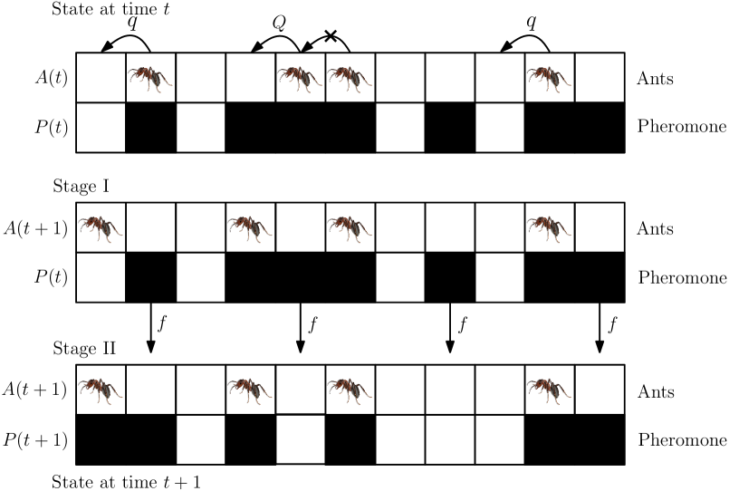
Figure 2: Illustration depicting typical configurations and the update process. At the top of the figure, it shows a configuration at time $t$ before stage I of the update, along with the possibility of ants jumping with assigned probabilities. In the middle, the configuration after one potential realization of stage I is shown, where two ants move to the left while others remain unmoved. Additionally, in the middle of the figure, it also depicts the pheromones that may evaporate during stage II of the update scheme. At the bottom, one potential configuration after the realization of stage II is shown, indicating the evaporation of two pheromones and the creation of one pheromone due to ant motion.

As noted earlier, ant movement incorporates the presence of trail pheromones, leading to a non-monotonic behavior in the average velocity of ants for small values of $f$. Referring to Figs. 2 and 3 in [8] illustrates this phenomenon. This contrasts with the behavior observed in the TASEP and other vehicular traffic models, where inter-vehicle interactions impede motion, resulting in a monotonic decrease in average vehicle speed with increasing density. Additional sources supporting the model can be found in [16, 17] and [29].

1.3 Motivations and Organization

As noted in [4, 29], an exact solution for Chowdhury et al.’s model remains elusive. In response to this challenge, two approximate theories have been proposed. The first utilizes a mean-field approach [8, 25]. However, this method encounters limitations in the intermediate density regime, where dynamics are governed by loose clusters that cannot be accurately represented by mean-field theories assuming a uniform distribution of ants. The second approach involves mapping the system onto a zero-range process (ZRP) [21, 25], as the model’s dynamics closely resemble those of a ZRP. This mapping, akin to the procedure in TASEP, identifies particles (ants) with the sites of the ZRP, while the gaps between the ants correspond to the particles of the ZRP [14, 26].

The challenge lies in performing an exact analysis of ATM due to fluctuations in the total amount of pheromones on the ant-trail. Fortunately, a model proposed by Belitsky and Schütz for the RNA Polymerase [4, 5] explains the collective pushing phenomenon of traffic in biology and successfully captures fluctuations of this kind. In this work, we modify the model to suit our specific setting.

The remainder of the paper is structured as follows: Section 2 introduces the dynamics and stationary distribution of the model, presenting the main result, Theorem 2.1. The proof of this result is detailed in Appendix A. In Section 3, we analyze the average current and velocity of ants. Following this analysis, Section 4 delves into a discussion of these quantities. Finally, we give conclusions in Section 5.

2 Ant-trail model with random-sequential update

As the same in Chowdhury et al. model [8], instead of exploring the emergence of ant trails, our focus is on observing ant traffic along an already established trail. Unlike the model, which employs parallel dynamics, our model utilizes a random-sequential update rule.

Our approach is the following. Initially, we propose dynamics of the ATM on a one-dimensional envisioned lattice with a length of $L$, where individual lattice sites are sequentially numbered from 1 to $L$. We assume that ants cannot overlap, and there exists an interaction between these ants, akin to the behavior observed in the TASEP for particles. However, our goal is to establish a more complex interaction rule, leading to emergent behaviors beyond what the TASEP can demonstrate. These interactions are defined by explicit formulas for the transition rates. We propose that the stationary distribution of our model adheres to a specific form. Finally, we determine the constraints on parameters in the transition rates to ensure that the envisioned distribution indeed represents the stationary distribution for the dynamics specified by those rates.

2.1 The model state space and dynamics

We begin this subsection by introducing the types of particles. In our context, cells on the ant trail that are occupied by ants are considered as empty sites. Thus, a site occupied by an ant is designated as state 0, representing an empty location. A site without any ant but containing pheromone is denoted as state 2, while an unoccupied site (totally empty) is labeled as state 1. It is important to emphasize that in this context, ant motion aligns with the movement of empty sites. Moreover, each jump made by particle 0 (ant) corresponds to a jump made by particle 1 (empty cell) or 2 (cell with pheromone but without the presence of an ant). Therefore, to analyze ant movement, one can study the motion of particle types 1 and 2.

In typical behavior, we assume that particles of both types 1 and 2 move to the right, while empty sites (representing ants) shift to the left. With the particle type notations in mind, instead of employing parallel updates as in the model by Chowdhury et al. (illustrated in Fig. 2), we modify the dynamics of our model using random-sequential updates. The dynamics of ants corresponding to Chowdhury et al.’s model in the Stage I and the evaporation of pheromones in the Stage II are now simply expressed as

$$\begin{cases}10\to 02,\ \ &\text{with rate }q^{\star},\\ 20\to 02,\ \ &\text{with rate }Q^{\star},\\ 2\to 1,\ \ &\text{with rate }f^{\star}.\end{cases}$$ (5)

In this context, the parameters $q^{\star}$, $Q^{\star}$, and $f^{\star}$ serve the same purposes as $q$, $Q$, and $f$ respectively. To maintain consistency with observed ant trails, we presume $q^{\star}$ to be less than $Q^{\star}$, as the presence of pheromones typically boosts the average speed of ants.

Before delving into the dynamics of ants and pheromones, let us establish the state space of our model. Given our focus on the collective movement of ants, we will assume periodic boundary conditions, where the lattice $\mathbb{T}_{L}$ comprises $L$ sites, with $i+L\equiv i\mod L$. Considering that there are $L-N$ ants on this lattice, where $N$ represents the total number of particles of types 1 and 2, we represent a system configuration as $\boldsymbol{\eta}=(\eta_{1},\ldots,\eta_{L})$, where $\eta_{j}\in\{0,1,2\}$ for $j=1,2,\ldots,L$, signifying an allowed arrangement of particles.

It is evident that the transition rates depend on the surrounding environment, specifically the presence of pheromones and ants. Thus, in our context, the transition rates of a particle are contingent upon the current positions of ants and pheromones. Consequently, the rates $q^{\star}$, $Q^{\star}$, and $f^{\star}$ rely on the current configuration. Thus, given a configuration $\boldsymbol{\eta}$, the transition rates of each particle can be different since each depends on its surrounding environment. To emphasize this dependence, we denote the transition rates of the $i$-th particle as $q_{i}(\boldsymbol{\eta})$, $Q_{i}(\boldsymbol{\eta})$, and $f_{i}(\boldsymbol{\eta})$. Refer to Fig. 3 for an illustration of the dynamics involving a single particle for both types.

Figure 3: Minimal reaction scheme of particle translocation. Particle can move from site $i$ to site $i+1$ provided it is in state 1 (empty cell) and change its state to 2 (cell with pheromone but without any ant located on it) with an effect rate $q_{i}(\boldsymbol{\eta})$. Similarly, if the particle is in state 2 at site $i$, it can move to site $i+1$ with a rate of $Q_{i}(\boldsymbol{\eta})$, maintaining its state. Additionally, at site $i$, a particle in state 2 can change to state 1 without moving indicating pheromone fade away, and this transition occurs with a rate of $f_{i}(\boldsymbol{\eta})$.

Note that that an allowed configuration $\boldsymbol{\eta}=(\eta_{1},...,\eta_{L})$ can be defined using both a position vector $\textbf{x}=(x_{1},...,x_{N})$ and a state vector $\textbf{s}=(s_{1},...,s_{N})$ for the particles. Here, $x_{i}$ represents the coordinate of the $i$-th particle on the lattice, which is calculated modulo $L$, while $s_{i}$ represents the state of this particle, belonging to $\{1,2\}$. It is important to note that $x_{i}$ denotes the position of particle $i$, rather than representing the position of an ant. The advantage of employing the position vector lies in its ability to express the distance between two particles using the Kronecker-$\delta$ function, defined as follows

$$\delta_{u,v}=\begin{cases}1,&\text{if }u=v,\\ 0,&\text{if }u\neq v,\end{cases}$$ (6)

for any $u,v$ belonging to any set.

Assumption: Pairs of ants located at neighboring sites enhance the translocation rates. This assumption is quite natural, as the leading ant leaves a pheromone trail on the path, resulting in it attracting the ant right behind to move faster.

Now we are in a position to state the rates influenced by the surrounding environment. Consider the $i$-th particle, which undergoes a rightward jump with rates $q_{i}(\boldsymbol{\eta})$ and $Q_{i}(\boldsymbol{\eta})$, depending on whether its state is 1 or 2, respectively. Moreover, if its state is 2, there exists an additional possibility for transitioning to state 1 due to evaporating pheromone, governed by the rate $f_{i}(\boldsymbol{\eta})$. The rates of the models described above are given by

$$q_{i}(\boldsymbol{\eta}) =\delta_{s_{i},1}q^{\star}(1+\delta_{x_{i}+2,x_{i+1}}q^{\star 01})(1-\delta_{x_{i}+1,x_{i+1}}),$$ (7)

$$Q_{i}(\boldsymbol{\eta}) =\delta_{s_{i},2}Q^{\star}(1+\delta_{x_{i}+2,x_{i+1}}Q^{\star 01})(1-\delta_{x_{i}+1,x_{i+1}}),$$ (8)

$$f_{i}(\boldsymbol{\eta}) =\delta_{s_{i},2}f^{\star}(1+\delta_{x_{i-1},x_{i}-1}f^{1\star}+\delta_{x_{i}+1,x_{i+1}}f^{\star 1}+\delta_{x_{i-1},x_{i}-2}f^{10\star}+\delta_{x_{i}+2,x_{i+1}}f^{\star 01}).$$ (9)

To ensure that the rates remain positive, certain conditions must be met: $q^{\star 01},Q^{\star 01}>-1$; $f^{\star 1},f^{1\star},f^{\star 01},f^{10\star}>-1$; $f^{\star 1}+f^{10\star},f^{1\star}+f^{\star 01}>-1$ . In equations (7) and (8), the term $(1-\delta_{x_{i}+1,x_{i+1}})$ indicates that the effectiveness of the jump rates $q_{i}(\boldsymbol{\eta})$ and $Q_{i}(\boldsymbol{\eta})$ depends on whether the next right site of particle $i$ is unoccupied. This term is equal to 0 when the $i$-th and $(i+1)$-th particles are located neighboring sites. Regarding the superscripts, the symbol $\star$ indicates the position of particle $i$, alongside the symbol 0 representing an unoccupied site and the symbol 1 representing an occupied site. Thus, $q^{\star 01}$ and $Q^{\star 01}$ represent the contribution to $q_{i}(\boldsymbol{\eta})$ and $Q_{i}(\boldsymbol{\eta})$ when the $i$-th particle is positioned one empty site away from particle $(i+1)$. The condition of a distance of 1 between the two particles is specified by the term $\delta_{x_{i}+2,x_{i+1}}$, which equals to 1 only when the two particles are separated by a distance of 1. Refer to Figs. 4 and 5 for examples of the rates $q_{i}(\boldsymbol{\boldsymbol{\eta}})$ and $Q_{i}(\boldsymbol{\boldsymbol{\eta}})$. The role of parameters $q^{\star 01}$ and $Q^{\star 01}$ is discussed below. Similarly, the contributions of parameters $f^{1\star}$, $f^{\star 1}$, $f^{10\star}$, and $f^{\star 01}$ to the rate $f_{i}(\boldsymbol{\eta})$ can be explained. For example, the value $f^{\star 1}$ is added to the rate when there is a particle at site $x_{i}+1$, as indicated by the term $\delta_{x_{i}+1,x_{i+1}}$. See Fig. 6 for some examples of the rate $f_{i}(\boldsymbol{\boldsymbol{\eta}})$.

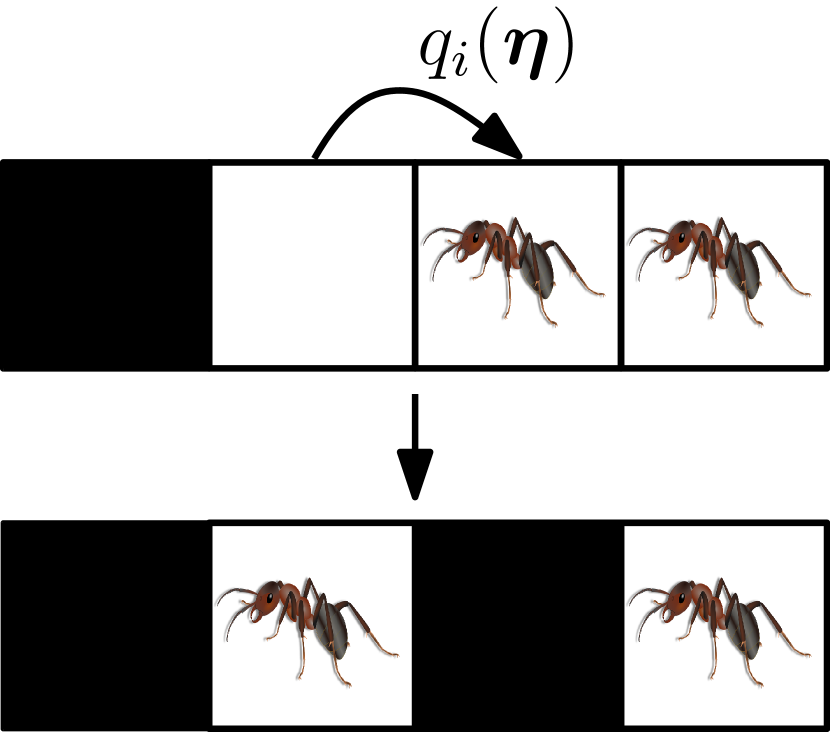
(a) $q_{i}(\boldsymbol{\eta})=q^{\star}$

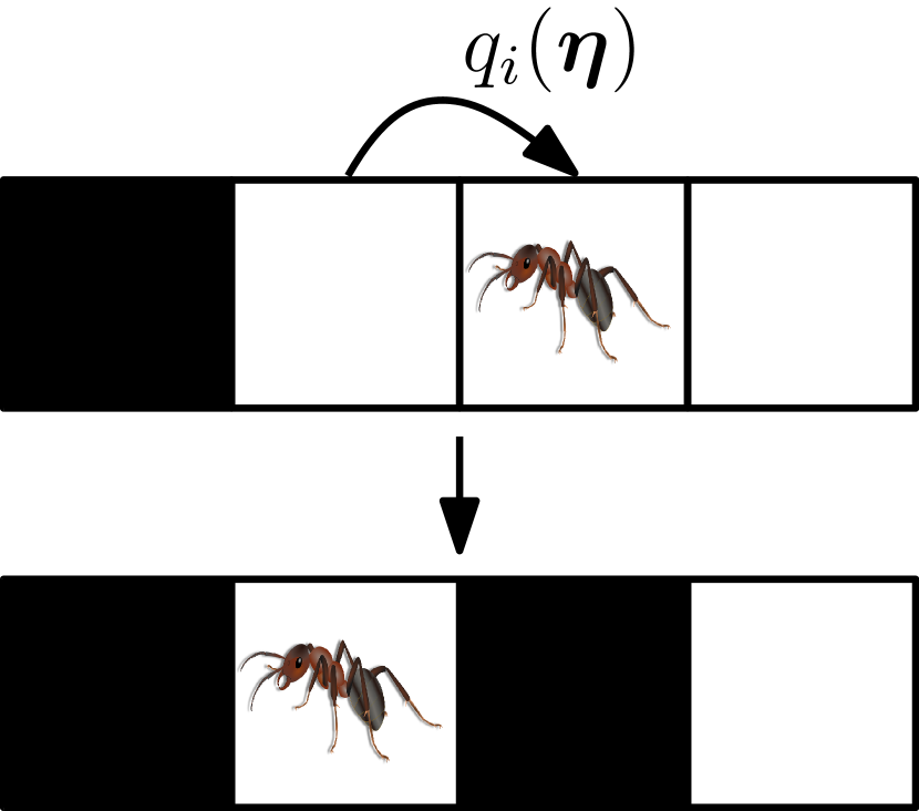
(b) $q_{i}(\boldsymbol{\eta})=q^{\star}(1+q^{\star 01})$

Figure 4: Here are a few illustrations of the translocation rate $q_{i}(\boldsymbol{\eta})$ for a particle in state 1. In these visual representations, empty cells indicate that the particles are in state 1, while filled cells represent state 2. Cells with ants are considered empty sites.

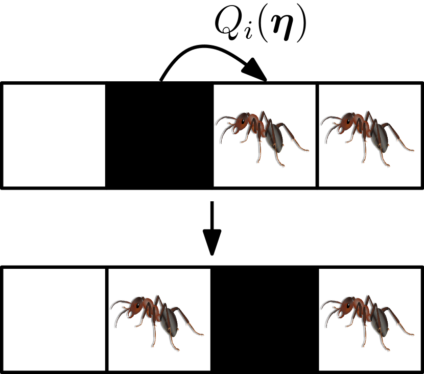
(a) $Q_{i}(\boldsymbol{\eta})=Q^{\star}$

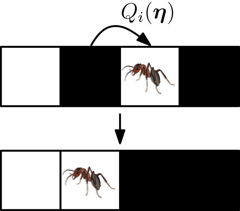
(b) $Q_{i}(\boldsymbol{\eta})=Q^{\star}(1+Q^{\star 01})$

Figure 5: Here are a few illustrations of the translocation rate $Q_{i}(\boldsymbol{\eta})$ for a particle in state 1. In these visual representations, empty cells indicate that the particles are in state 1, while filled cells represent state 2. Cells with ants are considered empty sites.

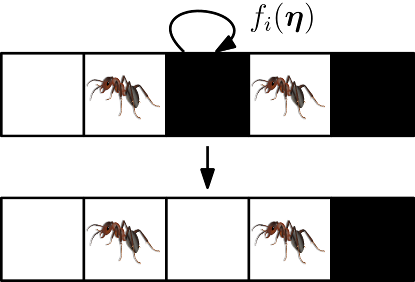
(a) $f_{i}(\boldsymbol{\eta})=f^{\star}(1+f^{10\star}+f^{\star 01})$

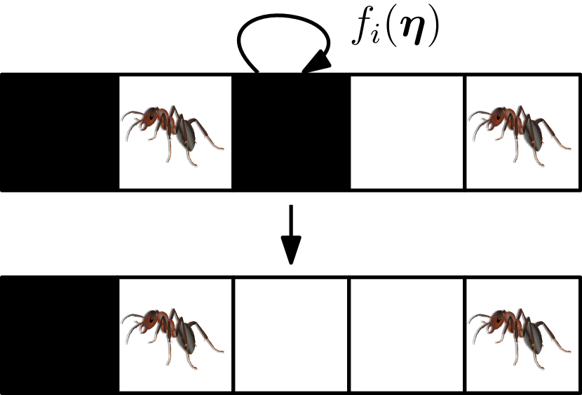
(b) $f_{i}(\boldsymbol{\eta})=f^{\star}(1+f^{10\star}+f^{\star 1})$

Figure 6: Here are a few illustrations of the translocation rate $f_{i}(\boldsymbol{\eta})$ for a particle in state 1. In these visual representations, empty cells indicate that the particles are in state 1, while filled cells represent state 2. Cells with ants are considered empty sites.

Neighboring-effect parameters: Let us clarify the role of the parameter $q^{\star 01}$ using Fig. 4 as an illustration. In Fig. 4(a), we observe a scenario where two ants are positioned at neighboring sites, resulting in a jump rate of the particle with state 1 being $q(\boldsymbol{\boldsymbol{\eta}})=q^{\star}$. However, when there are no ants in proximity, as shown in Fig. 4(b), the rate becomes $q(\boldsymbol{\boldsymbol{\eta}})=q^{\star}(1+q^{\star 01})$. Therefore, selecting $q^{\star 01}<0$ indicates that the latter rate is lower than the former, suggesting that pairs of ants enhance the rates. The role of $Q^{\star 01}$ mirrors that of $q^{\star 01}$. Hence, we designate both parameters $q^{\star 01}$ and $Q^{\star 01}$ as neighboring-effect parameters, given their influence on the rates at which ants locate neighboring sites.

2.2 The model stationary distribution

Let $\boldsymbol{\eta}$ denote a system configuration, defined by position vectors $\textbf{x}=(x_{1},...,x_{N})$ and state vectors $\textbf{s}=(s_{1},...,s_{N})$. In addition to the hardcore repulsion, as discussed in [4], we include a short-range interaction energy term in the Hamiltonian, expressed as

$$U(x)=J\sum_{i=1}^{N}\delta_{x_{i}+1,x_{i+1}}$$ (10)

Here, a positive $J$ indicates repulsion among the particles, whereas it signifies attraction among the ants. Note that the sum $\sum_{i=1}^{N}\delta_{x_{i}+1,x_{i+1}}$ counts the number of pairs of particles located on neighboring sites.

We use $N^{\alpha}$ to represent the fluctuating number of particles in state $\alpha\in\{1,2\}$, where $N=N^{1}+N^{2}$. Additionally, we define the excess as $B(\textbf{s})=N^{1}-N^{2}$. Therefore, the stationary measure is defined as

$$\pi(\boldsymbol{\eta})=\dfrac{1}{Z}e^{-\frac{1}{k_{B}T}(U(x)+\lambda B(s))}.$$ (11)

Here, $Z$ denotes the partition function, defined as $Z=\sum_{\boldsymbol{\eta}}\pi(\boldsymbol{\eta})$. The chemical potential $\lambda$ acts as a Lagrange multiplier to account for fluctuations in the difference between the number of particles in states 1 and 2, referred to as the excess

$$B(\textbf{s})=\sum_{i=1}^{N}(3-2s_{i}).$$ (12)

These fluctuations arise from the interaction between the retention of ant pheromones on the trail and their gradual degradation over time. $k_{B}$ is the Boltzmann constant and $T$ plays a role as temperature.

To facilitate future computational tasks, we introduce

$$x=e^{\frac{2\lambda}{k_{B}T}}\text{ and }y=e^{\frac{J}{k_{B}T}},$$ (13)

so that $x>1$ corresponds to an excess of particle in state 1 and repulsive interaction corresponds to $y>1$. Thus, the stationary distribution (11) becomes

$$\pi(\boldsymbol{\eta})=\dfrac{1}{Z}\prod_{i=1}^{N}x^{3/2-s_{i}}y^{-\delta_{x_{i}+1,x_{i+1}}}.$$ (14)

Note that the dynamics (7)–(9) and stationary measure (14) of the model are described in parameter form. Parameters cannot be arbitrarily chosen to ensure that the process, governed by the dynamics, possesses a measure in the form of (11) as its invariant distribution. Namely, the model’s parameters must conform to the following constraints:

$$x =\dfrac{q^{\star}}{f^{\text{$\star$}}},$$ (15)

$$y =\dfrac{1+\dfrac{1}{f^{\star}}Q^{\star}}{1+q^{\star 01}+\dfrac{1}{f^{\star}}Q^{\star}(1+Q^{\star 01})},$$ (16)

$$f^{1\star} =\dfrac{x}{1+x}-\dfrac{x}{1+x}\dfrac{Q^{\star}}{q^{\star}}-1,$$ (17)

$$f^{\star 1} =\dfrac{1}{1+x}+\dfrac{x}{1+x}\dfrac{Q^{\star}}{q^{\star}}-1,$$ (18)

$$f^{10\star} =\dfrac{1}{1+x}(1+q^{\star 01})+\dfrac{x}{1+x}\dfrac{Q^{\star}}{q^{\star}}(1+Q^{\star 01})-\dfrac{1}{1+x}-\dfrac{x}{1+x}\dfrac{Q^{\star}}{q^{\star}},$$ (19)

$$f^{\star 01} =\dfrac{x}{1+x}(1+q^{\star 01})-\dfrac{x}{1+x}\dfrac{Q^{\star}}{q^{\star}}(1+Q^{\star 01})-\dfrac{x}{1+x}+\dfrac{x}{1+x}\dfrac{Q^{\star}}{q^{\star}}.$$ (20)

In other words, one can summarize the results by Theorem 2.1 below. The proof of this theorem can be found in Appendix A.

Theorem 2.1

If the parameters specified in rates (7)–(9) satisfy the conditions outlined in (15)–(20), the invariant measure of the process is given by

$$\hat{\pi}(\boldsymbol{\eta})=\dfrac{1}{Z}\left(\dfrac{q^{\star}}{f^{\text{$\star$}}}\right)^{\sum_{i=1}^{N}-3/2+s_{i}}\left(\dfrac{1+\dfrac{1}{f^{\star}}Q^{\star}}{1+q^{\star 01}+\dfrac{1}{f^{\star}}Q^{\star}(1+Q^{\star 01})}\right)^{-\sum_{i=1}^{N}\delta_{x_{i+1},x_{i}+1}}$$ (21)

where $Z$ denotes the partition function.

Remark 2.1

The parameters $q^{\star}$, $Q^{\star}$, $f^{\star}$, $q^{\star 01}$, and $Q^{\star 01}$ play a crucial role in the dynamics of the model, as the other parameters can be expressed through them.

3 Average current and velocity

In this section, we calculate the average current and velocity of ants. Before doing so, we compute certain quantities such as the average stationary densities and the average dwell times of particles in the two states. These calculations are helpful in computing the average current and velocity.

3.1 Average dwell times and stationary densities

Average excess: As highlighted in [4], the most straightforward measure for defining particle distribution is the average excess density of type 1 over type 2, represented as

$$\sigma=\dfrac{\left<N^{1}\right>-\left<N^{2}\right>}{L}.$$ (22)

Because we use the grand-canonical ensemble (66), which is of the same form as the one in [4], we similarly obtain the value $\sigma$ as follows

$$\sigma=\dfrac{1-x}{1+x}\rho_{p}.$$ (23)

where $\rho_{p}$ is the particle density, i.e., $\rho_{p}=N/L$. However, the difference in the value of $\sigma$ compared to the one stated in the paper arises from the value $x$, as our model’s dynamics are not the same as those in the paper.

Average densities: We denote by

$$\rho^{\alpha}:=\left<\delta_{s_{i},\alpha}\right>=\dfrac{1}{L}\left<N^{\alpha}\right>,\ \ \alpha\in\{1,2\},$$ (24)

the average densities of particle in states $1$ and $2$. Since $\rho^{1}+\rho^{2}=\rho_{p}$ and using (23), we obtain

$$\rho^{1}=\dfrac{1}{1+x}\rho_{p},\ \ \rho^{2}=\dfrac{x}{1+x}\rho_{p}.$$ (25)

Average dwell times: Let $\tau^{\alpha}$, where $\alpha\in\{1,2\}$, denote the average dwell time that a particle spends in states 1 and 2, respectively. Due to ergodicity, we have $\tau^{\alpha}=\rho^{\alpha}/\rho_{p}$. This yields the following formulas for average dwell times

$$\tau^{1}=\dfrac{1}{1+x},\ \ \tau^{2}=\dfrac{x}{1+x}.$$ (26)

From equations (25) and (26), we derive the balance equation

$$\dfrac{\rho^{1}}{\rho^{2}}=\dfrac{\tau^{1}}{\tau^{2}}=\dfrac{f^{\star}}{q^{\star}}.$$ (27)

This equation expresses the ensemble ratio in relation to the single-particle translocation rates $q^{\star}$ and the single-particle transition rate $f^{\star}$.

3.2 Average stationary current and velocity

As previously noted, we analyze the collective movement of ants by studying the motion of particles governed by dynamics (7)–(9). The current $j_{p}$, quantified as the average number of particles traversing a site per unit time, reflects the collective motion of these particles. Additionally, the average speed $\nu_{p}$ of particles is another characteristic of collective movement, which is linked to $j_{p}$ through the equation

$$j_{p}=\rho_{p}\nu_{p}.$$ (28)

Instead of using the form of rates (7)–(8) to compute $j_{p}$ and $\nu_{p}$, it is equivalent to use the rates in headway form (42)–(43) for convenience. The advantage is that it incorporates the headway distribution (72) into the computation. Namely, one has

$$j_{p}=\langle\delta_{s_{i},1}(q^{\star}(1+q^{\star 01})\theta_{i}^{1}+q^{\star}\theta_{i}^{>1})\rangle+\langle\delta_{s_{i},2}(Q^{\star}(1+Q^{\star 01})\theta_{i}^{1}+Q^{\star}\theta_{i}^{>1})\rangle.$$ (29)

Here, $\langle\cdot\rangle$ indicates taking the expectation with respect to the distribution (66), and the headway variable $\theta_{i}^{>1}$ indicates that there are more than one empty site ahead of particle $i$, i.e., $x_{i+1}-x_{i}>2$. By utilizing the factorization property of the grandcanonical ensemble (66) and the identities in (25), one obtains

$$j_{p} =\langle\delta_{s_{i},1}\rangle\langle(q^{\star}(1+q^{\star 01})\theta_{i}^{1}+q^{\star}\theta_{i}^{>1})\rangle+\langle\delta_{s_{i},2}\rangle\langle(Q^{\star}(1+Q^{\star 01})\theta_{i}^{1}+Q^{\star}\theta_{i}^{>1})\rangle$$

$$=\dfrac{1}{1+x}\rho_{p}\big{(}q^{\star}(1+q^{\star 01})\langle\theta_{i}^{1}\rangle+q^{\star}\langle\theta_{i}^{>1}\rangle\big{)}+\dfrac{x}{1+x}\rho_{p}\big{(}Q^{\star}(1+Q^{\star 01})\langle\theta_{i}^{1}\rangle+Q^{\star}\langle\theta_{i}^{>1}\rangle\big{)}.$$ (30)

From headway distribution (72), one can compute $\langle\theta_{i}^{0}\rangle,\langle\theta_{i}^{1}\rangle$ and one has

$$\langle\theta_{i}^{>1}\rangle=1-\langle\theta_{i}^{0}\rangle-\langle\theta_{i}^{1}\rangle.$$ (31)

From this point, we have sufficient ingredients to draw graphs showing the average current and velocity of ants. However, notice that the average current $j$ and velocity $v$ of ants with density $\rho=1-\rho_{p}$ are related to $j_{p}$ and $\nu_{p}$ as follows

$$\begin{cases}j(\rho)=j_{p}(1-\rho_{p}),\\ v(\rho)=j(\rho)/\rho.\end{cases}$$ (32)

The influence of neighboring-effect parameters $q^{\star 01},Q^{\star 01}$, and evaporating rate $f^{\star}$ on average current and velocity of ants is examined. Two scenarios are considered: when $Q^{\star 01}\leq q^{\star 01}$ and when $Q^{\star 01}\geq q^{\star 01}$. Refer to Figs. 7, 8, 9, 10, 11, 12, 13, 14, 15, 16, 17 and 18 for the former case, and Figs. 19 and 20 for the latter. In the following graphs, as previously mentioned, we select the values of $Q^{\star}$ and $q^{\star}$ such that $Q^{\star}>q^{\star}$, indicating that the rate with pheromone at the destination site exceeds the rate without pheromone at the site. Namely, in all the graphs presented below, the values of $Q^{\star}$ and $q^{\star}$ are set to 1 and 0.25, respectively.

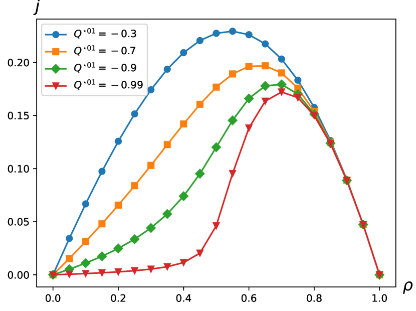
(a) Average current $j$

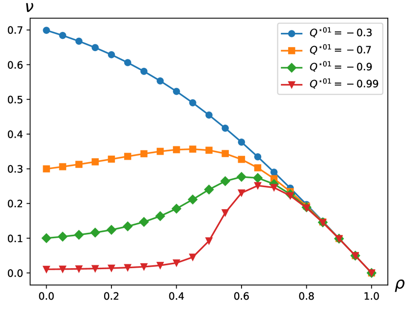
(b) Average velocity $\nu$

Figure 7: Average current $j$ and velocity $\nu$ as functions of ant density $\rho$. $Q^{\star}=1,q^{\star}=0.25,q^{\star 01}=-0.2,f^{\star}=0.0005$ with different values of $Q^{\star 01}=-0.3;-0.7;-0.9;-0.99$.

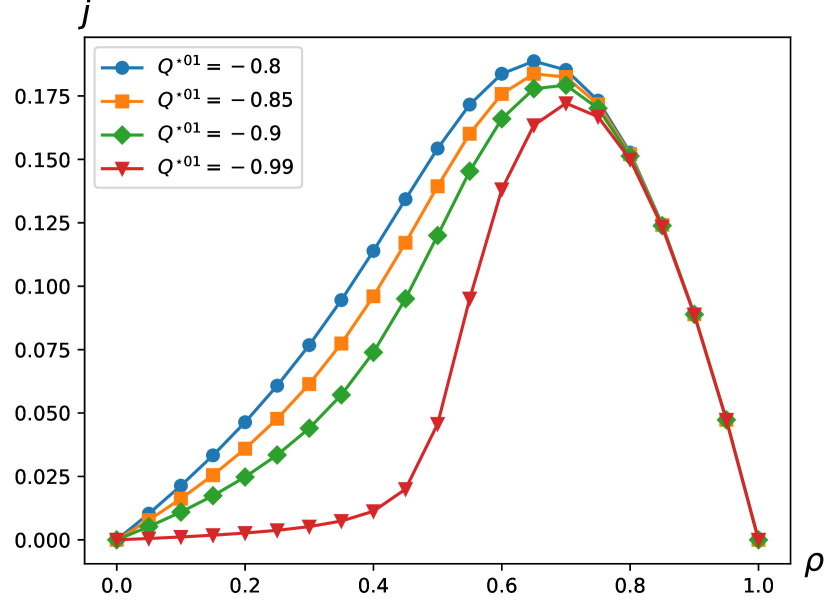
(a) Average current $j$

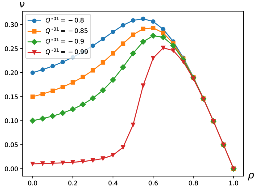
(b) Average velocity $\nu$

Figure 8: Average current $j$ and velocity $\nu$ as functions of ant density $\rho$. $Q^{\star}=1,q^{\star}=0.25,q^{\star 01}=-0.7,f^{\star}=0.0005$ with different values of $Q^{\star 01}=-0.8;-0.85;-0.9;-0.99$.

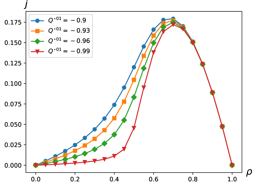
(a) Average current $j$

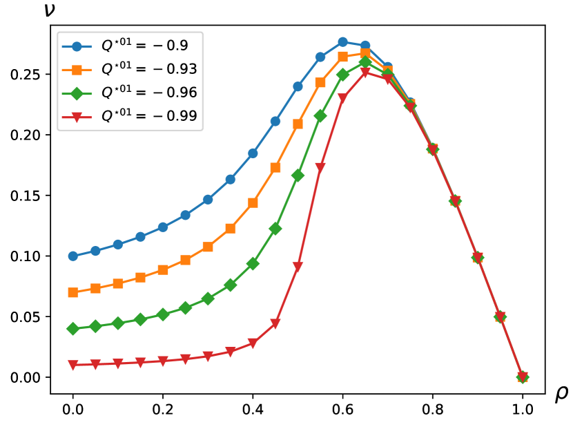
(b) Average velocity $\nu$

Figure 9: Average current $j$ and velocity $\nu$ as functions of ant density $\rho$. $Q^{\star}=1,q^{\star}=0.25,q^{\star 01}=-0.9,f^{\star}=0.0005$ with different values of $Q^{\star 01}=-0.9;-0.93;-0.96;-0.99$.

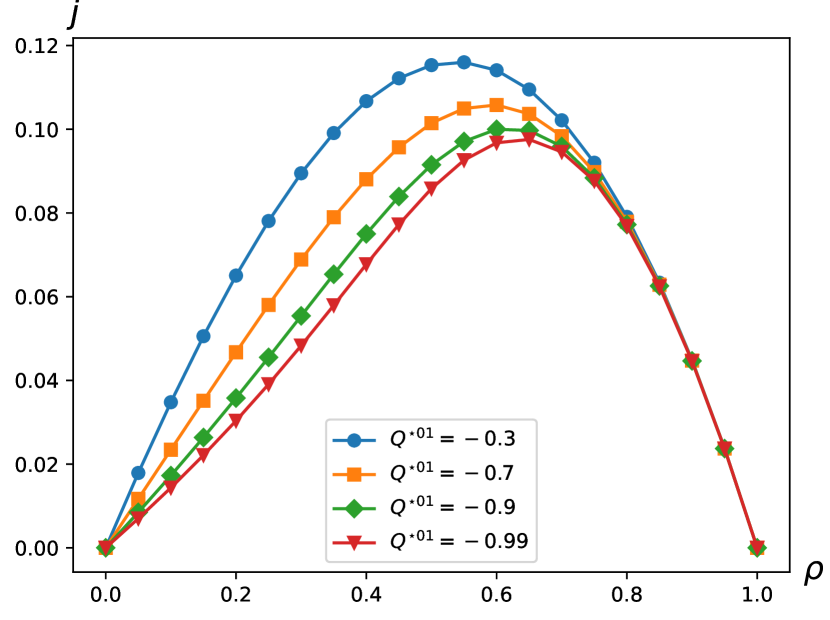
(a) Average current $j$

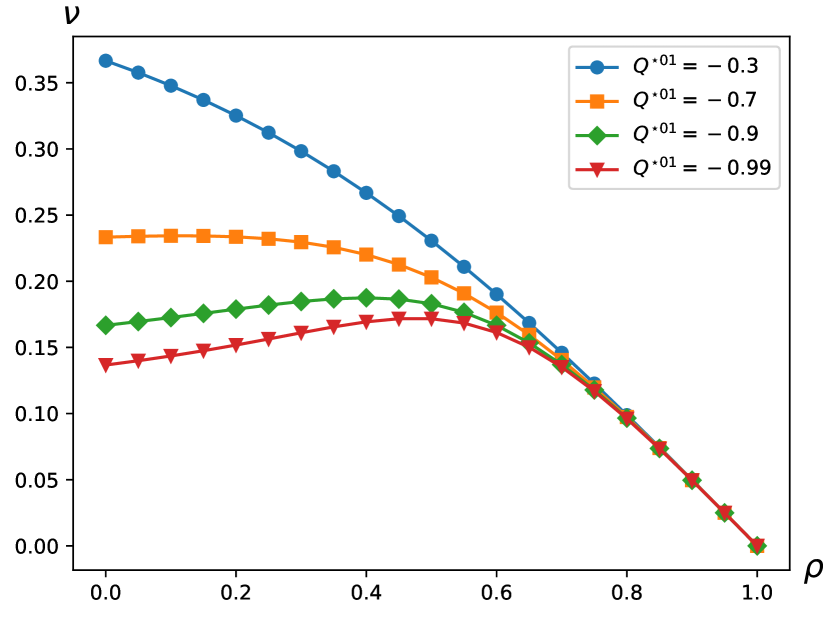
(b) Average velocity $\nu$

Figure 10: Average current $j$ and velocity $\nu$ as functions of ant density $\rho$. $Q^{\star}=1,q^{\star}=0.25,q^{\star 01}=-0.2,f^{\star}=0.5$ with different values of $Q^{\star 01}=-0.3;-0.7;-0.9;-0.99$.

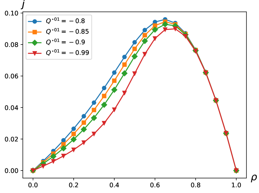
(a) Average current $j$

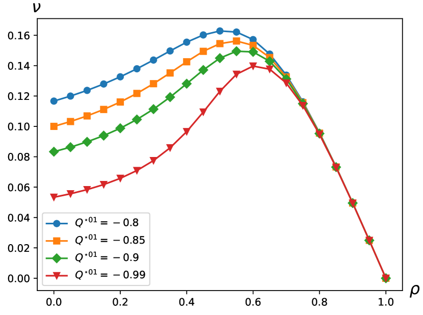
(b) Average velocity $\nu$

Figure 11: Average current $j$ and velocity $\nu$ as functions of ant density $\rho$. $Q^{\star}=1,q^{\star}=0.25,q^{\star 01}=-0.7,f^{\star}=0.5$ with different values of $Q^{\star 01}=-0.8;-0.85;-0.9;-0.99$.

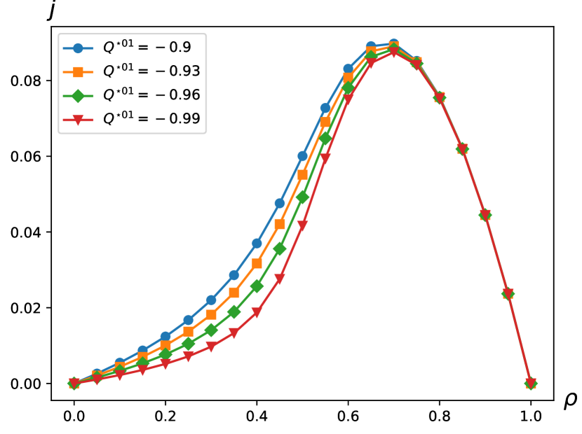
(a) Average current $j$

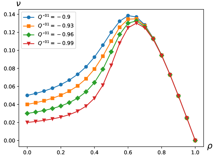
(b) Average velocity $\nu$

Figure 12: Average current $j$ and velocity $\nu$ as functions of ant density $\rho$. $Q^{\star}=1,q^{\star}=0.25,q^{\star 01}=-0.9,f^{\star}=0.5$ with different values of $Q^{\star 01}=-0.9;-0.93;-0.96;-0.99$.

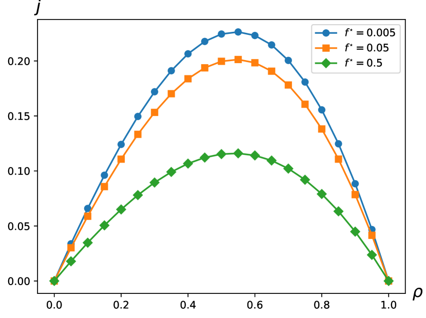
(a) Average current $j$

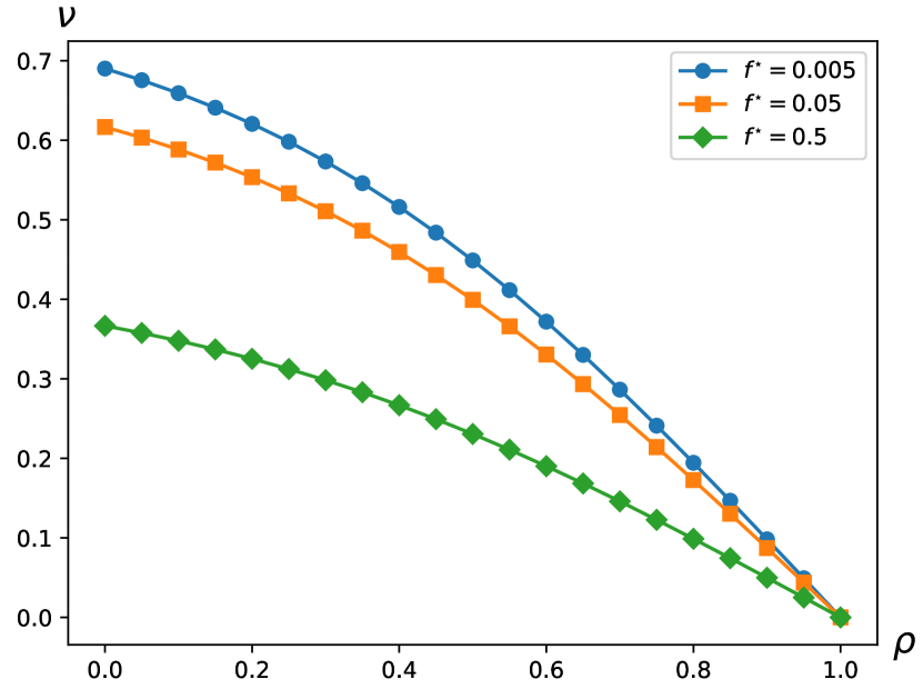
(b) Average velocity $\nu$

Figure 13: Average current $j$ and velocity $\nu$ as functions of ant density $\rho$. $Q^{\star}=1,q^{\star}=0.25,q^{\star 01}=-0.2,Q^{\star 01}=-0.3$ with different values of $f^{\star}=0.005;0.05;0.5$.

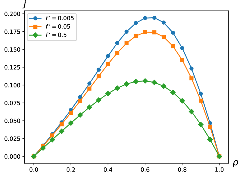
(a) Average current $j$

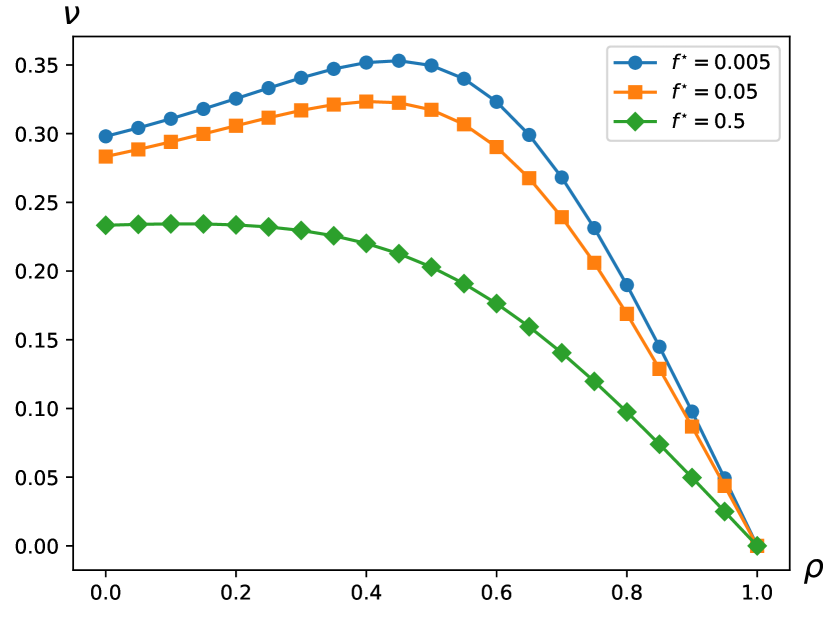
(b) Average velocity $\nu$

Figure 14: Average current $j$ and velocity $\nu$ as functions of ant density $\rho$. $Q^{\star}=1,q^{\star}=0.25,q^{\star 01}=-0.2,Q^{\star 01}=-0.7$ with different values of $f^{\star}=0.005;0.05;0.5$.

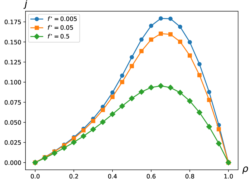
(a) Average current $j$

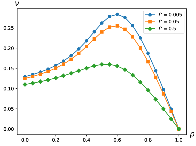
(b) Average velocity $\nu$

Figure 15: Average current $j$ and velocity $\nu$ as functions of ant density $\rho$. $Q^{\star}=1,q^{\star}=0.25,q^{\star 01}=-0.6,Q^{\star 01}=-0.87$ with different values of $f^{\star}=0.005;0.05;0.5$.

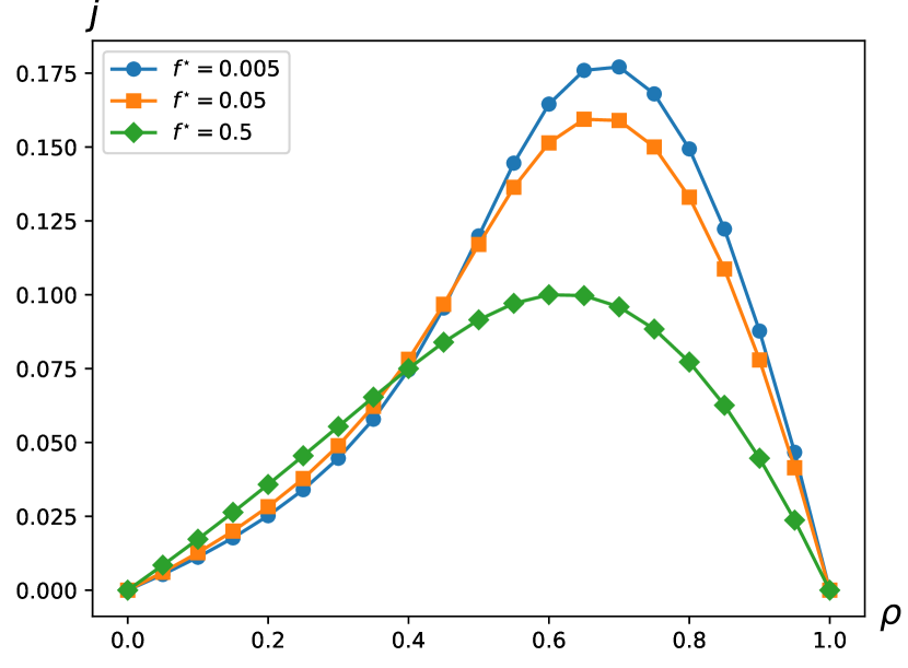
(a) Average current $j$

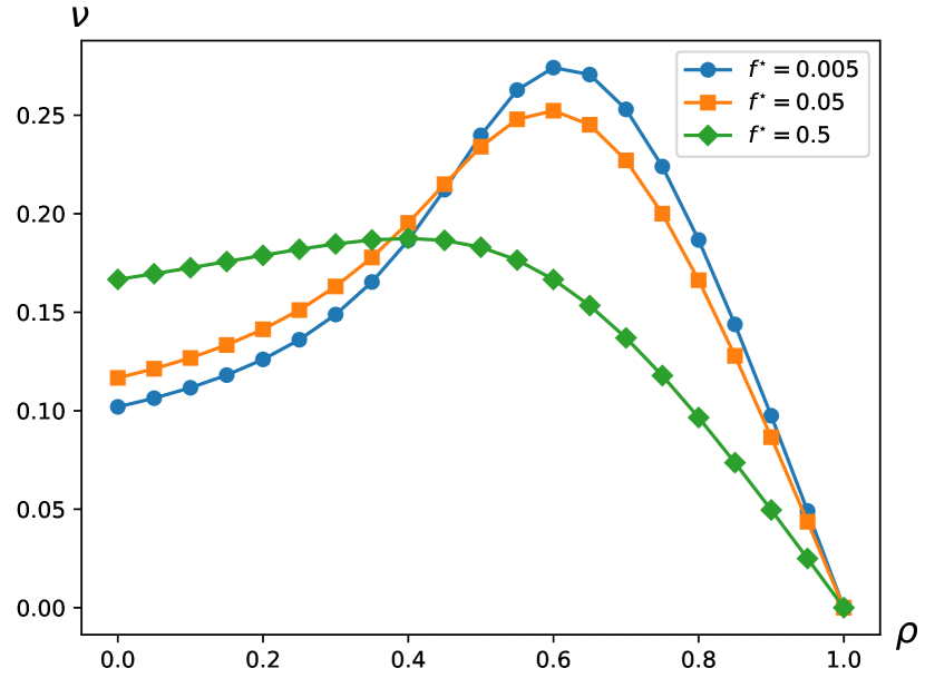
(b) Average velocity $\nu$

Figure 16: Average current $j$ and velocity $\nu$ as functions of ant density $\rho$. $Q^{\star}=1,q^{\star}=0.25,q^{\star 01}=-0.2,Q^{\star 01}=-0.9$ with different values of $f^{\star}=0.005;0.05;0.5$.

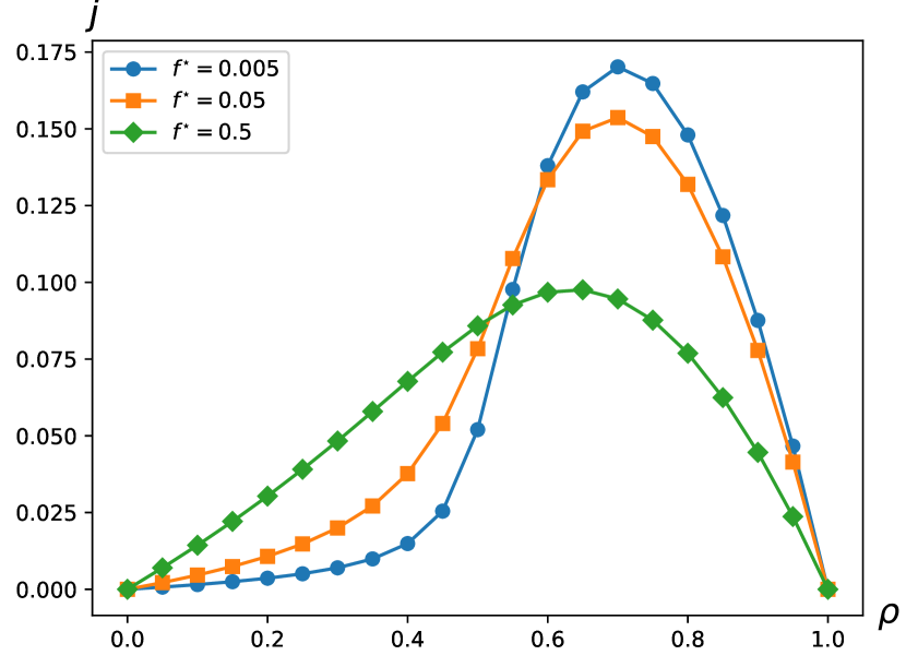
(a) Average current $j$

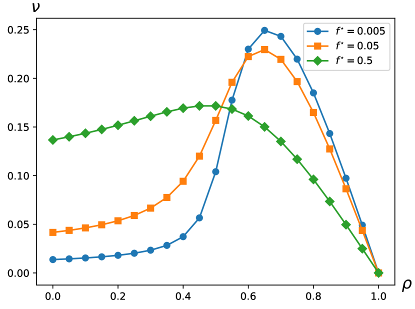
(b) Average velocity $\nu$

Figure 17: Average current $j$ and velocity $\nu$ as functions of ant density $\rho$. $Q^{\star}=1,q^{\star}=0.25,q^{\star 01}=-0.2,Q^{\star 01}=-0.99$ with different values of $f^{\star}=0.005;0.05;0.5$.

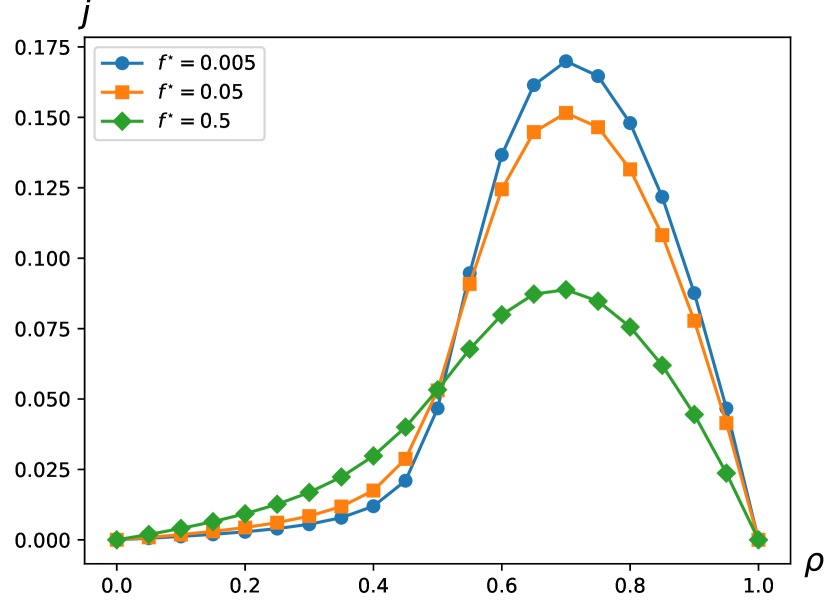
(a) Average current $j$

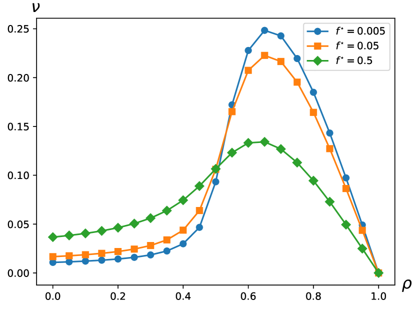
(b) Average velocity $\nu$

Figure 18: Average current $j$ and velocity $\nu$ as functions of ant density $\rho$. $Q^{\star}=1,q^{\star}=0.25,q^{\star 01}=-0.8,Q^{\star 01}=-0.99$ with different values of $f^{\star}=0.005;0.05;0.5$.

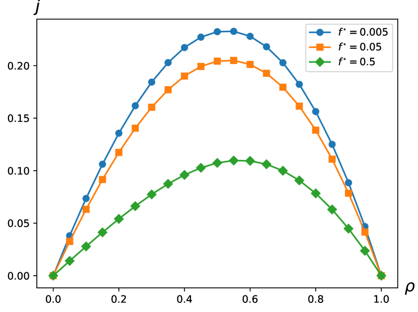
(a) Average current $j$

(b) Average velocity $\nu$

Figure 19: Average current $j$ and velocity $\nu$ as functions of ant density $\rho$. $Q^{\star}=1,q^{\star}=0.25,Q^{\star 01}=-0.2,q^{\star 01}=-0.9,$ with different values of $f^{\star}=0.005;0.05;0.5$.

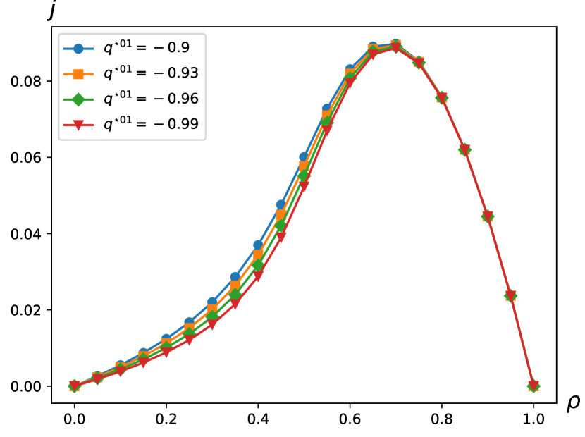
(a) Average current $j$

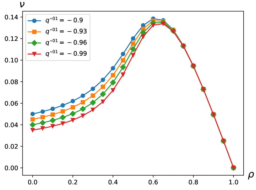
(b) Average velocity $\nu$

Figure 20: Average current $j$ and velocity $\nu$ as functions of ant density $\rho$. $Q^{\star}=1,q^{\star}=0.25,Q^{\star 01}=-0.9,f^{\star}=0.5$ with different values of $q^{\star 01}=-0.9;-0.93;-0.96$.

4 Discussion on average current and velocity

For convenience in the discussion below, it is important to note that the non-monotonic trend occurs when the average velocity reaches an intermediate maximum at a density $\rho_{m}$ within the range of $(0,1)$. As mentioned earlier, we examine how the neighboring-effect parameters $Q^{\star 01}$ and $q^{\star 01}$, along with the evaporating rate $f^{\star}$, influence the average current and velocity of ants in two scenarios: when $Q^{\star 01}\leq q^{\star 01}$ and when $Q^{\star 01}\geq q^{\star 01}$. Refer to Figs. 7 to 18 for the former case and Figs. 19 and 20 for the latter. Notice that in all figures in the previous section, the values of the neighboring-effect parameters $q^{\star 01}$ and $Q^{\star 01}$ are chosen as negative to indicate that pairs of ants locating neighboring sites enhance the rates. We will classify $Q^{\star 01}$ and $q^{\star 01}$ as either strong or weak depending on their proximity to $-1$ or $0$, respectively.

In the first scenario, we observe the impact of parameter $Q^{\star 01}$ across Figs. 7 to 12. At first glance, the average current and velocity decrease as $Q^{\star 01}$ decreases. This scenario explores two cases: one characterized by small values of $f^{\star}$ (close to 0), indicating a low probability of pheromone evaporation, as depicted in Figs. 7, 8, 9, and another characterized by large values of $f^{\star}$ (close to 1), indicating a high probability of pheromone evaporation, as shown in Figs. 10, 11, 12.

In the second case, when $q^{\star 01}$ is relatively weak, close to 0 (see Fig. 10), two scenarios emerge: one where $Q^{\star 01}$ is weak (close to 0) and another where it is strong (close to -1). When $Q^{\star 01}$ is not significantly strong, the model behaves similarly to TASEP, with the average velocity decreasing as density increases and the average current exhibiting symmetry. However, when $Q^{\star 01}$ is very strong, although a non-monotonic trend appears, it is not strongly evident. The trend becomes clearer when $q^{\star 01}$ is considerably strong (see Figs. 11 and 12).

In the first case of the first scenario, i.e., when $f^{\star}$ is small, a non-monotonic trend appears more evident compared to the second case. This non-monotonic trend emerges when $f^{\star}$ is small, as concluded in [8]. When both values of $q^{\star 01}$ and $Q^{\star 01}$ are weak, the model behaves also similarly to TASEP (symmetry of current and linear decrease of the velocity). Similarly to the second case, when both values are strong, the non-monotonic trend becomes clearer (see Figs. 8 and 9).

In the first scenario, we also examine the impact of parameter $f^{\star}$, as shown in Figs. 13, 14 and 15 for both $q^{\star 01}$ and $Q^{\star 01}$ being not so strong, and in Figs. 16, 17 and 18 when $Q^{\star 01}$ is very strong. In the former case, both current and velocity increase as $f^{\star}$ decreases. Additionally, when both $q^{\star 01}$ and $Q^{\star 01}$ are weak (Fig. 13), the average velocity decreases monotonically, similar to TASEP. When the value of $Q^{\star 01}$ is not as weak, as depicted in Figs. 14 and 15, the non-monotonic trend becomes clearer, especially with smaller $f^{\star}$. Interestingly, in the latter case (Figs. 16, 17 and 18), at low density, the current and velocity are greater when the value of $f^{\star}$ is larger. However, at high density, the current and velocity are smaller when the value of $f^{\star}$ is larger.

In the second scenario, where $Q^{\star 01}\geq q^{\star 01}$, we initially observe situations where $Q^{\star 01}$ is weak. In this case, it seems that the value of $q^{\star 01}$ has minimal impact on the average current and velocity. Consequently, we focus solely on the effect of the value $f^{\star}$ on these quantities, while keeping $Q^{\star 01}$ and $q^{\star 01}$ fixed, as depicted in Fig. 19. Here, the current and velocity behave similarly to those in TASEP even for $f^{\star}$ very small. The same holds true when $Q^{\star 01}$ is weak and $f^{\star}$ is close to 0, meaning that variations in $q^{\star 01}$ do not significantly alter the shapes of the current and velocity curves. However, when $Q^{\star 01}$ is strong, the influence of $q^{\star 01}$ on these quantities becomes slightly more apparent, as shown in Fig. 20. In this case, a non-monotonic trend also emerges.

5 Conclusion

We have presented an exactly solvable model for single-lane unidirectional ant traffic, drawing from the dynamics proposed by Chowdhury et al. However, our model utilizes random-sequential updates instead of the parallel updates used in the original model. Additionally, we introduced neighboring-effect parameters in our model, adjustable to better align with experimental data.

On the one hand, our results closely resemble those of Chowdhury et al. in explaining the non-monotonic trend of collective ant velocity. On the other hand, our model unveils an intriguing phenomenon absent in Chowdhury et al.’s work. Specifically, when the neighboring-effect parameters are strong, at low densities, the average current and velocity can exceed those at higher probabilities of evaporation. This behavior reverses at high densities, where smaller probabilities of evaporation yield greater average current and velocity.

Appendices

Appendix A Stationary conditions

We will outline a method for determining the conditions on the parameters present in the rates (7)–(9) to ensure that the process’s invariant measure aligns with the form described in (11), i.e., we will show how to obtain the constraints (15)–(20). To accomplish this, we will utilize the approach introduced in [4]. First, we will map the process onto a corresponding headway structure. Then, by using a discrete version of Noether’s theorem (39), we can rewrite the master equation of the process into a local divergence form when the system reaches equilibrium. From this point, one can determine the constraints.

A.1 Master equation

We represent the probability of the system being in configuration being in configuration $\boldsymbol{\eta}$ at time $t$ as $\mathbb{P}(\boldsymbol{\eta},t)$. The evolution of $\mathbb{P}(\boldsymbol{\eta},t)$ over time is governed by the master equation

$$\begin{split}\dfrac{d}{dt}\mathbb{P}(\boldsymbol{\eta},t)=\sum_{i=1}^{N}\bigg{(}q_{i}(\boldsymbol{\eta}_{1}^{i})\mathbb{P}(\boldsymbol{\eta}_{1}^{i},t)+Q_{i}(\boldsymbol{\eta}_{2}^{i})&\mathbb{P}(\boldsymbol{\eta}_{2}^{i},t)+f_{i}(\boldsymbol{\eta}_{3}^{i})\mathbb{P}(\boldsymbol{\eta}_{3}^{i},t)\\ &-(q_{i}(\boldsymbol{\eta})+Q_{i}(\boldsymbol{\eta})+f_{i}(\boldsymbol{\eta}))\mathbb{P}(\boldsymbol{\boldsymbol{\eta}},t)\bigg{)}.\end{split}$$ (33)

Here, $\boldsymbol{\eta}_{1}^{i}$ represents the configuration leading to $\boldsymbol{\eta}$ before the forward translocation of particle $i$ in state 1 (with $x_{i}^{1}=x_{i}-1$ and $s_{i}^{1}=3-s_{i}$), $\boldsymbol{\eta}_{2}^{i}$ signifies the configuration leading to $\boldsymbol{\boldsymbol{\eta}}$ before the forward translocation of particle $i$ in state 2 ($x_{i}^{2}=x_{i}-1$ and $s_{i}^{2}=s_{i}$), and $\boldsymbol{\eta}_{3}^{i}$ denotes the configuration $\boldsymbol{\eta}$ before the pheromone at site $x_{i}$ evaporates ($x_{i}^{3}=x_{i}$ and $s_{i}^{3}=3-s_{i}$).

At equilibrium, the master equation (33) does not depend on time, i.e., $\dfrac{d}{dt}\mathbb{\pi}(\boldsymbol{\eta},t)=0$. Thus,

$$\sum_{i=1}^{N}\big{(}q_{i}(\boldsymbol{\eta}_{1}^{i})\pi(\boldsymbol{\eta}_{1}^{i})+Q_{i}(\boldsymbol{\eta}_{2}^{i})\pi(\boldsymbol{\eta}_{2}^{i})+f_{i}(\boldsymbol{\eta}_{3}^{i})\pi(\boldsymbol{\eta}_{3}^{i})-(q_{i}(\boldsymbol{\eta})+Q_{i}(\boldsymbol{\eta})+f_{i}(\boldsymbol{\eta}))\pi(\boldsymbol{\boldsymbol{\eta}})\big{)}=0.$$ (34)

Dividing both sides of (34) by $\pi(\boldsymbol{\boldsymbol{\eta}})$, one obtains

$$\sum_{i=1}^{N}\big{(}q_{i}(\boldsymbol{\eta}_{1}^{i})\dfrac{\pi(\boldsymbol{\eta}_{1}^{i})}{\pi(\boldsymbol{\eta})}+Q_{i}(\boldsymbol{\eta}_{2}^{i})\dfrac{\pi(\boldsymbol{\eta}_{2}^{i})}{\pi(\boldsymbol{\eta})}+f_{i}(\boldsymbol{\eta}_{3}^{i})\dfrac{\pi(\boldsymbol{\eta}_{3}^{i})}{\pi(\boldsymbol{\eta})}-(q_{i}(\boldsymbol{\eta})+Q_{i}(\boldsymbol{\eta})+f_{i}(\boldsymbol{\eta}))\big{)}=0.$$ (35)

For convenience in writing, let us denote the following quantities

$$D_{i}(\boldsymbol{\eta)} =q_{i}(\boldsymbol{\eta}_{1}^{i})\dfrac{\pi(\boldsymbol{\eta}_{1}^{i})}{\pi(\boldsymbol{\eta})}-q_{i}(\boldsymbol{\eta}),$$ (36)

$$E_{i}(\boldsymbol{\eta)} =Q_{i}(\boldsymbol{\eta}_{2}^{i})\dfrac{\pi(\boldsymbol{\eta}_{2}^{i})}{\pi(\boldsymbol{\eta})}-Q_{i}(\boldsymbol{\eta}),$$ (37)

$$F_{i}(\boldsymbol{\eta}) =f_{i}(\boldsymbol{\eta}_{3}^{i})\dfrac{\pi(\boldsymbol{\eta}_{3}^{i})}{\pi(\boldsymbol{\eta})}-f_{i}(\boldsymbol{\eta}).$$ (38)

Because of the periodicity, the master equation $\eqref{mas_eq2}$ is satisfied if one has

$$D_{i}(\boldsymbol{\eta})+E_{i}(\boldsymbol{\eta})+F_{i}(\boldsymbol{\eta})=\Phi_{i}(\boldsymbol{\eta})-\Phi_{i+1}(\boldsymbol{\eta}).$$ (39)

This condition applies to all configurations of the system, characterized by a set of functions $\Phi_{i}(\boldsymbol{\eta})$ that adhere to the condition $\Phi_{N+1}(\boldsymbol{\eta)}=\Phi_{1}(\boldsymbol{\eta})$. One can consider the lattice divergence condition (39) as Noether’s theorem in discrete form. The specific forms of the functions $\Phi_{i}$ will be detailed in the subsequent subsection.

A.2 Mapping to the headway process

In addition to specifying a system’s configuration $\boldsymbol{\eta}=(\eta_{1},...,\eta_{L})$ by its position and state vectors $\textbf{x}=(x_{1},...,x_{N})$ and $\textbf{s}=(s_{1},...,s_{N})$ respectively, it can also be determined by the state vector along with the headway vector $\textbf{m}=(m_{1},...,m_{N})$. Here, $m_{i}$ represents the number of empty sites between the $i$-th and $(i+1)$-th particles, i.e., one has $m_{i}=x_{i+1}-(x_{i}+1)\mod L$.

To represent a headway of length $r$, instead of using $\delta_{m_{i},r}$, we adopt the concise notation $\theta_{i}^{r}$. Specifically, we define

$$\theta_{i}^{r}:=\delta_{m_{i},r}=\delta_{x_{i+1},x_{i}+1+r}.$$ (40)

Again, concerning the headway variable, the index $i$ is also considered modulo $N$, implying $\theta_{0}^{r}\equiv\theta_{N}^{r}$.

Because of steric hard-core repulsion, the $i$-th particle undergoes a forward translocation from $x_{i}$ to $x_{i}+1$, corresponding to the transition $(m_{i-1},m_{i})\to(m_{i-1}+1,m_{i}-1)$, whenever $m_{i}>0$. Expressed in the new stochastic variables $\boldsymbol{\zeta}=(\textbf{m},\textbf{s})$, where m represents the distance vector and s is the state vector, the invariant distribution (14) can be reformulated as

$$\tilde{\pi}(\boldsymbol{\zeta})=\dfrac{1}{\tilde{Z}}\prod_{i=1}^{N}x^{3/2-s_{i}}y^{-\theta_{i}^{0}},$$ (41)

where $\tilde{Z}$ is the partition function. Additionally, the transition rates (7)–(9) can be rewritten as

$$\tilde{q}_{i}(\boldsymbol{\zeta}) =q^{\star}\delta_{s_{i},1}(1+q^{\star 01}\theta_{i}^{1})(1-\theta_{i}^{0}),$$ (42)

$$\tilde{Q}_{i}(\boldsymbol{\zeta}) =Q^{\star}\delta_{s_{i},2}(1+Q^{\star 01}\theta_{i}^{1})(1-\theta_{i-1}^{0}),$$ (43)

$$\tilde{f}_{i}(\boldsymbol{\zeta}) =f^{\star}\delta_{s_{i},2}(1+f^{1\star}\theta_{i-1}^{0}+f^{\star 1}\theta_{i}^{0}+f^{10\star}\theta_{i-1}^{1}+f^{\star 01}\theta_{i}^{1}).$$ (44)

Given configuration $\boldsymbol{\zeta}$, let $\boldsymbol{\zeta}^{i,1}$ and $\boldsymbol{\zeta}^{i,2}$ represent configurations resulting from forward translocation when the state of particle $i$ is 1 and 2, respectively. Additionally, let $\boldsymbol{\zeta}^{i,3}$ denote the configuration leading to $\boldsymbol{\zeta}$ before pheromone evaporation at site $x_{i}$. Thus, configurations $\boldsymbol{\zeta}^{i,1}$, $\boldsymbol{\zeta}^{i,2}$, and $\boldsymbol{\zeta}^{i,3}$ are defined through the distance and state vectors by

$$m^{i,1}_{j}:=m_{j}+\delta_{j,i-1}-\delta_{j,i}\ \text{and }\ s^{i,1}_{j}:=s_{j}+(3-2s_{j})\delta_{j,i},$$ (45)

$$m^{i,2}_{j}:=m_{j}+\delta_{j,i-1}-\delta_{j,i}\ \text{and }\ s^{i,2}_{j}:=s_{j},$$ (46)

$$m_{j}^{i,3}:=m_{j}\ \text{and }\ s_{j}^{i,3}:=s_{j}+(3-2s_{j})\delta_{j,i}.$$ (47)

This yields the master equation for the headway process

$$\dfrac{d\mathbb{P}(\boldsymbol{\zeta},t)}{dt}=\sum_{i=1}^{N}H_{i}(\boldsymbol{\zeta},t)$$ (48)

with

$$\begin{split}H_{i}(\boldsymbol{\zeta},t)=&\ \ \tilde{q}_{i}(\boldsymbol{\zeta}^{i,1})\mathbb{P}(\boldsymbol{\zeta}^{i,1},t)-\tilde{q}_{i}(\boldsymbol{\zeta})\mathbb{P}(\boldsymbol{\zeta},t)+\tilde{Q}_{i}(\boldsymbol{\zeta}^{i,2})\mathbb{P}(\boldsymbol{\zeta}^{i,2},t)-\tilde{Q}_{i}(\boldsymbol{\zeta})\mathbb{P}(\boldsymbol{\zeta},t)\\ &+\tilde{f}_{i}(\boldsymbol{\zeta}^{i,3})\mathbb{P}(\boldsymbol{\zeta}^{i,3},t)-\tilde{f}_{i}(\boldsymbol{\zeta})\mathbb{P}(\boldsymbol{\zeta},t)\end{split}$$ (49)

where

$$\tilde{q}_{i}(\boldsymbol{\zeta}^{i,1}) =q^{\star}\delta_{s_{i},2}(1+d^{\star 01}\theta_{i}^{0})(1-\theta_{i-1}^{0}),$$ (50)

$$\tilde{Q}_{i}(\boldsymbol{\zeta}^{i,2}) =Q^{\star}\delta_{s_{i},2}(1+Q^{\star 01}\theta_{i}^{0})(1-\theta_{i-1}^{0}),$$ (51)

$$\tilde{f}_{i}(\boldsymbol{\zeta}^{i,3}) =f^{\star}\delta_{s_{i},1}(1+f^{1\star}\theta_{i-1}^{0}+f^{\star 1}\theta_{i}^{0}+f^{10\star}\theta_{i-1}^{1}+f^{\star 01}\theta_{i}^{1}).$$ (52)

Thus, at equilibrium, the master equation (48) yields

$$\begin{split}\sum_{i=1}^{N}\bigg{(}\tilde{q}_{i}(\boldsymbol{\zeta}^{i,1})\tilde{\pi}(\boldsymbol{\zeta}^{i,1})+\tilde{Q}_{i}(\boldsymbol{\zeta}^{i,2})\tilde{\pi}(\boldsymbol{\zeta}^{i,2})&+\tilde{f}_{i}(\boldsymbol{\zeta}^{i,3})\tilde{\pi}(\boldsymbol{\zeta}^{i,3})\\ &-\big{(}\tilde{q}_{i}(\boldsymbol{\zeta})+\tilde{Q}_{i}(\boldsymbol{\zeta})+\tilde{f}_{i}(\boldsymbol{\zeta})\big{)}\tilde{\pi}(\boldsymbol{\zeta})\bigg{)}=0.\end{split}$$ (53)

Before writing the local divergence condition for the headway process, which is equivalent to (39), we establish notation

$$\tilde{D}_{i}(\boldsymbol{\zeta}) =\tilde{q}_{i}(\boldsymbol{\zeta}^{i,1})\dfrac{\tilde{\pi}(\boldsymbol{\zeta}^{i,1})}{\tilde{\pi}(\boldsymbol{\zeta})}-\tilde{q}_{i}(\boldsymbol{\zeta}),$$ (54)

$$\tilde{E}_{i}(\boldsymbol{\zeta}) =\tilde{Q}_{i}(\boldsymbol{\zeta}^{i,2})\dfrac{\tilde{\pi}(\boldsymbol{\zeta}^{i,2})}{\tilde{\pi}(\boldsymbol{\zeta})}-\tilde{Q}_{i}(\boldsymbol{\zeta}),$$ (55)

$$\tilde{F}_{i}(\boldsymbol{\zeta}) =\tilde{f}_{i}(\boldsymbol{\zeta}^{i,3})\dfrac{\tilde{\pi}(\boldsymbol{\zeta}^{i,3})}{\tilde{\pi}(\boldsymbol{\zeta})}-\tilde{f}_{i}(\boldsymbol{\zeta}).$$ (56)

One has

$$\theta_{j}^{p}(\boldsymbol{\zeta}^{i,1})=\delta_{m_{j}+\delta_{j,i-1}-\delta_{j,i},p}=\theta_{j}^{p-\delta_{j,i-1}+\delta_{j,i}}(\boldsymbol{\zeta})\text{ and }\delta_{s_{i}^{i,1},\alpha}=\delta_{s_{i},3-\alpha},$$ (57)

$$\theta_{j}^{p}(\boldsymbol{\zeta}^{i,2})=\delta_{m_{j}+\delta_{j,i-1}-\delta_{j,i},p}=\theta_{j}^{p-\delta_{j,i-1}+\delta_{j,i}}(\boldsymbol{\zeta})\text{ and }\delta_{s_{i}^{i,2},\alpha}=\delta_{s_{i},\alpha},$$ (58)

$$\theta_{j}^{p}(\boldsymbol{\zeta}^{i,3})=\theta_{j}^{p}(\boldsymbol{\zeta})\text{ and }\delta_{s_{i}^{i,3},\alpha}=\delta_{s_{i},3-\alpha}.$$ (59)

Thus, one gets

$$\dfrac{\tilde{\pi}(\boldsymbol{\zeta}^{i,1})}{\tilde{\pi}(\boldsymbol{\zeta})} =x^{3-2s_{i}}y^{\theta_{i-1}^{0}-\theta_{i-1}^{1}+\theta_{i}^{0}},$$ (60)

$$\dfrac{\tilde{\pi}(\boldsymbol{\zeta}^{i,2})}{\tilde{\pi}(\boldsymbol{\zeta})} =y^{\theta_{i-1}^{0}-\theta_{i-1}^{1}+\theta_{i}^{0}},$$ (61)

$$\dfrac{\tilde{\pi}(\boldsymbol{\zeta}^{i,3})}{\tilde{\pi}(\boldsymbol{\zeta})} =x^{3-2s_{i}}.$$ (62)

Similarly to (39), the master equation $\eqref{mas_eq4}$ is satisfied if one requires

$$\tilde{D}_{i}+\tilde{E}_{i}+\tilde{F}_{i}=\tilde{\Phi}_{i-1}-\tilde{\Phi}_{i},$$ (63)

where $\tilde{\Phi}_{i}$ is of the form $\tilde{\Phi}_{i}=(a+b\theta_{i}^{0}+c\theta_{i}^{1})(\delta_{s_{i},1}+\delta_{s_{i},2})=a+b\theta_{i}^{0}+c\theta_{i}^{1}$. Note that $\tilde{\Phi}_{i}$ must conform to this form, as $\tilde{D}_{i}$, $\tilde{E}_{i}$, and $\tilde{F}_{i}$ are contingent upon the state of particle $i$ and variables $\theta_{i-1}^{0}$, $\theta_{i-1}^{1}$, $\theta_{i}^{0}$, $\theta_{i}^{1}$, all of which belong to the set $\{0,1\}$. By examining all possible cases of (63), one can initially obtain

$$b =\dfrac{-q^{\star}(1+q^{1\star})-xQ^{\star}(1+Q^{1\star})}{1+x},$$ (64)

$$c =\dfrac{q^{\star}q^{\star 01}+xQ^{\star}Q^{\star 01}}{1+x},$$ (65)

and then one gets the stationary conditions (15)–(20). However, we shall give a clearer proof of the above claim in the next subsection after knowing the results.

A.3 Proof of Theorem 2.1

To prove Theorem 2.1, it suffices to demonstrate that (63) holds for all configurations. Note that (63) depends on distance variables $\theta_{i-1}^{0},\theta_{i-1}^{1},\theta_{i}^{0},\theta_{i}^{1}$, or equivalently, on $m_{i-1}$ and $m_{i}$. Let us consider the various cases of $m_{i-1}$ and $m_{i}$ as follows:

• If $m_{i-1}$ and $m_{i}$ are both greater than 1, one has $\tilde{D}_{i}=x^{-1}q^{\star}\delta_{s_{i},2}-q^{\star}\delta_{s_{i},1},\tilde{E}_{i}=0,\tilde{F}_{i}=xf^{\star}\delta_{s_{i},1}-f^{\star}\delta_{s_{i},2}$. Note that in this case, the right-hand side of (63) is 0. If the state of the particle is 1, meaning $s_{i}=1$, then $\tilde{D}_{i}+\tilde{E}_{i}+\tilde{F}_{i}=-q^{\star}+xf^{\star}$ which is equal to 0 due to (15). Similarly, for $s_{i}=2$, $\tilde{D}_{i}+\tilde{E}_{i}+\tilde{F}_{i}=x^{-1}q^{\star}-f^{\star}$, also equaling to 0 due to (15). Thus, (63) holds in this case.

• If $m_{i-1}>1,m_{i}=1$, one has $\tilde{D}_{i}=x^{-1}q^{\star}\delta_{s_{i},2}-q^{\star}\delta_{s_{i},1}(1+q^{\star 01})$, $\tilde{E}_{i}=Q^{\star}\delta_{s_{i},2}-Q^{\star}\delta_{s_{i},2}(1+Q^{\star 01})$, $\tilde{F}_{i}=(x\delta_{s_{i},1}-\delta_{s_{i},2})f^{\star}(1+f^{\star 01})$. In this case, the right-hand side of (63) is $-c$. If $s_{i}=1$, then $\tilde{D}_{i}+\tilde{E}_{i}+\tilde{F}_{i}=-q^{\star}(1+q^{\star 01})+xf^{\star}(1+f^{\star 01})$. It can be verified from (15) and (20) that $\tilde{D}_{i}+\tilde{E}_{i}+\tilde{F}_{i}=-c$, where $c$ is defined in (65). Thus, (63) holds for this case. Similarly, for $s_{i}=2$, (63) holds as well.

• For the remaining cases ($m_{i-1}>1,m_{i}=0$; $m_{i-1}=1,m_{i}>1$; $m_{i-1}=0,m_{i}>1$; $m_{i-1}=1,m_{i}=1$; $m_{i-1}=1,m_{i}=0$; $m_{i-1}=0,m_{i}=1$; $m_{i-1}=0,m_{i}=0$), similar reasoning demonstrates that (63) holds.

Thus, the proof is complete.

Appendix B Partition function and headway distribution

Just like in previous studies [4, 5], instead using measure (14), we adopt the grand-canonical ensemble for ease of analysis, as defined by

$$\tilde{\pi}(\zeta)=\dfrac{1}{Z_{gc}}\prod_{i=1}^{N}x^{-3/2+s_{i}}y^{-\theta_{i}^{0}}z^{m_{i}},$$ (66)

where $Z_{gc}=(Z_{1}Z_{2})^{N}$ with

$$Z_{1}=\dfrac{1+(y-1)z}{1-z},\ \ Z_{2}=x^{1/2}+x^{-1/2}.$$ (67)

Here, the fugacity $z$ serves as a fugacity through which the particle density can be determined.

As one can observe, the partition function $Z_{gc}$ has a fixed form. Consequently, it is necessary to demonstrate the well-defined nature of the measure (66). To achieve this, it is crucial to establish the equivalence between the two measures (41) and (66), wherein a value of $z$ corresponding to a given particle density $\rho_{p}$ can always be found, ensuring that the probability of a configuration under both measures is identical. It is worth noting that this task was previously addressed in [4, 5], given the similarity between the grand-canonical ensemble form (66) and the one presented in the aforementioned papers. However, for the benefit of our readers, we rewrite the proof here. On the one hand, one can compute the mean headway using the grand-ensemble (66). Namely, one has

$$\langle m_{i}\rangle=\dfrac{1}{N}z\dfrac{d}{dz}\ln Z_{gc}=\dfrac{yz}{(1-z)(1+(y-1)z)}.$$ (68)

Here, $\langle\cdot\rangle$ indicates taking the expectation with respect to the distribution (66). On the other hand, the mean headway can be computed as $\langle m_{i}\rangle=\dfrac{1}{\rho_{p}}-1$, representing the average number of empty sites on the lattice per particle. Here, $\rho_{p}$ is the particle density. Thus, the value of $z$ can be determined by solving the following equation

$$(y-1)z^{2}+z\big{(}\dfrac{y\rho_{p}}{1-\rho_{p}}-y+2\big{)}-1=0.$$ (69)

Note that the quadratic equation above yields two solutions for $z$. However, the chosen value of $z$ must ensure that $Z_{gc}$ remains finite. This condition implies that $0\leq z<1$. Considering that $0<\rho_{p}\leq 1$, the value of $z$ can be selected as

$$z(\rho_{p},y)=1-\dfrac{1-\sqrt{1-4\rho_{p}(1-\rho_{p})(1-y^{-1})}}{2(1-\rho_{p})(1-y^{-1})}.$$ (70)

This selection guarantees the condition $0\leq z<1$.

When working with the grand-canonical ensemble (66) concerning the headway process, deriving the probability distribution for the gap between two particles is easily achieved, defined as

$$P_{h}(r)=\tilde{\pi}_{gc}(m_{i}=r).$$ (71)

Alternatively, we can express $P_{h}(r)$ as $\langle\theta_{i}^{r}\rangle_{gc}$, where the random variables $\theta_{i}^{r}$ are defined in equation (40). Therefore, the headway distribution can be expressed as

$$P_{h}(r)=\begin{cases}\dfrac{1-z}{1+(y-1)z}\ \ \text{ for }r=0,\\ yP_{h}(0)z^{r}\ \ \text{ for }r\geq 1.\end{cases}$$ (72)

References

References

- [1] C. Anderson and F.L.W Ratnieks,Task partitioning in insect societies: novel situations. The American Naturalist, 154(5):521–535, November 1999.
- [2] C. Anderson and F.L.W. Ratnieks,Task Partitioning in Insect Societies. I. Effect of Colony Size on Queueing Delay and Colony Ergonomic Efficiency. Insectes Sociaux, 47(2):198–199, May 2000.
- [3] C. Anderson and D.W. McShea,Individual versus social complexity, with particular reference to ant colonies. Biological Reviews, 76(2):211–237, May 2001.
- [4] V. Belitsky and G.M. Schütz, RNA Polymerase interactions and elongation rate. Journal of Theoretical Biology, 462:370–380, February 2019.
- [5] V. Belitsky and G.M. Schütz, Stationary RNA Polymerase fluctuations during transcription elongation. Physical Review E, 99(1), January 2019.
- [6] E. Bonabeau, M. Dorigo, and G. Theraulaz, Inspiration for optimization from social insect behaviour. Nature, 406(6791):39–42, July 2000.
- [7] T. Chou, K. Mallick, and R.K.P. Zia, Non-equilibrium statistical mechanics: from a paradigmatic model to biological transport. Reports on Progress in Physics, 74(11):116601, October 2011.
- [8] D. Chowdhury, V. Guttal, K. Nishinari, and A. Schadschneider, A cellular-automata model of flow in ant trails: non-monotonic variation of speed with density. Journal of Physics A: Mathematical and General, 35(41):L573–L577, October 2002.
- [9] I.D. Couzin, N.R. Franks, Self-organized lane formation and optimized traffic flow in army ants. Proceedings of the Royal Society of London. Series B: Biological Sciences, 270(1511):139–146, January 2003.
- [10] M. Dorigo, G. Di Caro, and L.M. Gambardella., Ant Algorithms for Discrete Optimization. Artificial Life , 5(2):137–172, April 1999.
- [11] M. Dorigo, E. Bonabeau, and G. Theraulaz., Swarm Intelligence: From Natural to Artificial Intelligence. Oxford University Press, 1999.
- [12] V. Epshtein, E. Nudler, Cooperation between RNA Polymerase molecules in transcription elongation. Science, 300(5620):801–805, May 2003.
- [13] V. Epshtein, Transcription through the roadblocks: the role of RNA Polymerase cooperation. The EMBO Journal, 22(18):4719–4727, September 2003.
- [14] M.R. Evans, T. Hanney, Nonequilibrium statistical mechanics of the zero-range process and related models. Journal of Physics A: Mathematical and General, 38(19):R195–R240, April 2005.
- [15] S. Gokce, O. Kayacan, A cellular automata model for ant trails. Pramana, 80(5):909–915, April 2013.
- [16] A. John, A. Schadschneider, D. Chowdhury, and K. Nishinari, Characteristics of ant-inspired traffic flow: Applying the social insect metaphor to traffic models. Swarm Intelligence, 2(1):25–41, March 2008.
- [17] A. John, A. Schadschneider, D. Chowdhury, and K. Nishinari, Trafficlike Collective Movement of Ants on Trails: Absence of a Jammed Phase. Physical Review Letters, 102(10), March 2009.
- [18] K. Johnson, L.F. Rossi, A mathematical and experimental study of ant foraging trail dynamics. Journal of Theoretical Biology, 241(2):360–369, July 2006.
- [19] S. Katz, J.L. Lebowitz, and H. Spohn, Nonequilibrium steady states of stochastic lattice gas models of fast ionic conductors. Journal of Statistical Physics, 34(3–4):497–537, February 1984.
- [20] M.J.B. Krieger, J.B. Billeter, and L. Keller, Ant-like task allocation and recruitment in cooperative robots. Nature, 406(6799):992–995, August 2000.
- [21] A. Kunwar, A. John, K. Nishinari, A. Schadschneider, and D. Chowdhury, Collective Traffic-like Movement of Ants on a Trail: Dynamical Phases and Phase Transitions. Journal of the Physical Society of Japan, 73(11):2979–2985, November 2004.
- [22] T.M. Liggett, Interacting Particle Systems. Springer Berlin Heidelberg, 2005.
- [23] C.T. MacDonald, J.H. Gibbs, and A.C. Pipkin, Kinetics of biopolymerization on nucleic acid templates. Biopolymers, 6(1):1–25, January 1968.
- [24] C.T. MacDonald and J.H. Gibbs, Concerning the kinetics of polypeptide synthesis on polyribosomes. Biopolymers, 7(5):707–725, May 1969.
- [25] K. Nishinari, D. Chowdhury, and A. Schadschneider, Cluster formation and anomalous fundamental diagram in an ant-trail model. Physical Review E, 67(3), March 2003.
- [26] N.P.N. Ngoc, H.A. Thi, General criterion applicable to exclusion processes with an Ising-like invariant measure. Chinese Journal of Physics, 88:618–631, April 2024.
- [27] F.L.W. Ratnieks and C. Anderson, Task partitioning in insect societies. Insectes Sociaux, 46(2):95–108, May 1999.
- [28] F.L.W. Ratnieks and C. Anderson, Task Partitioning in Insect Societies. II. Use of Queueing Delay Information in Recruitment. The American Naturalist, 154(5):536–548, November 1999.
- [29] A. Schadschneider, D. Chowdhury, and K. Nishinari, Stochastic transport in complex systems: from molecules to vehicles. Elsevier, Amsterdam, 2011.
- [30] G.M. Schütz, Exactly Solvable Models for Many-Body Systems Far from Equilibrium. Elsevier, page 1–251, 2001.
- [31] G.M. Schütz, Fluctuations in Stochastic Interacting Particle Systems. Springer International Publishing, page 67–134, 2019.
- [32] F. Spitzer, Interaction of Markov processes. Advances in Mathematics, 5(2):246–290, October 1970.