Abstract

We study the generalization capability of nearly-interpolating linear regressors: $\bm{\beta}$’s whose training error $\tau$ is positive but small, i.e., below the noise floor. Under a random matrix theoretic assumption on the data distribution and an eigendecay assumption on the data covariance matrix $\bm{\Sigma}$, we demonstrate that any near-interpolator exhibits rapid norm growth: for $\tau$ fixed, $\bm{\beta}$ has squared $\ell_{2}$-norm $\mathbb{E}[\|{\bm{\beta}}\|_{2}^{2}]=\Omega(n^{\alpha})$ where $n$ is the number of samples and $\alpha>1$ is the exponent of the eigendecay, i.e., $\lambda_{i}(\bm{\Sigma})\sim i^{-\alpha}$. This implies that existing data-independent norm-based bounds are necessarily loose. On the other hand, in the same regime we precisely characterize the asymptotic trade-off between interpolation and generalization. Our characterization reveals that larger norm scaling exponents $\alpha$ correspond to worse trade-offs between interpolation and generalization. We verify empirically that a similar phenomenon holds for nearly-interpolating shallow neural networks.

1 INTRODUCTION

Regularization (Nakkiran et al.,, 2020) and early stopping (Ji et al.,, 2021) are techniques to mitigate the effect of harmful overfitting by training models to nearly, rather than perfectly, interpolate the training data. A key question is: how do near-interpolators generalize?

A long line of work has investigated this question for perfect-interpolators. Zhang et al., (2017) noted the surprising phenomon that, even with noise, perfect-interpolators do not necessarily overfit catastrophically, and can still generalize to some extent. The phenomenon is later formalized as “benign overfitting” and proven to hold in linear regresion in Bartlett et al., (2020). Mallinar et al., (2022) introduced the more nuanced notion of tempered overfitting which is closer to the empirical observation in Zhang et al., (2017) that the test error of perfect-interpolators do degrade somewhat. Koehler et al., (2021) establish a setting under which benign overfitting can be explained by uniform bounds. However, to the best of our knowledge, no work have studied generalization of near-interpolating linear regression .

Our results. Under random matrix-theoretic and power-law spectra assumptions, we prove that nearly-interpolating ridge regressors have norms that grows rapidly (Theorem 1.6), implying that existing (non-asymptotic) generalization bounds are loose (Section 4.2). Moreover, we derive the exact formula relating the large-sample limit training and the testing error (Theorem 1.5), using the eigenlearning framework of Simon et al., (2023). Finally, we show that our theoretical results on near-interpolating ridge regressors are relevant empirically and can give insight into the behavior of early-stopped near-interpolating shallow neural networks.

Implications. Our result on the norm growth implies that existing data-independent bounds and possible extension are necessarily loose. See Section 4.2. Thus, in order to explain the learning capability of near-interpolators, there is a need to develop data-dependent generalization bounds.

On the other hand, our result allows the analysis of the trade-off between nearness of interpolation and generalization. Our result reveals delicate interplay between the overparametrization ratio and the power-law spectra exponent. In particular, for larger power-law spectra exponent implies larger asymptotic excess test error ratio of $5\%$- over $50\%$-noise floor interpolation, for instance. Put more simply, the harmfulness of overfitting depends on the data distribution. Moreover, this effect is stronger at high level of overparametrization (large $p/n$). (See Figure 2 and Figure 1-left panel.) Experimentally, this effect appears in shallow neural networks as well (Figure 4).

1.1 Related works

Near interpolation. Learning algorithms that (nearly) interpolate the training data, such as deep neural networks, have been surprisingly effective in practice despite conventional statistical wisdom suggesting otherwise (Zhang et al.,, 2021). Many practices in modern machine learning e.g., early stopped neural network and high-dimensional ridge regression, result in near- rather than perfect-interpolators (Ji et al.,, 2021; Kuzborskij and Szepesvári,, 2022). In terms of theory work, Ghosh and Belkin, (2022) provides a lower bounds on the test error for near-interpolators.

Power law spectra. Empirically, power law spectra arise in neural tangent kernels computed from practical networks for common datasets, e.g., MNIST (Velikanov and Yarotsky,, 2021) On the theory side, the power law spectra assumption has been used previously to analyze benign (Bartlett et al.,, 2020, Theorem 2) and tempered overfitting phenomena (Mallinar et al.,, 2022, Theorem 3.1).

Looseness of existing generalization bounds. Our work is motivated by the empirical evidence found by Wei et al., (2022) suggests that norms of kernel ridge regressors grow rapidly potentially beyond the purview of norm-based bound. We confirm that bounds similar to ones in Koehler et al., (2021, Corollary 1) grow to infinity. Even more refined bounds such as Koehler et al., (2021, Theorem 1) grow as $n$ goes to infinity. Therefore, our work suggests that explaining the generalization capability of near-interpolators will require new tools.

1.2 Notations

Throughout this work, we assume the setting of high-dimensional linear regression as described below. Let $n$ denote the number of samples and $p$ denote the feature dimension. Consider the setting where $n,p\to\infty$ at the same time. The sample-to-feature ratio is denoted $\gamma:=n/p\in\mathbb{R}_{>0}$ and the asymptotic sample-to-feature ratio is denoted $\gamma_{\ast}:=\lim_{n\to\infty}\gamma\in\mathbb{R}_{\geq 0}$. Here, $n$ is the fundamental parameter which $p$ depends on implicitly.

Let $X\in\mathbb{R}^{p}$ and $Y\in\mathbb{R}$ denote a random vector (resp. variable), referred to as the sample (resp. label). Suppose that $\bm{\beta}^{\star}\in\mathbb{R}^{p}$ is such that $Y=\varepsilon+X^{\top}\bm{\beta}^{\star}$ where $\varepsilon\in\mathbb{R}$ is a random variable denoting independent, zero mean noise, i.e., $\mathbb{E}[\varepsilon]=0$ and $\varepsilon\perp X$. Here $\perp$ denotes independence between random variables. The noise variance is denoted $\sigma^{2}:=\mathbb{E}[\varepsilon^{2}]$.

The training data is denoted $\{(x_{i},y_{i})\}_{i=1}^{n}$ where $x_{i}\in\mathbb{R}^{p}$ and $\varepsilon_{i}\in\mathbb{R}$ are i.i.d realizations of $X$ and of the noise, and $y_{i}=\varepsilon_{i}+x_{i}^{\top}\bm{\beta}^{\star}$. Let $\mathbf{X}=[x_{1},\dots,x_{n}]\in\mathbb{R}^{p\times n}$ be the data matrix obtained by horizontally stacking the $x_{i}$’s, and let $\mathbf{y}=(y_{1},\dots,y_{n})^{\top}\in\mathbb{R}^{n}$ be the (column vector) by concatenating the $y_{i}$’s. Likewise, define $\bm{\varepsilon}=(\varepsilon_{1},\dots,\varepsilon_{n})^{\top}\in\mathbb{R}^{n}$. For a positive integer $p$, let $\mathbf{I}_{p}$ denote the $p\times p$ identity matrix. Let $\bm{\beta}\in\mathbb{R}^{p}$ be arbitrary. The empirical training mean squared error (MSE) of $\bm{\beta}$ is denoted

$$\mathcal{E}_{\mathtt{train}}^{n}(\bm{\beta})=\frac{1}{n}\|\mathbf{X}^{\top}\bm{\beta}-\mathbf{y}\|_{2}^{2}.$$

Likewise, the expected test error of $\bm{\beta}$ is denoted

$$\mathcal{E}_{\mathtt{test}}^{n}(\bm{\beta})=\mathbb{E}[\|X^{\top}\bm{\beta}-Y\|_{2}^{2}].$$

Let $\hat{\bm{\Sigma}}:=n^{-1}\mathbf{X}\mathbf{X}^{\top}$ denote the sample covariance matrix and $\check{\mathbf{G}}:=n^{-1}\mathbf{X}^{\top}\mathbf{X}$ the (scaled) gram matrix. Let $\bm{\Sigma}:=\mathbb{E}[\hat{\bm{\Sigma}}]$ denote the population covariance.

We note that all quantities defined on the training data implicitly depend on $n$. When the dependencies need to be made explicit, we shall write $\bm{\beta}^{\star}_{n}$, $\hat{\bm{\Sigma}}_{n}$ and so on.

1.3 Our contributions

Recall the minimum norm near-interpolator:

Definition 1.1.

Let $\tau\in(0,\sigma^{2})$. The minimum norm $\tau$-near-interpolator is defined as

$$\underline{\smash{\bm{\beta}}}_{\tau}:=\mathrm{argmin}_{\bm{\beta}\in\mathbb{R}^{p}}\|\bm{\beta}\|_{2}^{2}\,\,s.t.\,\,\tfrac{1}{n}\|\mathbf{X}^{\top}\bm{\beta}-\mathbf{y}\|_{2}^{2}\leq\tau.$$ (1)

A $\tau$-near-interpolator (not necessarily of the minimum norm) is any $\bm{\beta}\in\mathbb{R}^{p}$ satisfying the inequality in (1).

In the overparameterized ($p>n$) regime, near-interpolators can often be realized by ridge regression:

Definition 1.2.

Let $\varrho>0$. The ridge regressor with regularizer $\varrho$ is defined as

$$\hat{\bm{\beta}}_{\varrho}:=\mathrm{argmin}_{\bm{\beta}\in\mathbb{R}^{p}}\tfrac{1}{n}\|\mathbf{X}^{\top}\bm{\beta}-\mathbf{y}\|_{2}^{2}+\varrho\|\bm{\beta}\|_{2}^{2}.$$ (2)

Main problems: For any $\tau\in(0,\sigma^{2})$, 1. find a sequence of regularizers $\{\varrho_{n}\}_{n}$ so that

$$\mathcal{E}_{\mathtt{train}}^{\ast}:=\lim_{n\to\infty}\mathbb{E}[\mathcal{E}_{\mathtt{train}}^{n}(\hat{\bm{\beta}}_{\varrho_{n}})]=\tau$$ (3)

where the expectation is over all sources of randomness and 2. compute the associated asymptotic test error:

$$\mathcal{E}_{\mathtt{test}}^{\ast}:=\lim_{n\to\infty}\mathcal{E}_{\mathtt{test}}^{n}(\hat{\bm{\beta}}_{\varrho_{n}}).$$ (4)

Definition 1.3.

Let $\tau\in(0,\sigma^{2})$ be arbitrary and $\{\varrho_{n}\}_{n}$ be any sequence of regularizers. If Equation 3 holds, then we say the sequence of regressors $\{\hat{\bm{\beta}}_{\varrho_{n}}\}_{n}$ is an asymptotic $\tau$-near interpolator with asymptotic test error given by Equation 4.

Assumption 1.4 (Power-law spectra).

Suppose there exists $\alpha>1$ such that the population data covariance matrix $\bm{\Sigma}=\mathrm{diag}(\lambda_{1},\cdots,\lambda_{p})$ where $\lambda_{i}=i^{-\alpha}$.

There are many examples of random matrix ensembles exhibiting power-law spectra in a broader sense than that of Assumption 1.4. For instance, see (Arous and Guionnet,, 2008; Mahoney and Martin,, 2019; Wang et al.,, 2024). For simplicity, we do not pursue a general setting and will consider the setting of Assumption 1.4.

The asymptotic test error of an asymptotic $\tau$-near interpolator can be calculated as follows. Let $F={}_{2}F_{1}$ denote the Gaussian Hypergeometric function (Dutka,, 1984, Eqn. (27)).

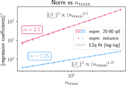
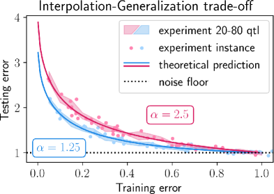
Figure 1: Left: Synthetic experiments validating the norm lower bound of norms of $0.2$-near-interpolators given by Proposition 1.7. The squared norms are fitted by least squares (in log-log space) to estimate the norm-growth exponent $\alpha$ using only data points. See Section 5 for additional experiment details. Right: Trade-off between the testing and training errors from Theorem 1.5. The solid curves are the parametrized curves whose $(x,y)$-coordinates are $(\mathcal{E}_{\mathtt{train}}^{\ast},\mathcal{E}_{\mathtt{test}}^{\ast})$ and parametrized by $k$ (which is in 1-to-1 correspondence with $r$ see Theorem 1.5). The scatter points, subsampled for visualization, denote ridge regression run results on the HDA model (Example 2.8). The colored ribbons denote the 20-80 quantiles for the scatter points. The horizontal dotted line denotes the noise $\sigma^{2}$ which is set to $1$ without the loss of generality.

Theorem 1.5 (Exact trade-off formula).

Let $\tau\in(0,\sigma^{2})$ be arbitrary. Suppose that $\sup_{n=1,2\dots}\|\bm{\beta}^{\star}\|_{2}<+\infty$, Assumption 1.4 holds, and $X=\bm{\Sigma}^{1/2}Z$ where $Z\sim\mathcal{N}(0,\mathbf{I}_{p})$. There exists unique number $k\in\mathbb{R}_{>0}$ such that that the following hold. Define the regularizer-factor

$$r:=1-\gamma_{\ast}^{-1}F(1,\tfrac{1}{\alpha};1+\tfrac{1}{\alpha};-k\gamma_{\ast}^{-\alpha})$$

and let $\varrho_{n}:=rn^{-\alpha}$. Then $\{\hat{\bm{\beta}}_{\varrho_{n}}\}_{n}$ is an asymptotic $\tau$-near interpolator whose asymptotic test error is

$$\mathcal{E}_{\mathtt{test}}^{\ast}=\sigma^{2}\frac{1}{1-\gamma_{\ast}^{-1}F(2,\tfrac{1}{\alpha};1+\tfrac{1}{\alpha};-k\gamma_{\ast}^{-\alpha})}.$$ (5)

Moreover, $\mathcal{E}^{\ast}_{\mathtt{test}}$ is a decreasing function w.r.t $\alpha$, fixing all other quantities.

The reason we call Theorem 1.5 an “exact trade-off formula” is that Equation 5 allows the calculate of the trade-off curve between train and test error (Figure 1-right). The fundamental parameter is $k$. The asymptotic testing error and training error, i.e., $\tau$, all depend on $k$ via monotonic 1-1 correspondences on the domain $k\in(k_{\mathtt{crit}},\infty)$. See Figure 3 below. Thus, the asymptotic testing error depends on the training error implicitly through $k$.

Figure 1-right panel demonstrates that, empirically, training and test MSEs concentrate closely around Equation 5. We further discuss in detail the implications of Theorem 1.5 after stating Proposition 3.2.

Figure 1-right shows that for near-interpolators, the test error does not degrade much when training below the noise floor. A natural question is if this can be explained by data-independent norm-based generalization bound such as the one found in Koehler et al., (2021). Our next result shows that the growth rate of an asymptotic $\tau$-near interpolator is superlinear:

Theorem 1.6 (Rapid norm growth).

In the situation of Theorem 1.5, for any $\tau\in(0,\sigma^{2})$, suppose $\varrho_{n}>0$ is a sequence of regularizers such that $\{\hat{\bm{\beta}}_{\varrho_{n}}\}_{n}$ is an asymptotic $\tau$-near interpolator. Then $\mathbb{E}[\|\hat{\bm{\beta}}_{\varrho_{n}}\|_{2}^{2}]=\Omega(n^{\alpha})$.

As a consequence, data-independent norm-based generalization bound for near-interpolators, similar to the one in Koehler et al., (2021), are necessarily loose. See Section 4.2.

The key technical result that enables the proof of Theorem 1.6 is the following

Proposition 1.7 (Rapid norm growth - generic).

Suppose Assumption 1.4 holds and the random matrix-theoretic Assumptions 2.5, 2.6 and 2.9 all hold. For any $r>0$, let $\varrho_{n}:=rn^{-\alpha}$ be the regularizer for the ridge regression. Then $\mathbb{E}[\|\hat{\bm{\beta}}_{\varrho_{n}}\|_{2}^{2}]=\Omega(n^{\alpha})$.

Remark 1.8.

Proposition 1.7 still holds when the stronger Assumption 1.4 is replaced by the weaker Assumption 2.2. See Proposition 4.1.

Remark 1.9 (Effective-factor).

The quantity k in Theorem 1.5 has the following interpretation. Let $\kappa:=kn^{-\alpha}$, which is known as the effective regularizer in Wei et al., (2022). The connection between the effective regularizer and the statistical learning theoretic-literature’s notion of effective dimension is explained in (Jacot et al., 2020a, , §4.1). For this reason, we refer to $k$ with the shortened name eff-reg-factor.

1.4 Organization

In Section 2, we present the necessary background as well as new technical on random matrix theory (RMT). In Section 3 and 4, we sketch the proof of Theorem 1.5 and Proposition 1.7, respectively. In Section 4.2, we discuss the implication of our results on the looseness of norm-based generalization bounds. In Section 5, we discuss our experiments. We discuss related works and the context of our work in greater details in Section 6. Finally, we conclude with discussion of future works and limitations.

2 PRIMER ON RANDOM MATRIX THEORY

We start with a fundamental concept in random matrix theory (RMT), followed by a review of RMT adapted to the power-law spectra setting and a new result (Proposition 2.10) to prepare for our main results.

Definition 2.1 (Empirical spectral measure).

For $c\in\mathbb{R}$, let $\delta_{c}$ denote the Dirac measure on $\mathbb{R}$ at $c$. Let $\mathbf{M}\in\mathbb{R}^{p\times p}$ be a matrix with real eigenvalues $\lambda_{1},\dots,\lambda_{p}$. The empirical spectral measure of $\mathbf{M}$, denoted by $\mathtt{esd}(\mathbf{M})$, is the measure on $\mathbb{R}$ given by $\mathtt{esd}(\mathbf{M})=\frac{1}{p}\sum_{i=1}^{p}\delta_{\lambda_{i}}$.

Our random matrix theoretic-assumptions differs from the standard RMT ones in order to accomodate for power-law spectra. The following is a random matrix-theoretic extension of the earlier Assumption 1.4:

Assumption 2.2 (Power-law spectra, RMT version).

In the situation of Section 1.2, let $\alpha>1$ and $H$ be some probability measure on $\mathbb{R}_{\geq 0}$. Assume that $\mathtt{esd}(n^{\alpha}\bm{\Sigma})$ converges to $H$ (in the sense of convergence in distribution). We refer to $H$ as the $\alpha$-scaled limiting spectral distribution ($\alpha$-scaled LSD).

Morally, we can think of the above $\alpha$ as the same as that of Assumption 1.4.

Remark 2.3 (Comparison with standard LSD).

In RMT, the condition that “$\mathtt{esd}(\bm{\Sigma})$ converges to $H$” is standard, where $H$ is simply referred to as the limiting spectral distribution (LSD) (Bai and Silverstein,, 2010). For power-law spectra covariance, i.e., $\bm{\Sigma}$ satisfying Assumption 1.4, $\mathtt{esd}(\bm{\Sigma})$ may not have a measure-theoretic limit while $\mathtt{esd}(n^{\alpha}\bm{\Sigma})$ does, as we will show in Section 4.1.

Definition 2.4 (Stieltjes transform).

Let $\mu$ be a measure on $\mathbb{R}$ with support $S$. The Stieltjes transform of $\mu$ is the (complex-valued) function with input $z\in\mathbb{C}\setminus S$ given by $\mathcal{S}_{\mu}(z):=\int\frac{\mu(t)dt}{t-z}$.

Next, we recall the so-called the self-consistent equation (Tao,, 2011) which relates the regularizer-factor $r$ with the eff-reg-factor $k$:

Assumption 2.5 (Self-consistent equation).

In the situation of Section 1.2, denote by $\lambda_{i}$ the $i$-th largest eigenvalue of $\bm{\Sigma}$. For each $r>0$, there exists a unique $k\equiv k(r)\in\mathbb{R}$ such that the tuple $(r,k)$ satisfies

$$1=\frac{r}{k}+\lim_{n\to\infty}\frac{1}{n}\sum_{i=1}^{p}\frac{1}{1+kn^{-\alpha}\lambda_{i}^{-1}}.$$ (6)

Similar to Remark 2.3, Equation 6 includes a $n^{-\alpha}$ scaling term that does not show up in the standard self-consistent equation. Again, our Assumption 2.5 differs from this standard one in order to deal with the power-law spectra.

Next, we state a version of the classical Marchenko-Pastur law for a random matrix $\mathbf{X}$ (and its associated Gram matrix $n^{\alpha}\check{\mathbf{G}}_{n}$):

Assumption 2.6 (Marchenko-Pastur law).

In the setting of Assumption 2.5, further assume that

$$\lim_{n\to\infty}r\mathcal{S}_{\mathtt{esd}(n^{\alpha}\check{\mathbf{G}}_{n})}(-r)=k\mathcal{S}_{H}(-k),\quad\mbox{almost surely}$$

and $\lim_{n\to\infty}\tfrac{d}{dr}\left(r\mathcal{S}_{\mathtt{esd}(n^{\alpha}\check{\mathbf{G}}_{n})}(-r)\right)=\tfrac{d}{dr}\left(k\mathcal{S}_{H}(-k)\right)$. We note that the $k$ on the RHS depends on $r$.

Remark 2.7.

Assumption 2.5 and Assumption 2.6 are standard assumptions in random matrix theory. Both of them are satisfied by the well-studied high-dimensional asymptotic (HDA) model (Example 2.8). For instance, see Dobriban and Wager, (2018) under “Marchenko-Pastur theorem”.

The HDA model serves as an exemplary model in random matrix theory possessing many properties that are particularly amenable to analysis. It is defined as:

Example 2.8.

Let $\gamma_{\ast}\in(0,\infty)$. The high-dimensional asymptotic (HDA) model:

1. $\mathbf{X}=\bm{\Sigma}^{1/2}\mathbf{Z}$ where the entries of $\mathbf{Z}=\{Z_{ij}\}\in\mathbb{R}^{p\times n}$ are i.i.d, have zero mean $\mathbb{E}[Z_{ij}]=0$ and unit variance $\mathbb{E}[Z_{ij}^{2}]=1$. The matrix $\bm{\Sigma}$ is positive semidefinite.

2. $n/p\to\gamma_{\ast}$

3. Spectral distribution of $n^{\alpha}\bm{\Sigma}$ converges to a distribution $H$ supported on $\mathbb{R}_{\geq 0}$.

Note that our Example 2.8 is somewhat different compared to the conventional HDA model, wherein the third item is “$\bm{\Sigma}$ converges to a distribution $H$”. Since we are working with power-law spectra in the covariance matrix, we require the $n^{\alpha}$ coefficient in our Example 2.8.

We now state a new random matrix-theoretic assumption that is one of the key steps for proving rapid norm growth under the RMT setting (Proposition 4.1):

Assumption 2.9 (Positivity condition).

In the setting of Assumption 2.5, further assume that for every $r>0$, we have

$$\lim_{n\to\infty}\mathbb{E}\left[\frac{d}{dr}(r\mathcal{S}_{\mathtt{esd}(n^{\alpha}\check{\mathbf{G}}_{n})}(-r))\right]>0.$$

We show that the HDA model satisfies Assumption 2.9, a fact that appears to be new:

Proposition 2.10.

Assumption 2.9 holds for the HDA model.

We prove the proposition in Appendix C. Now, having introduced the necessary RMT background, we now turn to proving Theorem 1.5 on the interpolation-generalization trade-off.

3 INTERPOLATION-GENERALIZATION TRADE-OFF

Simon et al., (2023) derived “estimates” of the testing and training errors of kernel ridge regression. These estimates, dubbed the eigenlearning framework, are non-rigorous due to invoking a Gaussian universality condition. However, when the kernel is linear and the data is Gaussian (as is the case in Theorem 1.5), the framework is rigorous. See Jacot et al., 2020b .

Given this, we use the eigenlearning framework to rigorously calculate the asymptotic training and testing error of the estimators in Theorem 1.5. To this end, we first define two key functions of the eff-reg-factor $k$ (See Remark 1.9 for the terminology):

Definition 3.1.

Let $\alpha>1$ and $\gamma_{\ast}\in[0,\infty)$. Define functions $\mathcal{I}(\cdot)\equiv\mathcal{I}_{\alpha,\gamma_{\ast}}(\cdot)$ and $\mathcal{J}(\cdot)\equiv\mathcal{J}_{\alpha,\gamma_{\ast}}(\cdot)$ as

$$\mathcal{I}(k):=\int_{0}^{\tfrac{1}{\gamma_{\ast}}}\frac{dx}{1+k{x}^{\alpha}},\quad\mathcal{J}(k):=\int_{0}^{\tfrac{1}{\gamma_{\ast}}}\frac{dx}{(1+k{x}^{\alpha})^{2}}.$$

When $\gamma_{\ast}=0$, we take $1/0:=+\infty$.

These integrals arise in explicit calculations of the eigenlearning equations for the train and test MSEs applied to our setting. They can be computed via the integral representation of the Gaussian hypergeometric function given in (Dutka,, 1984, Eqn. (27)). The calculations are in Section A.1, where we show that $\mathcal{I}$ and $\mathcal{J}$ are, respectively, equal to

$$\int_{0}^{\tfrac{1}{\gamma_{\ast}}}\frac{dx}{1+k{x}^{\alpha}}=\gamma_{\ast}^{-1}F(1,\tfrac{1}{\alpha};1+\tfrac{1}{\alpha};-k\gamma_{\ast}^{-\alpha}),\,\,\mbox{and}$$

$$\int_{0}^{\tfrac{1}{\gamma_{\ast}}}\frac{dx}{(1+k{x}^{\alpha})^{2}}=\gamma_{\ast}^{-1}F(2,\tfrac{1}{\alpha};1+\tfrac{1}{\alpha};-k\gamma_{\ast}^{-\alpha}).$$

To relate the above to $\mathcal{E}^{\ast}_{\mathtt{test}},\mathcal{E}_{\mathtt{train}}^{\ast}$ estimates of the testing and training errors in the eigenlearning framework, we prove

Proposition 3.2.

In the situation of Theorem 1.5,

$$\mathcal{E}^{\ast}_{\mathtt{test}}\equiv\lim_{n\to\infty}\mathcal{E}_{\mathtt{test}}^{n}(\hat{\bm{\beta}_{\varrho}})=\sigma^{2}\cdot\tfrac{1}{1-\mathcal{J}(k)},\quad\mbox{and}$$

$$\mathcal{E}_{\mathtt{train}}^{\ast}\equiv\lim_{n\to\infty}\mathbb{E}[\mathcal{E}_{\mathtt{train}}^{n}(\hat{\bm{\beta}_{\varrho}})]=\sigma^{2}\cdot\tfrac{(1-\mathcal{I}(k))^{2}}{1-\mathcal{J}(k)}.$$

Moreover, there exists $k_{\mathtt{crit}}\in\mathbb{R}_{\geq 0}$ such that

1. For each $r>0$, there exists a unique $k\in(k_{\mathtt{crit}},+\infty)$ such that $r=\mathcal{R}(k):=k(1-\mathcal{I}(k))$,

2. $\mathcal{R}$ is monotonically increasing on $(k_{\mathtt{crit}},+\infty)$,

3. $\mathcal{E}_{\mathtt{test}}^{\ast}>\sigma^{2}$ for all $k\in(k_{\mathtt{crit}},+\infty)$,

4. $\lim_{k\to+\infty}\mathcal{E}_{\mathtt{test}}^{\ast}=\sigma^{2}$.

For the proof of Proposition 3.2, see Section A.2. At a high level, to prove the first part we apply the eigenlearning framework while accounting for the additional layer of complexity due to the power-law spectra. For the “Moreover” part, we directly analyze $\mathcal{R}$, $\mathcal{E}_{\mathtt{train}}^{\ast}$ and $\mathcal{E}_{\mathtt{test}}^{\ast}$ as functions of $r$, $k$ and $\alpha$. Now, note that Proposition 3.2 immediately implies Theorem 1.5.

We now discuss some of the consequences of Proposition 3.2 First, $\mathcal{R}$ is a bijection that relates the eff-reg-factor $k$ and the regularizer-factor $r$. The plot of $\mathcal{R}$ is visualized in Figure 3. Furthermore, note that $\lim_{k\to+\infty}\mathcal{E}_{\mathtt{test}}^{\ast}=\sigma^{2}$ precisely states that the test error can be made arbitrarily close to the noise floor as $k$ (equivalently, $r$) goes to infinity.

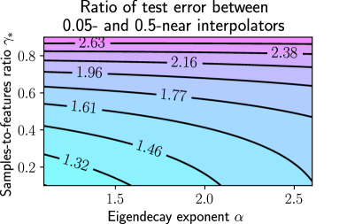
Figure 2: Larger power-law spectra exponent implies larger asymptotic excess test error when interpolating to $5\%$ of the noise compared to $50\%$ of the noise floor. Let $\mathcal{E}^{\ast}_{\mathtt{test}}=\mathcal{E}^{\ast}_{\mathtt{test}}(\alpha,\gamma_{\ast},\tau)$ be as in Theorem 1.5 where we make the dependency on parameters $\alpha,\gamma_{\ast},\tau$ explicit. The color and contour line of plot shows the ratio of test errors at two levels of nearness of interpolation $\mathcal{E}^{\ast}_{\mathtt{test}}(\alpha,\gamma_{\ast},0.05)/\mathcal{E}^{\ast}_{\mathtt{test}}(\alpha,\gamma_{\ast},0.5)$ over an $(\alpha,\gamma_{\ast})$-grid.

Using Proposition 3.2 with the implemenation of ${}_{2}F_{1}$ in SciPy, we illustrate the trade-off between the training error versus the test error in Figure 1-Right and the test error ratio in Figure 2.

Remark 3.3 (Data-independent regularizer-selection).

Let $\tau\in(0,\sigma^{2})$ be a desired level of nearness of interpolation. To select a regularizer $\varrho_{n}$ that achieves $\tau^{\prime}$-near-interpolation for $\tau^{\prime}\approx\tau$, we use the following method: Step 1. Find $k\in(k_{\mathtt{crit}},+\infty)$ such that $\mathcal{E}_{\mathtt{train}}^{*}=\mathcal{E}_{\mathtt{train}}^{*}(k)=\tau$, using the expression for $\mathcal{E}_{\mathtt{train}}^{*}(k)$ in Proposition 3.2. Let $k_{\tau}$ be such a $k$. Step 2. Next, set $r:=\mathcal{R}(k_{\tau})$, where $\mathcal{R}$ is also as in Proposition 3.2. Step 3. Set the regularizer as $\varrho_{n}:=rn^{\alpha}$.

4 RAPID NORM GROWTH

Proposition 1.7 can be proven in even greater generality under random matrix-theoretic assumptions.

Proposition 4.1 (Rapid norm growth under RMT).

Suppose Assumptions 2.2, 2.5, 2.6, and 2.9 all hold. For any $r>0$, let $\varrho_{n}:=rn^{-\alpha}$ be the regularizer for the ridge regression. Then $\mathbb{E}[\|\hat{\bm{\beta}}_{\varrho_{n}}\|_{2}^{2}]=\Omega(n^{\alpha})$.

The goal of this section is to sketch the proof for Proposition 4.1. Complete proofs of all results are included in the Appendix. Throughout, we assume the setting of Section 1.2.

The next step is the following:

Proposition 4.2.

Let $\varrho:=rn^{-\alpha}$. Then we have

$$\mathbb{E}\|\hat{\bm{\beta}}_{\varrho}\|_{2}^{2}\geq n^{\alpha}\sigma^{2}\cdot\mathbb{E}\big{[}\frac{d}{dr}(r\mathcal{S}_{\mathtt{esd}(n^{\alpha}\check{\mathbf{G}})}(-r))\big{]}.$$

The proof of Proposition 4.2 and other omitted proofs in this section can be found in Appendix B.

Given Proposition 4.2, the proof of Proposition 4.1 is straightforward:

Proof of Proposition 4.1.

Let

$$L:=\lim_{n\to\infty}\mathbb{E}\big{[}\tfrac{d}{dr}(r\mathcal{S}_{\mathtt{esd}(n^{\alpha}\check{\mathbf{G}})}(-r))\big{]}>0$$

be as in Assumption 2.9. Thus, for all $n\gg 0$ sufficiently large, we have $\mathbb{E}\big{[}\tfrac{d}{dr}(r\mathcal{S}_{\mathtt{esd}(n^{\alpha}\check{\mathbf{G}})}(-r))\big{]}>L/2>0$. By Proposition 4.2, we get that $\mathbb{E}\|\hat{\bm{\beta}}_{\varrho}\|_{2}^{2}\geq n^{\alpha}\sigma^{2}\cdot\frac{L}{2}$ for all $n\gg 0$, as desired. ∎

4.1 $\alpha$-scaled limiting spectral distribution

In this section, we check that power-law spectra covariance matrices has an $\alpha$-scaled limiting spectral distribution. In other words, Assumption 1.4 implies Assumption 2.2. Note that this is necessary because we have proved Proposition 4.1 rather than Proposition 1.7. So we need to make sure that the special case, i.e., Proposition 1.7, is indeed the “special case”.

Definition 4.3.

Given a measure $\mu$ on $\mathbb{R}$, we let $\mathtt{cdf}[\mu]$ denote the cumulative distribution function (CDF) of $\mu$.

Proposition 4.4.

Under Assumption 1.4, we have that Assumption 2.2 holds. In other words,

$$\lim_{n\to\infty}\mathtt{cdf}[\mathtt{esd}(n^{\alpha}\bm{\Sigma})](t)=\begin{cases}1-\gamma_{\ast}t^{-1/\alpha}&:t\geq\gamma_{\ast}^{\alpha}\\ 0&\mbox{otherwise.}\end{cases}$$

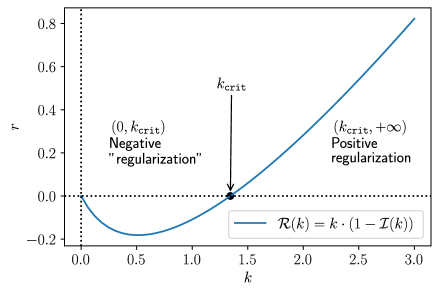
Figure 3: The $\mathcal{R}(k)$ function from Proposition 3.2. The $x$-axis is the input $k$. Note that for $k<k_{\mathtt{crit}}$ the regularizer $r$ is negative. Although we are only interested in the $(k_{\mathtt{crit}},+\infty)$ portion, negative regularizers have been studied by Tsigler and Bartlett, (2020); Wu and Xu, (2020).

4.2 Looseness of norm-based generalization bounds

Conjecturally, a norm-based generalization bound for near-interpolators should have the following form: under suitable assumptions, with high probability

$$\sup_{\bm{\beta}:\|\bm{\beta}\|\leq B,\mathcal{E}_{\mathtt{train}}(\bm{\beta})\leq\tau}\mathcal{E}_{\mathtt{test}}(\bm{\beta})=O\left(\frac{B^{2}\text{Tr}(\bm{\Sigma})}{n}\right).$$

where $\tau\in\mathbb{R}_{\geq 0}$. For $\tau=0$, the best known bound for (perfect) interpolators is given by Koehler et al., (2021, Corollary 1) under Gaussian assumption on the data $X\sim\mathcal{N}(0,\bm{\Sigma})$ and $B\geq\|\bm{\beta}^{\star}\|$.

To the best of our knowledge, there is no known extension to the case of near-interpolators, i.e., where $\tau>0$. However, such bound is not informative for our scenario, since by Theorem 1.5 and Proposition 1.7, it is possible to choose $\varrho_{n}$ such that 1. $\mathbb{E}[\mathcal{E}_{\mathtt{train}}(\hat{\bm{\beta}}_{\varrho_{n}})]\to\tau$, 2. $\mathcal{E}_{\mathtt{test}}(\hat{\bm{\beta}}_{\varrho_{n}})\to c\in\mathbb{R}_{\geq 0}$, and 3. $\|\bm{\beta}_{\varrho_{n}}\|^{2}=\Omega(n^{\alpha})$ for any $\alpha>0$. Thus, the bound goes to infinity while $\mathcal{E}_{\mathtt{test}}(\hat{\bm{\beta}}_{\varrho_{n}})$ is finite.

5 EXPERIMENTS

We run two types of synthetic experiments. The first type, plotted in Figure 1, employs (linear) ridge regression. The second type, plotted in Figure 4 employs neural networks. The data for both types of experiments are drawn from the HDA model (Example 2.8). Moreover, we have conducted experiments on several real world regression datasets from the UCI regression collection.

5.1 Experiments on synthetic data

To generate Figure 1-left, we run experiments with $\alpha\in\{1.25,2.5\}$ and $\tfrac{n}{p}=\gamma_{\ast}=\tfrac{2}{3}$. We sweep over the train MSE parameter $\mathcal{E}_{\mathtt{train}}^{*}$ to explore the trade-off between the train and testing MSE in linear ridge regression as described in Theorem 1.5. The value of $\mathcal{E}_{\mathtt{train}}^{*}$ are sweeped on a linearly-spaced grid of size $16$ from $0.05\sigma^{2}$ to $0.8\sigma^{2}$. The parameters are $n_{\mathtt{train}}=5000$, $n_{\mathtt{test}}=1000$, $\gamma_{\ast}=0.5$, $\alpha=1.75$ and $\sigma^{2}=1$.

The regularizer achieving a desired training MSE $\tau\in(0,\sigma^{2})$ is chosen according to the method described in Remark 3.3. We sample $\bm{\beta}^{\star}\in\mathbb{R}^{p}$ such that $\bm{\beta}^{\star}_{i}$ are i.i.d Gaussian with zero mean and variance $=10/p$.

The same set up is used for Figure 1-right, except we sweep over $n_{\mathtt{train}}$ rather than over $\mathcal{E}_{\mathtt{train}}^{*}$. The value of $n_{\mathtt{train}}$ are sweeped on a logarithmically-spaced grid of size $20$ from $200$ to $5000$.

For Figure 4, the identical set-up is used as in the Figure 1, except ridge regression is replaced with neural networks during training. We emphasize that the ground truth data (i.e., the teacher) is still generated via the same linear function $\bm{\beta}^{\star}$. All code for the experiments are included in Appendix E.

Remark 5.1.

As discussed in the introduction, near-interpolating neural network and its interpolation-generalization trade-offs exhibit similar phenomenon as in the case of ridge regression. Namely, larger power-law spectra exponent implies larger asymptotic excess test error when interpolating to $5\%$ of the noise compared to $50\%$ of the noise floor, for instance.

Remark 5.2.

Intriguely, in both the ridge regression (Figure 1) and neural network (Figure 4) experiments, the setting with to larger value of the norm-growth exponent $\alpha$ (right panels) results in poorer trade-offs (left panels). For ridge regression, this is explained by the “Moreover” part of Theorem 1.5. We believe it is an interesting future direction whether this behavior can be proved in the neural network setting.

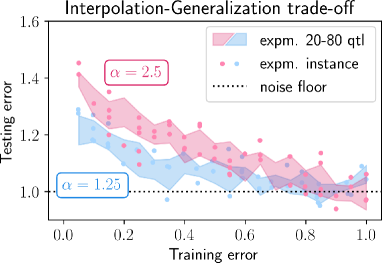
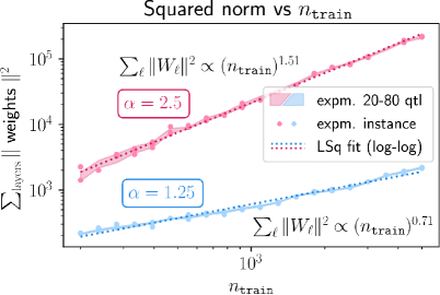
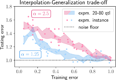
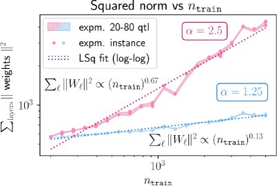
Figure 4: Experiments with neural networks (top row: 1-hidden layer, bottom row: 5-hidden layers). Analogous to Figure 1. See Section 5 and Remark 5.1 for details.

5.2 Experiments on UCI datasets

We conduct experiments on the forest and the stock datasets from the UCI regression collection (Kelly et al.,, 2023). Using neural tangent kernels (Arora et al.,, 2019), we observe power-law spectra in the kernel matrices for both of these datasets (Figure 5-right and Figure 6-right). In this subsection, we discuss the experiments on the forest dataset in relation to our theoretical results. Due to space constraints, we refer the reader to Appendix F for details of the experimental setup.

In Figure 5-left, note that the curve corresponding to forest.2-1 has the fastest spectra decay and simultaneously the worst trade-off. Evidently, larger decay exponent corresponds to a poorer trade-off, especially for near-interpolators, i.e., as the training error approaches $0$. This is in agreement with our theoretical results under random matrix theory assumptions illustrated in Figure 2. Similar phenomenon occurs for the stock dataset. See Appendix F.

6 ADDITIONAL RELATED WORKS AND NOVELTY OF OUR WORK

Technical Novelty of Theorem 1.7. Prior works of Hastie et al., (2022); Derezinski et al., (2019) require a lower bound on the smallest eigenvalue of the covariance matrix. Hence, the scenario studied in this paper is not amenable to their results. Further, Theorem 1.5 shows that when we have a sharper decay (larger $\alpha$) of the eigenvalues, we have a worse tradeoff between the test and training error. Hence, we show that the scenario from Hastie et al., (2022) is the most benign one. This well conditioning assumption is relaxed in Cheng and Montanari, (2022), however, they require that $\|\Sigma^{-1/2}\beta\|$ is finite. We do not require this assumption. Finally, Dobriban and Wager, (2018) does not need the well-conditioning assumption but instead needs to assume an isotropic distribution on $\beta$. Since we work with fixed $\beta$, their results do not apply.

Trade-offs in interpolation-based learning. Prior works (Ghosh and Belkin,, 2022; Belkin et al.,, 2018; Sonthalia et al.,, 2023) have studied the tradeoff between near interpolation and generalization. For regression, previous works have also studied the fundamental trade-off in learning algorithms between overparametrization and (Lipschitz) smoothness (Bubeck and Sellke,, 2021), and robustness and smoothness (Zhang et al.,, 2022).

Loosenss of existing generalization bounds. Belkin et al., (2018, Theorem 1) establishes for classification that the RKHS norm of a “near-interpolating” classifier grows at rate $\Omega(\exp(n^{1/p}))$. The growth is unbounded if $n=\Omega(\exp(p))$. If the number of samples $n=\Theta(\mathrm{poly}(p))$, then the lower bound does not grow to infinity. While our results are for regression and thus not directly comparable, our lower bound is meaningful in the more practical $n\propto p$ regime.

Power-law spectra datasets. Synthetic data with artificial power law EVD covariance have been used frequently as toy examples (Berthier et al.,, 2020; Mallinar et al.,, 2022). On real datasets, power law EVD is often observed to describe neural tangent kernels (NTK) well in practice, including on MNIST ((Bahri et al.,, 2021, Fig, 4) and (Velikanov and Yarotsky,, 2022, Fig. 2)), Fashion-MNIST (Cui et al.,, 2021, Fig. 7) Caltech 101 (Murray et al.,, 2022, Fig. 1), CIFAR-100 (Wei et al.,, 2022, Fig. 3).

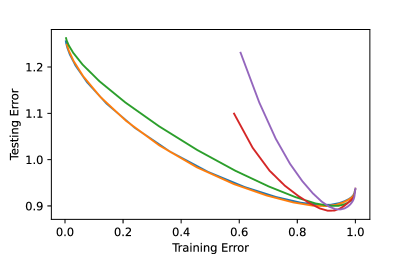
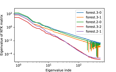
Figure 5: Left. Training/testing error trade-off on the “forest” dataset from the UCI regression dataset collection using kernel ridge regression with the neural tangent kernel. Each curve is labeled by “DatasetName.d-f” where “d” and “f” represents the number of layers and the number of fixed layers in the NTK corresponding to ReLU networks. Right. The eigenvalue index vs eigenvalue plot of the NTK matrix exhibits power-law spectra. A tiny value is added to the eigenvalues for better visualization on the log-scale.

Theoretical machine learning works using power-law spectra. Bordelon et al., (2020) shows that power law EVD implies power law learning curve. Velikanov and Yarotsky, (2021, §6.2) computes the power law EVD exponent for certain NTKs with ReLU to be $\alpha=1+\frac{1}{d}$. Murray et al., (2022) computes the EVD for NTKs with several different activations. Bartlett et al., (2020, Theorem 6) shows that benign overfitting occurs when the covariance matrix eigenvalues $\lambda_{i}=i^{-1}\log^{-b}(i+1)$ for $b>1$. Mallinar et al., (2022) studies power law decay for $\alpha\geq 1$ and proposes a taxonomy of overfitting into three categories: catastropic, tempered and benign. The EVD condition is also known as the capacity condition in the kernel ridge regression literature. See Bietti et al., (2021) and the references there-in.

Random matrix theory (RMT). The signal processing research community have long been using RMT for theoretical analysis (Couillet and Debbah,, 2012). Increasingly RMT has been applied to machine learning as well as a key tool for analysis.

In particular, Dobriban and Wager, (2018); Hastie et al., (2022); Jacot et al., 2020b ; Liang and Rakhlin, (2020) have applied RMT for (kernel) ridge regression, Sonthalia and Nadakuditi, (2023); Kausik et al., (2023) use it to understand generalization of linear denoisers, Paquette et al., (2022, 2021) uses the so-called local Marchenko-Pastur law (Knowles and Yin,, 2017) to analyze gradient-based algorithms. Finally, Wei et al., (2022) also applies such local law to analyze the so-called generalized cross- validation (GCV) estimator.

7 DISCUSSION AND LIMITATIONS

We conclude with several future research directions that we believe will be fruitful:

Connection to early stopping. Typically, early stopping prevents the trained algorithm from perfectly interpolating the data. Can early stopped learning theory results, e.g., Ji et al., (2021); Kuzborskij and Szepesvári, (2022), be applied to analyze near-interpolators?

Near-interpolators and uniform convergence generalization bound. Is possible to use uniform convergence-based approach to give non-vacuous generalization bound under the setting studied in this work? This question has already been raised by Dobriban and Wager, (2018) in the context of classification in a similar setting. An interesting question is if classical learning theory can be used to obtain results that are currently only obtained via random matrix theoretic or similar techniques. Another approach is to extend the results of Koehler et al., (2021) to the near-interpolation setting.

Limitations. Our work is restricted to analyzing a random matrix model. Understanding the phenomenon uncovered in this paper in more general models and additional real world settings will be needed. Moreover, our work does not rule out the existence of uniform convergence generalization bound.

Code availability. Code used to run and plot the experiments shown in all figures is available at https://github.com/YutongWangUMich/Near-Interpolators-Figures.

Acknowledgements

YW acknowledges support from the Eric and Wendy Schmidt AI in Science Postdoctoral Fellowship, a Schmidt Futures program. WH acknowledges support from the Google Research Scholar program.

Checklist

1. For all models and algorithms presented, check if you include:

   1. A clear description of the mathematical setting, assumptions, algorithm, and/or model. [Yes]

   2. An analysis of the properties and complexity (time, space, sample size) of any algorithm. [Not Applicable]

   3. (Optional) Anonymized source code, with specification of all dependencies, including external libraries. [Yes]

2. For any theoretical claim, check if you include:

   1. Statements of the full set of assumptions of all theoretical results. [Yes]

   2. Complete proofs of all theoretical results. [Yes]

   3. Clear explanations of any assumptions. [Yes]

3. For all figures and tables that present empirical results, check if you include:

   1. The code, data, and instructions needed to reproduce the main experimental results (either in the supplemental material or as a URL). [Yes]

   2. All the training details (e.g., data splits, hyperparameters, how they were chosen). [Yes]

   3. A clear definition of the specific measure or statistics and error bars (e.g., with respect to the random seed after running experiments multiple times). [Yes]

   4. A description of the computing infrastructure used. (e.g., type of GPUs, internal cluster, or cloud provider). [Yes]

4. If you are using existing assets (e.g., code, data, models) or curating/releasing new assets, check if you include:

   1. Citations of the creator If your work uses existing assets. [Not Applicable]

   2. The license information of the assets, if applicable. [Not Applicable]

   3. New assets either in the supplemental material or as a URL, if applicable. [Not Applicable]

   4. Information about consent from data providers/curators. [Not Applicable]

   5. Discussion of sensible content if applicable, e.g., personally identifiable information or offensive content. [Not Applicable]

5. If you used crowdsourcing or conducted research with human subjects, check if you include:

   1. The full text of instructions given to participants and screenshots. [Not Applicable]

   2. Descriptions of potential participant risks, with links to Institutional Review Board (IRB) approvals if applicable. [Not Applicable]

   3. The estimated hourly wage paid to participants and the total amount spent on participant compensation. [Not Applicable]

Appendix

Appendix A Proof of Theorem 1.5 — the exact trade-off formula

Our goal is to calculate the asymptotic test error $\mathcal{E}_{\mathtt{test}}^{\ast}$ under the assumptions of Theorem 1.5. This is accomplished through the following three steps.

The first step is to calculate the closed-form solution for the integrals defined in Definition 3.1 which are key ingredients for the expression of $\mathcal{E}_{\mathtt{test}}^{\ast}$. This is done in Section A.1. The second step is to relate the integrals from Definition 3.1 to the self-consistent equations in Equation 6. This is done in Section A.2. The final step is to relate the self-consistent equations Equation 6 to the asymptotic test error $\mathcal{E}_{\mathtt{test}}^{\ast}$. This is done in Section A.3.

A.1 Closed-form expression for the integrals in Definition 3.1

We prove the identities

$$\int_{0}^{\tfrac{1}{\gamma_{\ast}}}\frac{dx}{1+k{x}^{\alpha}}=\gamma_{\ast}^{-1}F(1,\tfrac{1}{\alpha};1+\tfrac{1}{\alpha};-k\gamma_{\ast}^{-\alpha}),\,\,\mbox{and}$$

$$\int_{0}^{\tfrac{1}{\gamma_{\ast}}}\frac{dx}{(1+k{x}^{\alpha})^{2}}=\gamma_{\ast}^{-1}F(2,\tfrac{1}{\alpha};1+\tfrac{1}{\alpha};-k\gamma_{\ast}^{-\alpha}).$$

as shown in the main text following Definition 3.1.

Proof.

Let ${}_{2}F_{1}(a,b;c;z)$ be the Gauss hypergeometric function. Note that the function can be implemented in SciPy as scipy.special.hyp2f1 and is used to plot Figure 1. Let $\Gamma$ denote the Gamma function. The integral representation of the Gaussian hypergeometric function is well-known and is given by

$${}_{2}F_{1}(\sigma,a;b;-z)=\frac{\Gamma(b)}{\Gamma(a)\Gamma(b-a)}\int_{0}^{1}\frac{t^{a-1}(1-t)^{b-a-1}}{(1+zt)^{\sigma}}dt.$$ (7)

Moreover, (7) is finite for $z\in\mathbb{C}\setminus(-\infty,-1]$ and $\Re(b-a)>0$ and $\Re(a)>0$. Thus, by Equation 7, we have

$${}_{2}F_{1}(1,\tfrac{1}{\alpha};1+\tfrac{1}{\alpha};-k\gamma_{\ast}^{-\alpha})=\frac{\Gamma(1+\tfrac{1}{\alpha})}{\Gamma(\tfrac{1}{\alpha})\Gamma(1)}\int_{0}^{1}\frac{t^{1/\alpha}t^{-1}}{1+k\gamma_{\ast}^{-\alpha}t}dt=\frac{1}{\alpha}\int_{0}^{1}\frac{t^{1/\alpha}t^{-1}}{1+k\gamma_{\ast}^{-\alpha}t}dt$$

where the second inequality follows from the well-known identity $z=\Gamma(1+z)/\Gamma(z)$ for the Gamma function. Let $u=t^{1/\alpha}$. Then we have $du=\frac{1}{\alpha}t^{1/\alpha}t^{-1}dt$. Thus, by u-substitution, we have

$$\frac{1}{\alpha}\int_{0}^{1}\frac{t^{1/\alpha}t^{-1}}{1+k\gamma_{\ast}^{-\alpha}t}dt=\int_{0}^{1}\frac{1}{1+k\gamma_{\ast}^{-\alpha}u^{\alpha}}du=\int_{0}^{1/\gamma_{\ast}}\frac{\gamma_{\ast}}{1+kx^{\alpha}}dx$$

where the second inequality used u-substituted with $x=u/\gamma_{\ast}$. Now, we have by the definition of $\mathcal{I}$ in Definition 3.1 that

$$\mathcal{I}(k)=\int_{0}^{1/\gamma_{\ast}}\frac{1}{1+kx^{\alpha}}dx=\frac{1}{\gamma_{\ast}}\int_{0}^{1/\gamma_{\ast}}\frac{\gamma_{\ast}}{1+kx^{\alpha}}dx=\frac{1}{\gamma_{\ast}}{}_{2}F_{1}(1,\tfrac{1}{\alpha};1+\tfrac{1}{\alpha};-k\gamma_{\ast}^{-\alpha})$$

as desired. By an analogous calculation, we get $\mathcal{J}(k)=\frac{1}{\gamma_{\ast}}{}_{2}F_{1}(2,\tfrac{1}{\alpha};1+\tfrac{1}{\alpha};-k\gamma_{\ast}^{-\alpha})$. ∎

A.2 Proof of Proposition 3.2

We begin by analyzing the functions defined in Definition 3.1 and prove the items 1 and 2 of the “Moreover” part of Proposition 3.2:

Proposition A.1.

Let $\mathcal{I}$ and $\mathcal{J}$ be functions as defined in Definition 3.1. Under Assumption 1.4 and Assumption 2.5, we have that $r=\mathcal{R}(k):=k\cdot(1-\mathcal{I}(k))$ and $\tfrac{dr}{dk}=1-\mathcal{J}(k)$.

Furthermore, the following holds:

1. $\mathcal{R}(k)\asymp k$ for $k\gg 0$,

2. There exists $k_{\mathtt{crit}}>0$ such that $\mathcal{R}(k_{\mathtt{crit}})=0$, $\mathcal{R}$ is increasing and positive on $(k_{\mathtt{crit}},+\infty)$.

3. $\mathcal{J}(k)<1$ for $k\in(k_{\mathtt{crit}},+\infty)$ and $\mathcal{J}(+\infty)=0$.

Proof of Proposition A.1.

We begin by proving the first part: that $r=\mathcal{R}(k):=k\cdot(1-\mathcal{I}(k))$ and $\tfrac{dr}{dk}=1-\mathcal{J}(k)$. Rewrite the limit in Equation 6 as follows:

$$\lim_{n\to\infty}\frac{1}{n}\sum_{i=1}^{p}\frac{1}{1+kn^{-\alpha}\lambda_{i}^{-1}}=\lim_{n\to\infty}\frac{1}{n}\sum_{i=1}^{n/\gamma}\frac{1}{1+k{(i/n)}^{\alpha}}=\int_{0}^{1/\gamma_{\ast}}\frac{dx}{1+k{x}^{\alpha}}$$

The right-most equality follows from the definition of the (Riemann) integral. If $\gamma_{\ast}=0$, then $1/\gamma_{\ast}=+\infty$ and the above is interpreted as an improper Riemann integral. Now, rearranging Equation 6, we get the desired formula of $r=\mathcal{R}(k):=k\cdot(1-\mathcal{I}(k))$. The formula for $\frac{dr}{dk}$ follows by “differentiating under the integral” (Leibniz integral rule).

For the first item of the “Furthermore” part, it suffices to show that $\lim_{k\to+\infty}\mathcal{I}(k)=0$. This follows from the fact that $\lim_{k\to+\infty}\frac{1}{1+kx^{\alpha}}=0$ for all $x>0$, integrability of the function $(1+x^{\alpha})^{-1}$ over $\mathbb{R}_{\geq 0}$, and the dominated convergence theorem. Likewise, $\lim_{k\to\infty}\mathcal{J}(k)=0$ as well.

For the second item of the “Furthermore” part, we note that for all $x$ sufficiently large, we have $\tfrac{dr}{dk}>0$ since $\lim_{k\to\infty}\mathcal{J}(k)=0$. Now, let $k_{\mathtt{crit}}$ be the largest real number such that $\mathcal{R}(k_{\mathtt{crit}})=0$. Since $\mathcal{R}(0)=0$, we must have $k_{\mathtt{crit}}\geq 0$.

For all $k>k_{\mathtt{crit}}$, we claim that $\mathcal{I}(k)<1$. To see this, assume the contrary. Then by the fact that $\lim_{k\to+\infty}\mathcal{I}(k)=0$ and the intermediate value theorem, there must exists $k^{\prime}$ such that $k^{\prime}>k$ such that $\mathcal{I}(k^{\prime})=1$ which implies that $\mathcal{R}(k^{\prime})=0$. This contradicts the maximality of $k_{\mathtt{crit}}$.

Finally, since $1+kx^{\alpha}\leq(1+kx^{\alpha})^{2}$ for all $k\geq 0$ and $x\geq 0$, we have that $\mathcal{I}(k)\geq\mathcal{J}(k)$ for all such $k$’s. Thus, by the previous claim, for all $k>k_{\mathtt{crit}}$, we have $1>\mathcal{I}(k)\geq\mathcal{J}(k)$. This proves that $\frac{dr}{dk}>0$ for all $k>k_{\mathtt{crit}}$, as desired. ∎

A.3 Review of the eigenlearning framework (Simon et al.,, 2023)

Before proceeding with finishing the proof of Proposition 3.2, we briefly review the eigenlearning framework. Simon et al., (2023) calculates the test error for the estimator

$$\check{\bm{\beta}}_{\delta}:=\mathbf{X}(\mathbf{X}^{\top}\mathbf{X}+\delta\mathbf{I}_{n})^{-1}y=\mathbf{X}(n\check{\mathbf{G}}+\delta\mathbf{I}_{n})^{-1}y$$ (8)

for kernel ridge regression using the so-called eigenlearning equations (Simon et al.,, 2023, Section 4.1). Below, we recall some relevant parts of the framework:

Definition A.2 (Eigenlearning eqn. specialized to setting in Section 1.3).

Suppose that the ground truth regression function is linear, i.e., $f(x)=x^{\top}\bm{\beta}^{\star}$ for some $\bm{\beta}^{\star}\in\mathbb{R}^{p}$. Let $\delta$ and $\kappa$ satisfy the equation

$$n=\frac{\delta}{\kappa}+\sum_{i=1}^{p}\frac{\lambda_{i}}{\lambda_{i}+\kappa}.$$ (9)

Define the following $n$-dependent quantities:

1. Overfitting coefficient: $\mathcal{E}_{\mathtt{coef}}:=n\frac{d\kappa}{d\delta}$

2. Testing error: $\mathcal{E}_{\mathtt{test}}:=\mathcal{E}_{\mathtt{coef}}(\sigma^{2}+C)$ where

   $$C=\textstyle\sum_{i=1}^{p}(1-\mathcal{L}_{i})(\beta^{\star}_{i})^{2}\quad\mbox{and}\quad\mathcal{L}_{i}:=\frac{\lambda_{i}}{\lambda_{i}+\kappa}.$$

3. Training error: $\mathcal{E}_{\mathtt{train}}:=\frac{\delta^{2}}{n^{2}\kappa^{2}}\mathcal{E}_{\mathtt{test}}$.

Proof of Proposition 3.2.

Simon et al., (2023) uses a different scaling for ridge regression than the one we use. To bridge the different notations, we first resolve this discrepancy. Comparing Equation 8 with the expression in Equation 11, if we let $\delta:=n\varrho$, then the expressions are equivalent, i.e., $\check{\beta}_{\delta}=\hat{\beta}_{\varrho}$. To see this, note that

$$\check{\beta}_{\delta}=\check{\beta}_{n\varrho} =X(X^{\top}X+n\varrho\mathbb{I}_{n})^{-1}y$$

$$=(XX^{\top}+n\varrho\mathbb{I}_{p})^{-1}Xy\quad\because\mbox{\lx@cref{creftypecap~refnum}{lemma:woodbury}}$$

$$=(n(n^{-1}XX^{\top}+\varrho\mathbb{I}_{p}))^{-1}Xy$$

$$=(\hat{\Sigma}+\varrho\mathbb{I}_{p})^{-1}\tfrac{1}{n}Xy=\hat{\beta}_{\varrho}\quad\because{\mbox{Definition of $\hat{\beta}_{\varrho}$}}$$

Below, let $r>0$ be arbitrary. Furthermore, we claim that as ${n\to\infty}$, we have $r,k$ satisfies Equation 6 if and only if the tuple $(\delta,\kappa):=(nrn^{-\alpha},kn^{-\alpha})$ satisfies Equation 9:

$$n=\frac{\delta}{\kappa}+\sum_{i=1}^{p}\frac{\lambda_{i}}{\lambda_{i}+\kappa}\iff n=\frac{nrn^{-\alpha}}{kn^{-\alpha}}+\sum_{i=1}^{p}\frac{\lambda_{i}}{\lambda_{i}+kn^{-\alpha}}\iff 1=\frac{r}{k}+\frac{1}{n}\sum_{i=1}^{p}\frac{1}{1+kn^{-\alpha}\lambda_{i}^{-1}}.$$

Taking limit as $n\to\infty$, we have proved the claim.

Next, we show that $\lim_{n\to\infty}C=0$ where $C$ is as in Definition A.2. We have $\mathcal{L}_{i}:=\frac{\lambda_{i}}{\lambda_{i}+\kappa}=\frac{1}{1+k(i/n)^{\alpha}}$. Note that $\lim_{n\to\infty}\mathcal{L}_{i}=1$ for all fixed $i$. On the other hand, since $\sup_{n=1,2\dots}\|\beta^{\star}\|_{2}<+\infty$, dominated convergence theorem implies that $\lim_{n\to\infty}C=0$

We claim that the following asymptotic expression for the testing and training error hold:

$$\lim_{n\to\infty}\mathcal{E}_{\mathtt{test}}=\sigma^{2}\cdot\tfrac{dk}{dr}\quad\mbox{and}\quad\lim_{n\to\infty}\mathcal{E}_{\mathtt{train}}=\sigma^{2}\cdot\tfrac{r^{2}}{k^{2}}\cdot\tfrac{dk}{dr}$$ (10)

where $r$ and $k$ satisfy Equation 6 from from Assumption 2.5.

To see this, first note that the overfitting coefficient satisfies

$$\mathcal{E}_{\mathtt{coef}}:=n\tfrac{d\kappa}{d\delta}=n\tfrac{d\kappa}{d\varrho}\tfrac{d\varrho}{d\delta}=n\tfrac{d\kappa}{d\varrho}\tfrac{1}{n}=\tfrac{d\kappa}{d\varrho}=\tfrac{dk}{dr}.$$

Thus, we obtain the following asymptotic expression

$$\lim_{n\to\infty}\mathcal{E}_{\mathtt{test}}=\mathcal{E}_{\mathtt{coef}}\cdot\sigma^{2}=\sigma^{2}\cdot\tfrac{dk}{dr}.$$

On the other hand, the training error is given by

$$\mathcal{E}_{\mathtt{train}}=\tfrac{\delta^{2}}{n^{2}\kappa^{2}}\mathcal{E}_{\mathtt{test}}=\tfrac{\varrho^{2}}{\kappa^{2}}\mathcal{E}_{\mathtt{test}}=\mathcal{E}_{\mathtt{test}}\cdot\tfrac{r^{2}}{k^{2}}.$$

Therefore, $\lim_{n\to\infty}\mathcal{E}_{\mathtt{train}}=\sigma^{2}\cdot\tfrac{r^{2}}{k^{2}}\cdot\tfrac{dk}{dr}$. This proves (10), as desired. ∎

Appendix B Proof of Proposition 4.1 — rapid norm growth under RMT assumptions

The first key technical step the following:

Proposition B.1.

$\mathbb{E}\|\hat{\bm{\beta}}_{\varrho}\|_{2}^{2}\geq n^{-1}\sigma^{2}\mathbb{E}[\mathrm{tr}((\hat{\bm{\Sigma}}+\varrho\mathbf{I}_{p})^{-2}\hat{\bm{\Sigma}})]$.

Proof.

Below, for brevity we let $\mathbf{a}:=\mathbf{X}^{\top}\bm{\beta}^{\star}$ and $\mathbf{M}:=(\hat{\bm{\Sigma}}+\varrho\mathbf{I}_{p})^{-1}\frac{1}{n}\mathbf{X}$. Recall the closed-form solution for Equation 2 is given by the formula

$$\hat{\bm{\beta}}_{\varrho}:=(\hat{\bm{\Sigma}}+\varrho\mathbf{I}_{p})^{-1}\tfrac{1}{n}\mathbf{X}y.$$ (11)

Thus,

$$\hat{\bm{\beta}}_{\varrho}=(\hat{\bm{\Sigma}}+\varrho\mathbf{I}_{p})^{-1}\frac{1}{n}\mathbf{X}y=(\hat{\bm{\Sigma}}+\varrho\mathbf{I}_{p})^{-1}\frac{1}{n}\mathbf{X}(f(\mathbf{X})+{\bm{\varepsilon}})=\mathbf{M}(\mathbf{a}+\bm{\varepsilon}).$$

Thus,

$$\|\hat{\bm{\beta}}_{\varrho}\|_{2}^{2}=(\mathbf{a}+\bm{\varepsilon})^{\top}\mathbf{M}^{\top}\mathbf{M}(\mathbf{a}+\bm{\varepsilon})=\underbrace{\mathbf{a}^{\top}\mathbf{M}^{\top}\mathbf{M}\mathbf{a}}_{\geq 0}+\bm{\varepsilon}^{\top}\mathbf{M}^{\top}\mathbf{M}\bm{\varepsilon}+2\bm{\varepsilon}^{\top}\mathbf{M}^{\top}\mathbf{M}\mathbf{a}.$$

Note that $\bm{\varepsilon}\perp\mathbf{M}^{\top}\mathbf{M}\mathbf{a}$ since $\bm{\varepsilon}\perp\mathbf{X}$. Thus, since $\mathbb{E}[\bm{\varepsilon}]=0$, we have

$$\mathbb{E}[\|\hat{\bm{\beta}}_{\varrho}\|_{2}^{2}]=\mathbb{E}[(\mathbf{a}+\bm{\varepsilon})^{\top}\mathbf{M}^{\top}\mathbf{M}(\mathbf{a}+\bm{\varepsilon})]\geq\mathbb{E}[\bm{\varepsilon}^{\top}\mathbf{M}^{\top}\mathbf{M}\bm{\varepsilon}]=\mathbb{E}[\mathrm{tr}(\mathbf{M}^{\top}\mathbf{M}\bm{\varepsilon}\bm{\varepsilon}^{\top})].$$

Since $\mathbf{M}^{\top}\mathbf{M}\perp\bm{\varepsilon}\bm{\varepsilon}^{\top}$, we have

$$\mathbb{E}[\mathrm{tr}(\mathbf{M}^{\top}\mathbf{M}\bm{\varepsilon}\bm{\varepsilon}^{\top})]=\mathrm{tr}(\mathbb{E}[\mathbf{M}^{\top}\mathbf{M}]\mathbb{E}[\bm{\varepsilon}\bm{\varepsilon}^{\top}])=\mathrm{tr}(\mathbb{E}[\mathbf{M}^{\top}\mathbf{M}\sigma^{2}\mathbf{I}_{n}])=\sigma^{2}\mathbb{E}[\mathrm{tr}(\mathbf{M}^{\top}\mathbf{M})].$$

On the other hand, $\mathbf{M}^{\top}\mathbf{M}=\frac{1}{n}(\hat{\bm{\Sigma}}+\varrho\mathbf{I}_{p})^{-1}\hat{\bm{\Sigma}}(\hat{\bm{\Sigma}}+\varrho\mathbf{I}_{p})^{-1}$. Using the cyclic property of trace, we get the desired inequality. ∎

Proof sketch of Prop. B.1.

We first simplify $\|\hat{\bm{\beta}}_{\varrho}\|_{2}^{2}$ using the well-known formula for ridge regression: Next, let $\mathbf{M}:=(\hat{\bm{\Sigma}}+\varrho\mathbf{I}_{p})^{-1}\tfrac{1}{n}\mathbf{X}$. Using the independence of $\mathbf{X}$ and $\bm{\varepsilon}$, we get $\mathbb{E}[\|\hat{\bm{\beta}}_{\varrho}\|_{2}^{2}]\geq\mathbb{E}[\mathrm{tr}(\mathbf{M}^{\top}\mathbf{M}\bm{\varepsilon}\bm{\varepsilon}^{\top})]$. Since $\mathbf{M}^{\top}\mathbf{M}$ and $\bm{\varepsilon}\bm{\varepsilon}^{\top}$ are also independent, we have

$$\mathbb{E}[\mathrm{tr}(\mathbf{M}^{\top}\mathbf{M}\bm{\varepsilon}\bm{\varepsilon}^{\top})]=\sigma^{2}\mathbb{E}[\mathrm{tr}(\mathbf{M}^{\top}\mathbf{M})].$$

By $\mathbf{M}^{\top}\mathbf{M}=\frac{1}{n}(\hat{\bm{\Sigma}}+\varrho\mathbf{I}_{p})^{-1}\hat{\bm{\Sigma}}(\hat{\bm{\Sigma}}+\varrho\mathbf{I}_{p})^{-1}$ and the cyclic property of trace, we get the desired inequality. ∎

For the sake of completeness, we prove Equation 11 though its well-known

Proof of Equation 11.

Start with the objective function $\mathcal{F}(\bm{\beta}):=\frac{1}{n}\|\mathbf{X}^{\top}\bm{\beta}-\mathbf{y}\|_{2}^{2}+\varrho\|\bm{\beta}\|_{2}^{2}$. Take derivative with respect to $\bm{\beta}$, we have

$$\frac{1}{2}\nabla_{\bm{\beta}}\left(\frac{1}{n}\|\mathbf{X}^{\top}\bm{\beta}-\mathbf{y}\|_{2}^{2}+\varrho\|\bm{\beta}\|_{2}^{2}\right)=\frac{1}{2}\nabla_{\bm{\beta}}\left(\bm{\beta}^{\top}(\hat{\bm{\Sigma}}+\varrho\mathbf{I}_{p})\bm{\beta}-\frac{2}{n}\bm{\beta}^{\top}\mathbf{X}\mathbf{y}\right)$$

$$=(\hat{\bm{\Sigma}}+\varrho\mathbf{I}_{p})\bm{\beta}-\frac{1}{n}\mathbf{X}\mathbf{y}.$$

Since $\nabla_{\bm{\beta}}\mathcal{F}(\hat{\bm{\beta}}_{\varrho})=0$, we are done. ∎

Lemma B.2 (Special case of Woodbury formula).

Let

$$\mathbf{M}\in\mathbb{R}^{p\times n}$$ (12)

be an arbitrary matrix and $\varrho\in(0,\infty)$. Then

$$(\mathbf{M}\mathbf{M}^{\top}+\varrho\mathbf{I}_{p})^{-1}\mathbf{M}=\mathbf{M}(\mathbf{M}^{\top}\mathbf{M}+\varrho\mathbf{I}_{n})^{-1}\in\mathbb{R}^{n\times p}.$$

Proof of Lemma B.2.

It suffices to prove Lemma B.2 for the special case when $\varrho=1$, which we assume below. By the Woodbury matrix identity, we have

$$(\mathbf{M}\mathbf{M}^{\top}+\mathbf{I}_{p})^{-1}=\mathbf{I}-\mathbf{M}(\mathbf{M}^{\top}\mathbf{M}+\mathbf{I}_{n})^{-1}\mathbf{M}^{\top}$$ (13)

For brevity, let $\mathbf{P}:=\mathbf{M}\mathbf{M}^{\top}+\mathbf{I}_{p}$ and let $\mathbf{N}:=\mathbf{M}^{\top}\mathbf{M}+\mathbf{I}_{n}$. To proceed, we have

$$\mathbf{P}^{-1}\mathbf{M}$$

$$=\mathbf{M}-\mathbf{M}\mathbf{N}^{-1}\mathbf{M}^{\top}\mathbf{M}\quad\because\mbox{Multiplying \eqref{equation:lemma:woodbury-1} by $\mathbf{M}$ on the right}$$

$$=\mathbf{M}(\mathbf{I}_{n}-\mathbf{N}^{-1}\mathbf{M}^{\top}\mathbf{M})\quad\because\mbox{Factoring out $\mathbf{M}$ on the left}$$

$$=\mathbf{M}(\mathbf{I}_{n}-(\mathbf{I}_{n}-\mathbf{N}^{-1}))\quad\because\mbox{$\mathbf{I}_{n}=\mathbf{N}^{-1}\mathbf{N}=\mathbf{N}^{-1}+\mathbf{N}^{-1}\mathbf{M}^{\top}\mathbf{M}$}$$

$$=\mathbf{M}\mathbf{N}^{-1}$$

as desired. ∎

Lemma B.3.

Let $\mathbf{M}\in\mathbb{R}^{p\times p}$ be any symmetric matrix and $z\in\mathbb{R}$. Then we have

$$\tfrac{d}{dz}\mathrm{tr}(z(\mathbf{M}+z\mathbf{I}_{p})^{-1})=\mathrm{tr}(\mathbf{M}(\mathbf{M}+z\mathbf{I}_{p})^{-2}).$$

Proof of Lemma B.3.

Without the loss of generality, suppose that $\mathbf{M}=\mathrm{diag}(\lambda_{i},\dots,\lambda_{p})$. Then we have $f(z):=\mathrm{tr}(z(\mathbf{M}+z\mathbf{I}_{p})^{-1})=\sum_{i=1}^{p}\frac{z}{\lambda_{i}+z}.$ Now, from elementary calculus, we have

$$\frac{d}{dx}\frac{x}{y+x}=(y+x)^{-1}-x(y+x)^{-2}=(y+x)^{-2}((y+x)-x)=\frac{y}{(y+x)^{2}}.$$

From this, we recover the fact that $\frac{d}{dz}f(z)=\sum_{i=1}^{n}\frac{\lambda_{i}}{(\lambda_{i}+z)^{2}}=\mathrm{tr}(\mathbf{M}(\mathbf{M}+z\mathbf{I}_{p})^{-2}),$ as desired. ∎

Lemma B.4 (Gram-to-covariance).

Let $c\in\mathbb{R}$ and $z\in\mathbb{C}$ be arbitrary, then $\mathcal{S}_{\mathtt{esd}(c\hat{\bm{\Sigma}})}(z)=\gamma\cdot\mathcal{S}_{\mathtt{esd}(c\check{\mathbf{G}})}(z)-\frac{(1-\gamma)}{z}$.

Proof of Lemma B.4.

Without the loss of generality, we may assume that $c=1$. Let $\hat{\lambda}_{1}\geq\dots\geq\hat{\lambda}_{p}$ be the eigenvalues of $\hat{\bm{\Sigma}}$. Since $p>n$, we necessarily have that $\hat{\lambda}_{n+1}=\cdots=\hat{\lambda}_{p}=0$. Moreover, $\hat{\lambda}_{1},\dots,\hat{\lambda}_{n}$ are the eigenvalues of $\check{\mathbf{G}}$. Now, unwinding the definition, we have

$$\mathcal{S}_{\mathtt{esd}(\hat{\bm{\Sigma}})}(z)=\frac{1}{p}\sum_{i=1}^{p}\frac{1}{\hat{\lambda}_{i}-z}$$

and

$$\mathcal{S}_{\mathtt{esd}(\check{\mathbf{G}})}(z)=\frac{1}{n}\sum_{i=1}^{n}\frac{1}{\hat{\lambda}_{i}-z}.$$

Thus,

$$\mathcal{S}_{\mathtt{esd}(\hat{\bm{\Sigma}})}(z) =\frac{1}{p}\left(\sum_{i=1}^{n}\frac{1}{\hat{\lambda}_{i}-z}+\sum_{i=n+1}^{p}\frac{1}{-z}\right)$$

$$=\left(\frac{n}{p}\frac{1}{n}\sum_{i=1}^{n}\frac{1}{\hat{\lambda}_{i}-z}\right)-\frac{p-n}{p}\frac{1}{z}$$

$$=\gamma\cdot\mathcal{S}_{\mathtt{esd}(\check{\mathbf{G}})}(z)-\frac{(1-\gamma)}{z}$$

as desired. ∎

Proof of Proposition 4.2.

Recall from Proposition B.1 that $\mathbb{E}\|\hat{\bm{\beta}}\|_{2}^{2}\geq n^{-1}\sigma^{2}\mathbb{E}[\mathrm{tr}((\hat{\bm{\Sigma}}+\varrho\mathbf{I}_{p})^{-2}\hat{\bm{\Sigma}})]$. Below, we analyze the term inside the expectation. By the definition of the Stieltjes transform, we have

$$\mathrm{tr}(\varrho(\hat{\bm{\Sigma}}+\varrho\mathbf{I}_{p})^{-1})=\mathrm{tr}(rn^{-\alpha}(\hat{\bm{\Sigma}}+rn^{-\alpha}\mathbf{I}_{p})^{-1})=\mathrm{tr}(r(n^{\alpha}\hat{\bm{\Sigma}}+r\mathbf{I}_{p})^{-1})=pr\mathcal{S}_{\mathtt{esd}(n^{\alpha}\hat{\bm{\Sigma}})}(-r).$$

Therefore, by Lemma B.3, we have

$$\frac{d}{dr}\left(pr\mathcal{S}_{\mathtt{esd}(n^{\alpha}\hat{\bm{\Sigma}})}(-r)\right)=\frac{d}{dr}\mathrm{tr}(\varrho(\hat{\bm{\Sigma}}+\varrho\mathbf{I}_{p})^{-1})$$

$$=\frac{d\varrho}{dr}\cdot\frac{d}{d\varrho}\mathrm{tr}(\varrho(\hat{\bm{\Sigma}}+\varrho\mathbf{I}_{p})^{-1})=n^{-\alpha}\mathrm{tr}((\hat{\bm{\Sigma}}+\varrho\mathbf{I}_{p})^{-2}\hat{\bm{\Sigma}}).$$

By Lemma B.4, we have

$$pr\mathcal{S}_{\mathtt{esd}(n^{\alpha}\hat{\bm{\Sigma}})}(-r)=pr\left(\gamma\cdot\mathcal{S}_{\mathtt{esd}(n^{\alpha}\check{\mathbf{G}})}(-r)+\frac{(1-\gamma)}{r}\right)$$

$$=nr\mathcal{S}_{\mathtt{esd}(n^{\alpha}\check{\mathbf{G}})}(-r)+p(1-\gamma)$$

Thus, we have

$$\frac{d}{dr}\left(pr\mathcal{S}_{\mathtt{esd}(n^{\alpha}\hat{\bm{\Sigma}})}(-r)\right)=n\frac{d}{dr}\left(r\mathcal{S}_{\mathtt{esd}(n^{\alpha}\check{\mathbf{G}})}(-r)\right)$$

from which we conclude that

$$\mathrm{tr}((\hat{\bm{\Sigma}}+\varrho\mathbf{I}_{p})^{-2}\hat{\bm{\Sigma}})=n^{\alpha+1}\frac{d}{dr}\left(r\mathcal{S}_{\mathtt{esd}(n^{\alpha}\check{\mathbf{G}})}(-r)\right).$$

In view of $\mathbb{E}\|\hat{\bm{\beta}}\|_{2}^{2}\geq n^{-1}\sigma^{2}\mathbb{E}[\mathrm{tr}((\hat{\bm{\Sigma}}+\varrho\mathbf{I}_{p})^{-2}\hat{\bm{\Sigma}})]$ from Proposition B.1, we get the desired inequality. ∎

B.1 Proof of Proposition 4.4

Proof of Proposition 4.4.

To simplify notations in this proof, we write $\gamma$ instead of $\gamma_{\ast}$. Now, the set of eigenvalues of $n^{\alpha}\bm{\Sigma}$ can be expressed as

$$\{(n/i)^{\alpha}\}_{i=1,\dots,p}$$

$$=\{\underbrace{(\tfrac{n}{p})^{\alpha}}_{=\gamma^{\alpha}},,\dots,(\tfrac{n}{n+1})^{\alpha},\underbrace{\tfrac{n}{n}}_{=1},(\tfrac{n}{n-1})^{\alpha},\dots,\underbrace{(\tfrac{n}{1})^{\alpha}}_{=n^{\alpha}}\}.$$

Thus, $\mathtt{cdf}[\mathtt{esd}(n^{\alpha}\bm{\Sigma})](t)=0$ if $t<\gamma^{\alpha}$ and $=1$ if $t\geq n^{\alpha}$. It remains to calculate $\mathtt{cdf}[\mathtt{esd}(n^{\alpha}\bm{\Sigma})](t)=0$ if $t<\gamma^{\alpha}$ for $t\in[\gamma^{\alpha},n^{\alpha}]$.

To this end, let $t\in[\gamma^{\alpha},n^{\alpha})$ and $j(t)\in\{1,\dots,p\}$ be the smallest index such that $(n/j(t))^{\alpha}\leq t$. By definition of the CDF, we have $\mathtt{cdf}[\mathtt{esd}(n^{\alpha}\bm{\Sigma})](t)=\tfrac{1}{p}(p-j(t)+1)$. We first argue that $j(t)\neq 1$ by contradiction. If $j(t)=1$, then we have $n^{\alpha}\leq t$. Since $t\in[\gamma^{\alpha},n^{\alpha}]$, this implies that $t=n^{\alpha}$, a contradiction. Thus, $j(t)\neq 1$.

Now, by the definition of $j(t)$, we have $(n/(j(t)-1))^{\alpha}>t$. Therefore, $n/j(t)\leq t^{1/\alpha}<n/(j(t)-1)$ which implies that $j(t)-1<nt^{-1/\alpha}\leq j(t)$. By the definition of the ceiling function, we have that $j(t)=\mathtt{ceil}(nt^{-1/\alpha})$. Therefore,

$$\mathtt{cdf}[\mathtt{esd}(n^{\alpha}\bm{\Sigma})](t)$$

$$=\tfrac{1}{p}(p-\mathtt{ceil}(nt^{-1/\alpha})+1)$$

$$=1-\tfrac{\gamma}{n}\mathtt{ceil}(nt^{-1/\alpha})+\tfrac{\gamma}{n}.$$

Taking limit of both side as $n\to\infty$ and using the fact that $\lim_{n\to\infty}\mathtt{ceil}(nc)/n=c$ for any positive number $c>0$, we get the desired result. ∎

Appendix C Proof of the Positivity Condition portion of Proposition 2.10

This section will focus on the proof of Proposition 2.10, in particular the Positivity Condition (Assumption 2.9) portion. Thus, throughout this section, we assume the setting of Example 2.8. As mentioned in the main text, it is well-known that Assumptions 2.5 to 2.6 for the HDA model. As such, we assume these assumptions. Now, using Assumption 2.6 and elementary calculus, we first show that

$$\lim_{n\to\infty}\mathbb{E}\big{[}\tfrac{d}{dr}(r\mathcal{S}_{\mathtt{esd}(n^{\alpha}\check{\mathbf{G}})}(-r))\big{]}=\left(\tfrac{dr}{dk}\right)^{-1}\cdot\tfrac{d}{dk}\left(k\mathcal{S}_{H}(-k)\right)$$

where $r$ and $k$ are as in Assumption 2.5. Thus, we reduce to showing the positivity of $\tfrac{dr}{dk}$ and $\tfrac{d}{dk}\left(k\mathcal{S}_{H}(-k)\right)$.

Before proceeding, we recall several definitions and notations adapted from Dobriban and Wager, (2018):

$$\lim_{n\to\infty}\mathbb{E}\left[\mathcal{S}_{\mathtt{esd}(n^{\alpha}\check{\mathbf{G}})}(z)\right]=v(z)$$ (14)

is analogous to the $v(z)$ defined in the paragraph immediately following (Dobriban and Wager,, 2018, Eqn. (2)). The difference is our Equation 14 is for the limit of the $n^{\alpha}$-scaled matrices $n^{\alpha}\check{\mathbf{G}}$, rather than for $\check{\mathbf{G}}$ as in Dobriban and Wager, (2018).

Let $H=\lim_{n\to\infty}\mathtt{cdf}[\mathtt{esd}(n^{\alpha}\bm{\Sigma})]$ be the limiting distribution as in Assumption 2.2. Plugging in $z=-r$ into Dobriban and Wager, (2018, Eqn. (A.1)), we have

$$-\frac{1}{v(-r)}=-r-\frac{1}{\gamma}\int\frac{tdH(t)}{1+tv(-r)}.$$

Letting $k\equiv k(r):=\frac{1}{v(-r)}$, we can rewrite the above as

$$1=\frac{r}{k}+\frac{1}{\gamma}\int\frac{tdH(t)}{k+t}.$$ (15)

By construction, we have

$$\frac{1}{\gamma}\int\frac{tdH(t)}{k+t}=\lim_{n\to\infty}\frac{1}{n}\sum_{i=1}^{p}\frac{1}{1+kn^{-\alpha}\lambda_{i}^{-1}}$$

where the RHS is as in Assumption 2.5. Consequently, the tuple $r,k$ from Assumption 2.5 coincide with the earlier definition of $k:=\frac{1}{v(-r)}$ right before Equation 15. Having established the above, we now proceed to:

Lemma C.1.

Under the HDA model (Example 2.8) and the EVD condition (Assumption 2.2), we have that $\lim_{n\to\infty}\mathbb{E}\big{[}\tfrac{d}{dr}(r\mathcal{S}_{\mathtt{esd}(n^{\alpha}\check{G})}(-r))\big{]}>0$.

Proof of Lemma C.1.

By the product rule, we have

$$\tfrac{d}{dr}\left(r\mathcal{S}_{\mathtt{esd}(n^{\alpha}\check{\mathbf{G}})}(-r)\right)=\mathcal{S}_{\mathtt{esd}(n^{\alpha}\check{\mathbf{G}})}(r)-r\mathcal{S}_{\mathtt{esd}(n^{\alpha}\check{\mathbf{G}})}^{\prime}(-r)$$

Now, taking the limit of the above equation on both side, we have

$$\lim_{n\to\infty}\mathbb{E}\left[\tfrac{d}{dr}\left(r\mathcal{S}_{\mathtt{esd}(n^{\alpha}\check{\mathbf{G}})}(-r)\right)\right]$$

$$=\lim_{n\to\infty}\mathbb{E}\left[\mathcal{S}_{\mathtt{esd}(n^{\alpha}\check{\mathbf{G}})}(-r)-r\mathcal{S}_{\mathtt{esd}(n^{\alpha}\check{\mathbf{G}})}^{\prime}(-r)\right]$$

$$=v(-r)-rv^{\prime}(-r)\qquad\because\mbox{Definition of $v$ and $v^{\prime}$}$$

$$=\tfrac{d}{dr}\left(rv(-r)\right)\qquad\because\mbox{Product rule}$$

$$=\tfrac{d}{dr}\left(k\mathcal{S}_{H}(-k)\right)\qquad\because\mbox{ Marchenko-Pastur law (\lx@cref{creftypecap~refnum}{assumption:MP-law})}$$

$$=\tfrac{dk}{dr}\cdot\tfrac{d}{dk}\left(k\mathcal{S}_{H}(-k)\right)\qquad\because\mbox{Chain rule}$$

$$=\left(\tfrac{dr}{dk}\right)^{-1}\cdot\tfrac{d}{dk}\left(k\mathcal{S}_{H}(-k)\right)\qquad\because\mbox{Inverse function theorem}$$

To complete the proof, it suffices to show that both $\frac{dr}{dk}$ and $\frac{d}{dk}\left(k\mathcal{S}_{H}(-k)\right)$ are positive which will be checked in the next two lemmas. ∎

Lemma C.2.

The function $\frac{dr}{dk}$ evaluated at $k$ is positive.

Proof of Lemma C.2.

Recall that $k=\frac{1}{v(-r)}$. Thus, we have

$$\frac{dk}{dr}(r)=(-1)\frac{1}{v(-r)^{2}}(-1)\cdot v^{\prime}(-r)=\frac{v^{\prime}(-r)}{v(-r)^{2}}.$$

From the proof of Silverstein and Choi, (1995, Theorem 4.1), we see that $v^{\prime}(\cdot)>0$ for all negative inputs. In particular, $v^{\prime}(-r)>0$ which implies that $\frac{dk}{dr}$ is positive. By the inverse function theorem, we have $\frac{dr}{dk}=(\frac{dk}{dr})^{-1}$ is also positive. ∎

Lemma C.3.

The quantity $\frac{d}{dk}\left(k\mathcal{S}_{H}(-k)\right)$ is positive.

Proof of Lemma C.3.

Plugging in $z=-r$ into Dobriban and Wager, (2018, Eqn. (3)), we have

$$v(-r)-\frac{1}{r}=\frac{1}{\gamma}\left(m(-r)-\frac{1}{r}\right).$$ (16)

Now,

$$rm(-r) =\gamma rv(-r)+(1-\gamma)\quad\because\mbox{\lx@cref{creftypecap~refnum}{equation:v-to-m-transform}}$$ (17)

$$=\gamma\frac{r}{k}+(1-\gamma)\quad\because\mbox{Definition of $k$}$$ (18)

$$=\left(\gamma-\int\frac{tdH(t)}{k+t}\right)+(1-\gamma)\quad\because\mbox{\lx@cref{creftypecap~refnum}{equation:rk-equation}}$$ (19)

$$=1-\int\frac{tdH(t)}{k+t}$$ (20)

$$=\int\frac{kdH(t)}{k+t}\quad\because 1=\int dH(t)=\int\frac{k+t}{k+t}dH(t)$$ (21)

$$=k\mathcal{S}_{H}(-k).$$ (22)

Thus, differentiating under the integral, we have

$$\frac{d}{dk}(k\mathcal{S}_{H}(-k))=\int\frac{d}{dk}\left(\frac{k}{k+t}\right)dH(t)=\int\frac{tdH(t)}{(k+t)^{2}}>0$$

as desired. ∎

Appendix D Proof of Theorem 1.6 — rapid norm growth

Proof of Theorem 1.6.

Let $\tau^{\prime}:=\frac{\tau+\sigma^{2}}{2}$. Then by definition, we have $\tau^{\prime}\in(0,\sigma^{2})$. From Theorem 1.5, we can pick $r^{\prime}>0$ so that the sequence of regularizers $\varrho_{n}^{\prime}=r^{\prime}n^{-\alpha}$ satisfies $\mathcal{E}_{\mathtt{train}}^{*}(r^{\prime})=\tau^{\prime}$. Next, we note that there exists $c>0$ such that

$$\Pr(\mathcal{E}_{\mathtt{train}}(\hat{\bm{\beta}}_{\varrho_{n}^{\prime}})\geq\mathcal{E}_{\mathtt{train}}(\hat{\bm{\beta}}_{\varrho_{n}}))\geq c$$

for all $n$ sufficiently large. Such a $c$ is guaranteed to exist by the fact that

$$\lim_{n}\mathcal{E}_{\mathtt{train}}(\hat{\bm{\beta}}_{\varrho_{n}^{\prime}})=\tau^{\prime}=\frac{\tau+\sigma^{2}}{2}>\tau=\lim_{n}\mathcal{E}_{\mathtt{train}}(\hat{\bm{\beta}}_{\varrho_{n}}).$$

Now, note that

$$\mathcal{E}_{\mathtt{train}}(\hat{\bm{\beta}}_{\varrho_{n}^{\prime}})\geq\mathcal{E}_{\mathtt{train}}(\hat{\bm{\beta}}_{\varrho_{n}})$$ (23)

$$\iff\mbox{ $\hat{\bm{\beta}}_{\varrho_{n}}$ is a $\mathcal{E}_{\mathtt{train}}(\hat{\bm{\beta}}_{\varrho_{n}^{\prime}})$-near interpolator }$$ (24)

$$\implies\|\hat{\bm{\beta}}_{\varrho_{n}}\|^{2}\geq\|\hat{\bm{\beta}}_{\varrho_{n}^{\prime}}\|^{2}$$ (25)

From this, we conclude that there exists a $c>0$ such that

$$\Pr(\|\hat{\bm{\beta}}_{\varrho_{n}}\|^{2}\geq\|\hat{\bm{\beta}}_{\varrho_{n}^{\prime}}\|^{2})\geq c$$

for all $n$ sufficiently large. From this, it follows that $\mathbb{E}[\|\hat{\bm{\beta}}_{\varrho_{n}}\|^{2}]\geq c\mathbb{E}[\|\hat{\bm{\beta}}_{\varrho_{n}^{\prime}}\|^{2}]$. By Proposition 1.7 and the preceding inequality, we are done. ∎

Appendix E Code for implementation $\mathcal{I}$ and $\mathcal{J}$

Implementation of the $\mathcal{I}$ and $\mathcal{J}$ functions from Definition 3.1 can be implemented in SCIPY as:

⬇

1import scipy.special as sc

2gamma = 0.5

3alpha = 1.75

4

5# I helper

6I_gen = lambda x,k, alpha: x*sc.hyp2f1(1,(1/alpha), 1 + (1/alpha), -k*x**alpha)

7# J helper

8J_gen = lambda x,k, alpha: x*sc.hyp2f1(2,(1/alpha), 1 + (1/alpha), -k*x**alpha)

9

10I = lambda k : I_gen(1/gamma, k, alpha) #\mathcal{I}

11J = lambda k : J_gen(1/gamma, k, alpha) #\mathcal{J}

12

13N = lambda k : 1 - I(k) # helper

14D = lambda k : 1 - J(k) # helper

15

16Etst = lambda k : 1/D(k) #\Etest/\sigma^2

17Etrn = lambda k : N(k)**2/D(k) #\Etrain/\sigma^2

18R = lambda k : k*(1-I(k)) # \mathcal{R}

Appendix F Experiments

Code for reproducing all figures are included in the official GitHub repository:

https://github.com/YutongWangUMich/Near-Interpolators-Figures/

For downloading the UCI regression datasets, we use the following repository:

https://github.com/treforevans/uci_datasets

For the neural tangent kernel, we use the official repository associated to Arora et al., (2019):

https://github.com/LeoYu/neural-tangent-kernel-UCI

In Figure 6-left, note that the curve corresponding to stock.2-1 has the fastest spectra decay and simultaneously the worst trade-off. Evidently, larger decay exponent corresponds to a poorer trade-off, especially for near-interpolators, i.e., as the training error approaches $0$. This is in agreement with our theoretical results under random matrix theory assumptions illustrated in Figure 2.

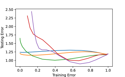
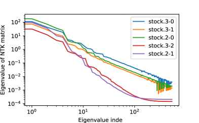
Figure 6: Left. Training/testing error trade-off on the “stock” dataset from the UCI regression dataset collection using kernel ridge regression with the neural tangent kernel. Each curve is labeled by “DatasetName.d-f” where “d” and “f” represents the number of layers and the number of fixed layers in the NTK corresponding to ReLU networks. Right. The eigenvalue index vs eigenvalue plot of the NTK matrix exhibits power-law spectra. A tiny value is added to the eigenvalues for better visualization on the log-scale.

References

- Arora et al., (2019) Arora, S., Du, S. S., Li, Z., Salakhutdinov, R., Wang, R., and Yu, D. (2019). Harnessing the power of infinitely wide deep nets on small-data tasks. In International Conference on Learning Representations.
- Arous and Guionnet, (2008) Arous, G. B. and Guionnet, A. (2008). The spectrum of heavy tailed random matrices. Communications in Mathematical Physics, 278(3):715–751.
- Bahri et al., (2021) Bahri, Y., Dyer, E., Kaplan, J., Lee, J., and Sharma, U. (2021). Explaining neural scaling laws. arXiv preprint arXiv:2102.06701.
- Bai and Silverstein, (2010) Bai, Z. and Silverstein, J. W. (2010). Spectral analysis of large dimensional random matrices, volume 20. Springer.
- Bartlett et al., (2020) Bartlett, P. L., Long, P. M., Lugosi, G., and Tsigler, A. (2020). Benign overfitting in linear regression. Proceedings of the National Academy of Sciences, 117(48):30063–30070.
- Belkin et al., (2018) Belkin, M., Ma, S., and Mandal, S. (2018). To understand deep learning we need to understand kernel learning. In International Conference on Machine Learning, pages 541–549. PMLR.
- Berthier et al., (2020) Berthier, R., Bach, F., and Gaillard, P. (2020). Tight nonparametric convergence rates for stochastic gradient descent under the noiseless linear model. Advances in Neural Information Processing Systems, 33:2576–2586.
- Bietti et al., (2021) Bietti, A., Venturi, L., and Bruna, J. (2021). On the sample complexity of learning with geometric stability. In Advances in Neural Information Processing Systems.
- Bordelon et al., (2020) Bordelon, B., Canatar, A., and Pehlevan, C. (2020). Spectrum dependent learning curves in kernel regression and wide neural networks. In International Conference on Machine Learning, pages 1024–1034. PMLR.
- Bubeck and Sellke, (2021) Bubeck, S. and Sellke, M. (2021). A universal law of robustness via isoperimetry. Advances in Neural Information Processing Systems, 34:28811–28822.
- Canatar et al., (2021) Canatar, A., Bordelon, B., and Pehlevan, C. (2021). Spectral bias and task-model alignment explain generalization in kernel regression and infinitely wide neural networks. Nature communications, 12(1):1–12.
- Cheng and Montanari, (2022) Cheng, C. and Montanari, A. (2022). Dimension free ridge regression. arXiv preprint arXiv:2210.08571.
- Couillet and Debbah, (2012) Couillet, R. and Debbah, M. (2012). Signal processing in large systems: A new paradigm. IEEE Signal Processing Magazine, 30(1):24–39.
- Cui et al., (2021) Cui, H., Loureiro, B., Krzakala, F., and Zdeborová, L. (2021). Generalization error rates in kernel regression: The crossover from the noiseless to noisy regime. In Advances in Neural Information Processing Systems, pages 10131–10143.
- Derezinski et al., (2019) Derezinski, M., Liang, F. T., and Mahoney, M. W. (2019). Exact expressions for double descent and implicit regularization via surrogate random design. ArXiv, abs/1912.04533.
- Dobriban and Wager, (2018) Dobriban, E. and Wager, S. (2018). High-dimensional asymptotics of prediction: Ridge regression and classification. The Annals of Statistics, 46(1):247–279.
- Dutka, (1984) Dutka, J. (1984). The early history of the hypergeometric function. Archive for History of Exact Sciences, pages 15–34.
- Ghosh and Belkin, (2022) Ghosh, N. and Belkin, M. (2022). A universal trade-off between the model size, test loss, and training loss of linear predictors. arXiv preprint arXiv:2207.11621.
- Goel and Klivans, (2017) Goel, S. and Klivans, A. (2017). Eigenvalue decay implies polynomial-time learnability for neural networks. Advances in Neural Information Processing Systems, 30.
- Hastie et al., (2022) Hastie, T., Montanari, A., Rosset, S., and Tibshirani, R. J. (2022). Surprises in High-Dimensional Ridgeless Least Squares Interpolation. The Annals of Statistics.
- (21) Jacot, A., Simsek, B., Spadaro, F., Hongler, C., and Gabriel, F. (2020a). Implicit regularization of random feature models. In International Conference on Machine Learning, pages 4631–4640. PMLR.
- (22) Jacot, A., Simsek, B., Spadaro, F., Hongler, C., and Gabriel, F. (2020b). Kernel alignment risk estimator: Risk prediction from training data. Advances in Neural Information Processing Systems, 33:15568–15578.
- Ji et al., (2021) Ji, Z., Li, J., and Telgarsky, M. (2021). Early-stopped neural networks are consistent. Advances in Neural Information Processing Systems, 34:1805–1817.
- Karp and López, (2017) Karp, D. B. and López, J. L. (2017). Representations of hypergeometric functions for arbitrary parameter values and their use. Journal of Approximation Theory, 218:42–70.
- Kausik et al., (2023) Kausik, C., Srivastava, K., and Sonthalia, R. (2023). Generalization error without independence: Denoising, linear regression, and transfer learning. arXiv preprint arXiv:2305.17297.
- Kelly et al., (2023) Kelly, M., Longjohn, R., and Nottingham, K. (2023). The uci machine learning repository. https://archive.ics.uci.edu.
- Knowles and Yin, (2017) Knowles, A. and Yin, J. (2017). Anisotropic local laws for random matrices. Probability Theory and Related Fields, 169(1):257–352.
- Koehler et al., (2021) Koehler, F., Zhou, L., Sutherland, D. J., and Srebro, N. (2021). Uniform convergence of interpolators: Gaussian width, norm bounds and benign overfitting. Advances in Neural Information Processing Systems, 34:20657–20668.
- Kuzborskij and Szepesvári, (2022) Kuzborskij, I. and Szepesvári, C. (2022). Learning lipschitz functions by gd-trained shallow overparameterized relu neural networks. arXiv preprint arXiv:2212.13848.
- Liang and Rakhlin, (2020) Liang, T. and Rakhlin, A. (2020). Just interpolate: Kernel “ridgeless” regression can generalize. The Annals of Statistics, 48(3):1329–1347.
- Mahoney and Martin, (2019) Mahoney, M. and Martin, C. (2019). Traditional and heavy tailed self regularization in neural network models. In International Conference on Machine Learning, pages 4284–4293. PMLR.
- Mallinar et al., (2022) Mallinar, N. R., Simon, J. B., Abedsoltan, A., Pandit, P., Belkin, M., and Nakkiran, P. (2022). Benign, tempered, or catastrophic: Toward a refined taxonomy of overfitting. In Advances in Neural Information Processing Systems.
- Murray et al., (2022) Murray, M., Jin, H., Bowman, B., and Montufar, G. (2022). Characterizing the spectrum of the NTK via a power series expansion. arXiv preprint arXiv:2211.07844.
- Nakkiran et al., (2020) Nakkiran, P., Venkat, P., Kakade, S. M., and Ma, T. (2020). Optimal regularization can mitigate double descent. In International Conference on Learning Representations.
- Paquette et al., (2021) Paquette, C., Lee, K., Pedregosa, F., and Paquette, E. (2021). Sgd in the large: Average-case analysis, asymptotics, and stepsize criticality. In Conference on Learning Theory, pages 3548–3626. PMLR.
- Paquette et al., (2022) Paquette, C., van Merriënboer, B., Paquette, E., and Pedregosa, F. (2022). Halting time is predictable for large models: A universality property and average-case analysis. Foundations of Computational Mathematics, pages 1–77.
- Silverstein and Choi, (1995) Silverstein, J. W. and Choi, S.-I. (1995). Analysis of the limiting spectral distribution of large dimensional random matrices. Journal of Multivariate Analysis, 54(2):295–309.
- Simon et al., (2023) Simon, J. B., Dickens, M., Karkada, D., and Deweese, M. (2023). The eigenlearning framework: A conservation law perspective on kernel ridge regression and wide neural networks. Transactions on Machine Learning Research.
- Sonthalia et al., (2023) Sonthalia, R., Li, X., and Gu, B. (2023). Under-parameterized double descent for ridge regularized least squares denoising of data on a line. arXiv preprint arXiv:2305.14689.
- Sonthalia and Nadakuditi, (2023) Sonthalia, R. and Nadakuditi, R. R. (2023). Training data size induced double descent for denoising feedforward neural networks and the role of training noise. Transactions on Machine Learning Research.
- Tao, (2011) Tao, T. (2011). Intuitive understanding of the Stieltjes transform. MathOverflow. Version: 2011-10-25.
- Tsigler and Bartlett, (2020) Tsigler, A. and Bartlett, P. L. (2020). Benign overfitting in ridge regression. arXiv preprint arXiv:2009.14286.
- Velikanov and Yarotsky, (2021) Velikanov, M. and Yarotsky, D. (2021). Explicit loss asymptotics in the gradient descent training of neural networks. Advances in Neural Information Processing Systems, 34:2570–2582.
- Velikanov and Yarotsky, (2022) Velikanov, M. and Yarotsky, D. (2022). Tight convergence rate bounds for optimization under power law spectral conditions. arXiv preprint arXiv:2202.00992.
- Wang et al., (2024) Wang, Z., Engel, A., Sarwate, A. D., Dumitriu, I., and Chiang, T. (2024). Spectral evolution and invariance in linear-width neural networks. Advances in Neural Information Processing Systems, 36.
- Wei et al., (2022) Wei, A., Hu, W., and Steinhardt, J. (2022). More than a toy: Random matrix models predict how real-world neural representations generalize. In Proceedings of the 39th International Conference on Machine Learning, pages 23549–23588. PMLR.
- Wu and Xu, (2020) Wu, D. and Xu, J. (2020). On the optimal weighted regularization in overparameterized linear regression. Advances in Neural Information Processing Systems, 33:10112–10123.
- Zhang et al., (2017) Zhang, C., Bengio, S., Hardt, M., Recht, B., and Vinyals, O. (2017). Understanding deep learning requires rethinking generalization. In International Conference on Learning Representations.
- Zhang et al., (2021) Zhang, C., Bengio, S., Hardt, M., Recht, B., and Vinyals, O. (2021). Understanding deep learning (still) requires rethinking generalization. Communications of the ACM, 64(3):107–115.
- Zhang et al., (2022) Zhang, H., Wu, Y., and Huang, H. (2022). How many data are needed for robust learning? arXiv preprint arXiv:2202.11592.