Advantage-Aware Policy Optimization for Offline Reinforcement Learning

Abstract

Offline Reinforcement Learning (RL) endeavors to leverage offline datasets to craft effective agent policy without online interaction, which imposes proper conservative constraints with the support of behavior policies to tackle the Out-Of-Distribution (OOD) problem. However, existing works often suffer from the constraint conflict issue when offline datasets are collected from multiple behavior policies, i.e., different behavior policies may exhibit inconsistent actions with distinct returns across the state space. To remedy this issue, recent Advantage-Weighted (AW) methods prioritize samples with high advantage values for agent training while inevitably leading to overfitting on these samples. In this paper, we introduce a novel Advantage-Aware Policy Optimization (A2PO) method to explicitly construct advantage-aware policy constraints for offline learning under mixed-quality datasets. Specifically, A2PO employs a Conditional Variational Auto-Encoder (CVAE) to disentangle the action distributions of intertwined behavior policies by modeling the advantage values of all training data as conditional variables. Then the agent can follow such disentangled action distribution constraints to optimize the advantage-aware policy towards high advantage values. Extensive experiments conducted on both the single-quality and mixed-quality datasets of the D4RL benchmark demonstrate that A2PO yields results superior to state-of-the-art counterparts. Our code will be made publicly available.

1 Introduction

Offline Reinforcement Learning (RL) (Fujimoto et al., 2019; Chen et al., 2020) aims to learn effective control policies from pre-collected datasets without online exploration, and has witnessed its unprecedented success in various real-world applications, including robot manipulation (Xiao et al., 2022; Wagenmaker & Pacchiano, 2023), recommendation system (Gao et al., 2023a; Sakhi et al., 2023), etc. A formidable challenge of offline RL lies in the Out-Of-Distribution (OOD) problem (Levine et al., 2020), involving the distribution shift between data induced by the learned policy and data collected by the behavior policy. Consequently, the direct application of conventional online RL methods inevitably exhibits extrapolation error (Prudencio et al., 2023), where the unseen state-action pairs are erroneously estimated. To tackle this OOD problem, offline RL methods attempt to impose proper conservatism on the learning agent within the distribution of the dataset, such as restricting the learned policy with a regularization term (Kumar et al., 2019; Fujimoto & Gu, 2021) or penalizing the value overestimation of OOD actions (Kumar et al., 2020; Kostrikov et al., 2021).

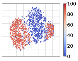
(a) Actual Return  

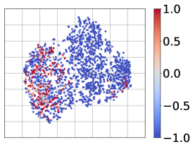
(b) LAPO Advantage Estimation 

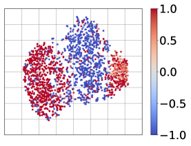
(c) A2PO Advantage Estimation 

Figure 1: Comparison of our proposed A2PO method and the state-of-the-art AW method (LAPO) in advantage estimation for the mixed-quality offline dataset (halfcheetah-random-expert-v2). Each data point represents an initial state-action pair in the offline dataset after applying PCA, while varying shades of color indicate the magnitude of the actual return or advantage value.

Despite the promising results achieved, offline RL often encounters the constraint conflict issue when dealing with the mixed-quality dataset (Chen et al., 2022; Singh et al., 2022; Gao et al., 2023b; Chebotar et al., 2023). Specifically, when training data are collected from multiple behavior policies with distinct returns, existing works still treat each sample constraint equally with no regard for the differences in data quality. This oversight can lead to conflict value estimation and further suboptimal results. To resolve this concern, the Advantage-Weighted (AW) methods employ weighted sampling to prioritize training transitions with high advantage values from the offline dataset (Chen et al., 2022; Tian et al., 2023; Zhuang et al., 2023). However, we argue that these AW methods implicitly reduce the diverse behavior policies associated with the offline dataset into a narrow one from the viewpoint of the dataset redistribution. As a result, this redistribution operation of AW may exclude a substantial number of crucial transitions during training, thus impeding the advantage estimation for the effective state-action space. To exemplify the advantage estimation problem in AW, we conduct a didactic experiment on the state-of-the-art AW method, LAPO (Chen et al., 2022), as shown in Figure 1. The results demonstrate that LAPO only accurately estimates the advantage value for a small subset of the high-return state-action pairs (left part of Figure 1b), while consistently underestimating the advantage value of numerous effective state-action pairs (right part of Figure 1b). These errors in advantage estimation can further lead to unreliable policy optimization.

In this paper, we propose Advantage-Aware Policy Optimization, abbreviated as A2PO, to explicitly learn the advantage-aware policy with disentangled behavior policies from the mixed-quality offline dataset. Unlike previous AW methods devoted to dataset redistribution while overfitting on high-advantage data, the proposed A2PO directly conditions the agent policy on the advantage values of all training data without any prior preference. Technically, A2PO comprises two alternating stages, behavior policy disentangling and agent policy optimization. The former stage introduces a Conditional Variational Auto-Encoder (CVAE) (Sohn et al., 2015) to disentangle different behavior policies into separate action distributions by modeling the advantage values of collected state-action pairs as conditioned variables. The latter stage further imposes an explicit advantage-aware policy constraint on the training agent within the support of disentangled action distributions. Combining policy evaluation and improvement with such advantage-aware constraint, A2PO can perform a more effective advantage estimation, as illustrated in Figure 1c, to further optimize the agent toward high advantage values to obtain the effective decision-making policy.

To sum up, our main contribution is the first dedicated attempt towards advantage-aware policy optimization to alleviate the constraint conflict issue under the mixed-quality offline dataset. The proposed A2PO can achieve advantage-aware policy constraint derived from different behavior policies, where a customized CVAE is employed to infer diverse action distributions associated with the behavior policies by modeling advantage values as conditional variables. Extensive experiments conducted on the D4RL benchmark (Fu et al., 2020), including both single-quality and mixed-quality datasets, demonstrate that the proposed A2PO method yields significantly superior performance to the state-of-the-art offline RL baselines, as well as the advantage-weighted competitors.

2 Related Works

Offline RL can be broadly classified into four categories: policy constraint (Fujimoto et al., 2019; Vuong et al., 2022), value regularization (Ghasemipour et al., 2022; Hong et al., 2022), model-based method (Zheng et al., 2023; Yang et al., 2023), and return-conditioned supervised learning (Emmons et al., 2021; Liu & Abbeel, 2023). Policy constraint methods impose constraints on the learned policy to be close to the behavior policy (Kumar et al., 2019). Previous studies directly introduce the explicit constraint on policy learning, such as behavior cloning (Fujimoto & Gu, 2021), maximum mean discrepancy (Kumar et al., 2019), or maximum likelihood estimation (Wu et al., 2022). In contrast, recent efforts (Nair et al., 2020; Wang et al., 2023) mainly focus on realizing the policy constraints implicitly by approximating the formal optimal policy derived from KL-divergence constraint. On the other hand, value regularization methods make constraints on the value function to alleviate the overestimation of OOD action. Researchers try to approximate the lower bound of the value function with the Q-regularization term for conservative action selection (Kumar et al., 2020; Lyu et al., 2022). Model-based methods construct the environment dynamics to estimate state-action uncertainty for OOD penalty (Karabag & Topcu, 2023; Diehl et al., 2023). Several works also converts offline RL into a return-conditioned supervised learning task. Decision Transformer (DT) (Chen et al., 2021) builds a transformer policy conditioned on both the current state and the additional sum return signal with supervised learning. Yamagata et al. (2023) improve the stitching ability of DT policy on sub-optimal samples by relabeling the return signal with Q-learning results. However, in the context of offline RL with a mixed-quality dataset and no access to the trajectory return signals, all these methods treat each sample equally without considering data quality, thereby resulting in conflict value estimation and further suboptimal learning outcomes.

Advantage-weighted Offline RL Method employs weighted sampling to prioritize training transitions with high advantage values from the offline dataset. To enhance sample efficiency, Peng et al. (2019) introduce an advantage-weighted maximum likelihood loss by directly calculating advantage values via trajectory return. (Nair et al., 2020) further use the critic network to estimate advantage values for advantage-weighted policy training. This technique has been incorporated as a subroutine in other works (Kostrikov et al., 2021; Xu et al., 2023) for agent policy extraction. Recently, AW methods have also been well studied in addressing the constraint conflict issue that arises from the mixed-quality dataset (Chen et al., 2022; Zhuang et al., 2023; Singh et al., 2022). Several studies present advantage-weighted behavior cloning as a direct objective function (Zhuang et al., 2023) or an explicit policy constraint (Peng et al., 2023). (Chen et al., 2022) propose the Latent Advantage-Weighted Policy Optimization (LAPO) framework, which employs an advantage-weighted loss to train CVAE for generating high-advantage actions based on the state condition. However, this AW mechanism inevitably suffers from overfitting to specific high-advantage samples. In contrast, our A2PO directly conditions the agent policy on both the state and the estimated advantage value, enabling effective utilization of all samples with varying quality.

3 Preliminaries

We formalize the RL task as a Markov Decision Process (MDP) (Puterman, 2014) defined by a tuple $\mathcal{M}=\langle\mathcal{S},\mathcal{A},P,r,\gamma,\rho_{0}\rangle$, where $\mathcal{S}$ represents the state space, $\mathcal{A}$ represents the action space, $P:\mathcal{S}\times\mathcal{A}\times\mathcal{S}\rightarrow\left[0,1\right]$ denotes the environment dynamics, $r:\mathcal{S}\times\mathcal{A}\rightarrow\mathbb{R}$ denotes the reward function, $\gamma\in(0,1]$ is the discount factor, and $\rho_{0}$ is the initial state distribution. At each time step $t$, the agent observes the state $s_{t}\in\mathcal{S}$ and selects an action $a_{t}\in\mathcal{A}$ according to its policy $\pi$. This action leads to a transition to the next state $s_{t+1}$ based on the dynamics distribution $P$. Additionally, the agent receives a reward signal $r_{t}$. The goal of RL is to learn an optimal policy $\pi^{*}$ that maximizes the expected return: $\pi^{*}=\arg\max_{\pi}\mathbb{E}_{\pi}\left[\sum_{k=0}^{\infty}\gamma^{k}r_{t+k}\right]$. In offline RL, the agent can only learn from an offline dataset without online interaction with the environment. In the single-quality settings, the offline dataset $\mathcal{D}=\left\{\left(s_{t},a_{t},r_{t},s_{t+1}\right)\mid t=1,\cdots,N\right\}$ with $N$ transitions is collected by only one behavior policy $\pi_{\beta}$. In the mixed-quality settings, the offline dataset $\mathcal{D}=\bigcup_{i}\left\{\left(s_{i,t},a_{i,t},r_{i,t},s_{i,t+1}\right)\mid t=1,\cdots,N\right\}$ is collected by multiple behavior policies $\{\pi_{{\beta}_{i}}\}_{i=1}^{M}$.

We evaluate the learned policy $\pi$ by the action value function $Q^{\pi}(s,a)=\mathbb{E}_{\pi}\left[\sum_{t=0}^{\infty}\gamma^{t}r(s_{t},a_{t})\mid s_{0}=s,a_{0}=a\right]$. The state value function is defined as $V^{\pi}(s)=\mathbb{E}_{a\sim\pi}\left[Q^{\pi}(s,a)\right]$, while the advantage function is defined as $A^{\pi}(s,a)=Q^{\pi}(s,a)-V^{\pi}(s)$. For continuous control, our A2PO implementation uses the TD3 algorithm (Fujimoto et al., 2018) based on the actor-critic framework as a basic backbone for its robust performance. The actor network $\pi_{\omega}$, known as the learned policy, is parameterized by $\omega$, while the critic networks consist of the Q-network $Q_{\theta}$ parameterized by $\theta$ and the V-network $V_{\phi}$ parameterized by $\phi$. The actor-critic framework involves two steps: policy evaluation and policy improvement. During policy evaluation phase, the Q-network $Q_{\theta}$ is optimized by following temporal-difference (TD) loss (Sutton & Barto, 2018):

$$\mathcal{L}_{Q}(\theta)=\mathbb{E}_{(s,a,r,s^{\prime})\sim\mathcal{D},a^{\prime}\sim\pi_{\hat{\omega}}(s^{\prime})}\bigl{[}Q_{\theta}(s,a)-\\ \left(r(s,a)+\gamma Q_{\hat{\theta}}(s^{\prime},a^{\prime})\right)\bigr{]}^{2},$$ (1)

where $\hat{\theta}$ and $\hat{\omega}$ are the parameters of the target networks that are regularly updated by online parameters $\theta$ and ${\omega}$ to maintain learning stability. The V-network $V_{\phi}$ can also be optimized by the similar TD loss. For policy improvement in continuous control, the actor network $\pi_{\omega}$ can be optimized by the deterministic policy gradient loss (Silver et al., 2014; Schulman et al., 2017):

$$\mathcal{L}_{\pi}(\omega)=\mathbb{E}_{s\sim\mathcal{D}}\left[-Q_{\theta}(s,\pi_{\omega}(s))\right].$$ (2)

Note that offline RL will impose conservative constraints on the optimization losses to tackle the OOD problem. Moreover, the performance of the final learned policy $\pi_{\omega}$ highly depends on the quality of the offline dataset $\mathcal{D}$ associated with the behavior policies $\{\pi_{{\beta}_{i}}\}$.

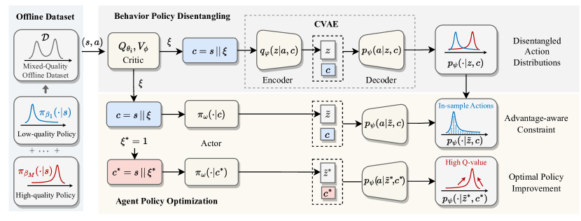
Figure 2: An illustrative diagram of the Advantage-Aware Policy Optimization (A2PO) method.

4 Methodology

In this section, we provide details of our proposed A2PO approach, consisting of two key components: behavior policy disentangling and agent policy optimization. In the behavior policy disentangling phase, we disentangle behavior policies with a CVAE specifically modeling the action distribution conditioned on the advantage values of collected state-action pairs. By taking different advantage inputs, the newly formed CVAE allows the agent to infer distinct action distributions that are associated with various behavior policies. Then in the agent policy optimization phase, the action distributions derived from the advantage condition serve as disentangled behavior policies, establishing an advantage-aware policy constraint to guide agent training. An overview of our A2PO is illustrated in Figure 2.

4.1 Behavior Policy Disentangling

To realize behavior policy disentangling, we adopt a CVAE to relate the behavior distribution of different specific behavior policies $\pi_{\beta_{i}}$ to the advantage-based condition variables, which is quite different from previous methods (Fujimoto et al., 2019; Chen et al., 2022; Zhou et al., 2021) utilizing CVAE only for approximating the overall mixed-quality behavior policy set $\left\{\pi_{\beta_{i}}\right\}_{i=1}^{M}$ conditioned only on specific state $s$. Concretely, we have made adjustments to the architecture of the CVAE to be advantage-aware. The encoder $q_{\varphi}(z|a,c)$ is fed with condition $c$ and action $a$ to project them into a latent representation $z$. Given specific condition $c$ and the encoder output $z$, the decoder $p_{\psi}(a|z,c)$ captures the correlation between condition $c$ and latent representation $z$ to reconstruct the original action $a$. Unlike previous methods (Fujimoto et al., 2019; Chen et al., 2022; Wu et al., 2022) predicting action solely based on the state $s$, we consider both state $s$ and advantage value $\xi$ for CVAE condition. The state-advantage condition $c$ is formulated as:

$$c=s\,||\,\xi.$$ (3)

Therefore, given the current state $s$ and the advantage value $\xi$ as a joint condition, the CVAE model is able to generate corresponding action $a$ with varying quality positively correlated with the advantage value $\xi$. For a state-action pair $(s,a)$, the advantage value $\xi$ can be computed as follows:

$$\xi=\tanh\big{(}\min_{i=1,2}Q_{\theta_{i}}(s,a)-V_{\phi}(s)\big{)},$$ (4)

where two Q-networks with the $\min(\cdot)$ operation are adopted to ensure conservatism in offline RL settings (Fujimoto et al., 2019). Moreover, we employ the $\tanh(\cdot)$ function to normalize the advantage condition within the range of $(-1,1)$. This operation prevents excessive outliers from impacting the performance of CVAE, improving the controllability of generation. The optimization of Q-networks and V-network will be described in the following section.

The CVAE model is trained using the state-advantage condition $c$ and the corresponding action $a$. The training objective involves maximizing the Empirical Lower Bound (ELBO) (Sohn et al., 2015) on the log-likelihood of the sampled minibatch:

$$\mathcal{L}_{\text{CVAE}}({\varphi,\psi})=-\mathbb{E}_{\mathcal{D}}\bigl{[}\mathbb{E}_{q_{\varphi}(z|a,c)}\left[\log(p_{\psi}(a|z,c))\right]\\ +\alpha\cdot\text{KL}\left[q_{\varphi}(z|a,c)\parallel p(z)\right]\bigr{]},$$ (5)

where $\alpha$ is the coefficient for trading off the KL-divergence loss term, and $p(z)$ denotes the prior distribution of $z$ setting to be $\mathcal{N}(0,1)$. The first log-likelihood term encourages the generated action to match the real action as much as possible, while the second KL divergence term aligns the latent variable distribution with the prior distribution $p(z)$.

At each round of CVAE training, a minibatch of state-action pairs $(s,a)$ is sampled from the offline dataset. These pairs are fed to the critic network $Q_{\theta}$ and $V_{\phi}$ to get corresponding advantage condition $\xi$ by Equation (4). Then the advantage-aware CVAE is subsequently optimized by Equation (5). By incorporating the advantage condition $\xi$ into the CVAE, the CVAE captures the relation between $\xi$ and the action distribution of the behavior policies, as shown in the upper part of Figure 2. This further enables the CVAE to generate actions $a$ based on the state-advantage condition $c$ in a manner where the action quality is positively correlated with $\xi$. Furthermore, the advantage-aware CVAE is utilized to establish an advantage-aware policy constraint for agent policy optimization in the next stage.

4.2 Agent Policy Optimization

The agent is constructed using the actor-critic framework (Sutton & Barto, 2018). The critic comprises two Q-networks $Q_{\theta_{i=1,2}}$ and one V-network $V_{\phi}$ to approximate the value of the agent policy. The actor, advantage-aware policy $\pi_{\omega}(\cdot|c)$, with input $c=s\,||\,\xi$, generates a latent representation $\tilde{z}$ based on the state $s$ and the designated advantage condition $\xi$. This latent representation $\tilde{z}$, along with $c$, is then fed into the decoder $p_{\psi}$ for an recognizable action $a_{\xi}$:

$$a_{\xi}\sim p_{\psi}(\cdot\mid\tilde{z},c),\;\text{where}\;\tilde{z}\sim\pi_{\omega}(\cdot\mid c).$$ (6)

With this form, the advantage-aware policy $\pi_{\omega}$ is expected to produce action with different qualities that are positively correlated to the designated advantage input $\xi$ which is normalized within $(-1,1)$ in Equation (4). Therefore, the output optimal action $a^{*}$ is obtained by $c^{*}=s\,||\,\xi^{*}$ input with $\xi^{*}=1$. It should be noted that the critic networks are to approximate the expected value of the optimal policy $\pi_{\omega}(\cdot|c^{*})$. The agent optimization, following the actor-critic framework, encompasses policy evaluation and policy improvement steps. During the policy evaluation step, the critic is optimized through the minimization of the temporal difference loss with the optimal policy $\pi_{\omega}(\cdot|c^{*})$, as follows:

$$\mathcal{L}_{\text{TD}}(\theta,\phi)=\mathbb{E}_{\begin{subarray}{c}(s,a,r,s^{\prime})\sim\mathcal{D},\\ \tilde{z}^{*}\sim\pi_{\omega}(\cdot|c^{*}),\\ a^{*}_{\xi}\sim p_{\psi}(\cdot|\tilde{z}^{*},c^{*})\end{subarray}}\Big{[}\scalebox{0.95}[1.0]{$\sum$}_{i}\big{[}r+V_{\hat{\phi}}(s)-Q_{\theta_{i}}(s,a)\big{]}^{2}\\ +\big{[}r+\min_{i}Q_{\hat{\theta}_{i}}(s^{\prime},a^{*}_{\xi})-V_{\phi}(s)\big{]}^{2}\Big{]},$$ (7)

where $Q_{\hat{\theta}}$ and $V_{\hat{\phi}}$ are the target networks updated softly. The first term of $\mathcal{L}_{\text{TD}}$ is to optimize the Q-network while the second term is for the V-network. Different from Equation (1), we introduce the target Q and V simultaneously to stablily optimize the mutual online network.

For the policy improvement, the actor loss is defined as:

$$\mathcal{L}_{\text{AC}}(\omega)=-\lambda\cdot\mathbb{E}_{\begin{subarray}{c}s\sim\mathcal{D},\tilde{z}^{*}\sim\pi_{\omega}(\cdot|c^{*}),\\ a^{*}_{\xi}\sim p_{\psi}(\cdot|\tilde{z}^{*},c^{*})\end{subarray}}\big{[}Q_{\theta_{1}}(s,a^{*}_{\xi})\big{]}\\ +\mathbb{E}_{\begin{subarray}{c}(s,a)\sim\mathcal{D},\tilde{z}\sim\pi_{\omega}(\cdot|c),\\ a_{\xi}\sim p_{\psi}(\cdot|\tilde{z},c)\end{subarray}}\big{[}(a-a_{\xi})^{2}\big{]},$$ (8)

where $a^{*}_{\xi}$ in the first term is the optimal action generated with the fixed maximum advantage condition $\xi^{*}=1$ input and $a_{\xi}$ in the second term is obtained with the advantage condition $\xi$ derived from the critic based on Equation (4) applied to the sampled batch. Meanwhile, following TD3+BC (Fujimoto & Gu, 2021), we add a normalization coefficient $\lambda={\alpha}/{\big{(}\frac{1}{N}\sum_{(s_{i},a_{i})}|Q(s_{i},a_{i})|\big{)}}$ to the first term to keep the scale balance between Q value objective and regularization, where $\alpha$ is a hyperparameter to control the scale of the normalized Q value. The first term encourages the optimal policy condition on $c^{*}$ to select actions that yield the highest expected returns represented by the Q-value. This aligns with the policy improvement step in conventional reinforcement learning approaches. The second behavior cloning term explicitly imposes constraints on the advantage-aware policy, ensuring the policy selects in-sample actions that adhere to the advantage condition $\xi$ determined by the critic. Therefore, the suboptimal samples with low advantage condition $\xi$ will not disrupt the optimization of optimal policy $\pi_{\omega}(\cdot|c^{*})$. And they enforce valid constraints on the corresponding policy $\pi_{\omega}(\cdot|c)$, as shown in the lower part of Figure 2. It should be noted that the decoder $p_{\psi}$ is fixed during both policy evaluation and improvement.

Our A2PO implementation selects TD3+BC (Fujimoto & Gu, 2021) as the base backbone for its robustness and conciseness. The general framework derived above is thoroughly described in Appendix A.

5 Experiments

To illustrate the effectiveness of the proposed A2PO method, we conduct experiments on the D4RL benchmark (Fu et al., 2020). We aim to answer the following questions: (1) Can A2PO outperform the state-of-the-art offline RL methods in both the single-quality datasets and mixed-quality datasets? (Section 5.2) (2) How do different components of A2PO contribute to the overall performance? (Section 5.3 and Appendix C–G) (3) How does A2PO perform under mixed-quality datasets with varying single-quality samples? (Section 5.4 and Appendix H) (4) Can the A2PO agent effectively estimate the advantage value of different transitions? (Section 5.5 and Appendix I)

5.1 Experiment Settings

Tasks and Datasets. We consider four different domains of tasks in D4RL benchmark (Fu et al., 2020): Gym, Maze, Adroit, and Kitchen. Each domain contains several tasks and corresponding distinct datasets. We conduct experiments for each Gym task using single-quality and mixed-quality datasets. The single-quality datasets are generated with the medium behavior policy. The mixed-quality datasets are combinations of random, medium, and expert single-quality datasets, including medium-expert, medium-replay, random-medium, medium-expert, and random-medium-expert. The D4RL benchmark only includes the first two mixed-quality datasets. Thus, following Hong et al. (2023b, a), we manually construct the last three mixed-quality datasets by directly combining the corresponding single-quality datasets in D4RL with equal proportions. For the other domains of tasks, the corresponding D4RL datasets exhibit a significant level of diversity, which enables us to evaluate the effectiveness of our A2PO algorithm.

Table 1: Test returns of our proposed A2PO and baselines on the Gym tasks. $\pm$ corresponds to one standard deviation of the average evaluation of the performance on 5 random seeds. The performance is measured by the normalized scores at the last training iteration. Bold indicates the best performance in each task.

Source	Task	BC	BCQ	TD3+BC	CQL	MOPO	EQL	Diffusion-QL	AWAC	IQL	CQL+AW	LAPO	A2PO (Ours)
medium	halfcheetah	42.6	47.0	48.3	44.0	42.3	47.2	51.1	43.5	47.4	46.5	46.0	47.1 $\pm$	0.2
	hopper	52.9	56.7	59.3	58.5	28.0	74.6	70.3	57.0	66.3	67.7	51.6	80.3 $\pm$	4.0
	walker2d	75.3	72.6	83.7	72.5	17.8	83.2	83.5	72.4	78.3	81.3	80.8	84.9 $\pm$	0.2
medium replay	halfcheetah	36.6	40.4	44.6	45.5	53.1	44.5	46.3	40.5	44.2	44.7	41.9	44.8 $\pm$	0.2
	hopper	18.1	53.3	60.9	98.1	67.5	98.1	100.2	37.2	94.7	97.0	50.1	101.6 $\pm$	1.3
	walker2d	26.0	52.1	81.8	81.6	39.0	76.6	90.6	27.0	73.9	78.1	60.6	82.8 $\pm$	1.7
medium expert	halfcheetah	55.2	89.1	90.7	91.6	63.3	90.6	94.3	42.8	86.7	89.4	94.2	95.6 $\pm$	0.5
	hopper	52.5	81.8	98.0	105.4	23.7	105.5	111.1	55.8	91.5	104.6	111.0	113.4 $\pm$	0.5
	walker2d	107.5	109.0	110.1	108.8	44.6	110.2	110.1	74.5	109.6	109.3	110.9	112.1 $\pm$	0.2
random medium	halfcheetah	2.3	12.7	47.7	31.9	52.7	42.3	48.4	46.5	42.2	46.5	18.5	48.5 $\pm$	0.3
	hopper	23.2	9.2	7.4	3.3	19.9	1.7	6.9	19.5	6.2	22.6	4.2	62.1 $\pm$	2.8
	walker2d	19.2	0.2	10.7	0.2	40.2	31.4	3.3	0.0	54.6	82.0	23.6	82.3 $\pm$	0.4
random expert	halfcheetah	13.7	2.1	43.1	15.0	18.5	47.4	86.1	87.3	28.6	80.7	52.6	90.3 $\pm$	1.6
	hopper	10.1	8.5	78.8	7.8	17.2	68.6	102.0	84.7	58.5	109.6	82.3	112.5 $\pm$	1.3
	walker2d	14.7	0.6	7.0	0.3	4.6	9.1	56.3	11.7	90.9	108.6	0.4	109.1 $\pm$	1.4
random medium expert	halfcheetah	2.3	15.9	62.3	13.5	26.7	42.8	81.2	2.3	61.6	76.8	71.1	90.6 $\pm$	1.6
	hopper	27.4	4.0	60.5	9.4	13.3	72.4	70.1	8.6	57.9	71.8	66.6	107.8 $\pm$	0.4
	walker2d	24.6	2.4	15.7	0.1	56.4	61.0	56.6	-0.4	90.8	58.3	60.4	97.7 $\pm$	6.7
Gym Total		604.2	657.6	1010.6	787.5	628.8	1107.2	1268.4	710.9	1183.9	1303.7	1026.8	1583.7

Comparison Methods and Hyperparameters. We compare the proposed A2PO to several state-of-the-art offline RL methods: BCQ (Fujimoto et al., 2019), TD3+BC (Fujimoto & Gu, 2021), CQL (Kumar et al., 2020), EQL (Xu et al., 2023), especially the advantage-weighted offline RL methods: AWAC (Nair et al., 2020), IQL (Kostrikov et al., 2021), CQL+AW (Hong et al., 2023a), LAPO (Chen et al., 2022). Besides, we also select the vanilla BC method (Pomerleau, 1991), the model-based offline RL method MOPO (Yu et al., 2020), and the emerging diffusion-based method Diffusion-QL (Wang et al., 2022), for comparison. We report the performance of baselines using the best results reported from their own paper. The detailed hyperparameters of A2PO are given in Appendix B.2.

5.2 Comparison on D4RL Benchmarks

Results for Gym Tasks. The experimental results of all compared methods in the D4RL Gym tasks are presented in Table 1. For the single-quality medium dataset and mixed-quality medium-expert and medium-replay datasets from D4RL, our A2PO achieves state-of-the-art results with low variance. Meanwhile, both conventional offline RL approaches like EQL and advantage-weighted approaches like LAPO still learn acceptable policy, indicating that the conflict issue hardly occurs in these datasets with low diversity. However, the newly constructed mixed-quality datasets, namely random-medium, random-expert, and random-medium-expert, highlight the issue of substantial gaps between behavior policies. The results on these datasets reveal a significant drop in performance for all other baselines. Instead, our A2PO continues to achieve the best performance on these datasets. When considering the total scores across all datasets, A2PO outperforms the next best-performing AW method, CQL+AW, by over 21%. The results reveal the exceptional ability of A2PO to capture and utilize high-quality interactions within the dataset in order to enforce a reasonable advantage-aware policy constraint and further obtain an optimal agent policy.

Results for Maze, Kitchen, and Adroit Tasks. Table 2 presents the experimental results of all the compared methods on the D4RL Maze, Kitchen, and Adroit tasks. The D4RL datasets for these tasks exhibit varying patterns in behavior policy samples. For instance, the Antmaze datasets are highly sub-optimal, while the Adroit datasets have a narrow state-action distribution. Among the offline RL baselines and AW methods, A2PO delivers remarkable performance in these challenging tasks and showcases the robust representation capabilities of the advantage-aware policy.

Table 2: Test returns of our proposed A2PO and baselines on the Maze, Kitchen, and Adroit tasks.

Task	BC	BCQ	TD3+BC	CQL	MOPO	EQL	Diffusion-QL	AWAC	IQL	CQL+AW	LAPO	A2PO (Ours)
maze2d-umaze	0.5	24.8	24.2	5.7	-15.4	56.5	66.7	94.5	56.2	19.6	78.0	133.3 $\pm$	9.6
maze2d-medium	0.7	22.5	33.5	5.0	19.0	36.3	100.6	31.4	25.7	22.6	43.2	114.9 $\pm$	12.9
maze2d-large	1.1	43.0	128.5	12.5	-0.5	57.0	116.3	43.9	45.7	10.3	69.7	156.4 $\pm$	5.8
antmaze-umaze-diverse	45.6	55.0	71.4	84.0	0.0	65.4	24.0	49.3	62.2	36.0	84.1	93.3 $\pm$	4.7
antmaze-medium-diverse	0.0	0.0	3.0	53.7	0.0	70.0	46.4	0.7	70.0	6.0	1.2	86.7 $\pm$	9.4
antmaze-large-diverse	0.0	2.2	0.0	14.9	0.0	42.5	56.6	1.0	47.5	2.0	0.0	53.3 $\pm$	4.7
Maze Total	47.9	147.5	260.6	175.8	3.1	327.7	410.6	220.8	307.3	96.5	276.2	637.9
kitchen-complete	33.8	8.1	0.8	43.8	40.1	70.3	84.0	3.8	62.5	30.2	53.2	69.2 $\pm$	4.9
kitchen-partial	33.8	18.9	0.0	49.8	6.7	74.5	60.5	0.3	46.3	36.0	53.7	75.8 $\pm$	2.4
kitchen-mixed	47.5	10.6	0.8	51.0	17.3	55.6	62.6	0.0	51.0	50.5	62.4	64.2 $\pm$	3.1
Kitchen Total	115.1	37.6	1.6	144.6	64.1	200.4	207.1	4.1	159.8	116.7	169.3	209.2
pen-human	34.4	12.3	-3.7	37.5	54.6	44.3	72.8	4.3	71.5	-3.0	68.1	68.9 $\pm$	5.9
pen-cloned	56.9	28.0	1.7	39.2	10.7	46.9	57.3	-0.8	37.3	-2.5	55.8	85.0 $\pm$	7.3
Adroit Total	91.3	40.3	-2.0	76.7	65.3	91.2	130.1	3.5	108.8	-5.5	123.9	153.9

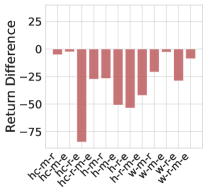
(a) $\xi_{\text{fix}}=1$

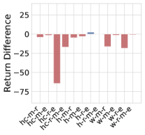
(b) $\xi_{\text{dis}}$ with $\epsilon=0.0$

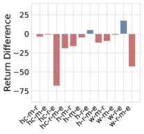
(c) $\xi_{\text{dis}}$ with $\epsilon=0.1$

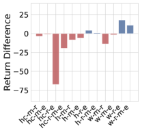
(d) $\xi_{\text{dis}}$ with $\epsilon=0.5$

Figure 3: Test return difference of A2PO with different discrete advantage conditions during training compared with original A2PO with continuous advantage condition during training. Task abbreviations are listed in Appendix B.1. Test returns are reported in Appendix C.

5.3 Ablation Analysis

Different Advantage condition during training. The performance comparison of different advantage condition computing methods for agent training is given in Figure 3. Equation (4) obtains continuous advantage condition $\xi$ in the range of $(-1,1)$. To evaluate the effectiveness of the continuous computing method, we design a discrete form of advantage condition: $\xi_{\text{dis}}=\text{sgn}(\xi)\cdot\mathbf{1}_{|\xi|>\epsilon}$, where $\text{sgn}(\cdot)$ is the symbolic function, and $\mathbf{1}_{|\xi|>\epsilon}$ is the indicator function returning $1$ if the absolute value of $\xi$ is greater than the hyperparameter of threshold $\epsilon$, otherwise $0$. Thus, the advantage condition $\xi_{\text{dis}}$ is constrained to discrete value of $\left\{-1,0,1\right\}$. Another special form of advantage condition is $\xi_{\text{fix}}=1$ for all state-action pairs, in which the advantage-aware ability is lost. Figure 3a shows that setting $\xi_{\text{fix}}=1$ without explicitly advantage-aware mechanism leads to a significant performance decreasing, especially in the new mixed-quality dataset. Meanwhile, $\xi_{\text{dis}}$ with different values of threshold $\epsilon$ achieve slightly inferior results than the continuous $\xi$. This outcome strongly supports the efficiency of continuous $\xi$. Although the $\xi_{\text{dis}}$ signals are more stable, $\xi_{\text{dis}}$ hidden the concrete advantage value, causing a mismatch between the advantage value and the sampled transition.

(a)

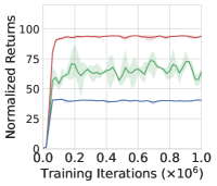
(a) halfcheetah
 (medium-expert)

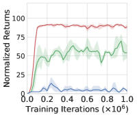
(b) halfcheetah
 (random-medium-expert)

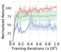
(c) hopper
 (medium-expert)

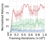
(d) hopper
 (random-medium-expert)

Figure 4: Learning curves of A2PO under different fixed advantage inputs during the test while using the original continuous advantage condition for training. Test returns are reported in Appendix D.

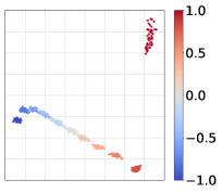
(a) walker2d-medium-replay
 (Advantage condition)

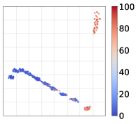
(b) walker2d-medium-replay
 (Actual Return)

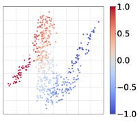
(c) hopper-medium-replay
 (Advantage condition)

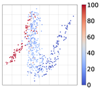
(d) hopper-medium-replay
 (Actual Return)

Figure 5: Visualization of A2PO latent representation after applying PCA with different advantage conditions and actual returns. Each data point indicates a latent representation $\tilde{z}$ based on the initial state and different advantage conditions sampled uniformly from $[-1,1]$. The actual return is measured under the corresponding sampled advantage condition. The value magnitude is indicated with varying shades of color.

Different Advantage Condition for Test. The performance comparison of different discrete advantage conditions input for the test is given in Figure 4. To ensure clear differentiation, we select $\xi$ from $\left\{-1,0,1\right\}$. The different designated advantage conditions $\xi$ are fixed input for the actor, leading to different policies $\pi_{\omega}(\cdot|s,\xi)$. The final outcomes demonstrate the partition of returns corresponding to the policies with different $\xi$. Furthermore, the magnitude of the gap increases as the offline dataset includes samples from more diverse behavior policies. These observations provide strong evidence for the success of A2PO disentangling the behavior policies under the multi-quality dataset.

(a)

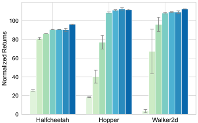
Figure 6: Compare the test returns of A2PO under random-expert dataset with different component proportions $\sigma$ in the Gym tasks. The datasets consist of $1\times 10^{6}$ samples, where $\sigma$ of the samples originate from the expert dataset and the remaining $1-\sigma$ of the samples come from the random dataset. Detail test returns are reported in Appendix H.

5.4 Robustness

Figure 6 presents the experimental results of A2PO across mixed-quality datasets with varying proportions of single-quality samples. Following the methodology of (Hong et al., 2023a, b), we assess the performance of A2PO on medium-expert, random-medium, and random-expert datasets while varying the proportions $\sigma$ of relatively higher quality samples while keeping proportions $1-\sigma$ for relatively lower quality samples. The results demonstrate that our A2PO effectively captures and infers high-quality potential behavior policies for proper policy regularization, even with a small proportion of high-quality samples. Additionally, as the $\sigma$ becomes larger, the variance decreases. Thus, A2PO demonstrates its robustness in handling variations in the proportions of different single-quality samples, guaranteeing consistently high performance.

5.5 Visualization

Figure 5 presents the visualization of A2PO latent representation. The uniformly sampled advantage condition $\xi$ combined with the initial state $s$, are fed into the actor-network to get the latent representation generated by the final layer of the actor. The result demonstrates that the representations converge according to the advantage and the actual return. Notably, the return of each point aligns with the corresponding variations in $\xi$. Moreover, as $\xi$ increases monotonically, the representations undergo continuous alterations in a rough direction. These observations suggest the effectiveness of advantage-aware policy construction. Meanwhile, more experiments of advantage estimation conducted on different tasks and datasets are presented in Appendix I.

6 Conclusion

In this paper, we propose a novel approach, termed as A2PO, to tackle the constraint conflict issue on mixed-quality offline datasets with advantage-aware policy constraints. Specifically, A2PO utilizes a CVAE to effectively disentangle the action distributions associated with various behavior policies. This is achieved by modeling the advantage values of all training data as conditional variables. Consequently, advantage-aware agent policy optimization can be focused on maximizing high advantage values while conforming to the disentangled distribution constraint imposed by the mixed-quality dataset. Experimental results show that A2PO successfully decouples the underlying behavior policies and significantly outperforms state-of-the-art offline RL competitors. For our future work, we will extend A2PO to multi-task offline RL scenarios characterized by a greater diversity of behavior policies and a more prominent constraint conflict issue.

Boarder Impact

This paper presents an offline advantage-aware learning approach that leverages the estimated advantage condition to deal with mixed-quality datasets. The advantage-aware concept brings a new perspective to the solution of real-world RL tasks, facilitating a more practical and effective utilization of the offline datasets. It has the potential to enhance the robustness of the agent towards the varying offline datasets from real-world RL scenarios, where the pre-collected offline datasets are noisy and often not as well-organized as the D4RL standardized datasets.

Appendix A Pseudocode

To make the proposed A2PO method clearer for readers, the pseudocode is provided in Algorithm 1.

Algorithm 1 Advantage-Aware Policy Optimization (A2PO)

Input: offline dataset $\mathcal{D}$, CVAE training step $K$, total training step $T$, soft update rate $\tau$.

Initialize: CVAE encoder $q_{\varphi}$ and decoder $p_{\psi}$, actor network $\pi_{\omega}$, critic networks $Q_{\theta}$ and $V_{\phi}$.

  for $i=1$ to $T$ do

     Sample random minibatch of transitions $\mathcal{B}=\{(s,a,r,s^{\prime})\}\sim\mathcal{D}$.

     Calculate $\xi=\tanh(\min_{i=1,2}Q_{\theta_{i}}(s,a)-V_{\phi}(s)),\xi^{*}=1,c=s||\xi,c^{*}=s||\xi^{*}$.

     # Behavior Policy Disentangling

     if $i\leq K$ then

        Optimize CVAE encoder $q_{\varphi}$ and decoder $p_{\psi}$ according to Equation (5) as

        

$$\mathcal{L}_{\text{CVAE}}({\varphi,\psi})=-\mathbb{E}_{\mathcal{D}}\left[\mathbb{E}_{q_{\varphi}(z|a,c)}\left[\log(p_{\psi}(a|z,c))\right]+\alpha\cdot\text{KL}\left[\left(q_{\varphi}(z|a,c)\parallel p(z)\right)\right]\right].$$

     end if

     # Agent Policy Optimization

     Optimize critic networks $Q_{\theta}$ and $V_{\phi}$ according to Equation (7) as

     

$$\mathcal{L}_{\text{TD}}(\theta,\phi)=\mathbb{E}_{\begin{subarray}{c}(s,a,r,s^{\prime})\sim\mathcal{D},\\ \tilde{z}^{*}\sim\pi_{\omega}(\cdot|c^{*}),\\ a^{*}_{\xi}\sim p_{\psi}(\cdot|\tilde{z}^{*},c^{*})\end{subarray}}\bigg{[}\sum_{i}\big{[}r+V_{\hat{\phi}}(s)-Q_{\theta_{i}}(s,a)\big{]}^{2}+\big{[}r+\min_{i}Q_{\hat{\theta}_{i}}(s^{\prime},a^{*}_{\xi})-V_{\phi}(s)\big{]}^{2}\bigg{]}.$$

     Optimize actor network $\pi_{\omega}$ according to Equation (8) as

     

$$\mathcal{L}_{\text{AC}}(\omega)=-\lambda\cdot\mathbb{E}_{\begin{subarray}{c}s\sim\mathcal{D},\\ \tilde{z}^{*}\sim\pi_{\omega}(\cdot|c^{*}),\\ a^{*}_{\xi}\sim p_{\psi}(\cdot|\tilde{z}^{*},c^{*})\end{subarray}}\big{[}Q_{\theta_{1}}(s,a^{*}_{\xi})\big{]}+\mathbb{E}_{\begin{subarray}{c}(s,a)\sim\mathcal{D},\\ \tilde{z}\sim\pi_{\omega}(\cdot|c),\\ a_{\xi}\sim p_{\psi}(\cdot|\tilde{z},c)\end{subarray}}\big{[}(a-a_{\xi})^{2}\big{]}.$$

     Update the target networks with $\hat{\theta}\leftarrow(1-\tau)\hat{\theta}+\tau\theta,\hat{\phi}\leftarrow(1-\tau)\hat{\phi}+\tau\phi$.

  end for

Appendix B Experiment Details

B.1 Task Abbreviations and Task Versions

In order to improve the readability and conciseness, we adopt abbreviations for the Gym tasks throughout the main text. The corresponding abbreviations for each task are provided in Table 3. For the specific task versions, we use the ‘-v2’ version for the Gym tasks, the ‘-v1’ version for the Maze2d tasks, the ‘-v2’ version for the Antmaze tasks, the ‘-v0’ version for the Kitchen tasks, the ‘-v1’ version for the Adroit tasks.

Table 3: The abbreviation of the corresponding Gym task and dataset.

Dataset	halfcheetah	hopper	walker2d
random	hc-r	h-r	w-r
medium	hc-m	h-m	w-m
expert	hc-e	h-e	w-e
medium-replay	hc-m-r	h-m-r	w-m-r
medium-expert	hc-m-e	h-m-e	w-m-e
random-medium	hc-r-m	h-r-m	w-r-m
random-expert	hc-m-e	h-m-e	w-m-e
random-medium-expert	hc-r-m-e	h-r-m-e	w-r-m-e

B.2 Implementation Details

In this section, we provide the implementation details of our experiments. We conducted our experiments using PyTorch 3.8 (Paszke et al., 2019) on a cluster of 8 A6000 GPUs. Each run required approximately 8 hours to complete 1 million steps. The source code will be made publicly available upon the publication of this paper.

The critic, actor, and CVAE networks are all constructed using a 2-layer MLP with 256 hidden units. They are updated using the Adam optimizer with a learning rate of $3\times 10^{-4}$. Additionally, we employ a target critic network with a soft-update rate of $5\times 10^{-3}$. Following the TD+3BC approach (Fujimoto & Gu, 2021), we incorporate Q normalization, policy noise, and policy clipping during the training process. For the hyperparameter value $\alpha$ in Q normalization, following the strategy of Wang et al. (2022), we set $\alpha=5.0$ for Antmaze tasks to emphasize strong and stable Q Learning. For other tasks, setting $\alpha=1.0$ produces state-of-the-art results. Among the tasks, the continuous form of the advantage signal $\xi$, as described in Equation (4), consistently yields excellent results. The only exception is the maze2d-umaze task, where utilizing a discrete form with $\epsilon=0.1$ achieves similarly high performance. Further details on the sensitivity of the $\xi$ type can be found in Section 5.3 and Appendix E. Furthermore, through practical experimentation, we have observed that the CVAE train step has an influence to the final performance. After performing a simple hyperparameter search, we found that the optimal settings are $4\times 10^{5}$ for maze2d-umaze and maze2d-medium tasks, and $2\times 10^{5}$ for the other tasks.

Since all of the original papers of other baselines do not provide the complete results of all the tasks, we make implementation of the baselines. The CQL, IQL and MOPO baselines are implemented using the implementations provided at github.com/young-geng/cql, gwthomas/iql-pytorch, and github.com/yihaosun1124/OfflineRL-Kit, respectively. The remaining baselines, including BCQ, CQL, TD3+BC, EQL, Diffusion-QL, AWAC, CQL+AW, and LAPO, are implemented using the original implementations provided by the authors of the respective papers. These implementations can be found at: BCQ github.com/sfujim/BCQ, TD3+BC github.com/sfujim/TD3_BC, EQL github.com/ryanxhr/IVR, Diffusion-QL github.com/Zhendong-Wang/Diffusion-Policies-for-Offline-RL, AWAC github.com/rail-berkeley/rlkit/tree/master/examples/awac, CQL+AW github.com/Improbable-AI/harness-offline-rl, and LAPO github.com/pcchenxi/LAPO-offlienRL.

Appendix C Analysis of Advantage Condition Input for Training

In this section, we provide a full comparison of different advantage condition computing methods for training on Gym tasks in Table 4. These computing methods are thoroughly described in Section 5.3. The A2PO algorithm degenerates into TD3+BC under $\xi_{\text{fix}}=1$, which treats each sample constraint equally with no regard for the differences in the data quality. In this case, it achieves significantly worse performance compared to using varied $\xi$ values, particularly on the random-expert datasets which highlight the substantial gap between the behavior policies. This observation highlights the potential risks of constraint conflict issues in policy regularization methods. On the other hand, the discrete $\xi_{\text{dis}}$ yields slightly inferior performances and larger variances compared to the continuous $\xi$, when different threshold values $\epsilon$ are used. While the $\xi_{\text{dis}}$ signals demonstrate more stability, the discretization process fails to accurately capture the advantage value associated with each sampled transition. Consequently, there is a mismatch between the advantage value and the actual sampled transition, which negatively impacts the overall algorithm performance. However, by utilizing the continuous advantage value, our A2PO is able to better adapt to the varying environment dynamics and complexities found in the mixed-quality dataset, thereby further getting state-of-the-art performance with low variance. This enables a more precise capture of the relationship between the advantage condition and the disentangled behavior policies.

Table 4: Test returns of our proposed A2PO with different advantage conditions during training. $\pm$ corresponds to one standard deviation of the average evaluation of the performance on 5 random seeds. The performance is measured by the normalized scores at the last training iteration. Bold indicates the best performance in each task.

Source	Task	$\xi_{\text{fix}}=1$		$\xi_{\text{dis}},\epsilon=0.0$		$\xi_{\text{dis}},\epsilon=0.1$		$\xi_{\text{dis}},\epsilon=0.5$		Continuous $\xi$
medium replay	halfcheetah	39.6 $\pm$	0.6	40.7 $\pm$	0.8	41.0 $\pm$	0.5	41.2 $\pm$	0.5	44.8 $\pm$	0.2
	hopper	74.8 $\pm$	11.2	96.9 $\pm$	1.7	85.2 $\pm$	6.0	93.3 $\pm$	4.4	101.6 $\pm$	1.3
	walker2d	61.9 $\pm$	1.6	63.6 $\pm$	5.6	73.4 $\pm$	5.8	69.1 $\pm$	6.7	82.8 $\pm$	1.7
medium expert	halfcheetah	93.1 $\pm$	1.5	94.1 $\pm$	0.4	94.5 $\pm$	0.5	94.8 $\pm$	0.0	95.6 $\pm$	0.5
	hopper	62.5 $\pm$	5.5	110.5 $\pm$	0.7	108.6 $\pm$	1.5	107.6 $\pm$	2.9	113.4 $\pm$	0.5
	walker2d	109.3 $\pm$	0.1	110.7 $\pm$	0.3	110.7 $\pm$	0.1	110.7 $\pm$	6.7	112.1 $\pm$	0.2
random expert	halfcheetah	5.8 $\pm$	1.1	26.0 $\pm$	6.4	21.9 $\pm$	6.2	22.9 $\pm$	3.7	90.3 $\pm$	1.6
	hopper	51.6 $\pm$	31.8	107.8 $\pm$	3.7	110.4 $\pm$	1.0	95.8 $\pm$	19.4	112.5 $\pm$	1.3
	walker2d	63.1 $\pm$	33.1	73.6 $\pm$	52.0	109.6 $\pm$	0.0	109.9 $\pm$	0.1	109.1 $\pm$	1.4
random medium expert	halfcheetah	63.2 $\pm$	1.2	73.7 $\pm$	5.4	71.6 $\pm$	2.7	71.2 $\pm$	3.7	90.6 $\pm$	1.6
	hopper	65.7 $\pm$	38.2	108.0 $\pm$	1.2	96.1 $\pm$	15.8	108.0 $\pm$	0.1	107.8 $\pm$	0.4
	walker2d	89.0 $\pm$	13.5	96.9 $\pm$	13.8	54.5 $\pm$	54.6	108.7 $\pm$	3.3	97.7 $\pm$	6.7

Appendix D Analysis of Advantage Condition Input for Testing

In this section, we provide a full comparison of different fixed advantage condition inputs for testing on Gym tasks in Table 5 as a supplement for Figure 4. It should be noted that in contrast to the ablation study shown in Appendix C which investigates different methods for computing advantages during CVAE and agent learning, this section utilizes the original continuous advantage computation methods described in Equation (4). However, the designated $\xi$ is varied during the testing process. On one hand, the CVAE decoder $p_{\psi}$ can generate CVAE-approximated behavior policies by varying the input $\xi$. On the other hand, Equation (8) for policy improvement regulates the advantage-aware policy to closely resemble samples from the same advantage condition. This indicates that the quality of the generated action should be positively correlated with the specified action input. The experimental outcomes demonstrate the relationship between varying values of $\xi$ and the corresponding A2PO policy returns: the agent performance consistently improves as the fixed advantage condition input $\xi$ increases. Moreover, the gap between the returns increases as the offline dataset includes more diverse behavior policies. These observations serve as strong evidence for the effectiveness of A2PO in effectively disentangling the behavior policies within a multi-quality dataset.

Table 5: Test returns of A2PO with different discrete advantage conditions for test while using the original continuous advantage condition during training.

Source	Task	$\pi_{\omega}(\cdot|s,\xi\!=\!-1)$		$\pi_{\omega}(\cdot|s,\xi\!=\!0)$		$\pi_{\omega}(\cdot|s,\xi\!=\!1)$
expert	halfcheetah	87.2 $\pm$	0.3	93.2 $\pm$	0.4	96.3 $\pm$	0.3
	hopper	84.9 $\pm$	22.2	106.6 $\pm$	6.7	111.7 $\pm$	10.4
	walker2d	7.9 $\pm$	3.1	48.9 $\pm$	12.7	112.4 $\pm$	0.2
medium replay	halfcheetah	4.7 $\pm$	5.6	21.5 $\pm$	8.6	44.8 $\pm$	0.2
	hopper	11.4 $\pm$	6.3	25.3 $\pm$	1.1	101.6 $\pm$	1.3
	walker2d	2.0 $\pm$	3.4	22.5 $\pm$	3.7	82.8 $\pm$	1.7
medium expert	halfcheetah	40.4 $\pm$	0.6	64.5 $\pm$	4.6	95.6 $\pm$	0.5
	hopper	37.1 $\pm$	16.2	76.9 $\pm$	24.4	113.4 $\pm$	0.5
	walker2d	5.8 $\pm$	0.9	73.0 $\pm$	5.8	112.1 $\pm$	0.2
random expert	halfcheetah	2.8 $\pm$	4.2	79.9 $\pm$	11.9	90.3 $\pm$	1.6
	hopper	0.8 $\pm$	0.0	11.5 $\pm$	9.1	112.5 $\pm$	1.3
	walker2d	-0.1 $\pm$	0.0	3.14 $\pm$	4.5	109.1 $\pm$	1.4
random medium expert	halfcheetah	2.9 $\pm$	1.9	54.3 $\pm$	7.0	90.6 $\pm$	1.6
	hopper	7.9 $\pm$	7.2	31.0 $\pm$	19.1	107.8 $\pm$	0.4
	walker2d	1.5 $\pm$	1.6	9.2 $\pm$	5.9	97.7 $\pm$	6.7

Appendix E Analysis of CVAE Train Steps

In this section, we consider exploring the influence of the CVAE train step $K$. We provide a full comparison of different CVAE train steps on Gym tasks in Table 6. The results show that $K=2\times 10^{5}$ achieves the overall best average performance, while both $K=10^{5}$ and $K=10^{6}$ exhibit higher variances or larger fluctuations in many task and dataset settings. For $K=10^{5}$, A2PO converges to a quite good level but not as excellent as $K=2\times 10^{5}$. In this case, the behavior policies disentangling halt prematurely, leading to incomplete CVAE learning. For $K=10^{6}$, the final outcome deteriorates compared to the small training step where $K$ is set to $10^{5}$, which even crashes in the halfcheetah-random-expert and halfcheetah-random-medium-expert tasks. This can be attributed to the fact that as the training progresses, the critic $Q_{\theta}$ and $V_{\phi}$ gradually converge towards their optimal values. Consequently, the computed advantage conditions $\xi$ of most transitions tend to be negative, except for a small portion of superior ones with positive $\xi$ The resulting unbalanced distribution of advantage conditions hampers the learning of both the advantage-aware CVAE and policy. Given that $K=2\times 10^{5}$ yields the optimal average performance, we select the moderate $K=2*10^{5}$ to achieve a stable mixed-quality behavior policy capture by default.

Table 6: Test returns of A2PO with different CVAE training steps (i.e., the number of training iterations for CVAE optimization).

Source	Task	$K=1*10^{5}$		$K=1*10^{6}$		$K=2*10^{5}$
medium replay	halfcheetah	41.9 $\pm$	0.5	33.9 $\pm$	1.8	44.8 $\pm$	0.2
	hopper	92.4 $\pm$	5.3	72.9 $\pm$	10.1	101.6 $\pm$	1.3
	walker2d	78.0 $\pm$	3.0	43.2 $\pm$	5.7	82.8 $\pm$	1.7
medium expert	halfcheetah	94.0 $\pm$	0.3	94.7 $\pm$	0.3	95.6 $\pm$	0.5
	hopper	86.0 $\pm$	21.3	111.1 $\pm$	0.5	113.4 $\pm$	0.5
	walker2d	111.4 $\pm$	0.3	111.1 $\pm$	0.2	112.1 $\pm$	0.2
random expert	halfcheetah	74.7 $\pm$	8.4	1.5 $\pm$	0.1	90.3 $\pm$	1.6
	hopper	105.8 $\pm$	1.8	85.1 $\pm$	10.3	112.5 $\pm$	1.3
	walker2d	28.0 $\pm$	39.4	67.5 $\pm$	2.8	109.1 $\pm$	1.4
random medium expert	halfcheetah	80.4 $\pm$	4.5	28.4 $\pm$	3.5	90.6 $\pm$	1.6
	hopper	70.3 $\pm$	30.4	89.0 $\pm$	4.4	107.8 $\pm$	0.4
	walker2d	99.9 $\pm$	8.0	64.5 $\pm$	21.2	97.7 $\pm$	6.7

Appendix F Analysis of the CVAE Policy

The CVAE policy corresponds to the CVAE decoder $p_{\psi}(a|z_{0},c^{*})$, where $z_{0}$ is sampled from $\mathcal{N}(0,1)$, state-advantage, $\xi^{*}=1$ represents the largest advantage condition, and $c^{*}=s\,||\,\xi^{*}$. As described in Section 4.1, the advantage-aware CVAE utilizes the advantage condition computed by the agent critic to construct the ELBO loss, which is formulated as advantage-guided supervised learning (Gao et al., 2023b). The CVAE decoder $p_{\psi}(a|z_{0},c^{*})$ generates action outputs of varying qualities based on the target advantage input signal $\xi$. By conditioning on the maximum normalized advantage value $\xi^{*}$ to get the optimal action of CVAE and agent policy, we present thorough comparison results of the CVAE policy and agent policy in Table 7. The performance of the CVAE policy indicates that it only demonstrates superior performance in a limited set of tasks and datasets, specifically the hopper-random and walker2d-random environments. The A2PO agent consistently outperforms the CVAE agent in the majority of cases. This performance gap is particularly significant in the newly constructed mix-quality datasets including random-expert and random-medium-expert highlighting the conflict issue. These findings suggest that the A2PO agent achieves well-disentangled behavior policies and an optimal agent policy, surpassing the capabilities of CVAE-reconstructed behavior policies.

Table 7: Test returns of A2PO with CVAE policy or agent policy.

Source	Task	CVAE policy $p_{\psi}(\cdot|z_{0},c^{*})$		Agent Policy $\pi(\cdot|\tilde{z}^{*},c^{*})$
random	halfcheetah	15.3 $\pm$	0.5	25.5 $\pm$	1.0
	hopper	31.7 $\pm$	0.0	18.4 $\pm$	0.4
	walker2d	4.7 $\pm$	0.7	3.6 $\pm$	1.7
medium	halfcheetah	45.7 $\pm$	0.3	47.1 $\pm$	0.2
	hopper	57.1 $\pm$	2.8	80.3 $\pm$	4.0
	walker2d	81.9 $\pm$	0.7	84.9 $\pm$	0.2
expert	halfcheetah	95.0 $\pm$	0.9	96.3 $\pm$	0.3
	hopper	91.9 $\pm$	6.2	105.1 $\pm$	0.4
	walker2d	111.8 $\pm$	0.5	112.4 $\pm$	0.2
medium replay	halfcheetah	39.2 $\pm$	1.8	44.8 $\pm$	0.2
	hopper	91.5 $\pm$	11.4	101.6 $\pm$	1.3
	walker2d	63.4 $\pm$	9.5	82.8 $\pm$	1.7
medium expert	halfcheetah	93.4 $\pm$	0.9	95.6 $\pm$	0.5
	hopper	112.2 $\pm$	0.6	113.4 $\pm$	0.5
	walker2d	110.5 $\pm$	0.3	112.1 $\pm$	0.2
random medium	halfcheetah	41.1 $\pm$	0.9	48.5 $\pm$	0.3
	hopper	15.5 $\pm$	11.7	62.1 $\pm$	2.8
	walker2d	41.9 $\pm$	6.0	82.3 $\pm$	0.4
random expert	halfcheetah	36.9 $\pm$	15.9	90.3 $\pm$	1.6
	hopper	81.4 $\pm$	15.6	112.5 $\pm$	1.3
	walker2d	-0.1 $\pm$	0.1	109.1 $\pm$	1.4
random medium expert	halfcheetah	66.2 $\pm$	6.0	90.6 $\pm$	1.4
	hopper	56.7 $\pm$	7.8	107.8 $\pm$	0.4
	walker2d	22.7 $\pm$	6.1	97.7 $\pm$	6.7

Appendix G Analysis of A2PO Policy Optimization

In this section, we consider the effectiveness of the BC regularization term in the A2PO policy optimization. Previous methods (Zhou et al., 2021; Chen et al., 2022) construct the agent policy in the CVAE latent space using the deterministic policy gradient loss in policy optimization. The BC regularization term is not utilized in these methods because the latent action space inherently imposes a constraint on the action output. However, in our advantage-aware policy, we incorporate the BC term into the actor loss to guarantee that the actions chosen by the policy align with the advantage condition $\xi$ determined by the critic. To assess the impact of our A2PO architecture and the BC regularization, we conduct an ablation study by eliminating the regularization term. In this case, both the A2PO and the LAPO method with advantage-weighting employ the same policy optimization loss of deterministic policy gradient. The comparison results are shown in Table 8. The results indicate that even without the BC regularization term, A2PO consistently outperforms LAPO in the majority of tasks. Moreover, the BC term in A2PO can enhance its performance in most cases. This comparison highlights the superior performance achieved by A2PO, showcasing its effective disentanglement of action distributions from different behavior policies in order to enforce a reasonable advantage-aware policy constraint and obtain an optimal agent policy.

Table 8: Test returns of LAPO and our proposed A2PO without BC term in the policy optimization step. Bold indicates that the better performance among LAPO and A2PO w/o BC.

Source	Task	LAPO		A2PO w/o BC		A2PO (Ours)
medium	halfcheetah	46.0 $\pm$	0.1	46.8 $\pm$	0.1	47.1 $\pm$	0.2
	hopper	51.6 $\pm$	2.6	70.1 $\pm$	4.0	80.3 $\pm$	4.0
	walker2d	80.8 $\pm$	1.3	82.0 $\pm$	1.1	84.8 $\pm$	0.2
medium replay	halfcheetah	41.9 $\pm$	0.5	42.0 $\pm$	0.3	44.8 $\pm$	0.2
	hopper	50.1 $\pm$	11.2	96.5 $\pm$	1.5	101.6 $\pm$	1.3
	walker2d	60.6 $\pm$	10.5	71.1 $\pm$	8.0	82.8 $\pm$	1.7
medium expert	halfcheetah	94.2 $\pm$	0.5	94.3 $\pm$	0.0	95.6 $\pm$	0.5
	hopper	111.0 $\pm$	0.4	107.3 $\pm$	2.0	113.4 $\pm$	0.5
	walker2d	110.9 $\pm$	0.2	111.6 $\pm$	0.1	112.1 $\pm$	0.2
random expert	halfcheetah	52.6 $\pm$	17.3	31.4 $\pm$	6.3	90.3 $\pm$	1.6
	hopper	82.3 $\pm$	19.0	113.2 $\pm$	1.2	112.4 $\pm$	1.3
	walker2d	0.4 $\pm$	0.5	66.8 $\pm$	11.0	109.1 $\pm$	1.4
random medium	halfcheetah	18.5 $\pm$	1.0	43.2 $\pm$	0.5	48.5 $\pm$	0.3
	hopper	4.2 $\pm$	3.1	25.7 $\pm$	9.2	62.1 $\pm$	2.8
	walker2d	23.6 $\pm$	34.0	72.3 $\pm$	4.4	82.3 $\pm$	0.4
random medium expert	halfcheetah	71.1 $\pm$	0.4	70.8 $\pm$	4.2	90.6 $\pm$	1.6
	hopper	66.6 $\pm$	19.3	86.5 $\pm$	7.3	107.8 $\pm$	0.4
	walker2d	60.4 $\pm$	43.2	110.4 $\pm$	1.2	97.7 $\pm$	6.7
Total		1079.8		1342.0		1583.7

Appendix H Analysis of A2PO Under Mixed-quality Dataset with Different Proportion

In this section, we conducted additional experiments to assess the robustness of A2PO under various mixed-quality datasets. The mixed datasets consist of a fixed number of $1\times 10^{6}$ offline samples. These datasets are generated by combining $\sigma$ of either an expert or medium dataset (high-return) and $1-\sigma$ of a random or medium dataset (low-return). The quantitative results are presented in Table 9. The results demonstrate that our A2PO algorithm is capable of achieving expert-level performance even with a limited number of high-quality samples. Moreover, as the proportion $\sigma$ increases, the A2PO policy becomes more stable. These results indicate the robustness and effectiveness of our A2PO algorithm in deriving optimal policies across diverse structures of offline datasets.

Table 9: Test returns of A2PO under random-expert dataset with different component proportions $\sigma$ in the Gym tasks. The datasets consist of $1\times 10^{6}$ samples, where $\sigma$ of the samples originate from the expert dataset and the remaining $1-\sigma$ of the samples come from the random dataset.

Source	Task	$\sigma$=0%		$\sigma$=10%		$\sigma$=20%		$\sigma$=30%		$\sigma$=40%		$\sigma$=50%		$\sigma$=100%
medium expert	halfcheetah	47.1 $\pm$	0.2	87.3 $\pm$	2.0	90.4 $\pm$	0.6	91.4 $\pm$	0.4	94.8 $\pm$	1.3	95.6 $\pm$	0.5	96.2 $\pm$	0.3
	hopper	89.3 $\pm$	4.0	72.8 $\pm$	2.5	98.7 $\pm$	9.7	90.3 $\pm$	2.2	92.2 $\pm$	5.3	113.4 $\pm$	0.5	111.7 $\pm$	0.4
	walker2d	84.9 $\pm$	0.2	79.4 $\pm$	3.9	95.2 $\pm$	9.3	94.7 $\pm$	5.3	111.5 $\pm$	2.3	112.1 $\pm$	0.2	112.4 $\pm$	0.2
random medium	halfcheetah	25.6 $\pm$	1.0	48.5 $\pm$	0.1	48.3 $\pm$	0.1	48.4 $\pm$	0.1	48.1 $\pm$	0.1	48.5 $\pm$	0.3	47.1 $\pm$	0.2
	hopper	18.4 $\pm$	0.4	27.8 $\pm$	4.6	68.1 $\pm$	2.2	56.5 $\pm$	3.3	60.0 $\pm$	2.0	62.1 $\pm$	2.8	89.3 $\pm$	4.0
	walker2d	3.6 $\pm$	1.7	36.0 $\pm$	11.9	77.7 $\pm$	1.2	72.3 $\pm$	4.2	74.1 $\pm$	4.2	82.3 $\pm$	0.4	84.9 $\pm$	0.2
random expert	halfcheetah	25.6 $\pm$	1.0	81.0 $\pm$	1.2	86.2 $\pm$	0.1	90.6 $\pm$	0.3	90.7 $\pm$	0.1	90.3 $\pm$	1.6	96.2 $\pm$	0.3
	hopper	18.4 $\pm$	0.4	40.3 $\pm$	6.9	77.0 $\pm$	7.3	108.7 $\pm$	0.7	111.1 $\pm$	0.7	112.5 $\pm$	1.3	111.7 $\pm$	0.4
	walker2d	3.6 $\pm$	1.7	67.2 $\pm$	23.8	96.1 $\pm$	7.4	108.0 $\pm$	0.8	109.2 $\pm$	0.4	109.1 $\pm$	1.4	112.4 $\pm$	0.2

Appendix I Advantage Visualization

In this section, we expand upon the didactic experiment introduced in Section 1 by incorporating additional tasks and datasets, which is aimed to indicate that the imprecise advantage approximation of AW methods is not a coincidence but a common problem. Similar to Figure 1, Figure 7 and 8 present a comparative analysis of the actual return, LAPO, and our A2PO advantage approximation. The findings indicate that LAPO exhibits limited discrimination in assessing transition advantages, while our A2PO method effectively distinguishes between transitions of varying data quality. These results underscore the limitations of the AW method and highlight the superiority of our A2PO approach.

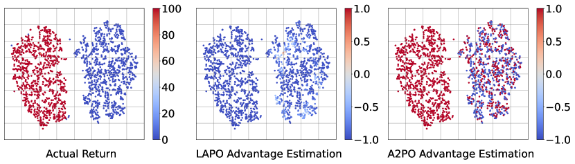
(a) walker2d-random-expert

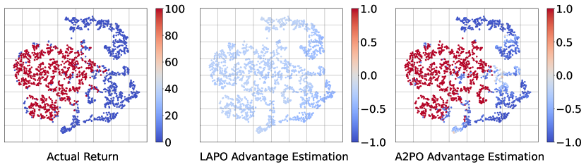
(b) hopper-random-expert

Figure 7: Comparison of our proposed A2PO method and the state-of-the-art AW method (LAPO) in advantage estimation for mixed-quality offline datasets (random-expert) in Gym tasks. Each data point represents an initial state-action pair in the offline dataset after applying PCA while varying shades of color indicate the magnitude of the actual return or advantage value.

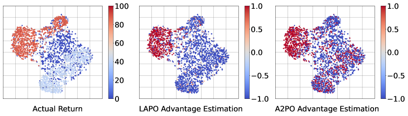
(a) halfcheetah-random-medium-expert

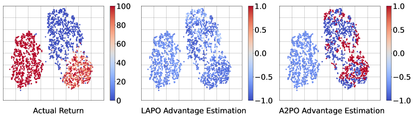
(b) walker2d-random-medium-expert

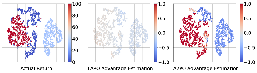
(c) hopper-random-medium-expert

Figure 8: Comparison of our proposed A2PO method and the state-of-the-art AW method (LAPO) in advantage estimation for mixed-quality offline datasets (random-medium-expert) in locomotion tasks. Each data point represents an initial state-action pair in the offline dataset after applying PCA while varying shades of color indicate the magnitude of the actual return or advantage value.

References

- Chebotar et al. (2023) Chebotar, Y., Vuong, Q., Irpan, A., Hausman, K., Xia, F., Lu, Y., Kumar, A., Yu, T., Herzog, A., Pertsch, K., et al. Q-transformer: Scalable offline reinforcement learning via autoregressive q-functions. arXiv preprint arXiv:2309.10150, 2023.
- Chen et al. (2021) Chen, L., Lu, K., Rajeswaran, A., Lee, K., Grover, A., Laskin, M., Abbeel, P., Srinivas, A., and Mordatch, I. Decision transformer: Reinforcement learning via sequence modeling. Advances in neural information processing systems, 34:15084–15097, 2021.
- Chen et al. (2020) Chen, X., Zhou, Z., Wang, Z., Wang, C., Wu, Y., and Ross, K. Bail: Best-action imitation learning for batch deep reinforcement learning. Advances in Neural Information Processing Systems, 33:18353–18363, 2020.
- Chen et al. (2022) Chen, X., Ghadirzadeh, A., Yu, T., Wang, J., Gao, A. Y., Li, W., Bin, L., Finn, C., and Zhang, C. Lapo: Latent-variable advantage-weighted policy optimization for offline reinforcement learning. Annual Conference on Neural Information Processing Systems, 35:36902–36913, 2022.
- Diehl et al. (2023) Diehl, C., Sievernich, T. S., Krüger, M., Hoffmann, F., and Bertram, T. Uncertainty-aware model-based offline reinforcement learning for automated driving. IEEE Robotics and Automation Letters, 8(2):1167–1174, 2023.
- Emmons et al. (2021) Emmons, S., Eysenbach, B., Kostrikov, I., and Levine, S. Rvs: What is essential for offline rl via supervised learning? arXiv preprint arXiv:2112.10751, 2021.
- Fu et al. (2020) Fu, J., Kumar, A., Nachum, O., Tucker, G., and Levine, S. D4rl: Datasets for deep data-driven reinforcement learning. arXiv preprint arXiv:2004.07219, 2020.
- Fujimoto & Gu (2021) Fujimoto, S. and Gu, S. S. A minimalist approach to offline reinforcement learning. Advances in neural information processing systems, 34:20132–20145, 2021.
- Fujimoto et al. (2018) Fujimoto, S., Hoof, H., and Meger, D. Addressing function approximation error in actor-critic methods. In International Conference on Machine Learning, 2018.
- Fujimoto et al. (2019) Fujimoto, S., Meger, D., and Precup, D. Off-policy deep reinforcement learning without exploration. In International Conference on Machine Learning, 2019.
- Gao et al. (2023a) Gao, C., Wang, S., Li, S., Chen, J., He, X., Lei, W., Li, B., Zhang, Y., and Jiang, P. Cirs: Bursting filter bubbles by counterfactual interactive recommender system. ACM Transactions on Information Systems, 42(1):1–27, 2023a.
- Gao et al. (2023b) Gao, C., Wu, C., Cao, M., Kong, R., Zhang, Z., and Yu, Y. Act: Empowering decision transformer with dynamic programming via advantage conditioning. arXiv preprint arXiv:2309.05915, 2023b.
- Ghasemipour et al. (2022) Ghasemipour, K., Gu, S. S., and Nachum, O. Why so pessimistic? estimating uncertainties for offline rl through ensembles, and why their independence matters. Annual Conference on Neural Information Processing Systems, 35:18267–18281, 2022.
- Hong et al. (2022) Hong, J., Kumar, A., and Levine, S. Confidence-conditioned value functions for offline reinforcement learning. arXiv preprint arXiv:2212.04607, 2022.
- Hong et al. (2023a) Hong, Z.-W., Agrawal, P., Combes, R. T. d., and Laroche, R. Harnessing mixed offline reinforcement learning datasets via trajectory weighting. arXiv preprint arXiv:2306.13085, 2023a.
- Hong et al. (2023b) Hong, Z.-W., Kumar, A., Karnik, S., Bhandwaldar, A., Srivastava, A., Pajarinen, J., Laroche, R., Gupta, A., and Agrawal, P. Beyond uniform sampling: Offline reinforcement learning with imbalanced datasets. In Thirty-seventh Conference on Neural Information Processing Systems, 2023b.
- Karabag & Topcu (2023) Karabag, M. O. and Topcu, U. On the sample complexity of vanilla model-based offline reinforcement learning with dependent samples. arXiv preprint arXiv:2303.04268, 2023.
- Kostrikov et al. (2021) Kostrikov, I., Nair, A., and Levine, S. Offline reinforcement learning with implicit q-learning. arXiv preprint arXiv:2110.06169, 2021.
- Kumar et al. (2019) Kumar, A., Fu, J., Soh, M., Tucker, G., and Levine, S. Stabilizing off-policy q-learning via bootstrapping error reduction. Annual Conference on Neural Information Processing Systems, 32, 2019.
- Kumar et al. (2020) Kumar, A., Zhou, A., Tucker, G., and Levine, S. Conservative q-learning for offline reinforcement learning. Advances in Neural Information Processing Systems, 33:1179–1191, 2020.
- Levine et al. (2020) Levine, S., Kumar, A., Tucker, G., and Fu, J. Offline reinforcement learning: Tutorial, review, and perspectives on open problems. arXiv preprint arXiv:2005.01643, 2020.
- Liu & Abbeel (2023) Liu, H. and Abbeel, P. Emergent agentic transformer from chain of hindsight experience. arXiv preprint arXiv:2305.16554, 2023.
- Lyu et al. (2022) Lyu, J., Ma, X., Li, X., and Lu, Z. Mildly conservative q-learning for offline reinforcement learning. Annual Conference on Neural Information Processing Systems, 35:1711–1724, 2022.
- Nair et al. (2020) Nair, A., Gupta, A., Dalal, M., and Levine, S. Awac: Accelerating online reinforcement learning with offline datasets. arXiv preprint arXiv:2006.09359, 2020.
- Paszke et al. (2019) Paszke, A., Gross, S., Massa, F., Lerer, A., Bradbury, J., Chanan, G., Killeen, T., Lin, Z., Gimelshein, N., Antiga, L., Desmaison, A., Kopf, A., Yang, E. Z., DeVito, Z., Raison, M., Tejani, A., Chilamkurthy, S., Steiner, B., Fang, L., Bai, J., and Chintala, S. Pytorch: An imperative style, high-performance deep learning library. In Annual Conference on Neural Information Processing Systems, 2019.
- Peng et al. (2019) Peng, X. B., Kumar, A., Zhang, G., and Levine, S. Advantage-weighted regression: Simple and scalable off-policy reinforcement learning. arXiv preprint arXiv:1910.00177, 2019.
- Peng et al. (2023) Peng, Z., Han, C., Liu, Y., and Zhou, Z. Weighted policy constraints for offline reinforcement learning. In AAAI Conference on Artificial Intelligence, 2023.
- Pomerleau (1991) Pomerleau, D. A. Efficient training of artificial neural networks for autonomous navigation. Neural Computation, 3(1):88–97, 1991.
- Prudencio et al. (2023) Prudencio, R. F., Maximo, M. R., and Colombini, E. L. A survey on offline reinforcement learning: Taxonomy, review, and open problems. IEEE Transactions on Neural Networks and Learning Systems, 2023.
- Puterman (2014) Puterman, M. L. Markov decision processes: discrete stochastic dynamic programming. John Wiley & Sons, 2014.
- Sakhi et al. (2023) Sakhi, O., Rohde, D., and Gilotte, A. Fast offline policy optimization for large scale recommendation. In AAAI Conference on Artificial Intelligence, 2023.
- Schulman et al. (2017) Schulman, J., Wolski, F., Dhariwal, P., Radford, A., and Klimov, O. Proximal policy optimization algorithms. arXiv preprint arXiv:1707.06347, 2017.
- Silver et al. (2014) Silver, D., Lever, G., Heess, N., Degris, T., Wierstra, D., and Riedmiller, M. Deterministic policy gradient algorithms. In International Conference on Machine Learning, 2014.
- Singh et al. (2022) Singh, A., Kumar, A., Vuong, Q., Chebotar, Y., and Levine, S. Offline rl with realistic datasets: Heteroskedasticity and support constraints. arXiv preprint arXiv:2211.01052, 2022.
- Sohn et al. (2015) Sohn, K., Lee, H., and Yan, X. Learning structured output representation using deep conditional generative models. Annual Conference on Neural Information Processing Systems, 28, 2015.
- Sutton & Barto (2018) Sutton, R. S. and Barto, A. G. Reinforcement learning: An introduction. MIT press, 2018.
- Tian et al. (2023) Tian, Q., Kuang, K., Liu, F., and Wang, B. Learning from good trajectories in offline multi-agent reinforcement learning. In AAAI Conference on Artificial Intelligence, 2023.
- Vuong et al. (2022) Vuong, Q., Kumar, A., Levine, S., and Chebotar, Y. Dasco: Dual-generator adversarial support constrained offline reinforcement learning. Annual Conference on Neural Information Processing Systems, 35:38937–38949, 2022.
- Wagenmaker & Pacchiano (2023) Wagenmaker, A. and Pacchiano, A. Leveraging offline data in online reinforcement learning. In International Conference on Machine Learning, 2023.
- Wang et al. (2023) Wang, S., Yang, Q., Gao, J., Lin, M. G., Chen, H., Wu, L., Jia, N., Song, S., and Huang, G. Train once, get a family: State-adaptive balances for offline-to-online reinforcement learning. arXiv preprint arXiv:2310.17966, 2023.
- Wang et al. (2022) Wang, Z., Hunt, J. J., and Zhou, M. Diffusion policies as an expressive policy class for offline reinforcement learning. arXiv preprint arXiv:2208.06193, 2022.
- Wu et al. (2022) Wu, J., Wu, H., Qiu, Z., Wang, J., and Long, M. Supported policy optimization for offline reinforcement learning. Annual Conference on Neural Information Processing Systems, 35:31278–31291, 2022.
- Xiao et al. (2022) Xiao, C., Wang, H., Pan, Y., White, A., and White, M. The in-sample softmax for offline reinforcement learning. In International Conference on Learning Representations, 2022.
- Xu et al. (2023) Xu, H., Jiang, L., Li, J., Yang, Z., Wang, Z., Chan, V. W. K., and Zhan, X. Offline rl with no ood actions: In-sample learning via implicit value regularization. arXiv preprint arXiv:2303.15810, 2023.
- Yamagata et al. (2023) Yamagata, T., Khalil, A., and Santos-Rodriguez, R. Q-learning decision transformer: Leveraging dynamic programming for conditional sequence modelling in offline rl. In International Conference on Machine Learning, pp. 38989–39007, 2023.
- Yang et al. (2023) Yang, J., Chen, X., Wang, S., and Zhang, B. Model-based offline policy optimization with adversarial network. arXiv preprint arXiv:2309.02157, 2023.
- Yu et al. (2020) Yu, T., Thomas, G., Yu, L., Ermon, S., Zou, J. Y., Levine, S., Finn, C., and Ma, T. Mopo: Model-based offline policy optimization. Annual Conference on Neural Information Processing Systems, 33:14129–14142, 2020.
- Zheng et al. (2023) Zheng, Q., Henaff, M., Amos, B., and Grover, A. Semi-supervised offline reinforcement learning with action-free trajectories. In International conference on machine learning, 2023.
- Zhou et al. (2021) Zhou, W., Bajracharya, S., and Held, D. Plas: Latent action space for offline reinforcement learning. In Conference on Robot Learning, 2021.
- Zhuang et al. (2023) Zhuang, Z., Lei, K., Liu, J., Wang, D., and Guo, Y. Behavior proximal policy optimization. arXiv preprint arXiv:2302.11312, 2023.