LISO: Lidar-only Self-Supervised 3D Object Detection

Abstract

3D object detection is one of the most important components in any Self-Driving stack, but current state-of-the-art (SOTA) lidar object detectors require costly & slow manual annotation of 3D bounding boxes to perform well. Recently, several methods emerged to generate pseudo ground truth without human supervision, however, all of these methods have various drawbacks: Some methods require sensor rigs with full camera coverage and accurate calibration, partly supplemented by an auxiliary optical flow engine. Others require expensive high-precision localization to find objects that disappeared over multiple drives.

We introduce a novel self-supervised method to train SOTA lidar object detection networks which works on unlabeled sequences of lidar point clouds only, which we call trajectory-regularized self-training. It utilizes a SOTA self-supervised lidar scene flow network under the hood to generate, track, and iteratively refine pseudo ground truth. We demonstrate the effectiveness of our approach for multiple SOTA object detection networks across multiple real-world datasets. Code will be released.

1 Introduction

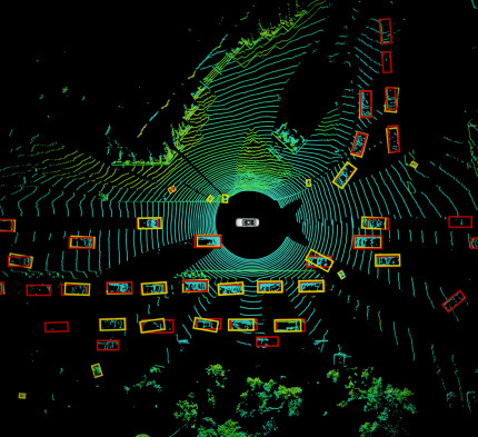
Figure 1: Objects predicted by our method using no manual annotations. Red boxes are ground truth boxes, yellow boxes are predicted by our network.

Human developmental research reveals that infants less than one year of age are able to categorize animate and inanimate objects based on observed motion cues and can generalize this categorization to previously unseen objects [24]. Yet, lidar object detectors with SOTA performance are trained using manually selected and categorized annotations. These annotations are very expensive to obtain and become outdated quickly: new lidar sensors are coming to market regularly, trained SOTA object detectors are sensitive to sensor characteristics and change in mounting position, and existing annotations are difficult to transfer between sensors or different sensor mounting positions [16], resulting in high re-labeling efforts with each change.

In this paper, we aim at bridging this gap by distilling motion cues observed in self-supervised lidar scene flow into SOTA single-frame lidar object detectors. We introduce a novel self-supervised method which is charmingly simple and easy to use: Input to our method are solely lidar pointcloud sequences. No human annotated bounding boxes, cameras, costly high-precision GPS, or tedious sensor rig calibration is required. Our method trains and runs a self-supervised lidar flow estimator [3] under the hood in order to create motion cues. We show in our experiments that these motion cues are a key factor to the success of our method. Based on the estimated lidar flow we bootstrap initial pseudo ground truth using simple clustering and track optimization. With these mined bounding boxes of moving objects we initialize a self-supervised, trajectory-regularized variant of self-training [1] (which is semi-supervised in its original form): We train a first version of a SOTA object detector, then iteratively re-generate and trajectory-regularize the pseudo ground truth and re-train the detector. Since the single-frame object detector has no concept of motion, it generalizes to detect any movable object on the way. Exemplary output of the trained detector, 3D boxes in single-frame point clouds, is depicted in Fig. 1.

Our contribution is a novel self-supervised  trajectory-regularized self-training framework for single-frame 3D object detection with the following properties:

• It is based entirely on lidar, i.e. without the limitations of prior works: no cameras, no calibration, no high-precision GPS, no manual annotations.

• It is agnostic w.r.t. the sensor model, mounting pose, and detectors architecture and works with the same set of hyper parameters: We demonstrate this across four different datasets and different SOTA detector networks.

• It is able to generalize from moving objects (motion cues) to movable objects (final detection results) and significantly outperforms SOTA methods while being simpler.

We show that using motion cues together with trajectory-regularized self-training is key to this success.

The code of this approach will be published for easy use and comparison by other researchers.

The paper is organized as follows: Sec. 2 discusses related work before the proposed method is described in detail in Sec. 3. Extensive experiments in Sec. 4 show the performance of our method before we conclude in Sec. 5.

2 Related Work

2.1 Single Frame Lidar 3D Object Detection

Object detectors operating on 3D point clouds are an active research field. The currently best-performing ones are using deep neural networks trained via supervised learning and can be categorized by their internal representation: Some networks operate on points directly like PointRCNN [19], 3DSSD [29], and IA-SSD [33]. Others project the points either to a virtual range image [12, 23, 11] or into a voxel representation like VoxelNet [34], PointPillars, CenterPoint [30], and Transfusion-L [2]. However, all aforementioned methods require large human-annotated datasets in order to perform well and obtaining such annotations is very expensive. We address this problem in this paper, enabling training of SOTA object detectors using pseudo ground truth.

2.2 Object Distilling from Motion Cues

Multiple approaches have been suggested which leverage motion cues from lidar frame pairs in order to detect moving objects. Using the assumption of local geometric constancy, they decompose dynamic scenes into separate moving entities by applying as-rigid-as-possible optimization. Examples of these are the works by Dewan et al. [6], RSF [5] and OGC [21]. The two former methods are optimization-based whereas OGC uses these constraints as loss-function to self-supervise a segmentation network.

Although these methods avoid the need for expensive labels, in contrast to our method they tend not to work well in low-resolution areas, they are typically slow, and can only detect moving but not movable (i.e. static but potentially moving) objects.

2.3 Pseudo Ground Truth for Object Detection

Different approaches have been proposed to mine pseudo ground truth for training object detectors: Najibi et al. [13] and very recently Seidenschwarz et al. [17] use motion cues similar to section 2.2 in order to distill moving objects as pseudo ground truth and use it to train an object detector. [13] runs optimization for each frame pair to obtain lidar scene flow, clusters points, fits boxes, tracks them using a Kalman Filter and finally refines them on ICP-registered point clouds. [17] optimizes a clustering algorithm on motion cues through message passing which they then apply to segment point clouds into a set of instances and subsequently fit boxes. As shown in [17], and in contrast to our approach, both methods suffer from a large performance gap between moving and movable objects. We demonstrate that our method does not suffer from this gap.

[10], [20] were the first to iteratively apply a detection, tracking, retraining paradigm to autonomous driving (AD) data. They build upon consistency constraints between object detectors which they train in the lidar and camera domain, making use of an optical flow network which is trained using supervision. The approach requires a calibrated sensor rig with possibly large camera coverage, IMU, and precision GPS. Similarly, [26] uses video sequences together with lidar scene flow to jointly train a camera and a lidar object detector. MODEST [31, 28] does not require coverage by calibrated cameras, but instead adds the additional requirement to have multiple lidar recordings of the same location in order to identify objects that vanished over time. With such demanding requirements, these approaches are not easy to use and are partially unsuited for popular AD datasets.

Oyster [32] is the approach most similar to ours. It uses DBSCAN [7] on lidar point clouds to initialize pseudo ground truth. Clusters are then tracked using forward-and-reverse tracking in sensor coordinates (i.e. without consideration for ego motion), using a complex policy for confidence-based track retention. After training an object detector on close range data, they employ zero-shot generalization to the far range data, track again and iteratively retrain the detector. In their experiments they use different hyperparameters for different datasets. Our method, in contrast, explicitly considers sensor motion, produces much cleaner initial proposals by leveraging a self-supervised lidar scene flow network, does not require zero-shot-generalization from near-to-far-field, and works with current SOTA object detectors. We show on multiple datasets that our method outperforms [32], that it works robustly with the same set of hyper-parameters and also generalizes well to detect movable objects. Additionally, we will release our code to facilitate further research on this topic.

3 Method

A general overview of our method is sketched in Fig. 2 and some steps illustrated in Fig. 3. As input, we take raw (unlabeled) point cloud sequences and undergo three stages, all of which are detailed in the following: Preprocessing of point clouds and lidar scene flow computation (Sec. 3.1), initial pseudo ground truth generation (Sec. 3.2) and repeated training with pseudo ground truth refinement (Sec. 3.3). The final output of the method is a trained object detector which can detect movable objects in raw single-frame point clouds.

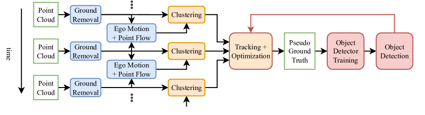
Figure 2: Overview of the proposed method. Point cloud sequences are preprocessed (blue, Sec 3.1), initial pseudo ground truth is created (orange, Sec. 3.2) and the object detector is iteratively trained and pseudo ground truth regenerated (red, Sec. 3.2).

3.1 Preprocessing

We preprocess the raw input point clouds as follows:

Ground Removal: First, we remove distracting ground points from each single point cloud using JCP [18], which is a simple, robust, yet effective algorithm to remove ground points using changes in observed height above ground.

Ego Motion Estimation: Second, we compute ego-motion between neighboring frame pairs using KISS-ICP [25], which is based on a robust version of ICP. The output is a cm-level accurate transformation $\mathbf{T}_{\text{ego}}^{t\rightarrow t+1}\in\mathbb{R}^{4\times 4}$, describing the ego vehicle position at time $t+1$ represented in the ego frame from time $t$.

Lidar Scene Flow Estimation: Third, we compute lidar scene flow between neighboring frame pairs resulting in a flow vector $\mathbf{f}_{i}=(dx,dy,dz)$ for every point $i$ in the first point cloud $\mathcal{P}^{t}$. We chose to use SLIM [3] as its code is readily available, it is easy to use, features fast inference, and produces SOTA results. The network is trained self-supervised on raw point cloud sequences, minimizing a k-nearest-neighbor loss between forward and time-reversed point clouds.

The components of our preprocessing steps (Ground Removal, Ego Motion Estimation, Lidar Scene Flow Estimation) have been selected for robustness and are all used with their default parameters from their respective publications.

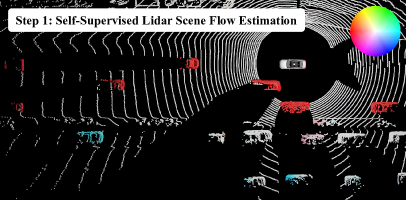
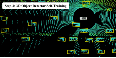
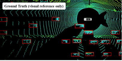
Figure 3: Overview over preprocessing, initial pseudo ground truth generation and training with examples. Top left: In the first step, self-supervised lidar scene flow is computed and corrected for vehicle ego-motion. Points are colored by flow direction and magnitude. Top right: In the second step, the scene flow is clustered and bounding boxes are fitted (to the moving objects). Bottom left: In the third step, the network is trained on the pseudo ground truth and is generalizing to static objects also, since it does not have the motion information as input signal. Points are thus colored by laser intensity. Bottom right: Ground truth, for reference.

3.2 Initial Pseudo Ground Truth Generation

The aim of our method is to mine pseudo ground truth for training a 3D lidar object detector. For a single point cloud $\mathcal{P}^{t}$ (consisting of $n\in\mathbb{N}$ points $\mathbf{p}_{i}$, $\mathbf{p}_{i}\in\mathcal{P}^{t}$) this ground truth is a set of 3D bounding boxes $\mathcal{B}$ with confidences representing the objects at time $t$:

$$\mathcal{B}^{t}=\{\text{B}^{t}_{j},j\in\mathbb{N}\}=\{(x,y,z,l,w,h,\theta,c)_{j}\}$$ (1)

Here, $(x,y,z)=\mathbf{x}$ define the center position, $(l,w,h)$ the length, width and height, $\theta$ the heading (orientation around up axis), and $c$ the confidence for a single box.

The key success factor of our method is to focus on a high precision (and potentially low recall) of the initial set of bounding boxes in order to avoid "wrong" objects to negatively influence the object detector. We achieve this by leveraging shape, density, and especially motion cues to robustly identify moving objects solely (see also top-right of Fig. 3). Sec. 3.3 targets at generalizing these to movable objects later on.

Flow Clustering: The points $\mathbf{p}_{i}\in\mathcal{P}^{t}$ in each preprocessed point cloud are clustered based on geometry and motion: All stationary points in a scene should have a flow $\mathbf{f}_{i}$ similar to the vehicle’s ego-motion, i.e. $\mathbf{f}_{i}\approx\mathbf{f}_{i,\text{sta}}=((\mathbf{T}_{\text{ego}}^{t\rightarrow t+1})^{-1}-\mathbf{I}_{4})\cdot\mathbf{p}_{i}$. The residual flow must then be caused by motion of other actors: $\mathbf{f}_{i,\text{dyn}}=\mathbf{f}_{i}-\mathbf{f}_{i,\text{sta}}$. We filter all static points by applying a threshold of 1$\mathrm{m}\mathrm{/}\mathrm{s}$ to the residual flow and cluster the remaining points based on their point location and flow vector in 6D using DBSCAN [7](with parameters $\varepsilon=1.0$, $\text{minPts}=5$).

We fit a 3D bounding box $\text{B}^{t}_{j}$ to each resulting cluster following [31] and discard boxes with $l/w>4.0$, $lw<0.35$\mathrm{m}$^{2}$, or $lwh<0.5$\mathrm{m}$^{3}$. The heading $\theta$ is set to match the "forward-axis" of the motion, i.e. we orient the boxes along the direction of the residual flow $\mathbf{f}_{i,\text{dyn}}$. The confidence $c$ is set to 1.

Tracking: We run a simple flow based tracker: Since we have accurate ego-motion available, we can track accurately in a fixed coordinate system w.r.t. the world. First, using the residual flow, we can compute for each box at $t$ a rigid body transform that transforms the proposed box $\text{B}_{i}^{t}$ forward in time towards its suspected location at $t+1$, $\hat{\text{B}}_{i}^{t+1}$. The propagated boxes $\hat{\mathcal{B}}^{t+1}$ are matched greedily against the actual boxes $\mathcal{B}^{t+1}$ based on box-center distance to the new detections. Unmatched boxes in $\mathcal{B}^{t+1}$ which are further away than 1.5m from propagated boxes spawn new tracklets. Unmatched tracklets from $\mathcal{B}^{t}$ are propagated according to the last observed box motion for up to one time step, after that unmatched tracklets are terminated. We run tracking forward and reverse in time, connecting tracklets from forward and reverse tracking to tracks.

The resulting set of tracks is post-filtered: We discard tracks that are shorter than 4 time steps or that have a median box confidence $c$ lower than threshold $0.3$ (note that the initial confidence $c=1$ set during clustering is later replaced by detectors confidences, see Sec. 3.3). This retains only stable and high-confident tracks and avoids false positives to enter the pseudo ground truth.

Track Optimization: We reduce positional noise of the tracks by minimizing translational jerk on all tracks longer than 3$\mathrm{m}$. Let $\mathcal{X}_{\text{obs}}$ be the sequence of (noisy) observed box center positions $\mathbf{x}_{i}$ for consecutive time steps $i\in\{1,...,T\}$ of a track and their derivative $\frac{d\mathbf{x}_{i}}{dt}\approx\frac{\mathbf{x}_{i+1}-\mathbf{x}_{i}}{\Delta t}$. We compute smoothed track positions $\mathcal{X}_{\text{smooth}}$ by initializing them to $\mathcal{X}_{\text{obs}}$ and minimizing the following loss w.r.t. $\mathbf{x}_{\text{smooth}}$:

$$L=\sum_{i=1}^{T}\left\|\frac{d^{4}\mathbf{x}_{i,\text{smooth}}}{dt^{4}}\right\|_{2}^{2}+\beta\left\|\mathbf{x}_{i,\text{smooth}}-\mathbf{x}_{i,\text{obs}}\right\|_{2}^{2}$$ (2)

I.e. we minimize the jerk $\frac{d^{4}\mathbf{x}}{dt^{4}}$ and use a quadratic regularizer term ($\beta=3$) on the positions. Experiments revealed that this simple optimization goal outperforms more sophisticated ones like fitting an unrolled bicycle model or adding terms for acceleration, which leads to tracks "overshooting" corners, especially when using aggressive optimization parameters required to run at reasonably fast optimization time.

We subsequently align the orientation $\theta$ of each detection in a track to the direction of the smoothed track at its position. Box dimensions $\{l,w,h\}$ of all boxes in a track are adapted to the 90 percentile of observed box dimensions in a track. All hyperparameters related to clustering, tracking and track optimization have been tuned visually on two sample snippets from nuScenes.

3.3 Trajectory-Regularized Self-Training

After having mined initial pseudo ground truth of moving objects with a high precision and low recall, we now aim at iteratively improving our pseudo ground truth by training and using an object detector so that the pseudo ground truth generalizes to movable objects. We achieve this by executing iterative trajectory-regularized self-training, which is composed of the following two steps:

Training: We train the target object detection network using the current pseudo ground truth in a supervised training setup. Any single-frame object detection network can be plugged into our pipeline. In our experiments we do not deviate from the basic training setup of our object detection networks. Like any SOTA object detection method, we apply standard augmentation techniques to a point cloud during network training: Random rotation, scaling ($\pm 5\%$), and random translation up to $5$\mathrm{m}$$ around the origin. Furthermore, we randomly pick 1 to 15 objects from the pseudo ground truth database and insert a random subset of their points at random locations into the scene.

Pseudo Ground Truth Regeneration: After a certain amount of training steps ($s=30k$ in the experiments) we stop the training and use the trained object detector to recreate new, improved pseudo ground truth: We run the trained detector in inference mode over all sequences in the training dataset to generate new box detections $\mathcal{B}$, thereby using the detectors’ confidence as box confidence $c$. We regularize these detections by running the flow-based tracker and track smoothing exactly like we do for the initial pseudo ground truth generation. Every $2nd$ iteration (i.e. every $60k$ steps in the experiments), we discard the network weights after regenerating the pseudo ground truth.

Fig. 4 illustrates the effect of our self-training: We see that the pseudo ground truth improves with each re-generation and that dropping network-weights allows the network to re-focus on the generalized pseudo ground truth. The pseudo ground truth has a consistently lower performance because we keep it conservative, keeping only highly certain boxes.

Two aspects are key to making our method perform well:

• Being restrictive when composing the pseudo ground truth (i.e. using plausible tracks of high-confidence network detections or clusters with significant flow only) avoids adding false positives into the pseudo ground truth and hence avoids that our network increasingly hallucinates with each iteration.

• Not using flow but only single-frame pointclouds as input for the detector allows the detector to focus on appearance of objects solely.

These allow our method to generalize from initially mined moving objects to movable objects in the scene.

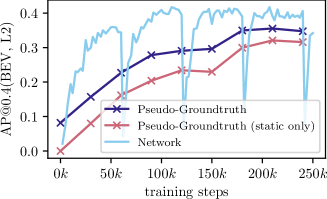
[Effect of self-supervised self-learning] [Evaluation of Self-Training Hyperparameters]

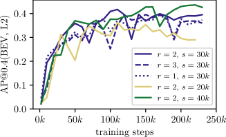
Figure 4: Left: Effect of self-supervised self-learning: At the beginning of the training, only moving objects are contained within the pseudo ground truth and the pseudo ground truth thus scores 0 on static objects. Thanks to the self-training, the network generalizes to movable objects and the score of the pseudo ground truth on static objects starts to increase with every regeneration at each ”X”. The pseudo ground truth’s performance is measured on a subset of the train set of WOD dataset, while the network (here: Centerpoint) is evaluated on a small subset of the validation set. Right: Evaluation of Self-Training Hyperparameters: Network (Centerpoint) performance over the course of a training on WOD. $s$ is the number of training steps between pseudo ground truth regenerations, $r$ is the number of regenerations after which network weights are dropped and re-initialized.

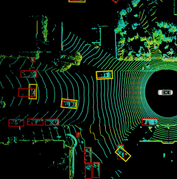
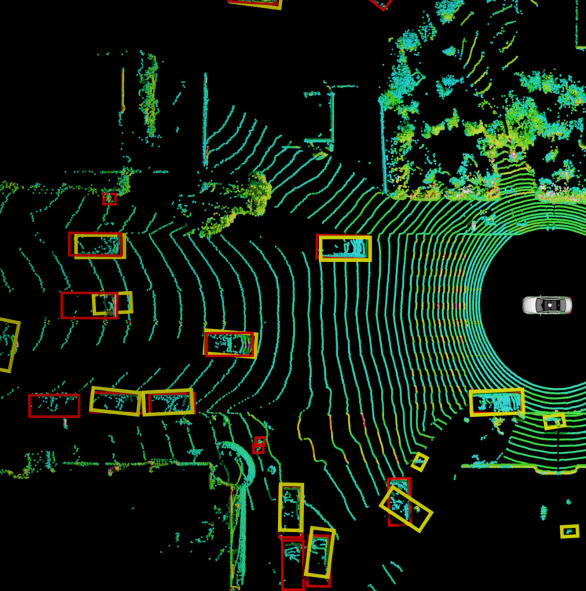
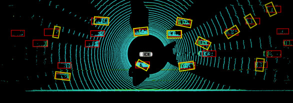
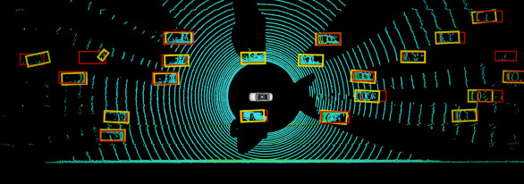
Figure 5: Qualitative Results on WOD. Red boxes are ground truth boxes, yellow are predictions. Left: OYSTER-CP Right: LISO-CP

4 Evaluation

We evaluate our method on multiple datasets across multiple SOTA networks. SLIM [3], the self-supervised flow network we use, is trained and inferred as in the published version, but Bird’s-Eye-View (BEV) range is extended from $70\times 70$\mathrm{m}$$, $640\times 640$ pixels to $120\times 120$\mathrm{m}$$ and $920\times 920$ pixels.

		AV2				nuScenes
		BEV-IOU		3D-IOU
		AP@0.3$\uparrow$	AP@0.5$\uparrow$	AP@0.3$\uparrow$	AP@0.5$\uparrow$	AP$\uparrow$	AOE$\downarrow$
Sup.	CP[30]	0.778	0.778	0.736	0.517	0.484	0.560
	TF[2]	0.783	0.654	0.767	0.601	0.627	0.501
Unsupervised	DBSCAN[7]	0.054	0.026	0.020	0.003	0.008	3.120
	DBSCAN(SF)	0.070	0.026	0.065	0.015	0.003	2.623
	DBSCAN(GF)	0.105	0.041	0.088	0.024	0.000	1.000
	RSF[5]	0.074	0.026	0.055	0.014	0.019	1.003
Self Train	Oyster[32] ${\dagger}$	0.354	0.245	-	-	-	-
	Oyster-CP[32]	0.381	0.266	0.150	0.002	0.091	1.514
	Oyster-TF[32]	0.340	0.198	0.182	0.016	0.093	1.564
	LISO-CP	0.448	0.335	0.367	0.188	0.109	1.062
	LISO-TF	0.417	0.294	0.317	0.176	0.134	0.938

Table 1: Evaluation on AV2 [27] and nuScenes[4]: CP, TF: network architecture, in the first two lines trained supervised for comparison. ${\dagger}$: Metrics as reported in [32]. SF: self-supervised lidar scene flow by SLIM, GF: ground truth lidar scene flow. Note that nuScenes uses a minimum precision and recall threshold of 0.1, and since the recall of GT flow clustering is lower than 0.1, all results are clipped away. For full nuScenes scores see supplementary material.

		Movable		Moving		Still		Vehicle	Pedestrian	Cyclist
		AP@0.4$\uparrow$		AP@0.4$\uparrow$		AP@0.4$\uparrow$		AP@0.4 $\uparrow$	AP@0.4 $\uparrow$	AP@0.4 $\uparrow$
		BEV	3D	BEV	3D	BEV	3D	BEV	BEV	BEV
Sup.	CP[30]	0.765	0.684	0.721	0.624	0.735	0.657	0.912	0.513	0.134
	TF[2]	0.746	0.723	0.714	0.668	0.733	0.710	0.918	0.457	0.216
Unsupervised	DBSCAN[7]	0.027	0.008	0.009	0.000	0.027	0.006	0.184	0.002	0.001
	DBSCAN(SF)	0.026	0.010	0.064	0.041	0.000	0.000	0.073	0.010	0.009
	DBSCAN(GF)	0.114	0.071	0.318	0.120	0.000	0.000	0.113	0.111	0.240
	RSF[5]	0.030	0.020	0.080	0.055	0.000	0.000	0.109	0.000	0.002
	SeMoLi [17] $\dagger$	-	0.195	-	0.575	-	-	-	-	-
	LISO-CP	0.292	0.211	0.272	0.204	0.208	0.140	0.607	0.029	0.010
Self Train	Oyster-CP[32]	0.217	0.084	0.151	0.062	0.176	0.056	0.562	0.000	0.000
	Oyster-TF[32]	0.121	0.015	0.051	0.007	0.098	0.010	0.475	0.000	0.000
	LISO-CP	0.380	0.308	0.350	0.296	0.322	0.255	0.695	0.055	0.022
	LISO-TF	0.327	0.208	0.349	0.245	0.233	0.126	0.669	0.024	0.012

Table 2: Evaluation on WOD dataset: We evaluate using the protocol of [17, 13], using an area of whole 100$\mathrm{m}$$\times$40$\mathrm{m}$ BEV grid around the ego vehicle, considering objects that move faster than 1$\mathrm{m}\mathrm{/}\mathrm{s}$ to be moving (difficulty level L2). CP, TF: network architecture, in the first two lines trained supervised for comparison. $\dagger$: Results taken from [17]. SF: lidar scene flow by SLIM, GF: ground truth lidar scene flow. For class-specific 3D detection scores see supplementary material.

	Movable (Moving & Still)				Car		Pedestrian		Cyclist
	BEV-IOU		3D-IOU		BEV-IOU		BEV-IOU		BEV-IOU
	AP@0.3$\uparrow$	AP@0.5$\uparrow$	AP@0.3$\uparrow$	AP@0.5$\uparrow$	AP@0.3$\uparrow$	AP@0.5$\uparrow$	AP@0.3$\uparrow$	AP@0.5$\uparrow$	AP@0.3$\uparrow$	AP@0.5$\uparrow$
CP [30]	0.755	0.690	0.736	0.601	0.814	0.794	0.370	0.128	0.409	0.157
TF [2]	0.747	0.665	0.729	0.582	0.820	0.776	0.311	0.096	0.263	0.032
DBSCAN[7]	0.023	0.002	0.010	0.000	0.026	0.005	0.000	0.000	0.064	0.007
RSF [5]	0.029	0.019	0.029	0.011	0.066	0.049	0.000	0.000	0.192	0.043
Oyster-CP[32]	0.235	0.098	0.114	0.000	0.327	0.135	0.000	0.000	0.000	0.000
Oyster-TF[32]	0.273	0.088	0.128	0.000	0.364	0.121	0.000	0.000	0.019	0.000
LISO-CP	0.446	0.330	0.419	0.159	0.520	0.411	0.097	0.019	0.445	0.053
LISO-TF	0.361	0.207	0.294	0.036	0.425	0.297	0.084	0.014	0.348	0.003

Table 3: Evaluation on KITTI dataset: We evaluate on the forward facing field of view where GT annotations are available, but run inference on the whole $100\times 100$\mathrm{m}$$ BEV grid. Also note that flow annotations are not available for KITTI Object. CP, TF: network architecture, in the first two lines trained supervised for comparison.

4.1 Datasets and Metrics

We evaluate our method on four different AD datasets. For a fair comparison, we compute metrics for movable objects by mapping all animate objects (Cars, Trucks, Trailers, Motorcycles, Cyclists, Pedestrians and other Vehicles) to a single category and discarding all inanimate objects (Barrier, Traffic Cone,…) since our method does not predict any class attributes. In Table 2 and Table 3 we also give class-based results for completeness. Class labels for true positives are taken from ground truth. For false positives, the predicted class label is assigned randomly according to the label distribution in the dataset.

Waymo Open Dataset (WOD): [22] is a large, geographically diverse dataset recorded with a proprietary high quality lidar. We evaluate using the protocol of [13, 17], using an area of whole 100m$\times$40m BEV grid around the ego vehicle, artificially cropping the predictions of our method down to this reduced area.

KITTI: [9, 8] is recorded using a Velodyne HDL64 lidar sensor, where some parts have been annotated with 3D object boxes and tracking information in the forward facing camera field of view. A large portion of the published data is only available in raw format without annotations, which our method is able to leverage, due to not requiring any ground truth annotations for training.

Argoverse 2: AV2 [27] is recorded using two stacked Velodyne VLP32 lidar sensors and annotated with 3D object boxes. On AV2 and KITTI, we evaluate both 2D (in BEV space) and 3D box IoU at IoU thresholds of 0.3 and 0.5 in the area of $100\times 100$\mathrm{m}$$ around the ego vehicle.

nuScenes: [4] is recorded using a Velodyne VLP32 lidar sensor. We evaluate using the nuScenes protocol. Please note that models trained with our method get a high penalty on the Nuscenes Detection Score (NDS), because they cannot distinguish object classes and therefore score an Average Attribute Error of 1.0.

4.2 Networks

We evaluate our proposed method with two SOTA lidar object detection networks of different architecture: Centerpoint [30] and Transfusion-L [2]. For both we do not make any modification to the published implementation or network architecture or losses. We train both networks with a batch size of four.

CenterPoint: [30] is based on 2D convolutions in BEV space. Object centers are represented as heatmap in the BEV, which are then reduced to a sensible amount of boxes using non-maximum-suppression.

Transfusion-L: [2] is a Transformer based architecture, which is applied after initial encoding of the LiDAR point cloud into a 2D BEV feature tensor.

4.3 Baselines

Besides the obvious baseline of training the object detection networks supervised from scratch on ground truth from the dataset, we also compare to multiple strong unsupervised baselines. For details, see Sec. 2.

RSF: We include RSF [5] in our evaluation as strong representative of methods doing object distilling from motion cues. We ran experiments using the published code of the authors.

DBSCAN: This algorithm [7] clusters points in the point cloud with similar 3D locations into objects. We additionally evaluate extending the cluster space to 6D by either using SLIM scene flow (SF) or ground-truth scene flow (GT). Thus, the "DBSCAN(SF)" baseline essentially corresponds to the raw detections used for our initial pseudo ground truth generation. We use the implementation from [15] with parameter values 1.0 for epsilon and 5 for the minimum number of points for a valid cluster.

SeMoLi: [17] is the most recent baseline. As it showed to outperform [13] as self-supervised object detection method we include only published results of [17] in our evaluation.

Oyster: We reimplemented [32] using PyTorch [14], and apply the proposed framework to the used networks CenterPoint and Transfusion-L (abbreviated Oyster-CP and Oyster-TF) to be as close as possible to our method and evaluation. We verify our re-implementation, by reproducing the reported metrics by [32] on AV2, see Table 1.

4.4 Results

Quantitative Results: On all four datasets we see that our method consistently outperforms all self-supervised baselines in all metrics for movable objects, see Table 1, Table 2, and Table 3. Only SeMoLi[17] beats LISO on moving objects (see Table 2) but significantly drops below LISO’s performance on movable objects, hinting to difficulties with generalization. Our method does not suffer from this performance gap and performs nearly equally well on movable and moving objects. We also observe that, despite mostly better performance in the supervised case, Transfusion-L responds less favorable than Centerpoint to the self-supervised training approaches. We suspect that Centerpoint, due to its convolutional architecture and its lack of positional encoding compared to Transfusion-L, is less susceptible to overfitting to where moving objects have been observed and where not to expect them.

We also observe that the nuScenes dataset seems to be the most challenging for the self-supervised methods, leading to the biggest gap between supervised and unsupervised object detection performance. We attribute this to the sparseness of the lidar sensor used in the dataset with only 32 layers. Common to all self-supervised methods is the difficulty in estimating the forward orientation of objects (AOE on nuScenes, $2\pi$ periodic, see Table 1), which the pure IoU based metrics cannot reveal.

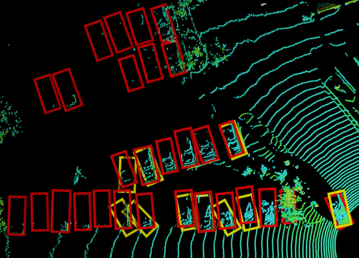
Figure 6: Missed ground truth boxes in the WOD dataset.

Qualitative Results: In Fig. 5 we compare our method to the best-performing baseline, Oyster, using Centerpoint as network architecture. It can be seen, that our method has higher accuracy and especially predicts box orientations more accurately.

Fig. 6, in contrast, showcases an important failure-case and general problem of all unsupervised methods: ground truth, especially in the WOD dataset, is also annotated in very sparse and distant regions. It is very challenging to generate pseudo ground truth for such regions whereas supervised trainings do not have to generalize from moving to such movable (but very sparse) objects. This may be the main reason for a still noticeable gap in evaluation results between supervised and unsupervised methods.

4.5 Ablation Study

We investigated the influence of different choices for the components in our pipeline, see Table 4 and cf. Fig. 2.

Motion Cues as Clustering Input: When adding motion cues to box clustering for Oyster we observe that detection performance already increases noticeably (comparing #3 to #4, Table 4). This demonstrates that self-supervised motion cues are a key ingredient to get high-quality initial pseudo ground truth as opposed to just using clustered 3D points.

Tag	Cluster Input	Method	Self Train	Track Optim.	AP@0.4(BEV)	AP@0.4(3D)
#1	P, SF	no tracker			0.177	0.086
#2	P, SF	no tracker	✓		0.201	0.131
#3	P	Oyster	✓		0.217	0.084
#4	P, SF	Oyster	✓		0.255	0.104
#5	P, SF	LISO(K, SF)			0.279	0.209
#6	P, SF	LISO(K, SF)	✓		0.360	0.290
#7	P, SF	LISO(K, SF)		✓	0.292	0.211
#8	P, SF	LISO(K, SF)	✓	✓	0.380	0.308
#9	P, SF	LISO(G, SF)	✓	✓	0.411	0.339
#10	P, GF	LISO(G, GF)	✓	✓	0.423	0.349

Table 4: Ablation study of different parts of our pipeline on WOD with Centerpoint [30]. Abbreviations: P: points, SF: self-supervised lidar scene flow (SLIM), GF: ground truth lidar scene flow. K: KISS-ICP ego-motion, G: ground truth ego-motion.

Motion Cues for Tracking: Our lidar scene flow-based tracker is the biggest contributing factor to the success of our method: the ablation reveals that leveraging motion cues greatly improves tracking (comparing #4 to #6) and thus ultimately improves self-training, i.e. more accurate tracking allows for much more strictness when matching and filtering tracklets. (The Oyster tracker uses a matching threshold of $5$\mathrm{m}$$, our threshold is only $1.5$\mathrm{m}$$). This strictness leads to higher quality pseudo ground truth.

Effect of Self Training: Even without using any tracker to filter tracklets self training has a benefit (comparing #1 to #2). This is due to the network generalizing to new instances and confidence thresholding the detections. However, having an additional way to discard implausible detections (by tracking) amplifies the positive effect of self training (comparing #5 to #6 and #7 to #8), as it can better prevent false positives from entering the pseudo ground truth.

Track Optimization: The added benefit of Track Optimization is more independent of Self Training (comparing going from #5 to #7 with going from #6 to #8). Finally we notice, that with the combination of a strict tracker, track optimization and self training, the performance is very close to using ground truth flow and ego-motion (comparing #8 to #9 and #10).

Hyperparameters for Iterative Training: Fig. 4 demonstrates that the performance of our proposed method is relatively consistent across a range of hyperparameters. However, using too few steps between regeneration of pseudo ground truth ($s=20k$) leads to degrading performance, because the network does not have enough time to generalize and stabilize using the pseudo ground truth, which then has negative effects during regeneration of the pseudo ground truth. The experiment reveals that doing multiple iterations of self-learning and dropping network-weights to allow the network to adjust is beneficial for a good performance. We selected $r=2$ and $s=30k$ as a good compromise between performance and speed for all other experiments.

5 Conclusion

We have proposed a novel framework for self-supervised 3D lidar object detection based on self-supervised lidar scene flow. Using simple clustering on lidar scene flow in combination with a novel flow-based tracker, we were able to generate pseudo ground truth with moving objects at high precision. This enabled us to bootstrap SOTA 3D lidar object detectors, without using any human labels. The detector generalizes from detecting moving to detecting movable objects over multiple self-training iterations. Experiments revealed that our trajectory-regularized self-learning, based on our scene flow-based tracker, is key to the success of our method. We have demonstrated the effectiveness of our approach on two SOTA lidar object detectors as well as four AD datasets. All experiments were conducted with the same set of hyperparameters, demonstrating the robustness of our method. Our method achieves a significant improvement in the state-of-the-art of self-supervised lidar object detection on all four datasets. Code will be released.

The biggest limitation of our approach is that our method is not able to distinguish different classes. Future work could be around generating pseudo ground truth for class labels, e.g. based on motion or size characteristics.

Supplementary Material

Appendix 0.A Implementation Details

We run the networks Centerpoint [30] and Transfusion-L [2] on $100\times 100$\mathrm{m}$$ BEV grids around the ego vehicle. We use non-maximum suppression with a threshold of $0.1$ (2D BEV IoU) for the detections. The optimizers, as well as their learning rate schedules are kept from the respective original implementations, but the schedules are shortened to match the lifecycle of the network weights during the iterative rounds of self-training. For the zero-shot generalization required by Oyster [32] after the first round, we found that starting from an initial BEV range of $50\times 50$\mathrm{m}$$, and then extending to $100\times 100$\mathrm{m}$$, gave the best results. For DBSCAN we used $\varepsilon=1.0$, and $\text{minPts}=5$. We optimize all tracks using Adam optimizer with learning rate 0.1 for 2000 steps for a complete point cloud sequence batched (at the same time), which takes less than 2$\mathrm{s}$ per nuScenes session on a Nvidia V100 GPU.

Appendix 0.B Self-supervised lidar scene flow

Train Data	Val Data	AEE(moving)[m] $\downarrow$	AEE(static)[m]$\downarrow$
AV2 Train	AV2 Val	0.075	0.079
KITTI Raw	KITTI Tracking	0.092	0.104
nuScenes Train	nuScenes Val	0.132	0.077
WOD Train	WOD Val	0.091	0.085

Table 5: Lidar scene flow metrics of SLIM [3] on the datasets (evaluated on val split), for a BEV range of $\mathbf{120\times 120$\mathbf{\mathrm{m}}$}$. Note that for KITTI, we only evaluate the forward-facing FoV which has been annotated with tracked objects. Objects faster than $1$\mathrm{m}\mathrm{/}\mathrm{s}$$ are considered moving. AEE refers to the average endpoint error across either all moving or static points.

As mentioned in Sec. 4, we extend the BEV range of SLIM [3] from $70\times 70$\mathrm{m}$$, $640\times 640$ pixels to $120\times 120$\mathrm{m}$$ and $920\times 920$ pixels, but make no further modifications to the network. This results in the SOTA scene flow quality described in Table 5.

The small performance gap of our method between using ground truth and SLIM lidar scene flow (comparing the last and the second-to-last row of Table 4) demonstrates that SLIM lidar scene flow has suitable quality for our method, and also that our method does not require absolutely perfect lidar scene flow estimates to work well. Ground truth lidar scene flow is generated using the recorded vehicle egomotion for static points and the tracking information (bounding boxes) of moving objects.

Appendix 0.C Performance of lidar scene flow clustering on nuScenes

In the evaluation on nuScenes (see Table 6), the worse performance of using DBSCAN [7] clustering on ground truth lidar scene flow compared to using DBSCAN on SLIM lidar scene flow is surprising.

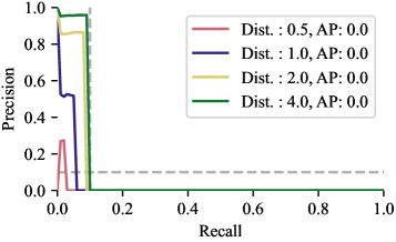
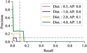
Figure 7: Performance comparison of clustering ground truth lidar scene flow(top) and SLIM [3] lidar scene flow (bottom) on the nuScenes dataset. The methods are evaluated according to the official nuScenes protocol on the validation split. The dashed line represents the minimum threshold for precision and recall of $0.1$, all results below these two thresholds are discarded. This leads to the surprising effect that the AP score is higher when using SLIM lidar scene flow, but this is only a result of the clipping dictated by the nuScenes evaluation protocol.

However, this peculiar effect is explained by Fig. 7, which shows the full precision-recall curves, generated using the official nuScenes protocol on the validation split [4]. The nuScenes protocol uses minimum precision and recall value thresholds of $0.1$, discarding all results below these thresholds. As mentioned in Section 3.2, we assign confidence score of $1.0$ to all clusters discovered by DBSCAN. This causes all detections generated using DBSCAN on ground truth lidar scene flow to be discarded.

Appendix 0.D Quality of pseudo ground truth during Iterative Self-Training

One critical aspect of iterative self-training is the quality of pseudo ground truth on the training dynamics, as depicted in Fig. 8. Finding the right balance between precision and recall in the pseudo ground truth is crucial for achieving optimal performance during self-training iterations: In our experiments, we find that having initially a small subset of high precision training samples is superior to having a larger set with higher recall but worse precision, because it allows the model to learn from a smaller but more reliable set of labeled data. A larger set of pseudo ground truth that is collected with less rigorous clustering, tracking and filtering, includes more noisy and mislabeled data. As discussed in [32, 31], the limited model capacity does prevent the model from overfitting to the inconsistent noises in the pseudo ground truth to some extent and the model generalizes mostly to the objects of interest [32, 31], but in our experiments, higher quality pseudo ground truth with less noise ultimately leads to better performance. Motion cues (i.e. egomotion and lidar scene flow) are the superior clustering and tracking input signal, allowing our method to generate much cleaner initial pseudo ground truth when compared to Oyster, which we also demonstrate in our ablation in Table 4. Fig. 9 additionally visually demonstrates the difference between using lidar scene flow for initial pseudo ground truth creation and just using point clouds (Oyster) on an example point cloud: As expected, using lidar scene flow leads to fewer false positives in the initial pseudo ground truth.

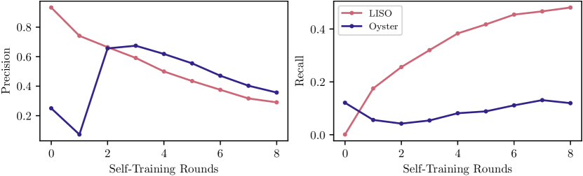
Figure 8: Precision and recall of the (tracked) pseudo ground truth generated by Oyster and LISO over the course of self-training of Centerpoint on WOD (training split). Precision and recall are computed like in the AP metrics used in Fig. 4 and Table 2, i.e. true positives are occurences where the BEV IoU between ground truth and predicted boxes is greater than 0.4, but at a specific confidence threshold: For Oyster, we use the reported value from the publication $c=0.4$ [32]. For LISO, we use $c=0.3$ and only discard the learned weights every other round, as stated in Section 3.2. Note that the dip in Oyster’s performance at round 1 stems from the zero-shot generalization, where the network is tasked to generalize from the training on the initial pseudo ground truth generated on the smaller BEV range to the full, previously unseen BEV range, going from $50\times 50$\mathrm{m}$$ to $100\times 100$\mathrm{m}$$.

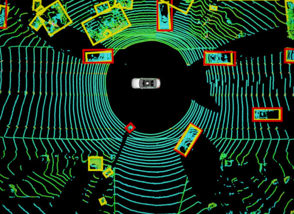
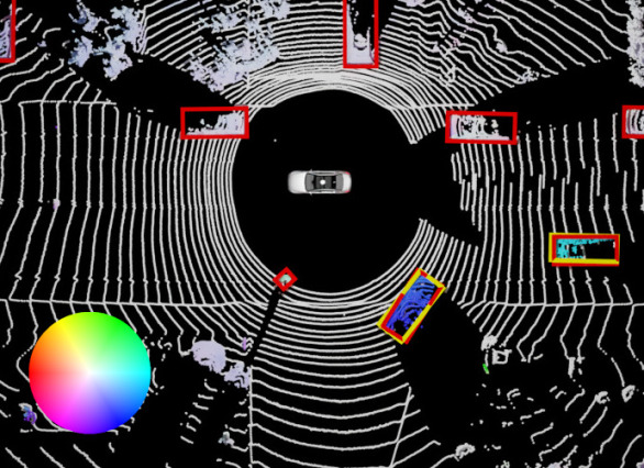
Figure 9: Clustering results for the initial pseudo ground truth generation on WOD. Red boxes are ground truth boxes, yellow are predictions. Left: Oyster Clustering result on points, with high recall but low precision. Right: LISO Clustering result on points and SLIM lidar scene flow, resulting in in high precision pseudo ground truth (LISO). Points are colored according to flow direction and magnitude.

Appendix 0.E Qualitative Results

For more qualitative comparisons besides Fig. 10 or Fig. 5, we kindly refer the reader to the video accompanying this supplement.

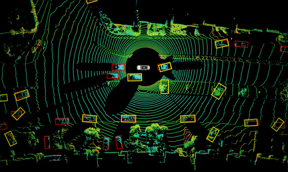
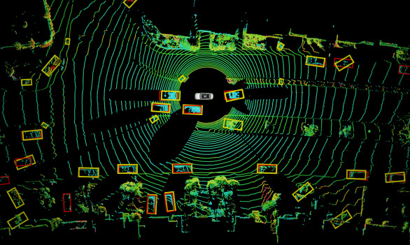
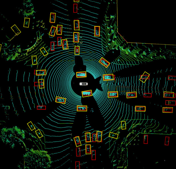
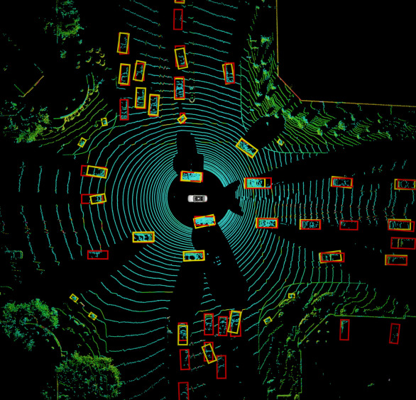
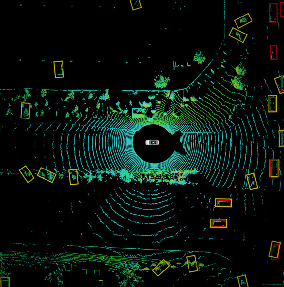
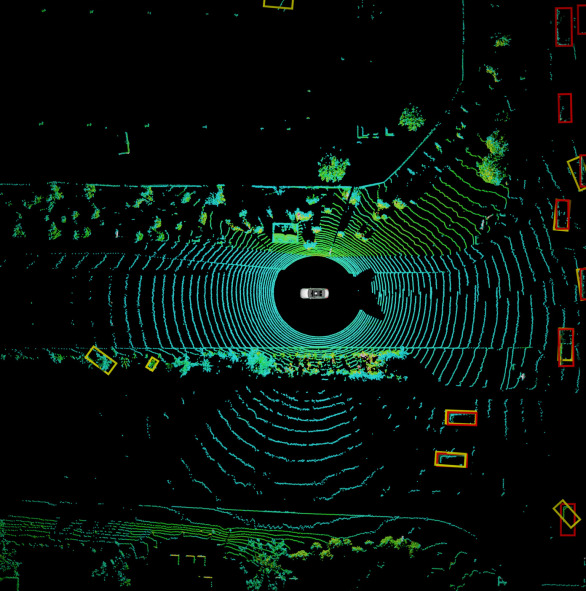
Figure 10: Qualitative Results on WOD. Red boxes are ground truth boxes, yellow are predictions. Left: OYSTER-CP Right: LISO-CP Both methods struggle to some extent with false positive detections, but Oyster much more so, despite using the higher confidence threshold. We attribute this to the fact that Oyster has noisier initial pseudo ground truth, which leads to wrong training signals.

Appendix 0.F Quantitative Results

In Table 7 and Table 6 we have more detailed metrics for WOD and nuScenes. Please note that models trained with our method get a high penalty on the Nuscenes Detection Score (NDS), because they cannot distinguish object classes and therefore score an Average Attribute Error of 1.0.

	method	AP$\uparrow$	NDS$\uparrow$	ATE$\downarrow$	AOE $\downarrow$	ASE$\downarrow$
GT	CP[30]	0.484	0.524	0.357	0.560	0.263
	TF[2]	0.627	0.614	0.287	0.501	0.207
Unsup.	DBSCAN[7]	0.008	0.109	0.987	3.120	0.962
	DBSCAN(SF)	0.003	0.106	1.186	2.623	0.952
	DBSCAN(GF)	0.000	0.000	1.000	1.0	1.0
	RSF[5]	0.019	0.183	0.774	1.003	0.507
Self Train	Oyster-CP[32]	0.091	0.215	0.784	1.514	0.521
	Oyster-TF[32]	0.093	0.233	0.708	1.564	0.448
	LISO-CP	0.109	0.224	0.750	1.062	0.409
	LISO-TF	0.134	0.270	0.628	0.938	0.408

Table 6: Full evaluation results on nuScenes  dataset: We compare LISO with two different network architectures (TF [2], CP [30]) against different baselines and also give supervised training results as reference (two top lines). Along the AP score we report the nuScenes detection score NDS, which is a combination of the AP score, average translation, orientation, scale, attribute error/score (ATE, AOE, ASE, AEE respectively). Note that nuScenes uses a minimum precision and recall threshold of 0.1, and since the recall of GT flow clustering is lower than 0.1, all results are clipped away. SF: lidar scene flow by SLIM, GF: ground truth lidar scene flow.

		Movable		Moving		Still		Vehicle		Pedestrian		Cyclist
		AP@0.4		AP@0.4		AP@0.4		AP@0.4		AP@0.4		AP@0.4
		BEV	3D	BEV	3D	BEV	3D	BEV	3D	BEV	3D	BEV	3D
GT	CP[30]	0.765	0.684	0.721	0.624	0.735	0.657	0.912	0.841	0.513	0.413	0.134	0.094
	TF[2]	0.746	0.723	0.714	0.668	0.733	0.710	0.918	0.899	0.457	0.429	0.216	0.187
Unsupervised	DBSCAN[7]	0.027	0.008	0.009	0.000	0.027	0.006	0.184	0.048	0.002	0.000	0.001	0.000
	DBSCAN(SF)	0.026	0.010	0.064	0.041	0.000	0.000	0.073	0.046	0.010	0.006	0.009	0.006
	DBSCAN(GF)	0.114	0.071	0.318	0.120	0.000	0.000	0.113	0.075	0.111	0.063	0.240	0.151
	RSF[5]	0.030	0.020	0.080	0.055	0.000	0.000	0.109	0.074	0.000	0.000	0.002	0.000
	SeMoLi [17] $\dagger$	-	0.195	-	0.575	-	-	-	-	-	-	-	-
	LISO-CP	0.292	0.211	0.272	0.204	0.208	0.140	0.607	0.440	0.029	0.009	0.010	0.004
Self Train	Oyster-CP[32]	0.217	0.084	0.151	0.062	0.176	0.056	0.562	0.204	0.000	0.000	0.000	0.000
	Oyster-TF[32]	0.121	0.015	0.051	0.007	0.098	0.010	0.475	0.058	0.000	0.000	0.000	0.000
	LISO-CP	0.380	0.308	0.350	0.296	0.322	|0.255	0.695	0.543	0.055	0.037	0.022	0.016
	LISO-TF	0.327	0.208	0.349	0.245	0.233	0.126	0.669	0.408	0.024	0.008	0.012	0.005

Table 7: Full evaluation results on WOD dataset: We evaluate using the protocol of [17, 13], using an area of whole 100$\mathrm{m}$$\times$40$\mathrm{m}$ BEV grid around the ego vehicle, considering objects that move faster than 1$\mathrm{m}\mathrm{/}\mathrm{s}$ to be moving (difficulty level L2). CP, TF: network architecture, in the first two lines trained supervised for comparison. $\dagger$: Results taken from [17]. SF: lidar scene flow by SLIM, GF: ground truth lidar scene flow.

References

- [1] Amini, M.R., Feofanov, V., Pauletto, L., Hadjadj, L., Devijver, E., Maximov, Y.: Self-training: A survey (2023)
- [2] Bai, X., Hu, Z., Zhu, X., Huang, Q., Chen, Y., Fu, H., Tai, C.: Transfusion: Robust lidar-camera fusion for 3d object detection with transformers. In: IEEE/CVF Conference on Computer Vision and Pattern Recognition, CVPR 2022, New Orleans, LA, USA, June 18-24, 2022. pp. 1080–1089. IEEE (2022). https://doi.org/10.1109/CVPR52688.2022.00116, https://doi.org/10.1109/CVPR52688.2022.00116
- [3] Baur, S.A., Emmerichs, D.J., Moosmann, F., Pinggera, P., Ommer, B., Geiger, A.: SLIM: self-supervised lidar scene flow and motion segmentation. In: 2021 IEEE/CVF International Conference on Computer Vision, ICCV 2021, Montreal, QC, Canada, October 10-17, 2021. pp. 13106–13116. IEEE (2021). https://doi.org/10.1109/ICCV48922.2021.01288, https://doi.org/10.1109/ICCV48922.2021.01288
- [4] Caesar, H., Bankiti, V., Lang, A.H., Vora, S., Liong, V.E., Xu, Q., Krishnan, A., Pan, Y., Baldan, G., Beijbom, O.: nuscenes: A multimodal dataset for autonomous driving. In: 2020 IEEE/CVF Conference on Computer Vision and Pattern Recognition, CVPR 2020, Seattle, WA, USA, June 13-19, 2020. pp. 11618–11628. IEEE (2020). https://doi.org/10.1109/CVPR42600.2020.01164, https://doi.org/10.1109/CVPR42600.2020.01164
- [5] Deng, D., Zakhor, A.: Rsf: Optimizing rigid scene flow from 3d point clouds without labels. In: Proceedings of the IEEE/CVF Winter Conference on Applications of Computer Vision (WACV). pp. 1277–1286 (January 2023)
- [6] Dewan, A., Caselitz, T., Tipaldi, G.D., Burgard, W.: Motion-based detection and tracking in 3d lidar scans. In: Kragic, D., Bicchi, A., Luca, A.D. (eds.) 2016 IEEE International Conference on Robotics and Automation, ICRA 2016, Stockholm, Sweden, May 16-21, 2016. pp. 4508–4513. IEEE (2016). https://doi.org/10.1109/ICRA.2016.7487649, https://doi.org/10.1109/ICRA.2016.7487649
- [7] Ester, M., Kriegel, H., Sander, J., Xu, X.: A density-based algorithm for discovering clusters in large spatial databases with noise. In: Simoudis, E., Han, J., Fayyad, U.M. (eds.) Proceedings of the Second International Conference on Knowledge Discovery and Data Mining (KDD-96), Portland, Oregon, USA. pp. 226–231. AAAI Press (1996), http://www.aaai.org/Library/KDD/1996/kdd96-037.php
- [8] Geiger, A., Lenz, P., Stiller, C., Urtasun, R.: Vision meets robotics: The KITTI dataset. Int. J. Robotics Res. 32(11), 1231–1237 (2013). https://doi.org/10.1177/0278364913491297, https://doi.org/10.1177/0278364913491297
- [9] Geiger, A., Lenz, P., Urtasun, R.: Are we ready for autonomous driving? the KITTI vision benchmark suite. In: 2012 IEEE Conference on Computer Vision and Pattern Recognition, Providence, RI, USA, June 16-21, 2012. pp. 3354–3361. IEEE Computer Society (2012). https://doi.org/10.1109/CVPR.2012.6248074, https://doi.org/10.1109/CVPR.2012.6248074
- [10] Harley, A.W., Zuo, Y., Wen, J., Mangal, A., Potdar, S., Chaudhry, R., Fragkiadaki, K.: Track, check, repeat: An EM approach to unsupervised tracking. In: IEEE Conference on Computer Vision and Pattern Recognition, CVPR 2021, virtual, June 19-25, 2021. pp. 16581–16591. Computer Vision Foundation / IEEE (2021). https://doi.org/10.1109/CVPR46437.2021.01631, https://openaccess.thecvf.com/content/CVPR2021/html/Harley_Track_Check_Repeat_An_EM_Approach_to_Unsupervised_Tracking_CVPR_2021_paper.html
- [11] Liang, Z., Zhang, Z., Zhang, M., Zhao, X., Pu, S.: Rangeioudet: Range image based real-time 3d object detector optimized by intersection over union. In: IEEE Conference on Computer Vision and Pattern Recognition, CVPR 2021, virtual, June 19-25, 2021. pp. 7140–7149. Computer Vision Foundation / IEEE (2021). https://doi.org/10.1109/CVPR46437.2021.00706, https://openaccess.thecvf.com/content/CVPR2021/html/Liang_RangeIoUDet_Range_Image_Based_Real-Time_3D_Object_Detector_Optimized_by_CVPR_2021_paper.html
- [12] Meyer, G.P., Laddha, A., Kee, E., Vallespi-Gonzalez, C., Wellington, C.K.: Lasernet: An efficient probabilistic 3d object detector for autonomous driving. In: IEEE Conference on Computer Vision and Pattern Recognition, CVPR 2019, Long Beach, CA, USA, June 16-20, 2019. pp. 12677–12686. Computer Vision Foundation / IEEE (2019). https://doi.org/10.1109/CVPR.2019.01296, http://openaccess.thecvf.com/content_CVPR_2019/html/Meyer_LaserNet_An_Efficient_Probabilistic_3D_Object_Detector_for_Autonomous_Driving_CVPR_2019_paper.html
- [13] Najibi, M., Ji, J., Zhou, Y., Qi, C.R., Yan, X., Ettinger, S., Anguelov, D.: Motion inspired unsupervised perception and prediction in autonomous driving. In: Avidan, S., Brostow, G.J., Cissé, M., Farinella, G.M., Hassner, T. (eds.) Computer Vision - ECCV 2022 - 17th European Conference, Tel Aviv, Israel, October 23-27, 2022, Proceedings, Part XXXVIII. Lecture Notes in Computer Science, vol. 13698, pp. 424–443. Springer (2022). https://doi.org/10.1007/978-3-031-19839-7_25, https://doi.org/10.1007/978-3-031-19839-7_25
- [14] Paszke, A., Gross, S., Massa, F., Lerer, A., Bradbury, J., Chanan, G., Killeen, T., Lin, Z., Gimelshein, N., Antiga, L., Desmaison, A., Köpf, A., Yang, E.Z., DeVito, Z., Raison, M., Tejani, A., Chilamkurthy, S., Steiner, B., Fang, L., Bai, J., Chintala, S.: Pytorch: An imperative style, high-performance deep learning library. In: Wallach, H.M., Larochelle, H., Beygelzimer, A., d’Alché-Buc, F., Fox, E.B., Garnett, R. (eds.) Advances in Neural Information Processing Systems 32: Annual Conference on Neural Information Processing Systems 2019, NeurIPS 2019, December 8-14, 2019, Vancouver, BC, Canada. pp. 8024–8035 (2019), https://proceedings.neurips.cc/paper/2019/hash/bdbca288fee7f92f2bfa9f7012727740-Abstract.html
- [15] Pedregosa, F., Varoquaux, G., Gramfort, A., Michel, V., Thirion, B., Grisel, O., Blondel, M., Prettenhofer, P., Weiss, R., Dubourg, V., Vanderplas, J., Passos, A., Cournapeau, D., Brucher, M., Perrot, M., Duchesnay, E.: Scikit-learn: Machine learning in Python. Journal of Machine Learning Research 12, 2825–2830 (2011)
- [16] Rist, C.B., Enzweiler, M., Gavrila, D.M.: Cross-sensor deep domain adaptation for lidar detection and segmentation. In: 2019 IEEE Intelligent Vehicles Symposium, IV 2019, Paris, France, June 9-12, 2019. pp. 1535–1542. IEEE (2019). https://doi.org/10.1109/IVS.2019.8814047, https://doi.org/10.1109/IVS.2019.8814047
- [17] Seidenschwarz, J., Ošep, A., Ferroni, F., Lucey, S., Leal-Taixé, L.: Semoli: What moves together belongs together (2024), https://arxiv.org/abs/2402.19463
- [18] Shen, Z., Liang, H., Lin, L., Wang, Z., Huang, W., Yu, J.: Fast ground segmentation for 3d lidar point cloud based on jump-convolution-process. Remote. Sens. 13(16), 3239 (2021). https://doi.org/10.3390/rs13163239, https://doi.org/10.3390/rs13163239
- [19] Shi, S., Wang, X., Li, H.: Pointrcnn: 3d object proposal generation and detection from point cloud. In: IEEE Conference on Computer Vision and Pattern Recognition, CVPR 2019, Long Beach, CA, USA, June 16-20, 2019. pp. 770–779. Computer Vision Foundation / IEEE (2019). https://doi.org/10.1109/CVPR.2019.00086, http://openaccess.thecvf.com/content_CVPR_2019/html/Shi_PointRCNN_3D_Object_Proposal_Generation_and_Detection_From_Point_Cloud_CVPR_2019_paper.html
- [20] Shin, S., Golodetz, S., Vankadari, M., Zhou, K., Markham, A., Trigoni, N.: Sample, crop, track: Self-supervised mobile 3d object detection for urban driving lidar. CoRR abs/2209.10471 (2022). https://doi.org/10.48550/arXiv.2209.10471, https://doi.org/10.48550/arXiv.2209.10471
- [21] Song, Z., Yang, B.: OGC: Unsupervised 3d object segmentation from rigid dynamics of point clouds. In: Oh, A.H., Agarwal, A., Belgrave, D., Cho, K. (eds.) Advances in Neural Information Processing Systems (2022), https://openreview.net/forum?id=ecNbEOOtqBU
- [22] Sun, P., Kretzschmar, H., Dotiwalla, X., Chouard, A., Patnaik, V., Tsui, P., Guo, J., Zhou, Y., Chai, Y., Caine, B., Vasudevan, V., Han, W., Ngiam, J., Zhao, H., Timofeev, A., Ettinger, S., Krivokon, M., Gao, A., Joshi, A., Zhang, Y., Shlens, J., Chen, Z., Anguelov, D.: Scalability in perception for autonomous driving: Waymo open dataset. In: 2020 IEEE/CVF Conference on Computer Vision and Pattern Recognition, CVPR 2020, Seattle, WA, USA, June 13-19, 2020. pp. 2443–2451. IEEE (2020). https://doi.org/10.1109/CVPR42600.2020.00252, https://doi.org/10.1109/CVPR42600.2020.00252
- [23] Sun, P., Wang, W., Chai, Y., Elsayed, G., Bewley, A., Zhang, X., Sminchisescu, C., Anguelov, D.: RSN: range sparse net for efficient, accurate lidar 3d object detection. In: IEEE Conference on Computer Vision and Pattern Recognition, CVPR 2021, virtual, June 19-25, 2021. pp. 5725–5734. Computer Vision Foundation / IEEE (2021). https://doi.org/10.1109/CVPR46437.2021.00567, https://openaccess.thecvf.com/content/CVPR2021/html/Sun_RSN_Range_Sparse_Net_for_Efficient_Accurate_LiDAR_3D_Object_CVPR_2021_paper.html
- [24] Träuble, B., Pauen, S., Poulin-Dubois, D.: Speed and direction changes induce the perception of animacy in 7-month-old infants. Frontiers in Psychology 5 (2014). https://doi.org/10.3389/fpsyg.2014.01141, https://www.frontiersin.org/articles/10.3389/fpsyg.2014.01141
- [25] Vizzo, I., Guadagnino, T., Mersch, B., Wiesmann, L., Behley, J., Stachniss, C.: KISS-ICP: in defense of point-to-point ICP - simple, accurate, and robust registration if done the right way. IEEE Robotics Autom. Lett. 8(2), 1029–1036 (2023). https://doi.org/10.1109/LRA.2023.3236571, https://doi.org/10.1109/LRA.2023.3236571
- [26] Wang, Y., Chen, Y., Zhang, Z.: 4d unsupervised object discovery. In: Koyejo, S., Mohamed, S., Agarwal, A., Belgrave, D., Cho, K., Oh, A. (eds.) Advances in Neural Information Processing Systems 35: Annual Conference on Neural Information Processing Systems 2022, NeurIPS 2022, New Orleans, LA, USA, November 28 - December 9, 2022 (2022), http://papers.nips.cc/paper_files/paper/2022/hash/e7407ab5e89c405d28ff6807ffec594a-Abstract-Conference.html
- [27] Wilson, B., Qi, W., Agarwal, T., Lambert, J., Singh, J., Khandelwal, S., Pan, B., Kumar, R., Hartnett, A., Pontes, J.K., Ramanan, D., Carr, P., Hays, J.: Argoverse 2: Next generation datasets for self-driving perception and forecasting. In: Proceedings of the Neural Information Processing Systems Track on Datasets and Benchmarks (NeurIPS Datasets and Benchmarks 2021) (2021)
- [28] Xu, J., Waslander, S.L.: Hypermodest: Self-supervised 3d object detection with confidence score filtering. CoRR abs/2304.14446 (2023). https://doi.org/10.48550/arXiv.2304.14446, https://doi.org/10.48550/arXiv.2304.14446
- [29] Yang, Z., Sun, Y., Liu, S., Jia, J.: 3dssd: Point-based 3d single stage object detector. In: 2020 IEEE/CVF Conference on Computer Vision and Pattern Recognition, CVPR 2020, Seattle, WA, USA, June 13-19, 2020. pp. 11037–11045. Computer Vision Foundation / IEEE (2020). https://doi.org/10.1109/CVPR42600.2020.01105, https://openaccess.thecvf.com/content_CVPR_2020/html/Yang_3DSSD_Point-Based_3D_Single_Stage_Object_Detector_CVPR_2020_paper.html
- [30] Yin, T., Zhou, X., Krähenbühl, P.: Center-based 3d object detection and tracking. In: IEEE Conference on Computer Vision and Pattern Recognition, CVPR 2021, virtual, June 19-25, 2021. pp. 11784–11793. Computer Vision Foundation / IEEE (2021). https://doi.org/10.1109/CVPR46437.2021.01161, https://openaccess.thecvf.com/content/CVPR2021/html/Yin_Center-Based_3D_Object_Detection_and_Tracking_CVPR_2021_paper.html
- [31] You, Y., Luo, K., Phoo, C.P., Chao, W., Sun, W., Hariharan, B., Campbell, M.E., Weinberger, K.Q.: Learning to detect mobile objects from lidar scans without labels. In: IEEE/CVF Conference on Computer Vision and Pattern Recognition, CVPR 2022, New Orleans, LA, USA, June 18-24, 2022. pp. 1120–1130. IEEE (2022). https://doi.org/10.1109/CVPR52688.2022.00120, https://doi.org/10.1109/CVPR52688.2022.00120
- [32] Zhang, L., Yang, A.J., Xiong, Y., Casas, S., Yang, B., Ren, M., Urtasun, R.: Towards unsupervised object detection from lidar point clouds. In: Proceedings of the IEEE/CVF Conference on Computer Vision and Pattern Recognition (CVPR). pp. 9317–9328 (June 2023)
- [33] Zhang, Y., Hu, Q., Xu, G., Ma, Y., Wan, J., Guo, Y.: Not all points are equal: Learning highly efficient point-based detectors for 3d lidar point clouds. In: IEEE/CVF Conference on Computer Vision and Pattern Recognition, CVPR 2022, New Orleans, LA, USA, June 18-24, 2022. pp. 18931–18940. IEEE (2022). https://doi.org/10.1109/CVPR52688.2022.01838, https://doi.org/10.1109/CVPR52688.2022.01838
- [34] Zhou, Y., Tuzel, O.: Voxelnet: End-to-end learning for point cloud based 3d object detection. In: 2018 IEEE Conference on Computer Vision and Pattern Recognition, CVPR 2018, Salt Lake City, UT, USA, June 18-22, 2018. pp. 4490–4499. IEEE Computer Society (2018). https://doi.org/10.1109/CVPR.2018.00472, http://openaccess.thecvf.com/content_cvpr_2018/html/Zhou_VoxelNet_End-to-End_Learning_CVPR_2018_paper.html