Multiset tomography: Optimizing quantum measurements by partitioning multisets of observables

Abstract

Quantum tomography approaches typically consider a set of observables which we wish to measure, design a measurement scheme which measures each of the observables and then repeats the measurements as many times as necessary. We show that instead of considering only the simple set of observables, one should consider a multiset of the observables taking into account the required repetitions, to minimize the number of measurements. This leads to a graph theoretic multicolouring problem. We show that multiset tomography offers at most quadratic improvement but it is achievable. Furthermore, despite the NP-hard optimal colouring problem, the multiset approach with greedy colouring algorithms already offers asymptotically quadratic improvement in test cases.

I Introduction

Quantum states generally cannot be measured without disturbing the state. Therefore, in order to estimate the expectation values of multiple observables, we might require a large number of copies of the same state. However, in order to reduce the quantum computational cost, we usually aim to minimize the number of state preparations. Some tomography methods approach this problem by restricting the states that can be considered to, e.g., Matrix Product States [1], or by restricting the observables that are measured to, e.g., $k$-local observables [2, 3]. Other notable methods include measuring in a random basis [4], or performing gentle measurements which disturb the original state as little as possible [5].

In our proposed method, no assumptions need to be made about the observables that we wish to measure, the state itself nor the types of operations that we are able to perform. However, we do make an implicit assumption that the number of observables grows at most polynomially with the system size. The reason for this is two-fold: With an exponential number of observables it is unlikely (although not impossible) that there exists an efficient measurement scheme at all. Furthermore, the exponential number of observables would inevitably mean an exponential classical overhead for our method.

We will show in this letter how partitioning the set of observables can be represented as a graph colouring problem. Similar reductions to graph colouring (or the equivalent problem of clique covers) have been considered especially in the context of Variational Quantum Eigensolvers in, e.g., [6, 7]. The multicolouring approach taken also in this paper was first considered in [8].

A common strategy for a tomography problem is to start by trying to find as optimal partition for the simple set of observables as possible and then repeat the measurements with that partition in order to achieve the targeted accuracy. However, we propose an alternative method taking into account the number of repetitions at the outset, as this provides a more complete and useful strategy. Consider the following simple example illustrating the main idea. Let a set of five observables be

$$S=\{Z_{1},Z_{2},X_{1}Z_{3},X_{1}X_{2},X_{2}X_{3}\},$$ (1)

where $Z_{i}$ denotes the Pauli Z operator on the $i$th qubit, i.e., $Z_{i}=I^{\otimes i-1}\otimes Z\otimes I^{\otimes n-i}$. Since we cannot measure non-commuting observables from the same shot, any partition of these observables must consist of at least three different sets, e.g.,

$$S=\{Z_{1},Z_{2}\}\cup\{X_{1}Z_{3},X_{1}X_{2}\}\cup\{X_{2}X_{3}\}.$$ (2)

However, if we assume that we want to measure each observable twice, instead of repeating with the same partition, we can overlap the partitions to come up with the following, more efficient measurement strategy

$$(Z_{1},Z_{2});(X_{1}Z_{3},X_{1}X_{2});(X_{2}X_{3},Z_{1});$$

$$(Z_{2},X_{1}Z_{3});(X_{1}X_{2},X_{2}X_{3}).$$ (3)

Therefore, instead of repeating the measurements with the partition of just one set of the observables, we should use a multiset containing as many instances of each observable as the number of times we need to measure them. These two different approaches are illustrated in Fig. 1. In this letter we will assume for pedagogical reasons that the multiplicity for each element is the same, but our method generalizes straightforwardly to the case of different multiplicities.

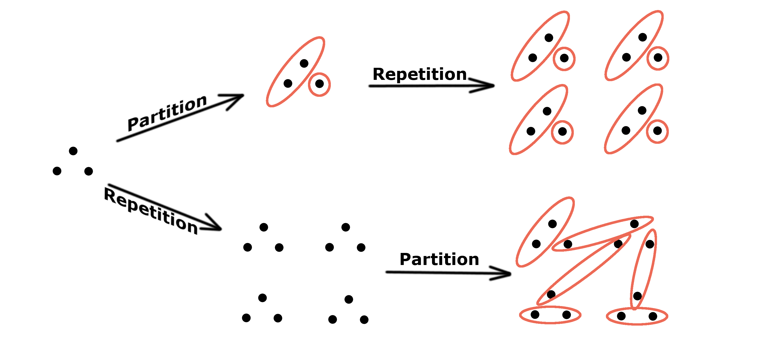
Figure 1: Instead of starting by partitioning the observables and then repeating measurements with the same partition, we can start by considering the number of needed repetitions and then construct the partition over the multiple instances of the same set.

We begin by establishing a bound on the improvement that can be achieved by partitioning the multiset instead of repeating $w$ times the measurements with the partition of the simple set. Let us denote by $d_{w}$ the number of sets required at minimum for partitioning $w$ multiples of the set of observables, which we will denote $S^{w}$.

Theorem 1.

Let $S$ be a set of observables and $S^{w}$ be a multiset where each element of $S$ is given a multiplicity of $w$. Also, let $d_{1}$ be the minimum number of sets required in partitioning $S$ into sets which can be measured from a single shot. Then, the number of sets $d_{w}$ required for partitioning the multiset $S^{w}$ is at least $\sqrt{wd_{1}}$.

Proof.

Each instance of an observable must belong to a different set in the partition and also the number of partitions cannot be less for the multiset than for the simple set. Therefore, we find that

$$d_{w}\geq\max(d_{1},w)\geq\sqrt{wd_{1}}.\qed$$ (4)

Since $wd_{1}$ would be the number of shots needed for repeating the partition of the simple set, the improvement cannot be better than quadratic. However, as we will see later, this quadratic improvement in asymptotic scaling is actually achievable in some scenarios.

II Multiset tomography

We begin by defining our task as follows. Let $S=\{O_{1},O_{2},\dots,O_{m}\}$ be a set of $m$ observables which we wish to measure. Furthermore, we define the following properties:

• A binary relation $O_{i}\sim O_{j}$ iff $O_{i}$ and $O_{j}$ can be measured in parallel.

• $\epsilon_{i}\in\mathbb{R}_{+}$ denoting the maximum error that we allow for each observable.

• Maximum probability of error $\delta\in[0,1]$. For simplicity, we will in this paper divide this error probability evenly with the observables so that each observable has its error probability bounded by $\delta/m$ ensuring that the total error probability is bounded by $\delta$.

With these constraints, we wish to minimize the number of shots, i.e., the number of copies of the original system that we need.

As a warm-up, we consider first a simplified problem ignoring repetitions, i.e., trying to measure each observable once without considering the accuracies and error probabilities. We will assume that the observables $O_{i}$ are chosen such that we know how to measure each of them on their own from a single shot. In DV (discrete variable) quantum tomography, these would usually be Pauli strings.

There may be constraints arising from the measurement protocol that are accounted for in the binary relation $\sim$ for the observables. E.g., based on the kind of operations we are able to perform, we might be able to measure all commuting observables in parallel, or only observables which commute on every single-qubit level. (We remark that $\sim$ defines a so-called independence relation, meaning that it is symmetric but not reflexive: $O_{i}\nsim O_{i}$. We can never perform multiple independent measurements of the same observable from the same shot: subsequent measurements of the same observable produce the same measurement result offering no new information. The relation is also not transitive.)

One method of representing such binary relations is with a graph. We can represent each observable as a vertex of a graph and draw an edge between two vertices if the corresponding observables cannot be measured in parallel. An example of such a graph is shown in Fig. 2 (a).

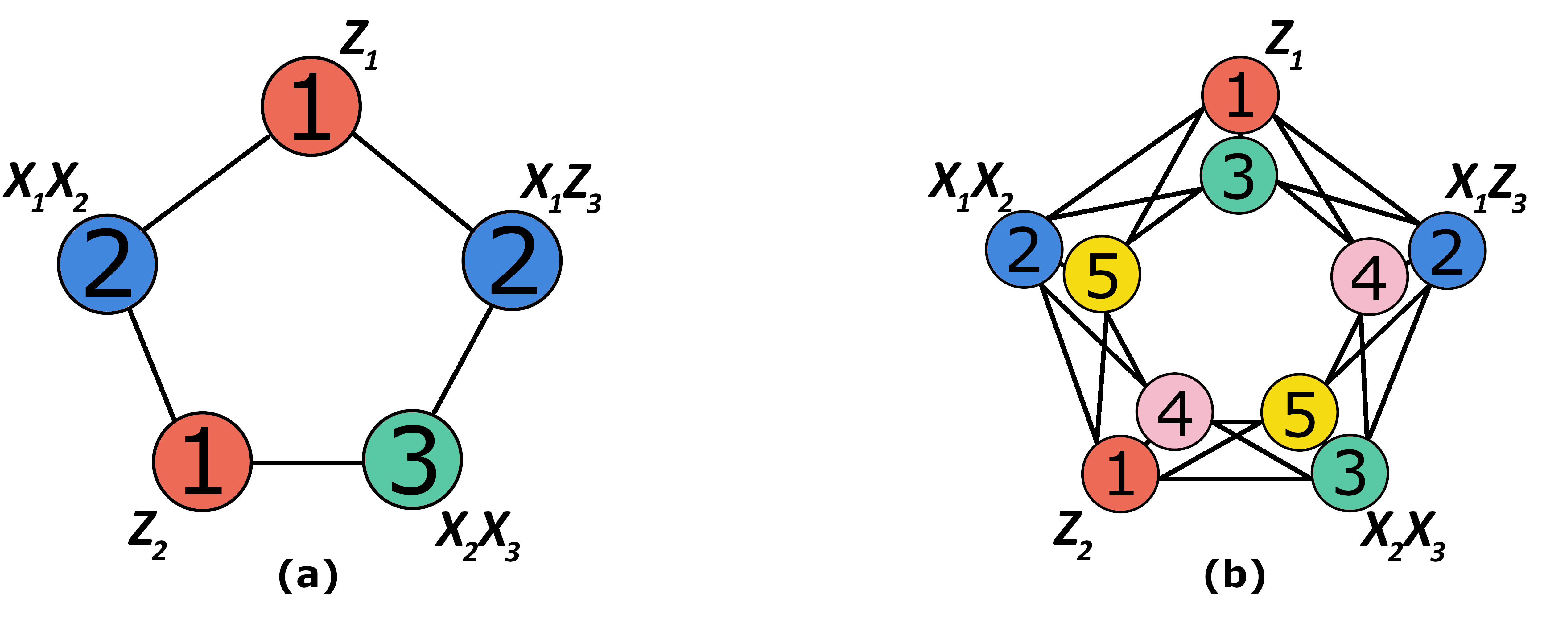
Figure 2: (a) The commutation relations of five observables illustrated as a graph. The numbers inside the vertices denote the colour labels for graph colouring. (b) Same five observables are given two colours each corresponding to different measurements. This time five colours/shots is enough to solve the problem.

Following these measurement restrictions, our aim would usually be to minimize the number of shots needed for measuring all of the observables. With the graph representation, this becomes a well-known mathematical problem known as graph colouring. In graph colouring, the aim is to colour each vertex of a graph with the constraint that any vertices sharing an edge cannot have the same colour. The minimum number of colours for a given graph is known as the chromatic number of the graph.

In our measurement setting, the vertices of the graph are the observables and each colour in the graph colouring would correspond to a different copy of the system. Thus the chromatic number of the observable graph would give the minimum number of shots needed to measure every observable once. In Fig. 2 (a) we have coloured the observable graph with three colours giving a measurement strategy with three shots.

However, solving the chromatic number of a graph and finding the corresponding colouring is an NP-hard problem so there are no known efficient, i.e., polynomial-time methods to solve them. Nonetheless, if we don’t need to find the optimal colouring, i.e., the most efficient measurement scheme, there are plenty of efficient graph colouring algorithms which can find some adequate solutions most of the time. As we discuss later, such colouring algorithms in multiset tomography are sufficient to provide advantage.

Next, we include the repetitions in our analysis. Measuring an observable only once gives randomly one of the possible eigenvalues. However, in order to characterize the original system with tomography, we are more likely interested in the expectation values of the observables. This means that we need to measure each observable multiple times.

Hoeffding’s inequality tells us that in order to achieve accuracy $\epsilon_{i}$ for the expectation value of observable $O_{i}$ with probability at least $1-\delta/m$, it is enough to measure that observable

$$w=\frac{2\ln\left(\frac{2m}{\delta}\right)}{\epsilon_{i}^{2}}$$ (5)

times, where we have assumed that $O_{i}$ has eigenvalues $\pm 1$ like Pauli strings. Therefore, one possible and perhaps the most common solution would be to repeat $w$ times the same measurement scheme that we came up with for the single measurements. However, this will not result in the most efficient measurement strategy.

The information about measurement repetitions can be included in the set partitioning approach by using multisets. A multiset is a generalization of a set, allowing also repetitions of elements. While the ordinary set listed each observable only once, with the multiset we can list them as many times as we need to measure them. Of course, this is merely one of the many possible ways to record the information about the repetitions. A benefit of the multiset approach becomes apparent when we compare partitioning the multiset as opposed to partitioning the simple set. Any partition of the simple set multiplied by the repetitions would still be a valid partition of the multiset as well, but the multiset also allows other partitions which are not apparent from the simple set perspective. The benefit is that the same strategies for finding those partitions work also for the multiset.

The binary relation between observables which we defined before still holds for the multiset and we can represent it as a graph as well. This is illustrated in Fig. 2 (b). The resulting graph replaces every vertex of the original graph with a clique of size equal to the number of repetitions. As with the simple set, colouring this graph is an equivalent problem to finding the measurement partition of the multiset. Alternatively, instead of replacing each vertex with a clique, we can also think of this as assigning each original vertex multiple colours. In that case, the problem is known in graph theory as multicolouring.

While partitioning the multiset can never perform worse than partitioning the simple set, Theorem 1 shows that the multiset approach cannot give more than quadratic improvement over the simple partition method. We will next show by an example that the quadratic improvement in asymptotic scaling can be achieved in some cases.

III Achievability of the quadratic improvement

We will consider the following problem: Let us have an $n$-qubit system for which we wish to measure every Pauli string of weight at most $k\geq 2$ (i.e., tensor products of Pauli matrices acting non-trivially on at most $k$ qubits). We will assume that we are able to perform only single-qubit operations. Even with the most naïve approaches we can measure at least $\lfloor n/k\rfloor$ of the observables from the same shot. With more elegant approaches, we can partition the set of observables into $\Theta(\log n)$ sets. We will show that this $\log n$ scaling is optimal, utilizing methods from [2].

Theorem 2.

Measuring (at least) once every Pauli string of weight at most $k\geq 2$ for an $n$-qubit system requires at least $\log_{2}n$ shots.

Proof.

Let us consider the problem of measuring either $Z_{i}X_{j}$ or $X_{i}Z_{j}$ for every $i,j\in\{1,\dots,n\}$. Since this set of observables is a (proper) subset of the original set of observables, this new problem clearly requires at most as many shots as the original problem. However, the minimum number of shots in this new problem is just the perfect hash family number PHFN$(n,2,2)$, which is known to be $\log_{2}n$ [9]. A more explicit proof is given in the supplemental material. ∎

The above construction is also the main principle behind the overlapping tomography method in [2]. However, this bound was for measuring each observable only once and we need to measure each observable $\Theta\left(\frac{\log(m/\delta)}{\epsilon^{2}}\right)$ times. Since $m=\Theta(n^{k})$, this means that we need to measure each observable $\Theta(\log n)$ times. Therefore, repeating the same measurements multiple times would result in at least $\Omega(\log^{2}n)$ shots. However, partitioning the multiset will result in only $\Theta(\log n)$ required shots.

Lemma 3.

Let us measure each qubit of an $n$-qubit system in a random Pauli basis ($X$, $Y$ or $Z$) for

$$d=\frac{2pw+\ln m}{p^{2}}$$ (6)

shots, where $p=3^{-k}$ and $k,w,m\in\mathbb{Z}_{+}$. Let $s$ denote the number of times we have measured a given $k$-weight Pauli string. Then, the probability that $s\leq w$ is

$$P(s\leq w)<\frac{1}{m}.$$ (7)

Proof.

The probability that we measure the given Pauli string from a single shot is $p=3^{-k}$. Hoeffding’s inequality tells us (see supplemental material Corollary S2.3 where, now, the random variable $X_{i}=1$ if we have measured the Pauli string from the $i$th shot and $X_{i}=0$ if we have not) that the probability of measuring the Pauli string at most $w$ times is

$$P(s\leq w) \leq \exp\left[-2\left(p-\frac{w}{d}\right)^{2}d\right]$$ (8)

$$= \exp\left[-2\frac{(pw+\ln m)^{2}}{2pw+\ln m}\right]$$

$$< \exp[-\ln m]=\frac{1}{m}.$$

∎

Theorem 4.

Let $S^{w}$ be a multiset consisting of every $k$-weight Pauli string of an $n$-qubit system each with multiplicity $w=a\ln n$, where $n\geq 3$ and $a\in\mathbb{R}_{+}$. There exists a partition of this multiset into

$$d=2(3^{k}a+3^{2k}k)\ln n$$ (9)

sets where any two elements of a single set commute on a single-qubit level.

Proof.

Using Lemma 3 with $w=a\ln n$ and $m=\binom{n}{k}3^{k}$, we find that with

$$d=2\times 3^{k}a\ln n+3^{2k}\ln\left[\binom{n}{k}3^{k}\right]\leq 2(3^{k}a+3^{2k}k)\ln n$$ (10)

shots we have measured any given $k$-weight Pauli string at least $a\ln n$ times with probability greater than $1-1/m$. Therefore, we have measured all $m$ of them at least $a\ln n$ times with probability greater than 0. This non-zero probability proves that there must exist a set of $N$ measurements which measures every $k$-weight Pauli string at least $a\ln n$ times and this set of measurements gives us the desired partition. ∎

Theorem 4 shows that by partitioning the multiset of observables, the required number of shots grows asymptotically only as $\Theta(\log n)$. In order to compare with the earlier lower bound for simple set partition, we should still sum eq. 9 over $k$ since the simple set bound was for Pauli observables with weight up to $k$. However, this does not affect the asymptotic scaling (as a function of $n$) so it gives a quadratic improvement to the scaling of $\Omega(\log^{2}n)$ shots needed for partitioning the simple set and then repeating those measurements for the required number of times. We will next apply the multiset tomography method in a concrete example, and demonstrate that a quadratic improvement can also be achieved in practice.

IV Example

We begin by addressing the important question for practical applications: the computational cost of finding the partitions. As mentioned before, even with the best known methods, the time required for finding the optimal colouring of a graph scales exponentially with the graph size. Since the multiset approach also expands the size of the graph significantly, attempting to find the optimal solution would be futile. However, two simple tricks allow us to benefit from the multiset approach. First of all, we don’t need to find the optimal solution, just some acceptably good solution. In our test cases the linear-time greedy algorithm (GA) has proven to work extremely well. GA takes the set of vertices in random order and then gives each vertex the lowest possible colour allowed by the already coloured neighbours of that vertex.

Another way to limit the computational time is by limiting the number of repetitions we consider in the multiset. While the number of repetitions of measurements for each observable can be quite large, we can construct the multiset with just a fraction of those repetitions and then repeat the partition of that multiset as many times as needed. Even a small number of repeated instances of observables in the multiset can decrease the required number of shots quite significantly.

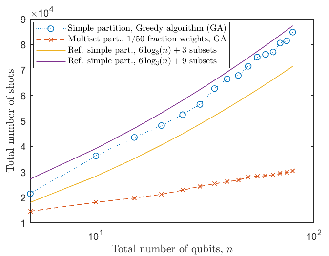
Figure 3: Greedy algorithm’s (GA) performance for both the simple set partition and multiset partition compared to a known deterministic partition method [3]. GA for the simple partition (dotted line with circles), while non-deterministic, seems to perform roughly the same as the reference method (solid lines). However, GA for the multiset partition (dashed line with x’s) performs much better even with just 1/50 of the actual measurement repetitions considered in the multiset.

As an example to show that the GA performs satisfactorily well, and that it is unnecessary to include the full number of measurement repetitions in the graph colouring, in Fig. 3 we show some experimental results for the previously considered problem of measuring $k$-local Pauli observables for the $k=2$ case with $\epsilon=\delta=0.1$. The solid lines represent some reference values for the simple partition case. More specifically, the lower solid line assumes a partition of the simple set with $6\log_{3}n+3$ subsets while the upper solid line assumes a partition with $6\log_{3}n+9$ subsets. These values are based on [3], where it is shown that for this specific problem there exists a partition with $6\lceil\log_{3}n\rceil+3$ subsets.

Our experimental GA line for simple partition (dotted line with circles) remains within these two values, so it performs roughly the same. For the multiset partition we have limited the number of colours for each observable to 1/50 of the actual number of measurement repetitions (and then repeated that solution 50 times). With the logarithmic x-axis for the number of qubits, this multiset partition line (dashed line with x’s) remains roughly linear and performs significantly better than the simple set partition lines.

V Summary and discussion

It is easy to see that multiset tomography should always perform at least as well as any other method, especially if we compare it to a simple partition of the observables. This is because the multiset partition tries to find the optimal out of all possible mesurement strategies. As shown, the improvement over the simple partition can never be more than quadratic, but there exist problems where the asymptotic scaling achieves that quadratic improvement. We have also demonstrated methods for reducing the (classical) computational cost of partitioning the multiset by using heuristic algorithms and using only a fraction of the observable repetitions in the multiset.

We used random measurements to show the existence of a quadratically improved solution for our example problem. Therefore, it should come as no surprise that the random measurements also achieve this quadratic improvement in asymptotic scaling for this particular problem. Indeed, the methods in [4] can be used to give an upper bound of

$$d=\frac{68\times 3^{k}\ln\left(\frac{2m}{\delta}\right)}{\epsilon^{2}}$$ (11)

shots, which we have slightly improved to

$$d=\frac{8\times 3^{k-1}\ln\left(\frac{2m}{\delta}\right)}{\epsilon^{2}}$$ (12)

for random measurements (see supplemental material). However, while random measurements would be efficient for that particular problem, they would not work for more general problems unlike our proposed method. In the example case, we considered only Pauli observables acting nontrivially on a small number of qubits (i.e., relatively small $k$) which is particularly suited for random measurements but as soon as the observables involve a larger number of qubits, the probability of measuring them with random measurements decreases exponentially. The multiset partitioning method, on the other hand, does not have this same flaw as it treats all observables equally.

A further advantage is that this easily generalises to problems where the needed measurement repetitions vary between observables. While most methods would end up sharing the maximum value of measurements for all observables, there is no reason why the multiplicities of each observable should be equal in the multiset. Instead, we can scale the multiplicities for each observable proportional to the number of times they need to be measured.

It would also be interesting to study whether our multiset partition approach would have applications beyond the quantum information field. As the method should be suitable to any problem where a mix of independent and non-independent operations are performed repeatedly, it could perhaps also be used in, e.g., manufacturing.

References

- Lanyon et al. [2017] B. P. Lanyon, C. Maier, M. Holzäpfel, T. Baumgratz, C. Hempel, P. Jurcevic, I. Dhand, A. S. Buyskikh, A. J. Daley, M. Cramer, M. B. Plenio, R. Blatt, and C. F. Roos, Nature Physics 13, 1158–1162 (2017).
- Cotler and Wilczek [2020] J. Cotler and F. Wilczek, Phys. Rev. Lett. 124, 100401 (2020).
- García-Pérez et al. [2020] G. García-Pérez, M. A. C. Rossi, B. Sokolov, E.-M. Borrelli, and S. Maniscalco, Phys. Rev. Res. 2, 023393 (2020).
- Huang et al. [2020] H.-Y. Huang, R. Kueng, and J. Preskill, Nat. Phys. 16, 1050 (2020).
- Aaronson and Rothblum [2019] S. Aaronson and G. N. Rothblum, in Proceedings of the 51st Annual ACM SIGACT Symposium on Theory of Computing, STOC 2019 (Association for Computing Machinery, New York, NY, USA, 2019) p. 322–333.
- Verteletskyi et al. [2020] V. Verteletskyi, T.-C. Yen, and A. F. Izmaylov, The Journal of Chemical Physics 152, 10.1063/1.5141458 (2020).
- Huggins et al. [2021] W. J. Huggins, J. R. McClean, N. C. Rubin, Z. Jiang, N. Wiebe, K. B. Whaley, and R. Babbush, npj Quantum Information 7, 10.1038/s41534-020-00341-7 (2021).
- Veltheim [2022] O. Veltheim, Quantum State Tomography with Observable Commutation Graphs, Master’s thesis, University of Helsinki (2022).
- II and Colbourn [2007] R. A. W. II and C. J. Colbourn, Journal of Mathematical Cryptology 1, 125 (2007).