NLO+NLL’ accurate predictions for three-jet event shapes in hadronic Higgs decays

Abstract

We present resummed predictions at next-to-leading logarithmic accuracy matched to the exact next-to-leading order results for a set of classical event-shape observables in hadronic Higgs decays, i.e., for the channels $H\to gg$ and $H\to b\bar{b}$. We furthermore consider soft-drop grooming of the hadronic final states and derive corresponding NLO +$\text{NLL}^{\prime}$ predictions for the groomed thrust observable. Differences in the QCD radiation pattern of gluon- and quark-initiated final states are imprinted in the event-shape distributions, offering separation power for the two decay channels. In particular, we show that ungroomed event shapes in $H\to gg$ decays develop a considerably harder spectrum than in $H\to b\bar{b}$ decays. We highlight that soft-drop grooming can substantially alter this behaviour, unless rather inclusive grooming parameters are chosen.

1 Introduction

A new high-energy lepton collider, such as the FCC-ee [1, 2], the CEPC [3], or the ILC [4], operated in the Higgs-factory mode presents a key scenario for future particle-physics collider experiments. The primary goal of these facilities lies in the precise determination of the properties of the Higgs-boson particle, recently discovered by the ATLAS and CMS experiments at the LHC [5, 6]. This includes detailed measurements of its decay width and branching fractions, and hence its couplings, as well as differential distributions of its decay final states at unprecedented precision.

The dominant production mode of Higgs bosons at leptonic Higgs factories proceeds via the Higgs-strahlungs process, i.e., in association with a $Z$-boson, through $e^{+}e^{-}\to ZH$. The absence of hadronic initial-state radiation in lepton–lepton collisions facilitates the investigation of hadronic Higgs-boson decays that are inaccessible at hadron colliders such as the LHC. This is in particular the case for the Higgs decaying into gluons. To this end, leptonic decays of the gauge boson are considered, leading to the experimental signature $e^{+}e^{-}\to l^{+}l^{-}+X_{\text{QCD}}$, with $X_{\text{QCD}}$ the hadronic final state originating from the Higgs-boson decay, e.g., through $H\to q\bar{q}$ and $H\to gg$. For the cases $H\to b\bar{b}$ and $H\to c\bar{c}$, displaced vertices emerging from weak decays of bottom- and charm-flavoured hadrons can be instrumented  [7, 8, 9, 10], providing means to disentangle these from the gluon decay mode. However, also differences in the QCD radiation pattern for quark- and gluon-initiated final states offer discriminatory power [11, 12, 13, 14, 15, 16]. A particular class of observables sensitive to these radiative corrections are event-shape variables, that probe the geometric properties of the hadronic final state. Event-shape observables played a prominent role in the analysis of QCD final states produced in electron–positron annihilation at LEP [17, 18, 19, 20, 21]. In particular, they have been, and still are, instrumental for precision extractions of the strong coupling $\alpha_{\text{s}}$ [22]. These analyses pertaining to three-jet-like event shapes in hadronic $Z$-boson and off-shell photon decays are facilitated by precision calculations, including the evaluation of next-to-next-to-leading order (NNLO) corrections in the strong coupling [23, 24, 25, 26, 27, 28, 29, 30] and the resummation of logarithmically enhanced terms [31, 32, 33, 34, 35, 36, 37, 38]. Recently, also power corrections related to hadronisation effects have been taken into account [39, 40, 41, 42, 43]. Furthermore, measurements of event shapes provide a crucial test-bed for Monte Carlo event generators, based on parton-shower simulations and phenomenological models for hadronisation [44, 45]. It is worth noting, that QCD final states produced at LEP are dominated by the hadronic decays $\gamma^{*}/Z\to q\bar{q}$, such that gluon-initiated jets are much less constrained. This motivates dedicated studies of event shapes in hadronic Higgs-boson decays, both at fixed order in perturbation theory and for resummation calculations.

Beyond the direct comparison to existing or future experimental data, theoretical predictions for Higgs-boson decays to quarks and in particular gluons are used as proxies in jet-flavour tagging studies, in particular to investigate related theoretical and modelling uncertainties. Given that a theoretically clean definition of a quark/gluon jet is in itself a complicated research topic [46, 47, 48, 49, 50, 51, 52, 53], it is often unclear where to start if one seeks for a detailed understanding of the systematics involved. A common solution to study light-quark and gluon tagging, for example in the studies performed in [54, 55, 56, 57], is to take Higgs-boson decays to gluons as a clean probe of gluon-induced jets, and the decay of a singlet to quarks as the corresponding counterpart. A detailed understanding of the involved perturbative inputs, provided for a large variety of relevant observables, is a crucial element for future studies in this area.

First resummed predictions for thrust in $H\to gg$ decays at $\text{NNLL}^{\prime}$ accuracy have been presented in [56]. $\text{NNLL}^{\prime}$ results for the class of angularity variables have recently been derived in  [58, 59]. A few approaches that combine a fixed-order calculation matched to NNLL resummation with full event-generation frameworks have been derived for hadronic Higgs decays. The Geneva collaboration compiled results based on the NNLO fixed-order calculation for two-body decays with NNLL 2-jettiness resummation for both Higgs decay channels [60]. Similarly, the approach presented in [61] utilises NNLL resummation of the thrust observable to combine two-body decays at NNLO with parton showers. Within the MiNLO scheme, a NNLO calculation of the $H\to b\bar{b}$ decay is embedded into a full event-simulation framework via NNLL resummation of the three-jet resolution variable in the Cambridge–Aachen algorithm [62].

We here consider the matching of exact next-to-leading order QCD predictions for six classic three-jet event shapes recently presented in Ref. [63] with resummed predictions at next-to-leading logarithmic accuracy, evaluated using the implementation of the C AESAR resummation formalism [64] in the S HERPA event generator framework [65]. We thereby consider in particular thrust, $C$-parameter, heavy-hemisphere mass, total and wide jet broadening, and the Durham three-jet resolution variable $y^{\mathrm{D}}_{23}$. Furthermore, we here derive and present predictions for soft-drop thrust [66] for three values of the soft-drop angular parameter $\beta$, namely $\beta=0,1,2$.

Our paper is organised as follows: In Sec. 2 we describe our theoretical framework, providing details about the fixed-order and resummed computations. Furthermore, we introduce the considered event-shape observables. In Sec. 3 we cross-validate our calculations by considering the soft limit for the fixed-order predictions and the expansions of the resummation to ${\cal{O}}(\alpha_{\text{s}})$ and ${\cal{O}}(\alpha_{\text{s}}^{2})$. Our final matched predictions with $\text{NLO}+\text{NLL}^{\prime}$ accuracy are presented in Sec. 4. Finally, we give our conclusions and a brief outlook on future research avenues in Sec. 5.

2 Theoretical framework

The computation of three-jet like event-shape observables related to hadronic Higgs decays is performed in an effective field theory framework, where two distinct classes of processes arising through the two-parton decay modes $H\to gg$ and $H\to b\bar{b}$ are considered. In the former case, the Higgs boson couples to gluons via a heavy-quark loop which decouples in the limit of an infinitely-large top-quark mass. More precisely, we compute differential decay rates in the limit of vanishing light-quark masses, while keeping a non-vanishing Yukawa coupling $y_{b}$ only for the bottom quark and an infinitely large top-quark mass. As a consequence, the hadronic decay modes of the Higgs boson can be divided into two categories at parton-level: In the first category, the Higgs decays into a bottom–anti-bottom pair and is related to the non-vanishing Yukawa coupling $y_{b}$. In the second category, related to the decay of the Higgs boson to gluons, observables are computed in an effective theory approach in which the Higgs boson couples directly to gluons through an effective Higgs-gluon-gluon vertex. The latter vertex originates from a closed top-quark loop, considered in the infinite top-mass limit [67, 68, 69]. Both Higgs decay modes to two partons are depicted in Fig. 1, where the effective $Hgg$ vertex is represented as a crossed dot.

The framework used here can be formulated in terms of an effective Lagrangian as presented in [63]:

$$\mathcal{L}_{\mathrm{Higgs}}=-\frac{\lambda(m_{t},\mu_{\text{R}})}{4}HG_{\mu\nu}^{a}G^{a,\mu\nu}+\frac{y_{b}(\mu_{\text{R}})}{\sqrt{2}}H\bar{\psi}_{b}\psi_{b}\,.$$ (1)

In this context, the effective $Hgg$ coupling is given in terms of the Wilson coefficient $C(m_{t},\mu_{\text{R}})$ by

$$\lambda(m_{t},\mu_{\text{R}})=-\frac{\alpha_{\text{s}}(\mu_{\text{R}})C(m_{t},\mu_{\text{R}})}{3\uppi}\frac{4\uppi\alpha}{2m_{\mathrm{W}}\sin\theta_{\mathrm{W}}}\,,$$ (2)

and the $Hb\bar{b}$ Yukawa coupling reads

$$y_{b}(\mu_{\text{R}})=\overline{m}_{b}(\mu_{\text{R}})\frac{4\uppi\alpha}{\sqrt{2}m_{\mathrm{W}}\sin\theta_{\mathrm{W}}}\,.$$ (3)

Here, $\alpha$ denotes the electromagnetic coupling and $\theta_{\mathrm{W}}$ is the Weinberg angle. Both $\lambda$ and $y_{b}$ are subject to renormalisation, which we perform at scale $\mu_{\text{R}}$ in the $\overline{\text{MS}}$ scheme using $N_{\mathrm{F}}=5$. The top-quark Wilson coefficient is evaluated at first order in $\alpha_{\text{s}}$ using the results of [70, 71, 72, 73, 74, 75, 76].

It is important to stress that the terms in Eq. (1) do not interfere under the assumption of kinematically massless quarks. In particular, they do not mix under renormalisation [12]. This allows us to define two separate Higgs-decay categories, as mentioned above, and to compute higher-order corrections independently for each. All partonic contributions with three hard final-state partons at Born level that are needed for the fixed-order parton-level calculations used in this paper have been presented up to $\mathcal{O}(\alpha_{\text{s}}^{2})$ in [63].

In what follows, we will describe the calculational tools and setups used to derive our fixed-order and resummed predictions for a set of widely considered event-shape observables obtained in both Higgs-decay categories. For the case of the thrust variable [77, 78] we furthermore consider its soft-drop groomed variant [66], where the hadronic final state prior to the observable evaluation is subjected to soft-drop grooming [79].

Figure 1: Higgs to two-parton contributions to the hadronic Higgs-boson decays: $H\to b\bar{b}$ proportional to the Yukawa coupling $y_{b}$, and $H\to gg$ mediated through an effective coupling.

NLO calculation

For an infrared and collinear safe event-shape observable $V$, a function of the hadronic final state momenta, that yields the observable value $v$, the differential hadronic-decay width can be written up to NLO in the strong coupling $\alpha_{\text{s}}$ as

$$\frac{1}{\Gamma_{2j}}\frac{\mathrm{d}\Gamma}{\mathrm{d}v}=\frac{\alpha_{\text{s}}(\mu_{\text{R}})}{2\uppi}\frac{\mathrm{d}A}{\mathrm{d}v}+\left(\frac{\alpha_{\text{s}}(\mu_{\text{R}})}{2\uppi}\right)^{2}\frac{\mathrm{d}B}{\mathrm{d}v}\,,$$ (4)

with the leading-order (LO) coefficient $A$ and the next-to-leading order (NLO) coefficient $B$. In this context, $\Gamma_{2j}$ defines the inclusive partial decay width in the respective decay channel,

$$\Gamma_{b\bar{b}}(\mu_{\text{R}})=\frac{y_{b}^{2}(\mu_{\text{R}})m_{H}N_{\text{C}}}{8\uppi}\,,\quad\Gamma_{gg}(\mu_{\text{R}})=\frac{\alpha_{\text{s}}^{2}(\mu_{\text{R}})G_{\mathrm{F}}m_{H}^{3}}{36\uppi^{3}\sqrt{2}}\,,$$ (5)

where $N_{\text{C}}=3$ is the number of colours, $G_{\mathrm{F}}=4\uppi\alpha/(4\sqrt{2}m_{\mathrm{W}}^{2}\sin^{2}\theta_{\mathrm{W}})$ denotes the Fermi constant and $m_{H}$ stands for the Higgs-boson mass.

We calculate the perturbative coefficients $A$ and $B$ using the E ERAD 3 parton-level event generation framework. Originally developed for NNLO calculations of event shapes [23, 24] and jet distributions [80] for $\gamma^{*}/Z$-decays related to $e^{+}e^{-}\to 3j$, E ERAD 3 has recently been extended to include hadronic Higgs decays to three [63, 81] and four jets [82] in the $H\to b\bar{b}$ and $H\to gg$ channels at NLO level. As alluded to above, the computation of three jet-like Higgs event-shapes involving the hadronic Higgs decays to three hard partons at the Born-level are performed assuming an effective Lagrangian obtained under the assumptions of an infinitely heavy top-quark, i.e., $m_{t}\to\infty$, and massless light quarks, $m_{q}\equiv 0$, where only the $b$-quark has a non-vanishing Yukawa coupling $y_{b}>0$.

Infrared singularities are regulated using the antenna-subtraction scheme [83, 84, 85] to construct real and virtual subtraction terms. All tree-level and virtual matrix elements are implemented in fully analytic form, assuring stable numerical predictions even for infrared kinematics. All event-shape distributions are calculated above a cut of $v_{\mathrm{cut}}$, so that $v>v_{\mathrm{cut}}$. For all observables except the three-jet resolution scale, a cut of $v_{\mathrm{cut}}=10^{-5}$ is chosen; for the three-jet resolution variable, the cut is lowered to $v_{\mathrm{cut}}=10^{-10}$. For the renormalisation scale entering the calculation we use as central value $\mu_{\text{R}}=m_{H}$. We employ one- and two-loop running for the strong coupling $\alpha_{\text{s}}$ for the LO and NLO calculations, respectively. As input at scale $m_{Z}$ we use $\alpha_{\text{s}}(m_{Z})=0.118$.

NLL resummation

We derive all-orders results for the event-shape observables at next-to-leading logarithmic (NLL) accuracy using the implementation of the C AESAR formalism [64] in the S HERPA event-generator framework [86, 87], first presented in [65]. Within the C AESAR approach one considers infrared- and collinear-safe (IRC-safe) observables $V$ that scale for the emission of a soft-gluon of relative transverse momentum $k_{t}^{(l)}$, rapidity $\eta^{(l)}$, and azimuthal angle $\phi^{(l)}$ with respect to leg $l$ of the Born-level process as

$$V(k)=\left(\frac{k_{t}^{\left(l\right)}}{\mu_{Q}}\right)^{a}e^{-b_{l}\eta^{\left(l\right)}}d_{l}\left(\mu_{Q}\right)g_{l}\left(\phi^{(l)}\right)\,.$$ (6)

For the global event-shape observables considered here and a specific partonic channel $\delta$, the NLL accurate all-order cumulative cross section for observable values up to $v$, with $L=-\ln(v)$, can be written as

$$\Gamma_{\text{NLL}}(v)=\int\mathop{\mathrm{d}\mathcal{B}}\frac{\mathop{\mathrm{d}\Gamma_{2j}}}{\mathop{\mathrm{d}\mathcal{B}}}\exp\left[-\sum_{l\in\mathcal{B}}R_{l}(L)\right]\mathcal{F}(L)\,.$$ (7)

Here, $\mathop{\mathrm{d}\Gamma_{2j}}/\mathop{\mathrm{d}\mathcal{B}}$ denotes the Born-level cross section; $R_{l}$ the collinear radiators; and $\mathcal{F}$ is the multiple-emission function.

In Ref. [88] the C AESAR formalism, and in particular the radiator functions $R_{l}$, and the corresponding implementation in S HERPA were extended to include the phase-space constraints given by soft-drop grooming with general parameters $z_{\text{cut}}$ and $\beta$ [79]. The framework has recently been used to obtain resummed predictions for soft-drop thrust [66] and multijet resolution scales [89] in electron–positron annihilation, as well as $\text{NLO}+\text{NLL}^{\prime}$ predictions for soft-drop groomed hadronic event shapes [88], jet angularities in dijet and $Z$+jet production at the LHC [48, 90, 91] and, lately, for plain and groomed 1-jettiness in deep inelastic scattering [92].

$\text{NLO}+\text{NLL}^{\prime}$ matching

We here consider combining the resummation to NLL with exact NLO results for three-jet event shapes using a multiplicative matching scheme, thereby aiming for $\text{NLO}+\text{NLL}^{\prime}$ accuracy. Starting from Eq. (4), we can introduce the decay width for events with observable values up to $v$,

$$\Gamma(v)\equiv\int_{0}^{v}\mathrm{d}v\frac{\mathrm{d}\Gamma_{2j}}{\mathrm{d}v}=\Gamma_{2j}\left(1+\frac{\alpha_{\text{s}}(\mu_{\text{R}})}{2\uppi}A(v)+\left(\frac{\alpha_{\text{s}}(\mu_{\text{R}})}{2\uppi}\right)^{2}B(v)\right)\,,$$ (8)

where $A(v)$ is normalised so that the full integral over $v$, i.e., $A(v_{\text{max}})$, reproduces the NLO correction to $\Gamma_{2j}$. Note that this does not change the functional form of Eq. (4).

The logarithmic structure of $\Gamma(v)$ at order $\alpha_{\text{s}}^{n}$ contains up to $2n$ powers of the logarithm $L=-\ln(v)$. Hence, we separate each of $A(v)$, $B(v)$ into terms $A_{i}$, $B_{j}$ containing $i\leq 2$ and $j\leq 4$ powers of $L$, and a finite remainder that vanishes in the $v\to 0$ limit. Explicitly, we write

$$A(v) =L^{2}A_{2}+LA_{1}+A_{0}+A_{\text{finite}}(v)\,,$$ (9)

$$B(v) =L^{4}B_{4}+L^{3}B_{3}+L^{2}(B_{2}+A_{0}A_{2})+LB_{1}+B_{0}+B_{\text{finite}}(v)\,.$$ (10)

We have chosen to make it explicit in our notation that the coefficient of $L^{2}$ in $B(v)$ receives contributions that can be constructed from the ones present in $A(v)$ as well as generic NLO corrections $B_{2}$. In principle, the same is true for $B_{1}$, $B_{0}$, and $B_{\text{finite}}$, which we suppress since these coefficients are not completely restored at NLL^′ accuracy anyway. Comparing to other conventions used in the literature, for example [93], we can identify the constants and finite remainders with

$$A_{0}=\mathcal{C}_{1}\,,\;\; A_{\text{finite}}(v)=\mathcal{D}_{1}(v)\,,$$ (11)

$$B_{0}=\mathcal{C}_{2}\,,\;\; B_{\text{finite}}(v)=\mathcal{D}_{2}(v)\,.$$ (12)

For observables satisfying the conditions for automated NLL resummation outlined in [64], in particular recursive IRC safety, the NLL resummed cross section takes the well-known form

$$\Gamma_{\text{NLL}}(v)=\Gamma_{2j}\exp(Lg_{1}(\alpha_{\text{s}}L)+g_{2}(\alpha_{\text{s}}L))\,.$$ (13)

When expanding the resummed all-orders cross section to second order in $\alpha_{\text{s}}$, and sorting according to logarithmic enhancement in the same terms as in Eqs. (9), (10) we obtain

$$\Gamma_{\text{NLL}}(v)\sim\Gamma_{2j}\left(1+\frac{\alpha_{\text{s}}(\mu_{\text{R}})}{2\uppi}A_{\text{NLL}}+\left(\frac{\alpha_{\text{s}}(\mu_{\text{R}})}{2\uppi}\right)^{2}B_{\text{NLL}}+\mathcal{O}(\alpha_{\text{s}}^{3})\right)\,,$$ (14)

where

$$A_{\text{NLL}}(v) = L^{2}A_{2}+LA_{1}\,,$$ (15)

$$B_{\text{NLL}}(v) = L^{4}B_{4}+L^{3}B_{3}+L^{2}B_{2}\,.$$ (16)

We can then write the expression for a multiplicative matching up to order $\alpha_{\text{s}}^{2}$ as

$$\Gamma(v)=\Gamma_{\text{NLL}}(v)\Bigg{[}1 +\frac{\alpha_{\text{s}}(\mu_{\text{R}})}{2\uppi}\Bigg{(}A(v)-A_{\text{NLL}}(v)\Bigg{)}$$ (17)

$$+\left(\frac{\alpha_{\text{s}}(\mu_{\text{R}})}{2\uppi}\right)^{2}\Bigg{(}B(v)-B_{\text{NLL}}(v)-A_{\text{NLL}}(v)\Big{(}A(v)-A_{\text{NLL}}(v)\Big{)}\Bigg{)}\Bigg{]}\,.$$

As we analyse the finite remainder after subtracting the logarithmic terms

$$A_{\text{remain}}(v)\equiv\frac{\alpha_{\text{s}}}{2\uppi}A(v)-\frac{\alpha_{\text{s}}}{2\uppi}A_{\text{NLL}}(v)$$ (18)

we can read off from Eqs. (9) and (15)

$$A_{\text{remain}}(v)=\frac{\alpha_{\text{s}}}{2\uppi}\left(A_{0}+A_{\text{finite}}(v)\right)\to\frac{\alpha_{\text{s}}}{2\uppi}A_{0}=\frac{\alpha_{\text{s}}}{2\uppi}\mathcal{C}_{1}\;\text{as}\;v\to 0\,,$$ (19)

such that the exact ${\cal{O}}(\alpha_{\text{s}})$ coefficient in the small-observable limit is recovered. Naively, the NLO remainder defined as

$$B_{\text{remain}}(v)\equiv\left(\frac{\alpha_{\text{s}}}{2\uppi}\right)^{2}B(v)-\left(\frac{\alpha_{\text{s}}}{2\uppi}\right)^{2}B_{\text{NLL}}(v)\sim\alpha_{\text{s}}^{2}L^{2}A_{2}A_{0}+\mathcal{O}\left(\alpha_{\text{s}}^{2}L,v\right)\,,$$ (20)

still contains a $L^{2}$ coefficient, as well as NNLL-type contributions of order $\alpha_{\text{s}}^{2}L$, and terms suppressed by positive powers of $v$. We can reproduce this expression effectively by defining

$$B^{\prime}_{\text{NLL}}(v)=B_{\text{NLL}}(v)+A_{\text{NLL}}(v)\left(\frac{2\uppi}{\alpha_{\text{s}}}\right)A_{\text{remain}}(v)=L^{4}B_{4}+L^{3}B_{3}+L^{2}B_{2}+L^{2}A_{2}A_{0}+\mathcal{O}\left(L,v\right)\,,$$ (21)

such that the remainder given by

$$B^{\prime}_{\text{remain}}\equiv\left(\frac{\alpha_{\text{s}}}{2\uppi}\right)^{2}B(v)-\left(\frac{\alpha_{\text{s}}}{2\uppi}\right)^{2}B^{\prime}_{\text{NLL}}(v)$$ (22)

has all leading and next-to-leading logarithms properly subtracted. Accordingly, Eq. (17) indeed achieves $\text{NLO}+\text{NLL}^{\prime}$ accuracy for the observable distribution.

Observable definitions

As alluded to above, we here want to study a set of widely considered event-shape observables that analyse the momentum distribution of the hadronic final-state particles, offering potential to discriminate quark- from gluon-initiated final states. In practice, we consider all decay products of the Higgs boson in its rest frame, such that in what follows we identify $s=m^{2}_{H}$.

3-Jet Resolution

The three-jet resolution variable in a given jet algorithm is calculated as the minimal distance $y_{23}\mathrel{\mathop{\mathchar 58\relax}}=\min_{(i,j)}\{y_{ij}\}$ among all pairs $(i,j)$ in a three-jet configuration. It determines the value of the distance measure for the transition from a three-jet to a two-jet event. Here, we consider the Durham jet algorithm with the particle-distance measure [94, 95, 96, 97, 98]

$$y_{ij}^{\mathrm{D}}=\frac{2\min(E_{i}^{2},E_{j}^{2})(1-\cos\theta_{ij})}{s}\,.$$ (23)

We employ the so-called “E-scheme”, in which in each step of the algorithm the pair with smallest resolution $y_{ij}^{\mathrm{D}}$ is replaced by a pseudo-jet with four-momentum equal to the sum of the four-momenta of $i$ and $j$.

The C AESAR parameters of the Durham three-jet resolution are $a=2$ and $b=0$. We calculate the remainder function $\mathcal{F}$ appearing in Eq. (7) numerically using the algorithm of [89].

$C$-Parameter

The $C$-parameter,

$$C=3(\lambda_{1}\lambda_{2}+\lambda_{2}\lambda_{3}+\lambda_{3}\lambda_{1})\,,$$ (24)

is defined in terms of the three eigenvalues $\lambda_{1,2,3}$ of the linearised momentum tensor [99, 100]

$$\Theta^{\alpha\beta}=\frac{1}{\sum\limits_{j}\left|\vec{p}_{j}\right|}\sum\limits_{i}\frac{p_{i}^{\alpha}p_{i}^{\beta}}{\left|\vec{p}_{i}\right|}\,,\;\;\text{where }\alpha,\beta\in\{1,2,3\}\,,$$ (25)

such that $0\leq\lambda_{1,2,3}\leq 1$, $\sum_{i}\lambda_{i}=1$ and consequently $0\leq C\leq 1$.

The C AESAR parametrisation for the $C$-parameter is $a=1$, $b=1$ and the remainder function appearing in Eq. (7) is the standard one for additive observables [93, 101, 102]

$$\mathcal{F}_{\mathrm{add}}(L)=\frac{\exp\left(-\gamma_{\mathrm{E}}R^{\prime}(L)\right)}{\Gamma(1+R^{\prime}(L))}\,,$$ (26)

with $R^{\prime}(L)=\partial R/\partial L=\partial_{L}R$ and $\gamma_{\mathrm{E}}$ the Euler–Mascheroni constant.

Thrust

For multi-jet final states from colour singlet decays, thrust is defined as [77, 78]

$$T=\max\limits_{\vec{n}}\left(\frac{\sum\limits_{i}\left|\vec{p}_{i}\cdot\vec{n}\right|}{\sum\limits_{i}\left|\vec{p}_{i}\right|}\right)\,,$$ (27)

where the sum of three-momenta is maximised over the direction of $\vec{n}$. The so-called thrust axis is defined by the unit vector $\vec{n}_{T}$ which maximises the expression on the right-hand side. For two-jet events, the thrust approaches unity, $T\to 1$, while for three-particle events it holds $T\geq\frac{2}{3}$. For practical purposes, we consider the related observable

$$\tau\equiv 1-T=\min\limits_{\vec{n}}\left(1-\frac{\sum\limits_{i}\left|\vec{p}_{i}\cdot\vec{n}\right|}{\sum\limits_{i}\left|\vec{p}_{i}\right|}\right)\,,$$ (28)

so that $\tau>0$ measures the departure from the two-particle limit.

The C AESAR parameters of thrust according to Eq. (6) read $a=1$ and $b=1$. As thrust is an additive observable, its ${\cal{F}}$ function entering Eq. (7) is again given by Eq. (26).

Heavy-jet mass

We define the hemispheres $\mathcal{H}_{\mathrm{L}}$ and $\mathcal{H}_{\mathrm{R}}$ so that they are separated by a plane orthogonal to the thrust axis. The heavy-jet mass is then calculated as [103]

$$\rho_{\mathrm{H}}\equiv\frac{M_{\mathrm{H}}^{2}}{s}=\max_{i\in\{\mathrm{L},\mathrm{R}\}}\left(\frac{M_{i}^{2}}{s}\right)\,,$$ (29)

over the two scaled invariant hemisphere masses $M_{\mathrm{L}/\mathrm{R}}$,

$$\frac{M_{\mathrm{L}/\mathrm{R}}^{2}}{s}=\frac{1}{s}\left(\sum\limits_{j\in\mathcal{H}_{\mathrm{L}/\mathrm{R}}}p_{j}\right)^{2}\,.$$ (30)

The $\rho_{\mathrm{H}}$ and $\tau$ distributions are identical at LO and as such vanish in the two-particle limit, $\rho_{\mathrm{H}}\to 0$. For three-particle events, the heavy-jet mass is bounded by $\rho_{\mathrm{H}}\leq\frac{1}{3}$.

The C AESAR parametrisation of the heavy-jet mass is $a=1$, $b=1$ and the remainder function entering Eq. (7) is given by [93, 101, 102]

$$\mathcal{F}_{\rho_{\mathrm{H}}}(L)=\frac{\exp\left(-\gamma_{\mathrm{E}}R^{\prime}(L)\right)}{\Gamma\left(1+\frac{R^{\prime}(L)}{2}\right)^{2}}\,.$$ (31)

Jet broadening

The total and wide jet broadening $B_{\mathrm{T}}$ and $B_{\mathrm{W}}$ are defined by [104, 105]

$$B_{\mathrm{T}}=B_{\mathrm{L}}+B_{\mathrm{R}}\,,\quad B_{\mathrm{W}}=\max(B_{\mathrm{L}},B_{\mathrm{R}})\,,$$ (32)

in terms of the hemisphere broadening

$$B_{\mathrm{L}/\mathrm{R}}=\frac{\sum\limits_{j\in\mathcal{H}_{\mathrm{L}/\mathrm{R}}}\left|\vec{p}_{j}\times\vec{n}_{T}\right|}{2\sum\limits_{j}\left|\vec{p}_{j}\right|}\,,$$ (33)

for the two hemispheres ${\cal{H}}_{\mathrm{L}}$, ${\cal{H}}_{\mathrm{R}}$ separated by the thrust vector $\vec{n}_{T}$. Both vanish in the two-jet limit, $B_{\mathrm{T}}\to 0$, $B_{\mathrm{W}}\to 0$, and are bounded from above by $B_{\mathrm{T}}=B_{\mathrm{W}}=\frac{1}{2\sqrt{3}}$ for three-parton configurations.

The C AESAR parametrisation of the jet broadenings is $a=1$, $b=0$, while the remainder functions entering Eq. (7) are given by [106, 102, 107]

$$\mathcal{F}_{B_{\mathrm{T}}}(L) =\frac{\exp\left(-\gamma_{\mathrm{E}}R^{\prime}(L)\right)}{\Gamma(1+R^{\prime}(L))}\left[2^{\frac{R^{\prime}(L)}{2}}R^{\prime}(L)\frac{\Gamma\left(\frac{R^{\prime}(L)}{2}\right)}{\Gamma\left(2+\frac{R^{\prime}(L)}{2}\right)}\,{}_{2}F_{1}\left(1,2,2+\frac{R^{\prime}(L)}{2},-1\right)\right]^{2}\,,$$ (34)

$$\mathcal{F}_{B_{\mathrm{W}}}(L) =\frac{\exp\left(-\gamma_{\mathrm{E}}R^{\prime}(L)\right)}{\Gamma^{2}\left(1+\frac{R^{\prime}(L)}{2}\right)}\left[2^{\frac{R^{\prime}(L)}{2}}R^{\prime}(L)\frac{\Gamma\left(\frac{R^{\prime}(L)}{2}\right)}{\Gamma\left(2+\frac{R^{\prime}(L)}{2}\right)}\,{}_{2}F_{1}\left(1,2,2+\frac{R^{\prime}(L)}{2},-1\right)\right]^{2}\,,$$ (35)

with ${}_{2}F_{1}(a,b,c,z)$ the Gauss hypergeometric function.

Soft-drop thrust

The soft-drop algorithm [79] recursively declusters the angular-ordered clustering sequence of the Cambridge–Aachen jet algorithm [108, 109]. In the $e^{+}e^{-}$ version, the Cambridge–Aachen algorithm is first applied the two hemispheres ${\cal{H}}_{\mathrm{L}}$ and ${\cal{H}}_{\mathrm{R}}$ separately until exactly one jet is left in each. Subsequently, the soft-drop algorithm proceeds as follows:

1. decluster the last step of the clustering algorithm, splitting the jet into its constituents $i$ and $j$;

2. test the soft-drop criterion

   $$\frac{\min\left(E_{i},E_{j}\right)}{E_{i}+E_{j}}>z_{\mathrm{cut}}\theta_{ij}^{\beta}\,,$$ (36)

   where $z_{\mathrm{cut}}$ and $\beta\geq 0$ are parameters of the soft-drop algorithm, $\theta_{ij}$ denotes the angle between the pseudojets $i$ and $j$, and $E_{i}$, $E_{j}$ denotes their energies;

3. if $i$ and $j$ fail the soft-drop criterion, the softer of the two pseudojets is discarded (groomed) and the algorithm starts over for the resulting harder pseudojet;

4. if instead $i$ and $j$ pass the soft-drop criterion, the algorithm terminates and the resulting hemisphere jet is the combination of $i$ and $j$.

Based on this, we define soft-drop thrust as [110, 66]

$$\tau_{\mathrm{SD}}=\frac{\sum\limits_{i\in\mathcal{E}_{\mathrm{SD}}}\left|\vec{p}_{i}\right|}{\sum\limits_{i\in\mathcal{E}}\left|\vec{p}_{i}\right|}\left(1-\frac{\sum\limits_{i\in\mathcal{H}^{\mathrm{SD}}_{\mathrm{L}}}\left|\vec{n}_{\mathrm{L}}\cdot\vec{p}_{i}\right|+\sum\limits_{i\in\mathcal{H}^{\mathrm{SD}}_{\mathrm{R}}}\left|\vec{n}_{\mathrm{R}}\cdot\vec{p}_{i}\right|}{\sum\limits_{i\in\mathcal{E}_{\mathrm{SD}}}\left|\vec{p}_{i}\right|}\right)\,,$$ (37)

where $\mathcal{E}$ denotes the whole event, $\mathcal{E}_{\mathrm{SD}}$ the soft-dropped event, and $\mathcal{H}_{\mathrm{L}/\mathrm{R}}^{\mathrm{SD}}$ the soft-dropped left and right hemisphere. The two vectors $\vec{n}_{\mathrm{L}/\mathrm{R}}$ denote the axis of the left- and right-hemisphere jet, respectively.

For soft-drop thrust, the C AESAR parameters in Eq. (6) and the remainder function $\mathcal{F}$ entering Eq. (7) are identical to the ungroomed case. In what follows we will specifically consider the three cases $\beta=0,1,2$ thereby keeping $z_{\text{cut}}=0.1$ fixed.

3 Numerical validation in the soft limit

We first cross-check the behaviour of our fixed-order predictions for the two Higgs-boson decays in the soft limit against the ${\cal{O}}(\alpha_{\text{s}})$ and ${\cal{O}}(\alpha_{\text{s}}^{2})$ expansion of the resummed results. This provides a crucial validation of both calculations. We have described the expected behaviour in Sec. 2. We begin by a detailed analysis of the results for the Durham jet-resolution observable $y^{\mathrm{D}}_{\mathrm{23}}$. The validation for this observable is shown in Fig. 2, where we present the comparison for the $H\to gg$ decay mode on the left-hand side and for the $H\to b\bar{b}$ case on the right-hand side. At leading order, we can immediately see from the top panels that the exact three-parton tree-level matrix element and the ${\cal{O}}(\alpha_{\text{s}})$ expansion of the resummation calculation, shown by the solid red and dashed orange lines, respectively, approach one another in the soft limit, i.e., for $y^{\mathrm{D}}_{\mathrm{23}}\to 0$. Given that both results diverge towards $+\infty$ in this limit, it is more instructive to consider the difference between the two results. This difference is shown in the lower panels of Fig. 2 where we can confirm that it indeed vanishes, i.e., $\partial_{L}A_{\text{remain}}\to 0$, in the soft limit (shown in red).

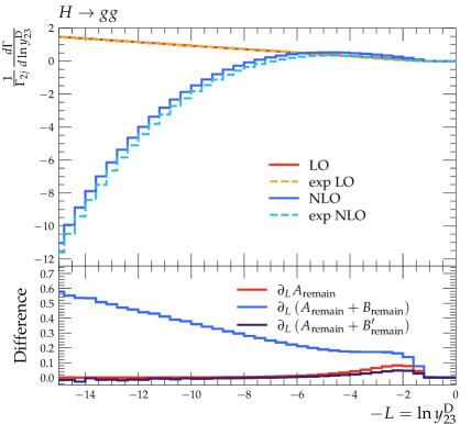
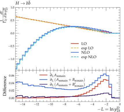
Figure 2: Comparison of the LO and NLO predictions with the corresponding expansion of the resummed result for the case of the Durham jet-resolution observable $y^{\mathrm{D}}_{\mathrm{23}}$ for the $H\to gg$ (left) and $H\to b\bar{b}$ (right) Higgs decay modes. The lower panels show the difference between the fixed-order calculation and the expanded resummation, at order $\alpha_{\text{s}}$ (red), $\alpha_{\text{s}}^{2}$ (blue), and when including the numerically extracted $\mathcal{C}_{1}$ coefficient (purple), see Eqs. (19), (20), and (22) for the definitions of $A_{\text{remain}}$, $B_{\text{remain}}$ and $B^{\prime}_{\text{remain}}$, respectively.

Moving on to the NLO prediction and the expansion of the resummed result up to ${\cal{O}}(\alpha_{\text{s}}^{2})$, shown as solid dark and dashed light blue lines in Fig. 2, we can first remark that they exhibit a qualitatively similar behaviour as at LO, however, now diverging towards $-\infty$. As expected, they do not exactly agree in the soft limit as the NLL resummation is missing subleading logarithmic contributions at this order. By considering again the difference in this kinematic limit, we observe a linearly rising difference, as can be expected from Eq. (20) (note we are here plotting the respective derivatives of the quantities defined there). This artefact is much more prominent in the $H\to gg$ case, where a linear rise from $0.3$ to $0.6$ can be observed in the range $L=8$ to $L=15$, whereas the remainder in the $H\to b\bar{b}$ case only increases by $0.01$ over the same range. Of course this has to be considered in relation to the fact that the whole distribution in the second case is shifted towards larger logarithms, due to the smaller colour factors involved in the case of Higgs decays to quarks. We hence argue that this behaviour is qualitatively consistent with Casimir scaling. We have checked that the difference in $H\to b\bar{b}$ indeed continues with a logarithmic rise, at least within the statistical uncertainties of the numerical evaluation, until a value of $L=20$. Fluctuations do become large in this regime and we hence limit the plot range as shown in the figure.

As argued before, our multiplicative matching scheme incorporates an effective coefficient $A_{0}\equiv\mathcal{C}_{1}$, which captures the leading part of this disagreement. This is illustrated in the lower panels by the purple curves, where we subtract all the terms that are present to ${\cal{O}}(\alpha_{\text{s}}^{2})$ in our matched predictions, cf. Eq. (22). We should stress that, while the remaining difference indeed approaches a numerically small value, the two results still mismatch by a constant term corresponding to an uncontrolled ${\cal{O}}(\alpha_{\text{s}}^{2}L)$ contribution to $\Gamma_{gg}$ and $\Gamma_{b\bar{b}}$ that could only be captured by a NNLL accurate resummed calculation. These observations hold for both cases, $H\to gg$ and $H\to b\bar{b}$, in Fig. 2.

An overview of the same validation for the remaining observables can be found in Fig. 3. For the traditional (ungroomed) observables, i.e., thrust $\tau$, $C$-parameter, scaled heavy-jet mass $\rho_{\mathrm{H}}$, total and wide jet broadening, we find a similar picture as expected. Again, the linear rise in the uncorrected remainder at NLO (shown in blue) is much more prominent in the Higgs decaying to gluons decay mode, however for several observables, the linear behaviour can unambiguously be identified also in the case where the Higgs boson decays into quarks. Further, we note that for some observables like the $C$-parameter and the broadenings we now indeed observe non-vanishing constant differences in $B^{\prime}_{\text{remain}}$ (purple lines). While these have a positive sign for the $C$-parameter in both Higgs-decay categories, they exhibit a similar magnitude but with negative sign for both $B_{\text{W}}$ and $B_{\text{T}}$.

We furthermore show results for soft-drop thrust for $z_{\text{cut}}=0.1$ and $\beta=0,1,2$ in Fig. 3. In the groomed distributions, the logarithmic structure is changed. For $\beta=0$, the leading logarithms in $\ln 1/v$ are entirely replaced by logarithms of type $\ln 1/z_{\text{cut}}$, so that the remainder is constant even without the inclusion of the additional terms in $B^{\prime}_{\text{NLL}}$. In general, terms of this order are suppressed by powers of $\beta$. So for $\beta>0$ the linearly rising behaviour of the remainder $B_{\text{remain}}$ is restored, and again fixed by including the additional terms in $B^{\prime}_{\text{remain}}$.

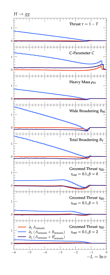
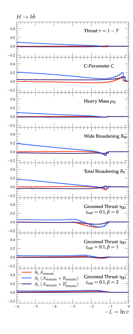
Figure 3: Residual differences between the LO and NLO calculation and the expanded resummation, at order $\alpha_{\text{s}}$ (red), $\alpha_{\text{s}}^{2}$ (blue), and when including the numerically extracted ${\cal{C}}_{1}$ coefficient (purple). For the various observables the left panel contains the results for the case $H\to gg$, while the right panel corresponds to $H\to b\bar{b}$.

4 NLO+NLL’ accurate predictions

We now move to the presentation of our final results, the matched distributions for event-shape observables at NLO accuracy which after the multiplicative combination with the NLL results ultimately achieve $\text{NLO}+\text{NLL}^{\prime}$ precision. We thereby consider the following hadronic Higgs-decay observables: thrust, the $C$-parameter, the heavy-hemisphere mass, total and wide jet broadening, and the Durham three-jet resolution variable $y^{\mathrm{D}}_{23}$. Furthermore, we here present predictions for soft-drop thrust [66] for three values of the soft-drop angular parameter $\beta$, namely $\beta=0,1,2$. The results for those distributions are presented in Figs. 4–6. Each of these figures, or sub-figures, consists of two panels, with the upper panel showing the event-shape distribution and the lower panel presenting the difference between the respective $\text{NLO}+\text{NLL}^{\prime}$ and $\text{LO}+\text{NLL}^{\prime}$ results.

Unlike for the presentation of results in Fig. 2 and Fig. 3, results for both Higgs decay categories, $H\to b\bar{b}$ and $H\to gg$, are presented together in the two panels of Figs. 4–6. The colour scheme in both panels is as follows: Results for the $H\to b\bar{b}$ decay mode are represented in red, while those associated to the $H\to gg$ decay mode are shown in blue.

To estimate theoretical uncertainties, we consider variations by factors of two around the central renormalisation-scale choice $\mu_{\text{R}}=m_{H}$, thereby assuming $m_{H}=125~{}\text{GeV}$, corresponding to the alternative choices $\mu_{\text{R}}=2m_{H}$ and $\mu_{\text{R}}=m_{H}/2$. Similarly, we can vary the logarithm to be resummed to $L\to\ln(x_{L}/v)$ while subtracting the additional induced NLL terms to retain our logarithmic accuracy, see for example [89] for details. We likewise vary $x_{L}$ around our default $x_{L}=1$ to $x_{L}=2$ and $x_{L}=1/2$. Keeping the two variations separate, we overall obtain 5 results and their spread is indicated in both panels, for the $H\to b\bar{b}$ decay mode by the red and for the $H\to gg$ mode by the blue shaded bands, respectively.

The impact of NLO corrections is best illustrated in the lower panels of Figs. 4–6. The uncertainty bands in these cases indicate the difference between the alternative scale choices in the $\text{NLO}+\text{NLL}^{\prime}$ and the central $\text{LO}+\text{NLL}^{\prime}$ predictions.

For the central scale choice, we observe the largest NLO corrections towards the kinematical endpoints, i.e., for rather large observable values. This is in line with expectations, because real-radiation corrections open up the phase space in the multi-particle limit, located towards the right-hand side of the figures. As such, event-shape observables are dominated by the real contribution of the NLO corrections there. Close inspection reveals that in these phase-space regions, the uncertainty bands of the LO- and NLO-matched distributions do not overlap. This is consistent with the observations made for the (unmatched) fixed-order predictions presented in [63], i.e., that the LO distributions receive large NLO corrections in both Higgs-decay channels. In the limit of large logarithms, located on the left-hand side of the figures, the differences between NLO- and LO-matched distributions are approaching zero, since both distributions are smoothly vanishing in that region. This is a requirement on physical distributions and ensured by our multiplicative matching scheme, cf. Eq. (17).

Comparing the results obtained in both Higgs-decay categories, the following general statements hold. As expected from Casimir scaling, the distributions in the $H\to gg$ decay mode are shifted towards significantly higher values for all the event shapes considered here. Only for the $\tau_{\text{SD}}$ distribution, this observation is broken to some extent, as soft-drop grooming here significantly sculpts the $H\to b\bar{b}$ result.

For soft-drop thrust there appears a transition point between the groomed and largely ungroomed region at $\tau_{\mathrm{SD}}=z_{\text{cut}}2^{\beta/2}$ [66]. For $z_{\text{cut}}=0.1$ as employed here, this is numerically close to the peak of the $H\to gg$ distribution, e.g., for $\beta=0$ this corresponds to $\ln\tau_{\text{SD}}\approx-2.3$. For rather strong grooming, in particular when using $\beta=0$, the quark distribution is significantly suppressed below the transition point and in consequence develops a peak at larger values, close to the maximum of the $H\to gg$ distribution. Interestingly, while the distributions related to the Higgs to gluon decay mode approach zero much earlier than those related to the Higgs to quark decay mode, as seen in the upper panels of the figures, this is not necessarily the case for the difference between the respective LO- and NLO-matched distributions, shown in the lower panels.

In Fig. 4 we present results for the mass-like thrust $\tau$ with C AESAR parameters $a=1$, $b=1$ and its soft-drop groomed variant $\tau_{\mathrm{SD}}$. As mentioned before, for both observables we present the distributions containing results for the gluonic $H\to gg$ decays as well as for the decays to $b$-quarks, in the same plot. In the groomed case, the difference above the transition point $\tau_{\text{SD}}\sim z_{\text{cut}}=0.1$ appears to be somewhat larger than in the equivalent region of the ungroomed thrust. There appears a non-smooth feature around the transition point, i.e., $\ln\tau_{\text{SD}}\approx-2.3$, which in particular for the $H\to gg$ case is more visible in the difference than in the actual distribution. Below this point the difference to the leading-order matched distribution quickly decays. In the ungroomed cases an oscillating behaviour is seen instead, with the difference transitioning between positive and negative values, with vanishing absolute value. We can observe in the two panels of Fig. 4 that the leading-order matched result appears to be within the error band of the $\text{NLO}+\text{NLL}^{\prime}$ result. The only exceptions are the points where the band boundaries cross each other, as expected for normalised distributions. We conclude that, taking into account the uncertainty estimates, the $\text{LO}+\text{NLL}^{\prime}$ and $\text{NLO}+\text{NLL}^{\prime}$ results are compatible.

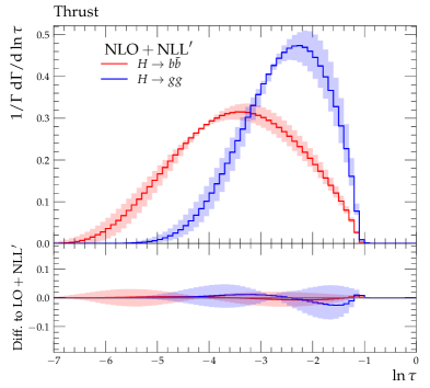
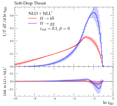
Figure 4: Matched NLO+NLL^′ predictions for standard and soft-drop groomed thrust with $\beta=0$. The lower panels contain the difference between the respective $\text{NLO}+\text{NLL}^{\prime}$ and $\text{LO}+\text{NLL}^{\prime}$ results (see text).

In Fig. 5, we show our predictions for the transverse-momentum-like total broadening $B_{\mathrm{T}}$ with C AESAR parameters $a=1,b=0$. The general hierarchy between the $H\to gg$ and $H\to b\bar{b}$ cases is evident. We observe slightly larger corrections in the difference between NLO- and LO-matched results in the lower panel. In this case, the difference for gluon-initiated events indeed decays faster, just as the overall distributions. Otherwise we observe a similar oscillating behaviour as in the ungroomed thrust case. Close inspection of the hard phase-space region on the far right-hand side of the plot again shows that the uncertainty bands at LO and NLO do not overlap. As alluded to above, this is consistent with the findings in [63]. The distribution is dominated by the real corrections at the hard kinematical endpoint.

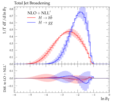
Figure 5: Matched NLO+NLL^′ predictions for total broadening. The lower panel contains the difference between the respective $\text{NLO}+\text{NLL}^{\prime}$ and $\text{LO}+\text{NLL}^{\prime}$ results (see text).

In Fig. 6, we present corresponding results for the remaining observables, i.e., for the $C$-parameter, wide jet broadening, heavy-hemisphere mass, Durham three-jet resolution, and soft-drop thrust with $\beta=1,2$. Qualitatively, we observe a similar impact of the NLO corrections as for thrust and total jet broadening, cf. Figs. 4 and 5. The largest NLO corrections in the difference can be seen for the $C$-parameter. This is dominated by the Sudakov shoulder effects [111, 23, 37, 38] around the kinematic endpoints, i.e., the far-right side of the figure. These effects emphasise that the respective leading-order results are not covered by the NLO uncertainty band. In this context, it is to be highlighted that all event-shape distributions shown here are dominated by the $\text{NLL}^{\prime}$ resummation in the soft region, $\ln v\lesssim-2$ and by the fixed-order calculation in the hard region, $\ln v\gtrsim-2$. As expected, the heavy-jet mass behaves very similar to thrust; we note that they agree for three-particle configurations. Likewise, we observe a similar behaviour of the wide jet broadening $B_{\mathrm{W}}$ as for the closely related total jet broadening $B_{\mathrm{T}}$.

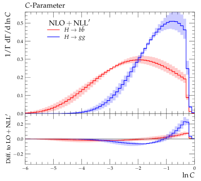
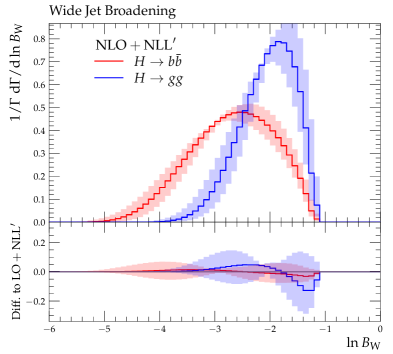
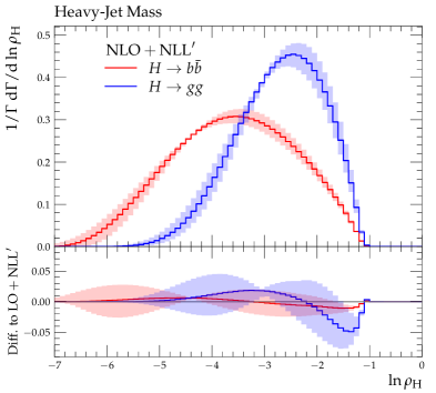
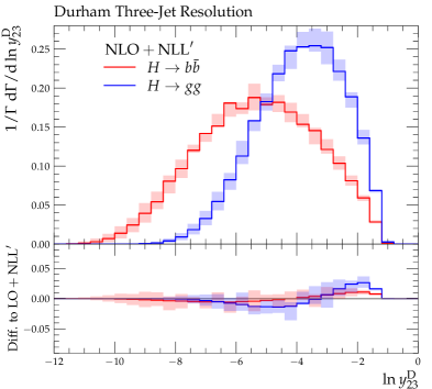
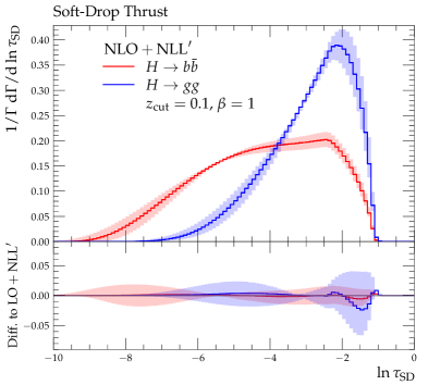
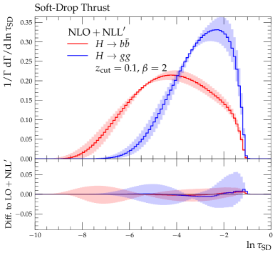
Figure 6: Matched NLO+NLL^′ predictions for $C$-parameter and heavy-jet mass (top row), wide broadening and Durham jet resolution (middle row), and soft-drop groomed thrust with $\beta=1,2$ (bottom row). The lower panels contain the difference between the respective $\text{NLO}+\text{NLL}^{\prime}$ and $\text{LO}+\text{NLL}^{\prime}$ results (see text).

We note that the Durham three-jet resolution $y^{\mathrm{D}}_{\mathrm{23}}$ has a similar scaling as the broadenings, however with $a=2,b=0$. This corresponds to a factor two on the logarithm on the abscissa and we thus extend the plot range correspondingly. The corrections from matching appear to be generally smaller in this case than the others, in agreement with [63]. In particular we do not observe any marked features around the kinematical endpoint.

In the lowest row of Fig. 6, we finally show the results for soft-drop groomed thrust with two different values of $\beta=1$ and $\beta=2$, corresponding to a less aggressive grooming, compared to the case $\beta=0$. For the first case we observe a transition behaviour with a peak at higher values in the $H\to b\bar{b}$ distribution, moving the peak position closer to that of the $H\to gg$ case. For $\beta=2$, the grooming is weak enough to allow for the development of the usual Sudakov peak, and we hence observe a cleaner separation of the two distributions. The effects from NLO matching compared to LO appear to be smaller again for these two groomed thrust variants. There are also no easily identifiable features around the transition point anymore in the difference shown in the lower panels. We only observe slight differences towards the kinematical endpoint, which then vanish very fast with increasing logarithm $L$, at least compared to the other cases we studied.

5 Conclusions

Further scrutinising the Standard Model of particle physics through precision measurements of Higgs-boson couplings forms a central task for experiments at a possible future lepton collider. This in particular includes studies of hadronic Higgs-boson decays that ultimately might provide access to an extraction of the Higgs-gluon-gluon coupling. Event-shape observables offer a discriminatory power between the various possible hadronic Higgs-boson decay channels, and in particular between the decay modes $H\to b\bar{b}$ and $H\to gg$, thereby being largely complementary to techniques that instrument displaced vertices due to weak decays of flavourful hadrons.

We have here presented resummed predictions at $\text{NLO}+\text{NLL}^{\prime}$ accuracy for an extended set of three-jet event-shape observables for these two hadronic decay modes. Besides the event-shape observables thrust, $C$-parameter, total and wide jet broadenings, heavy-hemisphere mass, and the three-jet resolution in the Durham jet clustering algorithm, we here also considered soft-drop groomed thrust. Building on next-to-leading order calculations compiled with E ERAD 3, first presented in [63], we extended those to soft-drop thrust and combined them with an all-orders resummation of next-to-leading logarithms in the observables. To this end, we have used the implementation of the C AESAR resummation formalism in the S HERPA event-generator framework. Based on a multiplicative matching scheme we were able to achieve $\text{NLO}+\text{NLL}^{\prime}$ accuracy for the differential distributions of the considered event-shape observables. We have carefully cross checked our fixed-order and resummed calculations through a detailed comparison in softly and collinearly enhanced kinematic configurations, i.e., for the case of very small observable values.

The results presented here extend the fixed-order predictions of [63] to phase-space regions in which event-shape observables receive large logarithmic corrections from soft and collinear three-particle configurations. In the deep infrared region, at scales of the order of $\Lambda_{\mathrm{QCD}}$, observables further receive important non-perturbative corrections from the long-range behaviour of QCD. Hadronisation corrections are not included in our predictions, but it can be anticipated that the impact of these can be reduced by utilising grooming techniques, as done for the soft-drop thrust in the present work, see e.g., [110, 66, 88].

In line with expectations, we find the impact of NLO corrections to be small over the bulk of the logarithmic observable range. Considerable differences to the leading-order-matched predictions are only found in the hard phase-space region. The largest corrections were found for the $C$-parameter, amplified by the presence of large Sudakov-shoulder effects, followed by the heavy-jet mass $\rho_{\mathrm{H}}$. The smallest NLO corrections are present in the soft-drop thrust distributions, for all three values of $\beta$ studied. For almost all event-shape observables considered here, we observe the expected behaviour that distributions in $H\to gg$ decays peak at considerably larger observable values than in $H\to b\bar{b}$ decays. This is only altered by grooming, which results in a shift of the peak in $H\to b\bar{b}$ distributions towards larger observable values for $\beta=0$ and $1$. While we have here focussed on the six “classical” event shapes, including a groomed version of thrust, our implementation straightforwardly extends to other (infrared-safe) observables, so long as they fall in the category of being treatable by the C AESAR formalism. A particular class of observables to mention are fractional moments of energy–energy correlators $\mathrm{FC}_{x}$ [64, 36, 112] that recently were also considered in the context of discriminating hadronic Higgs-boson decays [15].

Our work marks an important step towards precision calculations for Higgs-boson studies at future lepton colliders, provides important benchmarks for the assessment [113, 114, 115, 116] and development [117, 118, 107, 119, 120, 121] of parton-shower algorithms with higher logarithmic accuracy and can serve as theoretical input into jet-flavour tagging studies. To further improve the formal accuracy of predictions pertaining to three-jet event-shapes, next-to-next-to-leading order (NNLO) corrections need to be evaluated, matching the case of $\gamma^{*}/Z\to q\bar{q}$. To this end, all contributions, especially one- and two-loop amplitudes, needed for NNLO corrections to three-jet observables in $H\to b\bar{b}$ decays [82, 122, 123] and $H\to gg$ decays [82, 124, 125, 126, 127, 128, 129, 130, 131] are known in fully analytic form. Similarly, the resummation should be lifted to the next-to-next-to-leading logarithmic level, e.g., using the A RES  [35] framework. When combined, NNLO+NNLL’ accuracy could be achieved, resulting in a further reduction of theoretical uncertainties. For certain “simple” observables, like thrust, $\text{NNLO}+\text{N}^{3}\text{LL}$ is within reach. Relevant for the $H\to b\bar{b}$ channel, progress has been reported on the inclusion of finite-mass effects, affecting the radiation pattern, in resummed calculations [132, 133, 134, 135].

References

- [1] A. Abada et al., The FCC collaboration, FCC Physics Opportunities: Future Circular Collider Conceptual Design Report Volume 1, Eur. Phys. J. C 79 (2019), no. 6, 474
- [2] A. Abada et al., The FCC collaboration, FCC-ee: The Lepton Collider: Future Circular Collider Conceptual Design Report Volume 2, Eur. Phys. J. ST 228 (2019), no. 2, 261–623
- [3] M. Dong et al., The CEPC Study Group collaboration, CEPC Conceptual Design Report: Volume 2 - Physics & Detector, arXiv:1811.10545 [hep-ex]
- [4] The ILC collaboration, The International Linear Collider Technical Design Report - Volume 2: Physics, arXiv:1306.6352 [hep-ph]
- [5] G. Aad et al., The ATLAS collaboration, Observation of a new particle in the search for the Standard Model Higgs boson with the ATLAS detector at the LHC, Phys. Lett. B 716 (2012), 1–29, [arXiv:1207.7214 [hep-ex]]
- [6] S. Chatrchyan et al., The CMS collaboration, Observation of a New Boson at a Mass of 125 GeV with the CMS Experiment at the LHC, Phys. Lett. B 716 (2012), 30–61, [arXiv:1207.7235 [hep-ex]]
- [7] A. M. Sirunyan et al., The CMS collaboration, Observation of Higgs boson decay to bottom quarks, Phys. Rev. Lett. 121 (2018), no. 12, 121801, [arXiv:1808.08242 [hep-ex]]
- [8] G. Aad et al., The ATLAS collaboration, Measurement of the associated production of a Higgs boson decaying into -quarks with a vector boson at high transverse momentum in collisions at TeV with the ATLAS detector, Phys. Lett. B 816 (2021), 136204, [arXiv:2008.02508 [hep-ex]]
- [9] A. M. Sirunyan et al., The CMS collaboration, A search for the standard model Higgs boson decaying to charm quarks, JHEP 03 (2020), 131, [arXiv:1912.01662 [hep-ex]]
- [10] G. Aad et al., The ATLAS collaboration, Direct constraint on the Higgs-charm coupling from a search for Higgs boson decays into charm quarks with the ATLAS detector, Eur. Phys. J. C 82 (2022), 717, [arXiv:2201.11428 [hep-ex]]
- [11] J. Gao, Probing light-quark Yukawa couplings via hadronic event shapes at lepton colliders, JHEP 01 (2018), 038, [arXiv:1608.01746 [hep-ph]]
- [12] J. Gao, Y. Gong, W.-L. Ju and L. L. Yang, Thrust distribution in Higgs decays at the next-to-leading order and beyond, JHEP 03 (2019), 030, [arXiv:1901.02253 [hep-ph]]
- [13] M.-X. Luo, V. Shtabovenko, T.-Z. Yang and H. X. Zhu, Analytic Next-To-Leading Order Calculation of Energy-Energy Correlation in Gluon-Initiated Higgs Decays, JHEP 06 (2019), 037, [arXiv:1903.07277 [hep-ph]]
- [14] J. Gao, V. Shtabovenko and T.-Z. Yang, Energy-energy correlation in hadronic Higgs decays: analytic results and phenomenology at NLO, JHEP 02 (2021), 210, [arXiv:2012.14188 [hep-ph]]
- [15] M. Knobbe, F. Krauss, D. Reichelt and S. Schumann, Measuring hadronic Higgs boson branching ratios at future lepton colliders, Eur. Phys. J. C 84 (2024), no. 1, 83, [arXiv:2306.03682 [hep-ph]]
- [16] X.-R. Wang and B. Yan, Probing the Hgg coupling through the jet charge correlation in Higgs boson decay, Phys. Rev. D 108 (2023), no. 5, 056010, [arXiv:2302.02084 [hep-ph]]
- [17] D. Decamp et al., The ALEPH collaboration, Measurement of the strong coupling constant alpha-s from global event shape variables of hadronic Z decays, Phys. Lett. B 255 (1991), 623–633
- [18] M. Z. Akrawy et al., The OPAL collaboration, A Measurement of Global Event Shape Distributions in the Hadronic Decays of the , Z. Phys. C 47 (1990), 505–522
- [19] O. Adrian et al., The L3 collaboration, Determination of alpha-s from hadronic event shapes measured on the Z0 resonance, Phys. Lett. B 284 (1992), 471–481
- [20] P. Abreu et al., The DELPHI collaboration, Energy dependence of event shapes and of alpha(s) at LEP-2, Phys. Lett. B 456 (1999), 322–340
- [21] J. Abdallah et al., The DELPHI collaboration, A Study of the energy evolution of event shape distributions and their means with the DELPHI detector at LEP, Eur. Phys. J. C 29 (2003), 285–312, [hep-ex/0307048]
- [22] D. d’Enterria et al., The strong coupling constant: State of the art and the decade ahead, arXiv:2203.08271 [hep-ph]
- [23] A. Gehrmann-De Ridder, T. Gehrmann, E. W. N. Glover and G. Heinrich, NNLO corrections to event shapes in annihilation, JHEP 12 (2007), 094, [arXiv:0711.4711 [hep-ph]]
- [24] A. Gehrmann-De Ridder, T. Gehrmann, E. W. N. Glover and G. Heinrich, NNLO moments of event shapes in annihilation, JHEP 05 (2009), 106, [arXiv:0903.4658 [hep-ph]]
- [25] A. Gehrmann-De Ridder, T. Gehrmann, E. W. N. Glover and G. Heinrich, EERAD3: Event shapes and jet rates in electron-positron annihilation at order , Comput. Phys. Commun. 185 (2014), 3331, [arXiv:1402.4140 [hep-ph]]
- [26] S. Weinzierl, The infrared structure of jets at NNLO reloaded, JHEP 07 (2009), 009, [arXiv:0904.1145 [hep-ph]]
- [27] S. Weinzierl, Event shapes and jet rates in electron-positron annihilation at NNLO, JHEP 06 (2009), 041, [arXiv:0904.1077 [hep-ph]]
- [28] S. Weinzierl, Moments of event shapes in electron-positron annihilation at NNLO, Phys. Rev. D 80 (2009), 094018, [arXiv:0909.5056 [hep-ph]]
- [29] V. Del Duca, C. Duhr, A. Kardos, G. Somogyi, Z. Szőr, Z. Trócsányi and Z. Tulipánt, Jet production in the CoLoRFulNNLO method: event shapes in electron-positron collisions, Phys. Rev. D 94 (2016), no. 7, 074019, [arXiv:1606.03453 [hep-ph]]
- [30] A. Kardos, G. Somogyi and Z. Trócsányi, Soft-drop event shapes in electron–positron annihilation at next-to-next-to-leading order accuracy, Phys. Lett. B 786 (2018), 313–318, [arXiv:1807.11472 [hep-ph]]
- [31] T. Becher, G. Bell and M. Neubert, Factorization and Resummation for Jet Broadening, Phys. Lett. B 704 (2011), 276–283, [arXiv:1104.4108 [hep-ph]]
- [32] T. Becher and G. Bell, NNLL Resummation for Jet Broadening, JHEP 11 (2012), 126, [arXiv:1210.0580 [hep-ph]]
- [33] M. Balsiger, T. Becher and D. Y. Shao, NLL′ resummation of jet mass, JHEP 04 (2019), 020, [arXiv:1901.09038 [hep-ph]]
- [34] A. H. Hoang, D. W. Kolodrubetz, V. Mateu and I. W. Stewart, -parameter distribution at N3LL’ including power corrections, Phys. Rev. D 91 (2015), no. 9, 094017, [arXiv:1411.6633 [hep-ph]]
- [35] A. Banfi, H. McAslan, P. F. Monni and G. Zanderighi, A general method for the resummation of event-shape distributions in annihilation, JHEP 05 (2015), 102, [arXiv:1412.2126 [hep-ph]]
- [36] A. Banfi, B. K. El-Menoufi and P. F. Monni, The Sudakov radiator for jet observables and the soft physical coupling, JHEP 01 (2019), 083, [arXiv:1807.11487 [hep-ph]]
- [37] A. Bhattacharya, M. D. Schwartz and X. Zhang, Sudakov shoulder resummation for thrust and heavy jet mass, Phys. Rev. D 106 (2022), no. 7, 074011, [arXiv:2205.05702 [hep-ph]]
- [38] A. Bhattacharya, J. K. L. Michel, M. D. Schwartz, I. W. Stewart and X. Zhang, NNLL resummation of Sudakov shoulder logarithms in the heavy jet mass distribution, JHEP 11 (2023), 080, [arXiv:2306.08033 [hep-ph]]
- [39] T. Gehrmann, M. Jaquier and G. Luisoni, Hadronization effects in event shape moments, Eur. Phys. J. C 67 (2010), 57–72, [arXiv:0911.2422 [hep-ph]]
- [40] G. Luisoni, P. F. Monni and G. P. Salam, -parameter hadronisation in the symmetric 3-jet limit and impact on fits, Eur. Phys. J. C 81 (2021), no. 2, 158, [arXiv:2012.00622 [hep-ph]]
- [41] F. Caola, S. Ferrario Ravasio, G. Limatola, K. Melnikov and P. Nason, On linear power corrections in certain collider observables, JHEP 01 (2022), 093, [arXiv:2108.08897 [hep-ph]]
- [42] F. Caola, S. Ferrario Ravasio, G. Limatola, K. Melnikov, P. Nason and M. A. Ozcelik, Linear power corrections to e+e– shape variables in the three-jet region, JHEP 12 (2022), 062, [arXiv:2204.02247 [hep-ph]]
- [43] N. Agarwal, M. van Beekveld, E. Laenen, S. Mishra, A. Mukhopadhyay and A. Tripathi, Next-to-leading power corrections to the event shape variables, arXiv:2306.17601 [hep-ph]
- [44] A. Buckley et al., General-purpose event generators for LHC physics, Phys. Rept. 504 (2011), 145–233, [arXiv:1101.2599 [hep-ph]]
- [45] J. M. Campbell et al., Event Generators for High-Energy Physics Experiments, arXiv:2203.11110 [hep-ph]
- [46] A. Banfi, G. P. Salam and G. Zanderighi, Infrared safe definition of jet flavor, Eur. Phys. J. C47 (2006), 113–124, [arXiv:hep-ph/0601139 [hep-ph]]
- [47] P. T. Komiske, E. M. Metodiev and J. Thaler, An operational definition of quark and gluon jets, JHEP 11 (2018), 059, [arXiv:1809.01140 [hep-ph]]
- [48] S. Caletti, O. Fedkevych, S. Marzani, D. Reichelt, S. Schumann, G. Soyez and V. Theeuwes, Jet angularities in Z+jet production at the LHC, JHEP 07 (2021), 076, [arXiv:2104.06920 [hep-ph]]
- [49] S. Caletti, A. J. Larkoski, S. Marzani and D. Reichelt, A fragmentation approach to jet flavor, JHEP 10 (2022), 158, [arXiv:2205.01117 [hep-ph]]
- [50] S. Caletti, A. J. Larkoski, S. Marzani and D. Reichelt, Practical jet flavour through NNLO, Eur. Phys. J. C 82 (2022), no. 7, 632, [arXiv:2205.01109 [hep-ph]]
- [51] M. Czakon, A. Mitov and R. Poncelet, Infrared-safe flavoured anti-kT jets, JHEP 04 (2023), 138, [arXiv:2205.11879 [hep-ph]]
- [52] R. Gauld, A. Huss and G. Stagnitto, Flavor Identification of Reconstructed Hadronic Jets, Phys. Rev. Lett. 130 (2023), no. 16, 161901, [arXiv:2208.11138 [hep-ph]]
- [53] F. Caola, R. Grabarczyk, M. L. Hutt, G. P. Salam, L. Scyboz and J. Thaler, Flavored jets with exact anti-kt kinematics and tests of infrared and collinear safety, Phys. Rev. D 108 (2023), no. 9, 094010, [arXiv:2306.07314 [hep-ph]]
- [54] J. R. Andersen et al., Les Houches 2015: Physics at TeV Colliders Standard Model Working Group Report, arXiv:1605.04692 [hep-ph]
- [55] P. Gras, S. Höche, D. Kar, A. Larkoski, L. Lönnblad, S. Plätzer, A. Siódmok, P. Skands, G. Soyez and J. Thaler, Systematics of quark/gluon tagging, JHEP 07 (2017), 091, [arXiv:1704.03878 [hep-ph]]
- [56] J. Mo, F. J. Tackmann and W. J. Waalewijn, A case study of quark-gluon discrimination at NNLL’ in comparison to parton showers, Eur. Phys. J. C 77 (2017), no. 11, 770, [arXiv:1708.00867 [hep-ph]]
- [57] D. Reichelt, P. Richardson and A. Siodmok, Improving the Simulation of Quark and Gluon Jets with Herwig 7, Eur. Phys. J. C 77 (2017), no. 12, 876, [arXiv:1708.01491 [hep-ph]]
- [58] J. Zhu, Y. Song, J. Gao, D. Kang and T. Maji, Angularity in Higgs boson decays via at NNLL accuracy, arXiv:2311.07282 [hep-ph]
- [59] B. Yan and C. Lee, Probing light quark Yukawa couplings through angularity distributions in Higgs boson decay, arXiv:2311.12556 [hep-ph]
- [60] S. Alioli, A. Broggio, A. Gavardi, S. Kallweit, M. A. Lim, R. Nagar, D. Napoletano and L. Rottoli, Resummed predictions for hadronic Higgs boson decays, JHEP 04 (2021), 254, [arXiv:2009.13533 [hep-ph]]
- [61] Y. Hu, C. Sun, X.-M. Shen and J. Gao, Hadronic decays of Higgs boson at NNLO matched with parton shower, JHEP 08 (2021), 122, [arXiv:2101.08916 [hep-ph]]
- [62] W. Bizoń, E. Re and G. Zanderighi, NNLOPS description of the decay with MiNLO, JHEP 06 (2020), 006, [arXiv:1912.09982 [hep-ph]]
- [63] G. Coloretti, A. Gehrmann-De Ridder and C. T. Preuss, QCD predictions for event-shape distributions in hadronic Higgs decays, JHEP 06 (2022), 009, [arXiv:2202.07333 [hep-ph]]
- [64] A. Banfi, G. P. Salam and G. Zanderighi, Principles of general final-state resummation and automated implementation, JHEP 03 (2005), 073, [arXiv:hep-ph/0407286 [hep-ph]]
- [65] E. Gerwick, S. Höche, S. Marzani and S. Schumann, Soft evolution of multi-jet final states, JHEP 02 (2015), 106, [arXiv:1411.7325 [hep-ph]]
- [66] S. Marzani, D. Reichelt, S. Schumann, G. Soyez and V. Theeuwes, Fitting the Strong Coupling Constant with Soft-Drop Thrust, JHEP 11 (2019), 179, [arXiv:1906.10504 [hep-ph]]
- [67] J. R. Ellis, M. K. Gaillard and D. V. Nanopoulos, A Phenomenological Profile of the Higgs Boson, Nucl. Phys. B 106 (1976), 292
- [68] M. A. Shifman, A. I. Vainshtein, M. B. Voloshin and V. I. Zakharov, Low-Energy Theorems for Higgs Boson Couplings to Photons, Sov. J. Nucl. Phys. 30 (1979), 711–716
- [69] B. A. Kniehl and M. Spira, Low-energy theorems in Higgs physics, Z. Phys. C 69 (1995), 77–88, [hep-ph/9505225]
- [70] T. Inami, T. Kubota and Y. Okada, Effective Gauge Theory and the Effect of Heavy Quarks in Higgs Boson Decays, Z. Phys. C 18 (1983), 69–80
- [71] A. Djouadi, J. Kalinowski and P. M. Zerwas, Higgs radiation off top quarks in high-energy colliders, Z. Phys. C 54 (1992), 255–262
- [72] K. G. Chetyrkin, B. A. Kniehl and M. Steinhauser, Hadronic Higgs decay to order alpha-s**4, Phys. Rev. Lett. 79 (1997), 353–356, [hep-ph/9705240]
- [73] K. G. Chetyrkin, B. A. Kniehl and M. Steinhauser, Decoupling relations to O (alpha-s**3) and their connection to low-energy theorems, Nucl. Phys. B 510 (1998), 61–87, [hep-ph/9708255]
- [74] K. G. Chetyrkin, J. H. Kuhn and C. Sturm, QCD decoupling at four loops, Nucl. Phys. B 744 (2006), 121–135, [hep-ph/0512060]
- [75] Y. Schroder and M. Steinhauser, Four-loop decoupling relations for the strong coupling, JHEP 01 (2006), 051, [hep-ph/0512058]
- [76] P. A. Baikov, K. G. Chetyrkin and J. H. Kühn, Five-Loop Running of the QCD coupling constant, Phys. Rev. Lett. 118 (2017), no. 8, 082002, [arXiv:1606.08659 [hep-ph]]
- [77] S. Brandt, C. Peyrou, R. Sosnowski and A. Wroblewski, The Principal axis of jets. An Attempt to analyze high-energy collisions as two-body processes, Phys. Lett. 12 (1964), 57–61
- [78] E. Farhi, A QCD Test for Jets, Phys. Rev. Lett. 39 (1977), 1587–1588
- [79] A. J. Larkoski, S. Marzani, G. Soyez and J. Thaler, Soft Drop, JHEP 05 (2014), 146, [arXiv:1402.2657 [hep-ph]]
- [80] A. Gehrmann-De Ridder, T. Gehrmann, E. W. N. Glover and G. Heinrich, Jet rates in electron-positron annihilation at in QCD, Phys. Rev. Lett. 100 (2008), 172001, [arXiv:0802.0813 [hep-ph]]
- [81] B. C. Aveleira, A. Gehrmann-De Ridder and C. T. Preuss, A comparative study of flavour-sensitive observables in hadronic Higgs decays, arXiv:2402.17379 [hep-ph]
- [82] A. Gehrmann-De Ridder, C. T. Preuss and C. Williams, Four-jet event shapes in hadronic Higgs decays, arXiv:2310.09354 [hep-ph]
- [83] J. M. Campbell, M. A. Cullen and E. W. N. Glover, Four jet event shapes in electron - positron annihilation, Eur. Phys. J. C 9 (1999), 245–265, [hep-ph/9809429]
- [84] A. Gehrmann-De Ridder, T. Gehrmann and E. W. N. Glover, Antenna subtraction at NNLO, JHEP 09 (2005), 056, [hep-ph/0505111]
- [85] J. Currie, E. W. N. Glover and S. Wells, Infrared Structure at NNLO Using Antenna Subtraction, JHEP 04 (2013), 066, [arXiv:1301.4693 [hep-ph]]
- [86] T. Gleisberg, S. Höche, F. Krauss, M. Schönherr, S. Schumann, F. Siegert and J. Winter, Event generation with SHERPA 1.1, JHEP 02 (2009), 007, [arXiv:0811.4622 [hep-ph]]
- [87] E. Bothmann et al., Event Generation with Sherpa 2.2, SciPost Phys. 7 (2019), no. 3, 034, [arXiv:1905.09127 [hep-ph]]
- [88] J. Baron, D. Reichelt, S. Schumann, N. Schwanemann and V. Theeuwes, Soft-drop grooming for hadronic event shapes, JHEP 07 (2021), 142, [arXiv:2012.09574 [hep-ph]]
- [89] N. Baberuxki, C. T. Preuss, D. Reichelt and S. Schumann, Resummed predictions for jet-resolution scales in multijet production in e+e- annihilation, JHEP 04 (2020), 112, [arXiv:1912.09396 [hep-ph]]
- [90] S. Caletti, O. Fedkevych, S. Marzani and D. Reichelt, Tagging the initial-state gluon, Eur. Phys. J. C 81 (2021), no. 9, 844, [arXiv:2108.10024 [hep-ph]]
- [91] D. Reichelt, S. Caletti, O. Fedkevych, S. Marzani, S. Schumann and G. Soyez, Phenomenology of jet angularities at the LHC, JHEP 03 (2022), 131, [arXiv:2112.09545 [hep-ph]]
- [92] M. Knobbe, D. Reichelt and S. Schumann, (N)NLO+NLL’ accurate predictions for plain and groomed 1-jettiness in neutral current DIS, JHEP 09 (2023), 194, [arXiv:2306.17736 [hep-ph]]
- [93] S. Catani, L. Trentadue, G. Turnock and B. R. Webber, Resummation of large logarithms in event shape distributions, Nucl. Phys. B407 (1993), 3–42
- [94] S. Catani, Y. L. Dokshitzer, M. Olsson, G. Turnock and B. R. Webber, New clustering algorithm for multi-jet cross-sections in annihilation, Phys. Lett. B269 (1991), 432–438
- [95] N. Brown and W. J. Stirling, Jet cross-sections at leading double logarithm in annihilation, Phys. Lett. B 252 (1990), 657–662
- [96] N. Brown and W. J. Stirling, Finding jets and summing soft gluons: A New algorithm, Z. Phys. C 53 (1992), 629–636
- [97] W. J. Stirling, Hard QCD working group: Theory summary, J. Phys. G 17 (1991), 1567–1574
- [98] S. Bethke, Z. Kunszt, D. E. Soper and W. J. Stirling, New jet cluster algorithms: Next-to-leading order QCD and hadronization corrections, Nucl. Phys. B 370 (1992), 310–334, [Erratum: Nucl.Phys.B 523, 681–681 (1998)]
- [99] G. Parisi, Super Inclusive Cross-Sections, Phys. Lett. B 74 (1978), 65–67
- [100] J. F. Donoghue, F. E. Low and S.-Y. Pi, Tensor Analysis of Hadronic Jets in Quantum Chromodynamics, Phys. Rev. D 20 (1979), 2759
- [101] S. Catani, G. Turnock, B. R. Webber and L. Trentadue, Thrust distribution in annihilation, Phys. Lett. B 263 (1991), 491–497
- [102] A. Banfi, G. P. Salam and G. Zanderighi, Semi-numerical resummation of event shapes, JHEP 01 (2002), 018, [arXiv:hep-ph/0112156 [hep-ph]]
- [103] L. Clavelli and D. Wyler, Kinematical Bounds on Jet Variables and the Heavy Jet Mass Distribution, Phys. Lett. B 103 (1981), 383–387
- [104] P. E. L. Rakow and B. R. Webber, Transverse Momentum Moments of Hadron Distributions in QCD Jets, Nucl. Phys. B 191 (1981), 63–74
- [105] S. Catani, G. Turnock and B. R. Webber, Jet broadening measures in annihilation, Phys. Lett. B 295 (1992), 269–276
- [106] Y. L. Dokshitzer, A. Lucenti, G. Marchesini and G. P. Salam, On the QCD analysis of jet broadening, JHEP 01 (1998), 011, [hep-ph/9801324]
- [107] F. Herren, S. Höche, F. Krauss, D. Reichelt and M. Schönherr, A new approach to color-coherent parton evolution, JHEP 10 (2023), 091, [arXiv:2208.06057 [hep-ph]]
- [108] Y. L. Dokshitzer, G. D. Leder, S. Moretti and B. R. Webber, Better jet clustering algorithms, JHEP 08 (1997), 001, [arXiv:hep-ph/9707323 [hep-ph]]
- [109] M. Wobisch and T. Wengler, Hadronization corrections to jet cross-sections in deep inelastic scattering, 270–279, hep-ph/9907280
- [110] J. Baron, S. Marzani and V. Theeuwes, Soft-Drop Thrust, JHEP 08 (2018), 105, [arXiv:1803.04719 [hep-ph]], [Erratum: JHEP 05, 056 (2019)]
- [111] S. Catani and B. R. Webber, Infrared safe but infinite: Soft gluon divergences inside the physical region, JHEP 10 (1997), 005, [hep-ph/9710333]
- [112] M. van Beekveld, M. Dasgupta, B. K. El-Menoufi, J. Helliwell and P. F. Monni, Collinear fragmentation at NNLL: generating functionals, groomed correlators and angularities, arXiv:2307.15734 [hep-ph]
- [113] S. Höche, D. Reichelt and F. Siegert, Momentum conservation and unitarity in parton showers and NLL resummation, JHEP 01 (2018), 118, [arXiv:1711.03497 [hep-ph]]
- [114] M. Dasgupta, F. A. Dreyer, K. Hamilton, P. F. Monni and G. P. Salam, Logarithmic accuracy of parton showers: a fixed-order study, JHEP 09 (2018), 033, [arXiv:1805.09327 [hep-ph]]
- [115] Z. Nagy and D. E. Soper, Summations by parton showers of large logarithms in electron-positron annihilation, arXiv:2011.04777 [hep-ph]
- [116] Z. Nagy and D. E. Soper, Summations of large logarithms by parton showers, Phys. Rev. D 104 (2021), no. 5, 054049, [arXiv:2011.04773 [hep-ph]]
- [117] M. Dasgupta, F. A. Dreyer, K. Hamilton, P. F. Monni, G. P. Salam and G. Soyez, Parton showers beyond leading logarithmic accuracy, Phys. Rev. Lett. 125 (2020), no. 5, 052002, [arXiv:2002.11114 [hep-ph]]
- [118] J. R. Forshaw, J. Holguin and S. Plätzer, Building a consistent parton shower, JHEP 09 (2020), 014, [arXiv:2003.06400 [hep-ph]]
- [119] B. Assi and S. Höche, A new approach to QCD evolution in processes with massive partons, arXiv:2307.00728 [hep-ph]
- [120] K. Hamilton, A. Karlberg, G. P. Salam, L. Scyboz and R. Verheyen, Matching and event-shape NNDL accuracy in parton showers, JHEP 03 (2023), 224, [arXiv:2301.09645 [hep-ph]], [Erratum: JHEP 11, 060 (2023)]
- [121] S. Ferrario Ravasio, K. Hamilton, A. Karlberg, G. P. Salam, L. Scyboz and G. Soyez, Parton Showering with Higher Logarithmic Accuracy for Soft Emissions, Phys. Rev. Lett. 131 (2023), no. 16, 161906, [arXiv:2307.11142 [hep-ph]]
- [122] T. Ahmed, M. Mahakhud, P. Mathews, N. Rana and V. Ravindran, Two-loop QCD corrections to Higgs amplitude, JHEP 08 (2014), 075, [arXiv:1405.2324 [hep-ph]]
- [123] R. Mondini and C. Williams, at next-to-next-to-leading order accuracy, JHEP 06 (2019), 120, [arXiv:1904.08961 [hep-ph]]
- [124] T. Gehrmann, M. Jaquier, E. W. N. Glover and A. Koukoutsakis, Two-Loop QCD Corrections to the Helicity Amplitudes for 3 partons, JHEP 02 (2012), 056, [arXiv:1112.3554 [hep-ph]]
- [125] C. F. Berger, V. Del Duca and L. J. Dixon, Recursive Construction of Higgs-Plus-Multiparton Loop Amplitudes: The Last of the Phi-nite Loop Amplitudes, Phys. Rev. D 74 (2006), 094021, [hep-ph/0608180], [Erratum: Phys.Rev.D 76, 099901 (2007)]
- [126] S. D. Badger and E. W. N. Glover, One-loop helicity amplitudes for H — gluons: The All-minus configuration, Nucl. Phys. B Proc. Suppl. 160 (2006), 71–75, [hep-ph/0607139]
- [127] S. D. Badger, E. W. N. Glover and K. Risager, One-loop phi-MHV amplitudes using the unitarity bootstrap, JHEP 07 (2007), 066, [arXiv:0704.3914 [hep-ph]]
- [128] E. W. N. Glover, P. Mastrolia and C. Williams, One-loop phi-MHV amplitudes using the unitarity bootstrap: The General helicity case, JHEP 08 (2008), 017, [arXiv:0804.4149 [hep-ph]]
- [129] S. Badger, E. W. Nigel Glover, P. Mastrolia and C. Williams, One-loop Higgs plus four gluon amplitudes: Full analytic results, JHEP 01 (2010), 036, [arXiv:0909.4475 [hep-ph]]
- [130] L. J. Dixon and Y. Sofianatos, Analytic one-loop amplitudes for a Higgs boson plus four partons, JHEP 08 (2009), 058, [arXiv:0906.0008 [hep-ph]]
- [131] S. Badger, J. M. Campbell, R. K. Ellis and C. Williams, Analytic results for the one-loop NMHV Hqqgg amplitude, JHEP 12 (2009), 035, [arXiv:0910.4481 [hep-ph]]
- [132] M. Fickinger, S. Fleming, C. Kim and E. Mereghetti, Effective field theory approach to heavy quark fragmentation, JHEP 11 (2016), 095, [arXiv:1606.07737 [hep-ph]]
- [133] D. Gaggero, A. Ghira, S. Marzani and G. Ridolfi, Soft logarithms in processes with heavy quarks, JHEP 09 (2022), 058, [arXiv:2207.13567 [hep-ph]]
- [134] A. Ghira, S. Marzani and G. Ridolfi, A consistent resummation of mass and soft logarithms in processes with heavy flavours, JHEP 11 (2023), 120, [arXiv:2309.06139 [hep-ph]]
- [135] S. Caletti, A. Ghira and S. Marzani, On heavy-flavour jets with Soft Drop, Eur. Phys. J. C 84 (2024), no. 2, 212, [arXiv:2312.11623 [hep-ph]]