Simplicity Bias of Transformers to Learn
Low Sensitivity Functions

Abstract

Transformers achieve state-of-the-art accuracy and robustness across many tasks, but an understanding of the inductive biases that they have and how those biases are different from other neural network architectures remains elusive. Various neural network architectures such as fully connected networks have been found to have a simplicity bias towards simple functions of the data; one version of this simplicity bias is a spectral bias to learn simple functions in the Fourier space. In this work, we identify the notion of sensitivity of the model to random changes in the input as a notion of simplicity bias which provides a unified metric to explain the simplicity and spectral bias of transformers across different data modalities. We show that transformers have lower sensitivity than alternative architectures, such as LSTMs, MLPs and CNNs, across both vision and language tasks. We also show that low-sensitivity bias correlates with improved robustness; furthermore, it can also be used as an efficient intervention to further improve the robustness of transformers.

1 Introduction

Transformers (Vaswani et al.,, 2017) have become a universal backbone in machine learning, and have achieved impressive results across diverse domains including natural language processing (Devlin et al.,, 2019; Brown et al.,, 2020; OpenAI,, 2023), computer vision (Dosovitskiy et al.,, 2021) and protein structure prediction (Jumper et al.,, 2021; Moussad et al.,, 2023). Many recent works have also found that not only do transformers achieve better accuracy, but they are also more robust to various corruptions and changes in the data distribution (Shao et al.,, 2021; Mahmood et al.,, 2021; Bhojanapalli et al.,, 2021; Paul and Chen,, 2022).

Owing to this practical success, there has been significant interest in developing an understanding of how transformers work. Recently, there have been several interesting results onin uncovering the mechanisms by which transformers solve specific algorithmic or prediction tasks (e.g. Wang et al.,, 2022; Hanna et al.,, 2023; Akyürek et al.,, 2023). However, real-world data and prediction tasks are complex and are often not easily modelledmodeled by concrete algorithmic tasks. Therefore, it seems useful to also understand if there are broader classes of functions that transformers prefer to learn from data, and identify high-level inductive biases that they have that hold across multiple types of data.

There have been several recent results in this vein that attempt to understand the inductive biases of neural networks, most of which focus on fully-connected networks. One emerging hypothesis is that neural networks prefer to learn simple functions, and this is termed as ‘simplicity bias’ (Valle-Perez et al.,, 2019; Shah et al.,, 2020; Huh et al.,, 2021; Lyu et al.,, 2021). The starting pointpremise of our work is whether there are appropriate notions of simplicity bias that explain the behavior of transformers in practice. A promising simplicitynotion which has yielded interesting theoretical and practical results for neural networks is spectral bias (Rahaman et al.,, 2019), which is a bias towards simple functions in the Fourier space. Simple functions in the Fourier space generally correspond to low-frequency terms when the input space is continuous, and low-degree polynomials when the input space is discrete. Recent work has shown that deep networks prefer to use low-frequency Fourier functions on images (Xu et al.,, 2019), and low-degree Fourier terms on Boolean functions (Yang and Salman,, 2020). In particular, we are inspired by the work of Bhattamishra et al., 2023b , who find that transformers are biased to learn functions with low sensitivity on Boolean inputs. The sensitivity of a function measures how likely the output is to change for random changes to the input. It is closely related to the Fourier expansion of the function and the weight on low-degree Fourier terms, and also to various other notions of complexity such as the size of the smallest decision tree (O’Donnell,, 2014). Sensitivity has also been found to correlate with better generalization for fully-connected networks (Novak et al.,, 2018). It also has the advantage that it can be efficiently estimated on data through sampling — in contrast, estimating all the Fourier coefficients requires time exponential in the dimensionality of the data and hence can be computationally prohibitive (Xu et al.,, 2019).

Our results.

The goal of our work is to investigate whether sensitivity provides a unified perspective to understand the simplicity bias of transformers across varied data modalities, and if it can help explain properties of transformers such as their improved robustness. We now provide an overview of the main claims and results of the paper. We begin our investigation with the following question:

Do transformers have a bias towards low-sensitivity functions which also holds true beyond Boolean functions?

To answer this, we first show a simple proposition which proves that transformers indeed show a spectral bias on Boolean functions, relying on the work of Yang and Salman, 2020 (Section 3). We then construct a synthetic dataset that demonstrates that transformers prefer to learn low-sensitivity functions on high-dimensional spaces (Section 4). The synthetic setting allows us to tease apart sensitivity from related notions, such as a preference towards functions that depend on a sparse set of tokens. Next, we examine if this low-sensitivity bias is widely present across different tasks:

Does low-sensitivity provide a unified notion of simplicity across vision and language tasks, and does it distinguish between transformers and other architectures?

Here, we first conduct experiments on vision datasets. We empirically compare transformers with MLPs and CNNs and observe that transformers have lower sensitivity compared to other candidate architectures (see Section 5). Similarly, we conduct experiments on language tasks and observe that transformers learn predictors with lower sensitivity than LSTM models. Furthermore, transformers tend to have uniform sensitivity to all tokens while LSTMs are more sensitive to more recent tokens (see Section 6). Given this low-sensitivity bias, we next examine its implications:

What are the implications of a bias towards low-sensitivity functions, and is it helpful in certain settings?

Here, we first show that models with lower sensitivity are more robust to corruptions when tested on the CIFAR-10-C datasets — in particular, transformers have lower sensitivity and are more robust than CNNs (Section 7). We also demonstrate that sensitivity is not only predictive of robustness but also has prescriptive power: We add a regularization term at training time to encourage the model to have lesslower sensitivity. Since sensitivity is efficient to measure empirically, this is easy to accomplish via data augmentation. We find that models explicitly trained to have lower sensitivity yield even better robustness on CIFAR-10-C. Together, our results show that sensitivity provides a general metric to understand the bias of transformers across various tasks, and helps explain properties such as their improved robustness.

Additionally, we explore the connection between sensitivity and a property of the loss landscape that has been found to correlate to good generalization — the sharpness of the minimum. We compare the sharpness of the minima with and without the sensitivity regularization, and our results show that lower sensitivity correlates with flatter minima. This indicates that sensitivity could serve as a unified notion for both robustness and generalization.

2 Related Work

We discuss related work on simplicity bias in deep learning and understanding transformers in this section, and related work on implicit biases of gradient methods, the robustness of transformers and data augmentation in Appendix C.

Simplicity Bias in Deep Learning.

Several works (Neyshabur et al.,, 2014; Valle-Perez et al.,, 2019; Arpit et al.,, 2017; Geirhos et al.,, 2020) show that NNs prefer learning ‘simple’ functions over the data. Nakkiran et al., (2019) show that during the early stages of SGD training, the predictions of NNs can be approximated well by linear models. Morwani et al., (2023) show that 1-hidden-layer NNs exhibit simplicity bias to rely on low-dimensional projections of the data, while Huh et al., (2021) empirically show that deep NNs find solutions with lower rank embeddings. Shah et al., (2020) create synthetic datasets where features that can be separated by predictors with fewer piece-wise linear components are considered simpler, and show that in the presence of simple and complex features with equal predictive power, NNs rely heavily on simple features. Geirhos et al., (2019) show that trained CNNs rely more on image textures rather than image shapes to make predictions. Rahaman et al., (2019) use Fourier analysis tools and show that deep networks are biased towards learning low-frequency functions, and Xu et al., (2019); Cao et al., (2021) provide further theoretical and empirical evidence for this.

Understanding Transformers.

The emergence of transformers as the go-to architecture for many tasks has inspired extensive work on understanding the internal mechanisms of transformers, including reverse-engineering language models (Wang et al.,, 2022), the grokking phenomenon (Power et al.,, 2022; Nanda et al.,, 2023), manipulating attention maps (Hassid et al.,, 2022), automated circuit finding (Conmy et al.,, 2023), arithmetic computations (Hanna et al.,, 2023), optimal token selection (Tarzanagh et al., 2023a, ; Tarzanagh et al., 2023b, ; Vasudeva et al.,, 2024), and in-context learning (Brown et al.,, 2020; Garg et al.,, 2022; Akyürek et al.,, 2023; von Oswald et al.,, 2022; Fu et al.,, 2023; Bhattamishra et al., 2023a, ). Several works investigate why vision transformers (ViTs) outperform CNNs (Trockman and Kolter,, 2022; Raghu et al.,, 2021; Melas-Kyriazi,, 2021), as well as other properties of ViTs, such as robustness to (adversarial) perturbations and distribution shifts (Bai et al.,, 2023; Shao et al.,, 2021; Mahmood et al.,, 2021; Bhojanapalli et al.,, 2021; Naseer et al.,, 2021; Paul and Chen,, 2022; Ghosal et al.,, 2022). Further, several works on mechanistic interpretability of transformers share a similar recipe of measuring sensitivity — corruption with Gaussian noise (Meng et al.,, 2022; Conmy et al.,, 2023) but on hidden states rather than the input space.

3 Weak Spectral Simplicity Bias

In this section, we theoretically show that transformers with linear attention exhibit (weak) spectral bias to learn lower-order Fourier coefficients, which in turn implies a bias to learn low-sensitivity functions. We start with an overview of Fourier analysis on the Boolean cube, sensitivity, and conjugate kernel (CK) and neural tangent kernel (NTK).

Fourier analysis on the Boolean cube (O’Donnell,, 2014).

The space of real-valued functions on the Boolean cube $\displaystyle\text{\mancube}^{d}$ forms a $\displaystyle 2^{d}$-dimensional space. Any such function can be written as a unique multilinear polynomial, i.e., a polynomial which does not contain any $\displaystyle x_{i}^{p}$ terms with $\displaystyle p\geq 2$ for any variable $\displaystyle x_{i}$. Specifically, the multilinear monomial functions,

$$\displaystyle\chi_{U}({\bm{x}}):=x^{U}:=\prod_{i\in U}x_{i},\quad\text{ for each $\displaystyle U\subseteq[d]$},$$

form a Fourier basis of the function space $\displaystyle\{f:\text{\mancube}^{d}\rightarrow\mathbb{R}\}$, i.e., their inner products satisfy $\displaystyle\mathbb{E}_{{\bm{x}}\sim\text{\mancube}^{d}}\left[\chi_{U}({\bm{x}})\chi_{V}({\bm{x}})\right]=\mathds{1}[U=V]$. Consequently, any function $\displaystyle f:\text{\mancube}^{d}\rightarrow\mathbb{R}$ can be written as $\displaystyle f({\bm{x}})=\textstyle\sum\limits_{U\subseteq[d]}\hat{f}(U)\chi_{U}({\bm{x}})$, for a unique set of coefficients $\displaystyle\hat{f}(U),U\subseteq[d]$, where $\displaystyle[d]=\{1,\dots,d\}$.

Sensitivity.

Sensitivity is a common complexity measure for Boolean functions. Intuitively, it captures the changes in the output of the function, averaged over the neighbours of a particular input. Formally, let $\displaystyle\,\text{\mancube}^{d}:=\{\pm 1\}^{d}$ denote the Boolean cube in dimension $\displaystyle d$. The sensitivity of a Boolean function $\displaystyle f:\text{\mancube}^{d}\rightarrow\{\pm 1\}$ at input $\displaystyle{\bm{x}}\in\text{\mancube}^{d}$ is given by

$$\displaystyle S(f,{\bm{x}})=\sum\limits_{i=1}^{d}\mathds{1}[f({\bm{x}})\neq f({\bm{x}}^{\oplus i})],$$

where $\displaystyle\mathds{1}[\cdot]$ denotes the indicator function and $\displaystyle{\bm{x}}^{\oplus i}=(x_{1},\dots,x_{i-1},-x_{i},x_{i+1},\dots,x_{d})$ denotes the sequence obtained after flipping the $\displaystyle i^{\text{th}}$ co-ordinate of $\displaystyle{\bm{x}}$. Note that in the Boolean case, the neighbor of an input can be obtained by flipping a bit, we will define a more general notion later which holds for more complex data.

The average sensitivity of a Boolean function is measured by averaging $\displaystyle S(f,{\bm{x}})$ across all inputs $\displaystyle{\bm{x}}\in\text{\mancube}^{d}$,

$$\displaystyle S(f)=\mathop{\mathbb{E}}_{{\bm{x}}\sim\text{\mancube}^{d}}[S(f,{\bm{x}})]=\frac{1}{2^{d}}\sum\limits_{{\bm{x}}\in\text{\mancube}^{d}}S(f,{\bm{x}}).$$ (1)

Following Bhattamishra et al., 2023b , when comparing inputs of different lengths, we consider the average sensitivity normalized by the input length, $\displaystyle\overline{S}(f)=\frac{1}{d}S(f)$. The sensitivity of a function $\displaystyle f$ is known to be related to the minimum degree $\displaystyle D(f)$ of a polynomial which approximates $\displaystyle f$ (Huang,, 2019; Hatami et al.,, 2011), and low-degree functions have lower sensitivity. Specifically, in a breakthrough result, Huang, (2019) show that $\displaystyle D(f)\leq S_{\max}^{2}(f)$ , where $\displaystyle S_{\max}(f):=\max_{{\bm{x}}\in\text{\mancube}^{d}}S(f,{\bm{x}})$.

CK and NTK (Hron et al.,, 2020; Yang and Salman,, 2020).

We give a brief overview of the CK and NTK here and refer the reader to Lee et al., (2018); Yang and Salman, (2020) for more details.

Consider a model with $\displaystyle L$ layers and widths $\displaystyle\{d_{l}\}_{l=1}^{L}$ and an input $\displaystyle{\bm{x}}$. Let $\displaystyle g^{l}({\bm{x}})$ denote the output of the $\displaystyle l^{\text{th}}$ layer scaled by $\displaystyle d_{l}^{-1/2}$. Suppose we randomly initialize weights from the Gaussian distribution $\displaystyle{\mathcal{N}}(0,1)$. It can be shown that in the infinite width limit when $\displaystyle\min_{l\in[L]}d^{l}\rightarrow\infty$, each element of $\displaystyle g^{l}({\bm{x}})$ is a Gaussian process (GP) with zero mean and kernel function $\displaystyle K^{l}$. The kernel $\displaystyle K^{L}$ corresponding to the last layer of the model is the CK. In other words, it is the kernel induced by the embedding $\displaystyle{\bm{x}}\mapsto g^{L-1}({\bm{x}})$ when the model is initialized randomly. On the other hand, NTK corresponds to training the entire model instead of just the last layer. Intuitively, when the model parameters $\displaystyle{\bm{\theta}}$ stay close to initialization $\displaystyle{\bm{\theta}}_{0}$, the residual $\displaystyle g^{L}({\bm{x}};{\bm{\theta}})-g^{L}({\bm{x}};{\bm{\theta}}_{0})$ behaves like a linear model with features given by the gradient at random initialization, $\displaystyle\nabla_{\bm{\theta}}g^{L}({\bm{x}},{\bm{\theta}}_{0})$, and the NTK is the kernel of this linear model.

The spectra of these kernels provide insights about the implicit prior of a randomly initialized model as well as the implicit bias of training using gradient descent (Yang and Salman,, 2020). The closer these spectra are to the spectrum of the target function, the better we can expect training using gradient descent to generalize.

Attention Layer.

Here, we introduce notation for the attention layer, the core component of the former architecture. The output of a single-head self-attention layer, parameterized by key, query and value matrices $\displaystyle\bm{W}_{Q},\bm{W}_{K}\in\mathbb{R}^{\tilde{d}\times d_{h}}$ and $\displaystyle\bm{W}_{V}\in\mathbb{R}^{\tilde{d}\times d_{v}}$, is given by

$$\displaystyle\mathrm{ATTN}({\bm{X}};\bm{W}_{Q},\bm{W}_{K},\bm{W}_{V}):=\bm{\varphi}({\bm{X}}\bm{W}_{Q}\bm{W}_{K}^{\top}{\bm{X}}^{\top}){\bm{X}}\bm{W}_{V},$$ (2)

where $\displaystyle{\bm{X}}\in\mathbb{R}^{T\times\tilde{d}}$ is an input sequence of $\displaystyle T$ tokens with dimension $\displaystyle\tilde{d}$, and $\displaystyle\bm{\varphi}({\bm{X}}\bm{W}_{Q}\bm{W}_{K}^{\top}{\bm{X}}^{\top})\in\mathbb{R}^{T\times T}$ is the attention map with the softmax map $\displaystyle\bm{\varphi}(\cdot):\mathbb{R}^{T}\rightarrow\mathbb{R}^{T}$ applied row-wise.

Main Result.

Consider any model with at least one self-attention layer (Eq. 2), where $\displaystyle{\bm{X}}$ is obtained by reshaping $\displaystyle{\bm{x}}\in\text{\mancube}^{d}$, $\displaystyle d=T\tilde{d}$. Instead of applying the softmax activation, we consider linear attention and apply an identity activation element-wise with a scaling factor of $\displaystyle d^{-1/2}$. The following simple result shows that the CK or NTK induced by transformers with linear attention exhibit a weak form of simplicity bias, where the eigenvalues are non-decreasing with the degree of the multi-linear monomials, separately for even and odd degrees; see Appendix B for the proof.

Proposition 3.1 (Weak Spectral Simplicity Bias of Transformers).

Let $\displaystyle K$ be the CK or NTK of a transformer with linear attention on a Boolean cube $\displaystyle\text{\mancube}^{d}$. For any $\displaystyle{\bm{x}},{\bm{y}}\in\text{\mancube}^{d}$, we can write $\displaystyle K({\bm{x}},{\bm{y}})=\Psi(\left\langle{\bm{x}},{\bm{y}}\right\rangle)$ for some univariate function $\displaystyle\Psi:\mathbb{R}\rightarrow\mathbb{R}$. Further, for every $\displaystyle U\subseteq[d]$, $\displaystyle\chi_{U}$ is an eigenfunction of $\displaystyle K$ with eigenvalue

$$\displaystyle\mu_{|U|}:=\mathop{\mathbb{E}}_{{\bm{x}}\sim\text{\mancube}^{d}}\left[x^{U}K({\bm{x}},\mathbf{1})\right]=\mathop{\mathbb{E}}_{{\bm{x}}\sim\text{\mancube}^{d}}\left[x^{U}\Psi\left(d^{-1}\textstyle\sum\limits_{i}x_{i}\right)\right],$$

where $\displaystyle\mathbf{1}:=(1,\dots,1)\in\text{\mancube}^{d}$, and the eigenvalues $\displaystyle\mu_{k}$, $\displaystyle k\in[d]$, satisfy

$$\displaystyle\mu_{0} \displaystyle\geq\mu_{2}\geq\dots\geq\mu_{2k}\geq\dots,$$

$$\displaystyle\mu_{1} \displaystyle\geq\mu_{3}\geq\dots\geq\mu_{2k+1}\geq\dots.$$

Note that for a given $\displaystyle U$, the eigenvalue only depends on $\displaystyle|U|$ and is invariant under any permutation of $\displaystyle[d]$. This can be seen from the definition of the eigenvalues, which only depend on $\displaystyle x^{U}$ and $\displaystyle\textstyle\sum\limits_{i}x_{i}$. Larger eigenvalues for lower-order monomials indicate that simpler features are learned faster.

Since low sensitivity implies learning low-degree polynomials, Proposition 3.1 also implies a weak form of low sensitivity bias.

4 Experiments on Synthetic Data

In this section, we construct a synthetic dataset to train and examine the simplicity bias of a single-layer self-attention model. Through this experiment, we seek to show that in the presence of two solutions with the same predictive power — one being a low-sensitivity function and the other having a higher sensitivity — this model learns the low-sensitivity function. This experiment also demonstrates that other related notions, such as using a sparse set of token inputs, may or may not align with low-sensitivity, but the model learns the low-sensitivity function in both cases. Additionally, this experiment also gives us some insights about the role played by the attention mechanism and the prediction head towards encouraging the bias towards low sensitivity. We begin by describing the experimental setup and then discuss our observations.

Setup.

We compose a single-head self-attention layer (Eq. 2) with a linear head $\displaystyle\bm{U}\in\mathbb{R}^{\tilde{d}\times\tilde{d}}$ to obtain the final prediction, and write the full model as

$$\displaystyle\Phi({\bm{\theta}};{\bm{X}}):=\left\langle\bm{U},\bm{\varphi}({\bm{X}}\bm{W}_{Q}\bm{W}_{K}^{\top}{\bm{X}}^{\top}){\bm{X}}\bm{W}_{V}\right\rangle,$$ (3)

where $\displaystyle{\bm{\theta}}:=\operatorname{concat}(\bm{W}_{Q},\bm{W}_{K},\bm{W}_{V},\bm{U})$. We consider this model for the experiments in this section, with all the parameters initialized randomly at a small scale.

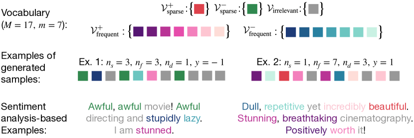
Figure 1: Visualization of the synthetic data generation process (see Section 4 for details). For simplicity, we represent each $\displaystyle d$-dimensional token with a square. Middle row: In each case, given a label $\displaystyle y$, we randomly sample $\displaystyle T=11$ tokens, with $\displaystyle n_{s}$ tokens from $\displaystyle\mathcal{V}_{\text{sparse}}^{y}$, $\displaystyle\left\lfloor(n_{f}+n_{d})/2\right\rfloor$ tokens from $\displaystyle\mathcal{V}_{\text{frequent}}^{y}$, $\displaystyle n_{f}\!-\!\left\lfloor(n_{f}+n_{d})/2\right\rfloor$ tokens from $\displaystyle\mathcal{V}_{\text{frequent}}^{-y}$ and the remaining tokens from $\displaystyle\mathcal{V}_{\text{irrelevant}}$. Note that in the first example, since $\displaystyle n_{s}\!=\!3$ and $\displaystyle n_{d}\!=\!1$, a predictor that relies (only) on the sparse tokens is less sensitive compared to the one that relies on the frequent tokens. On the other hand, in the second example, since $\displaystyle n_{s}\!=\!1$ and $\displaystyle n_{d}\!=\!3$, the predictor that relies on the frequent tokens is less sensitive. Bottom row: We include two sentiment analysis-based examples to illustrate the synthetic data samples in the second row, using the same colors as the first two rows.

$\displaystyle(n_{s},n_{f},n_{d},m)$	Using sparse tokens	Using frequent tokens
$\displaystyle(3,5,1,16)$; Fig. 2 left col.	$\displaystyle 0$	$\displaystyle 0.2878$
$\displaystyle(1,17,7,20)$; Fig. 2 right col.	$\displaystyle 0.0339$	$\displaystyle 0$

Table 1: Comparison of sensitivity values for models that use only sparse or frequent tokens for the settings considered in Figure 2.

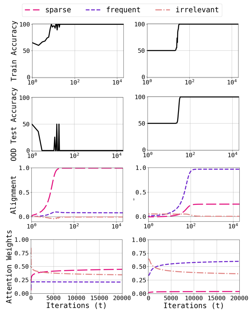
Figure 2: Train and test dynamics for a single-layer self-attention model (Eq. 3) using the synthetic data visualized in Fig. 2; see Section 4 for details. Left column: the predictor that uses sparse tokens has lower sensitivity (Ex. 1 in Figure 2), Right column: the predictor that uses frequent tokens has lower sensitivity (Ex. 2 in Figure 2); see Section A.1 for more examples.

Next, we describe the process to generate the dataset. We first define the vocabulary as follows:

Definition 4.1 (Synthetic Vocabulary).

Consider a vocabulary of $\displaystyle M$ distinct tokens $\displaystyle\mathcal{V}:=\{\bm{e}_{1},\dots\bm{e}_{M}\}$, where $\displaystyle\bm{e}_{i}\in\{0,1\}^{d}$ denotes the $\displaystyle i^{\text{th}}$ basis vector for $\displaystyle i\in[d]$. We consider smaller subsets of sparse tokens and larger subsets of frequent tokens for each label $\displaystyle y=\pm 1$, as well as a subset of irrelevant tokens, as follows:

$$\displaystyle\mathcal{V}_{\text{sparse}}^{+}:=\{\bm{e}_{1}\},\mathcal{V}_{\text{frequent}}^{+}:=\{\bm{e}_{3},\bm{e}_{5},\dots,\bm{e}_{2m+1}\},$$

$$\displaystyle\mathcal{V}_{\text{sparse}}^{-}:=\{\bm{e}_{2}\},\mathcal{V}_{\text{frequent}}^{-}:=\{\bm{e}_{4},\bm{e}_{6},\dots,\bm{e}_{2m+2}\},$$

$$\displaystyle\mathcal{V}_{\text{irrelevant}}:=\{\bm{e}_{2m+3},\dots,\bm{e}_{M}\}.$$

We now introduce some hyperparameters. Let $\displaystyle T$ represent the sequence length of each data point. Let $\displaystyle n_{f}$ and $\displaystyle n_{s}$ denote the number of frequent and sparse tokens, respectively, such that $\displaystyle n_{s}<n_{f}<\min(m,T-n_{s})$. Let $\displaystyle n_{d}$ denote a parameter satisfying $\displaystyle n_{d}\leq n_{f}$. Next, we describe the process of generating samples for the (training) dataset $\displaystyle\mathcal{D}$; see Fig. 2 for an example.

Definition 4.2 (Dataset Generation).

Consider the vocabulary in Definition 4.1. To generate a data point $\displaystyle({\bm{X}},y)$, we first sample the label $\displaystyle y\in\{\pm 1\}$ uniformly at random. We divide the indices $\displaystyle[T]$ into three sets $\displaystyle\mathcal{I}_{\text{frequent}},\mathcal{I}_{\text{sparse}}$ and $\displaystyle\mathcal{I}_{\text{irrelevant}}$, and sample each set as follows:

• $\displaystyle\mathcal{I}_{\text{frequent}}$ is composed of $\displaystyle\left\lfloor(n_{f}+n_{d})/2\right\rfloor$ tokens uniformly sampled from $\displaystyle\mathcal{V}_{\text{frequent}}^{y}$ and $\displaystyle n_{f}-\left\lfloor(n_{f}+n_{d})/2\right\rfloor$ tokens uniformly sampled from $\displaystyle\mathcal{V}_{\text{frequent}}^{-y}$.

• $\displaystyle\mathcal{I}_{\text{sparse}}$ contains $\displaystyle n_{s}$ tokens uniformly sampled from $\displaystyle\mathcal{V}_{\text{sparse}}^{y}$.

• The remaining $\displaystyle T-n_{f}-n_{s}$ tokens in $\displaystyle\mathcal{I}_{\text{irrelevant}}$ are uniformly sampled from $\displaystyle\mathcal{V}_{\text{irrelevant}}$.

To determine if the tokens in $\displaystyle\mathcal{V}_{\text{sparse}}$ or those in $\displaystyle\mathcal{V}_{\text{frequent}}$ have a more significant impact on the predictions, we adapt the test set generation process by altering the second step in Definition 4.2: we sample the sparse tokens from $\displaystyle\mathcal{V}_{\text{sparse}}^{-y}$ instead of $\displaystyle\mathcal{V}_{\text{sparse}}^{y}$. If this modification leads to a noticeable change in prediction accuracy on the test set, it suggests that the model relies on the sparse feature(s) for its predictions.

We consider two other metrics to see what tokens the model relies on and observe the role of the attention head and the linear predictor. We define three vectors,

$$\displaystyle\bm{v}_{\text{sp}}:=\bm{e}_{1}\!-\!\bm{e}_{3},\,\bm{v}_{\text{freq}}:=\!\!\!\!\!\textstyle\sum\limits_{i\in\mathcal{V}_{\text{frequent}}^{+}}\!\!\!\!\!\bm{e}_{i}-\!\!\!\!\!\!\textstyle\sum\limits_{i\in\mathcal{V}_{\text{frequent}}^{-}}\!\!\!\!\!\bm{e}_{i},\,\bm{v}_{\text{irrel}}:=\!\!\!\!\!\textstyle\sum\limits_{i\in\mathcal{V}_{\text{irrelevant}}}\!\!\!\!\!\bm{e}_{i}.$$

We plot the average alignment (cosine similarity) between the rows of $\displaystyle\bm{U}\bm{W}_{V}^{\top}$ and these vectors to see what tokens the prediction head relies on. Similarly, we plot the sum of the softmax scores for the three types of tokens to see which tokens are selected by the attention mechanism.

Finally, we define the sensitivity metric we use for high-dimensional data, which is an analog of Eq. 1.

Definition 4.3.

Given a model $\displaystyle\Phi$, dataset $\displaystyle\mathcal{D}$ and distribution $\displaystyle\mathcal{P}$, sensitivity is computed as:

$$\displaystyle\overline{S}(\Phi)=\frac{1}{T}~{}\underset{\begin{subarray}{c}{\bm{X}}\sim\mathcal{D}\\ \bm{x}\sim\mathcal{P}\end{subarray}}{\mathbb{E}}\left[\sum\limits_{\tau=1}^{T}\mathds{1}[\textsc{sign}(\Phi({\bm{\theta}};{\bm{X}}))\neq\textsc{sign}(\Phi({\bm{\theta}};{\bm{X}}^{\oplus\tau}))]\right],$$

where $\displaystyle{\bm{X}}^{\oplus\tau}$ is obtained by replacing the $\displaystyle\tau^{\text{th}}$ token in $\displaystyle{\bm{X}}$ with $\displaystyle\bm{x}$.

We set $\displaystyle\mathcal{P}$ to be the uniform distribution over $\displaystyle\mathcal{V}$ (Definition 4.1) for computing sensitivity in our experiments.

Results.

Figure 2 shows the train and test dynamics of the model in Eq. 3 using synthetic datasets generated by following the process in Definition 4.2 (details in Table 1). We consider two cases: in the first case (left column), using the sparse token leads to a function with lower sensitivity, whereas in the second case (right column), using the frequent tokens leads to lower sensitivity (see Table 1 for a comparison of the sensitivity values). We observe that in the first case, the OOD test accuracy drops to $\displaystyle 0$, the alignment with $\displaystyle\bm{v}_{\text{sp}}$ is close to $\displaystyle 1$ and the attention weights on the sparse tokens are the highest. These results show that the model relies on the sparse token in this case. On the other hand, in the second case, the test accuracy remains high, the alignment with $\displaystyle\bm{v}_{\text{freq}}$ is close to $\displaystyle 1$ and the attention weights on the frequent tokens are the highest, which shows that the model relies on the frequent tokens. These results show that the model exhibits a low-sensitivity bias. Note that in both cases, the model can learn a function that relies on a sparse set of inputs (using the sparse tokens), however, it uses these tokens only when doing so leads to lower sensitivity.

5 Experiments on Vision Tasks

In this section, we extend the experiments in the previous section to vision settings. For transformers, we consider Vision Transformers (ViT, Dosovitskiy et al.,, 2021) which obtain state-of-the-art results in computer vision tasks, and regard images as a sequence of patches (see Definition 5.1) instead of a tensor of pixels.

Definition 5.1 (Tokenization for Vision Transformers).

Let $\displaystyle\bm{X}\in\mathbb{R}^{n_{h}\times n_{w}\times n_{c}}$ be the image with height $\displaystyle n_{h}$, width $\displaystyle n_{w}$, and number of channels $\displaystyle n_{c}$. A tokenization of $\displaystyle\bm{X}$ is a sequence of $\displaystyle T$ image patches $\displaystyle\{\bm{e}_{1},\cdots,\bm{e}_{T}\}$ where each token $\displaystyle\bm{e}_{i}$ represents an image patch (see Figure 3 for an illustration of patching) of dimension $\displaystyle d=T^{-1}n_{w}n_{h}n_{c}$.

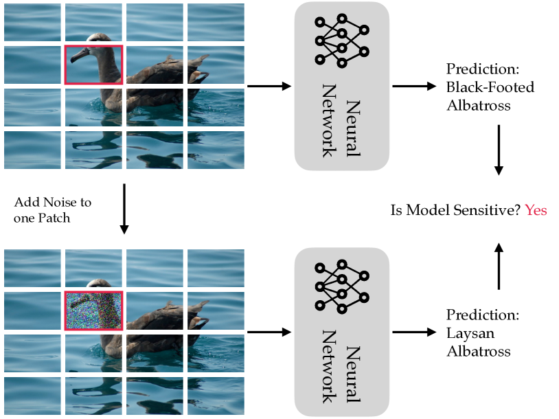
Figure 3: Measuring Sensitivity in Vision Tasks. A patch is first selected to add Gaussian noise corruptions. Then the original image and the corrupted image are fed into the same neural network to make predictions. If the predictions are inconsistent, then the neural network is sensitive to this patch. The process is repeated for every patch to measure the overall sensitivity.

Measuring Sensitivity on Images.

In our previous theory and experiments, we replaced a token with a uniformly random token to measure sensitivity. For input spaces such as natural images, there is more structure in the patches, and a uniformly random patch can fall far outside the original patch’s neighborhood. Therefore, to measure sensitivity we inject noise into the original patch instead of replacing it with a uniformly random patch. This also allows us to control the level of corruption by choosing the noise level. The measurement is illustrated in Figure 3, and we now describe it more formally. For each patch $\displaystyle\bm{e}_{j}$ of each image $\displaystyle\bm{x}$, we construct a corrupted patch $\displaystyle\bm{e}_{j}^{\prime}:=\bm{e}_{j}+\bm{\xi}_{j}$ where $\displaystyle\bm{\xi}_{j}\sim\mathcal{N}(\bm{0},\sigma^{2}\bm{I})$ is an isotropic Gaussian with variance $\displaystyle\sigma^{2}$. We measure sensitivity by replacing $\displaystyle\bm{e}_{j}$ with $\displaystyle\bm{e}_{j}^{\prime}$ as stated in Definition 4.3, with $\displaystyle\mathcal{P}$ as $\displaystyle\mathcal{N}(\bm{0},\sigma^{2}\bm{I})$. We estimate the expectation over $\displaystyle{\mathcal{P}}$ by replacing every patch with a noisy patch $\displaystyle 5$ times.

Similar to Bhattamishra et al., 2023b , sensitivity is measured on the training set. This is because our goal is to understand the simplicity bias of the model at training time, to see if it prefers to learn certain simple classes of functions on the training data. Since different models could have different generalization capabilities, the sensitivity on test data might not reflect the model’s preference for low-sensitivity functions at training time. Further, since the choice of optimization algorithm could in principle introduce its own bias and our goal is to understand the bias of the architecture, we train both the models with the same optimization algorithm, namely SGD.

We consider three datasets in this section.

Fashion-MNIST. Fashion-MNIST (Xiao et al.,, 2017) consists of $\displaystyle 28\times 28$ grayscale images of Zalando’s articles. This is a $\displaystyle 10$-class classification task with $\displaystyle 60k$ training and $\displaystyle 10k$ test images.

CIFAR-10. The CIFAR-10 dataset (Krizhevsky,, 2009) is a well-known object recognition dataset. It consists of $\displaystyle 32\times 32$ color images in $\displaystyle 10$ classes, with $\displaystyle 6k$ images per class. There are $\displaystyle 50k$ training and $\displaystyle 10k$ test images.

SVHN. Street View House Numbers (SVHN) (Netzer et al.,, 2011) is a real-world image dataset used as a digit classification benchmark. It contains $\displaystyle 32\times 32$ RGB images of printed digits ($\displaystyle 0$ to $\displaystyle 9$) cropped from Google Street View images of house number plates. There are $\displaystyle 60k$ images in the train set and $\displaystyle 10k$ images in the test set.

We compare the sensitivity of the ViT with MLPs and a CNN (LeCun et al.,, 1989) on the Fashion-MNIST dataset using $\displaystyle\sigma^{2}\!=\!5$, and with a CNN on the CIFAR-10 and the SVHN datasets using $\displaystyle\sigma^{2}\!=\!1$. We use a variant of the ViT architecture for small-scale datasets proposed in (Lee et al.,, 2021), referred to as ViT-small here onwards; see Appendix D for more details and Section A.2 for additional results for different values of depth and number of headswhere we show that varying model depths and number of heads does not affect sensitivity of ViT models.

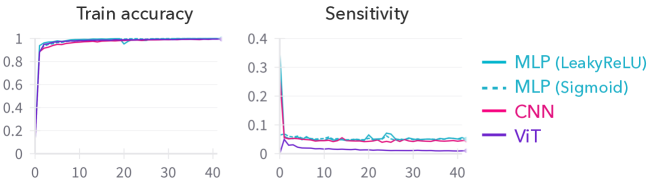
Figure 4: Sensitivity on Fashion-MNIST. Comparison of sensitivity of a ViT with a CNN, an MLP with LeakyReLU activation and an MLP with sigmoid activation, as a function of training epochs. All the models have similar accuracies but the ViT has significantly lower sensitivity.

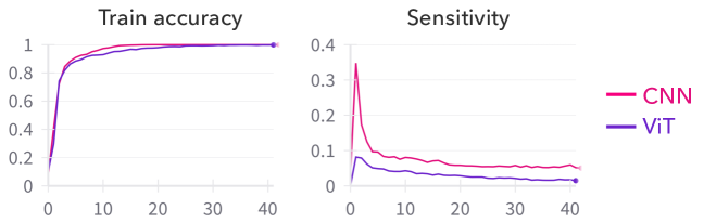
Figure 5: Sensitivity on SVHN. Comparison of sensitivity of a ResNet-18 CNN and a ViT-small trained on SVHN dataset, as a function of training epochs. Both the models have similar accuracies but the ViT has significantly lower sensitivity.

Transformers learn lower sensitivity functions than MLPs.

Figure 5 shows the training accuracy and the sensitivity of a transformer (ViT-small), a 3-hidden-layer CNN, an MLP with LeakyReLU activation and an MLP with sigmoid activation. Note that the train dynamics match closely for all the architectures, which allows for a fair comparison of sensitivity. We observe that the ViT has a lower sensitivity compared to all the other models. At the end of training, the sensitivity values are $\displaystyle 0.0559$ for the MLP with LeakyReLU, $\displaystyle 0.0505$ for the MLP with sigmoid, $\displaystyle 0.0453$ for the CNN and $\displaystyle 0.0098$ for the ViT.

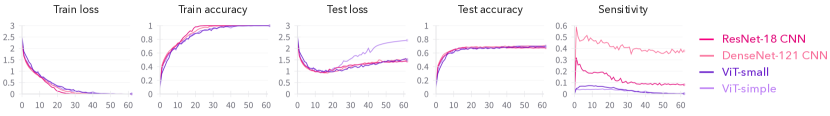
Figure 6: Sensitivity on CIFAR-10. Comparison of the sensitivity of two CNNs and two ViTs trained on the CIFAR-10 dataset, as a function of training epochs. For a fair comparison, the figure also shows the train and test accuracies and loss values (cross-entropy loss). We observe that all models have similar accuracies but the ViTs have significantly lower sensitivity than the CNNs.

Transformers learn lower sensitivity functions than CNNs.

Figure 6 shows the train and test dynamics as well as the sensitivity comparison between two ViTs: the ViT-small model used in previous experiments a ViT-simple model (Beyer et al.,, 2022), and two CNNs: a ResNet-18 (He et al.,, 2016) and a DenseNet-121 (Huang et al.,, 2016). Note that the train and test dynamics match closely for all architectures. We observe that the ViTs have a significantly lower sensitivity compared to the CNNs. At the end of training, the sensitivity values are $\displaystyle 0.3673$ for DenseNet-121, $\displaystyle 0.0827$ for ResNet-18, $\displaystyle 0.0050$ for ViT-small and $\displaystyle 0.0014$ for ViT-simple.

In Figure 5, we compare the sensitivity of the ViT-small model and the ResNet-18 on the SVHN dataset. Similar to the observations for the CIFAR-10 dataset, we see that the ViT has a significantly lower sensitivity. At the end of training, the sensitivity values are: $\displaystyle 0.0516$ for ResNet-18 and $\displaystyle 0.0147$ for ViT-small.

Based on the observations in Figures 5, 6 and 5, transformers learn lower sensitivity functions compared to other models like MLPs and CNNs.

6 Experiments on Language Tasks

In this section, we investigate the sensitivity of transformers on natural language tasks, where each datapoint is a sequence of sparse tokens. Similar to the comparison of Vision Transformers with MLPs and CNNs in Section 5, we compare a RoBERTa (Liu et al.,, 2019) transformer model with LSTMs (Hochreiter and Schmidhuber,, 1997), an alternative auto-regressive model, in this section. Recall that we consider a transformer with linear attention for the results in Section 3. Aligning with this setup, we also consider a RoBERTa model with ReLU activation in the attention layer (i.e., replacing $\displaystyle\bm{\varphi}(\cdot)$ in Eq. 3 with $\displaystyle\mathrm{ReLU}(\cdot)$) for our experiments.

We use the sameusual RoBERTa-like tokenization procedure to process inputs for all the models so that they are represented as <s> $\displaystyle e_{1},\cdots,e_{T}$ </s> where each $\displaystyle e_{j}$ represents tokens that are usually subwords and <s> represents the classification (CLS) token, $\displaystyle T$ the sequence length, and </s> the separator token. We denote $\displaystyle e_{0}=$<s> and $\displaystyle e_{-1}=e_{T+1}=$ </s>. For each token $\displaystyle e_{j}$, a token embedding $\displaystyle h_{E}(\cdot):[M]\rightarrow\mathbb{R}^{d}$ is trained during the process, where $\displaystyle M$ denotes the vocabulary size. For transformers, we also train a separate positional encoder $\displaystyle h_{P}(\cdot):[N]\rightarrow\mathbb{R}^{d}$, where $\displaystyle N$ denotes the maximum sequence length. We denote $\displaystyle\bm{e}_{j}^{\text{\tiny{LSTM}}}=h_{E}^{\text{\tiny{LSTM}}}(e_{j})$ as the embedded token of LSTM and $\displaystyle\bm{e}_{j}^{\text{\tiny{RoBERTa}}}=h_{E}^{\text{\tiny{RoBERTa}}}(e_{j})+h_{P}^{\text{\tiny{RoBERTa}}}(j)$ as the embedding token of RoBERTa. For convenience, we omit the superscript and denote these learned embeddings as $\displaystyle\bm{e}_{j}$.

Measuring Sensitivity on Language.

We adopt the same approach to measure sensitivity as in Section 5 for the vision tasks. Specifically, we add Gaussian noise $\displaystyle\bm{\xi}_{j}\sim\mathcal{N}(\bm{0},\sigma^{2}\bm{I})$ to token embedding $\displaystyle\bm{e}_{j}$ to generate a corrupted embedding $\displaystyle\bm{e}_{j}^{\prime}=\bm{e}_{j}+\bm{\xi}_{j}$ and measure sensitivity by replacing $\displaystyle\bm{e}_{j}$ with $\displaystyle\bm{e}_{j}^{\prime}$, as stated in Definition 4.3. We note that to control the relative magnitude of noise, the embeddings $\displaystyle\bm{e}_{j}\leftarrow\texttt{LayerNorm}(\bm{e}_{j})$ are first layer-normalized (Ba et al.,, 2016) before the additive Gaussian corruption, for both the models.

In order to better control possible confounders, we limit both LSTM and RoBERTa to having the same number of layers and heads. We choose $\displaystyle 4$ layers and $\displaystyle 8$ heads at each layer, to achieve reasonable performance. Both models are trained from scratch, without any pretraining on larger corpora, to ensure fair comparisons.

We consider the following two binary classification datasets, which are relatively easy to learn without pretraining (Kovaleva et al.,, 2019).

MRPC. Microsoft Research Paraphrase Corpus (MRPC, Dolan and Brockett,, 2005) is a corpus that consists of $\displaystyle 5801$ sentence pairs. Each pair is labeled if it is a paraphrase or not by human annotators. It has $\displaystyle 4076$ training examples and $\displaystyle 1725$ validation examples.

QQP. Quora Question Pairs (QQP, Iyer et al.,, 2017) dataset is a corpus that consists of over $\displaystyle 400k$ question pairs. Each question pair is annotated with a binary value indicating whether the two questions are paraphrases of each other. It has $\displaystyle 364k$ training examples and $\displaystyle 40k$ validation examples.

Empirically, we choose the variance $\displaystyle\sigma^{2}=15$ (consistent with Bhattamishra et al., 2023b, ); we include results with $\displaystyle\sigma^{2}=4$ in Section A.3, which yield similar observations. Similar to Section 5, we measure sensitivity on the train set; we include results on the validation set in Section A.3 and they yield similar observations. Section A.3 also contains further results with a GPT-2 architecture, and different choices for the depth of the model. We observe similar conclusions with these variations as the results presented in this section.

Transformers learn lower sensitivity functions than LSTMs.

As shown in LABEL:fig:nlp-sensitivity, both RoBERTa models have lower sensitivity than LSTMs on both datasets, regardless of the number of datapoints trained. Even at initialization with random weights, LSTMs are more sensitive. At the end of training, the sensitivity values on the MRPC dataset are $\displaystyle 0.15$, $\displaystyle 0.002$ and $\displaystyle 0.001$ for the LSTM, the RoBERTa model with softmax activation and the RoBERTa with ReLU activation, respectively. On the QQP dataset, LSTM, RoBERTa-softmax and RoBERTa-ReLU have sensitivity values of $\displaystyle 0.09$, $\displaystyle 0.03$ and $\displaystyle 0.02$, respectively. Interestingly, RoBERTa with ReLU activation also has lower sensitivity than its softmax counterparts. This may be because softmax attention encourages sparsity because of which the model can be more sensitive to a particular token; see Ex. 2 in Figure 2 and bottom row of Figure 2 for an example where sparsity can lead to higher sensitivity.

LSTMs are more sensitive to later tokens.

In LABEL:fig:nlp-sensitivity-position, we plot sensitivity over the token positions. We observe that LSTMs exhibit larger sensitivity towards the end of the sequence, i.e. at later token positions. In contrast, transformers are relatively uniform. Similar observations were made by Fu et al., (2023) for a linear regression setting, where they found that LSTMs do more local updates and only remember the most recent observations, whereas transformers preserve global information and have longer memory.

Transformers are sensitive to the CLS token.

In LABEL:fig:nlp-sensitivity-position, we also observe that the RoBERTa model with softmax activation has frequent bumps in the sensitivity values at early token positions. This is because different sequences have different lengths and while computing sensitivity versus token positions, we align all the sequences to the right. These bumps at early token positions indeed correspond to the starting token after the tokenization procedure, the CLS token <s>. This aligns with the observations of Jawahar et al., (2019) that the CLS token gathers all global information. Perturbing the CLS token corrupts the aggregation and results in high sensitivity.

7 Implications of the Low Sensitivity Bias

We saw in Section 5 that transformers learn lower sensitivity functions than CNNs. In this section, we first compare the test performance of these models on the CIFAR-10-C dataset and show that transformers are more robust than CNNs. Next, we add a regularization term while training the transformer, to encourage lower sensitivity. The results imply that lower sensitivity leads to improved robustness. Additionally, we explore the connection between sensitivity and the flatness of the minima. Our results imply that lower sensitivity leads to flatter minima.

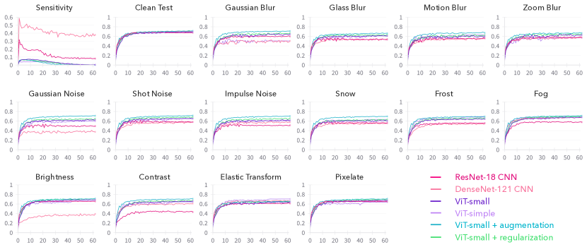
Figure 11: Lower sensitivity leads to better robustness. Comparison of the sensitivity, test accuracy on CIFAR-10 and test accuracies on various corruptions from blur, noise, weather and digital categories from the CIFAR-10-C dataset (see Section 7 for details) of two CNNs and two ViTs trained on the CIFAR-10 dataset, as a function of the training epochs. We also compare with ViT-small trained with data augmentation/regularization, which encourage low sensitivity (see Section 7 for discussion).

7.1 Lower Sensitivity leads to Improved Robustness

The CIFAR-10-C dataset (Hendrycks and Dietterich,, 2019) was developed to benchmark the performance of various NNs on object recognition tasks under common corruptions which are not confusing to humans. Images from the test set of CIFAR-10 are corrupted with $\displaystyle 14$ types of algorithmically generated corruptions from blur (Gaussian, glass, motion, zoom), noise (Gaussian, shot, impulse), weather (snow, frost, fog), and digital (brightness, contrast, elastic transform, pixelate) categories (see Fig. 1 in Hendrycks and Dietterich, (2019) for examples). There are $\displaystyle 5$ severity levels (see Fig. 7 in the Appendix of Hendrycks and Dietterich, (2019) for an example) and we use severity level $\displaystyle 2$ for our experiments. We also include results on severity level $\displaystyle 1$ in Section A.2.

Figure 11 compares the performance of two CNNs: ResNet-18 and DenseNet-121 with two ViTs: ViT-small and ViT-simple on various corruptions from the CIFAR-10-C dataset. We observe that the ViTs have lower sensitivity and better test performance on almost all corruptions compared to the CNNs, which have a higher sensitivity; see Section A.2 for a comparison at the end of training. Since the definition of sensitivity involves the addition of noise and ViTs have lower sensitivity, one can expect the ViTs to perform better on images with various noise corruptions. However, perhaps surprisingly, the ViTs also have better test performance on several corruptions from weather and digital categories, which are significantly different from noise corruptions.

Next, we conduct an experiment to investigate the role of low sensitivity in the robustness of transformers. We add a regularization term while training the model to explicitly encourage it to have lower sensitivity. If this model is more robust, then we can disentangle the role of low sensitivity from the role of the architecture and establish a causal connection between lower sensitivity and improved robustness. To add the regularization, we use the fact that sensitivity can be estimated efficiently via sampling and consider two methods. In the first method (augmentation), we augment the training set by injecting the images with Gaussian noise (mean $\displaystyle 0$, variance $\displaystyle 0.1$) while preserving the label, and train the ViT on the augmented training set. In the second method (regularization), we add a mean squared error term for the model outputs for the original image and the image with Gaussian noise (mean $\displaystyle 0$, variance $\displaystyle 1$) injected into a randomly selected patch. We use a regularization strength of $\displaystyle 0.25$.

Figure 11 also shows the test performance of ViT-small trained with augmentation and regularization methods on various corruptions from the CIFAR-10-C dataset. We observe that the ViTs trained with these methods exhibit lower sensitivity compared to vanilla training. This is accompanied by an improved test performance on various corruptions, particularly on corrupted images from the noise and blur categories. Together, these results indicate that the simplicity bias of transformers to learn functions of lower sensitivity leads to improved robustness (to common corruptions) compared to CNNs.

We note that Hendrycks and Dietterich, (2019) show that methods that improve robustness to corruptions also improve robustness to perturbations. Consequently, these results also suggest why transformers are more robust to adversarial perturbations compared to CNNs (Mahmood et al.,, 2021; Shao et al.,, 2021).

7.2 Lower Sensitivity leads to Flatter Minima

In this section, we investigate the connection between low sensitivity and flat minima. Consider a linear model $\displaystyle\Phi({\bm{\theta}};\bm{x})={\bm{\theta}}^{\top}\bm{x}$. Measuring sensitivity involves perturbing the input vector $\displaystyle\bm{x}$ by some $\displaystyle\Delta\bm{x}$. Computing the perturbed prediction $\displaystyle\Phi({\bm{\theta}};\bm{x}+\Delta\bm{x})$ is equivalent to perturbing the weight vector $\displaystyle{\bm{\theta}}$ with $\displaystyle\Delta{\bm{\theta}}=\tfrac{{\bm{\theta}}^{\top}\Delta\bm{x}}{\|\bm{x}\|_{2}^{2}}\bm{x}$, as

$$\displaystyle\Phi({\bm{\theta}};\bm{x}+\Delta\bm{x})={\bm{\theta}}^{\top}(\bm{x}+\Delta\bm{x})=\Phi({\bm{\theta}};\bm{x})+{\bm{\theta}}^{\top}\Delta\bm{x}=\Phi({\bm{\theta}};\bm{x})+\Delta{\bm{\theta}}^{\top}\bm{x}=\Phi({\bm{\theta}}+\Delta{\bm{\theta}};\bm{x}).$$

This draws a natural connection between sensitivity, which is measured with perturbation in the input space, and flatness of minima, which is measured with perturbation in the weight space (Keskar et al.,, 2017). Below, we investigate whether such a connection extends to more complex architectures such as transformers.

Setting		ShOp		ShPred
ViT-small + vanilla training		$\displaystyle 39.166$		$\displaystyle 0.5346$
ViT-small + sensitivity regularization		$\displaystyle 9.025$		$\displaystyle 0.3982$

Table 2: Comparison of two sharpness metrics at the end of training the ViT-small model on the CIFAR-10 dataset with and without the sensitivity regularization. Lower values correspond to flatter minima; see text for discussion.

In Table 2, we compare the flatness of the minima for the ViT-small model trained with and without the sensitivity regularization at the end of training. Specifically, given model $\displaystyle\Phi$, we consider the following two metrics, based on the model outputs and model predictions, respectively,

ShOp $$\displaystyle:=\mathbb{E}_{\bm{x}\sim\mathcal{D},\bm{\xi}\sim{\mathcal{N}}(0,\sigma^{2}\bm{I})}|\Phi({\bm{\theta}};\bm{x})-\Phi({\bm{\theta}}+\bm{\xi};\bm{x})|,$$

ShPred $$\displaystyle:=\mathbb{E}_{\bm{x}\sim\mathcal{D},\bm{\xi}\sim{\mathcal{N}}(0,\sigma^{2}\bm{I})}\mathds{1}[f({\bm{\theta}};\bm{x})\neq f({\bm{\theta}}+\bm{\xi};\bm{x})],$$

where $\displaystyle f({\bm{\theta}};\bm{x})=\mathds{1}[\Phi({\bm{\theta}};\bm{x})\geq 0]$ and $\displaystyle\mathcal{D}$ denotes the train set. Intuitively, for a flatter minima, the model output and hence its prediction would remain relatively invariant to small perturbations in the model parameters.

We find that both metrics indicate that lower sensitivity corresponds to a flatter minimum. It is widely believed that flatter minima correlate with better generalization (Jiang* et al.,, 2020; Keskar et al.,, 2017; Neyshabur et al.,, 2017). However, recent work (Andriushchenko et al.,, 2023) has suggested that these may not always be correlated. Our results indicate that low-sensitivity correlates with improved generalization and investigating this connection for other settings can be an interesting direction for future work.

8 Discussion

Our results demonstrate that sensitivity is a promising notion to understand the simplicity bias of transformers and suggest several directions for future work. On the theoretical side, though our results show that transformers have a spectral bias, they leave open the question of how their bias compares with other architectures. Given our empirical findings, a natural theoretical direction is to show that transformers have a stronger spectral bias than other architectures. On the empirical side, it would be interesting to further explore the connections between sensitivity and robustness, particularly as it relates to out-of-distribution (OOD) robustness and dependence on spurious features. It seems conceivable that transformers’ preference towards a rich set of features (such as in the synthetic experiment in Section 4) helps the model avoid excessive reliance on spurious features in the data and hence promotes robustness. Understanding and developing this connection could explain the improved OOD robustness of transformers.

Appendix

[appendix]

[appendix]1

Appendix A Additional Experiments

In this section, we include some additional results to supplement the main experimental results for synthetic data as well as the vision and language tasks.

A.1 Synthetic Data and the MNIST Dataset

In this section, we present some additional results for the low-sensitivity bias of a single-layer self-attention model (Eq. 3) on the synthetic dataset generated based on Definition 4.2, visualized in Fig. 2. Similar to the results in Section 4, we consider three data settings where using the sparse token leads to a function with lower sensitivity (Fig. 12, top row) and three settings where using the frequent token leads to lower sensitivity (Fig. 12, bottom row). The exact data settings and a comparison of the sensitivity values for each setting are shown in Table 3. These results yield similar conclusions as in Section 4: in both cases, the model uses tokens which leads to a lower sensitivity function.

	Top row in Fig. 2 $\displaystyle(n_{s}=3,n_{d}=1)$			Bottom row in Fig. 2 $\displaystyle(n_{s}=1,n_{d}=7)$
Data Setting $\displaystyle(n_{f},m)$	$\displaystyle(3,6)$	$\displaystyle(5,16)$	$\displaystyle(7,28)$	$\displaystyle(7,10)$	$\displaystyle(17,20)$	$\displaystyle(32,36)$
Using sparse tokens	$\displaystyle 0$	$\displaystyle 0$	$\displaystyle 0$	$\displaystyle 0.0339$	$\displaystyle 0.0339$	$\displaystyle 0.0339$
Using frequent tokens	$\displaystyle 0.1315$	$\displaystyle 0.2878$	$\displaystyle 0.4502$	$\displaystyle 0$	$\displaystyle 0$	$\displaystyle 0$

Table 3: Comparison of sensitivity values for models that use only sparse or frequent tokens for the settings considered in Fig. 12.

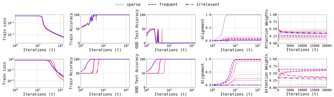
Figure 12: Train and test dynamics for a single-layer self-attention model (Eq. 3) using the synthetic data visualized in Fig. 2; see Section 4 for details. The top row corresponds to the cases where the predictor that uses sparse tokens has lower sensitivity, while the bottom row corresponds to the cases where using the frequent tokens leads to lower sensitivity. The precise data settings for this figure, as well as a comparison of sensitivity values, are shown in Table 3.

Continuing from the synthetic data, we now consider a slightly more complicated dataset, namely MNIST (LeCun and Cortes,, 2005). The MNIST dataset consists of $\displaystyle 70k$ black-and-white images of handwritten digits of resolution $\displaystyle 28\times 28$. There are $\displaystyle 60k$ images in the training set and $\displaystyle 10k$ images in the test set. We compare the sensitivity of a ViT-small model with an MLP on a binary digit classification task ($\displaystyle<5$ or $\displaystyle\geq 5$). In our experiments, each image is divided into $\displaystyle T=16$ patches of size $\displaystyle 7\times 7$ for the ViT-small model. For the MLP, the inputs are vectorized as usual. With this setting, we measure the sensitivity of the two models using patch token replacement as per Definition 4.3. As shown in Figure 14, when achieving the same training accuracy, the ViT shows lower sensitivity compared to the MLP.

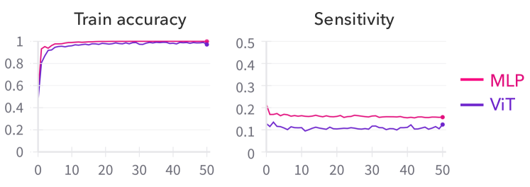
Figure 13: Sensitivity on MNIST. ViT and MLP get similar accuracy, but the ViT has lower sensitivity.

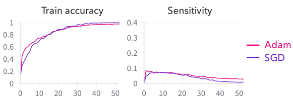
Figure 14: Sensitivity using SGD and Adam. Comparison of train accuracies and sensitivity values of the ViT-small model trained on the CIFAR-10 dataset using SGD and Adam optimizers.

A.2 Vision Tasks

Effect of Depth, Number of Heads and the Optimization Algorithm.

In Fig. 14, we compare the sensitivity values of a ViT-small model trained on CIFAR-10 dataset with SGD and Adam optimization algorithms. Although the model trained with Adam has a slightly higher sensitivity, the sensitivity values for both the models are quite similar. This indicates that the low-sensitivity bias is quite robust to the choice of the optimization algorithm.

In LABEL:fig:sens-depth-heads, we compare the sensitivity values of a ViT-small model with different depth and number of attention heads, when trained on the CIFAR-10 dataset. Note that for our main results, we use a model with depth $\displaystyle 8$ and $\displaystyle 32$ heads. We observe that the train accuracies and the sensitivity values remain the same across the different model settings. This indicates that the low-sensitivity bias is quite robust to the model setting.

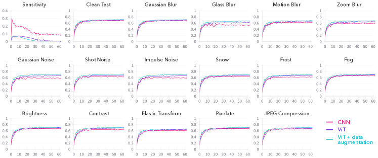
Figure 16: Comparison of the sensitivity, test accuracy on CIFAR-10 and test accuracies on various corruptions from blur, noise, weather and digital categories from the CIFAR-10-C dataset (see Section 7 for details) of a ResNet-18 CNN and a ViT-small model trained on the CIFAR-10 dataset, as a function of the training epochs. We also compare with ViT-small trained with data augmentation, which acts as a regularizer to encourage low sensitivity (see Section 7 for discussion). Here, we use severity level $\displaystyle 1$, while in Figure 11, we considered severity level $\displaystyle 2$.

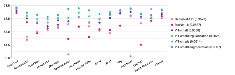
Figure 17: Comparison of the test accuracies on CIFAR-10 and on various corruptions from blur, noise, weather and digital categories from the CIFAR-10-C dataset (see Section 7 for details) of two CNNs, two ViTs and ViT-small with augmentation/regularization trained on the CIFAR-10 dataset, at the last training epoch. The legend is arranged in order of decreasing sensitivity values (included in parenthesis); see Fig. 11 for a comparison of the accuracies as a function of training epochs.

Additional Results on CIFAR-10-C.

Fig. 16 shows the test performance on CIFAR-10-C dataset with severity level $\displaystyle 1$. We observe that similar to Fig. 11, where we considered severity level $\displaystyle 2$, CNNs have lower test accuracies on corrupted images compared to ViTs. Further, encouraging lower sensitivity in the ViT leads to better robustness. However, the gains are smaller in this case due to the lower severity level.

In Fig. 17, we compare the test accuracies on CIFAR-10 as well as on various corruptions from the CIFAR-10-C dataset, at the end of training. We observe that models with lower sensitivity have higher accuracies across most corruptions.

A.3 Language Tasks

Sensitivity Measured with Variance $\displaystyle\sigma^{2}=4$.

Alternative to the main experiments with $\displaystyle\sigma^{2}=15$, we also evaluate sensitivity with a different corruption strength $\displaystyle\sigma^{2}=4$ on the QQP dataset, as shown in LABEL:fig:sensitivity_nlp_var_4. We observe the same trends as in LABEL:fig:nlp-sensitivity and LABEL:fig:nlp-sensitivity-position: RoBERTa models have lower sensitivity than the LSTM and the LSTM is more sensitive to more recent tokens. These results indicate that the low-sensitivity bias is robust to the choice of the corruption strength.

Sensitivity Measured on the Validation Set.

We also test sensitivity on the validation set for the two language datasets. As seen in LABEL:fig:sensitivity_nlp_val, the results on the validation set are consistent with those on the train set in LABEL:fig:nlp-sensitivity.

Sensitivity Measured with the GPT-2 Model.

Here, we ablate the effect of the transformer architecture on the sensitivity values. We compare a GPT-based model with the two BERT-based models used in our main experiments. The key difference lies in the construction of the attention masks: for GPT models, each token only observes the tokens that appear before it, whereas BERT models are bidirectional, therefore each token observes all the tokens in the sequence. In LABEL:fig:sensitivity_nlp_gpt, we observe that the GPT-2 model has higher sensitivity compared to the RoBERTa models, but the sensitivity is significantly lower than the LSTM. The GPT-2 model is also relatively more sensitive to more recent tokens compared to the RoBERTa models, while also being sensitive to some CLS tokens.

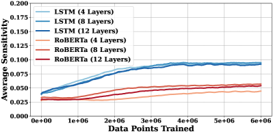
Figure 19: Sensitivity for Different Model Depths. We vary the model depths of LSTM and RoBERTa on the QQP datasets and observe that LSTM models tend to have the same sensitivity throughout the entire training. RoBERTa model with 4 layers has slightly lower sensitivity with its 8-layer or 12-layer variants. Nonetheless, RoBERTa models, regardless of depths, have lower sensitivity than LSTMs.

Appendix B Proof of Proposition 3.1

Hron et al., (2020) show that the self-attention layer (Eq. 2) with linear attention and $\displaystyle d^{-1/2}$ scaling converges in distribution to $\displaystyle\mathcal{GP}(0,K)$ in the infinite width limit, i.e. when the number of heads $\displaystyle d^{H}$ become large. For any layer $\displaystyle l\in[L]$, let $\displaystyle\tilde{K}^{l}$ denote the kernel induced by the intermediate transformation when applying some nonlinearity $\displaystyle\phi$ to the output of the previous layer $\displaystyle l-1$. Let $\displaystyle f^{l}_{\cdot j}:=\{f^{l}_{i,j}({\bm{x}}):{\bm{x}}\in\mathcal{X},i\in[T]\}$, where $\displaystyle\mathcal{X}$ denotes the input space of $\displaystyle{\bm{x}}$. They show the following result for NNs with at least one linear attention layer, in the infinite width limit.

Theorem B.1 (Theorem 3 in Hron et al., (2020)).

Let $\displaystyle l\in[L]$, and $\displaystyle\phi$ be such that $\displaystyle|\phi(x)|\leq c+m|x|$ for some $\displaystyle c,m\in\mathbb{R}^{+}$. Assume $\displaystyle g^{l-1}$ converges in distribution to $\displaystyle g^{l-1}\sim GP(0,K^{l-1})$, such that $\displaystyle g_{\cdot j}^{l-1}$ and $\displaystyle g_{\cdot k}^{l-1}$ are independent for any $\displaystyle j\neq k$. Then as $\displaystyle\min\{d^{l,H},d^{l}\}\rightarrow\infty$, $\displaystyle g^{l}$ converges in distribution to $\displaystyle g^{l}\sim GP(0,K^{l})$ with $\displaystyle g_{\cdot k}^{l}$ and $\displaystyle g_{\cdot\ell}^{l}$ independent for any $\displaystyle k\neq\ell$, and

$$\displaystyle K^{l}({\bm{x}},{\bm{x}}^{\prime})=\mathbb{E}[g^{l}({\bm{x}})g^{l}({\bm{x}}^{\prime})]=\sum\limits_{i,j=1}^{\tilde{d}}(\tilde{K}^{l}_{ij}({\bm{x}},{\bm{x}}^{\prime}))^{2}\tilde{K}^{l}_{ab}({\bm{x}},{\bm{x}}^{\prime}).$$

Similar results are also known for several non-linearities and other layers such as convolutional, dense, average pooling (Lee et al.,, 2018; de G. Matthews et al.,, 2018; Garriga-Alonso et al.,, 2019; Novak et al.,, 2019; Yang,, 2021), as well as residual, positional encoding and layer normalization (Hron et al.,, 2020; Yang,, 2021).

Consequently, any model composed of these layers, such as a transformer with linear attention, also converges to a Gaussian process. This follows using an induction-based argument. It can easily be shown that the induced kernel takes the form

$$\displaystyle K({\bm{x}},{\bm{y}})=\Psi\left(\frac{\left\langle{\bm{x}},{\bm{y}}\right\rangle}{\left\|{\bm{x}}\right\|\left\|{\bm{y}}\right\|},\frac{\left\|{\bm{x}}\right\|^{2}}{d},\frac{\left\|{\bm{y}}\right\|^{2}}{d}\right),$$

for some function $\displaystyle\Psi:\mathbb{R}^{3}\rightarrow\mathbb{R}$. In addition, since $\displaystyle{\bm{x}},{\bm{y}}\in\text{\mancube}^{d}$, they have the same norm, and $\displaystyle\Psi$ can be treated as a univariate function that only depends on $\displaystyle c=d^{-1}\left\langle{\bm{x}},{\bm{y}}\right\rangle$, i.e. $\displaystyle\Psi\left(c,1,1\right)=\Psi(c)$.

Using this property and the following result, it follows that the kernel induced by a transformer with linear attention is diagonalized by the Fourier basis $\displaystyle\{\chi_{U}\}_{U\subseteq[d]}$.

Theorem B.2 (Theorem 3.2 in Yang and Salman, (2020)).

On the $\displaystyle d$-dimensional boolean cube $\displaystyle\text{\mancube}^{d}$, for every $\displaystyle U\subseteq[d]$, $\displaystyle\chi_{U}$ is an eigenfunction of $\displaystyle K$ with eigenvalue

$$\displaystyle\mu_{|U|}:=\mathop{\mathbb{E}}_{{\bm{x}}\sim\text{\mancube}^{d}}\left[x^{U}K({\bm{x}},\mathbf{1})\right]=\mathop{\mathbb{E}}_{{\bm{x}}\sim\text{\mancube}^{d}}\left[x^{U}\Psi\left(d^{-1}\textstyle\sum\limits_{i}x_{i}\right)\right],$$

where $\displaystyle\mathbf{1}:=(1,\dots,1)\in\text{\mancube}^{d}$. This definition of $\displaystyle\mu_{|U|}$ does not depend on the choice $\displaystyle S$, only on the cardinality of $\displaystyle S$. These are all of the eigenfunctions of $\displaystyle K$ by dimensionality considerations.

Further, using the following result, it follows that transformers (with linear attention) exhibit weak spectral simplicity bias.

Theorem B.3 (Theorem 4.1 in Yang and Salman, (2020)).

Let $\displaystyle K$ be the CK or NTK of an MLP on a boolean cube $\displaystyle\text{\mancube}^{d}$. Then the eigenvalues $\displaystyle\mu_{k},k=0,\dots,d$, satisfy

$$\displaystyle\mu_{0} \displaystyle\geq\mu_{2}\geq\dots\geq\mu_{2k}\geq\dots,$$

$$\displaystyle\mu_{1} \displaystyle\geq\mu_{3}\geq\dots\geq\mu_{2k+1}\geq\dots.$$

Appendix C Further Related Work

Implicit Biases of Gradient Methods.

Several works study the implicit bias of gradient-based methods for linear predictors and MLPs. Pioneering work by Soudry et al., (2018); Ji and Telgarsky, (2018) revealed that linear models trained with gradient descent to minimize an exponentially-tailed loss on linearly separable data converge (in direction) to the max-margin classifier. Following this, Nacson et al., (2019); Ji and Telgarsky, (2021); Ji et al., (2021) derived fast convergence rates for gradient-based methods in this setting. Recent works show that MLPs trained with gradient flow/descent converge to a KKT point of the corresponding max-margin problem in the parameter space, in both finite (Ji and Telgarsky,, 2020; Lyu and Li,, 2020) and infinite width (Chizat and Bach,, 2020) regimes. Further, Phuong and Lampert, (2021); Frei et al., (2022); Kou et al., (2023) have also studied ReLU/Leaky-ReLU networks trained with gradient descent on nearly orthogonal data. Li et al., (2022) show that the training path in over-parameterized models can be interpreted as mirror descent applied to an alternative objective. In regression problems, when minimizing the mean squared error, the bias manifests in the form of rank minimization (Arora et al.,, 2019; Li et al.,, 2021). Additionally, the implicit bias of other optimization algorithms, such as stochastic gradient descent and adaptive methods, has also been explored in various studies (Blanc et al.,, 2020; HaoChen et al.,, 2021); see the recent survey Vardi, (2022) for a detailed summary.

Robustness.

Several research efforts have been made to investigate the robustness of Transformers. Shao et al., (2021) showed that Transformers exhibit greater resistance to adversarial attacks compared to other models. Additionally, Mahmood et al., (2021) highlighted the notably low transferability of adversarial examples between CNNs and ViTs. Subsequent research (Shen et al.,, 2023; Bhojanapalli et al.,, 2021; Paul and Chen,, 2022) expanded this robustness examination to improve transformer-based language models. Shi et al., (2020) introduced the concept of robustness verification in Transformers. Various robust training methods have been suggested to enhance the robustness guarantees of models, often influenced by or stemming from their respective verification techniques. Shi et al., (2021) expedited the certified robust training process through the use of interval-bound propagation. Wang et al., (2021) employed randomized smoothing to train BERT, aiming to maximize its certified robust space. Recent work (Bombari and Mondelli,, 2024) shows that randomly-initialized attention layers tend to have higher word-level sensitivity than fully connected layers. In contrast to our work, they consider word sensitivity, which has been experimentally shown to be similar for transformers and LSTMs (Bhattamishra et al., 2023b, ).

Spurious Correlations.

A common pitfall to the generalization of neural networks is the presence of spurious correlations (Sagawa et al.,, 2020). For example, Geirhos et al., (2019) observed that trained CNNs are biased towards textures rather than shapes to make predictions for object recognition tasks. Such biases make NNs vulnerable to adversarial attacks. Gururangan et al., (2018) attribute the reliance of NNs on spurious features to confounding factors in data collection while Shah et al., (2020) attribute it to a simplicity bias. Several works have studied the underlying causes of simplicity bias (Chiang,, 2021; Nagarajan et al.,, 2021; Morwani et al.,, 2023; Huh et al.,, 2021; Lyu et al.,, 2021) and multiple methods have been developed to mitigate this bias and improve generalization (Pezeshki et al.,, 2020; Kirichenko et al.,, 2022; Vasudeva et al.,, 2023; Tiwari and Shenoy,, 2023).

Data Augmentation.

The essence of data augmentation is to impose some notion of regularization. The simplest design of data augmentation dates back to Robbins, (1951) where image manipulation, e.g., flip, crop, and rotate, was introduced. Bishop, (1995) proved that training with Gaussian noise is equivalent to Tikhonov regularization. We also note this observation is in parallel to our proposition in Section 7 that training with Gaussian noise promotes low sensitivity. Recently, mixup-based augmentation methods have been proposed to improve model robustness by merging two images as well as their labels (Zhang et al.,, 2018). Several works also use a combination of existing augmentation techniques (Cubuk et al.,, 2019; Lim et al.,, 2019). A common belief is that data augmentation can improve model robustness (Rebuffi et al.,, 2021), and this work bridges the method (augmentation) and the outcome (robustness) with an explanation — simplicity bias towards low sensitivity.

Appendix D Details of Experimental Settings

Experimental Settings for Synthetic Data Experiments.

We use standard SGD training with batch size $\displaystyle 100$. We consider $\displaystyle T=50$ and train with $\displaystyle 1000$ samples and test on $\displaystyle 500$ samples generated as per Definition 4.2.

Model Architectures and Experimental Settings for Vision Tasks.

For all the datasets, we use the ViT-small architecture implementation available at https://github.com/lucidrains/vit-pytorch. For the ResNet-18 model used in the experiments on CIFAR-10 and SVHN datasets, we use the implementation available at https://github.com/kuangliu/pytorch-cifar. Additionally, for the DenseNet-121 model and ViT-simple model used in the experiments on CIFAR-10, we use the implementations available at https://github.com/huyvnphan/PyTorch_CIFAR10 and https://github.com/lucidrains/vit-pytorch, respectively. All the models are trained with SGD using batch size $\displaystyle 50$ for MNIST and $\displaystyle 100$ for the other datasets. We use patch size $\displaystyle 7$ for MNIST and $\displaystyle 4$ for the other datasets.

For the MNIST experiments, we consider a 1-hidden-layer MLP with $\displaystyle 100$ hidden units and LeakyReLU activation. We set depth as $\displaystyle 2$, number of heads as $\displaystyle 1$ and the hidden units in the MLP as $\displaystyle 128$ for the ViT. We train both models with a learning rate of $\displaystyle 0.01$.

For Fashion-MNIST, we set depth as $\displaystyle 2$, number of heads as $\displaystyle 8$ and the hidden units in the MLP as $\displaystyle 256$ for the ViT. We consider a 2-hidden layer MLP with $\displaystyle 512$ and $\displaystyle 128$ hidden units, respectively. The CNN consists of two 2D convolutional layers with $\displaystyle 32$ output channels and kernel size $\displaystyle 3$ followed by a 2D MaxPool layer with both kernel size and stride as $\displaystyle 2$ and two fully connected layers with $\displaystyle 128$ hidden units. We use LeakyReLU activation for the CNN. We use learning rates of $\displaystyle 0.1$ for the MLP with LeakyReLU, $\displaystyle 0.5$ for the MLP with sigmoid, $\displaystyle 0.005$ for the CNN and $\displaystyle 0.1$ for the ViT.

For CIFAR-10, we set depth as $\displaystyle 8$, number of heads as $\displaystyle 32$ and the hidden units in the MLP as $\displaystyle 256$ for the ViT-small model, while these values are set as $\displaystyle 6$, $\displaystyle 16$, and $\displaystyle 512$ for the ViT-simple model. The learning rate is set as $\displaystyle 0.1$ for ViT-small, $\displaystyle 0.2$ for ViT-simple, $\displaystyle 0.001$ for ResNet-18 and $\displaystyle 0.005$ for DenseNet-121.

For SVHN, most of the settings are the same as the CIFAR-10 experiments, except we set the hidden units in the MLP as $\displaystyle 512$ for the ViT-small model and the learning rate is set as $\displaystyle 0.0015$ for ResNet-18.

Model Architectures and Experimental Settings for Language Tasks.

For both RoBERTa models and LSTM models, we keep the same number of layers and number of heads: $\displaystyle 4$ layers and $\displaystyle 8$ heads each. We use the AdamW optimizer with a learning rate of $\displaystyle 0.0001$ and weight decay of $\displaystyle 0.0001$ for all the tasks. We also use a dropout rate of $\displaystyle 0.1$. We use a batch size of $\displaystyle 32$ for all the experiments.

Experimental Settings for Section 7.

We set the learning rate as $\displaystyle 0.16$ and $\displaystyle 0.2$ when training the ViT-small with regularization and augmentation, respectively. The remaining settings are the same as for the other experiments. For computing the sharpness metrics, we approximate the expectation over the Gaussian noise by averaging over $\displaystyle 5$ repeats and set $\displaystyle\sigma$ as $\displaystyle 0.005$.

Experimental Settings for Section A.2.

For the experiment with the Adam optimizer, we employ a learning rate scheduler to ensure that the accuracy on the train set is similar to the model trained with SGD. The initial learning rate is $\displaystyle 0.002$ and after every $\displaystyle 8$ epochs, it is scaled by a factor of $\displaystyle 0.5$.

For the remaining experiments in this section, we consider the same settings as for the respective main experiment.

References

- Akyürek et al., (2023) Akyürek, E., Schuurmans, D., Andreas, J., Ma, T., and Zhou, D. (2023). What learning algorithm is in-context learning? investigations with linear models. In The Eleventh International Conference on Learning Representations.
- Andriushchenko et al., (2023) Andriushchenko, M., Croce, F., Mueller, M., Hein, M., and Flammarion, N. (2023). A modern look at the relationship between sharpness and generalization. In International Conference on Machine Learning.
- Arora et al., (2019) Arora, S., Cohen, N., Hu, W., and Luo, Y. (2019). Implicit regularization in deep matrix factorization. In Advances in Neural Information Processing Systems, volume 32.
- Arpit et al., (2017) Arpit, D., Jastrzębski, S., Ballas, N., Krueger, D., Bengio, E., Kanwal, M. S., Maharaj, T., Fischer, A., Courville, A., Bengio, Y., et al. (2017). A closer look at memorization in deep networks. In International conference on machine learning, pages 233–242. PMLR.
- Ba et al., (2016) Ba, J. L., Kiros, J. R., and Hinton, G. E. (2016). Layer normalization.
- Bai et al., (2023) Bai, Y., Chen, F., Wang, H., Xiong, C., and Mei, S. (2023). Transformers as statisticians: Provable in-context learning with in-context algorithm selection. arXiv preprint arXiv:2306.04637.
- Beyer et al., (2022) Beyer, L., Zhai, X., and Kolesnikov, A. (2022). Better plain vit baselines for imagenet-1k.
- (8) Bhattamishra, S., Patel, A., Blunsom, P., and Kanade, V. (2023a). Understanding in-context learning in transformers and llms by learning to learn discrete functions.
- (9) Bhattamishra, S., Patel, A., Kanade, V., and Blunsom, P. (2023b). Simplicity bias in transformers and their ability to learn sparse Boolean functions. In Proceedings of the 61st Annual Meeting of the Association for Computational Linguistics.
- Bhojanapalli et al., (2021) Bhojanapalli, S., Chakrabarti, A., Glasner, D., Li, D., Unterthiner, T., and Veit, A. (2021). Understanding robustness of transformers for image classification. In Proceedings of the IEEE/CVF international conference on computer vision, pages 10231–10241.
- Bishop, (1995) Bishop, C. M. (1995). Training with noise is equivalent to tikhonov regularization. Neural Computation, 7:108–116.
- Blanc et al., (2020) Blanc, G., Gupta, N., Valiant, G., and Valiant, P. (2020). Implicit regularization for deep neural networks driven by an ornstein-uhlenbeck like process. In Conference on learning theory, pages 483–513. PMLR.
- Bombari and Mondelli, (2024) Bombari, S. and Mondelli, M. (2024). Towards understanding the word sensitivity of attention layers: A study via random features.
- Brown et al., (2020) Brown, T., Mann, B., Ryder, N., Subbiah, M., Kaplan, J. D., Dhariwal, P., Neelakantan, A., Shyam, P., Sastry, G., Askell, A., Agarwal, S., Herbert-Voss, A., Krueger, G., Henighan, T., Child, R., Ramesh, A., Ziegler, D., Wu, J., Winter, C., Hesse, C., Chen, M., Sigler, E., Litwin, M., Gray, S., Chess, B., Clark, J., Berner, C., McCandlish, S., Radford, A., Sutskever, I., and Amodei, D. (2020). Language models are few-shot learners. In Larochelle, H., Ranzato, M., Hadsell, R., Balcan, M., and Lin, H., editors, Advances in Neural Information Processing Systems, volume 33, pages 1877–1901. Curran Associates, Inc.
- Cao et al., (2021) Cao, Y., Fang, Z., Wu, Y., Zhou, D.-X., and Gu, Q. (2021). Towards understanding the spectral bias of deep learning. In IJCAI.
- Chiang, (2021) Chiang, T.-R. (2021). On a benefit of mask language modeling: Robustness to simplicity bias.
- Chizat and Bach, (2020) Chizat, L. and Bach, F. (2020). Implicit bias of gradient descent for wide two-layer neural networks trained with the logistic loss. In Conference on Learning Theory, pages 1305–1338. PMLR.
- Conmy et al., (2023) Conmy, A., Mavor-Parker, A. N., Lynch, A., Heimersheim, S., and Garriga-Alonso, A. (2023). Towards automated circuit discovery for mechanistic interpretability. In Neural Information Processing Systems.
- Cubuk et al., (2019) Cubuk, E. D., Zoph, B., Mané, D., Vasudevan, V., and Le, Q. V. (2019). Autoaugment: Learning augmentation strategies from data. 2019 IEEE/CVF Conference on Computer Vision and Pattern Recognition (CVPR), pages 113–123.
- de G. Matthews et al., (2018) de G. Matthews, A. G., Rowland, M., Hron, J., Turner, R. E., and Ghahramani, Z. (2018). Gaussian process behaviour in wide deep neural networks.
- Devlin et al., (2019) Devlin, J., Chang, M.-W., Lee, K., and Toutanova, K. (2019). BERT: Pre-training of deep bidirectional transformers for language understanding. In Proceedings of the 2019 Conference of the North American Chapter of the Association for Computational Linguistics: Human Language Technologies, Volume 1 (Long and Short Papers), pages 4171–4186, Minneapolis, Minnesota. Association for Computational Linguistics.
- Dolan and Brockett, (2005) Dolan, W. B. and Brockett, C. (2005). Automatically constructing a corpus of sentential paraphrases. In Proceedings of the Third International Workshop on Paraphrasing (IWP2005).
- Dosovitskiy et al., (2021) Dosovitskiy, A., Beyer, L., Kolesnikov, A., Weissenborn, D., Zhai, X., Unterthiner, T., Dehghani, M., Minderer, M., Heigold, G., Gelly, S., Uszkoreit, J., and Houlsby, N. (2021). An image is worth 16x16 words: Transformers for image recognition at scale. In International Conference on Learning Representations.
- Frei et al., (2022) Frei, S., Vardi, G., Bartlett, P. L., Srebro, N., and Hu, W. (2022). Implicit bias in leaky relu networks trained on high-dimensional data. arXiv preprint arXiv:2210.07082.
- Fu et al., (2023) Fu, D., Chen, T.-Q., Jia, R., and Sharan, V. (2023). Transformers learn higher-order optimization methods for in-context learning: A study with linear models. arXiv, abs/2310.17086.
- Garg et al., (2022) Garg, S., Tsipras, D., Liang, P., and Valiant, G. (2022). What can transformers learn in-context? a case study of simple function classes. ArXiv, abs/2208.01066.
- Garriga-Alonso et al., (2019) Garriga-Alonso, A., Rasmussen, C. E., and Aitchison, L. (2019). Deep convolutional networks as shallow gaussian processes. In International Conference on Learning Representations.
- Geirhos et al., (2020) Geirhos, R., Jacobsen, J.-H., Michaelis, C., Zemel, R., Brendel, W., Bethge, M., and Wichmann, F. A. (2020). Shortcut learning in deep neural networks. Nature Machine Intelligence, 2(11):665–673.
- Geirhos et al., (2019) Geirhos, R., Rubisch, P., Michaelis, C., Bethge, M., Wichmann, F. A., and Brendel, W. (2019). Imagenet-trained CNNs are biased towards texture; increasing shape bias improves accuracy and robustness. In International Conference on Learning Representations.
- Ghosal et al., (2022) Ghosal, S. S., Ming, Y., and Li, Y. (2022). Are vision transformers robust to spurious correlations?
- Gururangan et al., (2018) Gururangan, S., Swayamdipta, S., Levy, O., Schwartz, R., Bowman, S., and Smith, N. A. (2018). Annotation artifacts in natural language inference data. In Walker, M., Ji, H., and Stent, A., editors, Proceedings of the 2018 Conference of the North American Chapter of the Association for Computational Linguistics: Human Language Technologies, Volume 2 (Short Papers), pages 107–112, New Orleans, Louisiana. Association for Computational Linguistics.
- Hanna et al., (2023) Hanna, M., Liu, O., and Variengien, A. (2023). How does GPT-2 compute greater-than?: Interpreting mathematical abilities in a pre-trained language model. In Thirty-seventh Conference on Neural Information Processing Systems.
- HaoChen et al., (2021) HaoChen, J. Z., Wei, C., Lee, J., and Ma, T. (2021). Shape matters: Understanding the implicit bias of the noise covariance. In Conference on Learning Theory, pages 2315–2357. PMLR.
- Hassid et al., (2022) Hassid, M., Peng, H., Rotem, D., Kasai, J., Montero, I., Smith, N. A., and Schwartz, R. (2022). How much does attention actually attend? questioning the importance of attention in pretrained transformers.
- Hatami et al., (2011) Hatami, P., Kulkarni, R., and Pankratov, D. (2011). Variations on the sensitivity conjecture. Theory of Computing, pages 1–27.
- He et al., (2016) He, K., Zhang, X., Ren, S., and Sun, J. (2016). Deep Residual Learning for Image Recognition. In Proceedings of 2016 IEEE Conference on Computer Vision and Pattern Recognition, CVPR ’16, pages 770–778. IEEE.
- Hendrycks and Dietterich, (2019) Hendrycks, D. and Dietterich, T. (2019). Benchmarking neural network robustness to common corruptions and perturbations. In International Conference on Learning Representations.
- Hochreiter and Schmidhuber, (1997) Hochreiter, S. and Schmidhuber, J. (1997). Long Short-Term Memory. Neural Computation, 9(8):1735–1780.
- Hron et al., (2020) Hron, J., Bahri, Y., Sohl-Dickstein, J., and Novak, R. (2020). Infinite attention: Nngp and ntk for deep attention networks. In Proceedings of the 37th International Conference on Machine Learning, ICML’20. JMLR.org.
- Huang et al., (2016) Huang, G., Liu, Z., and Weinberger, K. Q. (2016). Densely connected convolutional networks. 2017 IEEE Conference on Computer Vision and Pattern Recognition (CVPR), pages 2261–2269.
- Huang, (2019) Huang, H. (2019). Induced subgraphs of hypercubes and a proof of the sensitivity conjecture. Annals of Mathematics, 190(3):949–955.
- Huh et al., (2021) Huh, M., Mobahi, H., Zhang, R., Cheung, B., Agrawal, P., and Isola, P. (2021). The low-rank simplicity bias in deep networks. Trans. Mach. Learn. Res., 2023.
- Iyer et al., (2017) Iyer, S., Dandekar, N., and Csernai, K. (2017). First Quora Dataset Release: Question Pairs. Online.
- Jawahar et al., (2019) Jawahar, G., Sagot, B., and Seddah, D. (2019). What does BERT learn about the structure of language? In Korhonen, A., Traum, D., and Màrquez, L., editors, Proceedings of the 57th Annual Meeting of the Association for Computational Linguistics, pages 3651–3657, Florence, Italy. Association for Computational Linguistics.
- Ji et al., (2021) Ji, Z., Srebro, N., and Telgarsky, M. (2021). Fast margin maximization via dual acceleration. In International Conference on Machine Learning, pages 4860–4869. PMLR.
- Ji and Telgarsky, (2018) Ji, Z. and Telgarsky, M. (2018). Risk and parameter convergence of logistic regression. arXiv preprint arXiv:1803.07300.
- Ji and Telgarsky, (2020) Ji, Z. and Telgarsky, M. (2020). Directional convergence and alignment in deep learning. Advances in Neural Information Processing Systems, 33:17176–17186.
- Ji and Telgarsky, (2021) Ji, Z. and Telgarsky, M. (2021). Characterizing the implicit bias via a primal-dual analysis. In Algorithmic Learning Theory, pages 772–804. PMLR.
- Jiang* et al., (2020) Jiang*, Y., Neyshabur*, B., Mobahi, H., Krishnan, D., and Bengio, S. (2020). Fantastic generalization measures and where to find them. In International Conference on Learning Representations.
- Jumper et al., (2021) Jumper, J. M., Evans, R., Pritzel, A., Green, T., Figurnov, M., Ronneberger, O., Tunyasuvunakool, K., Bates, R., Zídek, A., Potapenko, A., Bridgland, A., Meyer, C., Kohl, S. A. A., Ballard, A., Cowie, A., Romera-Paredes, B., Nikolov, S., Jain, R., Adler, J., Back, T., Petersen, S., Reiman, D. A., Clancy, E., Zielinski, M., Steinegger, M., Pacholska, M., Berghammer, T., Bodenstein, S., Silver, D., Vinyals, O., Senior, A. W., Kavukcuoglu, K., Kohli, P., and Hassabis, D. (2021). Highly accurate protein structure prediction with alphafold. Nature, 596:583 – 589.
- Keskar et al., (2017) Keskar, N. S., Mudigere, D., Nocedal, J., Smelyanskiy, M., and Tang, P. T. P. (2017). On large-batch training for deep learning: Generalization gap and sharp minima. In International Conference on Learning Representations.
- Kirichenko et al., (2022) Kirichenko, P., Izmailov, P., and Wilson, A. G. (2022). Last layer re-training is sufficient for robustness to spurious correlations. ArXiv, abs/2204.02937.
- Kou et al., (2023) Kou, Y., Chen, Z., and Gu, Q. (2023). Implicit bias of gradient descent for two-layer relu and leaky relu networks on nearly-orthogonal data.
- Kovaleva et al., (2019) Kovaleva, O., Romanov, A., Rogers, A., and Rumshisky, A. (2019). Revealing the dark secrets of BERT. In Inui, K., Jiang, J., Ng, V., and Wan, X., editors, Proceedings of the 2019 Conference on Empirical Methods in Natural Language Processing and the 9th International Joint Conference on Natural Language Processing (EMNLP-IJCNLP), pages 4365–4374, Hong Kong, China. Association for Computational Linguistics.
- Krizhevsky, (2009) Krizhevsky, A. (2009). Learning multiple layers of features from tiny images. pages 32–33.
- LeCun et al., (1989) LeCun, Y., Boser, B., Denker, J., Henderson, D., Howard, R., Hubbard, W., and Jackel, L. (1989). Handwritten digit recognition with a back-propagation network. In Touretzky, D., editor, Advances in Neural Information Processing Systems, volume 2. Morgan-Kaufmann.
- LeCun and Cortes, (2005) LeCun, Y. and Cortes, C. (2005). The mnist database of handwritten digits.
- Lee et al., (2018) Lee, J., Sohl-dickstein, J., Pennington, J., Novak, R., Schoenholz, S., and Bahri, Y. (2018). Deep neural networks as gaussian processes. In International Conference on Learning Representations.
- Lee et al., (2021) Lee, S. H., Lee, S., and Song, B. C. (2021). Vision transformer for small-size datasets.
- Li et al., (2021) Li, Z., Luo, Y., and Lyu, K. (2021). Towards resolving the implicit bias of gradient descent for matrix factorization: Greedy low-rank learning.
- Li et al., (2022) Li, Z., Wang, T., Lee, J. D., and Arora, S. (2022). Implicit bias of gradient descent on reparametrized models: On equivalence to mirror descent. Advances in Neural Information Processing Systems, 35:34626–34640.
- Lim et al., (2019) Lim, S., Kim, I., Kim, T., Kim, C., and Kim, S. (2019). Fast autoaugment. In Neural Information Processing Systems.
- Liu et al., (2019) Liu, Y., Ott, M., Goyal, N., Du, J., Joshi, M., Chen, D., Levy, O., Lewis, M., Zettlemoyer, L., and Stoyanov, V. (2019). Roberta: A robustly optimized bert pretraining approach.
- Lyu and Li, (2020) Lyu, K. and Li, J. (2020). Gradient descent maximizes the margin of homogeneous neural networks. In International Conference on Learning Representations.
- Lyu et al., (2021) Lyu, K., Li, Z., Wang, R., and Arora, S. (2021). Gradient descent on two-layer nets: Margin maximization and simplicity bias. In Neural Information Processing Systems.
- Mahmood et al., (2021) Mahmood, K., Mahmood, R., and Van Dijk, M. (2021). On the robustness of vision transformers to adversarial examples. In Proceedings of the IEEE/CVF International Conference on Computer Vision, pages 7838–7847.
- Melas-Kyriazi, (2021) Melas-Kyriazi, L. (2021). Do you even need attention? a stack of feed-forward layers does surprisingly well on imagenet. ArXiv, abs/2105.02723.
- Meng et al., (2022) Meng, K., Bau, D., Andonian, A. J., and Belinkov, Y. (2022). Locating and editing factual associations in GPT. In Oh, A. H., Agarwal, A., Belgrave, D., and Cho, K., editors, Advances in Neural Information Processing Systems.
- Morwani et al., (2023) Morwani, D., Batra, J., Jain, P., and Netrapalli, P. (2023). Simplicity bias in 1-hidden layer neural networks.
- Moussad et al., (2023) Moussad, B., Roche, R., and Bhattacharya, D. (2023). The transformative power of transformers in protein structure prediction. Proceedings of the National Academy of Sciences, 120(32):e2303499120.
- Nacson et al., (2019) Nacson, M. S., Lee, J., Gunasekar, S., Savarese, P. H. P., Srebro, N., and Soudry, D. (2019). Convergence of gradient descent on separable data. In The 22nd International Conference on Artificial Intelligence and Statistics, pages 3420–3428. PMLR.
- Nagarajan et al., (2021) Nagarajan, V., Andreassen, A., and Neyshabur, B. (2021). Understanding the failure modes of out-of-distribution generalization. In International Conference on Learning Representations.
- Nakkiran et al., (2019) Nakkiran, P., Kaplun, G., Kalimeris, D., Yang, T., Edelman, B. L., Zhang, F., and Barak, B. (2019). SGD on Neural Networks Learns Functions of Increasing Complexity. Curran Associates Inc., Red Hook, NY, USA.
- Nanda et al., (2023) Nanda, N., Chan, L., Lieberum, T., Smith, J., and Steinhardt, J. (2023). Progress measures for grokking via mechanistic interpretability.
- Naseer et al., (2021) Naseer, M., Ranasinghe, K., Khan, S. H., Hayat, M., Khan, F. S., and Yang, M.-H. (2021). Intriguing properties of vision transformers. In Neural Information Processing Systems.
- Netzer et al., (2011) Netzer, Y., Wang, T., Coates, A., Bissacco, A., Wu, B., and Ng, A. Y. (2011). Reading digits in natural images with unsupervised feature learning. In NIPS Workshop on Deep Learning and Unsupervised Feature Learning 2011.
- Neyshabur et al., (2017) Neyshabur, B., Bhojanapalli, S., McAllester, D., and Srebro, N. (2017). Exploring generalization in deep learning. In Neural Information Processing Systems.
- Neyshabur et al., (2014) Neyshabur, B., Tomioka, R., and Srebro, N. (2014). In search of the real inductive bias: On the role of implicit regularization in deep learning. CoRR, abs/1412.6614.
- Novak et al., (2018) Novak, R., Bahri, Y., Abolafia, D. A., Pennington, J., and Sohl-Dickstein, J. (2018). Sensitivity and generalization in neural networks: an empirical study. arXiv preprint arXiv:1802.08760.
- Novak et al., (2019) Novak, R., Xiao, L., Bahri, Y., Lee, J., Yang, G., Abolafia, D. A., Pennington, J., and Sohl-dickstein, J. (2019). Bayesian deep convolutional networks with many channels are gaussian processes. In International Conference on Learning Representations.
- O’Donnell, (2014) O’Donnell, R. (2014). Analysis of Boolean Functions. Cambridge University Press.
- OpenAI, (2023) OpenAI (2023). GPT-4 technical report.
- Paul and Chen, (2022) Paul, S. and Chen, P.-Y. (2022). Vision transformers are robust learners. In Proceedings of the AAAI conference on Artificial Intelligence, volume 36, pages 2071–2081.
- Pezeshki et al., (2020) Pezeshki, M., Kaba, S., Bengio, Y., Courville, A. C., Precup, D., and Lajoie, G. (2020). Gradient starvation: A learning proclivity in neural networks. In Neural Information Processing Systems.
- Phuong and Lampert, (2021) Phuong, M. and Lampert, C. H. (2021). The inductive bias of re{lu} networks on orthogonally separable data. In International Conference on Learning Representations.
- Power et al., (2022) Power, A., Burda, Y., Edwards, H., Babuschkin, I., and Misra, V. (2022). Grokking: Generalization beyond overfitting on small algorithmic datasets.
- Raghu et al., (2021) Raghu, M., Unterthiner, T., Kornblith, S., Zhang, C., and Dosovitskiy, A. (2021). Do vision transformers see like convolutional neural networks? In Beygelzimer, A., Dauphin, Y., Liang, P., and Vaughan, J. W., editors, Advances in Neural Information Processing Systems.
- Rahaman et al., (2019) Rahaman, N., Baratin, A., Arpit, D., Draxler, F., Lin, M., Hamprecht, F., Bengio, Y., and Courville, A. (2019). On the spectral bias of neural networks. In Chaudhuri, K. and Salakhutdinov, R., editors, Proceedings of the 36th International Conference on Machine Learning, volume 97 of Proceedings of Machine Learning Research, pages 5301–5310. PMLR.
- Rebuffi et al., (2021) Rebuffi, S.-A., Gowal, S., Calian, D. A., Stimberg, F., Wiles, O., and Mann, T. (2021). Data augmentation can improve robustness. In Neural Information Processing Systems.
- Robbins, (1951) Robbins, H. E. (1951). A stochastic approximation method. Annals of Mathematical Statistics, 22:400–407.
- Sagawa et al., (2020) Sagawa, S., Koh, P. W., Hashimoto, T. B., and Liang, P. (2020). Distributionally robust neural networks. In International Conference on Learning Representations.
- Shah et al., (2020) Shah, H., Tamuly, K., Raghunathan, A., Jain, P., and Netrapalli, P. (2020). The pitfalls of simplicity bias in neural networks. Advances in Neural Information Processing Systems, 33.
- Shao et al., (2021) Shao, R., Shi, Z., Yi, J., Chen, P.-Y., and Hsieh, C.-J. (2021). On the adversarial robustness of visual transformers. arXiv preprint arXiv:2103.15670, 1(2).
- Shen et al., (2023) Shen, L., Pu, Y., Ji, S., Li, C., Zhang, X., Ge, C., and Wang, T. (2023). Improving the robustness of transformer-based large language models with dynamic attention. arXiv preprint arXiv:2311.17400.
- Shi et al., (2021) Shi, Z., Wang, Y., Zhang, H., Yi, J., and Hsieh, C.-J. (2021). Fast certified robust training with short warmup. Advances in Neural Information Processing Systems, 34:18335–18349.
- Shi et al., (2020) Shi, Z., Zhang, H., Chang, K.-W., Huang, M., and Hsieh, C.-J. (2020). Robustness verification for transformers. arXiv preprint arXiv:2002.06622.
- Soudry et al., (2018) Soudry, D., Hoffer, E., Nacson, M. S., Gunasekar, S., and Srebro, N. (2018). The implicit bias of gradient descent on separable data. The Journal of Machine Learning Research, 19(1):2822–2878.
- (98) Tarzanagh, D. A., Li, Y., Thrampoulidis, C., and Oymak, S. (2023a). Transformers as support vector machines. ArXiv, abs/2308.16898.
- (99) Tarzanagh, D. A., Li, Y., Zhang, X., and Oymak, S. (2023b). Max-margin token selection in attention mechanism.
- Tiwari and Shenoy, (2023) Tiwari, R. and Shenoy, P. (2023). Overcoming simplicity bias in deep networks using a feature sieve.
- Trockman and Kolter, (2022) Trockman, A. and Kolter, J. Z. (2022). Patches are all you need? Transactions on Machine Learning Research, 2023.
- Valle-Perez et al., (2019) Valle-Perez, G., Camargo, C. Q., and Louis, A. A. (2019). Deep learning generalizes because the parameter-function map is biased towards simple functions. International Conference on Learning Representations.
- Vardi, (2022) Vardi, G. (2022). On the implicit bias in deep-learning algorithms.
- Vasudeva et al., (2024) Vasudeva, B., Deora, P., and Thrampoulidis, C. (2024). Implicit bias and fast convergence rates for self-attention.
- Vasudeva et al., (2023) Vasudeva, B., Shahabi, K., and Sharan, V. (2023). Mitigating simplicity bias in deep learning for improved ood generalization and robustness.
- Vaswani et al., (2017) Vaswani, A., Shazeer, N., Parmar, N., Uszkoreit, J., Jones, L., Gomez, A. N., Kaiser, L. u., and Polosukhin, I. (2017). Attention is all you need. In Guyon, I., Luxburg, U. V., Bengio, S., Wallach, H., Fergus, R., Vishwanathan, S., and Garnett, R., editors, Advances in Neural Information Processing Systems, volume 30. Curran Associates, Inc.
- von Oswald et al., (2022) von Oswald, J., Niklasson, E., Randazzo, E., Sacramento, J., Mordvintsev, A., Zhmoginov, A., and Vladymyrov, M. (2022). Transformers learn in-context by gradient descent. In International Conference on Machine Learning.
- Wang et al., (2021) Wang, F., Lin, Z., Liu, Z., Zheng, M., Wang, L., and Zha, D. (2021). Macrobert: Maximizing certified region of bert to adversarial word substitutions. In Database Systems for Advanced Applications: 26th International Conference, DASFAA 2021, Taipei, Taiwan, April 11–14, 2021, Proceedings, Part II 26, pages 253–261. Springer.
- Wang et al., (2022) Wang, K., Variengien, A., Conmy, A., Shlegeris, B., and Steinhardt, J. (2022). Interpretability in the wild: a circuit for indirect object identification in gpt-2 small.
- Xiao et al., (2017) Xiao, H., Rasul, K., and Vollgraf, R. (2017). Fashion-mnist: a novel image dataset for benchmarking machine learning algorithms.
- Xu et al., (2019) Xu, Z.-Q. J., Zhang, Y., Luo, T., Xiao, Y., and Ma, Z. (2019). Frequency principle: Fourier analysis sheds light on deep neural networks. arXiv preprint arXiv:1901.06523.
- Yang, (2021) Yang, G. (2021). Tensor programs i: Wide feedforward or recurrent neural networks of any architecture are gaussian processes.
- Yang and Salman, (2020) Yang, G. and Salman, H. (2020). A fine-grained spectral perspective on neural networks.
- Zhang et al., (2018) Zhang, H., Cisse, M., Dauphin, Y. N., and Lopez-Paz, D. (2018). mixup: Beyond empirical risk minimization. In International Conference on Learning Representations.