Stochastic Cortical Self-Reconstruction

Abstract

Magnetic resonance imaging (MRI) is critical for diagnosing neurodegenerative diseases, yet accurately assessing mild cortical atrophy remains a challenge due to its subtlety. Automated cortex reconstruction, paired with healthy reference ranges, aids in pinpointing pathological atrophy, yet their generalization is limited by biases from image acquisition and processing. We introduce the concept of stochastic cortical self-reconstruction (SCSR) that creates a subject-specific healthy reference by taking MRI-derived thicknesses as input and, therefore, implicitly accounting for potential confounders. SCSR randomly corrupts parts of the cortex and self-reconstructs them from the remaining information. Trained exclusively on healthy individuals, repeated self-reconstruction generates a stochastic reference cortex for assessing deviations from the norm. We present three implementations of this concept: XGBoost applied on parcels, and two autoencoders on vertex level – one based on a multilayer perceptron and the other using a spherical U-Net. These models were trained on healthy subjects from the UK Biobank and subsequently evaluated across four public Alzheimer’s datasets. Finally, we deploy the model on clinical in-house data, where deviation maps’ high spatial resolution aids in discriminating between four types of dementia.

1 Introduction

Magnetic resonance imaging (MRI) has emerged as a cornerstone for the early detection and diagnostic evaluation of neurodegenerative diseases [12]. In clinical practice, radiologists predominantly assess global and regional brain atrophy through visual examination [13, 32]. This method is inherently challenging, heavily reliant on the radiologist’s expertise, and is known to produce significant variability within and between evaluators [14]. Quantitative measurements from automated cortex reconstruction can support the diagnosis by providing objective markers [8], where reference ranges from a healthy population facilitate the identification of pathological deviations [24]. As the brain morphology depends on age and sex, these factors must be considered when selecting healthy references. However, brain measurements are not only influenced by demographics but also by image acquisition, e.g., manufacturers and sequences, and data pre-processing, which limits the generalizability of reference models [4, 14].

This work introduces a novel concept for creating a healthy reference cortex for a given scan. Instead of using age and sex to estimate reference values, we will use the cortex information from the MRI scan for this task. The potential advantage of such an approach is that all scanning- and processing-related nuisance variables, which typically confound the relationship between age, sex, and cortex measurements, will already be present in the input. Hence, we bypass the need for explicitly modeling the myriad potential sources of bias [1]. Rather, the intricacies of an individual’s cortex offer the most pertinent insights into the expected healthy reference.

To create the reference cortical thickness (CTh), we introduce the idea of stochastic cortical self-reconstruction, see Fig. 1. In this approach, we randomly corrupt or remove part of the cortex and reconstruct it from the remaining information. Repeating this process multiple times creates a stochastic self-reconstruction that will serve as a subject-specific reference. As the reconstruction models will only be trained on healthy subjects, pathological atrophy patterns will emerge when computing the distance between the actual cortex and the stochastic reference for patients. We present three strategies to implement this concept. The first one uses regional cortical thicknesses in combination with gradient boosting. The second and third approaches use autoencoders on vertex-wise thicknesses, once with a multilayer perception and once with a spherical U-Net. Working on the vertex level provides high spatial resolution for the deviation maps, which is key to distinguishing the atrophy patterns of different types of dementia. We use the UK Biobank as a large population-based dataset for training the reference models. We demonstrate the identification of pathological atrophy patterns on four independent datasets of patients with Alzheimer’s disease (AD) and an in-house dataset with four types of dementia.

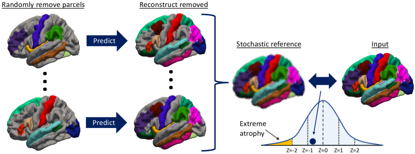
Figure 1: Overview of the stochastic cortex self-reconstruction based on parcels (in color). Parcels are randomly removed and then reconstructed from the remaining ones. This is repeated multiple times to create the stochastic reference cortex, which is then compared to the input for identifying atrophy patterns based on Z-scores. Cortex visualizations with FreeView.

Related Work

Reference and normative models map subject characteristics to brain measurements [21, 29]. Age and sex are commonly used characteristics to predict the reference values [28, 29], which enable the calculation of an individual’s deviation from the norm. Various statistical methods have been introduced for normative modeling, including Gaussian processes [34, 22], Bayesian linear regression [11], hierarchical Bayesian regression [18], quantile regression [20], and generalized additive models of location, scale, and shape (GAMLSS) [4, 6]. The recent creation of brain charts of cortical thickness with GAMLSS aligns closely with our work [4] and will be part of our experiments. The versatility of reference models is demonstrated by their application to a range of brain disorders, including depression, psychosis, schizophrenia, bipolar disorder, autism, and ADHD [27, 21, 3]. Additionally, they were studied in AD [34, 24] and the differential diagnosis of dementia [14], highlighting their considerable potential to enhance the precision in mapping regional brain variations on an individual basis for dementia patients [31]. Normative models are mass-univariate regression models that predict one cortical feature at a time; contrarily, SCSR learns spatial correlations among them across the cortex.

Algorithm 1 Stochastic Cortical Self-Reconstruction

1:Cortical thicknesses for healthy training set $X\in\mathbb{R}^{n,p}$ and test $Y\in\mathbb{R}^{p}$

2:Initialize 2D tensor $T$ of size $p,m$ with NaN values

3:for $i$ = 1 to $m$ do

4:     Randomly partition features of $X$ into predictors $X_{\text{pred}}$ and responses $X_{\text{rep}}$

5:     Train the model $\mathcal{M}_{i}$ to map $X_{\text{pred}}$ to $X_{\text{rep}}$, $\mathcal{M}_{i}:X_{\text{pred}}\mapsto X_{\text{rep}}$

6:     Apply the trained model on test set $\hat{Y}_{\text{rep},i}=\mathcal{M}_{i}(Y_{\text{pred}})$

7:     Store predicted variables $\hat{Y}_{\text{rep},i}$ in the $i$-th slice of tensor $T[:,i]\leftarrow\hat{Y}_{\text{rep},i}$

8:end for

9:Aggregate predictions across iterations $R=\text{percentile}(T,q,\text{axis=2})$ for percentile $q$

10:return $R$, self-reconstruction of healthy cortical thickness reference for $Y$

2 Method

We consider $p$ cortical thickness values for $n$ healthy subjects in the training set $X\in\mathbb{R}^{n,p}$ and a test subject $Y\in\mathbb{R}^{p}$. For the stochastic cortical self-reconstruction, we randomly split the $p$ thicknesses into predictors $X_{\text{pred}}$ and responses $X_{\text{rep}}$, and train a model $\mathcal{M}$ to make the prediction. The model trained on healthy subjects is then applied to healthy or diseased subjects in the test set to predict the missing thicknesses $\hat{Y}_{\text{rep}}=\mathcal{M}(Y_{\text{pred}})$. Repeating this process $m$ times yields $m$ partial reconstructions, which we then aggregate to obtain the final reconstruction of healthy cortical thickness references. Algorithm 1 summarizes the steps in SCSR, and Fig. 1 presents a schematic overview of the idea. In the following, we will introduce three techniques for implementing SCSR.

2.1 XGBoost on Parcels

We use the Desikan-Killiany atlas [5] in FreeSurfer to compute regional cortical thicknesses. Considering one hemisphere at a time, we have $p=34$ parcels in Algorithm 1. We use XGBoost as model $\mathcal{M}$ for the prediction, an efficient implementation of gradient boosting, and among the best-performing methods for tabular data. As XGBoost does not perform multivariate prediction, a separate XGBoost model is trained for each response variable in $X_{\text{rep}}$. For instance, if we select 5 parcels as predictors $X_{\text{pred}}$, 29 XGBoost models would be trained for the 29 responses. This procedure is repeated $m=100$ times to obtain the stochastic self-reconstruction. Further, we evaluate adding age and sex to the predictors. In our experiments, we use a squared error regression objective with a learning rate of 0.15 and a maximum tree depth of 4.

2.2 Autoencoder with MLP

For working on the vertex level, spatial cortex correspondences across subjects need to be established. We follow the procedure in FreeSurfer with inflation, mapping to the sphere, spherical registration to fsvarage6, and resampling [10]. This yields about 40K cortical thickness measures per hemisphere, which will be the input to the network.

The autoencoder performs multivariate prediction so that we simultaneously predict thicknesses for all vertices. It would be impractical to train a separate autoencoder $\mathcal{M}_{i}$ for each random partitioning of the features due to the complexity of training neural networks. Instead, we train a single autoencoder that takes full $X$ as input, but the $X_{\text{rep}}$ part is corrupted. We set the value for those vertices to zero, corresponding to the mean, as we apply the standard scaler to the input data, subtracting the mean per feature. Although the autoencoder returns a full reconstruction, we only keep the reconstruction of the distorted part $\hat{Y}_{\text{rep}}$ to avoid direct propagation through the network. Analogously, the L2 loss between the input and output is only computed on the corrupted part. As architecture, we use three layers with latent dimensions 1,024, batch norm layers with Swift activation in between, and a dropout layer with a rate of 0.5 in the bottleneck. AdamW is used for optimization with a learning rate of 0.001 and weight decay of 0.01.

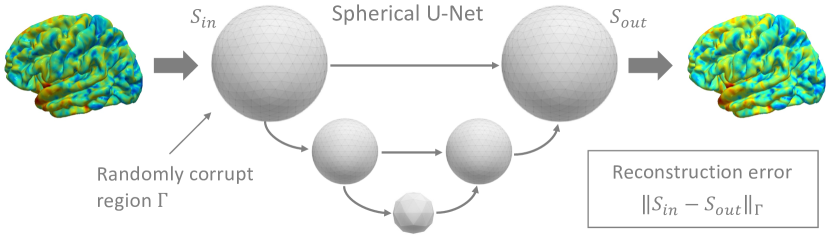
Figure 2: Spherical U-Net operates on spheres with cortical thickness values. Region $\Gamma$ is randomly corrupted on the input sphere $S_{in}$, and the spherical U-Net learns to reconstruct the entire cortical thickness $S_{out}$. The reconstruction loss is only computed on the corrupted region $\Gamma$, or according to prior notation $\|\mathcal{M}(X_{\text{pred}})_{\Gamma}-X_{\text{rep}}\|$.

2.3 Autoencoder with Spherical U-Net

Instead of flattening all vertices as for the MLP, we consider the spherical geometry of the cortex for the reconstruction by designing an autoencoder based on the spherical U-Net [33]. Fig. 2 illustrates the spherical U-Net (S-UNet), which adapts the traditional U-Net architecture to handle spherical data. It is designed for the icosahedron used in FreeSurfer and uses the hierarchical expansion procedure of the icosahedron for up- and downsampling. The convolution layers of the spherical U-Net perform spherical convolutions and, therefore, learn spatial neighborhood relationships on the cortex. We use a spherical U-Net with 5 levels and a channel dimension of 16 at the highest level (doubling at each lower level). We train the network with AdamW, a cyclic learning rate scheduler (decay rate $\gamma=0.9999$), and automatic mixed precision.

2.4 Aggregation and Deviation

For each subject in the test set $Y$, we have $m=100$ partial self-reconstructions stored in the tensor $T$. Across all the predictions, we aggregate the results to obtain a final self-reconstruction for the subject. The mean or median would be natural choices for this. However, pathologic brain changes are related to neuron loss and decreased cortical thickness. If cortex regions affected by atrophy are selected as predictors, this will lead to responses extending the atrophy to the rest of the brain. While many parts of the cortex will be randomly sampled during the stochastic self-reconstruction, we want to emphasize those predictions with higher thickness to create a healthy reference. Hence, we consider not only the median as the 50th percentile but also higher percentiles $q$ in our experiments. We compute the Z-score to quantify the deviation from the norm with $Z=(Y-R)/\sigma$, with the actual thickness of test subject $Y$, SCSR $R$, and standard deviation $\sigma$, estimated from residuals during training.

2.5 Alternative Reference Models

Normative models are the common choice for creating healthy references, using age and sex as input [28, 29]. We compare to a generalized additive model (GAM), specified as $Y\sim\alpha_{0}+f(\text{age})+\alpha_{1}\cdot(\text{sex})$, where $f$ is a smooth spline function estimated based on the data to model the non-linear relationship between thickness and age. Further, we compare to GAMLSS that models next to the mean (location) also the variance (scale), skewness, and kurtosis (shape) of the distribution of the response variable. GAMLSS has previously been used for estimating normative growth curves of CTh, where we specify the first, second, and third order moments similar to ([4], Eq.8) considering coefficients $\alpha,\beta,\gamma$:

$$\mu \sim\alpha_{0}+\alpha_{1}\cdot(\text{age})^{-2}+\alpha_{2}\cdot(\text{age})^{-2}\log(\text{age})+\alpha_{3}\cdot(\text{sex}),$$ (1)

$$\sigma \sim\beta_{0}+\beta_{1}\cdot(\text{age})^{-1}+\beta_{2}\cdot(\text{age})^{0.5}+\beta_{3}\cdot(\text{sex}),$$ (2)

and $\nu\sim\gamma_{0}$. For GAMLSS, we directly predict the standard deviation for the Z-score computation from the model.

3 Results

Data

All models are trained on healthy subjects from the UK Biobank Imaging study [19]. For deployment, we use four datasets with AD patients: the Alzheimer’s Disease Neuroimaging Initiative (ADNI) [16], the Japanese ADNI (J-ADNI) [15], the Australian Imaging, Biomarkers and Lifestyle (AIBL) study [7], and the DZNE-Longitudinal Cognitive Impairment and Dementia Study (DELCODE) [17]. All scans were processed with FreeSurfer to estimate cortical thickness. Automated QC was performed based on the Euler characteristic [9], which represents the number of topological defects and is consistently correlated with visual quality control ratings [26, 23]. Outliers are identified based on the interquartile range method on the Euler characteristics similar to [2, 35, 28]. Table A.1 overviews the public MRI datasets used. In addition, we use routine clinical data from 50 subjects, with an equal distribution of 10 patients per group across AD, posterior cortical atrophy (PCA), behavioral variant frontotemporal dementia (bvFTD), semantic dementia (SD), and normal cognition (CN) for evaluating differential diagnosis. These patients were selected from our hospital database, and diagnosis was established using clinical criteria, FDG-PET metabolism information, and cerebrospinal fluid biomarkers.

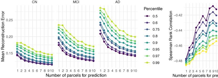
Figure 3: Reconstruction error and Spearman correlation across diagnostic groups for varying the number of parcels and the percentile for the aggregation for XGBoost.

XGBoost

Fig. 3 shows the reconstruction error with XGBoost for the three diagnostic groups averaged across all datasets when varying the number of parcels for the prediction and the aggregation percentile $q$. First, we note an increase in reconstruction error with the progression of dementia, demonstrating that healthy references are created. Second, we note more accurate reconstructions when using more parcels in the prediction, which is to be expected as more information is available for self-reconstruction. Third, moving towards higher percentiles from the median increases the error. The reconstruction errors for GAMLSS are CN: 0.16, MCI: 0.19, AD: 0.23. Due to space, we only show results for the left cortex, with similar results for the right cortex in Fig. 0.A.3.

Fig. 3 also shows the Spearman rank correlation between the AD-ROI Z-score and the ordinal variable diagnosis. The AD-ROI is the average of five regions whose CTh is most affected by AD [30]: entorhinal, inferior temporal, middle temporal, inferior parietal, and fusiform. Here, a strong negative correlation indicates detected atrophy as dementia is progressing. The strongest correlations are obtained with few parcels (1-2) and high percentiles. For comparison, we computed the Spearman correlations of normative models (GAM: -0.44, GAMLSS: -0.46), indicating that many XGBoost configurations yield stronger correlations. Adding age and sex as additional predictors yields slightly lower reconstruction errors for using few parcels (Fig. 0.A.1) but weaker correlations (Fig. 0.A.2). Given our focus is not on the reconstruction error per se but rather on relative differences between groups and a strong correlation, we proceed without considering age and sex as additional predictors.

Autoencoder

Figs. 4 and 5 illustrate the same metrics for the MLP and S-UNet, respectively, with the percentage of uncorrupted vertices along the x-axis. The overall tendency for higher reconstruction errors with more corruption and higher percentiles is analogous to XGBoost. MLP achieves a lower error than the other methods. Further, the strongest correlation of MLP for 15% corruption and high percentiles reaches $-0.55$, clearly stronger than about $-0.48$ for XGBoost and $-0.46$ for GAMLSS. For S-UNet, high corruption rates of 99% yield the strongest correlations, and correlations remain stable below $-0.51$ for all configurations.

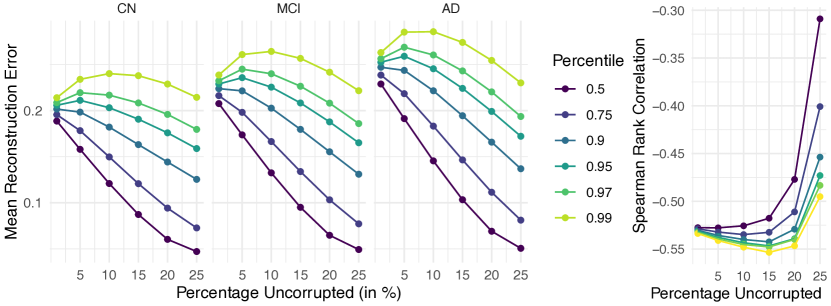
Figure 4: Reconstruction error and Spearman correlation across diagnostic groups for varying the number of parcels and the percentile for the aggregation for MLP.

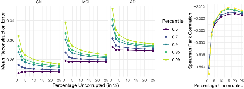
Figure 5: Reconstruction error and Spearman correlation across diagnostic groups for varying the number of parcels and the percentile for the aggregation for S-UNet.

Fig. 6 visualizes vertex-wise average Z-scores for the four dementia groups and CN in the clinical dataset, where we selected S-UNet due to stable correlations in the prior comparison. In all four diagnostic patient groups, we see localized areas with highly negative Z-scores, indicating cortical atrophy in these areas. For bvFTD patients, SCSR indicates lower CTh in prefrontal regions and lateral temporal cortical areas, considered a hallmark finding on MRI in these patients. Fig. 0.A.4 illustrates Z-score maps for all 10 bvFTD patients, demonstrating the ability to highlight individual deviations. As indicated by its name, posterior cortical atrophy is characterized by atrophy in parietal and occipital cortical areas, highlighted with the strongest deviations. We appreciate abnormal CTh in the temporoparietal junction in AD, as well as in the posterior cingulate and mesial temporal lobe. SD leads to a loss of semantic memory and language comprehension, with an expected atrophy in the anterior temporal lobes. In conclusion, SCSR indicates dementia-specific areas of regional atrophy in a clinical patient cohort aligning with established neuroimaging findings [25].

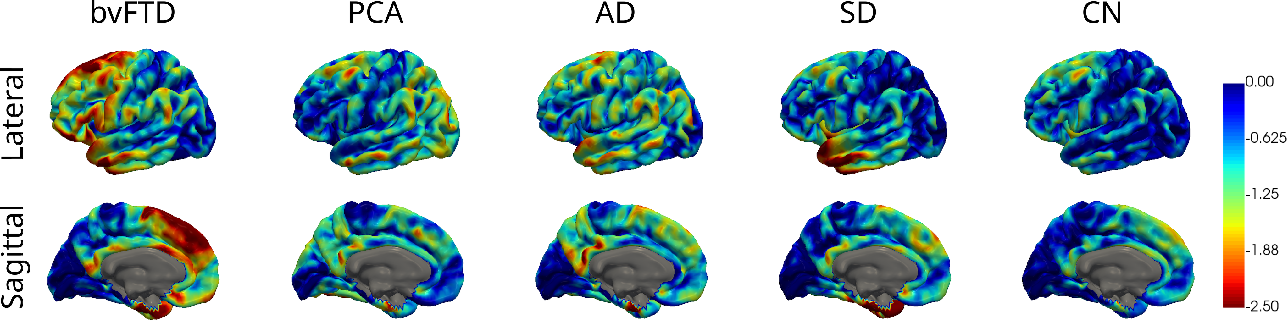
Figure 6: Average Z-scores for the left hemisphere for five diagnostic groups of the clinical dataset. References were estimated with S-UNet (uncorrupted: 1%, $q=.95$).

4 Conclusion

We introduced stochastic cortical self-reconstruction, a new concept for creating a healthy reference to compare cortical thickness. SCSR repeatedly removes part of the cortex and self-reconstructs based on the remaining information. We provided three implementations of this concept, including gradient boosting on parcels and vertex-level autoencoders with MLPs and spherical U-Net. The aggregation of the stochastic reconstructions yields a healthy reference, which is then compared to the true CTh for identifying atrophy patterns. After training on healthy subjects from the UK Biobank, our results on four AD datasets demonstrated the strong correlation of Z-scores with diagnosis. On a clinical dataset with four types of dementia, the high spatial resolution enabled the detailed identification of atrophy patterns needed for differential diagnosis. All results demonstrated the robust generalization to unseen datasets.

5 Acknowledgment

This research was partially supported by the German Research Foundation. The authors gratefully acknowledge the Leibniz Supercomputing Centre by providing computing time on its Linux-Cluster.

Data collection and sharing for this project was funded by the Alzheimer’s Disease Neuroimaging Initiative (ADNI) (National Institutes of Health Grant U01 AG024904) and DOD ADNI (Department of Defense award number W81XWH-12-2-0012). ADNI is funded by the National Institute on Aging, the National Institute of Biomedical Imaging and Bioengineering, and through generous contributions from the following: Alzheimer’s Association; Alzheimer’s Drug Discovery Foundation; Araclon Biotech; BioClinica, Inc.; Biogen Idec Inc.; Bristol-Myers Squibb Company; Eisai Inc.; Elan Pharmaceuticals, Inc.; Eli Lilly and Company; EuroImmun; F. Hoffmann-La Roche Ltd and its affiliated company Genentech, Inc.; Fujirebio; GE Healthcare; ; IXICO Ltd.; Janssen Alzheimer Immunotherapy Research & Development, LLC.; Johnson & Johnson Pharmaceutical Research & Development LLC.; Medpace, Inc.; Merck & Co., Inc.; Meso Scale Diagnostics, LLC.; NeuroRx Research; Neurotrack Technologies; Novartis Pharmaceuticals Corporation; Pfizer Inc.; Piramal Imaging; Servier; Synarc Inc.; and Takeda Pharmaceutical Company. The Canadian Institutes of Health Research is providing funds to support ADNI clinical sites in Canada. Private sector contributions are facilitated by the Foundation for the National Institutes of Health (www.fnih.org). The grantee organization is the Northern California Institute for Research and Education, and the study is coordinated by the Alzheimer’s Disease Cooperative Study at the University of California, San Diego. ADNI data are disseminated by the Laboratory for Neuro Imaging at the University of Southern California.

J-ADNI was supported by the following grants: Translational Research Promotion Project from the New Energy and Industrial Technology Development Organization of Japan; Research on Dementia, Health Labor Sciences Research Grant; Life Science Database Integration Project of Japan Science and Technology Agency; Research Association of Biotechnology (contributed by Astellas Pharma Inc., Bristol-Myers Squibb, Daiichi-Sankyo, Eisai, Eli Lilly and Co., Merck-Banyu, Mitsubishi Tanabe Pharma, Pfizer Inc., Shionogi & Co., Ltd., Sumitomo Dainippon, and Takeda Pharmaceutical Company), Japan, and a grant from an anonymous foundation.

Data used in the preparation of this article were obtained from the Australian Imaging Biomarkers and Lifestyle Flagship Study of Ageing (AIBL) funded by the Commonwealth Scientific and Industrial Research Organisation (CSIRO), which was made available at the ADNI database (www.loni.ucla.edu/ADNI).

Appendix 0.A Supplementary Material

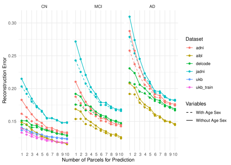
Figure 0.A.1: Reconstruction error for XGBoost and $q=.97$ for (i) different datasets, (ii) integration of age and sex, (iii) varying number of parcels, and (iv) diagnostic group. Particularly for few parcels, the addition of age and sex yields a slightly lower error.

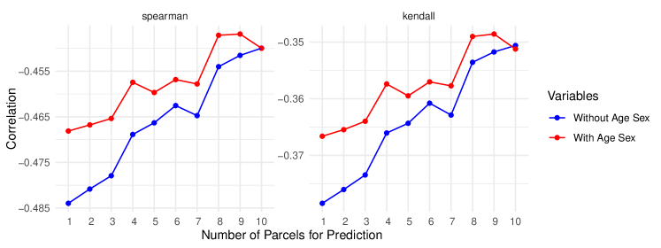
Figure 0.A.2: Spearman rank correlation and Kendall tau for the correlation of Z-scores from XGBoost ($q=.97$) with diagnosis. A stronger negative correlation is obtained for the prediction without age and sex, and with few parcels.

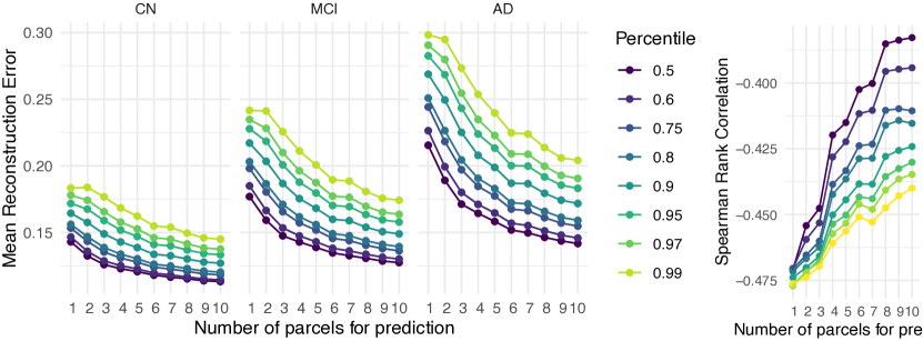
Figure 0.A.3: Reconstruction error and Spearman correlation across diagnostic groups for varying the number of parcels and the percentile for the aggregation for XGBoost on the right hemisphere. The results are similar to the left hemisphere, which we focused on in the rest of the paper, due to limited space. For comparison, GAM and GAMLSS right hemisphere reconstruction error for CN: 0.16, MCI: 0.19, AD: 0.23. Spearman rank correlation for right hemisphere for GAM: -0.42 and GAMLSS: -0.45.

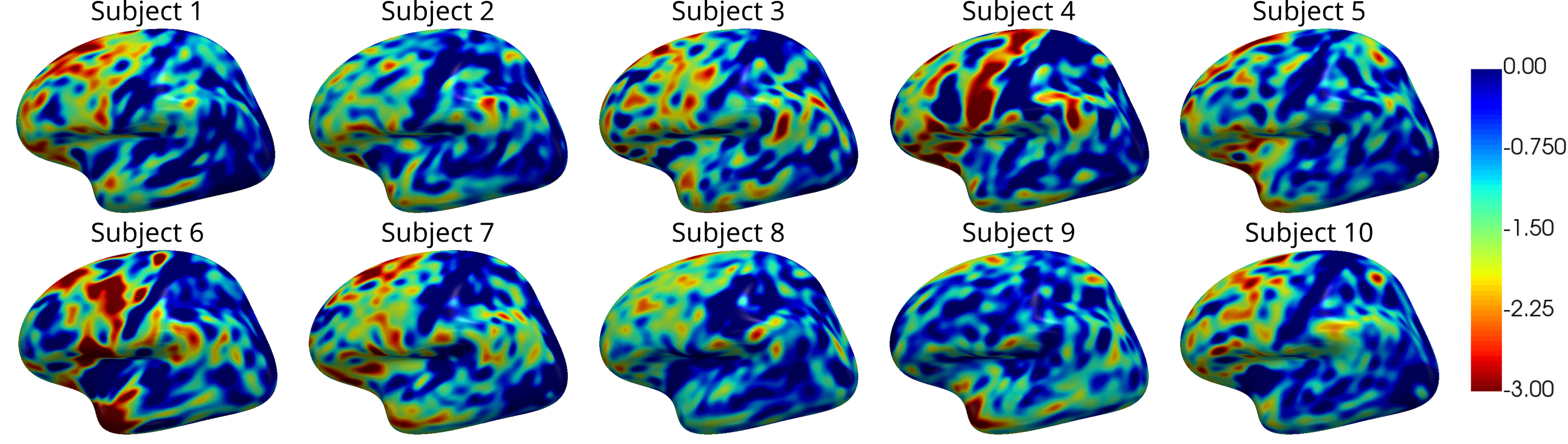
Figure 0.A.4: Single subject Z-scores for all 10 bvFTD patients in the clinical data on the inflated surface. S-UNet with training on UKB was used, demonstrating the generalization across datasets and individual-level utility of SCSR.

Dataset	Subjects	Sex (% M/F)	Age (Mean, SD)	CN	MCI	AD
UK Biobank	31,673	47.3 / 52.7	64.0 (7.5)	31,673	0	0
ADNI	1,521	53.8 / 46.2	73.0 (7.3)	419	822	280
J-ADNI	484	46.5 / 53.5	71.9 (6.4)	141	209	134
AIBL	259	36.7 / 63.3	71.0 (6.1)	196	42	21
DELCODE	447	44.7 / 55.3	71.5 (6.1)	213	141	93

Table A.1: Characteristics of public datasets (MCI: mild cognitive impairment).

References

- [1] Alfaro-Almagro, F., McCarthy, P., Afyouni, S., Andersson, J.L., Bastiani, M., Miller, K.L., Nichols, T.E., Smith, S.M.: Confound modelling in uk biobank brain imaging. NeuroImage 224, 117002 (2021)
- [2] Backhausen, L.L., Herting, M.M., Tamnes, C.K., Vetter, N.C.: Best practices in structural neuroimaging of neurodevelopmental disorders. Neuropsychology Review 32(2), 400–418 (2022)
- [3] Bethlehem, R.A., Seidlitz, J., Romero-Garcia, R., Trakoshis, S., Dumas, G., Lombardo, M.V.: A normative modelling approach reveals age-atypical cortical thickness in a subgroup of males with autism spectrum disorder. Communications biology 3(1), 486 (2020)
- [4] Bethlehem, R.A., Seidlitz, J., White, S.R., Vogel, J.W., Anderson, K.M., Adamson, C., Adler, S., Alexopoulos, G.S., Anagnostou, E., Areces-Gonzalez, A., et al.: Brain charts for the human lifespan. Nature 604(7906), 525–533 (2022)
- [5] Desikan, R.S., Ségonne, F., Fischl, B., Quinn, B.T., Dickerson, B.C., Blacker, D., Buckner, R.L., Dale, A.M., Maguire, R.P., Hyman, B.T., Albert, M.S., Killiany, R.J.: An automated labeling system for subdividing the human cerebral cortex on MRI scans into gyral based regions of interest. NeuroImage (2006)
- [6] Dinga, R., Fraza, C.J., Bayer, J.M., Kia, S.M., Beckmann, C.F., Marquand, A.F.: Normative modeling of neuroimaging data using generalized additive models of location scale and shape. BioRxiv pp. 2021–06 (2021)
- [7] Ellis, K.A., Bush, A.I., Darby, D., et al.: The australian imaging, biomarkers and lifestyle (aibl) study of aging. International psychogeriatrics 21(4), 672–687 (2009)
- [8] Fischl, B.: Freesurfer. Neuroimage 62(2), 774–781 (2012)
- [9] Fischl, B., Liu, A., Dale, A.M.: Automated manifold surgery: constructing geometrically accurate and topologically correct models of the human cerebral cortex. IEEE transactions on medical imaging 20(1), 70–80 (2001)
- [10] Fischl, B., Sereno, M.I., Dale, A.M.: Cortical surface-based analysis: Ii: inflation, flattening, and a surface-based coordinate system. Neuroimage (1999)
- [11] Fraza, C.J., Dinga, R., Beckmann, C.F., Marquand, A.F.: Warped bayesian linear regression for normative modelling of big data. Neuroimage 245, 118715 (2021)
- [12] Frisoni, G.B., Fox, N.C., Jack Jr, C.R., Scheltens, P., Thompson, P.M.: The clinical use of structural mri in alzheimer disease. Nature Reviews Neurology (2010)
- [13] Harper, L., Barkhof, F., Fox, N.C., Schott, J.M.: Using visual rating to diagnose dementia: a critical evaluation of mri atrophy scales. Journal of Neurology, Neurosurgery & Psychiatry 86(11), 1225–1233 (2015)
- [14] Hedderich, D.M., Dieckmeyer, M., Andrisan, T., Ortner, M., Grundl, L., Schön, S., Suppa, P., Finck, T., Kreiser, K., Zimmer, C., et al.: Normative brain volume reports may improve differential diagnosis of dementing neurodegenerative diseases in clinical practice. European Radiology 30, 2821–2829 (2020)
- [15] Iwatsubo, T.: Japanese alzheimer’s disease neuroimaging initiative: present status and future. Alzheimer’s & Dementia 6(3), 297–299 (2010)
- [16] Jack Jr, C.R., Bernstein, M.A., Fox, N.C., Thompson, P., et al.: The alzheimer’s disease neuroimaging initiative (adni): Mri methods. Journal of Magnetic Resonance Imaging 27(4), 685–691 (2008)
- [17] Jessen, F., Spottke, A., Boecker, H., et al.: Design and first baseline data of the dzne multicenter observational study on predementia alzheimer’s disease (delcode). Alzheimer’s research & therapy 10(1), 1–10 (2018)
- [18] Kia, S.M., Huijsdens, H., Dinga, R., Wolfers, T., Mennes, M., Andreassen, O.A., Westlye, L.T., Beckmann, C.F., Marquand, A.F.: Hierarchical bayesian regression for multi-site normative modeling of neuroimaging data. In: MICCAI (2020)
- [19] Littlejohns, T.J., Holliday, J., Gibson, L.M., et al.: The uk biobank imaging enhancement of 100,000 participants: rationale, data collection, management and future directions. Nature communications 11(1), 2624 (2020)
- [20] Lv, J., Di Biase, M., Cash, R.F., et al.: Individual deviations from normative models of brain structure in a large cross-sectional schizophrenia cohort. Molecular psychiatry 26(7), 3512–3523 (2021)
- [21] Marquand, A.F., Kia, S.M., Zabihi, M., Wolfers, T., Buitelaar, J.K., Beckmann, C.F.: Conceptualizing mental disorders as deviations from normative functioning. Molecular psychiatry 24(10), 1415–1424 (2019)
- [22] Marquand, A.F., Rezek, I., Buitelaar, J., Beckmann, C.F.: Understanding heterogeneity in clinical cohorts using normative models: beyond case-control studies. Biological psychiatry 80(7), 552–561 (2016)
- [23] Monereo-Sanchez, J., de Jong, J.J., Drenthen, G.S., Beran, M., Backes, W.H., Stehouwer, C.D., Schram, M.T., Linden, D.E., Jansen, J.F.: Quality control strategies for brain mri segmentation and parcellation. Neuroimage 237, 118174 (2021)
- [24] Potvin, O., Dieumegarde, L., Duchesne, S., Initiative, A.D.N., et al.: Normative morphometric data for cerebral cortical areas over the lifetime of the adult human brain. Neuroimage 156, 315–339 (2017)
- [25] Risacher, S.L., Saykin, A.J.: Neuroimaging biomarkers of neurodegenerative diseases and dementia. In: Seminars in neurology. pp. 386–416 (2013)
- [26] Rosen, A.F., Roalf, D.R., Ruparel, K., Blake, J., Seelaus, K., Villa, L.P., Ciric, R., Cook, P.A., Davatzikos, C., Elliott, M.A., et al.: Quantitative assessment of structural image quality. Neuroimage 169, 407–418 (2018)
- [27] Rutherford, S., Barkema, P., Tso, I.F., Sripada, C., Beckmann, C.F., Ruhe, H.G., Marquand, A.F.: Evidence for embracing normative modeling. Elife 12 (2023)
- [28] Rutherford, S., Fraza, C., Dinga, R., Kia, S.M., Wolfers, T., Zabihi, M., Berthet, P., Worker, A., Verdi, S., Andrews, D., et al.: Charting brain growth and aging at high spatial precision. elife 11, e72904 (2022)
- [29] Rutherford, S., Kia, S.M., Wolfers, T., Fraza, C., Zabihi, M., Dinga, R., Berthet, P., Worker, A., Verdi, S., Ruhe, H.G., et al.: The normative modeling framework for computational psychiatry. Nature protocols 17(7), 1711–1734 (2022)
- [30] Schwarz, C.G., Gunter, J.L., Wiste, H.J., et al.: A large-scale comparison of cortical thickness and volume methods for measuring alzheimer’s disease severity. NeuroImage: Clinical 11, 802–812 (2016)
- [31] Verdi, S., Marquand, A.F., Schott, J.M., Cole, J.H.: Beyond the average patient: how neuroimaging models can address heterogeneity in dementia. Brain (2021)
- [32] Wahlund, L.O., Westman, E., van Westen, D., Wallin, A., Shams, S., Cavallin, L., Larsson, E.M.: Imaging biomarkers of dementia: recommended visual rating scales with teaching cases. Insights into imaging 8, 79–90 (2017)
- [33] Zhao, F., Xia, S., Wu, Z., Duan, D., Wang, L., Lin, W., Gilmore, J.H., Shen, D., Li, G.: Spherical u-net on cortical surfaces: Methods and applications. In: Information Processing in Medical Imaging. p. 855–866 (2019)
- [34] Ziegler, G., Ridgway, G.R., Dahnke, R., Gaser, C., Initiative, A.D.N., et al.: Individualized gaussian process-based prediction and detection of local and global gray matter abnormalities in elderly subjects. NeuroImage 97, 333–348 (2014)
- [35] Zugman, A., Harrewijn, A., Cardinale, E.M., Zwiebel, H., Freitag, G.F., Werwath, K.E., Bas-Hoogendam, J.M., Groenewold, N.A., Aghajani, M., Hilbert, K., et al.: Mega-analysis methods in enigma. Human Brain Mapping (2022)