NeuPAN: Direct Point Robot Navigation with End-to-End Model-based Learning

Abstract

Navigating a nonholonomic robot in a cluttered environment requires extremely accurate perception and locomotion for collision avoidance. This paper presents NeuPAN: a real-time, highly-accurate, map-free, robot-agnostic, and environment-invariant robot navigation solution. Leveraging a tightly-coupled perception-locomotion framework, NeuPAN has two key innovations compared to existing approaches: 1) it directly maps raw points to a learned multi-frame distance space, avoiding error propagation from perception to control; 2) it is interpretable from an end-to-end model-based learning perspective, enabling provable convergence. The crux of NeuPAN is to solve a high-dimensional end-to-end mathematical model with various point-level constraints using the plug-and-play (PnP) proximal alternating-minimization network (PAN) with neurons in the loop. This allows NeuPAN to generate real-time, end-to-end, physically-interpretable motions directly from point clouds, which seamlessly integrates data- and knowledge-engines, where its network parameters are adjusted via back propagation. We evaluate NeuPAN on car-like robot, wheel-legged robot, and passenger autonomous vehicle, in both simulated and real-world environments. Experiments demonstrate that NeuPAN outperforms various benchmarks, in terms of accuracy, efficiency, robustness, and generalization capability across various environments, including the cluttered sandbox, office, corridor, and parking lot. We show that NeuPAN works well in unstructured environments with arbitrary-shape undetectable objects, making impassable ways passable.

I Introduction

Navigating a robot in a densely confined environment in real-time is crucial for a broad range of applications from machine housekeeper (e.g., mobile ALOHA [1]) to autonomous parking (e.g., Tesla FSD [2]). In contrast to wide-open environments, the aforementioned cluttered scenarios require robot perceptions (i.e., providing necessary information about the environment) and motions (i.e., computing a sequence of feasible actions to connect the current and target states) to be very accurate under dynamic (e.g., Ackermann steering) and kinematic (e.g., collision avoidance) constraints; otherwise, efficiency or safety could be greatly compromised. The situation becomes even more nontrivial if the navigation system needs to work properly in new environments on new robots.

Existing approaches fail to address the problem due to the following: 1) Compressing a high-dimensional sensor space (e.g., millions of points per second) into a low-dimensional action space (e.g., throttle and steer) with no error propagation while guaranteeing interpretability is nontrivial [3, 4]; 2) The navigation problem is $\mathsf{PSPACE}$ hard, and existing solutions [5, 6, 7] have to balance the trade-off between accuracy and complexity, resulting in either inexact motions (prone to get stuck) or delayed motions (prone to collisions); 3) The solution should be stable, complete, and easy-to-use, involving little hand-engineering and training for new robots and environments [8, 9]. The above system, algorithm, and engineering issues make dense-scenario navigation with only the onboard computation resources a long-standing challenge.

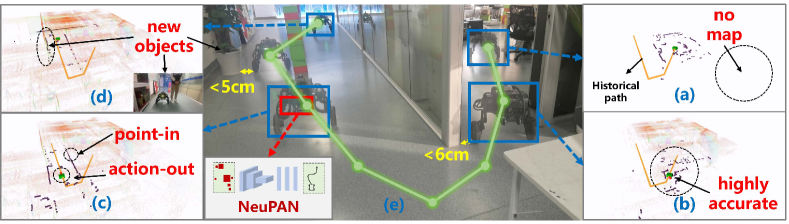
Figure 1: (a) NeuPAN navigates a wheel-legged robot with no prior map. (b) robot navigates through narrow gaps($<6\,$cm); (c) NeuPAN operates in a “point-in action-out” manner at a frequency of $20\,$Hz; (d) NeuPAN generalizes to handling out-of-distribution (moving) objects. (e) Trajectory of the wheel-legged robot empowered by NeuPAN.

To address all these issues, this paper proposes a LiDAR-based end-to-end model-based learning approach, termed NeuPAN, to achieve real-time (e.g., $20\,$Hz), highly accurate (e.g., $3\,$cm), map-free (e.g., suitable for exploration), robot-agnostic (i.e., direct deployment on new robots), and environment-invariant (i.e., no retraining across different scenarios) collision avoidance. Our solution chooses the LiDAR sensor due to its ability to provide direct, dense, active, and accurate depth measurements of environments, as well as its insensitivity to illumination variation and motion blur (as opposed to vision-based solutions). The considerably reduced cost, size, weight, and power of emerging LiDARs (e.g., solid-state LiDAR) make our solution promising for a broad scope of robotic applications. Building upon these inherent features of LiDAR hardware, and empowered by the software packages of our NeuPAN, a wheel-legged robot is able to navigate through narrow gaps with arbitrary shapes without a prior map while avoiding collisions with unknown dyanmic objects outside the training dataset, as demonstrated in Fig. 1.

The key contributions that lead to the superior performance of our system are as follows: 1) In contrast to existing approaches that convert point clouds to convex sets or occupancy grids, and adopt inexact collision distances, NeuPAN directly processes high-dimensional raw points and computes the point flow based on ego-motion. Then a neural encoder is leveraged to map point flow to a multi-frame distance feature, which corresponds to the exact distance from the ego-robot to any object at any time step within the receding horizon. 2) The learnt distance features are seamlessly incorporated into the motion planner as a norm regularizer added to the loss function, accounting for the reward of departure from obstacles. The future states and actions generated by the motion planner are fed back to the front-end for re-computation of the point flow. This forms a tightly-coupled loop between perception and locomotion. 3) To gain deeper insights into NeuPAN, we formulate an end-to-end mathematical program with the number of constraints equal to the number of laser scans. It is found that NeuPAN is equivalent to solving this naturalistic problem using the plug-and-play (PnP) proximal alternating-minimization (PAN) algorithm. For the first time, a navigation algorithm is interpreted from a model-based learning perspective, thus seamlessly integrating data-driven systems with rigorous mathematical models. 4) We conduct various experiments to evaluate the effectiveness of the developed neural encoder, the motion planner, and the overall NeuPAN system. Experiments on the KITTI and SUSCAPE datasets show that the neural encoder achieves a distance error significantly smaller than the best detector. Exhaustive benchmark comparisons in various simulated indoor and outdoor scenarios show that NeuPAN achieves consistently higher success rates with shorter navigation time at a lower computation load than other state-of-the-art robot navigation systems. We finally show the effectiveness of NeuPAN in real-world dynamic, cluttered, and unstructured environments including the sandbox, office, corridor, and parking lot on agile mobile robots, wheel-legged robots, and passenger autonomous vehicles.

The remainder of this paper is organized as follows. Section II reviews related work. Section III presents the system framework. Subsequently, Section IV and Section V present the neural encoder network and the neural regularized motion planner, respectively. Section VI analyzes the theoretical properties and guarantees. Sections VII and VIII introduce simulation and real-world experiments. Finally, Section IX concludes this work.

II Related Work

II-A Modular vs. End-to-End

Modular approaches, which divide navigation into distinct modules (e.g., an object detector and a motion planner in the simplest case), are the most widely adopted framework due to its reliability and ease of debugging [10, 11, 12]. However, these approaches suffer from error propagation from perception to control modules: 1) At the front-end perception layer, the bounding box generated by even the best detector can deviate from the ground truth by a meter-level distance, making it inevitable to incorporate a meter-level safety distance in the motion planner to guarantee worst-case collision avoidance; 2) At the intermediate representation layer, the box (or convex sets by using more advanced detectors) cannot exactly match the real-world objects that may possess arbitrary nonconvex shapes; 3) At the back-end planning layer, approximations may be introduced to compute the distance between any two bodies. The above three distance errors in individual layers will add up together to the navigation pipeline, making modular approach prone to get stuck in cluttered environments.

To mitigate the error propagation inherent in the modular approach, recent robot navigation is experiencing a paradigm shift towards an end-to-end approach, which directly maps sensor inputs to motion outputs [13, 9, 14]. Earlier end-to-end solutions focused on using a single black-box deep neural network (DNN) to learn the mapping but were later found difficult to train and not generalizable to unseen situations. The emerging end-to-end approach adopts multiple blocks but differs from the modular approach in three aspects: 1) it exchanges features (e.g., encoder outputs) instead of explicit representations (e.g., bounding boxes) among modules; 2) the interaction among modules is bidirectional instead of unidirectional; 3) the entire system can be trained in an end-to-end manner. Such generalized end-to-end approaches have shown effectiveness in vision-based autonomous driving and encoder-based robot manipulation. For instance, the Unified Autonomous Driving (UniAD) framework consists of backbone, perception, prediction, and planning modules, with task queries as interfaces connecting each node [15]. In practice, companies such as Tesla, Horizon Robotics, XPeng, also exploited end-to-end approaches, which leverage vision transformers to generate bird’s eye view (BEV)  [16] for occupancy mapping [17] that is directly used for subsequent planning. Similar insights have been obtained for robot manipulation, which can be accomplished by a Motion Planning Network (MPNet) consisting of a neural encoder and a motion planner [18]. The limitation of these purely data-driven techniques lies in their lack of interpretability. This makes it difficult to adjust the network parameters for new robot platforms. When generalizing to a new environment, they often require extensive hand-engineering and prolonged training and usually need to be accompanied by other conservative strategies to guarantee safety. These methods also demand significant data collection and annotation efforts.

Our framework belongs to the generalized end-to-end approach since 1) it directly maps raw points to distance features rather than sets; 2) the perception and locomotion are tightly-coupled through closed-loop iteration; 3) the system can be trained in an end-to-end fashion. However, our method differs from existing end-to-end solutions such as UniAD and MPNet by providing additional mathematical interpretability and guarantee. This enables our system to generate very accurate and safe robot motions without uncertainties, as we show in the experiments in Sections VII and VIII.

II-B Model-based vs. Learning-based

Algorithms determine the inference mapping of each module in modular or end-to-end frameworks. Existing algorithms can be categorized into model-based and learning-based.

Model-based algorithms utilize mathematical or statistical formulations that represent the underlying physics, prior information, and domain knowledge. Very often, this type of algorithm is used within the modular framework for solving the back-end motion planning problem. Classical model-based algorithms include graph search-based, sampling-based, and optimization-based. Graph search-based techniques, e.g., A^∗, approximate the configuration space as a discrete grid space to search the path with minimum cost [19]. Sampling-based techniques, e.g., rapidly-exploring random tree (RRT) or RRT^∗, probe the configuration space with a sampling strategy [20]. Optimization based techniques generate trajectories through minimizing cost functions under dynamics and kinematics constraints [3, 11].

In the context of dense-scenario navigation, optimization-based techniques, such as model predictive control (MPC), are more attractive due to their ability to compute the current optimal input to produce the best possible behavior in the future, resulting in high-performance trajectories. The main drawback of optimization-based techniques is their high computational cost, which limits their real-time applications. This is because the number of collision avoidance constraints is proportional to the number of obstacles (spatial) and the length of the receding horizon (temporal). In cluttered environments, where the shape of obstacles is also taken into account, the computation time is further multiplied by the number of surfaces from each obstacle. To reduce the complexity, the optimization-based collision avoidance (OBCA) algorithm is developed in [3] for full-shape MPC, which adopts duality to handle the exact distance between the obstacle and the ego-robot. Moreover, full-shape robot navigation is further accelerated by a space-time decomposition algorithm in [21]. However, the frequency of these algorithms is not satisfactory, e.g., approximately $1\,$ Hz when dealing with tens of objects. On the other hand, most existing works forgo exact distances and adopt inexact ones, such as center-point distances, approximate signed distances, or spatial-temporal corridors [22, 23]. Additionally, it is possible to convert hard constraints into soft regularizers for speed-up, as exemplified by the EGO planner, which removes the collision avoidance constraints by adding penalty terms [24]. While inexact algorithms achieve a high frequency (e.g., up to $100\,$Hz), they are not suitable for dense-scenario navigation, as discussed earlier in Section I.

TABLE I: Comparison with state-of-the-art approaches

Scheme	System Input	Full Shape	Exact distance	Map Free	Generalization	Latency†	Constraints Guarantee
TEB [5]	Grids	✔	✗	✗	✔	Low	✔
OBCA [3]	Object Sets	✔	✔	✗	✔	High	✔
RDA [21]	Object Sets	✔	✔	✔	✔	Medium$\sim$high	✔
STT [23]	Object Sets	✔	✗	✗	✔	Low	✗
AEMCARL [25]	Object Poses	✗	N/A	✔	✗	Low	✗
Hybrid-RL [9]	Lidar Points	✗	N/A	✔	✗	Low	✗
MPC-MPNet [18, 26]	Lidar Points	✔	✗	✔	✗	Low	✔
NeuPAN (Ours)	Lidar Points	✔	✔	✔	✔	Low$\sim$Medium	✔

${\dagger}$ low latency: $<50\,$ms; medium latency: $50\sim 500\,$ms; high latency: $>500\,$ms.

In contrast to model-based approaches, learning algorithms dispense with analytical models by extracting features from data. This is particularly useful in complex systems where analytical models are not known. Consequently, learning algorithms are promising for perception and end-to-end navigation tasks. In this direction, reinforcement learning (RL) and imitation learning (IL) are two major paradigms [27]. The idea of RL is to learn a neural network policy by interacting with the environment and maximizing cumulative action rewards [28]. In particular, RL has been widely used for the dynamic collision avoidance, termed CARL based approaches, where the motion information of obstacles is mapped to the robot actions directly, such as CADRL [29], LSTM-RL [30], SARL [8], RGL [31], and AEMCARL [25], etc.. However, the performance of RL-based methods is influenced by the training dataset’s distribution. Therefore, these methods are promising in simulation but often challenging to implement in real-world settings. Additionally, finding a suitable reward function for dense-scenario navigation is often difficult. On the other hand, IL generates neural policies by learning from human demonstrations, thereby narrowing the gap between simulation and reality. In particular, IL methods have been validated in self-driving cars [32], where a convolutional neural network is developed to map images to actions. Building upon [32], conditional IL is utilized for more complex situations that require decision-making [33]. The development of IL is hindered by the requirement for a large volume of training data, including both sensor inputs and expert control outputs.

As mentioned in Section II-A, learning-based algorithms lack interpretability. Hence, an emerging paradigm involves the cross-fertilization of model-based and learning-based algorithms. This has led to a variety of model-based learning approaches in robot navigation. In particular, a direct way is to use learning algorithms to imitate complex dynamics or numerical procedures by transforming iterative computations into a feed-forward procedure. This is achieved by learning from solvers’ demonstrations using DNNs. Examples include the neural PID in [34] and the neural MPC in [35]. On the other hand, learning-based algorithms are adopted to generate candidate trajectories, reducing the solution space for subsequent model-based algorithms, e.g., MPNet [18], MPC-MPNet [26], NFMPC [36], and MPPI [37]. Note that trajectory generation is often learned from classical sampling-based approaches. Lastly, learning algorithms can be used to adjust the hyper-parameters involved in model-based algorithms. For instance, the cost and dynamics terms of MPC can be learned by differentiating parameters with respect to the policy function through the optimization problem [38, 39].

Our framework, NeuPAN, also belongs to the model-based deep learning approach. However, in contrast to the aforementioned works that are partially interpretable, NeuPAN is end-to-end interpretable from perception, to planning, and to control. This is achieved by solving a high-dimensional end-to-end optimization problem with numerous point-level constraints using the PnP PAN. This makes NeuPAN suitable for dense-scenario collision avoidance with nonholonomic robots, whereas existing results [24, 9, 23] usually consider holonomic drones or nonholonomic robots in wide-open scenarios. Similar to [38, 39], parameters within the costs and constraints of NeuPAN can be trained via policy function differentiation in an end-to-end fashion. Hence, NeuPAN finally enjoys robot-agnostic and environment-invariant features.

II-C Limitations of Existing Solutions

Comprehensive comparison with state-of-the-art navigation approaches is provided in Table I. In particular, TEB [5], OBCA [3], RDA [21], STT [23], and AEMCARL [25] are modular approaches. Their inputs are grids, poses, boxes, or sets generated by a pre-established grid map or a front-end object detector. All these methods involve error propagation. In contrast to AEMCARL which treats the ego-robot as a point (or ball), TEB, OBCA, RDA, and STT consider the shape of the ego-robot and obstacles. However, TEB and STT involve approximations when computing the distance between two shapes. OBCA and RDA are the most accurate approaches but require high computational latency, e.g., up to second-level (i.e., less than $1\,$Hz). On the other hand, Hybrid-RL [9], MPC-MPNet [26], and NeuPAN (ours) are end-to-end approaches. By treating raw LiDAR points as inputs, these methods are free from error propagation. Hybrid-RL adopts a single network for point input and action output. Despite its high-level integration, Hybrid-RL suffers from poor generalization capability. MPC-MPNet, and NeuPAN adopt two networks, one for encoding and the other for planning: MPC-MPNet uses a neural encoder to map points into voxel features; NeuPAN uses a neural encoder to map points and ego-motions into spatial-temporal distance features. All of them consider the shape of objects; however, due to the discretization from points to voxels, MPC-MPNet cannot compute the exact distances between two shapes. They also lack generalization as the trajectory generator is scenario-dependent and needs retraining for new robots. Our NeuPAN overcomes these drawbacks, at the cost of a slightly higher computational load.

II-D New Features Offered by NeuPAN

NeuPAN is the first approach that builds the end-to-end mathematical model (i.e., point-in and action-out), and uses model-based learning to solve it. As such, NeuPAN is able to push math to its upper limit, until the remaining challenge outside the boundary of math is tackled by neural networks in an interpretable fashion. Owing to this new feature, NeuPAN generates very accurate, end-to-end, physically-interpretable motions in real time. This empowers autonomous systems to work in dense unstructured environments, which are previously considered impassable and not suitable for autonomous operations, triggering new applications such as cluttered-room housekeeper and limited-space parking. Compared to existing end-to-end methods, [13, 9, 14, 15, 16, 17, 18], NeuPAN provides mathematical guarantee and leads to much lower uncertainty and higher generalization capability. Compared to existing model-based motion planning methods [3, 18, 21, 23], NeuPAN is more accurate, since conventional motion planning belongs to modular approaches and involves error propagation. There also exist other model-based learning methods [34, 35, 18, 36, 37] for robot navigation. However, these methods are not end-to-end, e.g., [34, 35] consider state-in action-out, and [18, 36, 37] consider point-in trajectory-out (similar to Tesla). The work [26] considers point-in action-out, by bridging [18] with a back-end controller. However, such a bridge loses mathematical guarantee and no longer solve the inherent end-to-end model. The methods [26, 18] also leverage neural encoder like transformer to compress the sensor data, and this neural encoder has no interpretability.

III NeuPAN System Overview

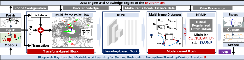
Figure 2: System architecture of NeuPAN, an end-to-end model-based deep learning approach.

III-A Problem Statement

We consider a LiDAR-based robot navigation system with points in and actions out. The input LiDAR raw points are sequentially accumulated into scans that can be viewed as discrete measurements in the time domain. The period between consecutive scans typically ranges from $10\,$ms (for $100\,$Hz update) to $100\,$ms (for $10\,$Hz update). Each LiDAR scan is considered as a time frame. At the $t$-th time frame, the scan $\mathbb{P}_{t}$ is a set of points $\mathbb{P}_{t}=\{\mathbf{p}_{t}^{1},\ldots,\mathbf{p}_{t}^{m},\ldots,\mathbf{p}_{t}^{M}\}$, where $\mathbf{p}_{t}^{m}\in\mathbb{R}^{n}$ is the $n$-dimensional position of the $m$-th LiDAR point in the global coordinate system and $M$ is the total number of points of the $t$-th scan. Given the input scan $\mathbb{P}_{t}$, the system needs to plan a trajectory $\mathcal{S}=\{\mathbf{s}_{t},\cdots,\mathbf{s}_{t+H-1}\}$, where $\mathbf{s}_{t}$ is the robot pose at time $t$ and $H$ is the length of receding horizon. The associated actions are given by $\mathcal{U}=\{\mathbf{u}_{t},\cdots,\mathbf{u}_{t+H-1}\}$, where $\mathbf{u}_{t}$ is the control vector at time $t$. Due to non-holonomic robot dynamics, $\mathcal{S}$ and $\mathcal{U}$ should together satisfy $\{\mathcal{S},\mathcal{U}\}\in\mathcal{F}$, where $\mathcal{F}$ is the feasible set for producing physically reasonable trajectories. The system outputs action $\mathbf{u}_{t}$ to actuate the robot.

The end-to-end perception-planning-control optimization problem is thus

$$\mathsf{P}:\min_{\begin{subarray}{c}\mathcal{S},\mathcal{U}\end{subarray}}~{}~{} C_{0}(\mathcal{S},\mathcal{U})$$ (1a)

s.t. $${\bf{dist}}(\mathbb{Z}_{t+h}(\mathbf{s}_{t+h}),\mathbb{P}_{t+h})\geq d_{\min},~{}\forall h,$$ (1b)

$$\{\mathcal{S},\mathcal{U}\}\in\mathcal{F}.$$ (1c)

Symbol notations for $\mathsf{P}$ are as follows:

• Cost function $C_{0}(\mathcal{S},\mathcal{U})$ is the distance between reference and actual trajectories:

  $$C_{0}(\mathcal{S},\mathcal{U}) =\sum_{h=0}^{H-1}\Big{(}\left\|\mathbf{q}\circ({{\mathbf{s}_{t+h}}-{\mathbf{s}_{t+h}^{\diamond}}})\right\|_{2}^{2}$$

  $$\quad\quad+\left\|\mathbf{p}\circ(\mathbf{u}_{t+h}-{\mathbf{u}_{t+h}^{\diamond}})\right\|_{2}^{2}\Big{)},$$ (2)

  where $\{\mathbf{q},\mathbf{p},\mathbf{s}_{t}^{\diamond},\mathbf{u}_{t}^{\diamond}\}$ are determined by prior knowledge (e.g., historical path) or high-level decision making (e.g., large model).

• Distance function ${\bf{dist}}(\mathbb{Z}_{t}(\mathbf{s}_{t}),\mathbb{P}_{t})$ denotes the minimum Euclidean distance between the ego robot and the $t$-th scan, where $\mathbb{Z}_{t}$ is the set of all points occupied by the robot and is a function of robot pose $\mathbf{s}_{t}$.

Technical Challenge: In general, $\mathbb{P}_{t}$ contains thousands to millions of points, i.e., $M\in[10^{3},10^{6}]$, meaning that computing ${\bf{dist}}(\mathbb{Z}_{t}(\mathbf{s}_{t}),\mathbb{P}_{t})$ itself is a high-dimensional minimization problem. This is why traditional approaches convert $\mathbb{P}_{t}$ to boxes, sets, voxels, or grids for dimension reduction. However, in this paper, we focus on unstructured environments. To keep the most accurate, complete, and dense information about the environments, we propose to directly process $\mathbb{P}_{t}$, resulting in an end-to-end perception-planning-control approach.

III-B NeuPAN System

The system architecture of NeuPAN is shown in Fig. 2, which is an iterative procedure for solving $\mathsf{P}$. In each iteration, NeuPAN transforms raw points (i.e., inputs) to point flow $\mathbb{PF}$ by the transform-based block, then to multi-frame distance (MFD) features by the learning-based block, and finally to robot actions by the model-based block. The solution (i.e., containing both robot actions and the associated trajectories) generated by the model-based block is fed back to the transform-based block for re-generation of point flow, which forms a tightly-coupled closed-loop between perception and locomotion. Below we present the structure of each block.

• Transform-based block. This block generates the multi-frame point flow $\mathbb{PF}$ by aggregating points in a new scan and candidate ego-motions obtained from the last-round iteration. This is realized by transforming each ego-motion into a rotation matrix $\Delta\mathbf{R}$ and a translation vector $\Delta\mathbf{t}$. By taking the inverse of $\Delta\mathbf{R}$ and $\Delta\mathbf{t}$, the state evolution for each point is $\widetilde{\mathbf{p}}_{t+1}^{i}=\Delta\mathbf{R}^{-1}\widetilde{\mathbf{p}}_{t}^{i}-\Delta\mathbf{t}$ for $t=0,\cdots,H-1$, where $\widetilde{\mathbf{p}}_{t}^{i}$ is the point of $\mathbf{p}_{t}^{i}$ in ego-robot local coordinate system. All points $\{\widetilde{\mathbf{p}}_{t}^{i},\widetilde{\mathbf{p}}_{t+1}^{i},\cdots\}$ are collectively denoted as $\mathbb{PF}$.

• Learning-based block. This block leverages a neural encoder to map the point flow to a latent feature space of MFD parameterized by $\mathcal{M}=\{\bm{\mu}_{t}^{i}\}$ and $\mathcal{L}=\{\bm{\lambda}_{t}^{i}\}$, with $\{\mathcal{M},\mathcal{L}\}\in\mathcal{G}$ ($\mathcal{G}$ denotes the domain of latent space). This latent space is used to compute the exact distance from ego-robot to arbitrary LiDAR point at any time slot within the receding horizon (as detailed in Section IV). The encoder is denoted as deep unfolded neural encoder (DUNE), since it can be interpreted as unfolding penalty inexact block coordinate descent (PIBCD) into the DNN.

• Model-based block. The model-based block seamlessly incorporate the learnt MFD features into a motion planning optimization problem as a rigorously-derived regularizer, $C_{r}(\mathcal{S},\mathcal{M},\mathcal{L})$, imposed on the loss function $C_{0}$, accounting for the reward of collision avoidance (as detailed in Section V). With this regularizer, we can safely remove the numerous point-level collision avoidance constraints without any approximation error, which is in contrast to conventional approximation or regularization methods [24, 22, 23] that may lead to constraints over-satisfaction or violation. The resultant problem is neural regularized, hence its associated solver is called neural regularized motion planner (NRMP).

III-C Theoretical Interpretation

The entire procedure can be viewed as iterations between learning-based (i.e., DUNE) and modeled-based (i.e., NRMP) algorithms. Mathematically, this is equivalent to solving

$$\mathsf{Q}:\min_{\begin{subarray}{c}\{\mathcal{S},\mathcal{U}\}\in\mathcal{F},\{\mathcal{M},\mathcal{L}\}\in\mathcal{G}\end{subarray}}~{}~{} \underbrace{C_{0}(\mathcal{S},\mathcal{U})+C_{r}(\mathcal{S},\mathcal{M},\mathcal{L})}_{:=C_{\mathrm{e2e}}(\mathcal{S},\mathcal{U},\mathcal{M},\mathcal{L})}$$ (3)

using PAN framework, where the subproblem of $\{\mathcal{S},\mathcal{U}\}$ is solved using model-based approach while the subproblem of $\{\mathcal{M},\mathcal{L}\}$ is solved using learning-based approach. As shown in Appendix A (detailed in the supporting document), the optimal solution to $\mathsf{Q}$ is also optimal to $\mathsf{P}$. Specifically, given $\{\mathcal{S}^{[k]},\mathcal{U}^{[k]}\}$ of state-action space at the $k$-th iteration, NeuPAN generates the next-round solution $\{\mathcal{S}^{[k+1]},\mathcal{U}^{[k+1]}\}$ as follows:

$$\{\mathcal{S}^{[k]},\mathcal{U}^{[k]}\}\stackrel{{\scriptstyle\mathsf{DUNE}}}{{\longrightarrow}}\{\mathcal{M}^{[k+1]},\mathcal{L}^{[k+1]}\}\stackrel{{\scriptstyle\mathsf{NRMP}}}{{\longrightarrow}}\{\mathcal{S}^{[k+1]},\mathcal{U}^{[k+1]}\}.$$

Consequently, starting from an initial guess $\{\mathcal{S}^{[0]},\mathcal{U}^{[0]}\}$, the sequence generated by NeuPAN is

$$\{\mathcal{S}^{[0]},\mathcal{U}^{[0]}\} \stackrel{{\scriptstyle\mathsf{DUNE}}}{{\longrightarrow}}\{\mathcal{M}^{[1]},\mathcal{L}^{[1]}\}\stackrel{{\scriptstyle\mathsf{NRMP}}}{{\longrightarrow}}\{\mathcal{S}^{[1]},\mathcal{U}^{[1]}\}$$

$$\stackrel{{\scriptstyle\mathsf{DUNE}}}{{\longrightarrow}}\{\mathcal{M}^{[2]},\mathcal{L}^{[2]}\}\stackrel{{\scriptstyle\mathsf{NRMP}}}{{\longrightarrow}}\{\mathcal{S}^{[2]},\mathcal{U}^{[2]}\}$$

$$\stackrel{{\scriptstyle\mathsf{DUNE}}}{{\longrightarrow}}\{\mathcal{M}^{[3]},\mathcal{L}^{[3]}\}\cdots$$ (4)

The convergence analysis of the above sequence (4) is provided in Section VI. Such model-based deep learning framework can be trained via end-to-end back propagation. It can naturally exploit additional training data by adding neurons to DUNE and prior knowledge by adding constraints to NRMP. The final solution is adopted to actuate the robot at a frequency of $20\,$Hz on Intel i7-based onboard computer or $10\,$Hz on ARM-based processors.

IV Deep Unfolded Neural Encoder

This section presents DUNE, which corresponds to solving $\mathcal{Q}$ with $\{\mathcal{S},\mathcal{U}\}$ fixed to $\{\mathcal{S}=\overline{\mathcal{S}},\mathcal{U}=\overline{\mathcal{U}}\}$ (e.g., $\{\overline{\mathcal{S}}=\mathcal{S}^{[k-1]},\overline{\mathcal{U}}=\mathcal{U}^{[k-1]}\}$ at the $k$-th iteration). The nature of this subproblem is to convert points to distances. The benefits of using such a transformation for the front-end are two-fold: 1) distance can be directly incorporated into the subsequent NRMP network; 2) mapping from points to distances can be realized by interpretable neural networks as shown later. To explain how DUNE works, we will first derive the mathematical model of mapping from points to distances. Then we devise a penalty inexact block coordinate descent (PIBCD) algorithm to implement the above mapping. By further unfolding PIBCD into an explainable DNN, we obtain the architecture of DUNE, which can be viewed as a neural accelerated version of PIBCD.

IV-A From Points to Distances

Ego robot can be considered as a non-point-mass object, which is modeled by a compact convex set $\mathbb{C}$ at the zero point. Based on the conic inequality representation [40], $\mathbb{C}$ is given by

$$\mathbb{C}=\{\mathbf{x}\in\mathbb{R}^{n}|\mathbf{G}\mathbf{x}\preceq_{\mathcal{K}}\mathbf{h}\},$$ (5)

where, $\mathbf{G}\in\mathbb{R}^{l\times n}$ and $\mathbf{h}\in\mathbb{R}^{l}$ represent the rotations and translations of surfaces (flat or curved) with respect to the zero point, respectively, and $l$ is the minimum number of surfaces that can represent the shape of ego-robot. Symbol $\mathcal{K}$ is a proper cone, with its partial ordering on $\mathbb{R}^{n}$ defined as:

$$\mathbf{x}\preceq_{\mathcal{K}}\mathbf{y}\Longleftrightarrow\mathbf{y}-\mathbf{x}\in\mathcal{K}.$$ (6)

For instance, for a polygonal robot, $\mathcal{K}=\mathbb{R}^{n}_{+}$ and $l$ corresponds to the number of flat surfaces. Now, given the current robot pose $\mathbf{s}_{t}$ (i.e., state vector) at the $t$-th time frame, the space occupied by the robot is

$$\mathbb{Z}_{t}({\mathbf{s}_{t}})=\left\{\mathbf{R}_{t}({\mathbf{s}_{t}})\mathbf{x}+\mathbf{t}_{t}({\mathbf{s}_{t}})|\mathbf{x}\in\mathbb{C}\right\},$$ (7)

where $\mathbf{R}_{t}({\mathbf{s}_{t}})\in\mathbb{R}^{n\times n}$ is the rotation matrix representing the orientation of the robot and $\mathbf{t}_{t}({\mathbf{s}_{t}})\in\mathbb{R}^{n}$ is the translation vector denoting the position of the robot.

Accordingly, the minimum Euclidean distance between the ego robot and the $t$-th scan can be expressed as

$${\bf{dist}}(\mathbb{Z}_{t}(\mathbf{s}_{t}),\mathbb{P}_{t})=\min\limits_{\mathbf{e}}\left\{{\left.{{{\left\|\mathbf{e}\right\|}_{2}}}\right|(\mathbb{Z}_{t}(\mathbf{s}_{t})+\mathbf{e})\cap\mathbb{P}_{t}\neq\emptyset}\right\}$$

$$=\min\{{D_{1,t}}(\mathbb{Z}_{t}(\mathbf{s}_{t}),\mathbf{p}_{t}^{1}),\cdots,{D_{M,t}}(\mathbb{Z}_{t}(\mathbf{s}_{t}),\mathbf{p}_{t}^{M})\},$$ (8)

where $D_{i,t}(\mathbb{Z}(\mathbf{s}_{t}),\mathbf{p}_{t}^{i})$ denotes the exact distance between the point $\mathbf{p}^{i}_{t}$ and the robot, and is given by

$$\mathop{{\rm{min}}}\limits_{\mathbf{x}}{} {\left\|{\mathbf{R}_{t}(\mathbf{s}_{t})\mathbf{x}+\mathbf{t}_{t}(\mathbf{s}_{t})-\mathbf{p}_{t}^{i}}\right\|_{2}^{2}}$$ (9)

s.t. $$~{}\mathbf{G}\mathbf{x}{\preceq_{\mathcal{K}}}\mathbf{h}.$$

We refer to the above convex optimization problem as the primal representation for computing the exact distance. It has been proven in [3, 21] that (9) satisfies the strong duality property. Therefore, it has an equivalent dual representation:

$$D_{i,t}(\bm{\mu}_{t}^{i};\mathbf{s}_{t},\mathbf{p}_{t}^{i})=\mathop{\max}\limits_{\bm{\mu}_{t}^{i}}~{}~{}{\bm{\mu}_{t}^{i}}^{\top}(\mathbf{G}{{\mathbf{\widetilde{p}}_{t}^{i}}(\mathbf{s}_{t})}-\mathbf{h})$$ (10)

$$\quad\quad\quad\text{ s.t. }~{}~{}{\bm{\mu}_{t}^{i}}\succeq_{\mathcal{K^{*}}}0,~{}{\left\|\mathbf{R}_{t}(\mathbf{s}_{t})\mathbf{G}^{\top}{\bm{\mu}_{t}^{i}}\right\|_{*}}\preceq 1.$$

where the vector

$${\mathbf{\widetilde{p}}_{t}^{i}}(\mathbf{s}_{t})=\mathbf{R}_{t}(\mathbf{s}_{t})^{\top}[\mathbf{p}_{t}^{i}-\mathbf{t}_{t}(\mathbf{s}_{t})]$$ (11)

represents the position of LiDAR point in the ego-robot coordinate system, $\mathcal{K^{*}}$ is the dual cone of $\mathcal{K}$, and $\left\|\cdot\right\|_{*}$ denotes the dual norm.

The variable ${\bm{\mu}_{t}^{i}}\in\mathbb{R}^{l\times 1}$ has the following interpretations as shown in Fig. 3:

• $\mathbf{R}_{t}(\mathbf{s}_{t})\mathbf{G}^{\top}{\bm{\mu}_{t}^{i}}$ is the separation hyperplane between the LiDAR point and the ego robot in the local coordinate system;

• the optimal value of ${\bm{\mu}_{t}^{i}}^{\top}(\mathbf{G}{\mathbf{\widetilde{p}}_{t}^{i}(\mathbf{s}_{t})}-\mathbf{h})$ is equal to the exact distance $D_{i,t}(\mathbb{Z}_{t}(\mathbf{s}_{t}),\mathbf{p}_{t}^{i})$ between the LiDAR point and the ego robot.

Based on the above observations, we define the separation hyperplane vector as

$$\bm{\lambda}_{t}^{i}=-{\mathbf{R}_{t}(\mathbf{s}_{t})}\mathbf{G}^{\top}{\bm{\mu}_{t}^{i}}.$$ (12)

Multiplying ${\mathbf{R}(\mathbf{s}_{t})}^{\top}$ on both sides of (12) and using the unitary-matrix property of ${\mathbf{R}(\mathbf{s}_{t})}$, (12) is re-written as

$${\bm{\mu}_{t}^{i}}^{\top}\mathbf{G}+{\bm{\lambda}_{t}^{i}}^{\top}\mathbf{R}(\mathbf{s}_{t})=\bm{0}.$$ (13)

The optimal solution to (10) is denoted as ${\bm{\mu}_{t}^{i}}^{*}$, and the associated optimal $\bm{\lambda}_{t}^{i}$ is ${\bm{\lambda}_{t}^{i}}^{*}$. It is clear that ${\bm{\mu}_{t}^{i}}^{*}$ and ${\bm{\lambda}_{t}^{i}}^{*}$ both depend on the robot state $\mathbf{s}_{t}$. Constraints in (10) and (13) for all $(i,t)$ are collectively defined as $\{\bm{\mu}_{t}^{i},\bm{\lambda}_{t}^{i}\}\in\mathcal{G}$ in $\mathsf{Q}$.

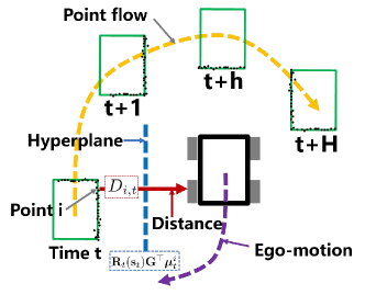
Figure 3: Point-to-distance mapping. $\mathbf{R}_{t}(\mathbf{s}_{t})\mathbf{G}^{\top}{\bm{\mu}_{t}^{i}}$ is the separation hyperplane between the point and ego robot. ${\bm{\mu}_{t}^{i}}^{\top}(\mathbf{G}{\mathbf{\widetilde{p}}_{t}^{i}(\mathbf{s}_{t})}-\mathbf{h})$ is equal to the exact distance.

IV-B Deep Unfolding

To guarantee collision avoidance at any time within the receding horizon of length $H$, it is necessary to compute the optimal $\{{\bm{\mu}_{t}^{i}}^{*}\}$ for any $t\in[t,t+H-1]$. Given the forward induction of the robot trajectory as $\mathcal{S}=\overline{\mathcal{S}}=\{\overline{\mathbf{s}}_{t},\cdots,\overline{\mathbf{s}}_{t+H-1}\}$ (obtained from last-frame solution or last-round iteration as mentioned in Section III), the space-time distance matrix $\mathbf{D}\in\mathbb{R}^{M\times H}$ is given by

$$\mathbf{D}=\left[{\begin{array}[]{*{20}{c}}{{\overline{D}_{{1,t}}}}&{{\overline{D}_{{1,t+1}}}}&{...}&{{\overline{D}_{{1,t+H-1}}}}\\ {{\overline{D}_{{2,t}}}}&{{\overline{D}_{{2,t+1}}}}&\cdots&{{\overline{D}_{{2,t+H-1}}}}\\ \vdots&\vdots&\ddots&\vdots\\ {{\overline{D}_{{M,t}}}}&{{\overline{D}_{{M,t+1}}}}&\ldots&{\overline{D}_{M,t+H-1}}\end{array}}\right],$$ (18)

where $\overline{D}_{i,t}=D_{i,t}(\mathbb{Z}_{t}(\overline{\mathbf{s}}_{t}),\mathbf{p}_{t}^{i})$. The inference mapping from points to distances for all points $\{i\}$ and time slots $\{t\}$ is thus to solve $M\times H$ problems in parallel, each having a similar formula as (10). This leads to a total computational complexity of $\mathcal{O}(MHl^{3.5})$ using off-the-shelf software, e.g., CVXPY, making it impossible for real-time applications, when $M$ is in the range of thousands or more.

To address the complexity issue while preserving interpretability, we propose a deep unfolding neural network to implement the point-distance mapping. The structure of this network is illustrated in Fig. 4, and its detailed derivation is given below.

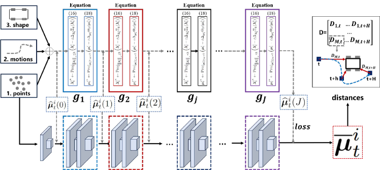
Figure 4: Structure of DUNE, which unfolds the PIBCD algorithm by imitating the labeled dataset generated by PIBCD. The trained DUNE is adopted for mapping points to $\bm{\mu}$-based distances in a real time.

IV-B1 Penalty Inexact Block Coordinate Descent

We use variable splitting and penalty method to reformulate (10). Penalizing (13), problem (10) is written as

$$\mathsf{Q}_{1}:\mathop{\min}\limits_{\bm{\mu}_{t}^{i},\bm{\lambda}_{t}^{i}}~{}C_{\mathsf{DUNE}}(\bm{\mu}_{t}^{i},\bm{\lambda}_{t}^{i}),~{}~{}\text{s.t.}~{}{\bm{\mu}_{t}^{i}}\succeq_{\mathcal{K^{*}}}0,~{}{\left\|\bm{\lambda}_{t}^{i}\right\|_{*}}\preceq 1,$$ (19)

in which

$$C_{\mathsf{DUNE}}(\bm{\mu}_{t}^{i},\bm{\lambda}_{t}^{i}) =-{\bm{\mu}_{t}^{i}}^{\top}(\mathbf{G}{{\mathbf{\widetilde{p}}_{t}^{i}}(\mathbf{\overline{s}}_{t})}-\mathbf{h})$$

$$+ \underbrace{\rho\|{\bm{\mu}_{t}^{i}}^{\top}\mathbf{G}+{\bm{\lambda}_{t}^{i}}^{\top}\mathbf{R}_{t}(\mathbf{\overline{s}}_{t})\|_{2}^{2}}_{\text{penalty~{}term}},$$ (20)

where $\rho$ is a sufficiently large penalty parameter, e.g., $\rho=10^{3}$, $\{\bm{\widetilde{\mu}}_{t}^{i},\bm{\widetilde{\lambda}}_{t}^{i}\}$ are solutions from the last iteration of NeuPAN. Due to strong convexity, (19) can be optimally solved via inexact block coordinate descent optimization, which updates $\bm{\mu}_{t}^{i}$ using gradient descent with $\bm{\lambda}_{t}^{i}$ fixed, and vice versa.

At the $j$-th iteration ($j$ is the counter for PIBCD), given the solution $\widehat{\bm{\mu}}_{t}^{i}(j-1)$ at the $(j-1)$-th iteration, the problem related to $\bm{\lambda}_{t}^{i}$ is

$$\mathop{\min}\limits_{\bm{\lambda}_{t}^{i}}~{}\Xi_{j}(\bm{\lambda}_{t}^{i}),~{}~{}\text{ s.t. }~{}{\left\|\bm{\lambda}_{t}^{i}\right\|_{*}}\preceq 1,$$ (21)

which is a quadratic minimization problem under norm ball constraints, with

$$\Xi_{j}(\bm{\lambda}_{t}^{i})={\|\widehat{\bm{\mu}}_{t}^{i}(j-1)}^{\top}\mathbf{G}+{\bm{\lambda}_{t}^{i}}^{\top}\mathbf{R}_{t}(\mathbf{\overline{s}}_{t})\|_{2}^{2}.$$

The associated one-step projected gradient descent update is

$${\bm{\lambda}_{t}^{i}}^{\star}\leftarrow\mathrm{Proj}_{{\left\|\bm{\lambda}_{t}^{i}\right\|_{*}}\preceq 1}\left({\bm{\lambda}_{t}^{i}}-\varepsilon\Delta_{\bm{\lambda}_{t}^{i}}\Xi_{j}(\bm{\lambda}_{t}^{i})\right),$$ (22)

where $\varepsilon$ is the step-size. With the updated ${\bm{\lambda}_{t}^{i}}^{\star}$, the problem related to $\bm{\mu}_{t}^{i}$ is

$$\mathop{\min}\limits_{\bm{\mu}_{t}^{i}}{}{} \Theta_{j}(\bm{\mu}_{t}^{i})$$ (23)

    s.t. $${\bm{\mu}_{t}^{i}}\succeq_{\mathcal{K^{*}}}0,$$

which is a quadratic minimization problem under box constraints, with

$$\Theta_{j}(\bm{\mu}_{t}^{i}) =\rho\|{\bm{\mu}_{t}^{i}}^{\top}\mathbf{G}+{{\bm{\lambda}_{t}^{i}}^{\star}}^{\top}\mathbf{R}_{t}(\mathbf{\overline{s}}_{t})\|_{2}^{2}$$

$$\quad{}{}-{\bm{\mu}_{t}^{i}}^{\top}(\mathbf{G}{{\mathbf{\widetilde{p}}_{t}^{i}}(\mathbf{\overline{s}}_{t})}-\mathbf{h}).$$

The associated one-step projected gradient descent update is

$${\bm{\mu}_{t}^{i}}^{\star}\leftarrow\mathrm{Proj}_{{\bm{\mu}_{t}^{i}}\succeq_{\mathcal{K^{*}}}0}\left({\bm{\mu}_{t}^{i}}-\varepsilon\Delta_{\bm{\mu}_{t}^{i}}\Theta_{j}(\bm{\mu}_{t}^{i})\right).$$ (24)

This completes one iteration. By setting $\widehat{\bm{\mu}}_{t}^{i}(j)={\bm{\mu}_{t}^{i}}^{\star}$, we can proceed to solve the problem for the $j$-th iteration. According to [41], the sequence $\{{\widehat{\bm{\mu}}_{t}^{i}(0)},{\widehat{\bm{\mu}}_{t}^{i}(1)},\cdots\}$ generated by the above iterative procedure is convergent, and converges to the optimal solution of (19) (thus (9)).

IV-B2 Deep Unfolding Neural Network

The sequence $\{{\widehat{\bm{\mu}}_{t}^{i}(0)},{\widehat{\bm{\mu}}_{t}^{i}(1)},\cdots\}$ generated by the PIBCD can be viewed as sequential mappings

$${\widehat{\bm{\mu}}_{t}^{i}(0)}\stackrel{{\scriptstyle g_{1}}}{{\longrightarrow}}{\widehat{\bm{\mu}}_{t}^{i}(1)}\stackrel{{\scriptstyle g_{2}}}{{\longrightarrow}}{\widehat{\bm{\mu}}_{t}^{i}(2)}\cdots\stackrel{{\scriptstyle g_{J}}}{{\longrightarrow}}{\widehat{\bm{\mu}}_{t}^{i}(J)}$$ (25)

These mappings $\{g_{1},g_{2},\cdots\}$ are all gradient mappings. More specifically, $g$ only consists of gradients of quadratic functions, which are matrix multiplication operations. Consequently, each $g_{i}$ can be safely unfolded into neural network layers that also correspond to matrix multiplications. The required number of iterations $J$ for PIBCD to converge determines the number of layers in the neural network. As such, deep unfolding takes a step towards interpretability by designing DNNs as learned variations of iterative optimization algorithms.

Based on the above observations, the architecture of the proposed DUNE is shown in Fig. 4. The first layer is the input layer with rectifier linear units (ReLUs), which reads the positions of $M\times H$ points in a batch manner from the point flow. After the input layer, there are $2J$ hidden layers (or blocks), each containing $128$ ReLUs. The final layer is the output linear layer followed by an activation function to generate the solution $\{{\overline{\bm{\mu}}}_{t}^{i}\}$. The entire network consist of $2J+2$ fully connected (FC) layers. As proved in [42, 43], $\{{\overline{\bm{\mu}}}_{t}^{i}\}$ is asymptotically optimal to (10) as $J$ goes to infinity. With $\{{\overline{\bm{\mu}}}_{t}^{i}\}$, the values of $\{{\overline{\bm{\lambda}}}_{t}^{i}\}$ is obtained using (13).

IV-B3 Loss function Design

The neural network is trained using a labeled dataset derived from the PIBCD algorithm. Back propagation is determined based on a loss function between the optimal solution, $\{\widehat{\bm{\mu}}_{t}^{i}\}$, and the neural network’s solution, $\{\overline{\bm{\mu}}_{t}^{i}\}$. A naive choice of the loss function is the mean square error (MSE) between these two values. However, since the learnt $\{\overline{\bm{\mu}}_{t}^{i}\}$ will be used in the subsequent motion planning as a regularizer for tackling the collision avoidance constraints, we must guarantee high accuracy of $\{\overline{\bm{\mu}}_{t}^{i}\}$ in different vector directions and incorporate non-Euclidean norms into the loss functions. Based on these considerations, we formulate the loss function as follows:

$$\mathcal{L}(\hat{\bm{\mu}_{i}},\overline{\bm{\mu}}_{i})=\|\bm{\widehat{\mu}_{i}}-\overline{\bm{\mu}}_{i}\|_{2}^{2}+\|f_{o}(\bm{\widehat{\mu}_{i}})-f_{o}(\overline{\bm{\mu}}_{i})\|_{2}^{2}$$ (26)

$$\quad\quad\quad+\|f_{a}(\bm{\widehat{\mu}_{i}})-f_{a}(\overline{\bm{\mu}}_{i})\|_{2}^{2}+\|f_{b}(\bm{\widehat{\mu}_{i}})-f_{b}(\overline{\bm{\mu}}_{i})\|_{2}^{2},$$

where, $f_{o}(\bm{\mu}_{i})={\bm{\mu}_{t}^{i}}^{\top}(\mathbf{G}{\mathbf{\widetilde{p}_{t}^{i}}}-\mathbf{h})$ is the objective function of problem (10). Functions $f_{a}(\bm{\mu}_{i})=-{\bm{\mu}_{i}}^{\top}\mathbf{G}\mathbf{R}_{t}^{\top}$ and $f_{b}(\bm{\mu}_{i})={\bm{\mu}_{i}}^{\top}\mathbf{G}\mathbf{R}_{t}^{\top}{\mathbf{\widetilde{p}_{t}^{i}}}-{\bm{\mu}_{i}}^{\top}\mathbf{h}$ are related to the kinematics constraints, which will be introduced in Section V.

(a) Box detection without error

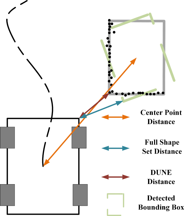
(b) Box detection with error

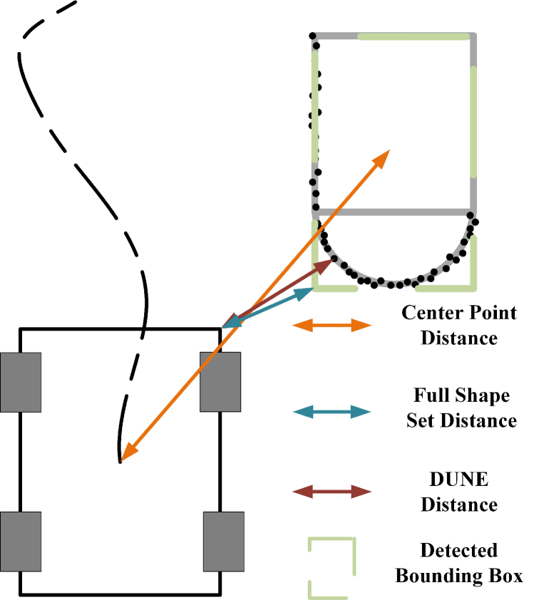
(c) Non-box convex objects

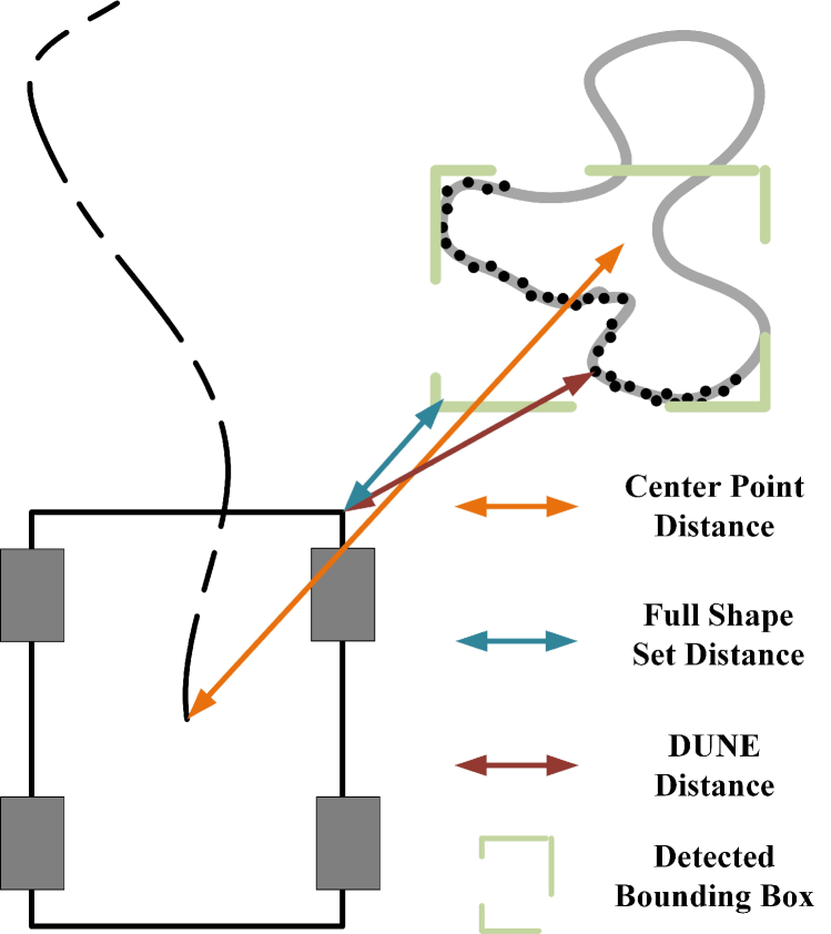
(d) Arbitrary shape objects

Figure 5: Intuitive comparison of DUNE distances, center point distances, and full shape set distances. DUNE distances are more accuracy than other distances.

IV-B4 Sim-to-Real Transfer

Collecting datasets for training DNNs in real-world environments is usually a challenge. In our case, however, we can train DUNE in the virtual environments, e.g., Carla [44], using simulated datasets. This is because 1) DUNE is obtained from deep unfolding, and 2) the point-distance mapping is unique and domain-invariant. To this end, for a robot with the given value $[\mathbf{G},\mathbf{h}]$, we use Carla to generate $N_{g}$ LiDAR points, with randomly generated objects within a specific range $[\mathbf{r}_{low},\mathbf{r}_{high}]$. Subsequently, $N_{g}$ problems with the form of (10) are constructed by $[\mathbf{G},\mathbf{h},\mathbf{\widetilde{p}}_{t}^{i}]$ and solved by the PIBCD algorithm, resulting in $N_{g}$ optimal values of $\widehat{\bm{\mu}}_{t}^{i}$. As such, each point position $\mathbf{\widetilde{p}}_{t}^{i}$ is one-to-one corresponding to each optimal solution of ${\bm{\mu}}_{t}^{i}$. This results in a labeled dataset $\mathcal{T}=\{\mathbf{\widetilde{p}}_{t}^{i},\widehat{\bm{\mu}}_{t}^{i}(j)\}$ for neural network training. In our experiment, the neural network is implemented using the PyTorch framework [45]. The training process is conducted on a desktop computer with an Intel Core i9 CPU and an NVIDIA GeForce GTX 4090Ti GPU. The training dataset consists of $N_{g}=10^{6}$ samples within the range $[\mathbf{r}_{l}=-50,\mathbf{r}_{h}=50]$. The training process is conducted for $10000$ epochs with a batch size of $32$. The Adam optimizer is leveraged to update the network parameters with a learning rate of $10^{-4}$ and decay rate of $0.9$. The training process takes approximately $2$ hours to complete.

1 Input: Robot shape $\{\mathbf{G},\mathbf{h}\}$ and LiDAR points in the ego-robot coordinate system ${\mathbf{\widetilde{p}}_{t}^{i}}(\mathbf{s}_{t})$ ;

2 Initialize: $\widehat{\bm{\mu}}_{t}^{i}(0)\succeq_{\mathcal{K^{*}}}0$;

3 for iteration $j=1,2,\cdots,J$ do

4       Compute ${\bm{\lambda}_{t}^{i}}^{\star}$ using (22);

5       Compute ${\bm{\mu}_{t}^{i}}^{\star}$ using (24);

6       Set $\widehat{\bm{\mu}}_{t}^{i}(j)={\bm{\mu}_{t}^{i}}^{\star}$ and $j\leftarrow j+1$.

7       if convergence then

8            break

9       end if

10      

11 end for

12Set training dataset $\mathcal{T}=\{\mathbf{\widetilde{p}}_{t}^{i},\hat{\bm{\mu}}_{t}^{i}(J)\}$;

13 for epoch $e=1,2,\cdots,E$ do

14       Calculate the loss function (26);

15       Back propagation using $\mathcal{T}$;

16       if  loss converges  then

17            break

18       end if

19      

20 end for

Output: DUNE model.

Algorithm 1 Deep Unfolded Neural Encoder

IV-C Comparison with Other Distances

To demonstrate the high-accuracy property of DUNE, we compare the exact distances generated by DUNE and inexact distances generated by other existing approaches. An intuitive comparison is illustrated in Fig. 5. It can be seen that the center point distance has the lowest accuracy, since it does not take the object shape into account. The full shape set distance is accurate if and only if the object has a box shape and the detector is $100\,\%$ accurate as shown in Fig. 5(a). Otherwise, the set distance would involve non-negligible distance errors as shown in Fig. 5(b) (if the detector is inaccurate) and Fig. 5(c) (if the shape is not a box). Lastly, the proposed DUNE can handle arbitrary nonconvex shapes as shown in Fig. 5(d), whereas all other approaches break down.

V Neural Regularized Motion Planner

This section presents NRMP, which corresponds to solving the proximal version of $\mathcal{Q}$ with $\{\mathcal{M},\mathcal{L}\}$ fixed to $\{\mathcal{M}=\overline{\mathcal{M}},\mathcal{L}=\overline{\mathcal{L}}\}$, where $\overline{\mathcal{M}}=\{{\overline{\bm{\mu}}}_{t}^{i}\}$ and $\overline{\mathcal{L}}=\{{\overline{\bm{\lambda}}}_{t}^{i}\}$ are generated from the upstream DUNE. This leads to the following problem

$$\mathsf{Q}_{2}:\min_{\begin{subarray}{c}\{\mathcal{S},\mathcal{U}\}\in\mathcal{F}\end{subarray}}~{} C_{0}(\mathcal{S},\mathcal{U})+\underbrace{C_{r}(\mathcal{S},\overline{\mathcal{M}},\overline{\mathcal{L}})}_{\text{neural~{}regularizer}}$$

$$+\underbrace{\frac{b_{k}}{2}\sum_{h=0}^{H-1}\|\mathbf{s}_{t+h}-\mathbf{\overline{s}}_{t+h}\|_{2}^{2}}_{\text{proximal~{}term}},$$ (27)

where $\overline{\mathbf{s}}$ is short for $\mathbf{s}^{[k-1]}$ obtained from last iteration of NeuPAN, and $b_{k}$ is the associated proximal coefficient at NeuPAN iteration $k$. This subproblem aims to convert distances to collision-free robot actions. But to solve it, we need to determine: 1) the constraint $\{\mathcal{S},\mathcal{U}\}\in\mathcal{F}$ for explicitly incorporating physical robot dynamics using MPC; and 2) the analytical form of regularizer $C_{r}$. Then, we need to convert the planner into a learnable optimization network that can learn from failures in both online and offline manners and adjust its parameters (e.g., trade-off between path following and collision avoidance).

V-A MPC Model

The dynamics set $\mathcal{F}$ contains two parts: 1) physical boundary; and 2) state evolution. The first part is straightforward, i.e., we can directly set lower and upper bounds on the absolute values (i.e., $\{\mathbf{u}_{\text{min}},\mathbf{u}_{\text{max}}\}$) and rates of changes (i.e., $\{\mathbf{a}_{\text{min}},\mathbf{a}_{\text{max}}\}$) on the control vector $\mathbf{u}_{t}$. This yields the following equations:

$$\mathbf{u}_{\text{min}}\preceq\mathbf{u}_{t+h}\preceq\mathbf{u}_{\text{max}},~{}\mathbf{a}_{\text{min}}\preceq\mathbf{u}_{t+h+1}-\mathbf{u}_{t+h}\preceq\mathbf{a}_{\text{max}},\quad\forall h.$$

Now the remaining question is how to model the state evolution for producing physically-reasonable trajectories. In particular, the current and subsequent states of the robot, denoted by $\mathbf{s}_{t}$ and $\mathbf{s}_{t+1}$ respectively, must adhere to the discrete-time kinematic constraints $f({\mathbf{s}_{t}},{\mathbf{u}_{t}})$ with the control vector $\mathbf{u}_{t}$, as encapsulated by the following equation:

$${\mathbf{s}_{t+1}}={\mathbf{s}_{t}}+f({\mathbf{s}_{t}},{\mathbf{u}_{t}})\Delta t,$$ (28)

where $\Delta t$ is the time slot between two states. We assume that the function $f({\mathbf{s}_{t}},{\mathbf{u}_{t}})$ is linear with respect to the state ${\mathbf{s}_{t}}$ and control vector $\mathbf{u}_{t}$. In scenarios involving non-linear dynamics, these functions can be approximated using linearization techniques, such as the Taylor series expansion. Accordingly, this constraint can be rewritten in a linear form:

$${\mathbf{s}_{t+1}}=\mathbf{A}_{t}{\mathbf{s}_{t}}+\mathbf{B}_{t}{\mathbf{u}_{t}}+{\mathbf{c}_{t}},$$ (29)

where $(\mathbf{A}_{t},\mathbf{B}_{t},\mathbf{c}_{t})$ are coefficient matrices at time step $t$. Examples for ackermann and differential models are provided in Appendix B (detailed in the supporting document).

V-B Neural Regularizer

The proposed regularization function is

$$C_{r}(\mathcal{S},\mathcal{M},\mathcal{L}) =\frac{\rho_{1}}{2}\sum_{h=0}^{H-1}\sum_{i=0}^{M^{\prime}}\left\|\min(I(\mathbf{s}_{t+h},{{\bm{{\mu}}}}_{t+h}^{i},{\bm{\lambda}}_{t+h}^{i}),0)\right\|_{2}^{2}$$

$$\quad+\frac{\rho_{2}}{2}\sum_{h=0}^{H-1}\sum_{i=0}^{M^{\prime}}\left\|H(\mathbf{s}_{t+h},{{\bm{{\mu}}}}_{t+h}^{i},{\bm{\lambda}}_{t+h}^{i})\right\|_{2}^{2},$$

and the penalty functions $I$ and $H$ are

$$I(\mathbf{s}_{t},{{\bm{{\mu}}}}_{t}^{i},{\bm{\lambda}}_{t}^{i}) ={\bm{\lambda}_{t}^{i}}^{\top}(\mathbf{t}_{t}(\mathbf{s}_{t})-\mathbf{p_{t}}^{i})-{\bm{{\mu}}_{t}^{i}}^{\top}\mathbf{h}-d_{\mathrm{min}},$$ (30)

$$H(\mathbf{s}_{t},{{\bm{{\mu}}}}_{t}^{i},{\bm{\lambda}}_{t}^{i}) ={\bm{{\mu}}_{t}^{i}}^{\top}\mathbf{G}+{\bm{\lambda}_{t}^{i}}^{\top}\mathbf{R}(\mathbf{s}_{t}).$$ (31)

In particular, $C_{r}$ has the following properties:

• $C_{r}$ is a nonlinear but convex function of $\{\mathbf{s}_{t}\}$.

• $C_{r}$ is a function of $\mathcal{M}=\{{\bm{\mu}}_{t}^{i}\}$ and $\mathcal{L}=\{{\bm{\lambda}}_{t}^{i}\}$, which conditions on $\overline{\mathcal{M}}=\{{\overline{\bm{\mu}}}_{t}^{i}\}$ and $\overline{\mathcal{L}}=\{{\overline{\bm{\lambda}}}_{t}^{i}\}$ generated from the upstream neural encoder. That is why we call $C_{r}$ “neural regularizer”.

• $C_{r}$ guarantees the equivalence between problems $\mathsf{P}$ and $\mathsf{Q}$ if $\rho_{1},\rho_{2}\rightarrow\infty$ as shown in Appendix A.

• In practice, we cannot set $\rho_{1},\rho_{2}\rightarrow\infty$ to ensure the smoothness of $C_{r}$. Hence, coefficients $\rho_{1}$ and $\rho_{2}$ need to be carefully tuned to control the trade-off between the smoothness of $C_{r}$ and the gap from $\mathsf{P}$ to $\mathsf{Q}$.

Problem $\mathsf{Q}_{2}$ is a convex optimization program due to: 1) convexity of norm function $C_{0}$ in (2); 2) linearity of $\mathcal{F}$; and 3) property (i) of $C_{r}$. Consequently, $\mathsf{Q}_{2}$ can be optimally solved via the off-the-shelf software for solving convex problems, e.g., cvxpy. However, this would involve manually tuning parameters $\{\mathbf{q},\mathbf{p},d_{\mathrm{min}}\}$ in $C_{0}$ and $C_{r}$. To address this issue, the next subsection will derive a learnable optimization method to update $\mathcal{P}$ automatically.

V-C Learnable Optimization Network

In order to enable automatic calibration of parameters in $\mathsf{Q}_{2}$ under new environments, we present a learnable optimization network (LON) approach for solving $\mathsf{Q}_{2}$. The crux to LON is that it leverages differentiable convex optimization layers (cvxpylayers) [46]. As such, in contrast to traditional optimization solvers, LON offers the ability to differentiate through disciplined convex programs. Within these programs, parameters can be mapped directly to solutions, facilitating back-propagation calculations. Moreover, with cvxpylayers, the NRMP can be seamlessly integrates with the DUNE, as both of them supports back propagation, thereby enabling end-to-end training of the entire NeuPAN system.

However, solving $\mathsf{Q}_{2}$ using LON is nontrivial, since cvxpylayers require the optimization problem to satisfy disciplined parametrized program (DPP) form. To this end, this paper proposes the following problem reconfiguration that recasts $\mathsf{Q}_{2}$ into a DPP-friendly problem. In particular, to satisfy the DPP formats in [46], we reconfigure the non-DPP function $C_{0}$ by introducing a set of DPP variables $\{^{a}\!\bm{\gamma}_{t}^{i},^{b}\!\bm{\gamma}_{t}^{i}\}$, which gives

$$C_{0}^{\text{DPP}}(\mathcal{S},\mathcal{U})= \sum_{h=0}^{H-1}\Bigg{(}\left\|\mathbf{q}\circ{{\mathbf{s}_{t+h}}-^{a}\!\bm{\gamma}_{t+h}^{i}}\right\|_{2}^{2}$$

$$\quad\quad+\left\|\mathbf{p}\circ\mathbf{u}_{t+h}-^{b}\!\bm{\gamma}_{t+h}^{i}\right\|_{2}^{2}\Bigg{)},$$ (32)

where ${}^{a}\!\bm{\gamma}_{t+h}^{i}\leftarrow\mathbf{q}\circ{\mathbf{s}_{t+h}}^{\diamond}$ and ${}^{b}\!\bm{\gamma}_{t+h}^{i}\leftarrow\mathbf{p}\circ\mathbf{u}_{t+h}^{\diamond}$ are introduced as learnable parameters for back propagation. On the other hand, we reformulate $C_{r}$ in $\mathsf{Q}_{2}$ as

$$C_{r}^{\text{DPP}}(\mathcal{S},\mathcal{U},\mathcal{L})$$

$$=\frac{\rho_{1}}{2}\sum_{h=0}^{H-1}\sum_{i=0}^{M}\left\|\min(I^{\text{DPP}}(\mathbf{s}_{t+h},{{\bm{{\mu}}}}_{t+h}^{i},{\bm{\lambda}}_{t+h}^{i}),0)\right\|_{2}^{2}$$

$$\quad+\frac{\rho_{2}}{2}\sum_{h=0}^{H-1}\sum_{i=0}^{M}\left\|H^{\text{DPP}}(\mathbf{s}_{t+h},{{\bm{{\mu}}}}_{t+h}^{i},{\bm{\lambda}}_{t+h}^{i})\right\|_{2}^{2},$$ (33)

where the DPP-reformulated $I$ and $H$ are

$$I^{\text{DPP}} =^{c}\!\bm{\gamma}_{t}^{i}\mathbf{t}_{t}(\mathbf{s}_{t})-^{a}\!\xi_{t}^{i}-^{b}\!\xi_{t}^{i},$$ (34)

$$H^{\text{DPP}} =^{d}\!\bm{\gamma}_{t}^{i}+^{c}\!\bm{\gamma}_{t}^{i}\mathbf{R}_{t}(\mathbf{s}_{t}),$$ (35)

with vector ${}^{c}\!\bm{\gamma}_{t}^{i}\leftarrow{\bm{\lambda}_{t}^{i}}^{\top},^{d}\!\bm{\gamma}_{t}^{i}\leftarrow{\bm{\mu}_{t}^{i}}^{\top}\mathbf{G}$, and scalar ${}^{a}\!\xi_{t}^{i}\leftarrow{\bm{\lambda}_{t}^{i}}^{\top}\mathbf{p}_{t}^{i}+{\bm{\mu}_{t}^{i}}^{\top}\mathbf{h},^{d}\!\xi_{t}^{i}\leftarrow d_{\mathrm{min}}$. The learnable parameters are

$$\mathcal{P}=\{^{a}\!\bm{\gamma}_{t}^{i},^{b}\!\bm{\gamma}_{t}^{i},^{c}\!\bm{\gamma}_{t}^{i},^{d}\!\bm{\gamma}_{t}^{i},^{a}\!\xi_{t}^{i},^{b}\!\xi_{t}^{i}\}.$$ (36)

With the above reconfiguration, problem $\mathsf{Q}_{2}$ becomes

$$\mathsf{Q}_{2}^{\text{DPP}}:\min_{\begin{subarray}{c}\{\mathcal{S},\mathcal{U}\}\in\mathcal{F}\end{subarray}}~{} C_{0}^{\text{DPP}}(\mathcal{S},\mathcal{U})+C_{r}^{\text{DPP}}(\mathcal{S},\overline{\mathcal{M}},\overline{\mathcal{L}})$$

$$+\frac{b_{k}}{2}\sum_{h=0}^{H-1}\|\mathbf{s}_{t+h}-\mathbf{\overline{s}}_{t+h}\|_{2}^{2}.$$ (37)

It can be proved that both $C_{0}$ and $C_{r}$ satisfy the DPP regulation. Adding to the fact that other functions in set $\mathcal{F}$ are DPP-friendly, problem $\mathsf{Q}_{2}^{\text{DPP}}$ is DPP compatible, whose variables and parameters can be optimized using the back propagation. Specifically, a parameter, say $x\in\mathcal{P}$, can be revised utilizing the gradient descent method, facilitated by a loss function $L(\mathcal{P})$, as follows:

$$x^{(k+1)}=x^{(k)}-\alpha\frac{\partial{L}}{\partial x}$$ (38)

where, $\alpha$ is the learning rate. The gradient is clipped in a range $[g_{\text{min}},g_{\text{max}}]$, with the maximum value of $1.0$ to avoid the gradient explosion.

The loss function $L(\mathcal{P})$ is designed based on the cost function $C_{0}+C_{r}$ presented in $\mathsf{Q}_{2}$. The key idea is to allow the LON to learn from failures. Such failure situations consist of three cases: (i) Colliding with obstacles; (ii) Getting stuck in a congested environment; (iii) Straying from the destination. Based on this observation, we design the following cost functions to train LON:

$$\left\{\begin{aligned} L_{1}(\mathcal{P})&=\|{\mathbf{s}}(\mathcal{P})-\mathbf{s}^{\diamond}\|_{2}^{2},\\ L_{2}(\mathcal{P})&=\|{\mathbf{u}}(\mathcal{P})-\mathbf{u}^{\diamond}\|_{2}^{2}+\|{d_{\mathrm{min}}}(\mathcal{P})\|_{1},\\ L_{3}(\mathcal{P})&=-\|{\mathbf{s}}(\mathcal{P})-\mathbf{s}^{\diamond}\|_{2}^{2}-\|{d_{\mathrm{min}}}(\mathcal{P})\|_{1},\end{aligned}\right.$$

Now we consider three failure cases.

• If the robot strays from the destination, the learning problem is $\min\,L_{1}(\mathcal{P})$, which yields a larger $\mathbf{q}$, and forces the robot return to the correct path. This case is implemented as a function $\mathsf{RobotStray}(\cdot)$ in ROS.

• If the robot gets stuck in a congested environment, the learning problem is $\min\,L_{2}(\mathcal{P})$, which yields a larger $\mathbf{q}$ but a smaller $d_{\mathrm{min}}$ that creates an incentive for robot motion. This case is implemented as a function $\mathsf{RobotStuck}(\cdot)$ in ROS.

• If the robot collides with obstacles, the learning problem is $\min\,L_{3}(\mathcal{P})$, which yields a smaller $\mathbf{q}$ allowing the robot to temporarily leave from the reference path, and a larger $d_{\mathrm{min}}$ producing more conservative movements. This case is implemented as a function $\mathsf{RobotCollision}(\cdot)$ in ROS.

The entire procedure is summarized in Algorithm 2.

1 Input: Latent variables $\{\mathcal{\overline{M}},\mathcal{\overline{L}}\}$ from DUNE;

2    Robot Geometry information $[\mathbf{G},\mathbf{h}]$;

3 Construct parametrized convex optimization problem;

4 Initialize the parameters $\mathcal{P}=\{^{a}\!\bm{\gamma}_{t}^{i},^{b}\!\bm{\gamma}_{t}^{i},^{c}\!\bm{\gamma}_{t}^{i},^{d}\!\bm{\gamma}_{t}^{i},^{a}\!\xi_{t}^{i},^{b}\!\xi_{t}^{i}\}$ manually by using $\{\mathbf{G},\mathbf{h}\}$ and $\{\mathcal{\overline{M}},\mathcal{\overline{L}}\}$;

5 Solve the problem (37) via DPP solver;

6 if  $\mathsf{RobotStray(\cdot)}$ returns True  then

7      Update NRMP via back propagation by cost $L_{1}$

8 end if

9if  $\mathsf{RobotStuck}(\cdot)$ returns True  then

10      Update NRMP via back propagation by cost $L_{2}$

11 end if

12if  $\mathsf{RobotCollision}(\cdot)$ returns True then

13      Update NRMP via back propagation by cost $L_{3}$

14 end if

Output: State and action sequence $[\mathcal{S},\mathcal{U}]$.

Algorithm 2 DPP-based NRMP

V-D Dynamic Safety Distance Regularizer

In practice, a static safety distance $d_{\mathrm{min}}$ may not be suitable for time-varying environments. As a consequence, $d_{\mathrm{min}}$ in $\mathsf{Q}_{2}^{\text{DPP}}$ needs to be dynamically adjusted. To achieve this goal, we propose to use a variable distance $d_{t}$ to replace $d_{\mathrm{min}}$ in $I^{\text{DPP}}$, where $d_{t}$ is within the range $[{d_{\min}},{d_{\max}}]$. To encourage $d_{t}$ to approach $d_{\min}$ in highly-confined spaces and to approach $d_{\max}$ in highly-dynamic environments, we propose a sparsity-induced distance regularizer $C_{1}(\mathbf{d})=-\eta\sum_{h=0}^{T}\|\mathbf{d}_{t+h}\|_{1}$, where $\eta$ is a weighting factor. As such, $C_{1}(\mathbf{d})$ introduces adaptation to collision [21]. In this case, parameters $d_{\max}$ and $\eta$ are added into $\mathcal{P}$ for online updating, and ${d_{\mathrm{min}}}(\mathcal{P})$ in (V-C) is replaced by $C_{1}$.

VI Convergence and Complexity Analysis

Based on DUNE and NRMP algorithms in Sections IV and V, the entire procedure of NeuPAN is summarized in Algorithm 3. To see why NeuPAN works, the following theorem is established.

1 Input: Robot geometry information $[\mathbf{G},\mathbf{h}]$;

2    Current robot states $\mathbf{s}_{t}$;

3    Current point cloud $\mathbb{P}_{t}$;

4    Well-trained neural encoder DUNE;

5    Parametrized optimization network NRMP;

6

7Initialize $\mathcal{S}^{[0]}$ and $\mathcal{U}^{[0]}$.

8for iteration $k=0,1,2,\cdots$ do

9       Generate point flow $\mathbb{PF}$ from the current scan $\mathbb{P}_{t}$ and robot states $\mathcal{S}^{[k]}$;

10       Generate the latent distance features $\{\overline{\mathcal{M}},\overline{\mathcal{L}}\}$ via DUNE;

11       Generate the state-action variables $\{\overline{\mathcal{S}},\overline{\mathcal{U}}\}$ via NRMP;

12       Update $\{\mathcal{M}^{[k+1]}=\overline{\mathcal{M}},\mathcal{L}^{[k+1]}=\overline{\mathcal{L}}\}$;

13       Update $\{\mathcal{S}^{[k+1]}=\overline{\mathcal{S}},\mathcal{U}^{[k+1]}=\overline{\mathcal{U}}\}$;

14      

15      if stopping criterions are satisfied, then

16             break;

17            

18       end if

19      Update $k\leftarrow k+1$;

20 end for

21

Output: Control vector $\mathbf{u}_{t}$.

Algorithm 3 NeuPAN

Theorem 1.

The sequence $\left[\{\mathcal{S}^{[0]},\mathcal{U}^{[0]}\},\{\mathcal{S}^{[1]},\mathcal{U}^{[1]}\},\cdots\right]$ satisfies the following conditions:

(i) Monotonicity: $C_{\mathrm{e2e}}^{[0]}\geq C_{\mathrm{e2e}}^{[1]}\geq C_{\mathrm{e2e}}^{[2]}\geq\cdots,$ where $C_{\mathrm{e2e}}^{[k]}=C_{\mathrm{e2e}}(\mathcal{S}^{[k]},\mathcal{U}^{[k]},\mathcal{M}^{[k]},\mathcal{L}^{[k]})$.

(ii) Convergence: $\|C_{\mathrm{e2e}}^{[k+1]}-C_{\mathrm{e2e}}^{[k]}\|_{2}\rightarrow 0$ as $k\rightarrow\infty$.

(iii) Convergence to a critical point of $\mathsf{Q}$.

Proof.

See Appendix C (detailed in the supporting document). ∎

Part (i) of Theorem 1 states that adding the tightly-coupled feedback from the NRMP (i.e., locomotion) to the DUNE (i.e., perception) is guaranteed to improve the performance of the NeuPAN system (under the criterion of solving $\mathsf{P}$). Part (ii) of Theorem 1 means that we can safely iterate the loop, since the outputs converge and do not explode. Part (iii) of Theorem 1 implies that the states and actions generated by NeuPAN must be at least a local optimal solution to $\mathsf{Q}$, which is an equivalent problem to $\mathsf{P}$. All the above insights indicate that the proposed algorithm has end-to-end mathematical guarantee, which is in contrast to all existing approaches.

Based on Theorem 1, we can terminate NeuPAN until convergence. In practice, to save the computation time and enable real-time end-to-end robot navigation, we terminate the NeuPAN iteration when the number of iterations reach the limit, e.g., $K=3$.

Finally, we present the complexity analysis of NeuPAN. Depending on the procedure listed in Algorithm 3, in each iteration, the scan flow is first generated from the scan data with a complexity of $\mathcal{O}(MH)$. Subsequently, DUNE consists of multiple neural layers at a computational cost of $\mathcal{O}(MHN_{n})$, where $N_{n}$ is the number of neurons in the DUNE neural network. Next is the NRMP, which solves a DPP based optimization problem with a complexity of $\mathcal{O}(H(n+2))^{3.5}$. In summary, with the number of iterations required to converge being $K$, the total complexity of NeuPAN is $\mathcal{O}(K(MH(N_{n}+1)+(H(n+2))^{3.5}))$. It can be seen that the complexity is linear with $M$ which corroborates to the facts that NeuPAN can tackle thousands of points in real-time.

VII Numerical Simulation

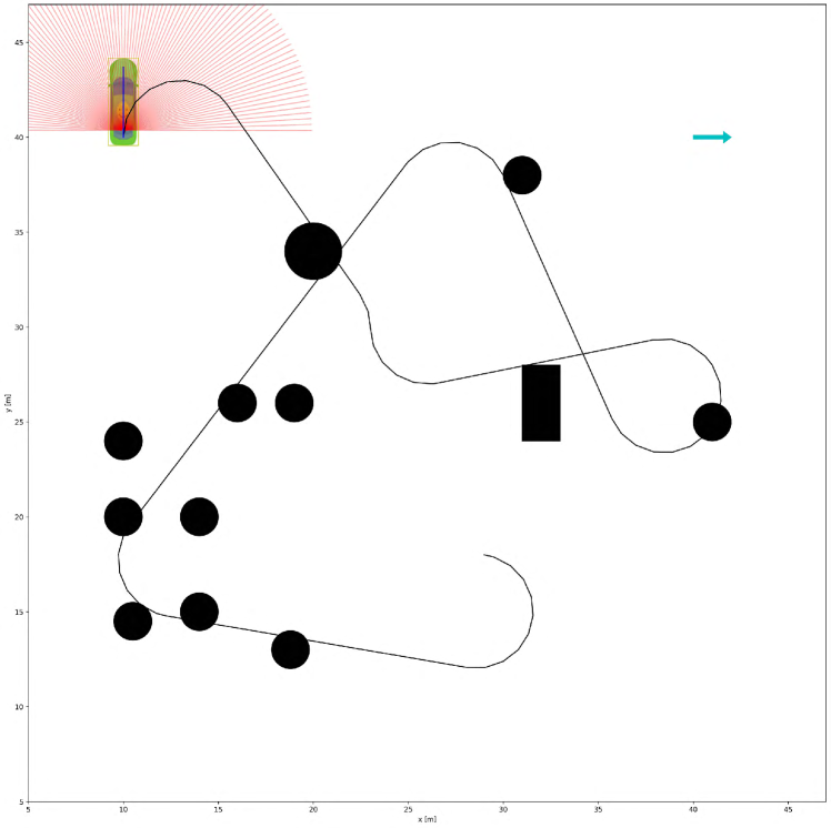
(a) RDA at time step 0

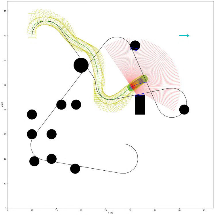
(b) RDA at time step 93

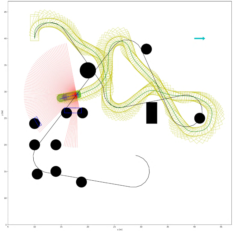
(c) RDA at time step 241

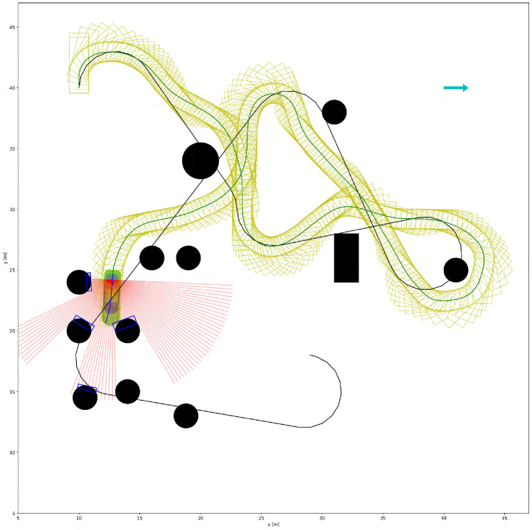
(d) RDA gets stuck

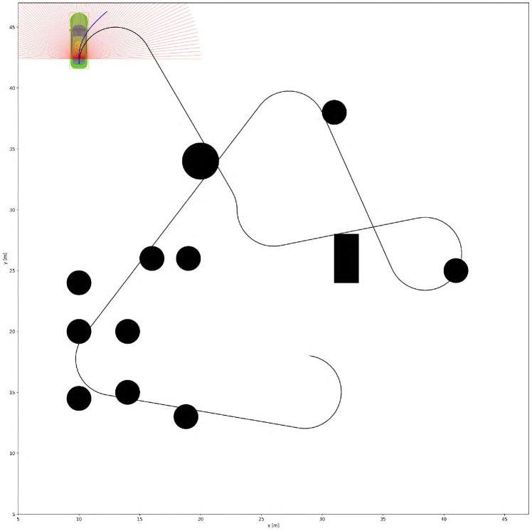
(e) NeuPAN at time step 0

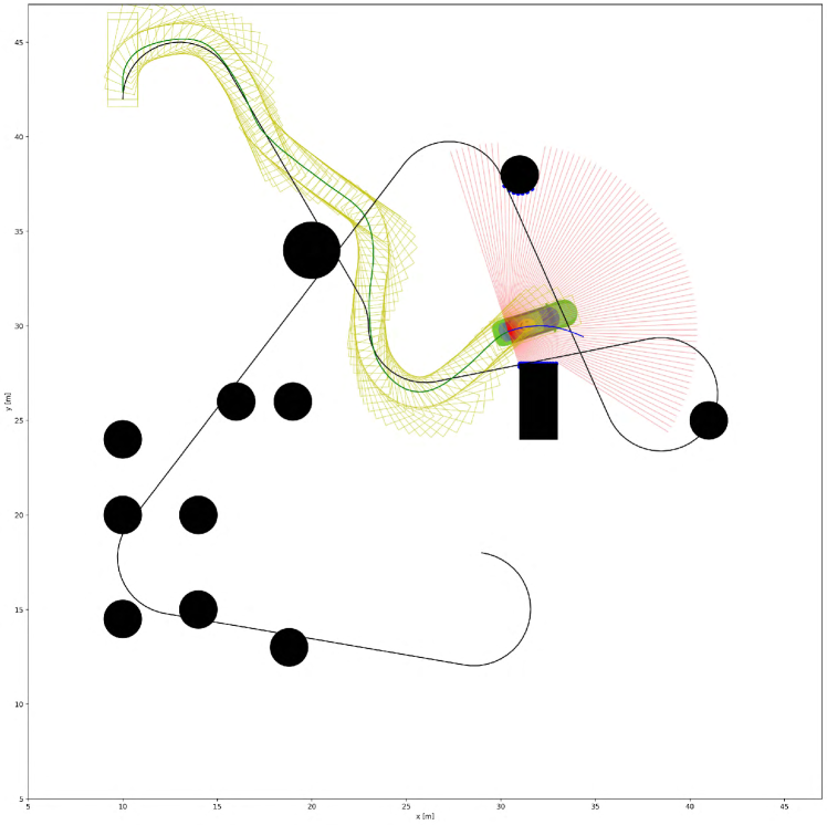
(f) NeuPAN at time step 93

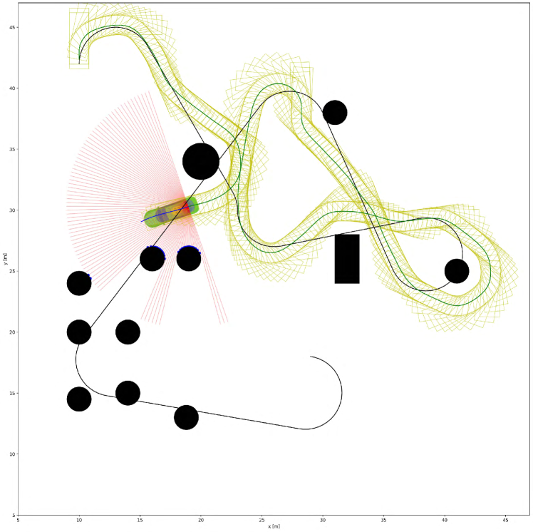
(g) NeuPAN at time step 241

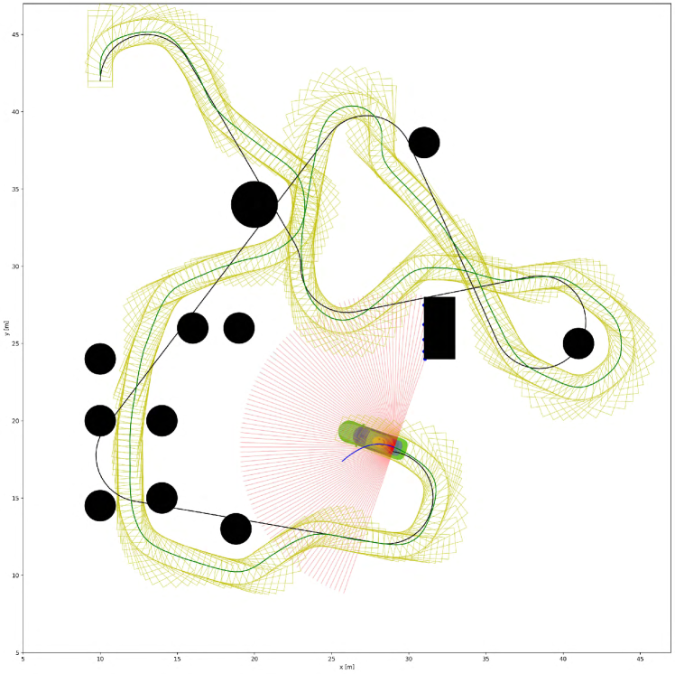
(h) NeuPAN learns from failure

Figure 6: Navigation process and trajectory comparison of NeuPAN and RDA planner in the path following scenario. The robot is required to plan a trajectory (blue line) to follow the reference path (black line) avoiding the cluttered obstacles (black circle). RDA require the detection algorithm to convert the LiDAR scan to the convex objects (blue rectangle).

This section presents numerical results in our self-developed Python-based 2D robot simulator, ir-sim, to analyze the effectiveness, efficiency, and trajectory quality of NeuPAN.

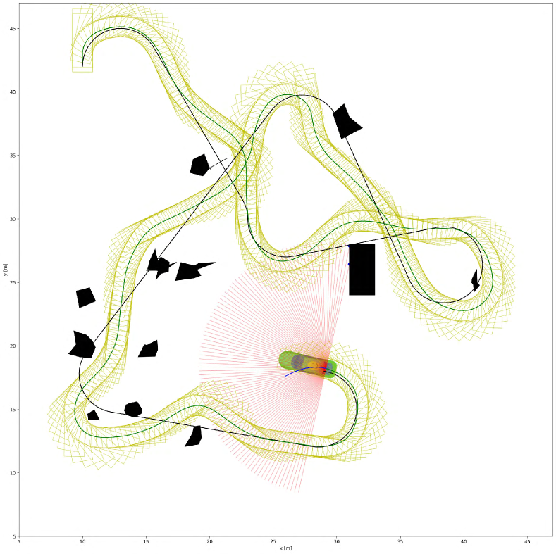
(a) Ackermann robot avoids non-convex obstacles.

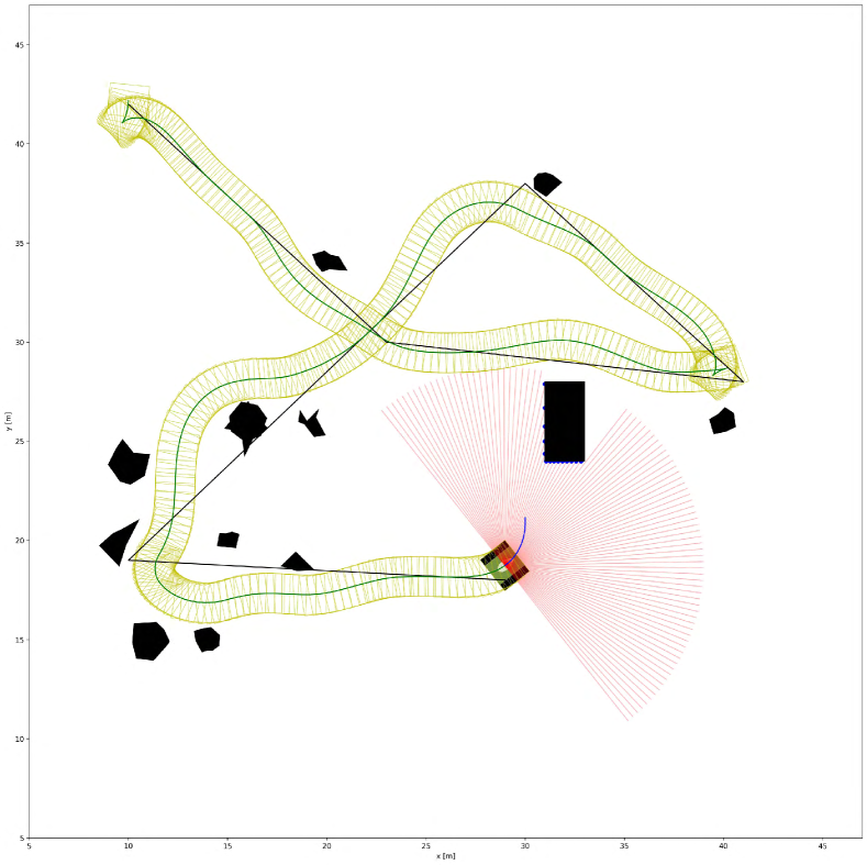
(b) Differential robot avoids non-convex obstacles.

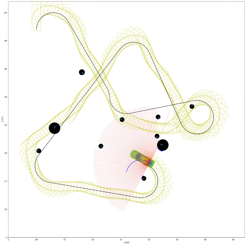
(c) Ackermann robot avoids dynamic objects.

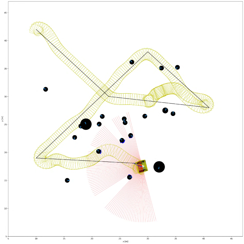
(d) Differential robot avoids dynamic objects.

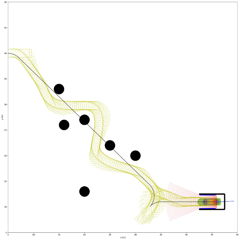
(e) Ackermann robot for automated reverse parking.

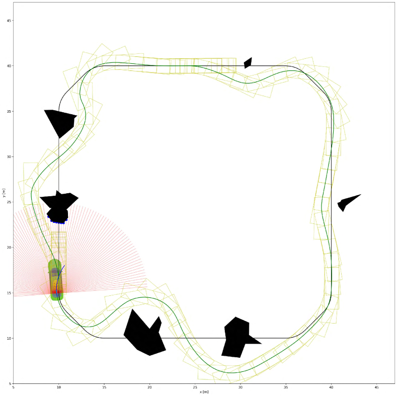
(f) Ackermann robot with online updating for new environments.

Figure 7: Verification of NeuPAN in various scenarios on two types of robots.

VII-A Path Following

In this scenario, the robot needs to follow a predefined route full of cluttered obstacles, as depicted in Fig. 6 (a). A car-like rectangular robot equipped with a 2D 100-line LiDAR sensor is considered. We compare the proposed method with a SOTA modular approach consisting of a perfect object detector and a full shape optimization-based planner, RDA [21]. The trajectories obtained from the benchmark and the NeuPAN at different frames are shown in Fig. 6(a)-(d) and Fig. 6(e)-(h), respectively. It can be seen that both schemes are capable of maneuvering the robot in open spaces with sparsely distributed obstacles. However, since the benchmark scheme needs to transform laser scans into boxes or convex sets using object detection (as shown in Fig. 6(c)), errors are inevitably introduced between the detection results and the actual objects. As a consequence, even under ideal LiDAR and detector in the considered experiment, the modular approach may still result in collisions in densely cluttered environments (as shown in Fig. 6(d)). In contrast, the proposed NeuPAN directly processes the points, thus bypassing intermediate steps, resulting in a more accurate navigation performance in cluttered scenarios.

VII-B Nonconvex, Dynamic, and Parking Scenarios

To illustrate the comprehensiveness of NeuPAN, we conduct experiments in diverse scenarios using two different robot models: the car-like robot (Ackermann) and the differential-drive robot. These models are widely used in practice and adhere to different kinematic constraints. The target scenarios and robot trajectories are depicted in Fig. 7. First, Fig. 7(a) and Fig. 7(b) demonstrate the capability of NeuPAN passing through marginal gaps between nonconvex obstacles. To date, nonconvex obstacles pose a significant challenge for existing optimization-based approaches [3, 21]. Approximating these non-convex objects as convex forms would lead to inaccurate representations and dividing them into a group of convex sets would lead to high computation costs. In contrast, the proposed direct point approach efficiently address these complex, non-convex, and unstructured obstacles. Second, the validation of NeuPAN in dynamic collision avoidance scenarios is illustrated in Figs. 7(c) and 7(d). Finally, the verification of NeuPAN in the reverse parking scenario is presented in Fig. 7(e). These results demonstrate the comprehensiveness and generalizability of our NeuPAN system, which corroborate Table I.

VII-C Online Parameter Fine-tuning

Fig. 7(f) presents the result for online parameter fine-tuning of NRMP using LON. In particular, at the beginning, the robot struggles with avoiding dense obstacles due to inappropriate parameters. However, after updating these parameters using end-to-end back propagation with failure data, the robot gradually evolves and eventually successfully moves through the narrow gaps. This corroborates the theory in Section V-C and demonstrates the adaptiveness nature of our approach. Note that for a fixed robot platform, there is no need to retrain DUNE, and we only need to adjust a few parameters involved in NRMP, which results in a fast online learning procedure. In contrast, the learning based end-to-end approaches [9, 25] require model retraining for new environments. On the other hand, for a new robot platform, we also need to retrain DUNE, but this process only takes hour-level time. This is significantly more efficient compared to other methods which may requires days of training, as reported in [9, 25].

VII-D Computation Time

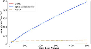
Figure 8: Computational time analysis of our approach with varying number of input points.

Time efficiency is crucial for real-time applications. The computation time of DUNE and NRMP versus the number of LiDAR points is shown in Fig. 8. The tests were performed on a Intel x86 computer equipped with an i7-9700 CPU. Our findings imply that the computation time of DUNE is reduced by orders of magnitude compared to the optimization software. On the other hand, NRMP achieves a computation time of below $50\,$ms (i.e., $20\,$Hz) when the number of point-level regularizers in the range of hundreds or more. The time efficiencies of DUNE and NRMP make NeuPAN sufficiently agile for real-time applications, thus suitable for tackling dynamic environments.

VIII Experiments

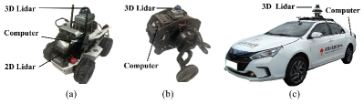
Figure 9: Experimental platform with different types of robots. (a) Ground mobile robot. (b) Wheel-legged robot. (c) Autonomous driving vehicle.

This section validates the performance of NeuPAN on different robot platforms based on high-fidelity simulations and real-world test tracks under the real-world settings. The considered robot platforms include the agile mobile robot, wheel-legged robot, and passenger autonomous vehicle, as depicted in Fig. 9. The agile mobile robot shown in Fig. 9(a) is a customized, multi-modal, small-size robot platform, whose steering modes can be switched between the differential and Ackermann modes. The wheel-legged robot shown in Fig. 9(b) is a middle-size platform that integrates the functionalities of both wheeled and legged robots, thus enjoying the joint benefits of high-mobility and terrain-adaptability in complex scenarios. Different from the agile robot in Fig. 9(a), wheel-legged robot is prone to oscillation, which requires much more precise motions for guaranteeing stability. The passenger autonomous vehicle shown in Fig. 9(c) is a $4.675\,\mathrm{m}\times 1.77\,\mathrm{m}\times 1.5\,\mathrm{m}$ large-size platform for urban driving. All these platforms are equipped with LiDAR systems (2D or 3D), enabling them to obtain the points representation of the environment. Localization of these robots in unknown environments is realized by Fast-lio [47] and lego-loam [48]. All the experiments are conducted without any prior map, relying solely on the onboard LiDAR for navigation and exploration.

To quantify the level of navigation difficulty in cluttered environments, we define a metric termed Degree of Narrowness (DoN), as follows:

$$\mathsf{DoN}=\frac{\mathrm{robot~{}width}}{\mathrm{minimum~{}passable~{}space~{}width}}$$ (39)

Higher DoN (closer to 1) means a narrower space and a higher difficulty for robot navigation; and vice versa.

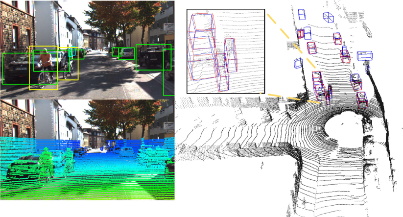
(a) KITTI dataset

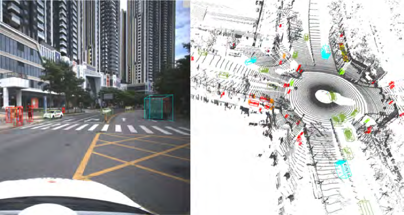
(b) SUSCAPE dataset

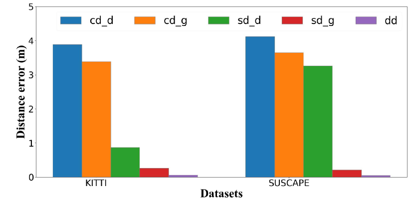
(c) Distance errors in two datasets

Figure 10: Comparison of distance errors on KITTI and SUSCAPE datasets. (a) Object detection results by Pointpillars on KITTI. Blue and red boxes denote the detected result and the ground truth, respectively. (b) Perfect object detection results on SUSCAPE, where all boxes are labeled by human experts. (c) Average distance errors of cd, sd, and dd on KITTI and SUSCAPE.

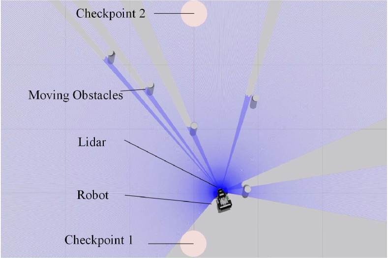
(a) 5 moving obstacles

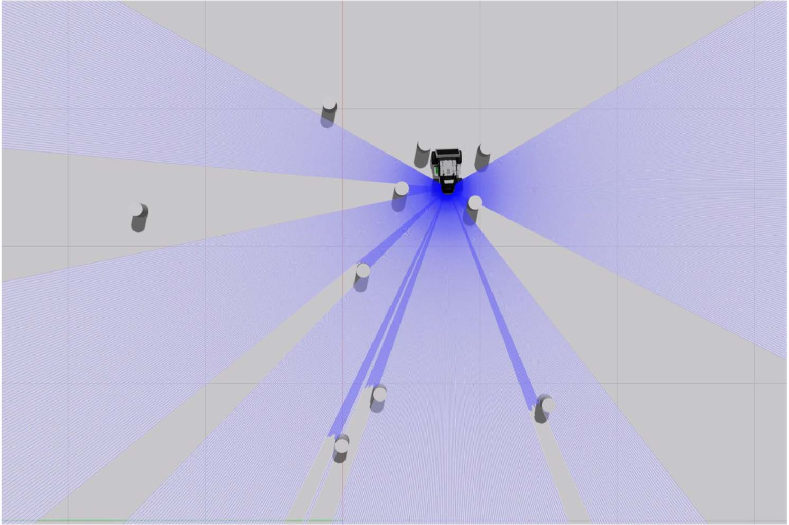
(b) 10 moving obstacles

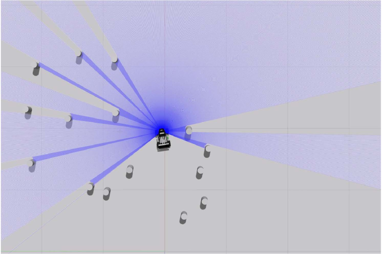
(c) 15 moving obstacles

(d) 20 moving obstacles

Figure 11: Dynamic environment navigation with different number of moving obstacles in Gazebo simulation.

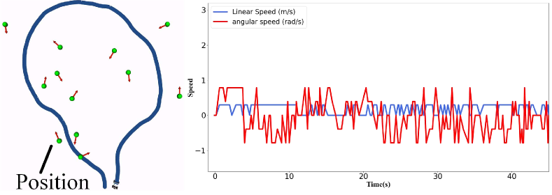
(a) AEMCARL (prone to take a detour)

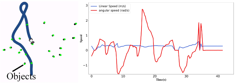
(b) RDA (prone to collision due to high computation cost)

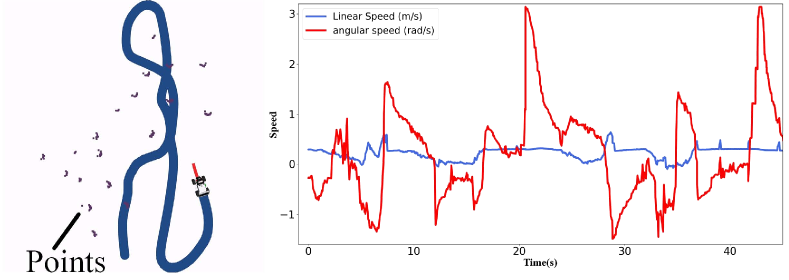
(c) NeuPAN (successful patrol)

Figure 12: Trajectory and speed comparison of different methods in Gazebo simulation.

VIII-A Experiment 1: Validation of DUNE on Open Datasets

In this subsection, real-world experiments are presented to verify the efficacy of our proposed DUNE as well as its advantage over existing methods adopting inexact distances as mentioned in Section IV-C. We consider two open-source datasets: 1) KITTI [49], which is a popular real-world urban driving dataset (see Fig. 10(a)); 2) SUSCAPE , which is a large-scale multi-modal dataset with more than $1000$ scenarios. This SUSCAPE dataset is collected and processed by ourselves based on the autonomous vehicle platform in Fig. 9(c). We calculate the minimum distance between the ego-vehicle and all surrounding objects based on three different rules: center point distance (cd), full shape set distance (sd), and our DUNE distance (dd). The computations of cd and sd based on the boxes of the object detectors are denoted by cd_d and sd_d. Here we choose a celebrated point based detector Pointpillars [50], whose accuracy achieves $74.31$% (moderate) for car detection task. The distance error is defined by the difference between the calculated distance and the ground truth distance (computed based on the raw point cloud provided by the dataset). It can be seen from Fig. 10(a) and 10(c) that the distance error of DUNE (i.e., dd error marked in purple) is significantly smaller than the errors of the other approaches, which concisely quantify the benefit brought by direct point robot navigation. As such, we can effectively overcome the detection inaccuracies inherent in conventional object detection algorithms.

Similarly, the qualitative result in the SUSCAPE dataset is shown in Fig. 10(b) and the quantitative result is shown at the right-hand side of Fig. 10(c). The results show that our DUNE distance still has the smallest error. In addition, the cd_d and sd_d errors increase compared with the result in KITTI. This is due to the lack of the generalizability of the learning based object detector. In contrast, our DUNE can be directly applied across different scenarios. Finally, one may wonder whether we can reduce this distance error by replacing Pointpillars with other highly accurate object detectors. To this end, we conduct another experiment of considering a perfect object detector with $100\,\%$ accuracy, i.e., we directly use the ground truth bounding boxes labeled by human experts as its outputs. The computations based on this detector can be denoted by cd_g and sd_g. It can be seen from Fig. 10(c) that the errors of cd_g, sd_g are smaller than that of cd_d and sd_d due to the improvement in object detection. However, these errors are still much larger than the dd error. This is because there exist a gap between the shapes of a box and a nonconvex object (e.g., pedestrian).

VIII-B Experiment 2: Agile Robot Navigation

TABLE II: Quantitative Results for Fig. 11.

Moving Obstacles	Success Rate				Navigation Time				Average Speed
	NeuPAN	RDA	AEMCARL		NeuPAN	RDA	AEMCARL		NeuPAN	RDA	AEMCARL
5	1.0	0.90	0.93		31.10	35.12	48.31		0.291	0.295	0.270
7	0.95	0.89	0.91		32.40	38.35	50.44		0.288	0.281	0.266
10	0.93	0.85	0.89		35.61	39.44	53.45		0.285	0.279	0.259
12	0.93	0.83	0.86		36.61	41.88	52.45		0.284	0.281	0.264
15	0.90	0.74	0.82		36.71	43.67	57.71		0.279	0.251	0.257
17	0.88	0.70	0.76		37.91	46.12	59.08		0.271	0.253	0.240
20	0.88	0.68	0.73		38.17	47.16	61.21		0.264	0.234	0.221

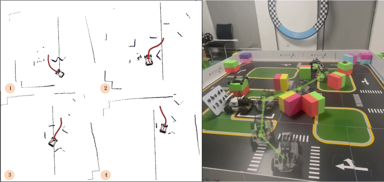
(a) Differential robot navigation through crowded cubes.

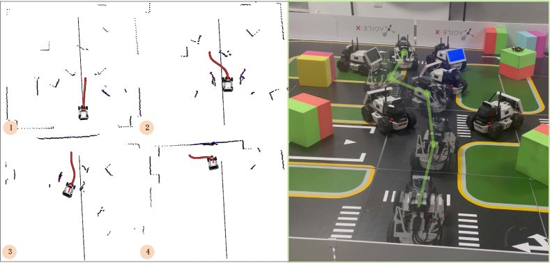
(b) Differential robot navigation through nonconvex robots.

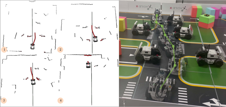
(c) Ackermann robot navigation through nonconvex robots.

Figure 13: Navigating differential and Ackermann robots in real world testbed. Red lines are NeuPAN generated trajectories. Black lines are the straight line from the start to end points. Black points are LiDAR scans.

Figure 14: Robot navigation in an unstructured cluttered environment. Green straight line is the reference path. Purple points are the raw 2D LiDAR data. Red line is the optimal receding path. Red points are the input obstacle points. 3D LiDAR is used for localization. The narrowest space (e.g. (5)) has only about 3-centimeter tolerance with degree of narrowness being $\mathsf{DoN}=0.88$.

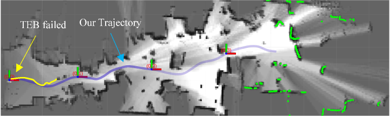
(a) Trajectories of TEB and NeuPAN in the Cartographer built grip map.

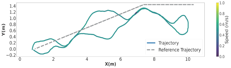
(b) Trajectory with linear speed change.

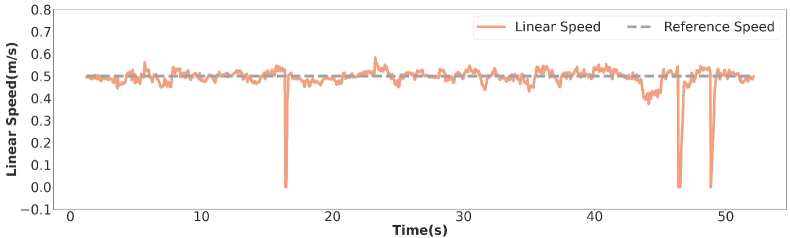
(c) Linear speed

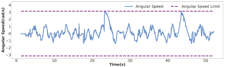
(d) Angular speed

Figure 15: Trajectory, linear, and angular speed profiles of the agile mobile robot during the office navigation task.

VIII-B1 Dynamic Environment

Navigating robots through dynamic cluttered environments using only onboard sensing and computing resources is difficult due to the stringent accuracy and latency tolerance. But here we will show that NeuPAN is qualified for the above job. In particular, we adopt Gazebo [51], a widely recognized open-source 3D robotics simulator, to demonstrate the dynamic collision avoidance capability of our approach. The experimental setup is illustrated in Fig. 11, where the robot, operating in differential steering mode, must patrol between two checkpoints as fast as possible while preventing itself from being surrounded by massive adversarial moving obstacles. The obstacles with cylinder shape are randomly placed within a region of interest and exhibit reciprocal collision avoidance behavior with speed adjustments. The robot is equipped with a LiDAR sensor to detect obstacles. We compare our method with AEMCARL [25], which is a state-of-the-art reinforcement learning based solution for dynamic collision avoidance. We choose AEMCARL as a benchmark because it has already been shown in [25] to outperform SARL [8] and RGL [31]. All these methods map ego-position and object poses into actions, which is computationally efficient but does not guarantee safety. We also compare our method with RDA [21], which is a state-of-the-art optimization based solution for dynamic collision avoidance. RDA is a full shape MPC scheme, and has already been shown in [21] to enjoy a higher frequency than the OBCA method [3]. Note that both AEMCARL and RDA require the pose and geometry information of obstacles, which are obtained from Gazebo. All these methods adopt a reference speed of $0.3\,\mathrm{m/s}$.

The evaluation consists of three metrics: success rate, navigation time, and average speed. A successful case is defined as the robot finishing a shuttle between two checkpoints without experiencing any stalling/collisions. Success rate is calculated as the proportion of successful cases out of $100$ trials. Navigation time is measured as the duration taken by the robot to complete a single shuttle. This is recorded by Gazebo simulation. Navigation with a higher speed is deemed to be more efficient. Therefore, we also compare the average speed of different schemes. Experimental results based on 100 trials with the number of obstacles ranging from 5 to 20 are presented in Table II. It can be seen that NeuPAN outperforms AEMCARL and RDA in terms of success rate, navigation time, and average speed. This corroborates the discussions in Section II.

Comparison of trajectories and speed profiles is shown in Fig. 12. First, AEMCARL is prone to take a detour in front of crowded obstacles, resulting in longer navigation time, as shown in Fig. 12(a). The main reason is that AEMCARL relies on reward functions and is more conservative compared to NeuPAN. In addition, the discrete action space also limits its flexibility. Second, RDA involves longer computation time than NeuPAN and AEMCARL, thus prone to cause collisions, resulting in lower success rate, as shown in Fig. 12(b). Lastly, NeuPAN computes exact distance from raw points and maps distances to actions with low latency, thus achieving successful patrols, as shown in Fig. 12(c).

The results of AEMCARL and NeuPAN could be even worse in real-world settings with non-ideal LiDARs. Lastly, AEMCARL (and almost all learning-based methods) requires a huge volume of training data and long-time training (in the order of days to weeks) to reach an acceptable performance. Our method, however, requires only hour-level training to obtain a stable result due to its interpretability nature, thus significantly reducing the efforts in practical deployment.

VIII-B2 Structured Real-World Testbed

Sim-to-real gap is the key bottleneck that limits the real-world applications of learning based approaches. To this end, we conduct real-world experiments in a confined testbed to demonstrate the robustness and sim-to-real generalizability of the proposed NeuPAN. The associated results are presented in Fig. 13. The robot is tasked to navigate through a crowd of obstacles to reach the goal point by onboard Livox LiDAR and Jetson Nano computer. Fig. 13(a) shows that the ego-robot under differential steering mode passes the “impassable” area filled with crowded cubes. Then, this challenge is further upgraded by replacing the box-shape cubes with nonconvex-shape robots. In such a dense and unstructured geometry, the robot driven by NeuPAN is still able to navigate efficiently, as shown in Fig. 13(b). Finally, we switch the robot mode from differential to Ackermann, which imposes more limitations on robot movements. Under the above change of robot dynamics, most existing learning-based approaches require model retraining. Nonetheless, due to the embedded physical engine in NRMP, model retraining is not needed for NeuPAN. That is, NeuPAN trained on the differential robot succeeds in directly adapting to the Ackermann robot, as demonstrated in Fig. 13(c). All these experimental results confirm the high-accurate and robot-agnostic features of NeuPAN in real-world dense (but structured) scenarios.

VIII-B3 Unstructured Real-World Environment

The above experiments have considered structured environments, where the obstacles are easy to be detected (e.g., box, wall) and classified (e.g., person, car). However, for extensive real-life applications (e.g., autonomous housekeeper ALOHA), the target scenarios are highly unstructured and disordered. To this end, we further test NeuPAN in a highly cluttered laboratory as shown in Fig. 14. The laboratory is filled with sundries, such as chair, sandbox, water bottle, equipment, etc., which are unrecognizable objects. The robot needs to patrol in this environment at a target speed of $>0.5\,$m/s without a pre-established map. First, we invite $10$ human pilots to manually control the robot. But unfortunately, all of them fail, resulting in either robot collisions or time out due to insufficient speed. Then, we adopt NeuPAN to handle this situation. This time, the task is accomplished, with the associated trajectories (marked as blue lines) illustrated in Fig. 14. The narrowest place has only about 3-centimeter tolerance with $\mathsf{DoN}=0.88$ (see Fig. 14(5)). But owing to the exact distance perception from DUNE and high accurate locomotion from NRMP, our method is able to navigate the robot through this challenging scenario with only onboard LiDAR in real time at $20\,$Hz.

The trajectories and speed profiles of NeuPAN and TEB during this task are shown in Fig. 15. We build the occupancy grid map by Cartographer [52], which is a celebrated SLAM algorithm, for TEB to plan its trajectory, as shown in Fig. 15(a). The TEB trajectory (marked in yellow) fails in the narrow space because of the limited resolution of grid map. Figs. 15(b)-15(d) illustrate the successful trajectory of NeuPAN (marked in blue) and its associated linear and angular speed profiles. It can be seen that the linear speed fluctuates around the target speed $0.5$ m/s and the angular speed is rigorously constrained within the range $[-3.14,3.14]$ rad/s, which achieves a stable and bounded control policy.

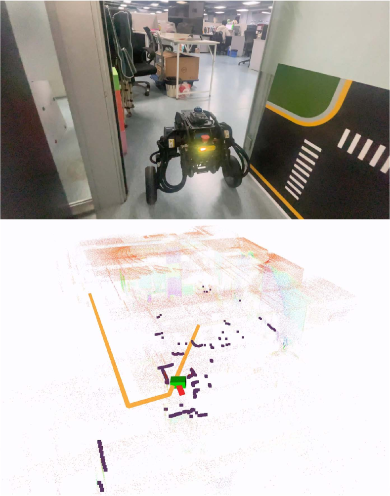
(a) Through the narrow doorway

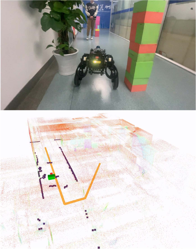
(b) Through the narrow gap

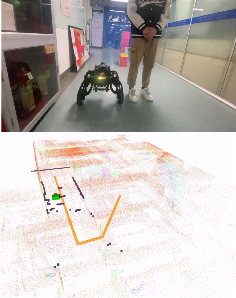
(c) Avoid human on the way

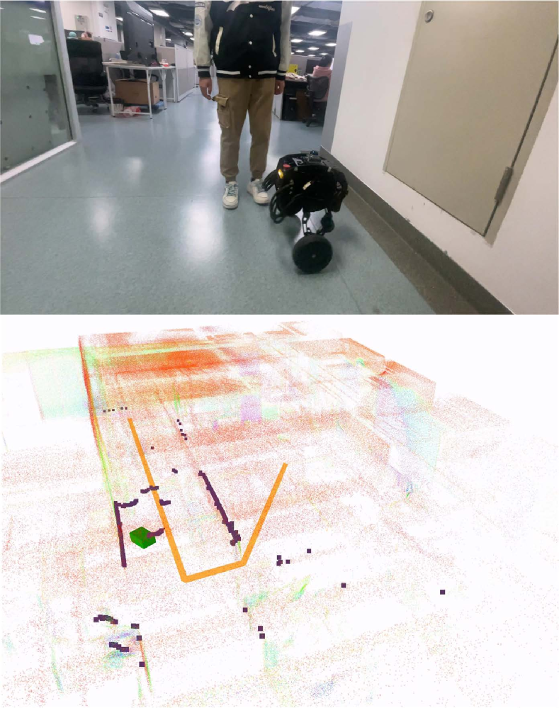
(d) Avoid the road blocker

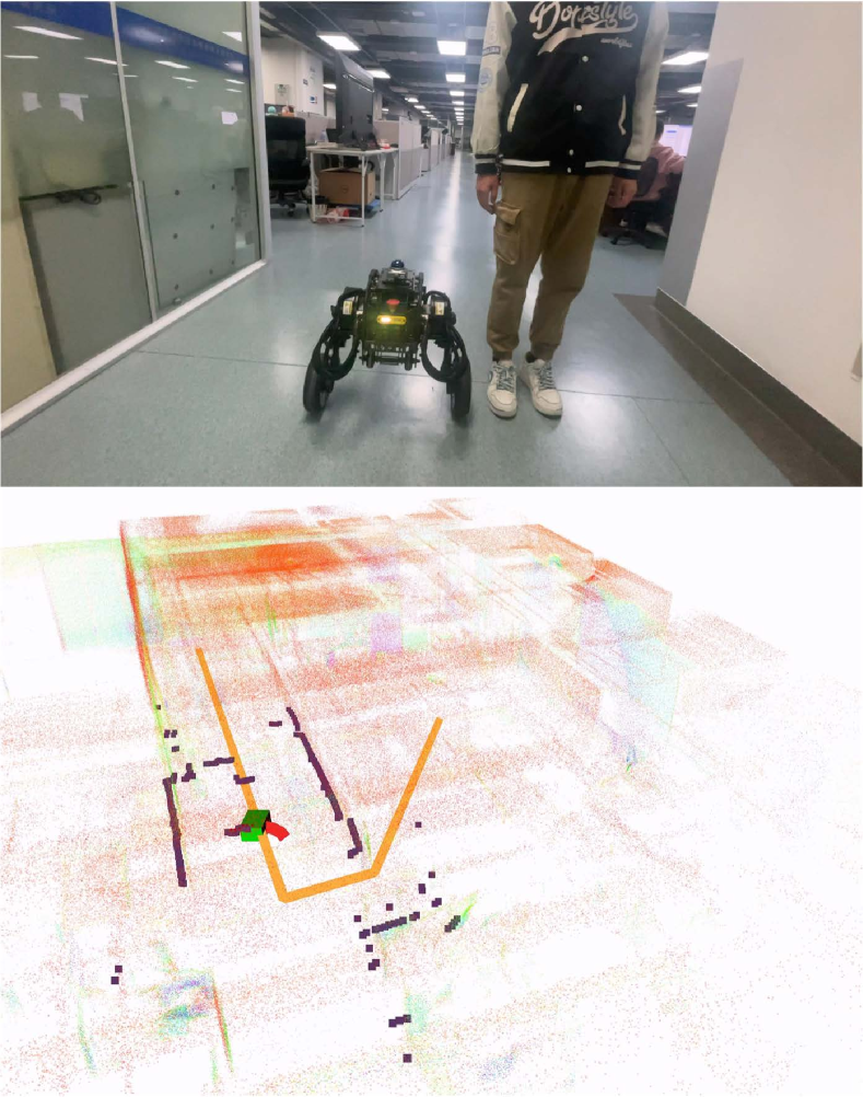
(e) Avoid the road blocker

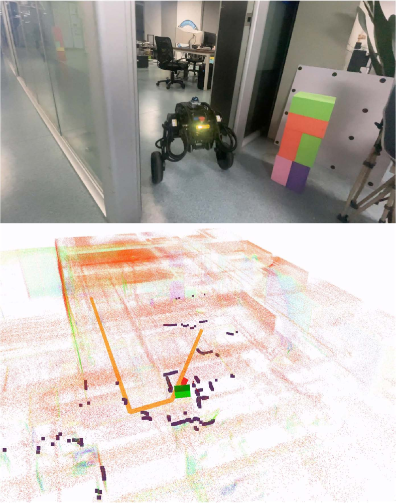
(f) Return to the start point

Figure 16: Wheel-legged robot exploration in the office.

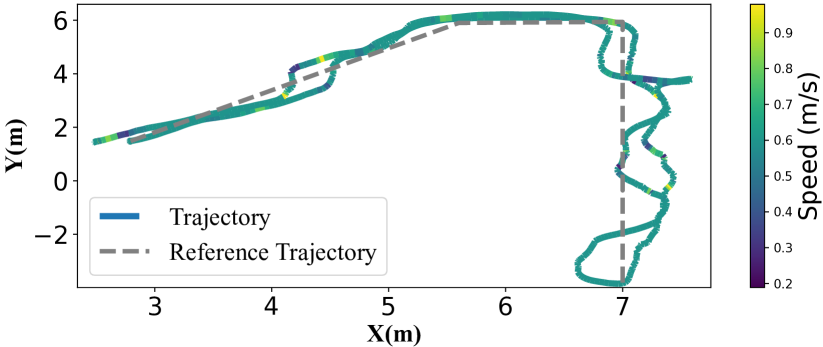
(a) Trajectory with linear speed change.

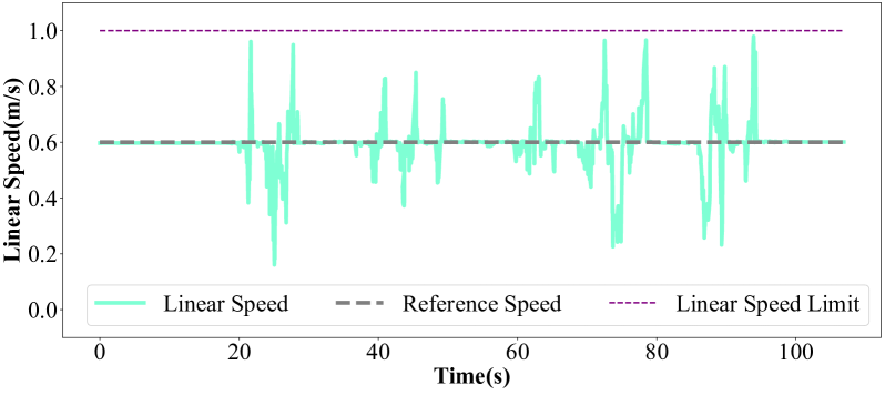
(b) Linear speed

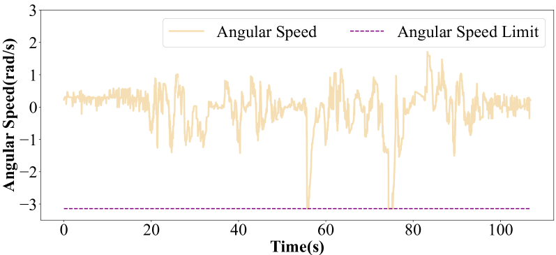
(c) Angular speed

Figure 17: Trajectory, linear, and angular speed change of the wheel-legged robot during the exploration task.

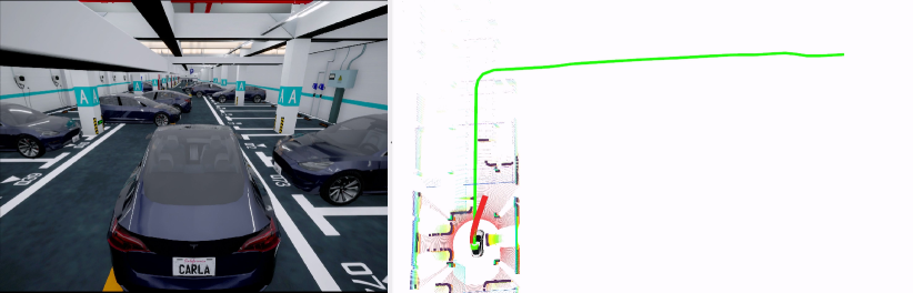
(a) Illegally parked vehicles

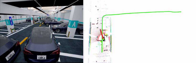
(b) Illegally parked vehicles

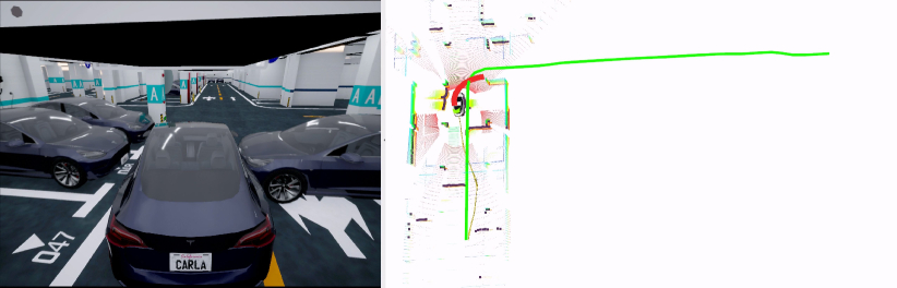
(c) Illegally parked vehicles

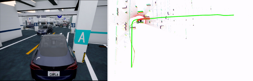
(d) Aggressive obstacle vehicle

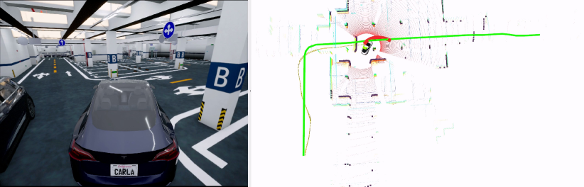
(e) Dangerous obstacle vehicle

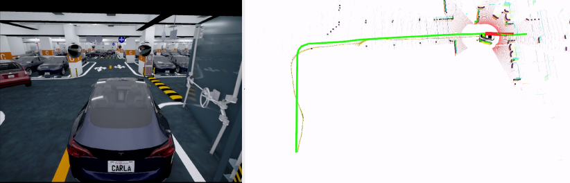
(f) traffic flow

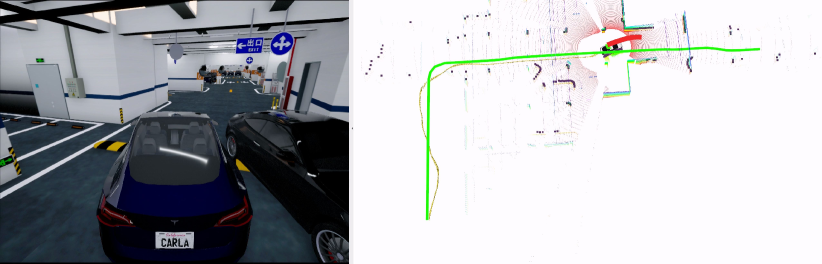
(g) Oncoming Traffic

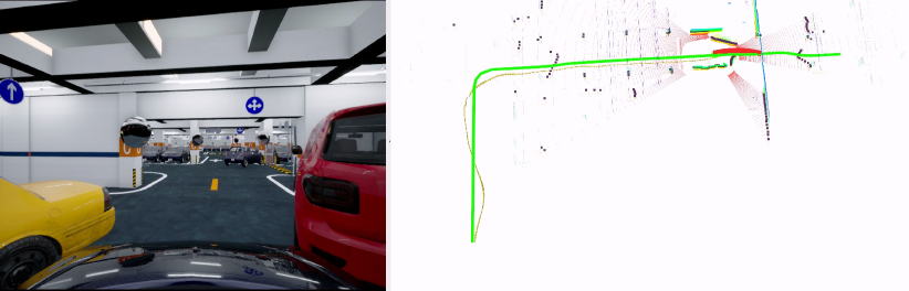
(h) Narrow Spaces

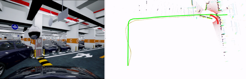
(i) Wrong Reference Path

Figure 18: Passenger vehicle navigation in Carla. (a)–(c): first phase, where the static vehicles block the road, leaving only a narrow passable space ($\mathsf{DoN}=0.97$). (d)–(f): second phase, where a traffic flow is generated randomly. (g)-(i): challenging cases during the collision avoidance of traffic flows.

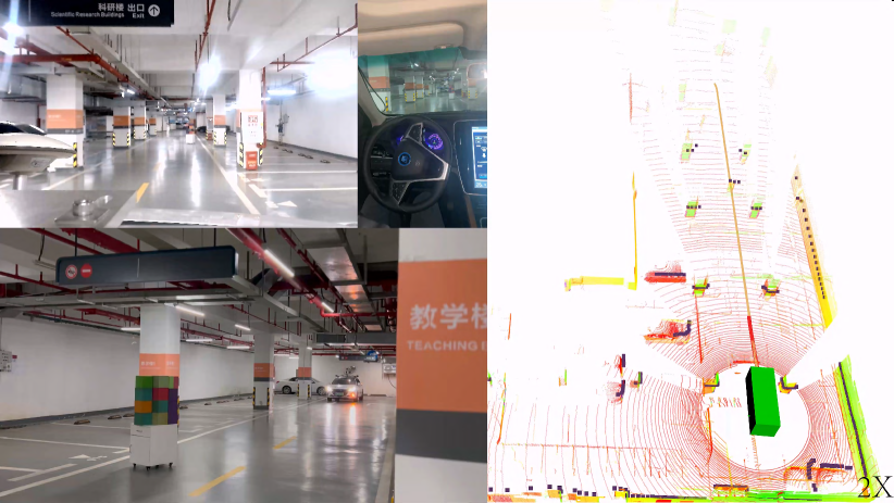
(a) Start point

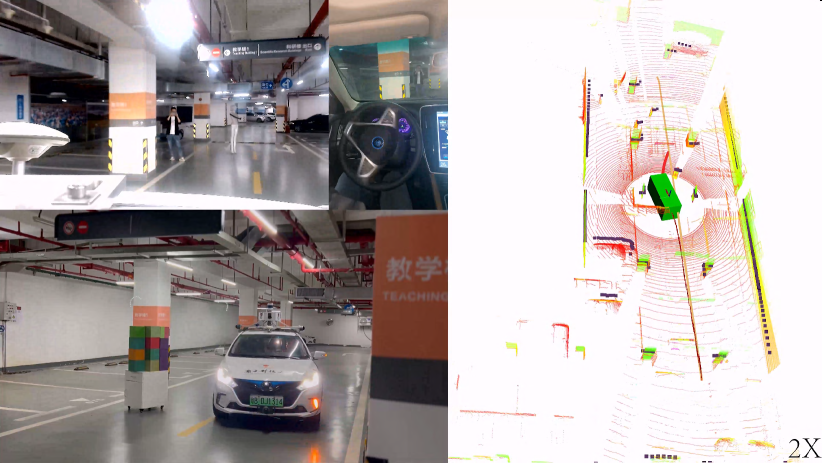
(b) Avoid the boxes

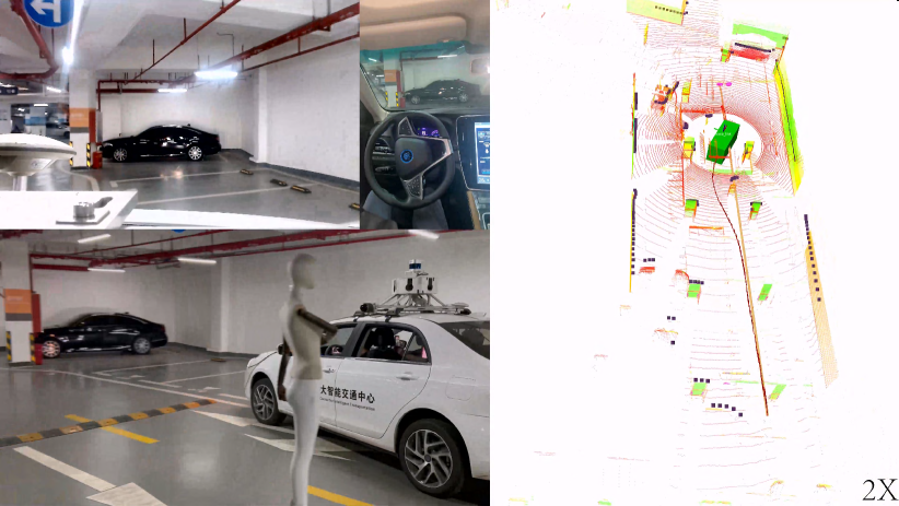
(c) Avoid the mannequins

Figure 19: Real-world experiment of passenger vehicle navigation in the parking lot with boxes, mannequins, and other vehicles.

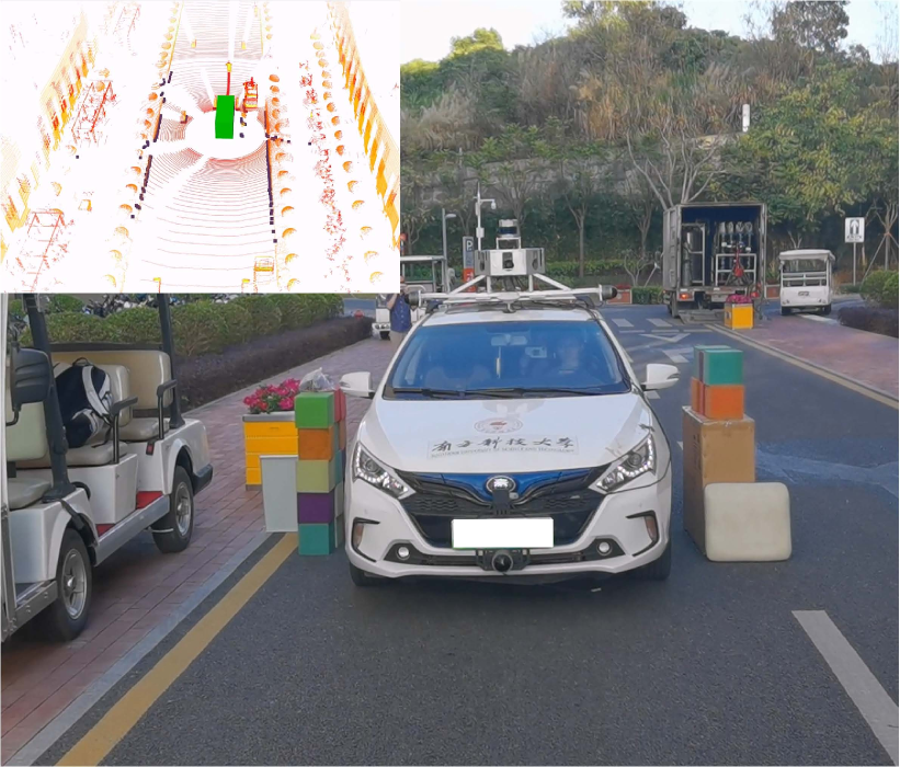
(a) Autonomous control (success)

(b) Human driving (collision)

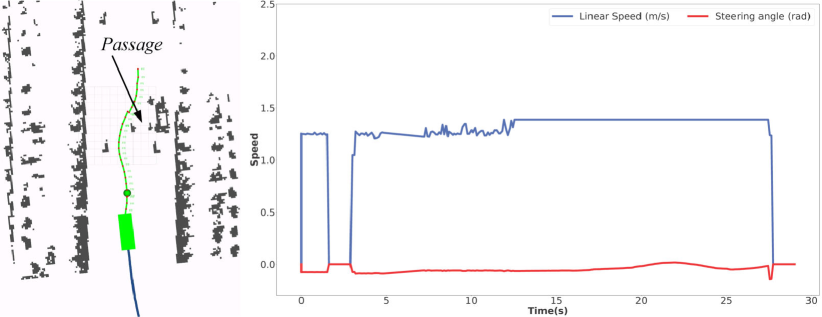
(c) Hybrid a star (Grid map).

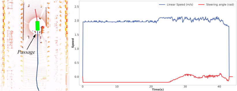
(d) NeuPAN (Point cloud).

Figure 20: Real-world experiment of passenger vehicle navigation through a narrow passage ($\mathsf{DoN}=0.97$). (a) NeuPAN succeeds at $7\,\mathrm{km/h}$. (b) Human driver fails at $5\,\mathrm{km/h}$. (c) The trajectory, linear speed and steering angle of the Hybrid A star guided passenger vehicle. (d) The trajectory, linear speed and steering angle of the NeuPAN guided passenger vehicle.

VIII-C Experiment 3: Wheel-legged Robot Navigation

In this subsection, we validate NeuPAN on a medium-size robot platform, i.e., the wheel-legged robot as mentioned in Fig. 1, to conduct autonomous exploration and dense mapping tasks in an unknown office building, as illustrated in Fig. 16. The only information given to the LiDAR-based legged robot is a reference path obtained from historical data. Fast-lio2 [47] is employed for real-time mapping of the environment and localization of the ego robot. Note that the narrowest space has a $\mathsf{DoN}$ value of $0.92$. It can be seen from Fig. 16 that there exist $3$ challenges between the starting and end points (the same position in Fig. 16(f)): 1) passing a narrow doorway (Fig. 16(a)); 2) avoiding unknown obstacles (the potted plant in Fig. 16(b)); 3) circumventing adversarial humans who suddenly rush over to block the way (Fig. 16(c)-16(e)). Due to the precise cm-level end-to-end perception-planning-control afforded by NRMP, the wheel-legged robot successfully conquered all these challenges. This experiment demonstrates the efficacy and robustness of our approach in enhancing operational capabilities of wheel-legged robots.

The quantitative results, including the trajectory, linear speed, and angular speed, are shown in Fig. 17. It is clear that the wheel-legged robot succeeds in following the waypoints and returning to the starting point. The linear speed fluctuates around the target value $0.6\,$m/s, but is rigorously controlled below $1\,$m/s (the maximum speed requested by the user). Similarly, the angular speed is rigorously controlled between $-3.14\,$rad and $+3.14\,$rad. This result show that our approach is constraints guaranteed due to the interpretability and hard-bounded constraints in NRMP, which is in contrast to learning-based solutions that may output uncertain motions.

Interpretation from biology: Note that even if its path is deliberately blocked by a human, the robot immediately gives up the original route and replans another route to continue its exploration. This response, known as a conditioned reflex in analogy to humans/animals, is also a form of learning. Such behaviors are a consequence of the learnable feature of NRMP, and allows NeuPAN no longer limited by fixed, inherited navigation patterns, but can be modified by experience and exposure to an unlimited number of environmental stimuli. This high-frequency low-level intelligence is also capable of collaborating with higher-level intelligence provided by large language/vision models. They together contribute to the most evolved nervous systems for embodied AI.

VIII-D Experiment 4: Passenger Vehicle Navigation

In this subsection, we validate NeuPAN on a large-size passenger vehicle platform. Compared to the aforementioned robots, the vehicle has a larger value of speed (e.g., $10$ to $50\,$km/h) and minimum turning radius (i.e., $6\,$m). Therefore, existing solutions for passenger vehicles adopt a safety distance of $>1\,$m, and vehicles often stop in front of confined spaces. In the following experiments, we will show that NeuPAN can overcome the above drawbacks.

VIII-D1 Simulated Environment

We employ CARLA [44], a high-fidelity simulator powered by unreal engine, to create a virtual parking lot scenario in Fig. 18. A 128-line 3D LiDAR mounted on top of the vehicle provides real-time measurements of the environment. The task is to navigate the vehicle from zone A to zone B, and consists of two phases. In the first phase, as shown in Fig. 18(a)–18(c), illegally parked vehicles block the way with $\mathsf{DoN}=0.95$. But due to the end-to-end feature, NeuPAN successfully finds the optimal way under the dynamic constraints in real time, and the successful trajectory is shown in Figs. 18(a)-18(c). In the second phase, as shown in Fig. 18(d)–18(f), an adversarial dynamic traffic flow is added to simulate the real world adversarial or even accidental traffics. For instance, in Fig. 18(e), a dangerous obstacle vehicle crash into our ego vehicle. After the crash moment, NeuPAN generates an expert-driver-like steering and accelerating action, which rehabilitates the vehicle from crash and makes a timely turn. Fig. 18(g)–18(i) illustrate other challenging cases under the dynamic traffic flows. Interestingly, Fig 18(h) presents an extreme case where the gap is too narrow for any existing method to pass. This is because the detected boxes are slightly bigger than the actual objects, making the width of remaining drivable area smaller than the width of ego vehicle. However, our methodology makes impassable passable, by maneuvering the vehicle with only $1\,$cm away from both sides of obstacles as shown in Fig 18(h). This already exceeds human-level driving, as tested by our volunteer human drivers.

VIII-D2 Real world Environment

We further apply the above network trained on the simulated data directly on the real autonomous driving vehicle to validate its sim-to-real capability. In existing works, numerous methodologies, such as end-to-end IL and RL, have demonstrated great potential in simulated environments. Nevertheless, these approaches face difficulties when applied to real-world scenarios due to the sim-to-real gap. Real-world testing can also verify the robustness of NeuPAN since hardware uncertainties (e.g., noises, impairments) are now considered.

First, we test the vehicle with a 128-line LiDAR in the parking lot as shown in Fig. 19. Real-time localization is realized using SC-Lego-Loam [53]. Unlike the wide-open environment on the road, the parking lot leaves less space for the vehicle ($\mathsf{DoN}=0.93$). Existing solutions adopt object detection or occupancy grids are prone to take a detour. In contrast, our solution successfully controls the vehicle to move with an S-shaped trajectory to avoid boxes and mannequins as illustrated in Fig. 19(a)-19(c).

Finally, we conduct a simple yet specially designed experiment to validate the performance of NeuPAN. In this challenge, the vehicle needs to pass an extremely narrow passage with width of $1.82\,$m within a certain time budget (corresponding to an average speed of $5\,$km/h). As the vehicle width is already $1.77\,$m, there is only about $5$ centimeter tolerance ($\mathsf{DoN}=0.97$). We compare the proposed approach with: 1) hybrid A star implemented by Autoware [54, 55], a state-of-the-art open-source autonomous driving solution, and 2) the human driving. First, it can be seen that even under a $\mathsf{DoN}$ close to 1, our NeuPAN solution successfully navigates the vehicle through the gap at a speed of $7km/h$, as shown in Fig. 20(a). Second, the human driver is very likely to fail given a speed of $5km/h$. Only when we reduce the speed to a lower value (e.g. $2km/h$) can the human driver tackle this situation by careful observations, as shown in Fig 20(b). Lastly, the Autoware solution, i.e., hybrid A star, converts the LiDAR scans into occupancy grids, as shown in Fig. 20(c). This approach treats the narrow gap as impassable, thereby generating alternative directions for detouring. In contrast, our NeuPAN solution directly utilizes the LiDAR points as input, achieving higher accuracy and successfully finding the optimal path, as illustrated in Fig. 20(d).

The above experiments demonstrate the advantage of the proposed framework in extremely cluttered environment. This advantage makes our approach very promising in handling difficult parking cases.

IX Conclusion

This article proposed NeuPAN, an end-to-end model-based learning approach for robot navigation. A novel tightly-coupled perception-locomotion framework, including DUNE and NRMP, is developed to directly map the raw point to the robot action with no error propagation. Owing to the interpretable deep unfolding neural network, DUNE can be trained in a sim-to-real fashion to convert lidar points to distances. The output distance features are embeded as the neural regularizers to generate collision-free robot actions by NRMP represented by the differentiable convex optimization layers. Exhaustive experiments on multiple robot platforms in diverse scenarios are conducted to validate NeuPAN, which show that NeuPAN outperforms existing state-of-the-art approaches in terms of accuracy, efficiency, robustness, and generalization capability. Since NeuPAN generates perception-aware and physically-interpretable motions in real time, it empowers autonomous systems to work in cluttered environments that are previously considered impassable, triggering new applications such as cluttered-room housekeeping and limited-space parking.

Appendix A Equivalence between P and Q

Equations with number smaller than (36) can be found in the main body of the manuscript.

To prove this, we substitute (10) and (12) into $D_{i,t}$, and substitute $D_{i,t}$ into ${\bf{dist}}(\mathbb{Z}_{t}(\mathbf{s}_{t}),\mathbb{P}_{t})$ in (8). Then, the constraint (1b) in $\mathsf{P}$ is equivalent to

$${\bf{dist}}(\mathbb{Z}_{t}(\mathbf{s}_{t}),\mathbb{P}_{t};\{{\bm{\mu}}_{t}^{i},{\bm{\lambda}}_{t}^{i}\}) \geq d_{\rm{min}}\iff$$

$$\mathop{\min_{i=1,\cdots,M}}~{}\left\{{{\bm{\lambda}}_{t}^{i}}^{\top}\left[\mathbf{t}_{t}(\mathbf{s}_{t})-\mathbf{p}_{t}^{i}\right]-{{\bm{\mu}}_{t}^{i}}^{\top}\mathbf{h}\right\} \geq d_{\rm{min}},$$ (40a)

$${\bm{\mu}_{t}^{i}}^{\top}\mathbf{G}+{\bm{\lambda}_{t}^{i}}^{\top}\mathbf{R}(\mathbf{s}_{t}) =\bm{0},$$ (40b)

$$\{\bm{\mu}_{t}^{i},{\bm{\lambda}_{t}^{i}}\}\in\mathcal{G}.$$ (40c)

Based on the definitions of $I$ in (30) and $H$ in (31), constraints (40a) and (40b) are equivalently re-written as

$$\min\left\{I(\mathbf{s}_{t},{{\bm{{\mu}}}}_{t}^{i},{\bm{\lambda}}_{t}^{i}),0\right\}=0,~{}H(\mathbf{s}_{t},{{\bm{{\mu}}}}_{t}^{i},{\bm{\lambda}}_{t}^{i})=0.$$ (41)

According to the penalty theory, the equality constraints (41) can be removed and automatically satisfied by adding penalty terms $\|\min(I,0)\|_{2}^{2}+\|H\|_{2}^{2}$ for all $(i,t)$ to the objective of $\mathsf{P}$. Then problem $\mathsf{P}$ is equivalently transformed into $\mathsf{Q}$.

Appendix B Ackermann and Differential Models

Car-like robots adhere to the ackermann model has the nonlinear kinematics function [56]:

$$f({\mathbf{s}_{t}},{\mathbf{u}_{t}})=\left[{{v_{t}}\cos({\theta_{t}})},{{v_{t}}\sin({\theta_{t}})},{\frac{{{v_{t}}\tan{\psi_{t}}}}{L}}\right]^{T},$$

where $v_{t}$ and $\psi_{t}$ are the linear speed and steering angle of the robot at time $t$, respectively. $L$ is the wheelbase. $\theta_{t}$ is the orientation of the robot. This non-linear function can be linearized into the structure of (29) by the first-order Taylor polynomial, where the associated coefficients $(\mathbf{A}_{t}$, $\mathbf{B}_{t}$, $\mathbf{c}_{t})$ at time $t$ in (29) are given by:

$$\mathbf{A}_{t} =\left[{\begin{array}[]{*{20}{c}}1&0&{-\bar{v}_{t}\sin(\bar{\theta}_{t}){\Delta t}}\\ 0&1&{\bar{v}_{t}\cos(\bar{\theta}_{t}){\Delta t}}\\ 0&0&{1}\end{array}}\right],$$ (42)

$$\mathbf{B}_{t} =\left[{\begin{array}[]{*{20}{c}}{\cos(\bar{\theta}_{t}){\Delta t}}&0\\ {\sin(\bar{\theta}_{t}){\Delta t}}&0\\ {\frac{{\tan\bar{\psi}_{t}{\Delta t}}}{L}}&{\frac{\bar{v}_{t}{\Delta t}}{{L{{\cos}^{2}}\bar{\psi}_{t}}}}\end{array}}\right],$$

$$\mathbf{c}_{t} =\left[{\begin{array}[]{*{20}{c}}{\bar{\theta}_{t}\bar{v}_{t}\sin(\bar{\theta}_{t}){\Delta t}}\\ {-\bar{\theta}_{t}\bar{v}_{t}\cos(\bar{\theta}_{t}){\Delta t}}\\ {-\frac{{\bar{\psi}_{t}\bar{v}_{t}{\Delta t}}}{{L{{\cos}^{2}}\psi_{t}}}}\end{array}}\right],$$

where $\bar{v}_{t}$ and $\bar{\psi}_{t}$ are the nominal linear speed and steering angle of the control vector $\mathbf{\bar{u}}_{t}$ at time $t$, respectively. Similarly, the differential drive robots with the control vector: linear velocity $v_{t}$ and angular velocity $\omega_{t}$ have the kinematics function $f({\mathbf{s}_{t}},{\mathbf{u}_{t}})=\left[{{v_{t}}\cos({\theta_{t}})},{{v_{t}}\sin({\theta_{t}})},{\omega_{t}}\right]^{T}$, can be modeled to be a linear form by the following coefficients:

$$\mathbf{A}_{t} =\left[{\begin{array}[]{*{20}{c}}1&0&{-\bar{v}_{t}\sin(\bar{\theta}_{t}){\Delta t}}\\ 0&1&{\bar{v}_{t}\cos(\bar{\theta}_{t}){\Delta t}}\\ 0&0&{1}\end{array}}\right],$$ (43)

$$\mathbf{B}_{t} =\left[{\begin{array}[]{*{20}{c}}{\cos(\bar{\theta}_{t}){\Delta t}}&{0}\\ {\sin(\bar{\theta}_{t}){\Delta t}}&{0}\\ {0}&{\Delta t}\\ \end{array}}\right],$$

$$\mathbf{c}_{t} =\left[{\begin{array}[]{*{20}{c}}{\bar{\theta}_{t}\bar{v}_{t}\sin(\bar{\theta}_{t}){\Delta t}}\\ {-\bar{\theta}_{t}\bar{v}_{t}\cos(\bar{\theta}_{t}){\Delta t}}\\ {0}\end{array}}\right],$$

Appendix C Proof of Theorem 1

To prove the theorem, we first define $\mathcal{X}=\{\mathcal{S},\mathcal{U}\}$ and $\mathcal{Y}=\{\mathcal{M},\mathcal{L}\}$. Let $f(\mathcal{X})=C_{0}(\mathcal{S},\mathcal{U})+\mathbb{I}_{\mathcal{F}}(\mathcal{S},\mathcal{U})$ and $g(\mathcal{Y})=\mathbb{I}_{\mathcal{G}}(\mathcal{S},\mathcal{U})$, where $\mathbb{I}_{\mathcal{F}},\mathbb{I}_{\mathcal{G}}$ are indicator functions for the feasible sets $\mathcal{F},\mathcal{G}$. Then problem $\mathcal{Q}$ is equivalently written as

$$\mathsf{M}:\min_{\begin{subarray}{c}\mathcal{X},\mathcal{Y}\end{subarray}}~{}~{} \underbrace{f(\mathcal{X})+g(\mathcal{Y})+C_{r}(\mathcal{X},\mathcal{Y})}_{:=\Psi(\mathcal{X},\mathcal{Y})}$$ (44)

It can be seen that $\Psi$ is an extended proper and lower semicontinuous function of $C_{\mathrm{e2e}}$, by incorporating constraints as indicator functions into $C_{\mathrm{e2e}}$, and $C_{r}$ is a continuous $C^{1}$ function. Based on Sections IV and V, it is clear that NeuPAN is equivalent to the following alternating discrete dynamical system in the form of $\mathcal{X}^{[k]},\mathcal{Y}^{[k]}\rightarrow\mathcal{X}^{[k]},\mathcal{Y}^{[k+1]}\rightarrow\mathcal{X}^{[k+1]},\mathcal{Y}^{[k+1]}$ (given the initial $\mathcal{X}^{[0]},\mathcal{Y}^{[0]}$):

$$\mathcal{Y}^{[k+1]} =\mathop{\mathrm{argmin}}_{\mathcal{Y}}~{}\Big{\{}{\widehat{\Psi}}(\mathcal{X}^{[k]},\mathcal{Y})\Big{\}},~{}~{}\mathsf{(DUNE)},$$ (45a)

$$\mathcal{X}^{[k+1]} =\mathop{\mathrm{argmin}}_{\mathcal{X}}~{}\Big{\{}\Psi(\mathcal{X},\mathcal{Y}^{[k+1]})$$

$$\quad\quad\quad\quad\quad+\frac{b_{k}}{2}\|\mathbf{x}-\mathbf{x}^{[k]}\|_{2}^{2}\Big{\}},~{}~{}\mathsf{(NRMP)},$$ (45b)

where $\mathbf{x}=\mathrm{vec}(\mathcal{X})$ and $\mathbf{y}=\mathrm{vec}(\mathcal{Y})$ are vectorization of sets $\mathcal{X},\mathcal{Y}$, and $\{b_{k}\}$ are positive real numbers. The function ${\widehat{\Psi}}=f+g+\widehat{C}_{r}$, where $\widehat{C}_{r}$ is an universal approximate of $C_{r}$ with the differences between their function values and gradients bounded as

$$\|\partial C_{r}(\mathcal{X},\mathcal{Y})-\partial{\widehat{C}_{r}}(\mathcal{X},\mathcal{Y})\|_{2}\leq\epsilon,$$ (46a)

$$\|C_{r}(\mathcal{X},\mathcal{Y})-{\widehat{C}_{r}}(\mathcal{X},\mathcal{Y})\|_{2}\leq\epsilon,$$ (46b)

where $\epsilon\rightarrow 0$ as the number of layers of DUNE goes to infinity.

C-A Proof of Part (i)

With the above notations and assumptions, we now prove part (i). First, substituting $\mathcal{Y}^{[k+1]}$ and $\mathcal{Y}^{[k]}$ into (45a), we have

$${\widehat{\Psi}}(\{\mathcal{X}^{[k]},\mathcal{Y}^{[k]}\}) \geq{\widehat{\Psi}}(\{\mathcal{X}^{[k]},\mathcal{Y}^{[k+1]}\}).$$ (47)

Putting $\mathcal{X}^{[k+1]}$ and $\mathcal{X}^{[k]}$ into (45b), we have

$$\Psi(\{\mathcal{X}^{[k]},\mathcal{Y}^{[k+1]}\}) \geq\Psi(\{\mathcal{X}^{[k+1]},\mathcal{Y}^{[k+1]}\})$$

$$\quad{}+\frac{b_{k}}{2}\|\mathbf{x}^{[k+1]}-\mathbf{x}^{[k]}\|_{2}^{2}\}.$$ (48)

Combining the above two equations (47)(48) leads to

$${\Psi}(\{\mathcal{X}^{[k]},\mathcal{Y}^{[k]}\})-\Psi(\{\mathcal{X}^{[k+1]},\mathcal{Y}^{[k+1]}\})\geq$$

$$\frac{b_{k}}{2}\|\mathbf{x}^{[k+1]}-\mathbf{x}^{[k]}\|_{2}^{2}-\frac{\widehat{L}_{2}+L_{2}}{2}\|\mathbf{y}^{[k+1]}-\mathbf{y}^{[k]}\|_{2}^{2},$$ (49)

where $L_{2}$ and $\widehat{L}_{2}$ are Lipschitz constants of $C_{r}$ and $\widehat{C}_{r}$, respectively. Since $C_{0}$ and $C_{r}$ are norm functions, it is clear that $L_{2}$ and $\widehat{L}_{2}$ are finite numbers. Now we consider two cases.

• $\|\mathbf{x}^{[k+1]}-\mathbf{x}^{[k]}\|_{2}\neq 0$. In this case, there always exists some $b_{k}$ such that $b_{k}>(\widehat{L}_{2}+L_{2})\frac{\|\mathbf{y}^{[k+1]}-\mathbf{y}^{[k]}\|_{2}^{2}}{\|\mathbf{x}^{[k+1]}-\mathbf{x}^{[k]}\|_{2}^{2}}$. By setting

  $$\varrho= \left[b_{k}-(\widehat{L}_{2}+L_{2})\frac{\|\mathbf{y}^{[k+1]}-\mathbf{y}^{[k]}\|_{2}^{2}}{\|\mathbf{x}^{[k+1]}-\mathbf{x}^{[k]}\|_{2}^{2}}\right]$$

  $$\times\left(1+\frac{\|\mathbf{y}^{[k+1]}-\mathbf{y}^{[k]}\|_{2}^{2}}{\|\mathbf{x}^{[k+1]}-\mathbf{x}^{[k]}\|_{2}^{2}}\right)^{-1}>0,$$ (50)

  we obtain

  $${\Psi}(\{\mathcal{X}^{[k]},\mathcal{Y}^{[k]}\})-\Psi(\{\mathcal{X}^{[k+1]},\mathcal{Y}^{[k+1]}\})\geq$$

  $$\frac{\varrho}{2}\left[\|\mathbf{x}^{[k+1]}-\mathbf{x}^{[k]}\|_{2}^{2}+\|\mathbf{y}^{[k+1]}-\mathbf{y}^{[k]}\|_{2}^{2}\right].$$ (51)

• $\|\mathbf{x}^{[k+1]}-\mathbf{x}^{[k]}\|_{2}=0$. In this case, $\|\mathbf{y}^{[k+1]}-\mathbf{y}^{[k]}\|_{2}=0$ must hold. This is because $\mathbf{y}=\mathrm{vec}(\mathcal{Y})=\mathrm{vec}(\{\mathcal{M},\mathcal{L}\})$ represents point-to-shape distance, and is uniquely defined by the robot state $\mathbf{x}$. The distances associated with two equivalent robot states are guaranteed to be the same. This is exactly why we can abandon proximal terms in DUNE. This implies that (51) also holds.

Combining the above two cases, the proof for part (i) is completed.

C-B Proof of Part (ii)

To prove part (ii), we sum up (51) from $k=0$ to $N-1$, where $N$ is a positive integer, and obtain

$$\sum_{k=0}^{N-1}\left(\|\mathbf{x}^{[k+1]}-\mathbf{x}^{[k]}\|_{2}^{2}+\|\mathbf{y}^{[k+1]}-\mathbf{y}^{[k]}\|_{2}^{2}\right)$$

$$\leq\frac{2}{\varrho}\left[{\Psi}(\mathcal{X}^{[0]},\mathcal{Y}^{[0]})-\Psi(\mathcal{X}^{[N]},\mathcal{Y}^{[N]})\right].$$ (52)

Taking $N\rightarrow\infty$, we have

$$\sum_{k=0}^{\infty}\left(\|\mathbf{x}^{[k+1]}-\mathbf{x}^{[k]}\|_{2}^{2}+\|\mathbf{y}^{[k+1]}-\mathbf{y}^{[k]}\|_{2}^{2}\right)<\infty,$$ (53)

which gives $\lim_{k\rightarrow\infty}\|\mathbf{x}^{[k+1]}-\mathbf{x}^{[k]}\|_{2}\rightarrow 0$.

C-C Proof of Part (iii)

To prove part (iii), we first take the sub-differential on both sides of (45a)(45b), which yields

$$\partial_{\mathbf{y}}{\widehat{\Psi}}(\mathbf{x}^{[k]},\mathbf{y}^{[k+1]})+c_{k}(\mathbf{y}^{[k+1]}-\mathbf{y}^{[k]})=0,$$ (54a)

$$\partial_{\mathbf{x}}{\Psi}(\mathbf{x}^{[k+1]},\mathbf{y}^{[k+1]})+b_{k}(\mathbf{x}^{[k+1]}-\mathbf{x}^{[k]})=0.$$ (54b)

Combing the above equations and $\partial\Psi=\partial f+\partial g+\partial C_{r}$, and further applying (46a), the following equation holds

$$\lim_{k\rightarrow\infty}\mathbf{dist}(0,\partial{\Psi}(\mathbf{x}^{[k]},\mathbf{y}^{[k]})=\mathbf{dist}(0,\partial{\Psi}(\mathbf{x}^{*},\mathbf{y}^{*})\leq\epsilon.$$

This proves that every limit point $\{\mathcal{X}^{*},\mathcal{Y}^{*}\}$ of $\{\mathcal{X}^{[k]},\mathcal{Y}^{[k]}\}$ is a critical point for problem $\mathsf{Q}$. Consequently, to conclude the proof, we only need to show that the sequence converges in finite steps. By leveraging the Kurdyka-Lojasiewicz (KL) property of $\Psi$ and [57][Theorem 1], it can be shown that $\{\mathcal{X}^{[k]},\mathcal{Y}^{[k]}\}$ is a Cauchy sequence and hence is a convergent sequence approaching the limit $\{\mathcal{X}^{*},\mathcal{Y}^{*}\}$.

References

- [1] Z. Fu, T. Z. Zhao, and C. Finn, “Mobile aloha: Learning bimanual mobile manipulation with low-cost whole-body teleoperation,” in arXiv, 2024.
- [2] Tesla, “AI & Robotics,” https://www.tesla.com/AI, 2023.
- [3] X. Zhang, A. Liniger, and F. Borrelli, “Optimization-based collision avoidance,” IEEE Transactions on Control Systems Technology, vol. 29, no. 3, pp. 972–983, 2020.
- [4] S. Kousik, B. Zhang, P. Zhao, and R. Vasudevan, “Safe, optimal, real-time trajectory planning with a parallel constrained bernstein algorithm,” IEEE Transactions on Robotics, vol. 37, no. 3, pp. 815–830, 2020.
- [5] C. Rösmann, F. Hoffmann, and T. Bertram, “Kinodynamic trajectory optimization and control for car-like robots,” in 2017 IEEE/RSJ International Conference on Intelligent Robots and Systems (IROS). IEEE, 2017, pp. 5681–5686.
- [6] B. Zhou, J. Pan, F. Gao, and S. Shen, “Raptor: Robust and perception-aware trajectory replanning for quadrotor fast flight,” IEEE Transactions on Robotics, vol. 37, no. 6, pp. 1992–2009, 2021.
- [7] R. Han, S. Chen, S. Wang, Z. Zhang, R. Gao, Q. Hao, and J. Pan, “Reinforcement learned distributed multi-robot navigation with reciprocal velocity obstacle shaped rewards,” IEEE Robotics and Automation Letters, vol. 7, no. 3, pp. 5896–5903, 2022.
- [8] C. Chen, Y. Liu, S. Kreiss, and A. Alahi, “Crowd-robot interaction: Crowd-aware robot navigation with attention-based deep reinforcement learning,” in 2019 International Conference on Robotics and Automation (ICRA). IEEE, 2019, pp. 6015–6022.
- [9] T. Fan, P. Long, W. Liu, and J. Pan, “Distributed multi-robot collision avoidance via deep reinforcement learning for navigation in complex scenarios,” The International Journal of Robotics Research, vol. 39, no. 7, pp. 856–892, 2020.
- [10] R. Han, S. Chen, and Q. Hao, “Cooperative multi-robot navigation in dynamic environment with deep reinforcement learning,” in 2020 IEEE International Conference on Robotics and Automation (ICRA). IEEE, 2020, pp. 448–454.
- [11] J. Tordesillas, B. T. Lopez, M. Everett, and J. P. How, “Faster: Fast and safe trajectory planner for navigation in unknown environments,” IEEE Transactions on Robotics, vol. 38, no. 2, pp. 922–938, 2021.
- [12] Z. Zhang, Y. Zhang, R. Han, L. Zhang, and J. Pan, “A generalized continuous collision detection framework of polynomial trajectory for mobile robots in cluttered environments,” IEEE Robotics and Automation Letters, vol. 7, no. 4, pp. 9810–9817, 2022.
- [13] A. Devo, G. Mezzetti, G. Costante, M. L. Fravolini, and P. Valigi, “Towards generalization in target-driven visual navigation by using deep reinforcement learning,” IEEE Transactions on Robotics, vol. 36, no. 5, pp. 1546–1561, 2020.
- [14] W. Xiao, T.-H. Wang, R. Hasani, M. Chahine, A. Amini, X. Li, and D. Rus, “Barriernet: Differentiable control barrier functions for learning of safe robot control,” IEEE Transactions on Robotics, 2023.
- [15] Y. Hu, J. Yang, L. Chen, K. Li, C. Sima, X. Zhu, S. Chai, S. Du, T. Lin, W. Wang et al., “Planning-oriented autonomous driving,” in Proceedings of the IEEE/CVF Conference on Computer Vision and Pattern Recognition, 2023, pp. 17 853–17 862.
- [16] Z. Li, W. Wang, H. Li, E. Xie, C. Sima, T. Lu, Y. Qiao, and J. Dai, “Bevformer: Learning bird’s-eye-view representation from multi-camera images via spatiotemporal transformers,” in European Conference on Computer Vision. Springer, 2022, pp. 1–18.
- [17] L. Mescheder, M. Oechsle, M. Niemeyer, S. Nowozin, and A. Geiger, “Occupancy networks: Learning 3d reconstruction in function space,” in Proceedings of the IEEE/CVF Conference on Computer Vision and Pattern Recognition, 2019, pp. 4460–4470.
- [18] A. H. Qureshi, Y. Miao, A. Simeonov, and M. C. Yip, “Motion planning networks: Bridging the gap between learning-based and classical motion planners,” IEEE Transactions on Robotics, vol. 37, no. 1, pp. 48–66, 2020.
- [19] M. Montemerlo, J. Becker, S. Bhat, H. Dahlkamp, D. Dolgov, S. Ettinger, D. Haehnel, T. Hilden, G. Hoffmann, B. Huhnke et al., “Junior: The stanford entry in the urban challenge,” Journal of field Robotics, vol. 25, no. 9, pp. 569–597, 2008.
- [20] O. Salzman and D. Halperin, “Asymptotically near-optimal rrt for fast, high-quality motion planning,” IEEE Transactions on Robotics, vol. 32, no. 3, pp. 473–483, 2016.
- [21] R. Han, S. Wang, S. Wang, Z. Zhang, Q. Zhang, Y. C. Eldar, Q. Hao, and J. Pan, “Rda: An accelerated collision free motion planner for autonomous navigation in cluttered environments,” IEEE Robotics and Automation Letters, vol. 8, no. 3, pp. 1715–1722, 2023.
- [22] W. Ding, L. Zhang, J. Chen, and S. Shen, “Epsilon: An efficient planning system for automated vehicles in highly interactive environments,” IEEE Transactions on Robotics, vol. 38, no. 2, pp. 1118–1138, 2021.
- [23] Z. Han, Y. Wu, T. Li, L. Zhang, L. Pei, L. Xu, C. Li, C. Ma, C. Xu, S. Shen et al., “An efficient spatial-temporal trajectory planner for autonomous vehicles in unstructured environments,” IEEE Transactions on Intelligent Transportation Systems, 2023.
- [24] X. Zhou, Z. Wang, H. Ye, C. Xu, and F. Gao, “Ego-planner: An esdf-free gradient-based local planner for quadrotors,” IEEE Robotics and Automation Letters, vol. 6, no. 2, pp. 478–485, 2020.
- [25] S. Wang, R. Gao, R. Han, S. Chen, C. Li, and Q. Hao, “Adaptive environment modeling based reinforcement learning for collision avoidance in complex scenes,” in 2022 IEEE/RSJ International Conference on Intelligent Robots and Systems (IROS). IEEE, 2022, pp. 9011–9018.
- [26] L. Li, Y. Miao, A. H. Qureshi, and M. C. Yip, “Mpc-mpnet: Model-predictive motion planning networks for fast, near-optimal planning under kinodynamic constraints,” IEEE Robotics and Automation Letters, vol. 6, no. 3, pp. 4496–4503, 2021.
- [27] A. Tampuu, T. Matiisen, M. Semikin, D. Fishman, and N. Muhammad, “A survey of end-to-end driving: Architectures and training methods,” IEEE Transactions on Neural Networks and Learning Systems, vol. 33, no. 4, pp. 1364–1384, 2020.
- [28] A. Francis, A. Faust, H.-T. L. Chiang, J. Hsu, J. C. Kew, M. Fiser, and T.-W. E. Lee, “Long-range indoor navigation with prm-rl,” IEEE Transactions on Robotics, vol. 36, no. 4, pp. 1115–1134, 2020.
- [29] Y. F. Chen, M. Liu, M. Everett, and J. P. How, “Decentralized non-communicating multiagent collision avoidance with deep reinforcement learning,” in 2017 IEEE International Conference on Robotics and Automation (ICRA). IEEE, 2017, pp. 285–292.
- [30] M. Everett, Y. F. Chen, and J. P. How, “Motion planning among dynamic, decision-making agents with deep reinforcement learning,” in 2018 IEEE/RSJ International Conference on Intelligent Robots and Systems (IROS). IEEE, 2018, pp. 3052–3059.
- [31] C. Chen, S. Hu, P. Nikdel, G. Mori, and M. Savva, “Relational graph learning for crowd navigation,” in 2020 IEEE/RSJ International Conference on Intelligent Robots and Systems (IROS). IEEE, 2020, pp. 10 007–10 013.
- [32] M. Bojarski, D. Del Testa, D. Dworakowski, B. Firner, B. Flepp, P. Goyal, L. D. Jackel, M. Monfort, U. Muller, J. Zhang et al., “End to end learning for self-driving cars,” arXiv preprint arXiv:1604.07316, 2016.
- [33] F. Codevilla, M. Müller, A. López, V. Koltun, and A. Dosovitskiy, “End-to-end driving via conditional imitation learning,” in 2018 IEEE International Conference on Robotics and Automation (ICRA). IEEE, 2018, pp. 4693–4700.
- [34] J. Lin, L. Wang, F. Gao, S. Shen, and F. Zhang, “Flying through a narrow gap using neural network: an end-to-end planning and control approach,” in 2019 IEEE/RSJ International Conference on Intelligent Robots and Systems (IROS). IEEE, 2019, pp. 3526–3533.
- [35] T. Salzmann, E. Kaufmann, J. Arrizabalaga, M. Pavone, D. Scaramuzza, and M. Ryll, “Real-time neural mpc: Deep learning model predictive control for quadrotors and agile robotic platforms,” IEEE Robotics and Automation Letters, vol. 8, no. 4, pp. 2397–2404, 2023.
- [36] J. Sacks and B. Boots, “Learning sampling distributions for model predictive control,” in Conference on Robot Learning. PMLR, 2023, pp. 1733–1742.
- [37] G. Williams, P. Drews, B. Goldfain, J. M. Rehg, and E. A. Theodorou, “Information-theoretic model predictive control: Theory and applications to autonomous driving,” IEEE Transactions on Robotics, vol. 34, no. 6, pp. 1603–1622, 2018.
- [38] B. Amos, I. Jimenez, J. Sacks, B. Boots, and J. Z. Kolter, “Differentiable mpc for end-to-end planning and control,” Advances in Neural Information Processing Systems, vol. 31, 2018.
- [39] A. Agrawal, S. Barratt, and S. Boyd, “Learning convex optimization models,” IEEE/CAA Journal of Automatica Sinica, vol. 8, no. 8, pp. 1355–1364, 2021.
- [40] S. P. Boyd and L. Vandenberghe, Convex optimization. Cambridge university press, 2004.
- [41] Y. Yang, M. Pesavento, Z.-Q. Luo, and B. Ottersten, “Inexact block coordinate descent algorithms for nonsmooth nonconvex optimization,” IEEE Transactions on Signal Processing, vol. 68, pp. 947–961, 2019.
- [42] K. Gregor and Y. LeCun, “Learning fast approximations of sparse coding,” in Proceedings of the 27th international conference on international conference on machine learning, 2010, pp. 399–406.
- [43] N. Shlezinger, J. Whang, Y. C. Eldar, and A. G. Dimakis, “Model-based deep learning,” Proceedings of the IEEE, 2023.
- [44] A. Dosovitskiy, G. Ros, F. Codevilla, A. Lopez, and V. Koltun, “Carla: An open urban driving simulator,” in Conference on Robot Learning. PMLR, 2017, pp. 1–16.
- [45] A. Paszke, S. Gross, F. Massa, A. Lerer, J. Bradbury, G. Chanan, T. Killeen, Z. Lin, N. Gimelshein, L. Antiga et al., “Pytorch: An imperative style, high-performance deep learning library,” Advances in Neural Information Processing Systems, vol. 32, 2019.
- [46] A. Agrawal, B. Amos, S. Barratt, S. Boyd, S. Diamond, and J. Z. Kolter, “Differentiable convex optimization layers,” Advances in Neural Information Processing systems, vol. 32, 2019.
- [47] W. Xu, Y. Cai, D. He, J. Lin, and F. Zhang, “Fast-lio2: Fast direct lidar-inertial odometry,” IEEE Transactions on Robotics, vol. 38, no. 4, pp. 2053–2073, 2022.
- [48] T. Shan and B. Englot, “Lego-loam: Lightweight and ground-optimized lidar odometry and mapping on variable terrain,” in 2018 IEEE/RSJ International Conference on Intelligent Robots and Systems (IROS). IEEE, 2018, pp. 4758–4765.
- [49] A. Geiger, P. Lenz, and R. Urtasun, “Are we ready for autonomous driving? the kitti vision benchmark suite,” in Conference on Computer Vision and Pattern Recognition (CVPR), 2012.
- [50] A. H. Lang, S. Vora, H. Caesar, L. Zhou, J. Yang, and O. Beijbom, “Pointpillars: Fast encoders for object detection from point clouds,” in Proceedings of the IEEE/CVF Conference on Computer Vision and Pattern Recognition, 2019, pp. 12 697–12 705.
- [51] N. Koenig and A. Howard, “Design and use paradigms for gazebo, an open-source multi-robot simulator,” in 2004 IEEE/RSJ International Conference on Intelligent Robots and Systems (IROS)(IEEE Cat. No. 04CH37566), vol. 3. IEEE, 2004, pp. 2149–2154.
- [52] W. Hess, D. Kohler, H. Rapp, and D. Andor, “Real-time loop closure in 2d lidar slam,” in 2016 IEEE International Conference on Robotics and Automation (ICRA). IEEE, 2016, pp. 1271–1278.
- [53] G. Kim and A. Kim, “Scan context: Egocentric spatial descriptor for place recognition within 3D point cloud map,” in Proceedings of the IEEE/RSJ International Conference on Intelligent Robots and Systems, Madrid, Oct. 2018.
- [54] K. Kurzer, “Path planning in unstructured environments: A real-time hybrid a* implementation for fast and deterministic path generation for the kth research concept vehicle,” 2016.
- [55] S. Kato, S. Tokunaga, Y. Maruyama, S. Maeda, M. Hirabayashi, Y. Kitsukawa, A. Monrroy, T. Ando, Y. Fujii, and T. Azumi, “Autoware on board: Enabling autonomous vehicles with embedded systems,” in 2018 ACM/IEEE 9th International Conference on Cyber-Physical Systems (ICCPS). IEEE, 2018, pp. 287–296.
- [56] K. M. Lynch and F. C. Park, Modern Robotics. Cambridge University Press, 2017.
- [57] J. Bolte, S. Sabach, and M. Teboulle, “Proximal alternating linearized minimization for nonconvex and nonsmooth problems,” Mathematical Programming, vol. 146, pp. 459––494, 2014.