On discrete-time arrival processes and related random motions

Abstract

We consider three kinds of discrete-time arrival processes: transient, intermediate and recurrent, characterized by a finite, possibly finite and infinite number of events, respectively. In this context, we study renewal processes which are stopped at the first event of a further independent renewal process whose inter-arrival time distribution can be defective. If this is the case, the resulting arrival process is of an intermediate nature. For non-defective absorbing times, the resulting arrival process is transient, i.e. stopped almost surely. For these processes we derive finite time and asymptotic properties. We apply these results to biased and unbiased random walks on the d-dimensional infinite lattice and as a special case on the two-dimensional triangular lattice. We study the spatial propagator of the walker and its large time asymptotics. In particular, we observe the emergence of a superdiffusive (ballistic) behavior in the case of biased walks. For geometrically distributed stopping times, the propagator converges to a stationary non-equilibrium steady state (NESS), which is universal in the sense that it is independent of the stopped process. In dimension one, for both light- and heavy-tailed step distributions, the NESS has an integral representation involving alpha-stable distributions.

MSC2020: 60G50, 60K05, 60K15, 05C81

Keywords: Defective random variables; transient renewal processes; random walks; non-equilibrium steady state; discrete-time semi Markov processes.

1 Introduction

The concept of renewal process provides a simple and powerful model to describe the occurrence in time of random sequences of events. The basic assumption is that the random time intervals between the events (also known as waiting times) are independent and identically distributed (IID). The simplest models consider waiting times that are exponentially or geometrically distributed in the continuous- and discrete-time setting, respectively. These models are in fact the classical homogeneous Poisson process and the Bernoulli process, both characterized by the Markov property. Already in the mid-twentieth century, the Markov property was relaxed by considering IID non-exponentially distributed waiting times, generating semi-Markov analogs of the above processes (see e.g. [10]). Given the vastness of the relative literature it would be futile to aim at being exhaustive. Hence, we limit ourselves to recalling some recent related papers: [6, 7, 18, 19, 24, 32, 33].

On the other hand, the very much related concept of continuous-time random walks (CTRWs), in fact a subclass of continuous-time semi-Markov processes, was introduced in the fundamental work by Montroll and Weiss [39]. Since then, it has been extensively developed in different directions. Among the many papers on the topic we refer to the following: [23, 29, 30, 31].

Remarkably, as described in the previously cited papers, models of random motions based on CTRWs proved to be able to explain anomalous diffusion phenomena, for instance, by assuming asymptotically power-law waiting times with fat-tails.

Similarly to the theory in continuous time, semi-Markov generalizations of discrete-time processes and in general semi-Markov chains have been developed as well: see for instance [2, 27, 40], or the semi-Markov generalizations of the discrete-time telegrapher’s process, see [36, 37, 12], to cite a few.

The works mentioned above consider recurrent renewal processes with IID continuous or discrete waiting times, that is they comprise infinitely many events almost surely. There are, however, classes of arrival processes (processes modeling the occurrence of events) that are transient, that is where only a finite number of events occur almost surely in an infinitely long observation time span. Such processes may sometimes arise as renewal processes which are stopped by an external event independent of the renewal process itself.

Transient arrival processes are ubiquitous in nature. Real-world examples include the annual migrations of birds or droves which are suddenly stopped or modified by the occurrence of natural catastrophes (collapse or destruction of food resources due to climate change, storms, wildfires, earthquakes, volcanic eruptions, etc.) [8]. Indeed, the occurrence of catastrophic events may force species to change regular habits (such as the recurrent annual migration for foraging) and have been identified as major driving forces that boost evolution [20]. Furthermore, transient processes are also appropriate models in other fields: in population dynamics [22], or in finance and gambling where a sequence of independent probabilistic trials, or games, are externally stopped by random or deterministic events (for instance by a stopping rule) [11, 27].

Although transient arrival processes are widespread phenomena, their appearance in the literature is relatively rare compared to their recurrent counterparts, for which a well established framework exists [16, 26, 40]. In particular, a model for transient Markov processes appears in the paper by Latouche et al. [25] in terms of a random walk model on a two-dimensional infinite graph. The authors derived expressions for the distributions of the absorbing state and time in which the arrival process is stopped. A further model on the distributions of stopping times in compound and renewal processes has been studied by Zacks et al. [50]. The authors derive explicit expressions in the case in which a standard Poisson process crosses an upper boundary, and introduce an approach for a series of similar problems for compound Poisson processes.

In this work we analyze discrete-time arrival processes which we classify as transient, recurrent or intermediate, based on having finitely many events with probability one, zero or belonging to $(0,1)$, respectively. For instance, a discrete-time renewal process with defective IID waiting times is transient. We also consider the class of recurrent discrete-time renewal processes which are stopped (or absorbed) in the state visited at the first event of a further independent renewal process of transient or recurrent type. In the former case, the resulting process is of intermediate type, whilst, in the latter, it is transient. In particular, for the cases of defective and non defective geometrically-distributed absorbing time we perform a thorough analysis by deriving the discrete probability density function of the resulting processes, their moments together with their asymptotic behavior. A similar analysis is done in the case of stopping times drawn from a discrete version of completely monotone distributions. To this end, we evoke a discrete variant of Bernstein’s theorem. As a byproduct, we show that if a Bernoulli process is stopped by a further independent, possibly defective, Bernoulli process, then the resulting dynamics is non-Markovian, and so is the associated time-changed random walk.

Indeed, we make use of such a construction to define some related biased and unbiased random walks in the $d$-dimensional infinite lattice. Properties of recurrent, transient, and intermediate arrival processes are inherited by these random walks via stochastic time-change. For them, we deduce the basic properties, such as the spatial probability density function of the position of the walker. Particular attention is given to the intermediate random walks where the stopping time follows a Bernoulli process with defective waiting times. If this walk is biased we observe the emergence of an asymptotic superdiffusive-ballistic diffusion whose fluctuations reach their maximum when the defect equals $1/2$. If, instead, the walk is unbiased the long-time asymptotics is of a diffusive nature. We further derive a stationary infinite-time propagator (the NESS) which emerges in a well-scaled continuous space limit as long as the defectivity vanishes. Recall, the concept of NESS frequently arises in the context of stochastic resetting [4, 13, 14, 46]. Here, the interpretation of the NESS is that it represents the spatial PDF of the rescaled end point of the eventually stopped sample path. This NESS is universal in the sense that it is of the same kind, irrespectively of the underlying stopped process. These results hold true for both biased and unbiased walks with light- or heavy-tailed step distributions. In particular, in dimension one, the NESS has an integral representation involving alpha-stable distributions.

The paper is organized as follows. In Section 2 we recall some basic properties of discrete-time renewal processes and of defective distributions. Further, we introduce a classification of the arrival processes investigated in this paper. Section 3 is devoted to the analysis of discrete-time renewal processes stopped at a random time instant. The stopping time is independent of the renewal process and it is possibly defective. In particular, Section 3.2.2 deals with intermediate arrival processes which emerge in case of a defective Bernoulli stopping time. Random walks governed by all the three kinds of the considered arrival processes are addressed in Section 4. We focus on general biased and unbiased random walks in $d$-dimensional lattices. We explore the classes of random walks whose features are a direct consequence of the classification we introduced in Section 2.2. In this regard, the explicit results of Section 3.2.2 allow the discussion on biased and unbiased random walks in triangular lattices. Finally, Section 4.3 is devoted to walks generated by an arbitrary recurrent renewal process with non-defective geometrically distributed stopping time and to the behavior of its NESS.

2 Preliminaries

2.1 Discrete-time renewal processes

Let us briefly recall the notion of discrete-time renewal (counting) processes ${\cal R}(t)\in\mathbb{N}_{0}=\{0,1,\dots\}$ (see e.g. [2, 35, 40]). First consider the renewal chain process

$$J_{n}=\sum_{j=1}^{n}\Delta t_{j},\qquad n\in\mathbb{N}=\{1,2,\dots\},\hskip 14.22636ptJ_{0}=0,$$ (1)

where the increments $\Delta t_{j}\in\mathbb{N}$ (‘interarrival times’ or ‘waiting times’ in the renewal picture) are IID copies of $\Delta t$ characterized by the probability density function (PDF)

$$\mathbb{P}[\Delta t=k]=\psi(k),\hskip 28.45274ptk\in\mathbb{N}.$$ (2)

Now define

$${\cal R}(t)=\max(n\geq 0:J_{n}\leq t),\hskip 28.45274pt{\cal R}(0)=0,\hskip 28.45274ptt\in\mathbb{N}_{0}.$$ (3)

The process (3), inverse to (1), counts the events up to and including time $t$. It is useful to introduce the generating function (GF) of the waiting time density:

$$\mathbb{E}u^{\Delta t}={\bar{\psi}}(u)=\sum_{t=1}^{\infty}\psi(t)u^{t},\hskip 28.45274pt|u|\leq 1.$$ (4)

Note that ${\bar{\psi}}(u)\big{|}_{u=1}=1$ reflects the normalization of the PDF (2). Recall also that ${\bar{\psi}}(u)\big{|}_{u=0}=\psi(0)=0$ due to the strict positivity of the waiting times $\Delta t$.

In the following we will denote the GF (or discrete Laplace transform if $u=e^{-s}$) of a discrete density $f(t)$ ($t\in\mathbb{N}_{0}$) by ${\bar{f}}(u)=\sum_{t=0}^{\infty}f(t)u^{t}$ with suitable $|u|$ within the radius of convergence. For discrete convolutions of two causal functions (we call a function $f(r)$ causal if $f(r)=0$ for $r<0$), say $a(t),b(t)$, supported on $t\in\mathbb{N}_{0}$ we will use the equivalence

$$(a\star b)(t)=(b\star a)(t)=:\sum_{r=0}^{t}a(r)b(t-r)=\frac{1}{t!}\frac{d^{t}}{du^{t}}[{\bar{a}}(u){\bar{b}}(u)]\big{|}_{u=0}.$$ (5)

Further, we will denote the discrete convolution powers with $(a\star)^{n}=(a\star\ldots\star a)(t)$. The discrete Heaviside unit step function defined on $r\in\mathbb{Z}$ is such that

$$\Theta(r)=\sum_{k=-\infty}^{r}\delta_{0,k}=\left\{\begin{array}[]{cl}1,&r\geq 0\\ \\ 0,&r<0\end{array}\right.\hskip 28.45274pt(r\in\mathbb{Z}).$$ (6)

Note in particular that $\Theta(0)=1$. Finally, we will use $\delta_{r,k}=\delta_{r\,k}$ as equivalent notations for the Kronecker symbol.

Let us now consider the product

$$\psi_{\cal F}(t)=\psi(t){\cal F}(t),\hskip 28.45274ptt\in\mathbb{N}$$ (7)

where ${\cal F}(t)\in[0,1]$ for every $t\in\mathbb{N}_{0}$ with at least one $t_{1}\in\mathbb{N}$ such that ${\cal F}(t_{1})>0$ and ${\cal F}(\infty)=0$. The PDF $\psi(t)$ is of the form (2). The GF of (7) then reads

$${\bar{\psi}}_{\cal F}(u)=\mathbb{E}u^{\Delta t}{\cal F}(\Delta t)=\sum_{t=1}^{\infty}{\cal F}(t)\psi(t)u^{t},$$ (8)

converging at least for $|u|\leq 1$, and contains ${\bar{\psi}}(u)$ as a special case (${\cal F}(t)=1$ for every $t\in\mathbb{N}_{0}$). Clearly we have

$${\bar{\psi}}_{\cal F}(u)\bigg{|}_{u=1}=\mathcal{Q}\in(0,1],$$ (9)

where $\psi_{\cal F}(t)={\cal F}(t)\psi(t)$ is not a proper PDF if $\mathcal{Q}<1$.

Definition 2.1.

We call random variables with PDF (7) and $\mathcal{Q}<1$ as ‘incomplete’ or ‘defective’ random variables. Accordingly, if $\mathcal{Q}=1$ we refer to ‘complete’ or ‘non-defective’ random variables.

With an abuse of terminology we will also talk of ‘defective’ and ‘non-defective’ distributions. We will consider defective distributions subsequently in more details (Section 3). A straightforward defective case is represented by ${\cal F}(t)=Q_{0}^{\,t}$, with $Q_{0}<1$ for which the GFs ${\bar{\psi}}_{\cal F}(u)={\bar{\psi}}(Q_{0}u)$ and $\left.{\bar{\psi}}_{\cal F}(u)\right|_{u=1}={\bar{\psi}}(Q_{0})=\mathcal{Q}$.

Let $R(t)$ be the counting process defined similarly to (3) but with a renewal chain $({\cal J}_{m})_{m\in\mathbb{N}_{0}}$ with IID increments having PDF (7). Consider the probability that $R(t)$ exceeds a certain value $n_{0}$ at time $t$

$$F_{n_{0}}(t)=\mathbb{P}[R(t)>n_{0}]=\mathbb{E}\Theta(t-{\cal J}_{n_{0}+1}).$$ (10)

Hence, (10) has GF

$${\bar{F}}_{n_{0}}(u)=\mathbb{E}\sum_{t={\cal J}_{n_{0}+1}}^{\infty}u^{t}=\frac{[{\bar{\psi}_{\mathcal{F}}}(u)]^{n_{0}+1}}{1-u}.$$ (11)

Note that we used the IID property so that $\mathbb{E}u^{{\cal J}_{m}}=[{\bar{\psi}_{\mathcal{F}}}(u)]^{m}$. This GF in fact contains the large-time limit of $F_{n_{0}}(t)$. Namely,

$$F_{n_{0}}(\infty)=\mathbb{P}[R(\infty)>n_{0}]=[{\bar{\psi}_{\mathcal{F}}}(u)]^{n_{0}+1}\bigg{|}_{u=1}=\mathcal{Q}^{n_{0}+1}$$ (12)

i.e. $F_{n_{0}}(\infty)=1$ if $\mathcal{F}(t)=1$ for all $t$ (non-defective). Note that the number of arrivals almost surely exceeds any finite number. On the contrary, if $\psi_{\mathcal{F}}$ is defective ($\mathcal{Q}<1$) we have $\lim_{n_{0}\to\infty}\mathbb{P}[R(\infty)>n_{0}]=0$.

In Appendices A.1 and A.2 we derive some essential features of type I variants of Sibuya and Bernoulli renewal processes, respectively which we use in some parts of our paper.

Sometimes we evoke in our paper the picture of a renewal process (RP) as a sequence of possibly dependent trials performed at integer time instants. If the outcome of a trial is a ’success’ this corresponds to an event in the renewal picture, whereas if the outcome is a ’fail’ the time instant is uneventful. For our convenience we introduce the boolean random indicator variable which is telling us the outcomes, i.e. $Z_{t}=\{0,1\}$ where $Z_{t}=1$ (success) if $t$ is eventful, and $Z_{t}=0$ (fail) if $t$ is uneventful. We fix $Z_{0}=0$ almost surely. The counting variable (3) thus writes

$${\cal R}(t)=\sum_{r=1}^{t}Z_{r},$$ (13)

indicating the number of events occurred up to and including time $t$.

2.2 Classification of arrival processes

More in general we consider simple counting processes $\mathcal{N}(t)$, i.e. integer-valued stochastic processes with non-decreasing sample paths and such that, with probability $1$, there is no time at which two or more events occur simultaneously. In analogy with [25] we refer to $\mathcal{N}(t)$ as an arrival process (AP). In the present paper we consider distinct classes of APs:

Transient arrival processes – (Type I AP):   $\mathbb{P}[{\cal N}(\infty)<\infty]=1$, corresponding to an almost surely finite number of events with waiting times that can be infinite with strictly positive probability. This class contains the discrete-time renewal processes with defective inter-arrival distribution (‘defective RP’ for simplicity), introduced above.

Recurrent arrival processes – (Type II AP):  $\mathbb{P}[{\cal N}(\infty)=\infty]=1$, corresponding to an infinite number of events with almost surely finite waiting times. This class contains discrete-time renewal processes with non-defective inter-arrival distribution.

Intermediate arrival processes (IAPs):   $\mathbb{P}[{\cal N}(\infty)<\infty]={\cal Q}$,   ${\cal Q}\in(0,1)$. IAPs are in a sense between type I and type II.

Let $P(n_{0},t)=\mathbb{P}[{\cal N}(t)>n_{0}]$ and define the limiting quantity

$$\Lambda=\lim_{n_{0}\to\infty}\lim_{t\to\infty}P(n_{0},t)=\lim_{n_{0}\to\infty}P(n_{0},\infty),$$ (14)

where with the first limit ($t\to\infty$) we record all sample paths which ever occur with more than $n_{0}$ events. The second one ($n_{0}\to\infty$) gives the probability whether among them there are sample paths exceeding a sufficiently large number $n_{0}$ of events. We identify $\Lambda=\mathbb{P}[{\cal N}(\infty)=\infty]$ with the probability that AP ${\cal N}(t)$ never stops and the complementary probability with $\mathbb{P}[{\cal N}(\infty)<\infty]=1-\Lambda$.

Remark 2.2.

Note that

• (i) Type I APs have $\Lambda=0$: ${\cal N}(t)$ stops a.s.

• (ii) $\Lambda=1$ refers to type II APs: ${\cal N}(t)$ never stops a.s.

• (iii) $\Lambda=1-{\cal Q}\in(0,1)$ characterizes IAPs: ${\cal N}(t)$ stops with probability $1-\Lambda$.

In case (i) the number of events which ever occur almost surely does not exceed a sufficiently large $n_{0}$. As a consequence, ${\cal N}(t)$ is almost surely stopped. In case (ii) we can choose $n_{0}$ as large as we want; there are still infinitely many sample paths with more than $n_{0}$ events. The interpretation is that ${\cal N}(t)$ never stops almost surely. Finally, in case (iii), there is a probability $\Lambda\in(0,1)$ that ${\cal N}(t)$ never stops.

3 Externally stopped arrival processes

3.1 Non-defective absorbing time

Consider now a non-defective RP (that is a renewal type II AP) $N_{II}(t)$ which is ’externally’ stopped at the random time instant, independent of $N_{II}(t)$, defined as $\Delta T=\inf(r\in\mathbb{N}:N_{S}(r)\geq 1)$, i.e. at the first arrival time of another type II RP, say $N_{S}(t)$, independent of $N_{II}(t)$. Recall $N_{II}(0)=N_{S}(0)=0$ and let $\Delta T$ with non-defective PDF $\mathbb{P}[\Delta T=t]=\psi_{S}(t)$. We denote by $J_{n}^{II}$ the renewal times of $N_{II}(t)$. Consider now the AP $M(t)\in\mathbb{N}_{0}$, $t\in\mathbb{N}_{0}$, such that

$$M(t)=\Theta(\Delta T-1-t)N_{II}(t)+\Theta(t-\Delta T)N_{II}(\Delta T),\hskip 28.45274ptM(0)=0,\hskip 28.45274pt\Delta T\in\mathbb{N}.$$ (15)

The main goal of this section is to explore the properties of $M(t)$.

We observe that $M(t)$ behaves as $N_{II}(t)$ for $t<\Delta T$ and it is randomly stopped at $\Delta T\in\mathbb{N}$, the ‘stopping time’ (we will also use the term ‘absorbing time’). After the stopping, the process keeps the value $M(\Delta T)=N_{II}(\Delta T)$ forever. The contribution $\Theta(\Delta T-1-t)N_{II}(t)$ can be seen as a resetting term: it behaves as $N_{II}(t)$ for $t<\Delta T$ and it is set to zero at the absorbing time instant $t=\Delta T$. For what follows, it is convenient to introduce the indicator function

$$\Theta(a,t,b) =\Theta(t-a)-\Theta(t-b)$$

$$=\sum_{r=a}^{b-1}\delta_{t,r}=\left\{\begin{array}[]{l}1,\hskip 28.45274pt{\rm for}\hskip 14.22636pta\leq t\leq b-1\\ \\ 0,\hskip 28.45274pt{\rm otherwise}\end{array}\right.(a,b,t\in\mathbb{N}_{0},\hskip 7.11317pta<b).$$ (19)

In particular, we have $\Theta(J_{n}^{II},t,J_{n+1}^{II})=1$ when $N_{II}(t)=n$ and zero otherwise (consult also [36] for some details). Then, we can represent $N_{II}(t)$ as

$$N_{II}(t)=\sum_{\ell=1}^{\infty}\Theta(t-J^{(II)}_{\ell}),$$ (20)

where the summation starts at $\ell=1$ to ensure that $N_{II}(0)=0$.

Proposition 3.1.

Let ${\cal P}_{II}(v,t)=\mathbb{E}v^{N_{II}(t)}$ be the state polynomial of $N_{II}(t)$ . Then its GF ${\bar{\cal P}}_{II}(v,u)$ is

$$\begin{array}[]{clr}\displaystyle{\bar{\cal P}}_{II}(v,u)&=\displaystyle\frac{1-{\bar{\psi}}_{II}(u)}{1-u}\frac{1}{1-v{\bar{\psi}}_{II}(u)},&\displaystyle|v|\leq 1,\hskip 14.22636pt|u|<1.\end{array}$$ (21)

Proof.

By definition of the state polynomial (consult [35, 36, 37] for details and applications)

$${\cal P}_{II}(v,t)=\sum_{n=0}^{\infty}\mathbb{P}[N_{II}(t)=n]v^{n},\hskip 28.45274pt|v|\leq 1$$ (22)

where $\mathbb{P}[N_{II}(t)=n]=\Phi_{II}^{(n)}(t)=\mathbb{E}\Theta(J_{n}^{II},t,J_{n+1}^{II})$ are the state probabilities. The series in (22) stops at $n=t$ as $N_{II}(t)\leq t$ almost surely, which makes it a polynomial of degree $t$. The state probabilities have then the GFs

$$\begin{array}[]{clr}\displaystyle{\bar{\Phi}}_{II}^{(n)}(u)&=\displaystyle\mathbb{E}\sum_{t=J_{n}^{II}}^{J_{n+1}^{II}-1}u^{t}=\mathbb{E}u^{J_{n}^{II}}\sum_{r=0}^{\Delta t_{n+1}-1}u^{r}&\\ \\ &=\displaystyle\frac{1-\mathbb{E}u^{\Delta t_{n+1}}}{1-u}\prod_{j=1}^{n}\mathbb{E}u^{\Delta t_{j}}=[{\bar{\psi}}_{II}(u)]^{n}\frac{1-{\bar{\psi}}_{II}(u)}{1-u}&\hskip 14.22636pt|u|<1,\hskip 14.22636ptn\in\mathbb{N}_{0}\end{array}$$ (23)

where $\mathbb{E}u^{\Delta t_{j}}={\bar{\psi}}_{II}(u)$ ($\forall j\in\mathbb{N}$) and we have used $J_{n+1}^{II}=J_{n}^{II}+\Delta t_{n+1}$ and that the $\Delta t_{j}$ are IID. The GF of the state polynomial (22) then is

$$\begin{array}[]{clr}\displaystyle{\bar{\cal P}}_{II}(v,u)&=\displaystyle\sum_{n=0}^{\infty}{\bar{\Phi}}_{II}^{(n)}(u)v^{n}&\\ \\ &=\displaystyle\frac{1-{\bar{\psi}}_{II}(u)}{1-u}\sum_{n=0}^{\infty}v^{n}[{\bar{\psi}}_{II}(u)]^{n}&\\ \\ &=\displaystyle\frac{1-{\bar{\psi}}_{II}(u)}{1-u}\frac{1}{1-v{\bar{\psi}}_{II}(u)},&\displaystyle|v|\leq 1,\hskip 14.22636pt|u|<1,\end{array}$$ (24)

which converges absolutely as ${\bar{\psi}}_{II}(u)<1$ for $|u|<1$. ∎

Proposition 3.2.

The GF of the expected number of arrivals $\mathbb{E}N_{II}(t)$ writes

$$\begin{array}[]{ll}\displaystyle\overline{\mathbb{E}N_{II}}(u)&=\displaystyle\frac{{\bar{\psi}}_{II}(u)}{(1-u)(1-{\bar{\psi}}_{II}(u))},\qquad|u|<1.\end{array}$$ (25)

Proof.

The GF of the expected number of arrivals $\mathbb{E}N_{II}(t)$ can be written as (see (20))

$$\begin{array}[]{ll}\displaystyle\overline{\mathbb{E}N_{II}}(u)&=\displaystyle\sum_{t=0}^{\infty}u^{t}\mathbb{E}{N}_{II}(t),\qquad|u|<1\\ \\ &=\displaystyle\mathbb{E}\sum_{\ell=1}^{\infty}\sum_{t=J^{(II)}_{\ell}}^{\infty}u^{t}=\displaystyle\mathbb{E}\sum_{\ell=1}^{\infty}u^{\Delta t_{1}+\dots+\Delta t_{\ell}}\sum_{t^{\prime}=0}^{\infty}u^{t^{\prime}}\\ \\ &=\displaystyle\frac{1}{1-u}\sum_{\ell=1}^{\infty}[{\bar{\psi}}_{II}(u)]^{\ell}=\displaystyle\frac{{\bar{\psi}}_{II}(u)}{(1-u)(1-{\bar{\psi}}_{II}(u))}=\frac{\partial}{\partial v}{\bar{\cal P}}_{II}(v,u)\bigg{|}_{v=1}.\end{array}$$ (26)

∎

Further of interest for later use is the GF of the second moment.

Proposition 3.3.

We have

$$\begin{array}[]{clr}\displaystyle\overline{\mathbb{E}N^{2}_{II}}(u)&=\displaystyle\frac{{\bar{\psi}}_{II}(u)[1+{\bar{\psi}}_{II}(u)]}{(1-u)[1-{\bar{\psi}}_{II}(u)]^{2}},\qquad|u|<1.&\end{array}$$ (27)

Proof.

$$\begin{array}[]{clr}\displaystyle\overline{\mathbb{E}N^{2}_{II}}(u)&=\displaystyle\sum_{t=0}^{\infty}u^{t}\mathbb{E}N_{II}^{2}(t)=\sum_{n=0}^{\infty}{\bar{\Phi}}_{II}^{(n)}(u)n^{2}=\sum_{n=0}^{\infty}{\bar{\Phi}}_{II}^{(n)}(u)n(n-1)+\sum_{n=0}^{\infty}{\bar{\Phi}}_{II}^{(n)}(u)n&\\ \\ &=\displaystyle\left[\frac{\partial^{2}}{\partial v^{2}}+\frac{\partial}{\partial v}\right]{\bar{\cal P}}_{II}(v,u)\bigg{|}_{v=1}=\frac{{\bar{\psi}}_{II}(u)[1+{\bar{\psi}}_{II}(u)]}{(1-u)[1-{\bar{\psi}}_{II}(u)]^{2}}.&\end{array}$$ (28)

∎

The following representation of (15)

$$M(t)=\Theta(\Delta T-1-t)\sum_{\ell=1}^{\infty}\Theta(t-J^{(II)}_{\ell})+\Theta(t-\Delta T)\sum_{\ell=1}^{\infty}\Theta(\Delta T-J^{(II)}_{\ell})$$ (29)

will be useful in the next theorem that gives the state probabilities of $M(t)$.

Theorem 3.4.

Let $M(t)$ be defined as in (15), and $N_{S}(t),N_{II}(t)$ be independent RPs of type II. The PDF of $M(t)$ reads

$$P_{m}(t) := \mathbb{P}[M(t)=m]=\Phi_{S}^{(0)}(t)\Phi_{II}^{(m)}(t)+\sum_{r=1}^{t}\psi_{S}(r)\Phi_{II}^{(m)}(r)$$ (30)

$$= \sum_{r=1}^{\infty}\psi_{S}(r)\left(\Phi_{II}^{(m)}(t)\Theta(r-t-1)+\Phi_{II}^{(m)}(r)\Theta(t-r)\right)$$

where $m\in\mathbb{N}_{0}$, $\Phi_{II}^{(m)}(r)=\mathbb{P}[N_{II}(r)=m]$ and $\Phi_{S}^{(0)}(t)=\mathbb{P}[N_{S}(t)=0]$.

Proof.

First consider that

$$P_{n}(t)=\mathbb{P}[M(t)=n,N_{S}(t)=0]+\mathbb{P}[M(t)=n,N_{S}(t)\geq 1],$$ (31)

with $n,t\in\mathbb{N}_{0}$ and initial condition $P_{n}(t)\big{|}_{t=0}=\delta_{n,0}$. In this relation the event $\{M(t)=n\}$ may occur either if $N_{II}(t)=n$ and is not stopped yet (first term), or when it is stopped and $N_{II}(\Delta T)=n$ (second term). Hence, the first term writes

$$\mathbb{P}[N_{II}(t)=n,N_{S}(t)=0]=\mathbb{E}\mathbf{1}_{\{N_{II}(t)=n\}}\mathbf{1}_{\{N_{S}(t)=0\}}=\mathbb{E}\Theta(J_{n}^{II},t,J_{n+1}^{II})\mathbb{E}\Theta(\Delta T-1-t)$$ (32)

by the independence of $N_{II}(t)$ and $N_{S}(t)$. Here the probability

$$\mathbb{P}[N_{II}(t)=n]=\mathbb{E}\Theta(J_{n}^{II},t,J_{n+1}^{II})=\mathbb{P}[M(t)=n|t\leq\Delta T-1]$$ (33)

is in fact the conditional probability that $\{M(t)=n\}$ given $\{t\leq\Delta T-1\}$. Further,

$$\mathbb{E}\Theta(\Delta T-1-t)=\mathbb{P}[N_{S}(t)=0]=\Phi_{S}^{(0)}(t)=\mathbb{P}[t<\Delta T]=1-\sum_{r=1}^{t}\psi_{S}(r)$$ (34)

is the (survival) probability $\Delta T-1$ evaluated at $t$.
The second term in (31) is the joint probability that the process is absorbed and counts $n$ events, namely

$$\begin{array}[]{clr}\displaystyle H_{n}(t):=\displaystyle\mathbb{P}[M(t)=n,N_{S}(t)\geq 1]&=\mathbb{E}\Theta(J_{n}^{II},\Delta T,J_{n+1}^{II})\Theta(t-\Delta T)\\ \\ &=\displaystyle\sum_{r=1}^{t}\mathbb{P}[\Delta T=r]\mathbb{P}[N_{II}(r)=n]=\displaystyle\sum_{r=1}^{t}\psi_{S}(r)\Phi_{II}^{(n)}(r)&\end{array}$$ (35)

where we interpret $\Phi_{II}^{(n)}(r)=\mathbb{P}[M(t)=n|\Delta T=r]$, $t\geq r$, as the conditional probability that $M(t)$ counts $n$ events given that $\Delta T=r$. All the terms together complete the proof. ∎

Corollary 3.5.

Consider now the state probabilities (30), then we have the following normalization condition

$$\sum_{m=0}^{\infty}P_{m}(t)=\sum_{r=1}^{\infty}\psi_{S}(r)=1.$$ (36)

Proof.

The result follows necessarily observing that $\Phi_{II}^{(m)}(t)\Theta(r-t-1)+\Phi_{II}^{(m)}(r)\Theta(t-r)<1$. ∎

We observe that $P_{m}(t)=0$ for $m>t$ inheriting this feature from $N_{II}(t)$ and the initial condition $P_{m}(t)\big{|}_{t=0}=\Phi_{II}^{(m)}(t))\big{|}_{t=0}=\delta_{m,0}$. Then we can define the GF (state polynomial of $M(t)$ which is of degree $t$)

$$\begin{array}[]{clr}\displaystyle{\cal P}_{M}(v,t)&=:\displaystyle\mathbb{E}v^{M(t)}=\sum_{m=0}^{t}P_{m}(t)v^{m}&\\ \\ &=\displaystyle\sum_{r=1}^{\infty}\psi_{S}(r)\left\{{\cal P}_{II}(v,t)\Theta(r-t-1)+{\cal P}_{II}(v,r)\Theta(t-r)\right\}.&\end{array}$$ (37)

From the state polynomial we obtain all the moments of $M(t)$. In particular, recalling Proposition 3.2, the expected number of arrivals at time $t$ is

$$\begin{array}[]{clr}\displaystyle\mathbb{E}M(t)&=\displaystyle\mathbb{E}\Theta(\Delta T-1-t)\mathbb{E}N_{II}(t)+\mathbb{E}\Theta(t-\Delta T)N_{II}(\Delta T)&\\ \\ &=\displaystyle\frac{\partial}{\partial v}\mathbb{E}v^{M(t)}\bigg{|}_{v=1}=\sum_{r=1}^{\infty}\psi_{S}(r)\left\{\Theta(r-t-1)\mathbb{E}N_{II}(t)+\Theta(t-r)\mathbb{E}N_{II}(r)\right\}.&\end{array}$$ (38)

Analogously, from Proposition 3.3, we deduce the second moment as

$$\mathbb{E}M^{2}(t)=\left(\frac{\partial^{2}}{\partial v^{2}}+\frac{\partial}{\partial v}\right)\mathbb{E}v^{M(t)}\bigg{|}_{v=1}=\sum_{r=1}^{\infty}\psi_{S}(r)\left\{\Theta(r-t-1)\mathbb{E}N_{II}^{2}(t)+\Theta(t-r)\mathbb{E}N_{II}^{2}(r)\right\}.$$ (39)

For the moments of order $\ell\in\mathbb{N}$ we can write

$$\mathbb{E}M^{\ell}(t)=\mathbb{E}\Theta(\Delta T-1-t)\mathbb{E}N_{II}^{\ell}(t)+\mathbb{E}\Theta(t-\Delta T)N_{II}^{\ell}(\Delta T)$$ (40)

as a consequence of representation (15) and by using the properties of the indicator functions. We point out that the results of this section, in particular Theorem 3.4, hold if $N_{S}(t)$ is of type II. It is interesting to extend the result to the case in which $N_{S}(t)$ is of type I. We devote Section 3.2 to this issue and classify the types of $M(t)$. Especially, we prove there that $M(t)$ is a type I arrival process if $N_{S}(t)$ is of type II.

3.1.1 Asymptotic behavior

It is useful to consider now the GF of the probability $H_{n}(t)$ defined in (35) which writes

$$\begin{array}[]{l}\displaystyle{\bar{H}}_{n}(u)=\sum_{r=1}^{\infty}\psi_{S}(r)\Phi_{II}^{(n)}(r)\sum_{t=r}^{\infty}u^{t}=\displaystyle\frac{1}{1-u}\sum_{r=1}^{\infty}\psi_{S}(r)\Phi_{II}^{(n)}(r)u^{r}.\end{array}$$ (41)

This relation involves $\chi_{n}(t)=\psi_{S}(t)\Phi_{II}^{(n)}(t)$ which is a defective PDF with respect to $t$ and also with respect to $n$, see (9). The large time limit $H_{n}(\infty)$ gives the probability to observe a given number $n$ of events in the almost surely absorbed process. From this we can get the large time limit of the expected number of arrivals in the almost surely absorbed process as

$$\mathbb{E}\,M(\infty)\,=\sum_{m=0}^{\infty}mH_{m}(\infty).$$ (42)

A sufficient condition for the finiteness of (42) is given in the following proposition.

Proposition 3.6.

Let $\mathbb{E}\Delta T<\infty$. Then

$$\mathbb{E}M(t)\leq C^{\prime}t^{-\nu-1}t+\sum_{r=1}^{t}r\psi_{S}(r),$$ (43)

and $\mathbb{E}M(\infty)<\infty$.

Proof.

From (38),

$$\mathbb{E}M(t)=\Phi_{S}^{(0)}(t)\mathbb{E}N_{II}(t)+\sum_{r=1}^{t}\psi_{S}(r)\mathbb{E}N_{II}(r).$$ (44)

By hypothesis, $\Delta T$ has a finite mean. Hence, the PDF $\psi_{S}(t)$ tends to zero at least as $\psi_{S}(t)\sim Ct^{-2-\nu}$, $\nu\in(0,1)$, and the survival probability at least as $\Phi_{S}^{(0)}(t)\sim C^{\prime}t^{-1-\nu}$ where $C,C^{\prime}>0$ are constants. Thus we have, for large values of $t$,

$$\mathbb{E}M(t)\leq C^{\prime}t^{-\nu-1}t+\sum_{r=1}^{t}r\psi_{S}(r),$$ (45)

where we have used that $\mathbb{E}N_{II}(r)\leq t$, for every $r\leq t$. Hence,

$$C^{\prime}t^{-\nu-1}t+\sum_{r=1}^{t}r\psi_{S}(r)\sim C^{\prime}t^{-\nu}+\mathbb{E}\Delta T.$$ (46)

Moreover,

$$\mathbb{E}M(\infty)=\mathbb{E}N_{II}(\Delta T)=\sum_{r=1}^{\infty}\psi_{S}(r)\mathbb{E}N_{II}(r)<\infty.$$ (47)

∎

Remark 3.7.

For $\mathbb{E}\Delta T$ to be finite, $N_{S}(t)$ needs to be of type II with the resetting term decaying at least as $\Phi_{S}^{(0)}(t)\mathbb{E}N_{II}(t)\sim C^{\prime}t^{-\nu}$ for large values of $t$.

Corollary 3.8.

Under the hypotheses of Proposition 3.6, $M(t)$ is of type I.

Now, we look for conditions on $N_{S}(t)$ such that the large time limit of the moments (40) of any order of $M(t)$ remains finite. Indeed,

$$\begin{array}[]{clr}\displaystyle\mathbb{E}M^{\ell}(\infty)&=\displaystyle\lim_{t\to\infty}\left\{\Phi_{S}(t)\mathbb{E}N_{II}^{\ell}(t)+\sum_{r=1}^{t}\psi_{S}(r)\mathbb{E}N_{II}^{\ell}(r)\right\}&\\ \\ &\displaystyle\leq\lim_{t\to\infty}t^{\ell}\Phi_{S}(t)+\sum_{r=1}^{\infty}r^{\ell}\psi_{S}(r),\hskip 28.45274pt\forall\ell\in\mathbb{N}&\end{array}$$ (48)

where we have used $N_{II}(t)\leq t$ almost surely. Formula (48) is finite if $\mathbb{E}\Delta T^{\ell}$ is finite which, in turn, implies $t^{\ell}\Phi_{S}(t)\to 0$ as $t\to\infty$, i.e. $\Phi_{S}(t)\to 0$ at least geometrically.

Remark 3.9.

If the stopped process $N_{II}(t)$ is Bernoulli of parameter $p$ we have the relations (see (48))

$$\mathbb{E}M(\infty)=\sum_{r=1}^{\infty}\psi_{S}(r)pr=p\mathbb{E}\Delta T,\qquad\mathbb{E}M^{2}(\infty)=p^{2}\mathbb{E}\Delta T^{2}+pq\mathbb{E}\Delta T.$$ (49)

3.1.2 Geometric absorbing time

We discuss now the case when $M(t)$ is of type I with geometric absorbing time, i.e. $N_{S}(t)$ is the type II standard Bernoulli process of parameter $p$ on $\mathbb{N}$, that is with pdf $\psi_{S}(t)=pq^{t-1}$, $t\in\mathbb{N}$. Recall the expected stopping time $\mathbb{E}\Delta T=1/p$. Concerning the applications on random walks described in Section 4 we are interested in the following large time limit of the state probabilities (30). Let $q\in(0,1)$,

$$\begin{array}[]{clr}\displaystyle P_{m}(\infty)&=\displaystyle\lim_{t\to\infty}\left(q^{t}\Phi_{II}^{(m)}(t)+\sum_{r=1}^{t}pq^{r-1}\Phi_{II}^{(m)}(r)\right)=\frac{p}{q}\left(-\delta_{m,0}+\sum_{r=0}^{\infty}q^{r}\Phi_{II}^{(m)}(r)\right)&\\ \\ &=\displaystyle\left\{\begin{array}[]{l}\displaystyle\frac{q-{\bar{\psi}}_{II}(q)}{q},\hskip 28.45274ptm=0\\ \\ \displaystyle\frac{1-{\bar{\psi}}_{II}(q)}{q}[{\bar{\psi}}_{II}(q)]^{m},\hskip 28.45274ptm>0.\end{array}\right.&\end{array}$$ (50)

Let us consider the case $m=0$ more closely. We denote here with $\Delta t_{II}$ the arrival time of the first event of $N_{II}(t)$. We have that

$$\begin{array}[]{clr}\displaystyle\displaystyle P_{0}(\infty)&=\mathbb{P}[\Delta T<\Delta t_{II}]&\\ &=\displaystyle\sum_{k=1}^{\infty}\mathbb{P}[\Delta t_{II}=k]\mathbb{P}[\Delta T<k]&\\ &=\displaystyle\sum_{k=2}^{\infty}\psi_{II}(k)\sum_{r=1}^{k-1}\psi_{S}(r)&\\ &=\displaystyle\sum_{k=1}^{\infty}\psi_{II}(k)[1-q^{k-1}]=\frac{q-{\bar{\psi}}_{II}(q)}{q},&\end{array}$$ (51)

where $\mathbb{P}[\Delta T<1]=0$. The type I nature of the process is also confirmed by

$$\Lambda_{M}=\lim_{m_{0}\to\infty}\mathbb{P}[M(\infty)>m_{0}]=\lim_{m_{0}\to\infty}\sum_{m=m_{0}+1}^{\infty}P_{m}(\infty)=\lim_{m_{0}\to\infty}\frac{[{\bar{\psi}}_{II}(q)]^{m_{0}+1}}{q}=0.$$ (52)

The case $q\to 1-$ represents the type II limit ($\Lambda_{M}=1$) where $N_{II}(t)$ is almost surely never stopped. On the other hand in the case $q\to 0+$ the process is immediately killed at $t=1$. In this case $P_{0}(\infty)=1-\alpha_{1}$, $P_{1}(\infty)=\alpha_{1}$, $P_{m}(\infty)=0$, $m\geq 2$, for some $\alpha_{1}=\psi_{II}(t)\bigg{|}_{t=1}\in[0,1]$.

From (50) we evaluate the moment GF

$$\Pi(e^{-\lambda},\infty)=\mathbb{E}e^{-\lambda N_{II}(\Delta T_{B})}=\sum_{m=0}^{\infty}e^{-\lambda m}P_{m}(\infty)=-\frac{p}{q}+\frac{1-{\bar{\psi}}_{II}(q)}{q[1-e^{-\lambda}\,{\bar{\psi}}_{II}(q)]},\hskip 28.45274pt\lambda\geq 0$$ (53)

with $\Pi(e^{-\lambda},\infty)\bigg{|}_{\lambda=0}=1$ reflecting the normalization of the $P_{m}(\infty)$.

Let us now consider the large time limit of the moments (48) by using the relation

$$\mathbb{E}M^{\ell}(\infty)=(-1)^{\ell}\frac{d^{\ell}}{d\lambda^{\ell}}\Pi(e^{-\lambda},\infty)\bigg{|}_{\lambda=0}=\frac{p}{q}\sum_{t=0}^{\infty}\mathbb{E}N_{II}^{\ell}(t)u^{t}\bigg{|}_{u=q}$$ (54)

where we observe the GFs of the moments of $N_{II}(t)$ come into play. For $\ell=1$ we get the following explicit relation for the expected number of events (47):

$$\mathbb{E}M(\infty)=\frac{p}{q}\overline{\mathbb{E}N_{II}}(u)\bigg{|}_{u=q}=\frac{{\bar{\psi}}_{II}(q)}{q[1-{\bar{\psi}}_{II}(q)]}.$$ (55)

For the second moments we get (cf. (27) and (54))

$$\mathbb{E}M^{2}(\infty)=\frac{1}{q}\frac{{\bar{\psi}}_{II}(q)[1+{\bar{\psi}}_{II}(q)]}{[1-{\bar{\psi}}_{II}(q)]^{2}}=\mathbb{E}M(\infty)\frac{1+{\bar{\psi}}_{II}(q)}{1-{\bar{\psi}}_{II}(q)}.$$ (56)

The asymptotic variance of $M(\infty)$ thus reads

$$\mathbb{V}\text{ar}M(\infty)=\frac{{\bar{\psi}}_{II}(q)(q-p{\bar{\psi}}_{II}(q))}{q^{2}[1-{\bar{\psi}}_{II}(q)]^{2}}.$$ (57)

Note that the non-negativity of (57) follows from ${\bar{\psi}}_{II}(q)\leq q$ for every $q\in[0,1]$.

If $p\to 1-$ (i.e. $N_{S}(t)=t$ is the trivial counting process) then $M(t)$ is immediately stopped at $t=1$ with $M(t)=N_{II}(1)$ for all $t\geq 1$. Hence, necessarily,

$$\lim_{p\to 1-}\mathbb{E}M(\infty)=\lim_{p\to 1-}\mathbb{E}M^{2}(\infty)=\alpha_{1}$$ (58)

$$\lim_{p\to 1-}\mathbb{V}\text{ar}M(\infty)=\alpha_{1}(1-\alpha_{1}).$$ (59)

Now recall the state probabilities (30) which take the form

$$P_{m}(t)=\mathbb{P}[M(t)=m]=q^{t}\Phi_{II}^{(m)}(t)+\frac{p}{q}\sum_{r=1}^{t}q^{r}\Phi_{II}^{(m)}(r)$$ (60)

and it is useful to evaluate their GF:

$$\begin{array}[]{clr}\displaystyle{\bar{P}}_{m}(u)&=\displaystyle\sum_{t=0}^{\infty}\Phi_{II}^{(m)}(t)(qu)^{t}+\frac{p}{q}\sum_{t=0}^{\infty}u^{t}\left(-\delta_{m,0}+\sum_{r=0}^{t}q^{r}\Phi_{II}^{(m)}(r)\right)&\\ \\ &=\displaystyle{\bar{\Phi}}_{II}^{(m)}(qu)+\frac{p}{q(1-u)}\left(-\delta_{m,0}+{\bar{\Phi}}_{II}^{(m)}(qu)\right)&\\ \\ &=\displaystyle\frac{1}{q}\frac{1-{\bar{\psi}}_{II}(qu)}{(1-u)}[{\bar{\psi}}_{II}(qu)]^{m}-\frac{p}{q(1-u)}\delta_{m,0}.\end{array}$$ (61)

Note that in (61) we have

$${\bar{\Phi}}_{\mathcal{R}_{q}}^{(m)}(u)=\frac{1-{\bar{\psi}}_{II}(qu)}{(1-u)}[{\bar{\psi}}_{II}(qu)]^{m}=\sum_{m=0}^{\infty}\sum_{t=0}^{\infty}u^{t}\mathbb{P}[{\cal R}_{q}(t)=m],$$ (62)

that is the GF of the state probabilities of an auxiliary type I renewal process, say ${\cal R}_{q}(t)$, with defective waiting time PDF $\psi_{q}(t)=q^{t}\psi_{II}(t)$. The state probabilities of ${\cal R}_{q}(t)$ are such that

$$\mathbb{P}[\mathcal{R}_{q}(\infty)=m]=\lim_{u\to 1-}(1-u){\bar{\Phi}}_{\mathcal{R}_{q}}^{(m)}(u)=[1-{\bar{\psi}}_{II}(q)][{\bar{\psi}}_{II}(q)]^{m}=\mathcal{P}\mathcal{Q}^{m},\hskip 28.45274ptm\in\mathbb{N}_{0},$$ (63)

with $\mathcal{Q}={\bar{\psi}}_{II}(q)$ which is indeed a geometric distribution supported on $\mathbb{N}_{0}$. From (61) we immediately retrieve $\displaystyle P_{m}(\infty)=\lim_{u\to 1-}(1-u){\bar{P}}_{m}(u)$ given in (50). The GF of (61) then writes

$${\bar{\Pi}}(v,u)=\displaystyle\sum_{m=0}^{\infty}v^{m}{\bar{P}}_{m}(u)\displaystyle=\frac{1}{q}{\bar{\Pi}}_{{\mathcal{R}}_{q}}(v,u)-\frac{p}{q(1-u)}=\frac{1}{q}\frac{1-{\bar{\psi}}_{II}(qu)}{(1-u)[1-v{\bar{\psi}}_{II}(qu)]}-\frac{p}{q(1-u)}.$$ (64)

We retrieve the limit $\displaystyle\lim_{u\to 1-}(1-u){\bar{\Pi}}(e^{-\lambda},u)=\Pi(e^{-\lambda},\infty)$ of expression (53). One further verifies that ${\bar{\Pi}}(v,u)\big{|}_{v=1}=\frac{1}{1-u}$, that is the normalization of the state probabilities, and that $\displaystyle{\bar{\Pi}}(v,u)\big{|}_{u=0}=1$, consistent with $M(0)=0$ almost surely. Note that in (64) ${\bar{\Pi}}_{{\cal R}_{q}}(v,u)=\frac{1-{\bar{\psi}}_{II}(qu)}{(1-u)[1-v{\bar{\psi}}_{II}(qu)]}$ is the GF of the state polynomial of the renewal process $\mathcal{R}_{q}(t)$. What is the connection between $M(t)$ and the renewal process $\mathcal{R}_{q}(t)$? To see this, consider the link between their state polynomials:

$$\Pi_{\mathcal{R}_{q}}(v,t)=p+q\Pi(v,t).$$ (65)

The renewal structure of $\mathcal{R}_{q}(t)$ is evident as $\Pi_{\mathcal{R}_{q}}(v,t)$ satisfies the renewal equation

$$\Pi_{\mathcal{R}_{q}}(v,t)=\mathbb{P}[\mathcal{R}_{q}(t)=0]+v\sum_{r=1}^{t}q^{r}\psi_{II}(r)\Pi_{\mathcal{R}_{q}}(v,t-r).$$ (66)

Conversely, the state polynomial $\Pi(v,t)$ of $M(t)$ does not fulfill a corresponding renewal equation. This suggests that $M(t)$ in fact is not a renewal process (see Appendix A.3 for further discussion).

Consider now a few examples.

(i) Bernoulli stops Sibuya ($N_{II}(t)$ is a Sibuya process and $N_{S}(t)$ is a Bernoulli process)

Let $p$ and $q$ be respectively the success and failure probabilities of $N_{S}(t)$ and let $\mu\in(0,1)$ be the parameter of the Sibuya distribution, which has the form

$$\psi_{Sib}(t)=(-1)^{t-1}\binom{\mu}{t},\qquad t\in\mathbb{N},$$ (67)

(see Appendix A.2). We consider here the Sibuya process being stopped by a type II Bernoulli process. Taking into account (A.10) with $\mathcal{Q}=1$ we have

$$\mathbb{E}M(\infty)=\frac{1-p^{\mu}}{qp^{\mu}},\quad\mathbb{E}M^{2}(\infty)=\frac{(1-p^{\mu})(2-p^{\mu})}{qp^{2\mu}},\quad\mathbb{V}\text{ar}M(\infty)=\frac{(1-p^{\mu})(q-p+p^{\mu+1})}{q^{2}p^{2\mu}},$$ (68)

from which the limit $p\to 1-$ with $\alpha_{1}=\mu$ is immediately retrieved (see equations (58), (59)). We depict the large time asymptotic values (68) versus $p$ in Fig. 1. One can see that these quantities decrease monotonically with respect to the success probability $p$ of the Bernoulli process $N_{S}(t)$. The limit $p\to 0+$ represents the type II limit where the Sibuya process does not get stopped almost surely.

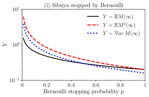
Figure 1: The plot shows the infinite time limits of (68) in log scale for a Sibuya process (with index $\mu=0.2$) which is stopped by a Bernoulli process with success probability $p$.

(ii) Bernoulli stops Bernoulli (both $N_{II}(t)$ and $N_{S}(t)$ are Bernoulli processes)

Let here $p_{S}$ be the success probability of $N_{S}(t)$, and $p$ that of $N_{II}(t)$. For this AP, which is clearly of type I for $p_{S}>0$, we have, considering (A.1) for $\mathcal{Q}=1$, that

$$\mathbb{E}M(\infty)=\frac{p}{p_{S}},\hskip 14.22636pt\mathbb{E}M^{2}(\infty)=\frac{p[1+q_{S}(p-q)]}{p_{S}^{2}}\hskip 14.22636pt\mathbb{V}\text{ar}M(\infty)=\frac{p[q+q_{S}(p-q)]}{p_{S}^{2}}.$$ (69)

We depict the behavior of these quantities in Fig. 2.

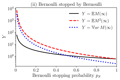
Figure 2: The figure shows the quantities of (69) in log scale. Here a Bernoulli process $N_{II}(t)$ (with success probability $p=0.6$) is stopped by another independent Bernoulli process $N_{S}(t)$ with success probability $p_{S}$.

The curves in Fig. 2 look rather similar as those in Fig. 1 with monotonous decay for increasing values of $p_{S}$ and the singularity at the type II limit for $p_{S}\to 0+$. Be aware that the values in Fig. 1 are much smaller than those in Fig. 2. This can be understood by considering the fact that, due to the long waiting times, the Sibuya process produces fewer events than a Bernoulli process until the stopping time.

3.1.3 Non-geometric absorbing time

(iii) Poisson distributed stopping time ($N_{II}(t)$ is a Bernoulli process and $\psi_{S}(t)$ is Poisson$(\lambda)$, $t\in\mathbb{N}$)

Recall $\psi_{S}(t)=\frac{\lambda^{t-1}}{(t-1)!}e^{-\lambda}$, $t\in\mathbb{N}$. The stopping time GF is ${\bar{\psi}}_{S}(u)=ue^{\lambda(u-1)}$, $|u|<1$, thus from (47),

$$\mathbb{E}M(\infty)=p\frac{d}{du}[ue^{\lambda(u-1)}]\bigg{|}_{u=1}=p(\lambda+1),\hskip 8.5359pt\mathbb{E}M^{2}(\infty)=p\left[p(\lambda+1)^{2}+\lambda+q\right].$$ (70)

Hence, the variance of $M(\infty)$ reads $\mathbb{V}\text{ar}M(\infty)=p(\lambda+q)$. Formulas (70) contain as a special case for $p=1$ the corresponding quantities of $N_{S}(t)$.

On the other hand, the limit which corresponds to stopping the Bernoulli process at $t=1$ a.s. is $\lambda\to 0+$, where the formulas in (70) boil down to (58) and (59). These asymptotic values increase monotonically as the mean stopping time of $\Delta T$ increases, that is the broader $\psi_{S}(t)$ the longer $N_{II}(t)$ remains unstopped.

3.2 Defective absorbing time

So far we assumed that $N_{S}(t)$ is of type II, that is $\psi_{S}(t)$ is non-defective. In this section we consider the absorbing time $\Delta T$ to be a defective random variable, i.e. $N_{S}(t)$ is of type I. Recall that

$$\Phi_{S}^{(0)}(t)=\mathbb{E}\,{\bf 1}_{N_{S}(t)=0}=\mathbb{E}\Theta(\Delta T-1-t)=1-\mathcal{Q}_{S}+\sum_{r=t+1}^{\infty}\psi_{S}(r)=1-\sum_{r=1}^{t}\psi_{S}(r)$$ (71)

with the large time limit

$$\Phi_{S}^{(0)}(\infty)=\lim_{t\to\infty}\mathbb{P}[\Delta T>t]=1-\sum_{r=1}^{\infty}\psi_{S}(r)=1-{\cal Q}_{S},\hskip 28.45274pt{\cal Q}_{S}\in(0,1]$$ (72)

denoting the probability that $N_{S}(\infty)=0$ (i.e. $\Delta T=\infty$). Equation (71) is the consequence of the following proposition that holds for possibly defective RVs supported on the positive integers.

Proposition 3.10.

Let $\Delta T$ be a discrete random variable with $\mathbb{P}[\Delta T=r]=\psi_{S}(r)$, $r\in\mathbb{N}$, and $(0,1]\ni{\cal Q}_{S}=\sum_{r=1}^{\infty}\psi_{S}(r)$. Then

$$\mathbb{E}f(\Delta T)=\sum_{r=1}^{\infty}\psi_{S}(r)f(r)+(1-{\cal Q}_{S})f(\infty)$$ (73)

for suitable measurable functions $f(r)$ where $f(\infty)=\lim_{r\to\infty}f(r)$.

This proposition accounts for the fact that a probability mass $1-{\cal Q}_{S}$ is located at infinity. The non-defective case appears for ${\cal Q}_{S}=1$. This relation yields infinity for the expected waiting time $\mathbb{E}\Delta T$ when $\Delta T$ is defective. Considering $f(r)=u^{r}$, $|u|\leq 1$, in (73) yields

$$\mathbb{E}u^{\Delta T}=\left\{\begin{array}[]{ll}{\bar{\psi}}_{S}(u),&|u|<1\\ \\ 1,&u=1\end{array}\right.$$ (74)

which is discontinuous at $u=1$ for $\mathcal{Q}_{S}\neq 1$, namely

$${\bar{\psi}}_{S}(u)\big{|}_{u=1}=\mathbb{E}u^{\Delta T}\big{|}_{u=1-}={\cal Q}_{S}.$$ (75)

It is then straightforward to recover the GF

$${\bar{\Phi}}_{S}^{(0)}(u)=\frac{1-\mathbb{E}u^{\Delta T}}{1-u}=\frac{1-{\bar{\psi}}_{S}(u)}{1-u},\hskip 28.45274pt|u|<1,$$ (76)

which has the same structure as (23) but this time with the property in (75). From (76) we obtain

$$\Phi_{S}^{(0)}(\infty)=(1-u){\bar{\Phi}}_{S}^{(0)}(u)\big{|}_{u=1}=1-\mathbb{E}u^{\Delta T}\big{|}_{u=1-}=1-{\bar{\psi}}_{S}(1)=1-{\cal Q}_{S}.$$ (77)

Proposition 3.10 leads to the following extension of Theorem 3.4 for the defective case.

Theorem 3.11.

Let $M(t)$ be defined as in (15), and $\psi_{S}(r)$ be defective with $\sum_{r=1}^{\infty}\psi_{S}(r)=\mathcal{Q}_{S}\in(0,1]$. Then, the PDF of $M(t)$ reads

$$\mathbb{P}[M(t)=m]=(1-\mathcal{Q}_{S})\Phi_{II}^{(m)}(t)+\sum_{r=1}^{\infty}\psi_{S}(r)\left(\Phi_{II}^{(m)}(t)\Theta(r-t-1)+\Phi_{II}^{(m)}(r)\Theta(t-r)\right).$$ (78)

Proof.

Recalling

$$\mathbb{P}[M(t)=m]=\Phi_{S}^{(0)}(t)\Phi_{II}^{(m)}(t)+\sum_{r=1}^{t}\psi_{S}(r)\Phi_{II}^{(m)}(r),$$ (79)

the result follows from Theorem 3.4 taking into account (71). ∎

We observe that the normalization condition (Corollary 3.5) remains true when the stopping time is defective

$$\sum_{m=0}^{\infty}\mathbb{P}[M(t)=m]=\Phi_{S}^{(0)}(t)+\sum_{r=1}^{t}\psi_{S}(r)=1$$ (80)

by virtue of (71) and $\sum_{m=0}^{\infty}\Phi_{II}^{(m)}(t)=1$. The probability that $M(t)$ exceeds $m_{0}$, with $m_{0}\in\mathbb{N}_{0}$, then writes

$$\begin{array}[]{clr}\displaystyle\mathbb{P}[M(t)>m_{0}]&=\displaystyle\mathbb{E}\Theta(\Delta T-1-t)\mathbb{E}\Theta(t-J_{m_{0}+1})+\mathbb{E}\Theta(t-\Delta T)\Theta(\Delta T-J_{m_{0}+1})&\\ &=\displaystyle\Phi_{S}^{(0)}(t)\mathbb{P}[N_{II}(t)>m_{0}]+\sum_{r=1}^{t}\psi_{S}(r)\mathbb{P}[N_{II}(r)>m_{0}].&\end{array}$$ (81)

The infinite time limit yields

$$\mathbb{P}[M(\infty)>m_{0}]=\Phi_{S}^{(0)}(\infty)\mathbb{P}[N_{II}(\infty)>m_{0}]+\sum_{r=1}^{\infty}\psi_{S}(r)\mathbb{P}[N_{II}(r)>m_{0}]$$ (82)

where in the second term we used

$$\lim_{t\to\infty}\mathbb{E}\Theta(t-\Delta T)f(\Delta T)=\lim_{t\to\infty}\left\{\sum_{r=1}^{t}\psi_{S}(r)f(r)+\Theta(t-\infty)f(\infty)\right\}=\sum_{r=1}^{\infty}\psi_{S}(r)f(r)$$ (83)

with $\lim_{t\to\infty}\Theta(t-\infty)=\lim_{t\to\infty}\{\lim_{r\to\infty}\Theta(t-r)\}=0$ where first we let $r\to\infty$ while $t$ is kept constant to apply Theorem 3.11 and then we consider $t\to\infty$.

Since $N_{II}(t)$ is of type II we know that $\lim_{t\to\infty}\mathbb{P}[N_{II}(t)>m_{0}]=1$. Since $\Phi_{S}^{(0)}(\infty)=1-{\cal Q}_{S}$, the probability that $M(t)$ is never stopped reads

$$\Lambda_{M}=\lim_{m_{0}\to\infty}\mathbb{P}[M(\infty)>m_{0}]=1-{\cal Q}_{S}+\lim_{m_{0}\to\infty}\sum_{r=1}^{\infty}\psi_{S}(r)\mathbb{P}[N_{II}(r)>m_{0}].$$ (84)

Now take into account that $\mathbb{P}[N_{II}(t)>m_{0}]=0$ for $t\leq m_{0}$ as $N_{II}(t)\leq t$. Therefore,

$$\sum_{r=1}^{\infty}\psi_{S}(r)\mathbb{P}[N_{II}(r)>m_{0}]=\sum_{r=m_{0}+1}^{\infty}\psi_{S}(r)\mathbb{P}[N_{II}(r)>m_{0}]\leq\sum_{r=m_{0}+1}^{\infty}\psi_{S}(r)={\cal Q}_{S}-\sum_{r=1}^{m_{0}}\psi_{S}(r)$$ (85)

and hence

$$\Phi_{S}^{(0)}(\infty)=1-{\cal Q}_{S}\leq\Lambda_{M}\leq\lim_{m_{0}\to\infty}\bigg{[}1-\sum_{r=1}^{m_{0}}\psi_{S}(r)\bigg{]}=\lim_{m_{0}\to\infty}\Phi_{S}^{(0)}(m_{0})=1-{\cal Q}_{S}$$ (86)

thus $\Lambda_{M}=1-{\cal Q}_{S}$.

The previous result suggests the following interpretation (see Remark 2.2).

• If $N_{S}(t)$ is of type I (i.e. the absorbing time is defective), $M(t)$ is an IAP and it is never stopped with probability $\Lambda_{M}=1-{\cal Q}_{S}=\Phi_{S}^{(0)}(\infty)<1$;

• If $N_{S}(t)$ is of type II (non-defective absorbing time), we have $\Lambda_{M}=0$, $M(t)$ is stopped almost surely and hence it is of type I;

• In the extremely defective limit ${\cal Q}_{S}\to 0+$, $M(t)$ is of type II (see (15)) and $\Lambda_{M}\to 1-$.

3.2.1 Defective geometric absorbing time

Here we consider $N_{S}(t)$ to be of type I. In particular it is the defective Bernoulli process (DBP) which we introduce in Appendix A.1. The DBP has the following waiting time PDF $\psi_{S}(t)=\mathcal{Q}_{S}pq^{t-1}$ where $\mathcal{Q}_{S}\in(0,1]$. Then, as mentioned above, $M(t)$ is an IAP which is not stopped with probability $\Lambda_{M}=1-\mathcal{Q}_{S}$. If $\mathcal{Q}_{S}\to 1-$ then $M(t)$ is of type I, whilst if $\mathcal{Q}_{S}\to 0+$ then $M(t)$ if of type II. The state probabilities (78) and their GF read

$$P_{m}(t)=(\Lambda_{M}+\mathcal{Q}_{S}q^{t})\Phi_{II}^{(m)}(t)+\mathcal{Q}_{S}\frac{p}{q}\left[-\delta_{m,0}+\sum_{r=0}^{t}q^{r}\Phi_{II}^{(m)}(r)\right],$$ (87)

$${\bar{P}}_{m}(u)=\Lambda_{M}\frac{1-{\bar{\psi}}_{II}(u)}{1-u}[{\bar{\psi}}_{II}(u)]^{m}+\frac{\mathcal{Q}_{S}}{q(1-u)}\left([1-{\bar{\psi}}_{II}(qu)][{\bar{\psi}}_{II}(qu)]^{m}-p\delta_{m,0}\right),$$ (88)

where (87) and (88) respectively specialize to (60) and (61) for $\mathcal{Q}_{S}=1$.

Of interest is the infinite time limit

$$P_{m}(\infty)=(1-u){\bar{P}}_{m}(u)\bigg{|}_{u=1}=\frac{\mathcal{Q}_{S}}{q}[1-{\bar{\psi}}_{II}(q)][{\bar{\psi}}_{II}(q)]^{m}-\mathcal{Q}_{S}\frac{p}{q}\delta_{m,0}$$ (89)

where the first term in (88) necessarily yields zero and for $\mathcal{Q}_{S}=1$ (89) recovers (50). The following feature appears noteworthy. Since for any finite $t$, $\sum_{m=0}^{\infty}P_{m}(t)=1$,

$$\lim_{t\to\infty}\sum_{m=0}^{\infty}P_{m}(t)=1\neq\sum_{m=0}^{\infty}P_{m}(\infty)=\mathcal{Q}_{S}.$$ (90)

The reason for the difference lies in relation (73).

Summing up (88) over $m$ takes us to the GF of the state polynomial ${\bar{\Pi}}_{\text{\it IAP}}(v,u)=\sum_{t=0}^{\infty}u^{t}\mathbb{E}v^{M(t)}$ which yields

$${\bar{\Pi}}_{\text{\it IAP}}(v,u)=\Lambda_{M}{\bar{\cal P}}_{II}(v,u)+\frac{\mathcal{Q}_{S}}{q(1-u)}\left(\frac{1-{\bar{\psi}}_{II}(qu)}{1-v{\bar{\psi}}_{II}(qu)}-p\right),\hskip 28.45274pt|v|\leq 1,|u|<1$$ (91)

where ${\bar{\cal P}}_{II}(v,t)$ is the GF (21) associated to $N_{II}(t)$. For $\mathcal{Q}_{S}\to 1-$, (91) reduces to (64) for the type I process $M(t)$.

Of interest is the large time asymptotics

$$\mathbb{E}v^{M(\infty)}=\lim_{t\to\infty}\Pi_{\text{\it IAP}}(v,t)=\lim_{u\to 1-}(1-u){\bar{\Pi}}_{\text{\it IAP}}(v,u)=\frac{\mathcal{Q}_{S}}{q}\left(\frac{1-{\bar{\psi}}_{II}(q)}{1-v{\bar{\psi}}_{II}(q)}-p\right),\quad|v|\leq 1.$$ (92)

The non-negativity of this expression can be easily seen from ${\cal\psi}_{II}(q)<q$, $q\in(0,1)$. This result remains true for complex $v=e^{i\varphi}$, $\varphi\in(0,2\pi)$, whereas for $v=1$ and taking into account (91), we have that the limit $\lim_{t\to\infty}\Pi_{\text{\it IAP}}(1,t)=1$. Furthermore, (92) retrieves (53) for $\mathcal{Q}_{S}=1$.
In the following examples we will consider the first two moments of $M(t)$ whose GFs take the general forms

$$\overline{\mathbb{E}{M}}(u)=\frac{\partial}{\partial v}{\bar{\Pi}}_{\text{\it IAP}}(v,u)\bigg{|}_{v=1}=\frac{1}{1-u}\left(\Lambda_{M}\frac{{\bar{\psi}}_{II}(u)}{1-{\bar{\psi}}_{II}(u)}+\frac{\mathcal{Q}_{S}}{q}\frac{{\bar{\psi}}_{II}(qu)}{1-{\bar{\psi}}_{II}(qu)}\right),$$ (93)

$$\overline{\mathbb{E}{M^{2}}}(u)=\Lambda_{M}\frac{{\bar{\psi}}_{II}(u)[1+{\bar{\psi}}_{II}(u)]}{(1-u)[1-{\bar{\psi}}_{II}(u)]^{2}}+\frac{\mathcal{Q}_{S}}{q}\frac{{\bar{\psi}}_{II}(qu)[1+{\bar{\psi}}_{II}(qu)]}{(1-u)[1-{\bar{\psi}}_{II}(qu)]^{2}}.$$ (94)

3.2.2 Examples

(i) Defective Bernoulli stops standard Bernoulli

Let $N_{S}(t)$ be a DBP, that is with waiting time PDF $\psi_{S}(t)=\mathcal{Q}_{S}pq^{t-1}$, $\mathcal{Q}_{S}\in(0,1]$, (see Appendix A.1 for an outline of its essential features) and let $N_{II}(t)$ be a standard Bernoulli process, independent of $N_{S}(t)$, with success probability $p_{0}$ (and $q_{0}=1-p_{0}$). The state polynomial of $N_{II}(t)$ is known to be ${\cal P}_{II}(v,t)=(p_{0}v+q_{0})^{t}$, $t\in\mathbb{N}_{0}$. Thus, the GF (91) reads

$${\bar{\Pi}}_{{\text{\it IAP}}}(v,u)=\frac{\Lambda_{M}}{1-u{\cal A}(v)}+\frac{\mathcal{Q}_{S}}{1-q{\cal A}(v)}\left(\frac{p{\cal A}(v)}{1-u}+\frac{1-{\cal A}(v)}{1-uq{\cal A}(v)}\right)$$ (95)

where we have set ${\cal A}(v)=p_{0}v+q_{0}={\cal P}_{II}(v,1)$. The state polynomial then writes

$$\displaystyle\Pi_{{\text{\it IAP}}}(v,t) =\displaystyle\mathbb{E}v^{M(t)}=(\Lambda_{M}+\mathcal{Q}_{S}q^{t}){\cal A}(v)^{t}+\frac{\mathcal{Q}_{S}p{\cal A}(v)}{1-q{\cal A}(v)}[1-q^{t}{\cal A}(v)^{t}]$$

$$=\displaystyle\Lambda_{M}{\cal A}(v)^{t}+\frac{\mathcal{Q}_{S}}{1-q{\cal A}(v)}\left(p{\cal A}(v)+(1-{\cal A}(v))q^{t}{\cal A}(v)^{t}\right)$$ (96)

with $\Pi_{{\text{\it IAP}}}(1,t)=1$ and $\Pi_{{\text{\it IAP}}}(v,0)=1$. Observe that the process $M(t)$ is not Markovian. Actually, it is not even in the non-defective case. Indeed, consider the type I limit $\mathcal{Q}_{S}=1$, i.e. when both $N_{S}$ and $N_{II}$ are standard Bernoulli processes. That $M(t)$ is not Markovian can be seen from $\Pi_{{\text{\it IAP}}}(v,t)\Pi_{{\text{\it IAP}}}(v,1)\neq\Pi_{{\text{\it IAP}}}(v,t+1)$, that violates the Markov condition. In particular, $\Pi_{{\text{\it IAP}}}(v,1)={\cal A}(v)$ is a function of the Bernoulli parameter $p_{0}$ of $N_{II}(t)$ only, and not of the stopping probability $p$ of $N_{S}(t)$. This is because no matter whether $N_{II}$ is stopped at $t=1$ or not, we have $M(1)=N_{II}(1)$ a.s., and the latter is independent of $N_{S}$, see (15). This does not hold true for $t\geq 2$, as $\Pi_{{\text{\it IAP}}}(v,t)$ is a function of both the parameters of $N_{II}$ and of $N_{S}$. Hence ${\cal A}(v)^{2}\neq\Pi_{{\text{\it IAP}}}(v,2)$, i.e. $M(t)$ is not Markovian (except for the special case $\mathcal{Q}_{S}=0$).
For $|v|<1$ ($|{\cal A}(v)|<1$) we have the stationary value

$$\Pi_{{\text{\it IAP}}}(v,\infty)=\frac{\mathcal{Q}_{S}p{\cal A}(v)}{1-q{\cal A}(v)}$$ (97)

retrieving (92). If $\mathcal{Q}_{S}=p=1$, i. e. $N_{S}(t)=t$, ($M(t)$ is stopped at $t=1$ a.s.) the stationary value is taken already at $t=1$ with $\Pi_{{\text{\it IAP}}}(v,\infty)=\mathbf{E}v^{N_{II}(1)}=\mathcal{A}(v)$. Clearly (3.2.2) is strictly positive for $v\in[0,1]$ and

$$\Pi_{{\text{\it IAP}}}(v,t)\bigg{|}_{v=0}=\mathbb{P}[M(t)=0]=\Lambda_{M}q_{0}^{t}+\frac{\mathcal{Q}_{S}}{1-qq_{0}}\left(pq_{0}+p_{0}q^{t}q_{0}^{t}\right)$$ (98)

consistently with (87) and considering the initial condition $\mathbb{P}[M(0)=0]=1$. We point out that the state polynomial (3.2.2) is an absolutely monotonic (AM) and non-decreasing function with respect to $v$, i.e. for $n\in\mathbb{N}_{0}$,

$$\frac{\partial^{n}}{\partial v^{n}}\Pi_{{\text{\it IAP}}}(v,t)\geq 0.$$ (99)

From the relation between AM functions and CM functions [5], the non-negativity of the state probabilities and moments of $M(t)$ follows. The absolute monotonicity can be easily verified in (3.2.2) as $\frac{1-q^{t}{\cal A}(v)^{t}}{1-q{\cal A}(v)}=\sum_{r=0}^{t-1}q^{r}{\cal A}(v)^{r}$ and taking into account that $q^{r}{\cal A}(v)^{r}$ belongs to the AM class. Now, let us consider the first two moments. We have

$$\mathbb{E}M(t)=\frac{\partial}{\partial v}\Pi_{{\text{\it IAP}}}(v,t)\bigg{|}_{v=1}=\Lambda_{M}p_{0}t+\frac{\mathcal{Q}_{S}p_{0}}{p}(1-q^{t}):=\Lambda_{M}p_{0}t+\mathcal{Q}_{S}B(t),\qquad\mathbb{E}M(0)=0.$$ (100)

For large times the dominating term in the first moment is $\Lambda_{M}\mathbb{E}N_{II}(t)=\Lambda_{M}p_{0}t$ as $N_{II}(t)$ is eventually not stopped with probability $\Lambda_{M}$. We depict $\mathbb{E}M(t)$ in Fig. 3 for several values of $\mathcal{Q}_{S}$.

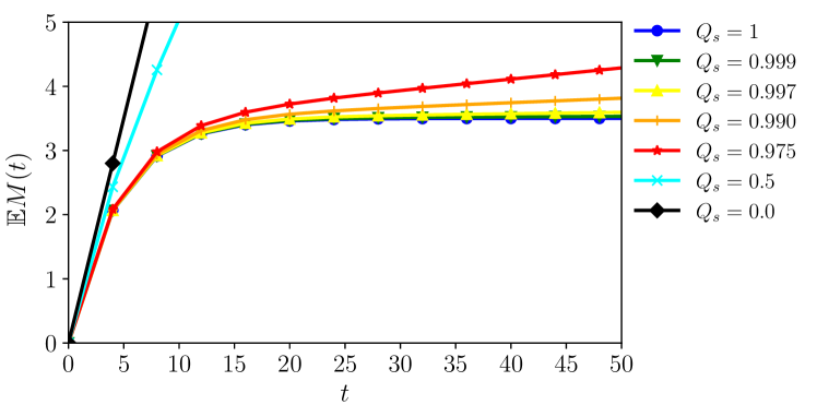
Figure 3: $\mathbb{E}M(t)$ from (100) for several values of $\mathcal{Q}_{S}$ and with parameters $q_{0}=0.3$, $q=0.8$. For large times $\mathbb{E}M(t)$ behaves linearly. In particular, for $\mathcal{Q}_{S}=1$ (type I limit) the finite asymptotic value $\mathbb{E}M(\infty)=p_{0}/p=3.5$ is approached.

The second moment reads

$$\displaystyle\mathbb{E}M^{2}(t) = \displaystyle\left(\frac{\partial^{2}}{\partial v^{2}}+\frac{\partial}{\partial v}\right)\Pi_{\textbf{\it IAP}}(v,t)\bigg{|}_{v=1}$$ (101)

$$= \displaystyle\Lambda_{M}(p_{0}^{2}t^{2}+p_{0}q_{0}t)+\mathcal{Q}_{S}\left(\frac{2p_{0}^{2}q}{p^{2}}(1-q^{t}-ptq^{t-1})+\frac{p_{0}}{p}(1-q^{t})\right)$$

$$:= \displaystyle\Lambda_{M}(p_{0}^{2}t^{2}+p_{0}q_{0}t)+\mathcal{Q}_{S}C(t).$$

We are now ready to calculate the variance:

$$\displaystyle\mathbb{V}\text{ar}{M(t)} =\Lambda_{M}\left[\mathcal{Q}_{S}p_{0}^{2}t^{2}+p_{0}q_{0}t\right]-2\Lambda_{M}\mathcal{Q}_{S}p_{0}tB(t)+\mathcal{Q}_{S}\left[C(t)-\mathcal{Q}_{S}B^{2}(t)\right]$$

$$=\displaystyle C(t)-B^{\,2}(t)+\Lambda_{M}[2B(t)(B(t)-p_{0}t)-C(t)+p_{0}^{2}t^{2}+p_{0}q_{0}t]-\Lambda_{M}^{\,2}\,(p_{0}t-B(t))^{2}.$$ (102)

The main feature is that the variance of $M(t)$ exhibits a $t^{2}$-behavior for large times (in contrast to the linear behavior of the unstopped Bernoulli emerging for $\Lambda_{M}=1$). This result can be interpreted that the defective Bernoulli stopping process introduces large fluctuations. In Fig. 4 we depict the variance (3.2.2) for several values of the defect parameter $\mathcal{Q}_{S}$ starting from $\mathcal{Q}_{S}=1$ for which $M(t)$ is of type I and is eventually stopped, and the variance has a finite asymptotic value. For decreasing $\mathcal{Q}_{S}$, the process $N_{S}(t)$ struggles to stop $N_{II}(t)$. For $\mathcal{Q}_{S}\to 0+$ the linear behavior of the standard Bernoulli $N_{II}(t)$ emerges (black line). In expression (3.2.2) one can see that the coefficient $\Lambda_{M}\mathcal{Q}_{S}$ of the term $t^{2}$ has its maximum value for $\Lambda_{M}=\mathcal{Q}_{S}=\frac{1}{2}$ where the intermediate feature of $M(t)$ is most pronounced and $\mathbb{V}\text{ar}M(t)\sim\frac{p_{0}^{2}}{4}t^{2}$. In general, the variance $\mathbb{V}\text{ar}M(t)$ is a parabolic function of $\Lambda_{M}$. The value of $\Lambda_{M}$ maximizing $\mathbb{V}\text{ar}M(t)$ turns out to be

$$\Lambda_{M,\max}(t)=\frac{1}{2[p_{0}t-B(t)]^{2}}\left[p_{0}^{2}t^{2}+p_{0}q_{0}t-C(t)+2B(t)(B(t)-p_{0}t)\right],\qquad t\geq 2,$$ (103)

where the asymptotic value $\Lambda_{M,\max}(t)$ is independent of $q$ and $q_{0}$ for $t\to\infty$ and rapidly approaches $1/2$ (Fig. 5). Hence, in this case we identify the IAP $M(t)$ with $\Lambda_{M}=1/2$ as the most fluctuating one in the long time limit. The strongly fluctuating large time behavior for $\Lambda_{M}=1/2$ can be interpreted by the ‘struggle’ of $M(t)$ to be or not to be stopped, where sample paths asymptotically approaching finite and infinite values occur with equal probability. We depict the time dependence of the variance for $\Lambda_{M}=1/2$ in Fig. 4 (cyan curve), and of $\Lambda_{M,\max}(t)$ in Fig.5. This suggests that IAPs exhibit large fluctuations in the large time limit.

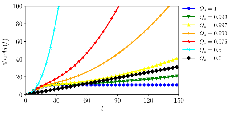
Figure 4: The variance (3.2.2) as a function of time for several choices of $\mathcal{Q}_{S}$. We have chosen here in all curves $q_{0}=0.3$ as the parameter of the standard Bernoulli $N_{II}(t)$. The stopping DPB $N_{S}(t)$ has parameter $q=0.8$. For $\mathcal{Q}_{S}=1$ (blue curve) the AP $M(t)$ is of type I and the variance has the finite asymptotic value $\mathbb{V}\text{ar}M(\infty)=\frac{2p_{0}^{2}q}{p^{2}}+\frac{p_{0}}{q}\approx 10.85$. For $\mathcal{Q}_{S}=0$ we have a type II limit $M(t)=N_{II}(t)$ with linear increase of the variance. For $\mathcal{Q}_{S}\in(0,1)$ the variance exhibits second-order large time asymptotics corresponding to large fluctuations which are most pronounced in the case $\mathcal{Q}_{S}=1/2$ (cyan curve).

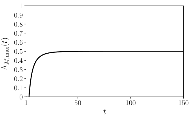
Figure 5: Time dependence of $\Lambda_{M,\max}(t)$ (formula (103)) for which the fluctuations (variance (3.2.2)) take a maximum. We observe that the asymptotic value $1/2$ is rapidly approached. The other parameters are $q_{0}=0.3$ and $q=0.8$ as in Fig. 4.

(ii) IAPs and discrete Bernstein functions

We assume that the PDF $\psi_{S}(r)$ is a superposition of geometric densities $pq^{r-1}$ where we put for our convenience $p=1-e^{-\lambda}$, $\lambda\in(0,\infty)$, namely

$$\psi_{S}(r)=\int_{0}^{\infty}(1-e^{-\lambda})e^{-\lambda(r-1)}\,a({\rm d}\lambda),\hskip 28.45274ptr\in\mathbb{N}.$$ (104)

Here $a$ is a probability measure on $\mathbb{R}_{+}$, which we allow to be defective. Equation (104) can be read as a linear combination $\psi_{S}(r)={\hat{a}}(r-1)-{\hat{a}}(r)$ of Laplace transforms

$${\hat{a}}(t)=\int_{0}^{\infty}e^{-\lambda t}a({\rm d}\lambda).$$ (105)

The normalization directly follows:

$$\sum_{r=1}^{\infty}\psi_{S}(r)=\int_{0}^{\infty}a({\rm d}\lambda)={\cal Q}_{S}$$ (106)

where ${\cal Q}_{S}<1$ if $N_{S}(t)$ is of type I (which corresponds to $a$ being defective). In the case ${\cal Q}_{S}=1$ the stopping process $N_{S}(t)$ is of type II (and $a$ then is non-defective).

Remark 3.12.

Note that $\psi_{S}(r)=\mathbb{E}\bigl{(}\mathbb{P}[Y(1)=r]\bigr{)}$, where $(Y(\tau))_{\tau\in\mathbb{R}_{+}}$ is a pure birth process in continuous time, independent of $N_{S}(t)$ and $N_{II}(t)$, and with random individual birth rate with distribution $a$.

Let us briefly highlight the connections of (104) with discrete versions of Bernstein functions and discrete complete monotonicity [45, 49]. To this end, let us introduce the discrete difference operator $D=1-{\cal T}_{-1}$ with ${\cal T}_{-r}f(t)=f(t-r)$, where $t,r\in\mathbb{Z}$.

Definition 3.13.

We call a causal discrete function $f(t)\geq 0$, $t\in\mathbb{N}_{0}$, ‘discrete completely monotone’ (DCM) if

$$(-1)^{n}D^{n}f(t)\geq 0,\hskip 28.45274ptt\geq n,\hskip 28.45274ptn\in\mathbb{N}_{0}$$ (107)

and ‘discrete Bernstein’ (DB) if

$$(-1)^{n-1}D^{n}f(t)\geq 0,\hskip 28.45274ptt\geq n,\hskip 28.45274ptn\in\mathbb{N}.$$ (108)

A basic DCM function is $e^{-\lambda t}$ for $\lambda\geq 0$. Indeed, $(-1)^{n}D^{n}e^{-\lambda t}=(e^{\lambda}-1)^{n}e^{-\lambda t}$ (remaining causal for $t\geq n$). Then, we can infer that any superposition for positive $\lambda$ is DCM, namely

$$g(t)=\int_{0}^{\infty}e^{-\lambda t}\nu({\rm d}\lambda)$$ (109)

for any integrable non-negative measure $\nu({\rm d}\lambda)$ (see e.g. [1]). This representation of DCM functions can be seen as the discrete version of Bernstein’s theorem (also known as Hausdorff–Bernstein–Widder theorem), which justifies (104) where $\psi_{S}(r)$ is in the class of DCM functions. This remains true in both the defective and non-defective cases. It is worthy of mention that the cumulative distribution function

$$1-\Phi_{S}^{(0)}(t)=\sum_{r=1}^{t}\psi_{S}(r)=\int_{0}^{\infty}(1-e^{-t\lambda})\,a({\rm d}\lambda),\hskip 28.45274ptt\in\mathbb{N}_{0}$$ (110)

is a DB function because so is $(1-e^{-t\lambda})$, and that $\Phi_{S}^{(0)}(t)$ is a DCM function. Moreover, (110) is in fact the Lévy–Khintchine representation of the DB function $1-\Phi_{S}^{(0)}(t)$ where $a$ represents the corresponding Lévy measure.
Plugging (104) into (84), and recalling (11) leads to

$$\Lambda_{M}=1-{\cal Q}_{S}+\lim_{m_{0}\to\infty}\int_{0}^{\infty}e^{\lambda}\,[{\bar{\psi}}_{II}(e^{-\lambda})]^{m_{0}+1}a({\rm d}\lambda).$$ (111)

Consider now the case $a({\rm d}\lambda)=a(\lambda){\rm d}\lambda$ where $a(\lambda)$ is a defective or non-defective PDF with respect to $\lambda$. Note that $e^{\lambda}{\bar{\psi}_{II}}(e^{-\lambda})<1$ for $\lambda>0$ due to the convexity of ${\bar{\psi}_{II}}(u)$ for $u\in(0,1)$. Now, we rescale $\lambda$ as $m_{0}^{-\frac{1}{\mu}}\lambda$, $\mu\in(0,1]$, to get, as $m_{0}\to\infty$,

$$\Lambda_{M}\sim 1-{\cal Q}_{S}+\frac{1}{m_{0}^{\frac{1}{\mu}}}\int_{0}^{\infty}e^{\lambda m_{0}^{-\frac{1}{\mu}}}[{\bar{\psi}}_{II}(e^{-\lambda m_{0}^{-\frac{1}{\mu}}})]^{m_{0}}a(\lambda m_{0}^{-\frac{1}{\mu}}){\rm d}\lambda$$ (112)

with the two cases

$${\bar{\psi}}_{II}(e^{-h})=\displaystyle\left\{\begin{array}[]{l}1-A_{1}h+o(h)\\ \\ \displaystyle 1-A_{\mu}h^{\mu}+o(h^{\mu}),\hskip 28.45274pt\mu\in(0,1)\end{array}\right.\hskip 56.9055pth\to 0$$ (113)

where $A_{1},A_{\mu}>0$. The first line refers to the case in which $\psi_{II}(t)$ is light-tailed and has finite mean $A_{1}=\sum_{r=1}^{\infty}r\psi_{II}(r)$, whereas $\mu<1$ is the case of a fat-tailed $\psi_{II}(t)$ with infinite mean (such as the Sibuya distribution). We have

$$\lim_{m_{0}\to\infty}[{\bar{\psi}}_{II}(e^{-m_{0}^{-\frac{1}{\mu}}\lambda})]^{m_{0}}=\left\{\begin{array}[]{l}\displaystyle e^{-A_{1}\lambda}\\ \\ \displaystyle e^{-A_{\mu}\lambda^{\mu}},\hskip 28.45274pt\mu\in(0,1).\end{array}\right.$$ (114)

Now we assume in (104) the following density:

$$a_{\gamma,\zeta}(\lambda)=e^{-\zeta\lambda}\frac{\lambda^{\gamma-1}}{\Gamma(\gamma)},\hskip 28.45274pt\zeta\geq 1,\hskip 14.22636pt\gamma>0$$ (115)

which is a defective PDF for $\zeta>1$ with ${\cal Q}_{S}=\zeta^{-\gamma}$ and is a $\Gamma$-distribution for $\zeta=1$. In the range $\gamma\in(0,1)$, the density (115) is weakly singular at $\lambda=0+$ with $a_{\gamma}(\lambda)\sim\frac{\lambda^{\gamma-1}}{\Gamma(\gamma)}$. From (104) we get

$$\psi_{S}^{(\gamma,\zeta)}(t)=\frac{1}{(t-1+\zeta)^{\gamma}}-\frac{1}{(t+\zeta)^{\gamma}},\hskip 28.45274ptt\in\mathbb{N}$$ (116)

that for $\gamma\in(0,1]$ is fat-tailed as $\psi_{S}^{(\gamma,\zeta)}(t)\sim\gamma t^{-\gamma-1}$, as $t\to\infty$ (i.e. with diverging expected absorbing time). For $\gamma>1$, $\psi_{S}^{(\gamma,\zeta)}(t)$, exhibits finite mean stopping time in the non-defective case $\zeta=1$. The probability that the process is not stopped up to time $t$ writes

$$\Phi_{S}^{(0),\gamma,\zeta}(t)=1-\sum_{r=1}^{t}\psi_{S}^{(\gamma,\zeta)}(r)=1-\frac{1}{\zeta^{\gamma}}+\frac{1}{(t+\zeta)^{\gamma}},\hskip 28.45274ptt\in\mathbb{N}_{0}$$ (117)

fulfilling the initial condition $\Phi_{S}^{(0),\gamma,\zeta}(t)\big{|}_{t=0}=1$ and $\lim_{t\to\infty}\Phi_{S}^{(0),\gamma,\zeta}(t)=1-\zeta^{-\gamma}$ remaining positive in the defective case.
Then, the probability that $M(t)$ is never stopped (see (14)) then reads

$$\Lambda_{M}=1-\zeta^{-\gamma}+\lim_{m_{0}\to\infty}m_{0}^{-\frac{\gamma}{\mu}}\int_{0}^{\infty}e^{-A_{\mu}\lambda^{\mu}}e^{-\lambda(\zeta-1)m_{0}^{-\frac{1}{\mu}}}\frac{\lambda^{\gamma-1}}{\Gamma(\gamma)}{\rm d}\lambda=1-\zeta^{-\gamma}=\Phi_{S}^{(0),\gamma,\zeta}(\infty)$$ (118)

where $e^{-\lambda(\zeta-1)m_{0}^{-\frac{1}{\mu}}}\to 1$. Hence, the integral converges to a constant $C=\int_{0}^{\infty}e^{-A_{\mu}\lambda^{\mu}}\frac{\lambda^{\gamma-1}}{\Gamma(\gamma)}{\rm d}\lambda$ with $\Lambda_{M}\sim 1-\zeta^{-\gamma}+m_{0}^{-\frac{\gamma}{\mu}}C$. This result covers both light- and fat-tailed $\psi_{II}(t)$ and $\psi_{S}(t)$, and is consistent with our above general result (86) with the interpretation thereafter: $M(t)$ is an IAP for $\zeta>1$, and it is a type I process for $\zeta=1$.

4 Application to random walks

4.1 General framework

Let $\vec{X}_{t}$ be the position vector of a discrete time random walk on $\mathbb{Z}^{d}$ defined as

$$\vec{X}_{t}=\sum_{r=1}^{{\cal M}(t)}\vec{\xi}_{r}=\sum_{\ell=1}^{\infty}\vec{\xi}_{\ell}\,\Theta(t-T_{\ell}),\hskip 28.45274pt\vec{X}_{0}=\vec{0},\hskip 28.45274ptt\in\mathbb{N}_{0}.$$ (119)

The walker, at $t=0$, starts at the origin. Let ${\cal M}(t)=\max(m\in\mathbb{N}_{0}:T_{m}\leq t)$ be the counting variable of a discrete-time AP with arrival times $T_{m}\in\mathbb{N}$, such as for instance the stopped AP (15). We call ${\cal M}(t)$ the generator process of the walk (119). We further assume that the steps $\vec{\xi}_{r}$ and the waiting times $T_{m}-T_{m-1}$ are independent. We note that the approach we are going to use is capable to cope with cases in which the waiting times are dependent, for instance when ${\cal M}(t)$ is not a renewal process. The steps $\vec{\xi}_{r}$ take values in $\mathbb{Z}^{d}$ and are drawn from the discrete PDF $\mathbb{P}[\vec{\xi}=\vec{y}]=\mathbb{E}\delta_{\vec{y},\vec{\xi}}=W(\vec{y})$ and are such that their first and second moments are finite. Per construction (119) is a random walk time-changed with ${\cal M}(t)$, which represents its operational time. If ${\cal M}(t)$ is a renewal process, the walk (119) is a discrete-time version of a Montroll–Weiss type walk [39]. For the following it is convenient to rewrite (119) as

$$\vec{X}_{t}=\sum_{n=0}^{\infty}\Theta(T_{n},t,T_{n+1})\sum_{r=1}^{n}\vec{\xi}_{r},$$ (120)

involving the indicator function $\Theta(T_{n},t,T_{n+1})$ (see (3.1)). Further, we denote by $\delta_{\vec{x},\vec{X}_{t}}$ the indicator function sitting at $\vec{x}$ of the position of the walker. The notation $\delta_{\vec{a},\vec{b}}=\delta_{a_{1},b_{1}}\cdot\ldots\cdot\delta_{a_{d},b_{d}}$ stands for the $d$-dimensional Kronecker symbol, where $a_{i}$ and $b_{i}$, $i\in\{1,\dots,d\}$, represent the components of the vectors $\vec{a}$ and $\vec{b}$, respectively. Then, considering the representation (120) we have

$$\delta_{\vec{x},\vec{X}_{t}}=\sum_{n=0}^{\infty}\delta_{\vec{x},\sum_{r=1}^{n}\vec{\xi}_{r}}\,\Theta(T_{n},t,T_{n+1}).$$ (121)

By taking the expectation of (121) we obtain the propagator, that is the spatial PDF $P(\vec{x},t)$ of the walker, which gives the probability of finding the walker on the lattice point $\vec{x}\in\mathbb{Z}^{d}$ at time $t$:

$$P(\vec{x},t)=\sum_{n=0}^{\infty}\mathbb{E}\Theta(T_{n},t,T_{n+1})\mathbb{E}\delta_{\vec{x},\sum_{r=1}^{n}\vec{\xi}_{r}}.$$ (122)

In (122) we used the independence between the steps $\vec{\xi}_{r}$ and the arrival process ${\cal M}(t)$. Further, the quantity $\mathbb{E}\Theta(T_{n},t,T_{n+1})=\mathbb{P}[{\cal M}(t)=n]$, the state probabilities of ${\cal M}(t)$, and $\mathbb{E}\delta_{\vec{x},\sum_{r=1}^{n}\vec{\xi}_{r}}=\mathbb{E}[\delta_{\vec{x},\vec{\xi}}\,\star]^{n}$ refers to the transition matrix of $n$ independent steps $\vec{\xi}_{r}$. The Fourier representation of the spatial PDF is

$$P(\vec{x},t) = \mathbb{E}\frac{1}{(2\pi)^{d}}\int_{-\pi}^{\pi}\ldots\int_{-\pi}^{\pi}e^{i\varphi(\vec{x}-\vec{X}_{t})\cdot\vec{\varphi}}{\rm d}\varphi_{1}\ldots{\rm d}\varphi_{d}$$ (123)

$$= \frac{1}{(2\pi)^{d}}\int_{-\pi}^{\pi}\ldots\int_{-\pi}^{\pi}e^{i\vec{\varphi}\cdot\vec{x}}{\hat{P}}(\vec{\varphi},t){\rm d}\varphi_{1}\ldots{\rm d}\varphi_{d}$$

where we used the Fourier representation of the Kronecker symbol $\delta_{r,s}=\frac{1}{2\pi}\int_{-\pi}^{\pi}e^{i\varphi(r-s)}{\rm d}\varphi$, $r,s\in\mathbb{Z}^{d}$, and wrote $\vec{a}\cdot\vec{b}=\sum_{r=1}^{d}a_{r}b_{r}$ for scalar products. The characteristic function of the random walk $\vec{X}_{t}$ is

$${\hat{P}}(\vec{\varphi},t) =\mathbb{E}e^{-i\vec{\varphi}\cdot\vec{X}_{t}}=\sum_{m=0}^{t}\mathbb{P}[{\cal M}(t)=m][{\hat{W}}(\vec{\varphi})]^{m}$$

$$=\mathcal{P}_{\mathcal{M}}({\hat{W}}(\vec{\varphi}),t)=\mathbb{E}\,{\hat{W}}(\vec{\varphi})^{\mathcal{M}(t)},\hskip 28.45274pt\varphi_{j}\in[-\pi,\pi].$$ (124)

Notice that ${\hat{P}}(\vec{\varphi},t)\big{|}_{t=0}=1$, which ensures $P(\vec{x},0)=\delta_{\vec{x},\vec{0}}$ and hence $\vec{X}_{0}=\vec{0}$ a.s., is satisfied. Further, ${\hat{P}}(\vec{\varphi},t)\big{|}_{\vec{\varphi}=\vec{0}}=1$ gives the spatial normalization of the propagator. Finally, notice the notation

$${\hat{W}}(\vec{\varphi})=\mathbb{E}e^{-i\vec{\varphi}\cdot\vec{\xi}}=\sum_{\vec{x}\in\mathbb{Z}^{d}}W(\vec{x})e^{-i\vec{\varphi}\cdot\vec{x}}.$$ (125)

Using Wald’s identity we deduce the expected position, denoting with $X_{j}(t)$ the Cartesian components of $\vec{X}_{t}$, as

$$\mathbb{E}X_{j}(t)=\mathbb{E}\mathcal{M}(t)\mathbb{E}\xi_{j}.$$ (126)

From (4.1) the second moment of the position reads

$$\mathbb{E}X_{j}(t)^{2}=\displaystyle\mathbb{E}\mathcal{M}(t)(\mathcal{M}(t)-1)[\mathbb{E}\xi_{j}]^{2}+\mathbb{E}\mathcal{M}(t)\mathbb{E}\xi_{j}^{2}=\mathbb{E}\mathcal{M}(t)^{2}[\mathbb{E}\xi_{j}]^{2}+\mathbb{E}\mathcal{M}(t)\mathbb{V}\text{ar}{\xi_{j}}$$ (127)

and therefore,

$$\mathbb{V}\text{ar}X_{j}(t)=\mathbb{V}\text{ar}{\mathcal{M}(t)}(\mathbb{E}\xi_{j})^{2}+\mathbb{E}\mathcal{M}(t)\mathbb{V}\text{ar}{\xi_{j}}.$$ (128)

The GF of the characteristic function (4.1) is

$${\hat{\bar{P}}}(\vec{\varphi},u)=\sum_{t=0}^{\infty}u^{t}{\hat{P}}(\vec{\varphi},t)=\sum_{m=0}^{\infty}{\bar{\Phi}}_{\cal M}^{(m)}(u)[{\hat{W}}(\vec{\varphi})]^{m}$$ (129)

where the GFs ${\bar{\Phi}}_{\cal M}^{(m)}(u)$ of the state probabilities $\mathbb{P}[{\cal M}(t)=m]$ of the generator process ${\cal M}(t)$ come into play.

In the following we consider a graph whose nodes constitutes a subset of $\mathbb{Z}^{d}$ and the edges are determined by the distribution of the steps $\vec{\xi}$, thus defining the topology of the graph. We assume that all the nodes of the graph have constant degree $\Lambda_{d}$.

The transition matrix for a step $\vec{x}\to\vec{x}+\vec{y}$, $\vec{x},\vec{y}\in\mathbb{Z}^{d}$, can then be represented as

$$W(\vec{y})=\mathbb{E}\delta_{\vec{y},\vec{\xi}}=\sum_{r=1}^{\Lambda_{d}}p_{r}\delta_{\vec{y},\vec{a}^{(r)}}$$ (130)

where the walker performs the step $\vec{a}^{(r)}$ with probability $p_{r}$. Note that $\delta_{\vec{y},\vec{a}}$ is the matrix describing the deterministic step $\vec{x}\to\vec{x}+\vec{a}$ and (130) averages over all possible steps. The probabilities $p_{r}$ can be conceived as the weights of the edges in a weighted graph and clearly

$$\sum_{\vec{y}\in\mathbb{Z}^{d}}W(\vec{y})=\sum_{r=1}^{\Lambda_{d}}p_{r}=1.$$ (131)

The vectors $\vec{a}^{(r)}$ represent the directed edges of the graph. This representation allows us to capture a wide range of possibly biased walks on weighted graphs (see [43, 44, 47] for related models).

In order to focus on the effects induced by the generator process ${\cal M}(t)$, we focus on simple walks in which the Fourier transform (125) takes the form

$${\hat{W}}(\vec{\varphi})=\sum_{r=1}^{\Lambda_{d}}p_{r}e^{-i\vec{\varphi}\cdot\vec{a}^{(r)}}.$$ (132)

For walks on undirected graphs (unbiased walks), all moments of odd order vanish, thus (132) is real and takes the form $W(\vec{\varphi})=\sum_{r=1}^{\Lambda_{d}}p_{r}\cos{\vec{\varphi}\cdot\vec{a}^{(r)}}$. This case includes the well-known unbiased walk on $\mathbb{Z}^{d}$ with $\Lambda_{d}=2d$ and

$${\hat{W}}(\vec{\varphi})=\frac{1}{d}\sum_{r=1}^{d}\cos{\varphi_{r}}$$ (133)

(consult for instance [42] and [21]). We study now a few cases of random walks of the form (119). We use the following classification (cf. Remark 2.2):

Definition 4.1.

• $\vec{X}_{t}$ is a type I RW if ${\cal M}(t)$ is an AP of type I;

• $\vec{X}_{t}$ is of type II RW if ${\cal M}(t)$ is an AP of type II;

• $\vec{X}_{t}$ is an intermediate random walk (IRW) if ${\cal M}(t)$ is an IAP.

In the following subsection we provide some examples of IRWs.

4.2 Intermediate random walks: defective Bernoulli stops the random walker

The aim of the present section is to analyze an IRW (119) in the case in which the generator process ${\cal M}(t)=M(t)$ is the IAP defined by (15). Here, we assume that $N_{S}(t)$ is a DBP (see Section 3.2.2 and Appendix A.1). Recall its waiting time PDF is $\psi_{S}(t)=\mathcal{Q}_{S}pq^{t-1}$, $t\in\mathbb{N}$ (and $\Lambda_{M}=1-\mathcal{Q}_{S}$). This IRW is a discrete-time version of a Montroll–Weiss walk (that is, a RW time-changed with a type II RP $N_{II}(t)$) which is stopped at the first event of an independent DBP. Using (91), the GF (129) writes

$$\displaystyle{\hat{\bar{P}}}(\vec{\varphi},u) =\displaystyle{\bar{\Pi}}_{\text{{IAP}}}({\hat{W}}(\vec{\varphi}),u)$$

$$=\displaystyle\Lambda_{M}\frac{1-{\bar{\psi}}_{II}(u)}{(1-u)[1-{\hat{W}}(\vec{\varphi}){\bar{\psi}}_{II}(u)]}+\frac{\mathcal{Q}_{S}}{q(1-u)}\left(\frac{1-{\bar{\psi}}_{II}(qu)}{1-{\hat{W}}(\vec{\varphi}){\bar{\psi}}_{II}(qu)}-p\right).$$ (134)

For $\Lambda_{M}=1$ we have the discrete-time counterpart of the Montroll–Weiss walk. If $\mathcal{Q}_{S}=1$ it is a type I RW with geometric absorbing time. Note that ${\hat{\bar{P}}}(\vec{\varphi},u)|_{\vec{\varphi}=\vec{0}}=(1-u)^{-1}$ and ${\hat{\bar{P}}}(\vec{\varphi},u)|_{u=0}=1$ are consistent with the normalization of the propagator and the initial condition $\vec{X}_{0}=\vec{0}$ a.s., respectively.

4.2.1 Example: ${N_{II}(t)}$ Bernoulli process.

Let $N_{II}(t)$ be a Bernoulli process with $\psi_{II}(t)$ with parameter $p_{0}$. Then, by using (3.2.2), the characteristic function (4.1) takes the explicit form

$${\hat{P}}(\vec{\varphi},t)=\Pi_{IAP}({\hat{W}}(\vec{\varphi}),t)=\Lambda_{M}{\cal A}^{t}+\frac{\mathcal{Q}_{S}}{1-q{\cal A}}\left(p{\cal A}+(1-{\cal A})q^{t}{\cal A}^{t}\right),\hskip 28.45274pt{\cal A}(\vec{\varphi})=q_{0}+p_{0}{\hat{W}}(\vec{\varphi}).$$ (135)

In order to explore the diffusive features of the RW, we investigate the first two moments of the position $\vec{X}_{t}$ of the walker. Recalling (100), the expected value of the $j$-th component of the position of the walker is

$$\mathbb{E}X_{j}(t)=\mathbb{E}M(t)\,\mathbb{E}\xi_{j}=\left[\Lambda_{M}p_{0}t+\frac{\mathcal{Q}_{S}p_{0}}{p}(1-q^{t})\right]\,\mathbb{E}\xi_{j}.$$ (136)

For large values of $t$, the drift of this walk is dominated by the linear contribution of the Bernoulli process $N_{II}(t)$. From (127), together with (100) and (101), the second moment of the $j$-th component of the position is

$$\displaystyle\mathbb{E}X_{j}^{2}(t)={} \displaystyle\mathbb{E}M^{2}(t)(\mathbb{E}\xi_{j})^{2}+\mathbb{E}M(t)\mathbb{V}\text{ar}\,{\xi_{j}}$$

$$={} \displaystyle\left(\Lambda_{M}(p_{0}^{2}t^{2}+p_{0}q_{0}t)+\mathcal{Q}_{S}\biggl{[}\frac{2p_{0}^{2}q}{p^{2}}(1-q^{t}-ptq^{t-1})+\frac{p_{0}}{p}(1-q^{t})\biggr{]}\right)(\mathbb{E}\xi_{j})^{2}$$

$$+\displaystyle\left(\Lambda_{M}p_{0}t+\frac{\mathcal{Q}_{S}p_{0}}{p}(1-q^{t})\right)\mathbb{V}\text{ar}\,{\xi_{j}}.$$ (137)

(i) Unbiased walk. We observe the following behavior. If the walk is unbiased (i.e. if $\mathbb{E}\xi_{j}=0$ $\forall j=1,\ldots,d$), the mean square displacement (MSD) and the variance grow linearly for large times:

$$\mathbb{E}\sum_{j=1}^{d}X_{j}^{2}(t)\sim K\,t,\qquad K=\Lambda_{M}p_{0}\sum_{j=1}^{d}\mathbb{E}\xi_{j}^{2},\qquad t\to\infty,$$ (138)

corresponding to a diffusive behavior with diffusion coefficient $K$ determined by the unbounded sample paths of $N_{II}(t)$. This implies that the asymptotics (138) does not depend on $p$. However, the diffusion coefficient $K$ decreases as $\mathcal{Q}_{S}$ approaches one, and is maximal if $\mathcal{Q}_{S}=0$.

Remark 4.2.

In the simple unbiased walk on $\mathbb{Z}^{d}$ with next neighbor steps along the edges of the d-dimensional hypercubic lattice [21], occurring with equal probability $1/(2d)$ we have $\mathbb{E}\xi_{j}=0$ and $\mathbb{E}\xi_{j}^{2}=1/d$ ($j=1,\ldots,d$). The diffusion coefficient defined in (138) then is $K=\Lambda_{M}p_{0}$. Note that different processes $N_{S}(t)$ and $N_{II}(t)$, and hence different values of $\Lambda_{M}$ and $p_{0}$, are able to reproduce the same diffusion coefficient $K$.

(ii) Biased walk. The walk is biased if $\mathbb{E}\xi_{j}\neq 0$ for at least one component $j$. From (4.2.1) we observe a ballistic superdiffusive behavior

$$\mathbb{E}X_{j}^{2}(t)\sim\Lambda_{M}p_{0}^{2}(\mathbb{E}\xi_{j})^{2}\,t^{2},\qquad t\to\infty.$$ (139)

The dominating term of the asymptotic variance of the position is quadratic and comes from the variance of the generator $M(t)$.

Next we discuss an explicit example in the $2d$ triangular lattice.

4.2.2 IRWs on the triangular lattice

We consider biased and unbiased versions of the IRW (119) on an infinite triangular lattice in the case in which the generator process ${\cal M}(t)=M(t)$ is the IAP defined by (15).

In the biased RW we allow only four steps towards neighbor lattice points $\vec{a}^{(r)}=(\cos\frac{r\pi}{3},\sin\frac{r\pi}{3})$, $r\in\{0,1,2,3\}$, each with equal probability $p_{r}=1/4$, see Fig. 6(a). In the unbiased RW steps to all the $6$ closest neighbor lattice points $\vec{a}^{(r)}$, $r\in\{0,\ldots,5\}$, occur with equal probability $p_{r}=1/6$, see Fig. 6(b).

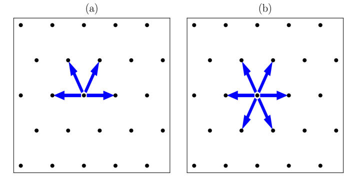
Figure 6: Blue arrows represent the allowed and equally probable steps in a biased walk (panel (a)) and in an unbiased walk (panel (b)) on the triangular lattice with lattice constant set equal to unity.

(i) Unbiased case. We have that $\mathbb{E}\xi_{j}=0$ and $\mathbb{E}(\xi_{1}^{2}+\xi_{2}^{2})=1$ thus the MSD reads

$$\sum_{j=1}^{2}\mathbb{E}X_{j}^{2}(t)=\mathbb{E}M(t).$$ (140)

In the special case of a DBP stopped by a standard Bernoulli, for large values of $t$ a diffusion behavior emerges. Namely, $\sum_{j=1}^{2}\mathbb{E}X_{j}^{2}(t)\sim\Lambda_{M}p_{0}t$, (see (100) and Fig. 3)).

(ii) Biased case. We have $\mathbb{E}\xi_{1}=0$, $\mathbb{E}\xi_{2}=\frac{\sqrt{3}}{4}$, $\mathbb{E}(\xi_{1}^{2}+\xi_{2}^{2})=1$ giving the MSD:

$$\sum_{j=1}^{2}\mathbb{E}X_{j}^{2}(t)=\frac{3}{16}\mathbb{E}M^{2}(t)+\frac{13}{16}\mathbb{E}M(t).$$ (141)

Again in the DBP stopped by a standard Bernoulli case we observe a ballistic law that is

$$\sum_{j=1}^{2}\mathbb{E}X_{j}^{2}(t)\sim\frac{3}{16}\Lambda_{M}p_{0}^{2}t^{2},\qquad t\to\infty.$$ (142)

Of some interest is also the expected position of the walker at time $t$. Since $\mathbb{E}\xi_{1}=0$ (and thus $\mathbb{E}X_{1}(t)=0$) only the second component is non-zero. In particular,

$$\mathbb{E}X_{2}(t)=\frac{\sqrt{3}}{4}\mathbb{E}M(t)\sim\frac{\sqrt{3}}{4}\Lambda_{M}p_{0}t,\qquad t\to\infty,$$ (143)

showing a linear drift. We plot the exact expression of the MSD (141) in Fig. 7 for the same values of $\mathcal{Q}_{S}$ as in Figs. 3 and 4. In the type I limit of the walk ($\mathcal{Q}_{S}=1$) the MSD has a finite asymptotic value (blue curve). One can clearly see that the smaller $\mathcal{Q}_{S}$ the stronger the MSD grows. The black line corresponds to the type II limit of the walk.

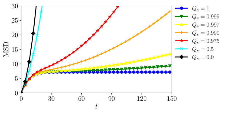
Figure 7: MSD of the RW in the biased case from (141). The parameters are chosen as in Fig. 4.

4.3 Random walks emerging from the type I limit of $M(t)$

Let us investigate now the type I limit of $M(t)$, that is when $N_{S}(t)$ is of type II. For simplicity we consider the case in which $N_{S}(t)$ is a standard Bernoulli RP and $N_{II}(t)$ is an arbitrary type II RP as considered in Section 3.1.2. This case generates a RW of type I. To this end we evaluate the characteristic function (4.1) for $t\to\infty$ (see (53):

$${\hat{P}}(\vec{\varphi},\infty)=\Pi({\hat{W}}(\vec{\varphi}),\infty)=\lim_{u\to 1-}(1-u){\hat{\bar{P}}}(\vec{\varphi},u)=-\frac{p}{q}+\frac{1-{\bar{\psi}}_{II}(q)}{q[1-{\hat{W}}(\vec{\varphi})\,{\bar{\psi}}_{II}(q)]}.$$ (144)

The quantity

$${\hat{\bar{P}}}_{q}(\vec{\varphi},u):=\frac{1-{\bar{\psi}}_{II}(qu)}{(1-u)[1-{\hat{W}}(\vec{\varphi}){\bar{\psi}}_{II}(qu)]}$$ (145)

refers to a Montroll–Weiss-type walk (119) with as a generator the renewal process ${\cal R}_{q}(t)$ with defective waiting time density $\psi_{q}(t)=\psi_{II}(t)q^{t}$ (see the end of Section 3.1.2). Propagator (4.2) (with $\Lambda_{M}=0$) then has the representation

$$P(\vec{x},t)=\frac{1}{q}P_{q}(\vec{x},t)-\frac{p}{q}\delta_{\vec{x},\vec{0}}$$ (146)

with the initial condition $P(\vec{x},t)|_{t=0}=P_{q}(\vec{x},t)|_{t=0}=\delta_{\vec{x},\vec{0}}$.

Note that for $p\in(0,1)$ the type I nature of the walk implies the existence of the stationary PDF, which reads

$$P(\vec{x},\infty)=\frac{1}{q}P_{q}(\vec{x},\infty)-\frac{p}{q}\delta_{\vec{x},\vec{0}},\hskip 28.45274pt\vec{x}\in\mathbb{Z}^{d},$$ (147)

where

$$P_{q}(\vec{x},\infty)=\frac{1-{\bar{\psi}}_{II}(q)}{(2\pi)^{d}}\int_{-\pi}^{\pi}\dots\int_{-\pi}^{\pi}\frac{e^{i\vec{\varphi}\cdot\vec{x}}}{[1-{\hat{W}}(\vec{\varphi}){\bar{\psi}}_{II}(q)]}{\rm d}\varphi_{1}\ldots{\rm d}\varphi_{d},\hskip 28.45274pt\vec{x}\in\mathbb{Z}^{d}.$$ (148)

This limit propagator describes a ‘non-equilibrium steady state’ (NESS) as known in the context of stochastic resetting, see [4, 14].

4.3.1 Continuous-space scaling limit to a universal NESS

Here, we consider a scaling limit for $p\to 0+$ where the infinite time propagator (147) boils down to (148). To do that, we introduce the scaling parameter (see (55))

$$\lambda\sim\mathbb{E}M(\infty)=\frac{{\bar{\psi}}_{II}(q)}{q[1-{\bar{\psi}}_{II}(q)]}\sim\frac{1}{1-{\bar{\psi}}_{II}(q)}\sim\frac{1}{C_{\mu}p^{\mu}}\to\infty,\qquad p\to 0+,$$ (149)

where we have used the asymptotic expansion ${\bar{\psi}}_{II}(1-p)\sim 1-C_{\mu}p^{\mu}+o(p^{\mu})$, $C_{\mu}>0$, $\mu\in(0,1]$ (see also (113)). Clearly, (147) and (148) converge to the same limiting propagator which we denote by $P_{c}(\vec{x},\infty)$. The latter is related to the asymptotic behavior of the type II auxiliary renewal process $\mathcal{R}_{q}(t)$ whose interarrival time PDF becomes non-defective for $q\to 1-$ (see (63–66).
We will see in the following that the emerging NESS is universal, in the sense that it is the same for any type II renewal process $N_{II}(t)$: it depends only on the probabilistic properties of the steps captured by ${\hat{W}}(\vec{\varphi})$.

In the following sections, we derive the NESS propagator for special classes of walks.

Light-tailed step distribution.

Here we investigate the class of walks such that the first and second step moments $A_{j}=\mathbb{E}\xi_{j}$ and $B_{j}=\mathbb{E}\xi_{j}^{2}$ are finite. For this class we have the expansion

$${\hat{W}}(\vec{\varphi})=1-i\sum_{j=1}^{d}A_{j}\varphi_{j}-\frac{1}{2}\sum_{j=1}^{d}\varphi_{j}^{2}B_{j}+\ldots,\qquad|\vec{\varphi}|\to 0.$$ (150)

In particular, we focus on the two cases of biased and unbiased walks.

(i) Biased case ($A_{j}\neq 0$ for at least one $j$).

The Fourier transform of (148) then writes

$$\frac{1}{1-\frac{{\bar{\psi}}_{II}(q)}{1-{\bar{\psi}}_{II}(q)}[{\hat{W}}(\vec{\varphi})-1]}=\frac{1}{1+\lambda[1-\hat{W}(\vec{\varphi})]}=\int_{0}^{\infty}e^{-\tau[1+\lambda[1-\hat{W}(\vec{\varphi})]}{\rm d}\tau\overset{\vec{\varphi}\to\vec{0}}{\longrightarrow}\int_{0}^{\infty}e^{-\tau(1+i\vec{k}\cdot{\vec{A}})}{\rm d}\tau$$ (151)

where $k_{j}=\lambda\varphi_{j}\in[-\pi\lambda,\pi\lambda]$ and we denote the components of the rescaled position vector by $y_{j}=x_{j}/\lambda$,  (that is $\vec{Y}\in\lambda^{-d}\mathbb{Z}^{d}\to\mathbb{R}^{d}$ as $\lambda\to\infty$, and $\lambda^{-1}$ is the rescaled lattice constant). In (151) we use

$$\lambda\left[1-{\hat{W}}\left(\frac{\vec{k}}{\lambda}\right)\right]=i\sum_{j}^{d}A_{j}k_{j}+\frac{1}{2\lambda}\sum_{j}^{d}B_{j}k_{j}^{2}+o(\lambda^{-1})\ \overset{\lambda\to\infty}{\longrightarrow}\ i\sum_{j}^{d}A_{j}k_{j}=i\vec{k}\cdot\vec{A}.$$ (152)

Note that ${\hat{W}}(\vec{k}/\lambda)=\sum_{r=1}^{\Lambda_{d}}p_{r}e^{-i\vec{k}\cdot\vec{a}_{r}/\lambda}=\mathbb{E}e^{-i\vec{k}\cdot\vec{a}^{\prime}}$ contains the rescaled steps $\vec{a}_{r}^{\prime}=\vec{a}_{r}/\lambda$. The continuous space limiting propagator yields

$$\begin{array}[]{clr}\displaystyle P_{c}(\vec{y},\infty)&=\displaystyle\lim_{\lambda\to\infty}\lambda^{d}P_{q}(\vec{x},\infty)=\displaystyle\lim_{\lambda\to\infty}\frac{1}{(2\pi)^{d}}\int_{-\lambda\pi}^{\lambda\pi}\ldots\int_{-\lambda\pi}^{\lambda\pi}\frac{e^{i\vec{k}/\lambda\cdot\vec{x}}}{1+\lambda(1-{\hat{W}}(\vec{k}/\lambda))}{\rm d}k_{1}\ldots{\rm d}k_{d}&\\ \\ &=\displaystyle\int_{0}^{\infty}{\rm d}\tau\,e^{-\tau}\frac{1}{(2\pi)^{d}}\int_{-\infty}^{\infty}{\rm d}k_{1}\ldots\int_{-\infty}^{\infty}{\rm d}k_{d}e^{i\vec{k}\cdot(\vec{y}-\tau\vec{A})}&\\ \\ &=\displaystyle\int_{0}^{\infty}{\rm d}\tau\,e^{-\tau}\delta^{d}(\vec{y}-\tau\vec{A}).&\end{array}$$ (153)

For $d=1$ we can evaluate this case explicitly, obtaining

$$P_{c}(y,\infty)\sim\frac{1}{|A|}\Theta\left(\frac{y}{A}\right)e^{-\frac{y}{A}}$$ (154)

which is a one-sided exponential PDF and is non-null only in the sense on the direction of the bias, i.e. for $\text{sgn}(y)=\text{sgn}(A)$. We plot (154) for several values of $A$ in Fig. 8. Note that $A=\mathbb{E}X_{c}(\infty)$ is the expected final position of the walk. Further, as $A$ increases, the distribution (154) becomes more spread-out.

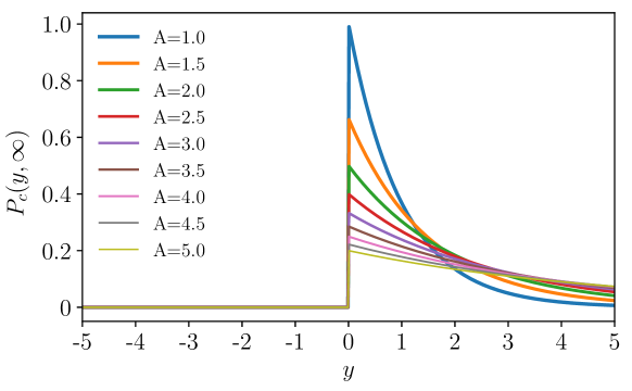
Figure 8: Limiting propagator $P_{c}(y,\infty)$ of the biased walk from (154) for different values of $A$.

(ii) Unbiased case ($A_{j}=0$ for $j=1,\ldots,d$, and $B_{j}>0$ for at least one $j$).

Differently from the biased case, we rescale the spatial coordinates as $y_{j}=x_{j}\lambda^{-1/2}$ with $\vec{Y}\in\lambda^{-d/2}\mathbb{Z}^{d}\to\mathbb{R}^{d}$, as $\lambda\to\infty$, and $k_{j}=\sqrt{\lambda}\varphi_{j}\in[-\pi\sqrt{\lambda},\pi\sqrt{\lambda}]$. The continuous space limit propagator, considering that $\lambda(1-\hat{W}(\vec{k}/\sqrt{\lambda}))\to\sum_{j=1}^{d}\frac{B_{j}}{2}k_{j}^{2}$, reads

$$\displaystyle P_{c}(\vec{y},\infty) = \displaystyle\lim_{\lambda\to\infty}\lambda^{\frac{d}{2}}P_{q}(\vec{x},\infty)$$ (155)

$$= \displaystyle\frac{1}{(2\pi)^{d}}\int_{0}^{\infty}{\rm d}\tau\,e^{-\tau}\int_{-\infty}^{\infty}{\rm d}k_{1}\ldots\int_{-\infty}^{\infty}{\rm d}k_{d}\,e^{i\vec{k}\cdot\vec{y}-\frac{\tau}{2}\sum_{j=1}^{d}B_{j}k_{j}^{2}}.$$

Note that each of the above integrals take a Gaussian form:

$$\frac{1}{2\pi}\int_{-\infty}^{\infty}e^{iky}e^{-\frac{\tau Bk^{2}}{2}}{\rm dk}=\displaystyle\frac{e^{\frac{-y^{2}}{2B\tau}}}{\sqrt{2\pi B\tau}}.$$ (156)

Therefore,

$$P_{c}(\vec{y},\infty)=\displaystyle\int_{0}^{\infty}\frac{e^{-\frac{1}{2\tau}\sum_{j=1}^{d}\frac{y_{j}^{2}}{B_{j}}}}{\sqrt{(2\pi\tau)^{d}B}}\,e^{-\tau}\,{\rm d}\tau,\hskip 28.45274ptB=\prod_{j=1}^{d}B_{j},$$ (157)

i.e. the unbiased limiting propagator turns out to be a superposition of symmetric Gaussians where $\mathbb{E}Y_{j}^{2}=B_{j}$ is retained. For $d=1$ we can evaluate this case explicitly:

$$P_{c}(y,\infty)=\frac{1}{2\pi}\int_{-\infty}^{\infty}\frac{e^{iky}}{\frac{B}{2}k^{2}+1}{\rm d}k=\frac{1}{2\pi}\int_{-\infty}^{\infty}\frac{e^{iky}}{\frac{B}{2}(k-\kappa_{1})(k-\kappa_{2})}{\rm d}k$$ (158)

with complex conjugate zeros $\kappa_{1,2}=\pm i\sqrt{\frac{2}{B}}$. Closing the integration path for $y>0$ by an infinite half circle in the upper and for $y<0$ in the lower complex plane and applying the residue theorem yields

$$P_{c}(y,\infty)=\Theta(y)\frac{2i}{B}\frac{e^{i\kappa_{1}y}}{\kappa_{1}-\kappa_{2}}-\Theta(-y)\frac{2i}{B}\frac{e^{i\kappa_{2}y}}{\kappa_{2}-\kappa_{1}}=\frac{e^{-|y|\sqrt{\frac{2}{B}}}}{\sqrt{2B}}$$ (159)

which is the PDF of a Laplace random variable with location parameter zero and scale parameter $\sqrt{B/2}$. Note that $B$ is the variance of the random walk with limiting propagator $P_{c}(y,\infty)$. In Fig. 9 we plot the propagator $P_{c}(y,\infty)$ for several values of $B$.

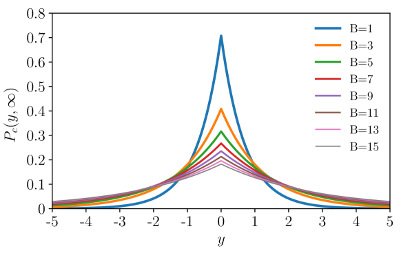
Figure 9: Limiting propagator $P_{c}(y,\infty)$ from (159) for the unbiased case for different values of $B$.

Power-law distributed steps.

We briefly explore a few cases of walks with power-law distributed steps with infinite mean or variance. We discriminate between biased and unbiased walks in $d=1$.

(a) Sibuya walk

Consider a strictly increasing walk with Sibuya distributed steps on $\mathbb{N}$ (“Sibuya walk”, see e.g. [34], Section 4). We have then, instead of (150), the characteristic function of the steps

$${\hat{W}}_{\alpha}(\varphi)=1-[1-e^{-i\varphi}]^{\alpha}\!\!,\qquad\alpha\in(0,1).$$ (160)

We introduce the scaling $k=\lambda^{\frac{1}{\alpha}}\varphi$. The rescaled walk $Y=\lambda^{-\frac{1}{\alpha}}X\in\lambda^{-\frac{1}{\alpha}}\mathbb{N}$ exhibits the essential feature,

$$\lambda[1-{\hat{W}}_{\alpha}(\lambda^{-\frac{1}{\alpha}}k)]\to(ik)^{\alpha}\!\!,\qquad\lambda\to\infty.$$ (161)

It turns out that the limiting propagator is

$$P_{c}(y,\infty)=\displaystyle\lim_{\lambda\to\infty}\lambda^{\frac{1}{\alpha}}P_{q}(x,\infty)=\int_{0}^{\infty}{\rm d}\tau e^{-\tau}\frac{1}{2\pi}\int_{-\infty}^{\infty}e^{iky}e^{-\tau(ik)^{\alpha}}{\rm d}k.$$ (162)

In formula (162), the inner integral corresponds to the one-sided stable probability density function ${\cal L}_{\alpha}(y)=\frac{1}{2\pi}\int_{-\infty}^{\infty}e^{iky}e^{-(ik)^{\alpha}}{\rm d}k$, $\alpha\in(0,1)$. This PDF is causal and has a $y^{-\alpha-1}$ fat-tailed decay for $y\to+\infty$, which entails an infinite mean. Consult [32, 48] for related models of random walks with bias.

(b) One-sided power-law steps with finite mean

If the strictly increasing walk has finite mean and infinite variance, then the characteristic function of the steps takes the form [37]

$${\hat{W}}(\varphi)=1-Ai\varphi+B_{\mu}(i\varphi)^{\mu}+o(|\varphi|^{\mu}),\qquad\mu\in(1,2)$$ (163)

with $A,B_{\mu}>0$. Due to the lowest order $i\varphi$ in this expansion, the limiting distribution coincides with (154).

A unified description of the one-dimensional case: Lévy steps.

Now we consider the canonical form of a stable density $\mathcal{L}_{\alpha}(y)$:

$${\cal L}_{\alpha}(y)=\frac{1}{2\pi}\int_{-\infty}^{\infty}e^{iky}e^{-(i^{\theta}k)^{\alpha}}{\rm d}k,\hskip 28.45274pt\alpha\in(0,2],$$ (164)

containing a further real parameter $\theta$, and where $(i^{\theta}k)^{\alpha}=|k|^{\alpha}e^{\frac{\pi i}{2}\text{sgn}(k)\alpha\theta}$. For large $|y|$ and $\alpha\in(0,2)$, ${\cal L}_{\alpha}(y)$ scales as $|y|^{-\alpha-1}$. We consider here a random walk whose characteristic function is

$${\hat{W}}_{\alpha}(\varphi)=1-(i^{\theta}\varphi)^{\alpha}+o(|\varphi|^{\alpha})$$ (165)

with index $\alpha\in(0,2]$. One can show that the previously discussed cases are contained in (165). Now, by the re scaling $k=\lambda^{\frac{1}{\alpha}}\varphi$ we obtain the Fourier transform of the NESS propagator ${\hat{P}}_{c}(k,\infty)=(1+(i^{\theta}k)^{\alpha})^{-1}$ and hence

$$P_{c}(y,\infty)=\int_{0}^{\infty}{\rm d}\tau\,e^{-\tau}\frac{1}{2\pi}\int_{-\infty}^{\infty}e^{iky}e^{-\tau(i^{\theta}k)^{\alpha}}{\rm d}k=\int_{0}^{\infty}{\rm d}\tau\,e^{-\tau}\tau^{-\frac{1}{\alpha}}\frac{1}{2\pi}\int_{-\infty}^{\infty}e^{i\kappa X/\tau^{\frac{1}{\alpha}}}e^{-(i^{\theta}\kappa)^{\alpha}}{\rm d}\kappa.$$ (166)

Formula (165) contains as a special case the class of symmetric Lévy flights for which the steps are such that ${\hat{W}}_{\alpha}(\varphi)=1-|\varphi|^{\alpha}+o(|\varphi|^{\alpha})$, that is symmetric $\alpha$-stable random variables with PDF ${\cal L}_{\alpha}(y)=\frac{1}{2\pi}\int_{-\infty}^{\infty}e^{iky}e^{-|k|^{\alpha}}{\rm d}k$. Clearly, our discussion on the case of asymptotically power-law distributed steps is not exhaustive. We refer to [9, 31] (and the references therein) for a detailed analysis of the dynamics of $\alpha$-stable propagators.

The previous construction yields to the following general expression of the NESS propagator.

Proposition 4.3.

For $d=1$ the NESS propagator (148) for $p\to 0^{+}$ takes the following form

$$P_{c}(y,\infty)=\int_{0}^{\infty}e^{-\tau}\tau^{-\frac{1}{\alpha}}{\cal L}_{\alpha}(y\tau^{-\frac{1}{\alpha}}){\rm d}\tau,\hskip 28.45274pty\in\mathbb{R},$$ (167)

written in terms of ${\cal L}_{\alpha}(y)$ that denotes a specific alpha-stable PDF which depends on the random walk (119).

Remark 4.4.

For $d=1$ ($A_{1}=A$, $y_{1}=y$) we identify (153) with (167) where we consider ${\cal L}_{1}(y)=\delta(y-A)$.
For $d=1$, (157) takes the form (167) where ${\cal L}_{2}(y)$ is Gaussian with mean zero and variance equal to $B$.
As mentioned above, for the Sibuya walk, (162) for $k^{\prime}=k\tau^{\frac{1}{\alpha}}$ gives (167) where ${\cal L}_{\alpha}(y)=\frac{1}{2\pi}\int_{-\infty}^{\infty}e^{iky}e^{-(ik)^{\alpha}}{\rm d}k$ (index $\alpha\in(0,1)$) is a one-sided stable PDF.

Appendix A Appendix

In the following appendices we consider transient arrival processes which are renewal processes with IID interarrival times having defective PDF $\psi_{I}(t)$, that is $\sum_{t=1}^{\infty}\psi_{I}(t)=\mathcal{Q}<1$.

A.1 Defective Bernoulli process (DBP)

We introduce a type I renewal process which we refer to as ‘defective Bernoulli process’ (DBP). Here we denote with $N_{I}(t)$ the DBP counting variable and define the DBP by the waiting time GF

$${\bar{\psi}}_{I}(u)=\mathcal{Q}\frac{pu}{1-qu},\hskip 28.45274ptp+q=1,\hskip 28.45274pt\mathcal{Q}\in(0,1],$$ (A.1)

of the PDF $\psi_{I}(t)=\mathcal{Q}pq^{t-1}$, $t\in\mathbb{N}$. This gives straightforwardly the survival probability

$$\Phi_{I}^{(0)}(t)=\mathcal{P}+\mathcal{Q}q^{t}$$ (A.2)

with $\mathcal{P}=1-\mathcal{Q}$ and $\Phi_{I}^{(0)}(0)=1$. The probability $\Phi_{I}^{(0)}(t)\to\mathcal{P}$ as $t\to\infty$ and it has the GF

$${\bar{\Phi}}_{I}^{(0)}(u)=\frac{\mathcal{P}}{1-u}+\frac{\mathcal{Q}}{1-qu}.$$ (A.3)

For $\mathcal{Q}=1$ all these relations turn into those of the standard Bernoulli process. Now, consider the state probabilities $\mathbb{P}[N_{I}(t)=n]=\Phi_{I}^{(n)}(t)$, i.e. the probability that $N_{I}$ counts $n$ events up to and including time $t$. Its GF reads (cf. (23))

$${\bar{\Phi}}_{I}^{(n)}(u) =\sum_{t=0}^{\infty}u^{t}\Phi_{I}^{(n)}(t)={\bar{\Phi}}_{I}^{(0)}(u)[{\bar{\psi}}_{I}(u)]^{n},\qquad n,t\in\mathbb{N}_{0},\qquad|u|<1,$$ (A.4)

$$=\left(\frac{\mathcal{P}}{1-u}+\frac{\mathcal{Q}}{1-qu}\right)\frac{(\mathcal{Q}pu)^{n}}{(1-qu)^{n}}.$$

The sum over $n$ of (A.4) is $(1-u)^{-1}$ and this corresponds to the normalization $\sum_{n=0}^{\infty}\Phi_{I}^{(n)}(t)=1$. Further, we see that

$$\lim_{t\to\infty}{\Phi}_{I}^{(n)}(t)=\lim_{u\to 1}(1-u){\bar{\Phi}}_{I}^{(n)}(u)=\mathcal{P}\mathcal{Q}^{n}$$ (A.5)

i.e. asymptotically the probabilities that a number $n$ of events occur tends geometrically to zero as $n\to\infty$. This is different from the non-defective case in which they are zero regardless of the value of $n$.
By inverting (A.4) we obtain for $n>0$

$$\Phi_{I}^{(n)}(t)=\displaystyle\mathcal{Q}^{n}p^{n}\left(\mathcal{Q}\binom{t}{n}q^{t-n}+\frac{\mathcal{P}}{q^{n}}\sum_{r=n}^{t}\binom{r-1}{n-1}q^{r}\right),$$ (A.6)

while for $n=0$ we have the survival probability (A.2). We observe that $\Phi_{I}^{(n)}(t)=0$ for $t<n$, thus the initial condition $\Phi_{I}^{(n)}(0)=\delta_{n0}$ is fulfilled. In the type II limit $\mathcal{Q}\to 1-$, (A.6) reduces to the binomial distribution of standard Bernoulli.

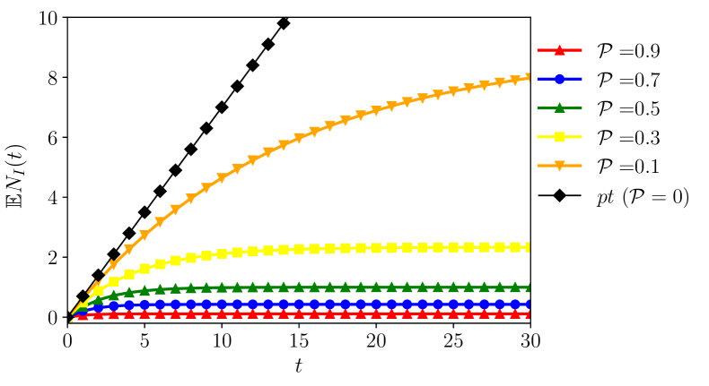
Figure 10: The plot shows $\mathbb{E}N_{I}(t)$ in (A.8) for different values of $\mathcal{P}$ given in the legend and fixed $p=0.7$. For small $t$ a linear behavior of order $\mathcal{Q}pt$ is observed, and for large $t$ the asymptotic value $\mathcal{Q}/\mathcal{P}$ is approached.

We are now interested in the expected number of DBP arrivals which, by (25) and (A.1), has the GF

$$\overline{\mathbb{E}{N}_{I}}(u)=\frac{\partial}{\partial v}\bar{\cal P}_{I}(v,u)\Big{|}_{v=1}=\frac{1}{1-u}\frac{{\bar{\psi}}_{I}(u)}{1-{\bar{\psi}}_{I}(u)}=\frac{\mathcal{Q}pu}{(1-u)[1-u(1-p\mathcal{P})]}$$ (A.7)

with $\bar{\cal P}_{I}(v,u)=\sum_{t=0}^{\infty}u^{t}\mathbb{E}v^{{N}_{I}(t)}$. We can invert this GF getting the formula

$$\mathbb{E}N_{I}(t)=\mathcal{Q}p\sum_{r=1}^{t}(1-p\mathcal{P})^{r-1}=\mathcal{Q}p\sum_{r=0}^{t-1}(1-p\mathcal{P})^{r}=\begin{cases}pt,&\mathcal{Q}=1,\\ \frac{\mathcal{Q}}{\mathcal{P}}\left(1-[1-p\mathcal{P}]^{t}\right),&\mathcal{Q}\in(0,1),\end{cases}$$ (A.8)

where, for $\mathcal{Q}\in(0,1)$, the number of arrivals approaches geometrically the finite asymptotic value $\mathbb{E}N_{I}(\infty)=\mathcal{Q}/\mathcal{P},$ which diverges in the type II limit $\mathcal{P}\to 0+$. We notice that in the type II limit $\mathcal{P}\to 0+$ the expected number of arrivals increases linearly in time as for the standard Bernoulli process. Namely,

$$\lim_{\mathcal{P}\to 0+}\mathbb{E}N_{I}(t)=\lim_{\mathcal{P}\to 0+}\frac{1}{\mathcal{P}}\left(1-[1-p\mathcal{P}t+O(\mathcal{P}^{2})]\right)=pt\,.$$ (A.9)

We show the behavior of $\mathbb{E}N_{I}(t)$ for some values of $\mathcal{P}$ in Fig. 10. We observe that the more defective is the process (i.e. the larger values of $\mathcal{P}$), the smaller is the average number of arrival events. The non-defective case ($\mathcal{P}=0$, in black in Fig. 10) is that of the standard binomial distribution (state probabilities of the non-defective standard Bernoulli process).

In Fig. 11 we show the state probabilities $\Phi^{(n)}(t)$ for the DBP evaluated at the specific time instant $t=6$ for several values of $\mathcal{P}$.

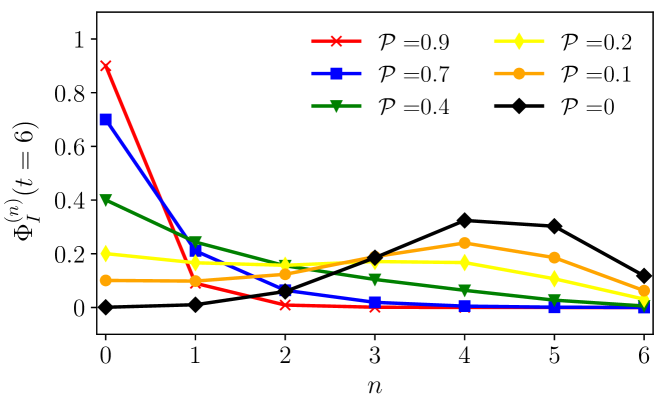
Figure 11: State probabilities of DBP (Equations (A.6) and (A.2)) at $t=6$ as a function of the number of arrivals $n$ for several values of $\mathcal{P}$ and fixed $p=0.7$. The standard binomial distribution of the non-defective case ${\cal P}=0$ is drawn in black color.

A.2 Defective Sibuya Process (DSP)

As a further prototypical example for a type I renewal process, we consider now the ‘defective Sibuya process’ (DSP) with waiting time GF

$${\bar{\psi}}_{I}(u)=\mathcal{Q}[1-(1-u)^{\mu}],\hskip 28.45274pt\mathcal{Q}\in(0,1],\,\mu\in(0,1).$$ (A.10)

The DSP waiting time density then is

$$\psi_{I}(t)=\mathcal{Q}(-1)^{t-1}\binom{\mu}{t},\hskip 28.45274ptt\in\mathbb{N},$$ (A.11)

We define the DSP as the renewal process with IID defective interarrival times which follow the PDF (A.11). The large-time asymptotics of (A.11) is

$$\psi_{I}(t)\sim\mathcal{Q}\frac{\mu}{\Gamma(1-\mu)}t^{-\mu-1},$$ (A.12)

and the DSP survival probability has the GF

$${\bar{\Phi}}^{(0)}_{I}(u)=\frac{1-{\bar{\psi}}_{I}(u)}{1-u}=\frac{\mathcal{P}}{1-u}+\mathcal{Q}(1-u)^{\mu-1}$$ (A.13)

where $\mathcal{P}=1-\mathcal{Q}$ can also be interpreted as the probability that no event has occurred in any finite time. Then, by conditioning, we can derive the state probabilities of the DSP as follows:

$$\Phi^{(n)}_{I}(t)=\mathbb{P}[N_{I}(t)=n]=\left(\Phi^{(0)}_{I}\star(\psi_{I}\star)^{n}\right)(t)=\frac{1}{t!}\frac{d^{t}}{du^{t}}\left({\bar{\Phi}}^{(0)}_{I}(u)[{\bar{\psi}}_{I}(u)]^{n}\right)\Big{|}_{u=0}.$$ (A.14)

In particular, we have for $n=0$,

$$\Phi_{I}^{(0)}(t)=\mathcal{P}+\mathcal{Q}(-1)^{t}\binom{\mu-1}{t},\qquad t\in\mathbb{N}_{0}.$$ (A.15)

We are now interested in the asymptotic expected number of events $\mathbb{E}{N}_{I}(t)$ of a DSP. For this purpose recall that

$$\mathbb{E}{N}_{I}(t)=\frac{\partial}{\partial v}{\cal P}_{I}(v,t)\big{|}_{v=1},$$ (A.16)

where ${\cal P}_{I}(v,t)=\mathbb{E}v^{{N}_{I}(t)}=\sum_{n=0}^{t}v^{n}\Phi_{I}^{(n)}(t)$. In order to get the large-time behavior, consider the GF of (A.16) that, using (A.14), reads

$$\begin{array}[]{clr}\displaystyle\overline{\mathbb{E}{N}_{I}}(u)&=\displaystyle\sum_{t=0}^{\infty}u^{t}\mathbb{E}{N}_{I}(t)\displaystyle={\bar{\Phi}}^{(0)}_{I}(u)\sum_{n=0}^{\infty}nv^{n-1}[{\bar{\psi}}_{I}(u)]^{n}\Big{|}_{v=1}&\\ \\ &=\displaystyle\frac{\partial}{\partial v}\frac{1-{\bar{\psi}}_{I}(u)}{1-u}\sum_{n=0}^{\infty}v^{n}[{\bar{\psi}}_{I}(u)]^{n}\Big{|}_{v=1}=\frac{\partial}{\partial v}\frac{1-{\bar{\psi}}_{I}(u)}{(1-u)[1-v{\bar{\psi}}_{I}(u)]}\Big{|}_{v=1}&\\ \\ &=\displaystyle\frac{{\bar{\psi}}_{I}(u)}{(1-u)[1-{\bar{\psi}}_{I}(u)]}=\frac{\mathcal{Q}[1-(1-u)^{\mu}]}{(1-u)[\mathcal{P}+\mathcal{Q}(1-u)^{\mu}]}&\end{array}$$ (A.17)

which can be further written as

$$\begin{array}[]{clr}\overline{\mathbb{E}{N}_{I}}(u)&=\displaystyle\frac{\mathcal{Q}}{\mathcal{P}(1-u)}\frac{1-(1-u)^{\mu}}{1+\frac{\mathcal{Q}}{\mathcal{P}}(1-u)^{\mu}}\\ \\ &=\displaystyle\frac{\mathcal{Q}}{\mathcal{P}(1-u)}\left(1-\frac{(1-u)^{\mu}}{\mathcal{P}[1+\frac{\mathcal{Q}}{\mathcal{P}}(1-u)^{\mu}]}\right)=\frac{\mathcal{Q}}{\mathcal{P}(1-u)}-\frac{\mathcal{Q}}{\mathcal{P}^{2}}{\bar{\cal E}}_{\mu}(u).&\end{array}$$ (A.18)

Remarkably, the first line of (A.18) contains the waiting time GF of the so-called fractional Bernoulli process of type A, first introduced and analyzed in [40] (see equation (75) in that paper):

$${\bar{\psi}}_{\text{fBa}}(u)=\frac{1-(1-u)^{\mu}}{1+\frac{\mathcal{Q}}{\mathcal{P}}(1-u)^{\mu}}.$$ (A.19)

Its inversion, the waiting time PDF $\psi_{\text{fBa}}(t)$ is a discrete approximation of the Mittag–Leffler distribution. In the second line of expression (A.18) the quantity

$${\bar{\cal E}}_{\mu}(u)=\frac{(1-u)^{\mu-1}}{1+\frac{\mathcal{Q}}{\mathcal{P}}(1-u)^{\mu}}$$ (A.20)

denotes the GF of ${\cal E}_{\mu}(t)$ which is a discrete approximation of the Mittag–Leffler function (see [33, 40] for explicit formulas). Then by invoking Tauberian arguments we can see that the limit $u\to 1-$ in the GF (A.20) yields the large time asymptotics of $\mathbb{E}N_{I}(t)$. Indeed, for large values of $t$, the expected number of events approaches a constant value with a power-law rate, namely

$$\begin{array}[]{clr}\displaystyle\mathbb{E}{N}_{I}(t)&=\displaystyle\frac{\mathcal{Q}}{\mathcal{P}}-\frac{\mathcal{Q}}{\mathcal{P}^{2}}{\cal E}_{\mu}(t)&\\ \\ &\sim\displaystyle\frac{\mathcal{Q}}{\mathcal{P}}-\frac{\mathcal{Q}}{\mathcal{P}^{2}}\frac{t^{-\mu}}{{\Gamma(1-\mu)}}&\\ \\ &\displaystyle\underset{t\to\infty}{\xrightarrow{\qquad}}\frac{\mathcal{Q}}{\mathcal{P}},&\end{array}$$ (A.21)

where we used that ${\cal E}_{\mu}(t)\sim\frac{t^{-\mu}}{\Gamma(1-\mu)}$ for $t\to\infty$ (as ${\bar{\cal E}}_{\mu}(u)\sim(1-u)^{\mu-1}$ for $u\to 1-$). One can see in (A.17) that for $\mathcal{Q}=1$ we have $\overline{\mathbb{E}{N}_{I}}(u)\sim(1-u)^{-\mu-1}$ as $u\to 1-$. This turns into the well-known diverging power-law behavior of the expected number of events of a type II Sibuya process, that is

$$\mathbb{E}N_{I}(t)\sim\frac{t^{\mu}}{\Gamma(1+\mu)}\underset{t\to\infty}{\xrightarrow{\qquad}}\infty.$$ (A.22)

A.3 General comments on defective renewal processes

The fact that $\mathbb{E}N_{I}(\infty)=\mathcal{Q}/\mathcal{P}$ (see (A.8) for the DBP and (A.21) for the DSP) holds in general for defective RPs. Indeed, consider a type I process with waiting time PDF $\psi_{I}(t)$ such that ${\bar{\psi}}_{I}(u)=\mathcal{Q}{\bar{\psi}}_{II}(u)$ where ${\psi}_{II}(t)$ is non-defective. Then, the expected number of arrivals of the type I RP has the GF

$$\overline{\mathbb{E}{N}_{I}}(u)=\frac{\mathcal{Q}}{\mathcal{P}(1-u)}\frac{\mathcal{P}{\bar{\psi}}_{II}(u)}{1-\mathcal{Q}{\bar{\psi}}_{II}(u)}=\frac{\mathcal{Q}}{(1-u)}\frac{{\bar{\psi}}_{II}(u)}{1-\mathcal{Q}{\bar{\psi}}_{II}(u)}$$ (A.23)

which, by Tauberian arguments, gives $\mathbb{E}{N}_{I}(\infty)=\mathcal{Q}/\mathcal{P}$. This result is corroborated by the following interpretation: at each renewal time a Bernoulli trial with success probability $\mathcal{P}$ is performed. If a success is obtained the related waiting time is infinitely long, otherwise it is sampled from $\psi_{II}$. Hence, in the limit $t\to\infty$ the random number of successes is geometric of parameter $\mathcal{P}$ regardless of the actual form of $\psi_{II}$. More formally. this can be inferred from (A.5) which holds true for any renewal process with defective PDF (76) such that ${\bar{\psi}}_{I}(u)\big{|}_{u=1}=\mathcal{Q}<1$. Therefore, we have the general result

$$\Phi_{I}^{(n)}(\infty)=(1-u)\Phi_{I}^{(0)}[{\bar{\psi}}_{I}(u)]^{n}\Big{|}_{u=1}=[1-{\bar{\psi}}_{I}(u)][{\bar{\psi}}_{I}(u)]^{n}\Big{|}_{u=1}=\mathcal{P}\mathcal{Q}^{n},\qquad n\in\mathbb{N}_{0}.$$ (A.24)

This means that, for $t\to\infty$ the state probabilities are a geometric distributed. From this relation, one immediately see the type I nature of the renewal processes $N_{I}(t)$ (see (14))

$$\Lambda=\lim_{n_{0}\to\infty}\mathbb{P}[N_{I}(\infty)>n_{0}]=\lim_{n_{0}\to\infty}\sum_{n=n_{0}+1}^{\infty}\Phi_{I}^{(n)}(\infty)=\lim_{n_{0}\to\infty}\mathcal{Q}^{n_{0}+1}=0.$$ (A.25)

Note that the process $N_{I}(t)$ and the process $M(t)$ considered in Section 3.1.2, represent different kinds of type I APs: $N_{I}(t)$ is a renewal process with IID defective interarrival times, whereas $M(t)$ is an externally stopped arrival process and, as we have already shown, it is not a renewal process. In the in which $M(t)$ has geometric non-defective absorbing time, the large time asymptotics of $M(t)$ is governed by an auxiliary renewal process ${\cal R}_{q}(t)$ which has defective IID interarrival times (see the GF (61) and the remarks thereafter).
Finally, we observe in (A.23) (when $\mathcal{Q}<1$) that the term $\frac{\mathcal{P}{\bar{\psi}}_{II}(u)}{1-\mathcal{Q}{\bar{\psi}}_{II}(u)}$ is the GF of the waiting time PDF of the time-changed type II RP ${\cal N}({N}_{II}(t))$ with a standard Bernoulli RP with success probability $\mathcal{P}$, and which is independent of $N_{II}$ (see e.g. [35]).

References

- [1] R. Aguech and W. Jedidi, New characterizations of completely monotone functions and Bernstein functions, a converse to Hausdorff’s moment characterization theorem. Arab Journal of Mathematical Sciences, 25(1), 57-82 (2019).
- [2] V.S. Barbu and N. Limnios, Semi-Markov Chains and Hidden Semi-Markov Models Toward Applications, Lecture Notes in Statistics, 191, Springer, New York (2008).
- [3] E. Barkai, Fractional Fokker-Planck equation, solution, and application, Phys. Rev. E 63, 046118 (2001).
- [4] E. Barkai, R. Flaquer-Galmés, V. Méndez, Ergodic properties of Brownian motion under stochastic resetting, Phys. Rev. E 108, 064102 (2023).
- [5] S. Bernstein, Sur les fonctions absolument monotones. Acta Mathematica, 52(1), 1–66, (1929).
- [6] A.A. Borovkov, Compound renewal processes. Cambridge University Press (2022).
- [7] D.O. Cahoy, F. Polito, Renewal processes based on generalized Mittag–Leffler waiting times, Commun Nonlinear Sci. Numer. Simul., Vol. 18 (3), 639-650 (2013).
- [8] C. Carey, The impacts of climate change on the annual cycles of birds, Phil. Trans. R. Soc. B 364, 3321–3330 (2009).
- [9] A.V. Chechkin, R. Metzler, J. Klafter, V. Yu. Gonchar, Introduction to the theory of Lévy flights, In: Anomalous Transport: Foundations and Applications, R. Klages, G. Radons, I.M. Sokolov (Editors), Wiley‐VCH Verlag (2008).
- [10] D.R. Cox, Renewal theory. Methuen & Co., Ltd., London; John Wiley & Sons, Inc., New York (1962).
- [11] I. Czarna, Z. Palmowski, P. Swiatek, Discrete time ruin probability with Parisian delay. Scandinavian Actuarial Journal, 2017(10), 854–869 (2017).
- [12] M. D’Ovidio, E. Orsingher and B. Toaldo, Time-changed processes governed by space-time fractional telegraph equations, Stoch. Anal. Appl., 32(6):1009–1045 (2014).
- [13] A. Di Crescenzo, A. Iuliano, V. Mustaro, G. Verasani, On the telegraph process driven by geometric counting process with Poisson-based resetting. Journal of Statistical Physics, 190(12), 191 (2023).
- [14] S. Eule, and J. J. Metzger, Non-equilibrium steady states of stochastic processes with intermittent resetting, New J. of Physics 18 033006 (2016).
- [15] W. Feller, On a generalization of Marcel Riesz’ potentials and the semi-groups generated by them. Comm. Sém. Mathém. Université de Lund, Tome suppl. dédié à M. Riesz, Lund, 73–81 (1952).
- [16] W. Feller, On semi-Markov processes. Proc. Natl. Acad. Sci. USA 51, 653-9 (1964).
- [17] C. Godrèche and J. M. Luck, Statistics of the Occupation Time of Renewal Processes, J. Stat. Phys. 104, 489 (2001).
- [18] C. Godrèche, and J.M. Luck, Replicating a renewal process at random times, Journal of Statistical Physics, 191(1), 4 (2023).
- [19] R. Gorenflo, F. Mainardi, Continuous time random walk, Mittag-Leffler waiting time and fractional diffusion: Mathematical aspects. In: R. Klages, G. Radons, I.M. Sokolov, editors. Anomalous transport: Foundations and applications. Weinheim, Germany: Wiley-VCH; (2008).
- [20] P.R. Grant, B.R. Grant, R.B. Huey, M.T.J. Johnson, A.H. Knoll, J. Schmitt, Evolution caused by extreme events, Evolution caused by extreme events. Phil. Trans. R. Soc. B 372: 20160146 (2017).
- [21] G. Grimmett. Probability on graphs: random processes on graphs and lattices. Cambridge University Press (2018).
- [22] G. Kersting, C. Minuesa, Defective Galton-Watson processes in varying environment. Bernoulli, 28(2), 1408-1431, (2022).
- [23] R. Kutner, J. Masoliver, The continuous time random walk, still trendy: Fifty-year history, state of art and outlook. Eur. Phys. J. B 90:50 (2017).
- [24] N. Laskin, Fractional Poisson process. Commun. Nonlinear Sci. Numer. Simul. 8, 3-4, 201-213 (2003).
- [25] G. Latouche, M.-A. Remiche, P. Taylor, Transient Markov Arrival Processes, The Annals of Applied Probability, Vol. 13, No. 2, 628–640 (2003).
- [26] P. Lévy, Processus semi-Markovien. Proc Int. Congr. Math. 3, 416–26 (1956).
- [27] N. Limnios, A. Swishchuk, Discrete-Time Semi-Markov Random Evolutions and Their Applications, Springer (2023).
- [28] F. Mainardi, Lévy Stable Distributions in the Theory of Probability, Lecture Notes on Mathematical Physics (2007).
- [29] M.M. Meerschaert, A. Sikorski, Stochastic models for fractional calculus. De Gruyter studies in mathematics, vol. 43, Berlin-Boston: Walter de Gruyter (2019).
- [30] M.M. Meerschaert and P. Straka. Semi-Markov approach to continuous time random walk limit processes. Ann. Probab. 42(4):1699–1723 (2014).
- [31] R. Metzler, J. Klafter, The random walk’s guide to anomalous diffusion : A fractional dynamics approach, Phys. Rep. 339, 1–77 (2000).
- [32] T.M. Michelitsch, A.P. Riascos, Generalized fractional Poisson process and related stochastic dynamics. Fract. Calc. Appl. Anal., Vol. 23, 3:656–693 (2020).
- [33] T.M. Michelitsch, F. Polito, A.P. Riascos, On discrete time Prabhakar-generalized fractional Poisson processes and related stochastic dynamics, Physica A 565, 125541 (2021).
- [34] T.M. Michelitsch, F. Polito, A.P. Riascos, Biased Continuous-Time Random Walks with Mittag–Leffler Jumps, Fractal Fract. 4, (4), 51, (2020).
- [35] T.M. Michelitsch, F. Polito, A.P. Riascos, Asymmetric random walks with bias generated by discrete-time counting processes, Commun. Nonlinear. Sci. Numer. Simul. 109, 106121 (2022).
- [36] T.M. Michelitsch, F. Polito, A.P. Riascos, Squirrels can remember little: A random walk with jump reversals induced by a discrete-time renewal process, Commun. Nonlinear. Sci. Numer. Simul. 118, 107031 (2023).
- [37] T.M. Michelitsch, F. Polito, A.P. Riascos, Semi-Markovian Discrete-Time Telegraph Process with Generalized Sibuya Waiting Times, Mathematics, 11, 471 (2023).
- [38] T.M. Michelitsch, A.P. Riascos, B.A. Collet, A. Nowakowski, F. Nicolleau, Fractional Dynamics on Networks and Lattices, ISTE-Wiley, London, (2019).
- [39] E.W. Montroll, G.H. Weiss, Random walks on lattices II, J. Math Phys. 6(2):167–81 (1965).
- [40] A. Pachon, F. Polito, C. Ricciuti, On discrete-time semi-Markov processes, Discrete and Continuous Dynamical Systems Series B 26, 3, 1499-1529 (2021).
- [41] K.A. Penson and K. Górska, Exact and Explicit Probability Densities for One-Sided Lévy Stable Distributions, Phys. Rev. Lett. 105, 210604 (2010).
- [42] G. Pólya, Über eine Aufgabe der Wahrscheinlichkeitsrechnung betreffend die Irrfahrt im Straßennetz, Math. Ann. 84, 149-160 (1921).
- [43] A.P. Riascos, T.M. Michelitsch, and A. Pizarro-Medina, Nonlocal biased random walks and fractional transport on directed networks, Phys. Rev. E 102, 022142 (2020).
- [44] A.P. Riascos, F.H. Padilla, A measure of dissimilarity between diffusive processes on networks, J. Phys. A: Math. Theor. 56 145001 (2023).
- [45] R.L. Schilling, R. Song, Z. Vondraček. Bernstein Functions: Theory and Applications, 2nd ed.; De Gruyter Studies in Mathematics, 37; Walter de Gruyter & Co.: Berlin, Germany, (2012).
- [46] R.K. Singh, K. Górska, T. Sandev, General approach to stochastic resetting. Phys Rev E 105:064133 (2022).
- [47] P. Van Mieghem, Graph Spectra for Complex Networks (New York: Cambridge University Press (2011).
- [48] W. Wang, E. Barkai, Fractional advection diffusion asymmetry equation, derivation, solution and application, J. Phys. A: Math. Theor. 57 035203 (2024).
- [49] D.V. Widder, The Laplace Transform; Princeton University Press: Princeton, NJ, USA, (1941).
- [50] S. Zacks, D. Perry, D. Bshouty, S. Barlev, Distributions of stopping times for compound Poisson processes with positive jumps and linear boundaries, Communications in Statistics. Stochastic Models, 15:1, 89-101 (1999).