User Tracking and Direction Estimation Codebook Design for IRS-Assisted mmWave Communication

Abstract

Future communication systems are envisioned to employ intelligent reflecting surfaces (IRSs) and the millimeter wave (mmWave) frequency band to provide reliable high-rate services. For mobile users, the time-varying channel state information (CSI) requires adequate adjustment of the reflection pattern of the IRS. We propose a novel codebook-based user tracking (UT) algorithm for IRS-assisted mmWave communication, allowing suitable reconfiguration of the IRS unit cell phase shifts, resulting in a high reflection gain. The presented algorithm acquires the direction information of the user based on a peak likelihood-based direction estimation. Using the direction information, the user’s trajectory is extrapolated to proactively update the adopted codeword and adjust the IRS phase shift configuration accordingly. Furthermore, we conduct a theoretical analysis of the direction estimation error and utilize the obtained insights to design a codebook specifically optimized for direction estimation. Our numerical results reveal a lower direction estimation error of the proposed UT algorithm when employing our designed codebook compared to codebooks from the literature. Furthermore, the average achieved signal-to-noise ratio (SNR) as well as the average effective rate of the proposed UT algorithm are analyzed. The proposed UT algorithm requires only a low overhead for direction and channel estimation and avoids outdated IRS phase shifts. Furthermore, it is shown to outperform two benchmark schemes based on direct phase shift optimization and hierarchical codebook search, respectively, via computer simulations.

I Introduction

The continuous development of new communication systems, such as the sixth-generation wireless communication standard (6G), aims to provide higher data rates to accommodate the steadily increasing user demands. To meet these requirements, previously unused spectrum, such as the millimeter wave (mmWave) band (30 GHz - 300 GHz), is considered of great interest [2]. However, for mmWave communication systems, the line-of-sight (LoS) path is usually significantly stronger than the remaining multi-path components [2]. Therefore, obstruction of the LoS causes severe performance degradation in these systems. To mitigate this effect, intelligent reflecting surfaces (IRSs) have been introduced. These are passive devices consisting of many small programmable unit cells that reflect electromagnetic waves in a controllable manner [3, 4]. By placing IRSs strategically, the coverage of a base station (BS) can be extended to otherwise obstructed areas, by providing a virtual LoS from the BS to a user via the IRS [3, 4].

When an IRS is utilized to enable communication between a BS and a mobile user, the phase shifts of the IRS unit cells need to be updated regularly according to the user’s current position. This task can be facilitated by user tracking (UT) techniques that update the BS’s estimate of the real-time direction of the user relative to the IRS. In particular, once the direction of the user (or an estimate of it) is available to the BS, the IRS phase shifts can be configured efficiently via codebook-based IRS configuration [5]. Compared to configuring the phase shifts of the IRS unit cells individually [6, 7], which requires full channel state information (CSI) knowledge, it suffices for codebook-based IRS configuration to know the direction of the user in order to select the optimal codeword, i.e., the codeword whose beam pattern overlaps most with the actual direction of the user. Hence, accurate UT in IRS-assisted systems enables the efficient configuration of IRS unit cells for data transmission.

However, acquiring information about the user’s position is itself a difficult problem in IRS-assisted systems. For systems without IRSs, direction estimation has been studied extensively and powerful digital signal processing algorithms, such as the multiple signal classification (MUSIC) algorithm [8] and several variants of it (see [9] for a recent review of algorithms for direction estimation) have been proposed. However, those algorithms require the continuous measurement of the received signal at an antenna array. Hence, since standard (passive) IRSs cannot perform sensing and processing, these algorithms are not applicable in IRS-assisted settings. Alternatively, neural network based prediction approaches can be employed for specific scenarios where movement data is available to training the neural network, see, e.g., [10, 11]. However, the requirement for training data limits the applicability of such models, especially when user movement patterns change over time.

It was also proposed in the literature to track the user’s direction using model-based statistical signal processing tools, such as the Kalman filter [12] or the extended Kalman filter [13], or linear extrapolation [14]. However, the accuracy of these methods depends on the availability of models that map the measurements to the user’s direction parameters [12, 13] or the strong assumption of linear user trajectories [14]. However, for the general case of mobile users that move nonlinearly, i.e., the user’s direction is a nonlinear function of time, a mapping from the measurement, i.e., the received signal at either the BS or the user, to the user’s direction relative to the IRS is not known to date. Hence, these model-based user tracking methods are not applicable to IRS-assisted systems.

For IRS-assisted systems, an algorithm for estimating the user’s direction relative to the IRS based on minimizing the Cramer-Rao bound (CRB) of the direction estimation error has been proposed in [15]. However, this algorithm requires full CSI knowledge, which is difficult to obtain for IRS-assisted systems in practice. Furthermore, the scheme proposed in [15] requires adjusting the phase shifts of all IRS elements individually, which is computationally challenging for large IRSs and may be infeasible in real-time. Finally, the authors of [16] propose a UT algorithm for a roadside setting where several IRSs are used to maintain LoS connections to cars moving along the road. However, the movement trajectories of the cars in [16] are assumed to be linear and, hence, the proposed scheme does not apply in general, when nonlinear movement of user devices is considered. To the best of the authors’ knowledge, a UT algorithm for general user movement scenarios which is applicable when full CSI, i.e., knowledge of all multi-path components, is not available has not been proposed for IRS-assisted systems, so far.

In this paper, we propose a novel scheme for user direction estimation and tracking in IRS-assisted systems to overcome the shortcomings of existing schemes. On the one hand, the UT scheme proposed in this paper is codebook-based and, hence, features efficient IRS configuration supporting real-time use cases. While existing codebooks are either of fixed size [17], i.e., of limited flexibility, or optimized for data transmission, i.e., to achieve the highest possible reflection gains, [5, 18, 19, 20], the direction estimation codebook proposed in this paper is of variable size and designed specifically for direction estimation. On the other hand, the proposed tracking scheme does not depend on the assumption of linear user trajectories, but is applicable to general nonlinear user movement. The proposed algorithm repeatedly estimates the user direction in regular time intervals using a peak likelihood-based approach facilitated by the proposed direction estimation codebook. Then, based on these direction estimates, the user’s trajectory is extrapolated in the subsequent time blocks and the corresponding optimal codewords for data transmission are selected from a second codebook, the data transmission codebook. In order to design the direction estimation codebook, first a theoretical analysis of the expected estimation error using a first-order approximation of the IRS response function is performed. Then, based on the error analysis, a gradient descent algorithm for finding a locally optimal beam shape is derived.

The main contributions can be summarized as follows:

• We propose a novel beam pattern design specifically optimized for minimizing the user direction estimation error in the considered IRS-assisted system. The direction estimation codebook derived from the proposed beam pattern is practically realizable since it implicitly accounts for beam shape limitations imposed by the codebook-based IRS configuration.

• We introduce a codebook-based UT algorithm that first estimates the direction based on the proposed direction estimation codebook and then extrapolates the current user direction. The extrapolated direction is used to proactively determine when the IRS codeword for data transmission has to be changed and to optimally select the new codeword.

• We provide a comprehensive analysis of the overall performance and overhead that the proposed communication scheme achieves.

The simulation results confirm that the proposed UT algorithm can maintain the LoS connection to a mobile user, even for general nonlinear movement patterns. They also reveal that the direction estimation error is significantly lower when employing the proposed direction estimation codebook, compared to two reference codebooks from the literature optimized for data transmission. Furthermore, the proposed UT algorithm achieves a significantly higher effective rate compared to two baseline schemes, which are based on the perfect CSI of the IRS-to-user channel and codebook-based IRS configuration for data transmission via hierarchical search, respectively.

In the conference version of this paper [1], we introduced a preliminary version of the UT algorithm presented in this paper. However, the codebook used for direction estimation in [1] was not optimized for direction estimation and a comprehensive performance analysis of the proposed scheme was not provided in [1]. Hence, this paper significantly extends [1] towards a mature UT scheme for IRS-assisted mmWave systems.

The remainder of this paper is organized as follows. In Section II, we introduce the considered system model. The UT algorithm and the codebook design are presented in Sections III and IV, respectively. Finally, Sections V and VI report our numerical results and conclusions, respectively.

Notations: Lower case and upper case bold letters denote vectors and matrices, respectively. The transpose and conjugate transpose of matrix $\mathbf{A}$ are denoted by $\mathbf{A}^{\mathrm{T}}$ and $\mathbf{A}^{\mathrm{H}}$, respectively. The $i$-th element of vector $\mathbf{a}$ is denoted by $[\mathbf{a}]_{i}$, and the element in the $i$-th row and $j$-th column of matrix $\mathbf{A}$ is denoted by $[\mathbf{A}]_{i,j}$. The distribution of a circularly symmetric complex Gaussian random vector with mean vector $\mathbf{x}$ and covariance matrix $\mathbf{A}$ is represented by $\mathcal{CN}(\mathbf{x},\mathbf{A})$ and the imaginary unit is denoted by $\mathrm{j}=\sqrt{-1}$. The all-zero vector of length $n$, the all-one vector of length $n$, and the identity matrix of size $n\times n$ are denoted as $\mathbf{0}_{n}$, $\mathbf{1}_{n}$, and $\mathbf{I}_{n}$, respectively. The complex conjugate, absolute, and expected values of a scalar $x$ are denoted by $x^{*}$, $|x|$, and $\mathcal{E}\{x\}$, respectively. The main diagonal vector and the rank of a matrix $\mathbf{X}$ are denoted as $\mathrm{Diag}(\mathbf{X})$ and $\mathrm{Rank}(\mathbf{X})$, respectively. The Hadamard (element-wise) and Kronecker products are denoted by $\odot$ and $\otimes$, respectively. The cardinality of set $\mathcal{M}$ is denoted by $|\mathcal{M}|$. $\mathbb{N}$, $\mathbb{R}$, $\mathbb{R}_{+}$, and $\mathbb{C}$ denote the sets of natural, real, positive real, and complex numbers, respectively. For any real number $x$, $\lfloor x\rfloor$ denotes the floor of $x$. Finally, the big-O notation is denoted by $\mathcal{O}(\cdot)$.

II System Model

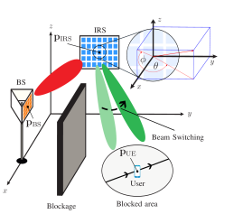
Figure 1: The considered system consists of a BS, an IRS, and a user that moves within an obstructed area. The direct link between the BS and the user is blocked.

We consider the IRS-assisted mmWave communication system illustrated in Fig. 1. In this system, a BS transmits data to a mobile user who is located in an area to which no LoS path from the BS is available throughout the considered time frame. The BS and the user device are equipped with uniform planar arrays (UPAs) comprising $Q_{\mathrm{BS}}=Q_{\mathrm{BS},1}\times Q_{\mathrm{BS},2}$ and $Q_{\mathrm{UE}}=Q_{\mathrm{UE},1}\times Q_{\mathrm{UE},2}$ elements with spacing $d_{\mathrm{BS}}$ and $d_{\mathrm{UE}}$, respectively, and both employ analog beamforming. We equip the considered communication environment with a Cartesian coordinate system, cf. Fig. 1, such that the BS UPA lies in the $x$-$z$ plane and the BS and user UPAs are centered at Cartesian coordinates $\mathbf{p}_{\mathrm{BS}}\in\mathbb{R}^{3}$ and $\mathbf{p}_{\mathrm{UE}}(t)\in\mathbb{R}^{3}$, respectively. Both $\mathbf{p}_{\mathrm{UE}}(t)$ and the orientation of the user UPA change as functions of time $t$ and are not known to the BS.

The situation illustrated in Fig. 1 in which no LoS between BS and user is available commonly arises in mmWave systems due to the pronounced attenuation of high-frequency signals. To mitigate this lack of a direct signal propagation path, a passive IRS to which a LoS link from the BS is available is employed to assist the communication. The IRS comprises $Q_{\mathrm{IRS}}=Q_{\mathrm{IRS},1}\times Q_{\mathrm{IRS},2}$ unit cells of sizes $A_{\mathrm{UC}}=d_{\mathrm{IRS}}^{2}$ and is centered at $\mathbf{p}_{\mathrm{IRS}}=[x_{\mathrm{IRS}},y_{\mathrm{IRS}},z_{\mathrm{IRS}}]^{\mathrm{T}}\in\mathbb{R}^{3}$. For simplicity of presentation and without loss of generality, in this paper, we assume that the IRS is square, i.e., $Q_{\mathrm{IRS},1}=Q_{\mathrm{IRS},2}=Q$, and lies in the $y$-$z$ plane, i.e., orthogonal to the BS UPA .

In principle, the direction of the user relative to the IRS at time $t$ can be described in terms of the azimuth and elevation angles of $\mathbf{p}_{\mathrm{UE}}(t)$. However, for the problems of estimating and tracking the direction of the user studied in this paper, it is beneficial instead to consider the direction of $\mathbf{p}_{\mathrm{UE}}(t)$ relative to the line $\mathbf{p}_{\mathrm{IRS}}+a[1,0,0]^{\mathrm{T}}$, $a\in\mathbb{R}_{+}$, i.e., the normal direction of the IRS. To this end, we introduce the notation $[\theta,\phi]^{\mathrm{T}}$, where $\theta$ and $\phi$ for any $[x,y,z]\in\mathbb{R}_{+}\times\mathbb{R}^{2}$ are defined as $\theta=\arctan\left(\frac{y-y_{\mathrm{IRS}}}{x}\right)$ and $\phi=\arctan\left(\frac{z-z_{\mathrm{IRS}}}{x}\right)$. Furthermore, whenever it is necessary to consider the azimuth and elevation angles in the following, we use the classical definition, where the elevation angle $\epsilon$ is the angle between the direction vector and the normal vector of the respective array, and the azimuth angle $\alpha$ is the angle between the horizontal and vertical axis of the direction vector projection onto the array plane.

II-A Time Block Structure

BS, IRS, and user communicate in the considered system in transmission blocks (TBs) of fixed length $T$. Hereby, the TBs are enumerated by $k\in\mathbb{N}_{0}$ and the starting time of each TB $k\in\mathbb{N}_{0}$ is denoted as $t_{k}=kT$. The TB structure proposed in this paper, which is identical for all TBs, is shown in Fig. 2. In the first sub-block of length $T_{\mathrm{UC}}$ of each TB $k$, the so-called user configuration (UC) sub-block, the user’s beamformer is updated. Regularly updating the user’s beamformer is necessary to account for the time-varying user position and user UPA orientation. However, since the number of antennas of the user device is typically small in practical systems, the user UPA’s beams are rather wide and, consequently, a single update of the user’s beamformer per TB is considered sufficient. The second sub-block of length $T_{\mathrm{IDE}}$ of each TB, called IRS direction estimation (IDE) sub-block, is used for estimating the direction of the user relative to the IRS. In the IDE sub-block, the BS repeatedly sends a pilot sequence, while the IRS cycles through different IRS beam patterns, i.e., codewords. Based on the received signals for the different IRS configurations, the user performs the direction estimation (and feeds the estimated direction back to the BS). The remaining part of each TB consist of $\eta\in\mathbb{N}$ pairs of channel estimation (CE) sub-blocks and data transmission (DT) sub-blocks, where each CE and DT sub-block is of length $T_{\mathrm{CE}}$ and $T_{\mathrm{DT}}$, respectively. Since the end-to-end communication channel between BS and user is affected by small-scale fading, the end-to-end CSI is estimated in the CE sub-blocks on the timescale of the channel coherence time $T_{\mathrm{coh}}$ to facilitate data detection in the DT blocks. We note that since in the considered system a LoS is always available from the BS to the IRS, the BS’s beam can be statically aligned with the LoS direction towards the IRS. Since no reconfiguration is needed during the system’s operation, no time resources need to be allocated in the TB structure for configuring the BS.

Considering the proposed TB structure, two different time scales are employed for CE on the one hand and UC and IDE on the other hand. Specifically, similar to [21], CE is carried out frequently, while UC and IDE are performed comparatively infrequently . The duration of one TB is $T=T_{\mathrm{UC}}+T_{\mathrm{IDE}}+\eta(T_{\mathrm{CE}}+T_{\mathrm{DT}})$. To ensure that the end-to-end channel is quasi static during UC, CE, and DT, the IRS configuration can only be changed directly before each UC sub-block at times $t=t_{k}$ and directly before each CE sub-block at times $t_{k,\kappa}=t_{k}+T_{\mathrm{UC}}+T_{\mathrm{IDE}}+\kappa(T_{\mathrm{CE}}+T_{\mathrm{DT}})$, $\kappa=0,...,\eta-1$, but not within any UC, CE, or DT sub-block. Furthermore, the IRS phase shift configurations are drawn from the direction estimation codebook $\mathcal{M}_{\mathrm{IDE}}$ for the IDE sub-blocks and from the data transmission codebook $\mathcal{M}_{\mathrm{DT}}$ for all other sub-blocks. For simplicity, we assume that the IRS can be reconfigured instantly without any delay.

II-B User Tracking

Since the IRS typically comprises many unit cells, it can create narrow reflection beams, e.g., as compared to the user’s UPA beams. Consequently, the received power at the user is very low when the IRS beam is not aligned with the user direction. Hence, the IRS beam pattern needs to be updated even when the direction of the user changes only slightly and, to this end, it is beneficial if the BS keeps track of the user’s current position.

In the user tracking scheme proposed in this paper the IRS beam is adapted to changes in the user’s direction even within one TB in order to avoid huge drops in the received signal power due to beam misalignment between two consecutive IDE blocks. To this end, the BS extrapolates the user’s current direction at each $t_{k,\kappa}$, $\kappa=1,\ldots,\eta-1$, based on the direction estimates obtained in the IDE sub-blocks of previous TBs $k^{\prime}<k$. In this way, the IRS phase shifts are reconfigured frequently and changes in the user’s position are accounted for within the same TB.

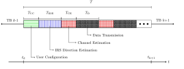
Figure 2: Transmission block in the proposed block structure.

II-C Signal Model

The downlink signal received at the user from the BS at any time $t$ is given by [5]

$$r(\mathbf{m},t)=\mathbf{f}_{\mathrm{UE}}^{\mathrm{H}}[k]\Big{(}\mathbf{H}_{\mathrm{r}}\mathbf{\Omega}(\mathbf{m})\mathbf{H}_{\mathrm{t}}\mathbf{f}_{\mathrm{BS}}s(t)+\mathbf{n}(t)\Big{)},$$ (1)

where $\mathbf{f}_{\mathrm{UE}}[k]\in\mathbb{C}^{Q_{\mathrm{UE}}}$, $\mathbf{f}_{\mathrm{BS}}\in\mathbb{C}^{Q_{\mathrm{BS}}}$, $s(t)$, and $\mathbf{n}(t)\sim\mathcal{CN}(\mathbf{0}_{Q_{\mathrm{UE}}},\sigma^{2}\mathbf{I}_{Q_{\mathrm{UE}}})$ denote the beamforming vector at the user in TB $k=\lfloor t/T\rfloor$, the beamforming vector at the BS, the BS transmit signal, and the additive white Gaussian noise (AWGN) at the user, respectively. Furthermore, $\mathbf{H}_{\mathrm{r}}\in\mathbb{C}^{Q_{\mathrm{UE}}\times Q_{\mathrm{IRS}}}$ and $\mathbf{H}_{\mathrm{t}}\in\mathbb{C}^{Q_{\mathrm{IRS}}\times Q_{\mathrm{BS}}}$ represent the IRS-to-user and the BS-to-IRS channels, respectively. Moreover, we define the end-to-end channel as $h_{\mathrm{e2e}}=\mathbf{f}_{\mathrm{UE}}^{\mathrm{H}}[k]\mathbf{H}_{\mathrm{r}}\mathbf{\Omega}(\mathbf{m})\mathbf{H}_{\mathrm{t}}\mathbf{f}_{\mathrm{BS}}$, where diagonal matrix $\mathbf{\Omega}(\mathbf{m})$ contains the reflection coefficients of all IRS unit cells for codeword $\mathbf{m}$ and $\bm{\mathrm{m}}$ is drawn from either $\mathcal{M}_{\mathrm{DT}}$ or $\mathcal{M}_{\mathrm{IDE}}$. For notational convenience, we further define $\bm{\omega}(\mathbf{m})=\mathrm{Diag}(\mathbf{\Omega}(\mathbf{m}))$.

The beamformer at the BS, $\mathbf{f}_{\mathrm{BS}}$, is set to align with the (static) LoS direction from the BS to the IRS. For the beamformer at the user, $\mathbf{f}_{\mathrm{UE}}[k]$, we assume that it is obtained from a DFT codebook having a size equal to the number of user antennas $Q_{\mathrm{UE}}$. Specifically, in each UC block, the BS repeatedly sends a pilot sequence while the user cycles through all candidate codewords from the DFT codebook. During the testing of all candidate codewords for UC, the IRS unit cell phase shifts are fixed to one single codeword. Finally, $\mathbf{f}_{\mathrm{UE}}[k]$ is selected as the codeword that resulted in the highest received power. For a pilot sequence of $N_{\mathrm{UC}}$ symbols, each of length $T_{\mathrm{S}}$, the duration of the UC sub-block is $T_{\mathrm{UC}}=Q_{\mathrm{UE}}N_{\mathrm{UC}}T_{\mathrm{S}}$.

II-D Channel Model

The channels considered in this paper comprise only a few multi-path components, due to the high path loss at mmWave frequencies. Furthermore, since the BS-to-IRS and IRS-to-user channels are assumed to be unobstructed, the respective LoS paths are dominant. To account for additional multi-path components, we assume that there are $L_{\mathrm{t}}$ and $L_{\mathrm{r}}$ scatterers at fixed positions in the BS-to-IRS and IRS-to-user channels, respectively. Consequently, the channels can be characterized according to a geometric channel model, where the channel matrices follow a Rician distribution, see also [23].

The BS-to-IRS and IRS-to-user channel matrices are constructed as $\mathbf{H}_{\mathrm{t}}=\mathbf{A}_{\mathrm{t}}\mathbf{\Sigma}_{\mathrm{t}}\mathbf{A}_{\mathrm{BS}}^{\mathrm{H}}$ and $\mathbf{H}_{\mathrm{r}}=\mathbf{A}_{\mathrm{UE}}\mathbf{\Sigma}_{\mathrm{r}}\mathbf{A}_{\mathrm{r}}^{\mathrm{H}}$, respectively [5]. Here, steering matrices $\mathbf{A}_{i}=[\mathbf{a}(\bm{\psi}_{i,1}),...,\mathbf{a}(\bm{\psi}_{i,L_{i}+1})]$, $i\in\{\mathrm{UE},\mathrm{t},\mathrm{r},\mathrm{BS}\}$, contain the steering vectors $\mathbf{a}(\bm{\psi}_{i,l})$ for angle-of-arrival ($i=t,\mathrm{UE}$) or angle-of-departure ($i=\mathrm{BS},r$) $\bm{\psi}_{i,l},l\in\{1,...,L_{i}+1\}$ of propagation path $(i,l)$ and diagonal matrices $\mathbf{\Sigma}_{i},i\in\{\mathrm{t},\mathrm{r}\}$, contain the path gains associated with channel $i$.

For any device $I\in\{\mathrm{BS},\mathrm{IRS},\mathrm{UE}\}$, every direction relative to $I$ is defined as $\bm{\mathrm{\psi}}_{I}=[\alpha_{I},\epsilon_{I}]$, where $\alpha_{I}$ and $\epsilon_{I}$ denote the corresponding azimuth and elevation angle, respectively. The steering vector for $\bm{\mathrm{\psi}}_{I}$ is then given by [18]

$$\mathbf{a}(\bm{\mathrm{\psi}}_{I})=\mathbf{a}_{1}(\bm{\mathrm{\psi}}_{I})\otimes\mathbf{a}_{2}(\bm{\mathrm{\psi}}_{I}),$$ (2)

where $[\mathbf{a}_{\mu}(\bm{\mathrm{\psi}}_{I})]_{q}=\mathrm{e}^{\mathrm{j}\frac{2\pi d_{I}}{\lambda}A_{\mu}(\bm{\mathrm{\psi}}_{I})\times\left(-\frac{Q_{I,\mu}-1}{2}+(q-1)\right)}$, for $q\in\{1,...,Q_{I,\mu}\}$, $\mu\in\{1,2\}$, where $\lambda$ denotes the wavelength and $A_{1}(\bm{\mathrm{\psi}}_{I})$ $=$ $\sin(\epsilon_{I})\cos(\alpha_{I})$ and $A_{2}(\bm{\mathrm{\psi}}_{I})$ $=$ $\sin(\epsilon_{I})\sin(\alpha_{I})$ define the phase differences between adjacent array elements in horizontal and vertical direction, respectively. For convenience, and in slight abuse of notation, we use the notations $\mathbf{a}(\bm{\mathrm{\psi}}_{\mathrm{IRS}})$ and $\mathbf{a}(\bm{\mathrm{\psi}})$ interchangeably, where $\bm{\mathrm{\psi}}=[\theta,\phi]$ is given in the $\theta$, $\phi$ coordinates defined above and $[\alpha_{\mathrm{IRS}},\epsilon_{\mathrm{IRS}}]$ is mapped to $[\theta,\phi]$ as $\alpha_{\mathrm{IRS}}=\arctan\left(\sqrt{\tan^{2}(\theta)+\tan^{2}(\phi)}\right)$ and $\epsilon_{\mathrm{IRS}}=\arctan\left(\frac{\tan(\theta)}{\tan(\phi)}\right)+\frac{\pi}{2}\left(1-\mathrm{sign}\left(\tan(\phi)\right)\right)$. The attenuation of the electromagnetic waves along any propagation path is modeled here as free space path loss, i.e.,

$$[\mathbf{\Sigma}_{i}]_{l,l}=\left(\upsilon_{i,l}\frac{\lambda}{4\pi\delta_{i,l}}\right)^{2},\;i\in\{\mathrm{t},\mathrm{r}\},$$ (3)

where $\upsilon_{i,l}$ and $\delta_{i,l},l\in\{1,...,L_{i}+1\}$ denote the reflection coefficient and the distance that the electromagnetic waves travel along path $(i,l)$, respectively. Assigning, without loss of generality, index $1$ to the LoS directions, e.g., $\bm{\psi}_{\mathrm{BS},1}$ corresponds to the LoS direction from the BS to the IRS, the ratio of the gain of the LoS path to the cumulative gain of all other paths is denoted by

$$K_{i}=\frac{[\mathbf{\Sigma}_{i}]_{1,1}}{\sum_{l=2}^{L_{i}+1}[\mathbf{\Sigma}_{i}]_{l,l}},\;\;i\in\{\mathrm{t},\mathrm{r}\}.$$ (4)

II-E Codebook Model

We recall from above that $\mathcal{M}_{\mathrm{IDE}}$ denotes the codebook used to configure the phase shifts of the IRS unit cells in the IDE sub-blocks and assume, similar to [18, 24], that the phase shift vectors for the horizontal and vertical directions are adjusted separately. Even though the full flexibility of the IRS is not available under this assumption, it is critical in order to reduce the computational complexity of the beam design. Specifically, only $2Q$ phase shifts need to be optimized as compared to $Q^{2}$ phase shifts when optimizing the phase shift of each unit cell individually. Consequently, the phase shift vector corresponding to codeword $\bm{\mathrm{m}}\in\mathcal{M}_{\mathrm{IDE}}$, $\bm{\mathrm{\omega}}(\bm{\mathrm{m}})$, factorizes into a horizontal and a vertical component as follows

$$\bm{\omega}(\mathbf{m})=\bm{\omega}_{1}(m_{1})\otimes\bm{\omega}_{2}(m_{2}),$$ (5)

where $\bm{\omega}_{1}(m_{1}),\bm{\omega}_{2}(m_{2})\in\mathbb{C}^{Q}$ denote the IRS phase shift vectors in the horizontal and vertical directions, respectively, and we can write $\mathbf{m}=[m_{1},m_{2}]^{T}$, where $m_{1},m_{2}\in\{0,...,M-1\}$ and $M$ denotes the codebook size in both horizontal and vertical direction. According to this codebook construction, $\mathcal{M}_{\mathrm{IDE}}$ comprises $|\mathcal{M}_{\mathrm{IDE}}|=M^{2}$ codewords.

To further simplify the codebook design and facilitate real-time applications, in this paper, we employ the same beam shape $\bm{\omega}_{\mathcal{M}}\in\mathbb{C}^{Q}$ for each codeword, such that the presented codebook design problem, cf. Section IV, has to be solved only once per codebook and not for each codeword individually. Consequently, we have

$$\begin{split}&\bm{\omega}_{\mu}(m_{\mu})=\bm{\mathrm{\omega}}_{\mathcal{M}}\odot\bm{\mathrm{\omega}}_{m_{\mu}}\\ &\;\;=\bm{\omega}_{\mathcal{M}}\odot\left[\mathrm{e}^{\mathrm{j}\left(\frac{4\pi d_{\mathrm{IRS}}m_{\mu}}{\lambda M}-\pi\right)1},...,\mathrm{e}^{\mathrm{j}\left(\frac{4\pi d_{\mathrm{IRS}}m_{\mu}}{\lambda M}-\pi\right)Q}\right]^{\mathrm{T}},\end{split}$$ (6)

i.e., $\bm{\mathrm{\omega}}_{\mathcal{M}}$ is rotated towards direction $\bm{\mathrm{\psi}}_{\bm{\mathrm{m}}}$, that is defined as the solution to $A_{\mu}(\bm{\psi}_{\bm{\mathrm{m}}})=\frac{2m_{\mu}}{M}-\frac{\lambda}{2d_{\mathrm{IRS}}},\mu\in\{1,2\}$, where $\bm{\mathrm{\psi}}_{\bm{\mathrm{m}}}$ is defined in terms of the $\theta$, $\phi$ coordinates and $A_{\mu}(\bm{\psi}_{\bm{\mathrm{m}}})$ has been defined above.

III Codebook-Based Direction Estimation and User Tracking

In this section, we propose a novel scheme for estimating and tracking the user’s direction relative to the IRS. To this end, we first specialize the received signal model in (1) for the transmission in the IDE sub-blocks, cf. Section II-A. Then, we investigate how the received signal in the IDE sub-blocks can be utilized to estimate the user’s current direction and how, based on the direction information from multiple consecutive IDE sub-blocks, the user’s direction can be extrapolated at any times $t_{k}$ and $t_{k,\kappa}$, cf. Sections II-A and II-B. The framework proposed in this section is applicable for any direction estimation codebook $\mathcal{M}_{\mathrm{IDE}}$ and a specific design of $\mathcal{M}_{\mathrm{IDE}}$ is introduced only later in Section IV.

For further reference, we define the direction in which the reflection gain of the IRS, configured with codeword $\mathbf{m}$, for an impinging wave from the BS (i.e., from direction $\bm{\psi}_{\mathrm{t},1}$), is maximal as

$$\bm{\psi}_{\mathrm{IRS}}(\mathbf{m})=\begin{bmatrix}\theta_{\mathrm{IRS}}(\bm{\mathrm{m}})\\ \phi_{\mathrm{IRS}}(\bm{\mathrm{m}})\end{bmatrix}=\mathrm{arg}\max_{\bm{\psi}}|\mathbf{a}^{\mathrm{H}}(\bm{\psi})\bm{\Omega}(\mathbf{m})\mathbf{a}(\bm{\psi}_{\mathrm{t},1})|.$$ (7)

III-A Measurements for Direction Estimation

Due to the propagation properties of electromagnetic waves at mmWave frequencies, it is often possible to approximate the received signal (1) by only the LoS path contribution, while ignoring the remaining multi-path components [2]. We apply this approximation for the theoretical analysis in the following, yet all multi-path components are considered in the performance evaluation of the proposed scheme in Section V. Considering only the LoS contribution, (1) is approximated for any user direction $\bm{\mathrm{\psi}}_{\mathrm{r},1}=\bm{\mathrm{\psi}}$ as follows

$$r(\mathbf{m},t)\approx g_{\mathbf{m}}(\bm{\mathrm{\psi}})\xi s(t)+\mathbf{f}_{\mathrm{UE}}^{\mathrm{H}}[k]\mathbf{n}(t),$$ (8)

where $g_{\mathbf{m}}(\bm{\mathrm{\psi}})=\mathbf{a}^{\mathrm{H}}(\bm{\mathrm{\psi}})\bm{\Omega}(\mathbf{m})\mathbf{a}(\bm{\psi}_{\mathrm{t},1})$ denotes the IRS reflection gain for the virtual LoS path. Furthermore, the combined influences of the LoS component of the end-to-end channel, the BS beamforming, and the user combining is represented by the scalar value

$$\xi=\mathbf{f}_{\mathrm{UE}}^{\mathrm{H}}[k]\mathbf{a}(\bm{\psi}_{\mathrm{UE,1}})[\mathbf{\Sigma}_{\mathrm{r}}]_{1,1}[\mathbf{\Sigma}_{\mathrm{t}}]_{1,1}\mathbf{a}^{\mathrm{H}}(\bm{\psi}_{\mathrm{BS,1}})\mathbf{f}_{\mathrm{BS}}.$$ (9)

Rewriting $\bm{\mathrm{\psi}}$ using the notation introduced in Section II, i.e., $\bm{\mathrm{\psi}}=[\theta,\phi]^{\mathrm{T}}$, we notice that the right-hand side of (8) comprises three unknown scalar parameters, namely angles $\theta$ and $\phi$ and coefficient $\xi$. Hence, for fixed values of $\theta$, $\phi$, and $\xi$, and even in the absence of noise, i.e., for $\bm{\mathrm{n}}(t)=\mathbf{0}_{Q_{\mathrm{UE}}}$, at least three independent measurements are required in order to estimate $\theta$, $\phi$, and $\xi$. To obtain such independent measurements, for our proposed direction estimation scheme, we assume that during each IDE sub-block the IRS is configured with different codewords from $\mathcal{M}_{\mathrm{IDE}}$, while the same pilot sequence of length $N$, $\mathbf{s}\in\mathbb{C}^{N}$, is repeatedly sent by the BS. For each considered codeword, we collect $N$ samples of the received signal, one for each pilot symbol, in vector $\bm{\mathrm{r}}_{\bm{\mathrm{m}}}\in\mathbb{C}^{N}$ and then utilize these $\bm{\mathrm{r}}_{\bm{\mathrm{m}}}$ to estimate the user’s direction as detailed in the next subsection. Denoting the set of codewords utilized for direction estimation in TB $k$ by $\mathcal{M}_{k}\subseteq\mathcal{M}_{\mathrm{IDE}}$ and recalling that the symbol duration is denoted by $T_{\mathrm{S}}$, the duration of each IDE sub-block for the proposed direction estimation scheme is given by $T_{\mathrm{IDE}}=|\mathcal{M}_{k}|NT_{\mathrm{S}}$.

III-B Direction Estimation

To estimate the user’s direction $\bm{\mathrm{\psi}}$, we first recall that in addition to $\bm{\mathrm{\psi}}$ also $\xi$ is unknown. Furthermore, we assume that a proper direction estimation codebook (subset) for TB $k$, $\mathcal{M}_{k}$, is available; we will detail later in Section III-D how $\mathcal{M}_{k}$ can be constructed. Then, the likelihood function for $\bm{\mathrm{\psi}}$ and $\xi$ under the set of observations $\{\bm{\mathrm{r}}_{\bm{\mathrm{m}}}\}_{\bm{\mathrm{m}}\in\mathcal{M}_{k}}$ is defined as

$$\mathcal{L}(\bm{\mathrm{\psi}},\xi)=\prod_{\mathbf{m}\in\mathcal{M}_{k}}f(\bm{r}_{\mathbf{m}}|\bm{\mathrm{\psi}},\xi),$$ (10)

where

$$\begin{split}&f(\mathbf{r}_{\mathbf{m}}|\bm{\psi},\xi)=\frac{1}{\left(\pi Q_{\mathrm{UE}}\sigma^{2}\right)^{N}}\\ &\times\exp\left(-\frac{1}{Q_{\mathrm{UE}}\sigma^{2}}\left\|\mathbf{r}_{\mathbf{m}}-g_{\mathbf{m}}(\bm{\psi})\xi\mathbf{s}\right\|^{2}_{2}\right),\end{split}$$ (11)

is the probability density function of a vector of complex Gaussian random variables with mean vector $g_{\mathbf{m}}(\bm{\mathrm{\psi}})\xi\mathbf{s}$ and covariance matrix $Q_{\mathrm{UE}}\sigma^{2}\bm{\mathrm{I}}_{N}$.

The joint estimation of $\bm{\mathrm{\psi}}$ and $\xi$ according to (10) results in a complicated non-convex problem that is in general infeasible to solve. However, since our main goal is determining $\bm{\mathrm{\psi}}$, an estimate for $\xi$ is actually not needed. Hence, in order to reduce the computational complexity of estimating $\bm{\mathrm{\psi}}$, we modify the likelihood function by eliminating the irrelevant nuisance parameter $\xi$ as [25]

$$\tilde{\mathcal{L}}(\bm{\mathrm{\psi}})=\max_{\xi}\mathcal{L}(\bm{\mathrm{\psi}},\xi)$$ (12)

and define the maximum peak likelihood estimate of $\bm{\mathrm{\psi}}$, $\tilde{\bm{\psi}}$, as

$$\tilde{\bm{\psi}}=\arg\max_{\psi\in\mathcal{H}}\tilde{\mathcal{L}}(\bm{\mathrm{\psi}}),$$ (13)

where $\mathcal{H}\subseteq\mathbb{R}^{2}$ denotes the set of hypotheses to test for $\tilde{\bm{\psi}}$.

In contrast to $\mathcal{L}$, $\tilde{\mathcal{L}}$ can be computed for any $\bm{\mathrm{\psi}}\in\mathcal{H}$, since the following closed-form expression can be obtained

$$\tilde{\mathcal{L}}(\bm{\mathrm{\psi}})=\mathcal{L}(\bm{\mathrm{\psi}},\tilde{\xi}(\bm{\mathrm{\psi}})),$$ (14)

where

$$\tilde{\xi}(\bm{\mathrm{\psi}})=\frac{\sum_{{\mathbf{m}}\in\mathcal{M}_{k}}g_{\mathbf{m}}^{*}(\bm{\mathrm{\psi}})\mathbf{s}^{\mathrm{H}}\mathbf{r}_{\mathbf{m}}}{\sum_{{\mathbf{m}}\in\mathcal{M}_{k}}NP_{\mathrm{TX}}|g_{\mathbf{m}}(\bm{\mathrm{\psi}})|^{2}},$$ (15)

and $P_{\mathrm{TX}}$ denotes the transmit power at the BS. Eqs. (14) and (15) follow directly from differentiating the logarithm of $\mathcal{L}(\bm{\mathrm{\psi}},\xi)$ with respect to $\xi$ and equating the resulting expression to zero.

Despite the availability of (14) and (15), the computational complexity of evaluating (13) is still very high, since $\tilde{\mathcal{L}}(\bm{\mathrm{\psi}})$ is in general not a convex function of $\bm{\mathrm{\psi}}$. Consequently, a grid search is required to compute $\tilde{\bm{\psi}}$ in practice, i.e., $\mathcal{H}$ needs to be reduced to a finite set, and the accuracy of the grid search depends on the particular choice of $\mathcal{H}$. Furthermore, depending on the expected position of the user in TB $k$, i.e., depending on our prior belief about $\bm{\mathrm{\psi}}$, different choices of $\mathcal{H}$ may be preferable. Since this prior belief depends also on the estimated positions of the user in previous TBs, we allow $\mathcal{H}$ to vary from TB to TB and denote by

$$\tilde{\bm{\psi}}_{k}=\arg\max_{\psi\in\mathcal{H}_{k}}\tilde{\mathcal{L}}(\bm{\mathrm{\psi}}),$$ (16)

the maximum peak likelihood estimate of $\bm{\mathrm{\psi}}$ obtained under the set of hypotheses $\mathcal{H}_{k}$. In the remainder of this section, we first make the notion of the aforementioned prior belief about $\bm{\mathrm{\psi}}$ rigorous, before we specify $\mathcal{H}_{k}$ explicitly.

III-C Extrapolation of the User Direction

In this subsection, we utilize the direction estimates $\tilde{\bm{\psi}}_{k}$ obtained in TBs $k\leq k^{\prime}$ to extrapolate the user’s position to time interval $[t_{k^{\prime}},t_{k^{\prime}+1}]$, where we consider some fixed TB $k^{\prime}\geq 0$. The extrapolated direction is then used to select a set of hypotheses $\mathcal{H}_{k^{\prime}+1}$ and a codebook $\mathcal{M}_{k^{\prime}+1}$ for direction estimation in TB $k^{\prime}+1$ according to Section III-B. Furthermore, it is also utilized to configure the IRS for CE and DT in block $k^{\prime}$ and for UC in block $k^{\prime}+1$.

Since in practical scenarios users can exhibit very heterogeneous movement patterns, we propose the following generic $n$-th degree polynomial regression model for extrapolating the user’s position at time $t\in[t_{k^{\prime}},t_{k^{\prime}+1}]$

$$\widehat{\bm{\psi}}_{k^{\prime}}(t)=\begin{bmatrix}\hat{\theta}_{k^{\prime}}(t)\\ \hat{\phi}_{k^{\prime}}(t)\end{bmatrix}=\bm{\mathrm{B}}_{k^{\prime}}\begin{bmatrix}1\\ t\\ \vdots\\ t^{n}\\ \end{bmatrix},$$ (17)

where $\widehat{\bm{\psi}}_{k^{\prime}}(t)$ denotes the extrapolated user direction in $(\theta,\phi)$ coordinates and the first and second row of coefficient matrix $\bm{\mathrm{B}}_{k^{\prime}}\in\mathbb{R}^{2\times(n+1)}$ correspond to coefficient vectors $\bm{\mathrm{b}}_{k^{\prime}}^{(\theta)}$ and $\bm{\mathrm{b}}_{k^{\prime}}^{(\phi)}$, respectively. Limiting the number of considered past direction estimates to $S_{\mathrm{max}}$ in order to neglect old, less correlated measurements, the coefficients $\bm{\mathrm{B}}_{k^{\prime}}$ minimizing the mean square error (MSE) between the direction estimates $\tilde{\bm{\psi}}_{k}$ and the trajectory polynomial are obtained as

$$\bm{\mathrm{B}}_{k^{\prime}}=\arg\min_{\bm{\mathrm{B}}_{k^{\prime}}^{\prime}}\;\;\;\frac{1}{S}\sum_{k=k^{\prime}-S+1}^{k^{\prime}}\left\|\tilde{\bm{\psi}}_{k}-\widehat{\bm{\psi}}(t_{k})\right\|^{2}_{2},$$ (18)

where $S=\mathrm{min}\{S_{\mathrm{max}},k^{\prime}+1\}$. Since (17) is a linear function in $\bm{\mathrm{B}}_{k^{\prime}}$, the closed-form solution of (18) is readily obtained as [27, Ch. 3]

$$\small\left(\bm{\mathrm{b}}^{(\nu)}_{k^{\prime}}\right)^{\mathrm{T}}=\begin{bmatrix}\Pi_{t}(0)&\Pi_{t}(1)&\cdots&\Pi_{t}(n)\\ \Pi_{t}(1)&\Pi_{t}(2)&\cdots&\Pi_{t}(n+1)\\ \vdots&\vdots&\ddots&\cdots\\ \Pi_{t}(n)&\Pi_{t}(n+1)&\cdots&\Pi_{t}(2n)\\ \end{bmatrix}^{-1}\begin{bmatrix}\Pi_{\nu}(0)\\ \Pi_{\nu}(1)\\ \vdots\\ \Pi_{\nu}(n)\end{bmatrix},$$ (19)

where we have applied the definitions $\Pi_{t}(\rho)=\sum_{k=k^{\prime}-S+1}^{k^{\prime}}t_{k}^{\rho}$, $\Pi_{\nu}(\rho)=\sum_{k=k^{\prime}-S+1}^{k^{\prime}}\tilde{\nu}_{k}t_{k}^{\rho}$, for $\nu\in\{\theta,\phi\}$, and $\tilde{\bm{\psi}}_{k}=[\tilde{\theta}_{k},\tilde{\phi}_{k}]^{\mathrm{T}}$.

Based on $\widehat{\bm{\psi}}_{k^{\prime}}(t)$, for any codebooks $\mathcal{M}_{\mathrm{IDE}},\mathcal{M}_{\mathrm{DT}}$, we are now able to determine the codeword that is best-aligned with the extrapolated position of the user at any time $t\in[t_{k^{\prime}},t_{k^{\prime}+1}]$. In particular, we select

$$\mathbf{m}^{\mathrm{DT}}_{k^{\prime},\kappa}=\mathrm{arg}\min_{\mathbf{m}\in\mathcal{M}_{\mathrm{DT}}}\left\|\widehat{\bm{\psi}}_{k^{\prime}}(t_{k^{\prime},\kappa})-\bm{\psi}_{\mathrm{IRS}}(\mathbf{m})\right\|_{2}^{2},$$ (20)

$\kappa\in\{0,\ldots,\eta\}$, to configure the IRS at the beginning of each CE, DT, and UC sub-block in $[t_{k^{\prime}},t_{k^{\prime}+1}]$.

III-D Codebook and Grid Construction

In this section, we discuss how the extrapolated user trajectory can be utilized to properly select the direction estimation codebook $\mathcal{M}_{k^{\prime}+1}\subseteq\mathcal{M}_{\mathrm{IDE}}$ and the set of hypothesis $\mathcal{H}_{k^{\prime}+1}$ for direction estimation in time block $k^{\prime}+1$, cf. Section III-B.

To this end, we define

$$\mathbf{m}^{\mathrm{IDE}}_{k^{\prime}+1}=\operatorname*{arg\,min}_{\mathbf{m}\in\mathcal{M}_{\mathrm{IDE}}}\left\|\widehat{\bm{\psi}}_{k^{\prime}}(t_{k^{\prime}+1})-\bm{\psi}_{\mathrm{IRS}}(\mathbf{m})\right\|_{2}^{2},$$ (21)

i.e., $\mathbf{m}^{\mathrm{IDE}}_{k^{\prime}+1}$ denotes the direction estimation codeword whose main direction $\bm{\psi}_{\mathrm{IRS}}(\mathbf{m})$ is closest to the extrapolated user’s direction at the beginning of the IDE sub-block in TB $k^{\prime}+1$. Both $\mathcal{M}_{k^{\prime}+1}$ and $\mathcal{H}_{k^{\prime}+1}$ are constructed in the following from $\mathbf{m}^{\mathrm{IDE}}_{k^{\prime}+1}$.

Construction of $\mathcal{M}_{k^{\prime}+1}$

Given that the trajectory extrapolation as described in the previous section is accurate and by its definition in (21), codeword $\mathbf{m}^{\mathrm{IDE}}_{k^{\prime}+1}\in\mathcal{M}_{\mathrm{IDE}}$ is likely to yield a strong received signal for direction estimation in TB $k^{\prime}+1$. We exploit this observation to further collect those codewords from $\mathcal{M}_{\mathrm{IDE}}$ for direction estimation whose beams most overlap with $\mathbf{m}^{\mathrm{IDE}}_{k^{\prime}+1}$, i.e., the codewords adjacent to $\mathbf{m}^{\mathrm{IDE}}_{k^{\prime}+1}$. According to the construction of $\mathcal{M}_{\mathrm{IDE}}$ in Section II-E, the set of the $(2\gamma+1)^{2}-1$, $\gamma\in\{0,\ldots,\lfloor(M-1)/2\rfloor\}$ codewords adjacent to $\mathbf{m}^{\mathrm{IDE}}_{k^{\prime}+1}$ is given by

$$\mathcal{M}^{(\gamma)}_{k^{\prime}+1}=\{\mathbf{m}\in\mathcal{M}^{\mathrm{IDE}}|\left\|\mathbf{m}-\mathbf{m}^{\mathrm{IDE}}_{k^{\prime}+1}\right\|_{\infty}\leq\gamma\},$$ (22)

where $\gamma$ denotes the maximum difference between codeword indices. Hence, the larger $\gamma$ is chosen, the more distinct measurements are available for direction estimation in TB $k^{\prime}+1$. On the other hand, increasing $\gamma$ leads also to an increase in $T_{\mathrm{IDE}}$, i.e., the overhead for direction estimation increases. For the remainder of this paper, but without loss of generality, we set $\gamma=1$ and obtain $\mathcal{M}_{k^{\prime}+1}=\mathcal{M}^{(1)}_{k^{\prime}+1}$.

According to this definition of $\mathcal{M}_{k^{\prime}+1}$ and since $\mathcal{M}_{\mathrm{IDE}}$ is constructed by linearly shifting a predefined beam shape, cf. Section II-E, the main beam directions of the codewords $\bm{\mathrm{m}}\in\mathcal{M}_{k^{\prime}+1}$ relative to $\mathbf{m}^{\mathrm{IDE}}_{k^{\prime}+1}$ are arranged as depicted in Fig. 3.

Construction of $\mathcal{H}_{k^{\prime}+1}$

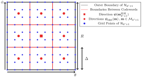
Figure 3: Visualization of the hypothesis grid $\mathcal{H}_{k^{\prime}+1}$ with $H=10$.

The angular spacing between the codewords in $\mathcal{M}_{k^{\prime}+1}$ can be approximated from (6) by evenly dividing the range of the phase difference between the array elements, $A_{\mu}(\bm{\psi})\in[-1,+1],\mu\in\{1,2\}$, by the number of codewords $M$, i.e., $\Delta=\frac{2}{M}\frac{180^{\circ}}{\pi}[\mathrm{deg}]$, ignoring distortions for large angles. Since we consider $2\gamma+1=3$ adjacent codewords for each dimension, the total width of the range of directions that is covered by $\mathcal{M}_{k^{\prime}+1}$ in each dimension is $R=3\Delta$. In order to span the hypothesis space $\mathcal{H}_{k^{\prime}+1}$, we define equally spaced grid points within this range as

$$\small\begin{split}\theta_{h}&=\theta_{\mathrm{IRS}}(\mathbf{m}^{\mathrm{IDE}}_{k^{\prime}+1})-\frac{R}{2}+R\frac{h-1}{H-1},\\ \phi_{h}&=\phi_{\mathrm{IRS}}(\mathbf{m}^{\mathrm{IDE}}_{k^{\prime}+1})-\frac{R}{2}+R\frac{h-1}{H-1},\end{split}$$ (23)

for $h\in\{1,...,H\}$. Finally, $\mathcal{H}_{k^{\prime}+1}$ is defined as $\mathcal{H}_{k^{\prime}+1}=\{(\theta_{h_{1}},\phi_{h_{2}})\,|\,h_{1},h_{2}\in\{1,...,H\}\}$.

III-E Integration of Direction Estimation and User Tracking into Time Block Structure

Now, since all steps of the proposed direction estimation and user tracking algorithm have been introduced, we are ready to summarize the scheme and integrate it into the proposed time block structure. To this end, we first note that in order to initialize the direction estimation in the first TB according to Section III-B, the codebook $\mathcal{M}_{0}$ and the hypothesis set $\mathcal{H}_{0}$ are required. Since for $k^{\prime}=0$, no information about the user’s position at $t_{0}$ is available from previous direction estimates, we assume that some initial access procedure is established to determine $\bm{\mathrm{m}}^{\mathrm{IDE}}_{0}$ from which $\mathcal{M}_{0}$ and $\mathcal{H}_{0}$ are then constructed. $\bm{\mathrm{m}}^{\mathrm{IDE}}_{0}$ can, for example, be obtained by a full codebook search, see [28]. Also, in the same manner, the initial codeword $\bm{\mathrm{m}}^{\mathrm{DT}}_{0}$ can be obtained.

Based on the results from Sections III-B to III-D the proposed IRS-assisted downlink communication scheme is summarized in Algorithm 1.

Algorithm 1 Proposed User-tracking Scheme

1:  Input: $\bm{\mathrm{m}}^{\mathrm{IDE}}_{0}$, $\bm{\mathrm{m}}^{\mathrm{DT}}_{0}$

2:  Initialize: $k=0$

3:  repeat

4:     Select IRS codeword $\mathbf{m}^{\mathrm{DT}}_{k}$ according to (20) or $\mathbf{m}^{\mathrm{DT}}_{0}$ if $k=0$ (UC sub-block).

5:     Determine user combining $\mathbf{f}_{\mathrm{UE}}[k]$ (UC sub-block).

6:     Select $\mathbf{m}^{\mathrm{IDE}}_{k}$ according to (21) or $\mathbf{m}^{\mathrm{IDE}}_{0}$ if $k=0$ and initialize $\mathcal{M}_{k}$ and $\mathcal{H}_{k}$ (IDE sub-block).

7:     Estimate user direction as $\tilde{\bm{\psi}}_{k}$ according to (16) (IDE sub-block).

8:     Compute coefficient matrix $\bm{\mathrm{B}}_{k}$ according to (19) (IDE sub-block).

9:     Set $\kappa=0$

10:     repeat $\eta$ times

11:          Extrapolate user direction as $\widehat{\bm{\mathrm{\psi}}}_{k}(t_{k,\kappa})$ and select $\mathbf{m}^{\mathrm{DT}}_{k,\kappa}$ according to (20).

12:          Perform end-to-end channel estimation (CE sub-block).

13:          Transmit data (DT sub-block).

14:          $\kappa=\kappa+1$

15:     end repeat

16:     $k=k+1$

17:  until User exits the obstructed area.

IV Direction Estimation Codebook Design

The direction estimation and user tracking scheme developed in the previous section is, in general, compatible with any choice of direction estimation codebook $\mathcal{M}_{\mathrm{IDE}}$. So, in principle, one could use the same codebook for direction estimation as for data transmission. However, while the main requirement for the design of the data transmission codebook $\mathcal{M}_{\mathrm{DT}}$ is to maximize the reflection gain, i.e., the signal-to-noise ratio (SNR), the codebook requirements for direction estimation are different (as we will discuss further in this section) and, in general, it is beneficial to use two different codebooks for data transmission and direction estimation, i.e., $\mathcal{M}_{\mathrm{IDE}}\neq\mathcal{M}_{\mathrm{DT}}$. Since no codebook design for IRS-assisted direction estimation is available in the literature, in this paper, we propose a novel codebook design.

To this end, we first propose an approximate theoretical model for the expected direction estimation error for a given codebook. Then, we utilize this model to generate a novel codebook based on a modified beam shape that is specifically optimized for IRS-assisted direction estimation.

IV-A Direction Estimation Error Analysis

According to Section III-D, the range of user directions to be estimated in TB $k$ is $[\theta_{\mathrm{IRS}}(\bm{\mathrm{m}}_{k}^{\mathrm{IDE}})-\frac{3}{2}\Delta,\theta_{\mathrm{IRS}}(\bm{\mathrm{m}}_{k}^{\mathrm{IDE}})+\frac{3}{2}\Delta]\times[\phi_{\mathrm{IRS}}(\bm{\mathrm{m}}_{k}^{\mathrm{IDE}})-\frac{3}{2}\Delta,\phi_{\mathrm{IRS}}(\bm{\mathrm{m}}_{k}^{\mathrm{IDE}})+\frac{3}{2}\Delta]=:\bar{\mathcal{H}}_{k}$. Since the direction estimation problem is identical for any $\bm{\mathrm{m}}_{k}^{\mathrm{IDE}}$, we may assume without loss of generality $\theta_{\mathrm{IRS}}(\bm{\mathrm{m}}_{k}^{\mathrm{IDE}})=\phi_{\mathrm{IRS}}(\bm{\mathrm{m}}_{k}^{\mathrm{IDE}})=0$. Then, the expected squared direction estimation error for a given user position $\bm{\mathrm{\psi}}$ can be written as

$$\mathrm{MSE}_{k}(\bm{\mathrm{\psi}})=\int\limits_{\bar{\mathcal{H}}_{k}}||\bm{\mathrm{\psi}}-\bm{\mathrm{\psi}}^{\prime}||_{2}^{2}\,p_{\tilde{\bm{\psi}}_{k}}(\bm{\mathrm{\psi}}^{\prime})\,\mathrm{d}\bm{\mathrm{\psi}}^{\prime},$$ (24)

where $p_{\tilde{\bm{\psi}}_{k}}(\bm{\mathrm{\psi}}^{\prime})=\frac{\mathrm{d}}{\mathrm{d}\bm{\mathrm{\psi}}^{\prime}}\Pr\left\{\tilde{\bm{\psi}}_{k}\leq\bm{\mathrm{\psi}}^{\prime}\right\}$ and the maximum peak likelihood estimator $\tilde{\bm{\psi}}_{k}$ has been defined in Section III-B. Since we make no prior assumptions with respect to where the user is located within the range of possible directions $\bar{\mathcal{H}}_{k}$, the expected mean squared direction estimation error in $\bar{\mathcal{H}}_{k}$ is given as

$$\mathrm{MSE}_{k}=\frac{1}{\left(3\Delta\right)^{2}}\int\limits_{\bar{\mathcal{H}}_{k}}\mathrm{MSE}_{k}(\bm{\mathrm{\psi}})\,\mathrm{d}\bm{\mathrm{\psi}}.$$ (25)

Here, the challenge for computing (25) lies in evaluating the probability of equivocation $p_{\tilde{\bm{\psi}}_{k}}(\bm{\mathrm{\psi}}^{\prime})$, since $\tilde{\bm{\psi}}_{k}$ is a highly nonlinear function of the noisy direction estimation measurement signal $\bm{\mathrm{r}}_{\bm{\mathrm{m}}}$ as defined in Section III.

In order to develop a first-order approximation for $p_{\tilde{\bm{\psi}}_{k}}(\bm{\mathrm{\psi}}^{\prime})$, let us consider a single codeword $\bm{\mathrm{m}}$ and a given measurement signal $\bm{\mathrm{r}}_{\bm{\mathrm{m}}}$ first. Then, since $\bm{\mathrm{r}}_{\bm{\mathrm{m}}}$ is impaired by white Gaussian noise cf. (11), from all hypothesis directions $\bm{\mathrm{\psi}}^{\prime}$, the maximum likelihood estimate corresponds to the one with the smallest Euclidean distance $||\bm{\mathrm{r}}_{\bm{\mathrm{m}}}-g_{\bm{\mathrm{m}}}(\bm{\mathrm{\psi}}^{\prime})\xi\bm{\mathrm{s}}||_{2}$. Now, since $g_{\bm{\mathrm{m}}}(\bm{\mathrm{\psi}}^{\prime})$ is a continuous function in $\bm{\mathrm{\psi}}^{\prime}$ (according to the steering vectors $\bm{\mathrm{a}}(\bm{\mathrm{\psi}}^{\prime})$ in Section II), it can be approximated as a linear function in a neighborhood of $\bm{\mathrm{\psi}}$, i.e., $g_{\bm{\mathrm{m}}}(\bm{\mathrm{\psi}}^{\prime})=g_{\bm{\mathrm{m}}}(\bm{\mathrm{\psi}})+g_{\bm{\mathrm{m}}}^{\prime}(\bm{\mathrm{\psi}})(\bm{\mathrm{\psi}}-\bm{\mathrm{\psi}}^{\prime})$, where $g_{\bm{\mathrm{m}}}^{\prime}$ denotes the complex-valued derivative of $g_{\bm{\mathrm{m}}}(\bm{\mathrm{\psi}})$ with respect to $\bm{\mathrm{\psi}}$ and we have assumed that $\bm{\mathrm{\psi}}^{\prime}$ is close to $\bm{\mathrm{\psi}}$. In this case, since the complex-valued Gaussian noise in $\bm{\mathrm{r}}_{\bm{\mathrm{m}}}$ is circularly symmetric, it can be decomposed in a component parallel to $g_{\bm{\mathrm{m}}}^{\prime}(\bm{\mathrm{\psi}})$ and a second component that is orthogonal to $g_{\bm{\mathrm{m}}}^{\prime}(\bm{\mathrm{\psi}})$, where both components are zero-mean real-valued Gaussian random variables with variance $\sigma^{2}$. Then, the maximum likelihood estimate of $\bm{\mathrm{\psi}}$ is the projection of $\bm{\mathrm{r}}_{\bm{\mathrm{m}}}$ on the line $c\,g_{\bm{\mathrm{m}}}^{\prime}(\bm{\mathrm{\psi}})$, $c\in\mathbb{R}$, i.e., the probability of equivocation between $\bm{\mathrm{\psi}}$ and $\bm{\mathrm{\psi}}^{\prime}$ is independent of the orthogonal noise component, and we have

$$p_{\tilde{\bm{\psi}}_{k}}(\bm{\mathrm{\psi}}^{\prime})\propto\exp\left(-\frac{||g_{\bm{\mathrm{m}}}(\bm{\mathrm{\psi}})\xi\bm{\mathrm{s}}-g_{\bm{\mathrm{m}}}(\bm{\mathrm{\psi}}^{\prime})\xi\bm{\mathrm{s}}||_{2}^{2}}{2Q_{\mathrm{UE}}\sigma^{2}}\right),$$ (26)

where $\propto$ indicates proportionality. Considering the general case when multiple codewords are available and applying the obtained first-order approximation to (24), we arrive at the following approximation

$$\mathrm{MSE}_{k}(\bm{\mathrm{\psi}}) \approx C_{0}\int\limits_{\bar{\mathcal{H}}_{k}}|\bm{\mathrm{\psi}}-\bm{\mathrm{\psi}}^{\prime}|^{2}$$

$$\quad\prod_{\bm{\mathrm{m}}\in\mathcal{M}_{k}}\exp\left(-\frac{||g_{\bm{\mathrm{m}}}(\bm{\mathrm{\psi}})\xi\bm{\mathrm{s}}-g_{\bm{\mathrm{m}}}(\bm{\mathrm{\psi}}^{\prime})\xi\bm{\mathrm{s}}||_{2}^{2}}{2Q_{\mathrm{UE}}\sigma^{2}}\right)\mathrm{d}\bm{\mathrm{\psi}}^{\prime}$$

$$=:\widehat{\mathrm{MSE}}_{k}(\bm{\mathrm{\psi}}),$$ (27)

where $C_{0}$ is some positive scaling constant. Accordingly, we define the following approximate mean squared direction estimation error for $\bar{\mathcal{H}}_{k}$

$$\widehat{\mathrm{MSE}}_{k}=C_{1}\int\limits_{\bar{\mathcal{H}}_{k}}\widehat{\mathrm{MSE}}_{k}(\bm{\mathrm{\psi}})\,\mathrm{d}\bm{\mathrm{\psi}},$$ (28)

where $C_{1}$ is a positive scaling constant that is irrelevant for the following optimization. We will confirm in Section V that despite the approximate character of (28), it is indeed a useful criterion for practical direction estimation codebook design.

IV-B Beam Shape Optimization

In this section, we leverage the approximation of the direction estimation error derived in the previous section in order to optimize the IRS beam shape $\bm{\mathrm{\omega}}_{\mathcal{M}}$ for direction estimation. The optimal beam shape minimizing $\widehat{\mathrm{MSE}}_{k}$, $\bm{\mathrm{\omega}}_{\mathcal{M}}^{*}$, is defined as follows

$$\bm{\mathrm{\omega}}_{\mathcal{M}}^{*} =\operatorname*{arg\,min}_{\bm{\mathrm{\omega}}_{\mathcal{M}}}\widehat{\mathrm{MSE}}_{k},$$ (29a)

$$\mathrm{s.t.} \quad|[\bm{\mathrm{\omega}}_{\mathcal{M}}]_{i}|^{2}=\bar{g}^{2}\quad\forall\,i,$$ (29b)

with the constant unit cell response factor $\bar{g}$.

Since $\widehat{\mathrm{MSE}}_{k}$ is not a convex function of $\bm{\mathrm{\omega}}_{\mathcal{M}}$, (29) cannot be solved efficiently. However, (29) can still be exploited to find a beam shape that is locally optimal in some neighbourhood of some existing beam shape $\bm{\mathrm{\omega}}_{\mathcal{M}}^{(0)}$, where $\bm{\mathrm{\omega}}_{\mathcal{M}}^{(0)}$ could for example be a linear or a quadratic phase shift profile [18]. To this end, we write

$$\bm{\mathrm{\omega}}_{\mathcal{M}}^{\mathrm{T}}=\bar{g}\cdot[\exp(\mathrm{j}\rho_{1}),\ldots,\exp(\mathrm{j}\rho_{Q})],$$ (30)

and for any beam shape $\bm{\mathrm{\omega}}_{\mathcal{M}}$ define the phase shift function $\rho(\bm{\mathrm{\omega}}_{\mathcal{M}})=[\rho_{1},\ldots,\rho_{Q}]^{T}\in\mathbb{R}^{Q}$ and its inverse function $\rho^{-1}(\cdot)$. Note that constraint (29b) is fulfilled automatically when using (30) to define $\bm{\mathrm{\omega}}_{\mathcal{M}}$.

With these definitions, we equivalently reformulate (29) in terms of $\rho(\bm{\mathrm{\omega}}_{\mathcal{M}})$ and define the locally optimal phase shift vector in the neighborhood of any given phase shifts $\rho\left(\bm{\mathrm{\omega}}_{\mathcal{M}}^{(0)}\right)$ as

$$\rho^{*}\left(\bm{\mathrm{\omega}}_{\mathcal{M}}^{(0)}\right)=\operatorname*{arg\,min}_{\bm{\mathrm{\rho}}_{0}:\left|\left|\bm{\mathrm{\rho}}_{0}-\rho\left(\bm{\mathrm{\omega}}_{\mathcal{M}}^{(0)}\right)\right|\right|_{2}<\delta}\widehat{\mathrm{MSE}}_{k},$$ (31)

where $\bm{\mathrm{\rho}}_{0}\in\mathbb{R}^{Q}$, $\widehat{\mathrm{MSE}}_{k}$ depends on $\bm{\mathrm{\rho}}_{0}$ via the beam pattern $\bm{\mathrm{\omega}}_{\mathcal{M}}=\rho^{-1}(\bm{\mathrm{\rho}}_{0})$, and $\delta>0$ is set small enough such that $\widehat{\mathrm{MSE}}_{k}$ is convex in the considered neighborhood of $\rho\left(\bm{\mathrm{\omega}}_{\mathcal{M}}^{(0)}\right)$. Now, the derivative of $\widehat{\mathrm{MSE}}_{k}$ with respect to each $\rho_{i}$ is computed as follows

$$\frac{\partial}{\partial\rho_{i}} \widehat{\mathrm{MSE}}_{k}\propto-\int\limits_{\bar{\mathcal{H}}_{k}}\int\limits_{\bar{\mathcal{H}}_{k}}||\bm{\mathrm{\psi}}-\bm{\mathrm{\psi}}^{\prime}||^{2}$$

$$\,\times\exp\left(-\frac{||\xi\mathbf{s}||_{2}^{2}}{\sigma^{2}}\sum_{\bm{\mathrm{m}}\in\mathcal{M}_{k}}|\left(\bm{\mathrm{a}}^{\mathrm{H}}(\bm{\mathrm{\psi}})-\bm{\mathrm{a}}^{\mathrm{H}}(\bm{\mathrm{\psi}}^{\prime})\right)\bm{\mathrm{\omega}}(\bm{\mathrm{m}})|^{2}\right)$$

$$\,\times\sum_{\bm{\mathrm{m}}\in\mathcal{M}_{k}}\frac{\partial}{\partial\rho_{i}}|\left(\bm{\mathrm{a}}^{\mathrm{H}}(\bm{\mathrm{\psi}})-\bm{\mathrm{a}}^{\mathrm{H}}(\bm{\mathrm{\psi}}^{\prime})\right)\bm{\mathrm{\omega}}(\bm{\mathrm{m}})|^{2}\,\mathrm{d}\bm{\mathrm{\psi}}\,\mathrm{d}\bm{\mathrm{\psi}}^{\prime},$$ (32)

where we have omitted the proportionality constant and set without loss of generality $\bm{\mathrm{a}}(\bm{\mathrm{\psi}}_{\mathrm{t},1})=\mathbf{1}_{Q^{2}}$. The derivative in the last term of (IV-B) can be further simplified as

$$\frac{\partial}{\partial\rho_{i}}|\left[\bm{\mathrm{a}}(\bm{\mathrm{\psi}})-\bm{\mathrm{a}}(\bm{\mathrm{\psi}}^{\prime})\right]^{\mathrm{H}}\bm{\mathrm{\omega}}(\bm{\mathrm{m}})|^{2}$$

$$=\frac{\partial}{\partial\rho_{i}}|\left[\bm{\mathrm{a}}(\bm{\mathrm{\psi}})-\bm{\mathrm{a}}(\bm{\mathrm{\psi}}^{\prime})\right]^{\mathrm{H}}\left[\left(\bm{\mathrm{\omega}}_{\mathcal{M}}\odot\bm{\mathrm{\omega}}_{m_{1}}\right)\otimes\left(\bm{\mathrm{\omega}}_{\mathcal{M}}\odot\bm{\mathrm{\omega}}_{m_{2}}\right)\right]|^{2}$$

$$=\frac{\partial}{\partial\rho_{i}}|\left[\bm{\mathrm{a}}(\bm{\mathrm{\psi}})-\bm{\mathrm{a}}(\bm{\mathrm{\psi}}^{\prime})\right]^{\mathrm{H}}\left[\left(\bm{\mathrm{\omega}}_{\mathcal{M}}\otimes\bm{\mathrm{\omega}}_{\mathcal{M}}\right)\odot\left(\bm{\mathrm{\omega}}_{m_{1}}\otimes\bm{\mathrm{\omega}}_{m_{2}}\right)\right]|^{2}.$$ (33)

Since in (33) only $\bm{\mathrm{\omega}}_{\mathcal{M}}$ depends on $\rho_{i}$, $\frac{\partial}{\partial\rho_{i}}\widehat{\mathrm{MSE}}_{k}$ can be computed very efficiently using numerical integration. Then, to find ${\rho}^{*}\left(\bm{\mathrm{\omega}}_{\mathcal{M}}^{(0)}\right)$, straightforward gradient descent can be applied as follows

$$[\rho^{(l+1)}_{1},\ldots,\rho^{(l+1)}_{Q}]^{\mathrm{T}}=[\rho^{(l)}_{1},\ldots,\rho^{(l)}_{Q}]^{\mathrm{T}}-w^{l}\zeta\nabla_{\bm{\mathrm{\rho}}}\widehat{\mathrm{MSE}}_{k},$$ (34)

where $l\in\mathbb{N}_{0}$, ${\rho}\left(\bm{\mathrm{\omega}}_{\mathcal{M}}^{(0)}\right)=[\rho^{(0)}_{1},\ldots,\rho^{(0)}_{Q}]^{\mathrm{T}}$, $\zeta$ denotes the step size, $w\in(0,1]$, and (34) is applied until the stopping criterion $||w^{l}\zeta\nabla\widehat{\mathrm{MSE}}_{k}||_{2}<\mu$ is achieved for some $\mu>0$, $l^{\prime}\in\mathbb{N}_{0}$. The locally optimal beam $\bm{\mathrm{\omega}}_{\mathcal{M}}^{*}\left(\bm{\mathrm{\omega}}_{\mathcal{M}}^{(0)}\right)$ is then obtained as $\bm{\mathrm{\omega}}_{\mathcal{M}}^{*}\left(\bm{\mathrm{\omega}}_{\mathcal{M}}^{(0)}\right)=\rho^{-1}\left([\rho^{(l^{\prime})}_{1},\ldots,\rho^{(l^{\prime})}_{Q}]\right)$. We will confirm in the following section that (34) indeed leads to a beam shape that is superior to existing beams in terms of the achieved direction estimation error.

V Performance Evaluation

In the following, the proposed direction estimation and UT schemes are numerically evaluated. First, in Subsection V-A, the direction estimation codebook design presented in Section IV is evaluated considering the direction estimation problem separately. Then, in Subsection V-B, the complete direction estimation and UT scheme as introduced in Section III is numerically evaluated. The simulation parameters used in this section are collected in Table I.

TABLE I: Simulation Settings.

$\mathbf{p}_{\mathrm{BS}}$	$[0,0,10]$ m	$Q_{\mathrm{IRS},1},Q_{\mathrm{IRS},2}$	40, 40	$T$	1.5 s
$\mathbf{p}_{\mathrm{IRS}}$	$[-40,40,5]$ m	$d_{1},d_{2}$	$\lambda/2$	$T_{\mathrm{CE}}+T_{\mathrm{D}}$	1.29 ms
$\mathbf{r}_{\mathrm{C}}$	$[0,40,0]$ m	$Q_{\mathrm{BS}},Q_{\mathrm{UE}}$	16x4 , 2x2	$T_{\mathrm{S}}$	4.16 $\mu$s
$r_{1},r_{2}$	10 m, 5 m	$L_{\mathrm{r}}$, $L_{\mathrm{t}}$	4, 4	$K_{\mathrm{t}},K_{\mathrm{r}}$	10,10
$v$	5 km/h	$S_{\mathrm{max}}$	3	$\sigma^{2}$	- 120 dBm
$N_{\mathrm{IDE}}$	5	$n,\gamma$	1,1	$f_{\mathrm{c}}$	28 GHz

V-A Direction Estimation

In this section, we first present the beam shape generated by the local optimization procedure from Section IV-B. Then, the direction estimation performance of the codebook obtained from this beam is evaluated and compared to benchmark codebooks from the literature.

V-A1 Beam Shape

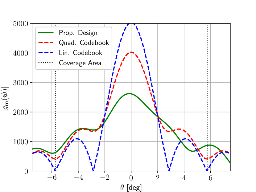
Figure 4: The beam shapes for the proposed direction estimation codebook design (green), the quadratic codebook (red), and the linear codebook (blue) for different horizontal user directions, i.e., different values of $\theta$. Furthermore, the desired coverage area is indicated (dotted vertical lines).

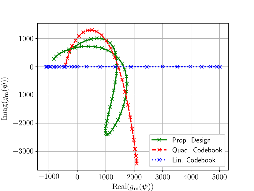
Figure 5: The IRS response function $g_{\bm{\mathrm{m}}}$ in complex coordinates for the proposed direction estimation codebook design (green), the quadratic codebook (red), and the linear codebook (blue).

Fig. 5 shows the beam amplitudes $|g_{\bm{\mathrm{m}}}(\bm{\mathrm{\psi}})|$ for different horizontal directions $\theta$ as generated by the linear codebook, the quadratic codebook [18], and the direction estimation codebook design presented in this paper, all for an IRS of size $Q=40$ and $M=20$. For the proposed design, the quadratic phase shift profile, that is also given as reference, is used as the initial phase shift profile $\bm{\omega}_{\mathcal{M}}^{(0)}$. We observe from Fig. 5 that the direction estimation beam shape proposed in this paper, i.e., $\bm{\mathrm{\omega}}_{\mathcal{M}}^{*}(\bm{\mathrm{\omega}}_{\mathcal{M}}^{(0)})$ as defined in Section IV-B, is broader as compared to the linear and quadratic reference beams. The broad beam shape is intuitively advantageous for direction estimation, since the entire considered direction range is supplied with sufficient power to accurately estimate the user’s actual position. In contrast, the considered reference beams are optimized for data transmission which benefits from a concentrated high SNR at the center of the beam.

Furthermore, we observe from Fig. 5 that the proposed direction estimation beam is asymmetric while the reference beams are perfectly symmetric. To further elucidate this property, the corresponding IRS response functions $g_{\bm{\mathrm{m}}}$ are plotted in Fig. 5 in the complex plane for the same range of $\theta$ and the same three beams as shown in Fig. 5, respectively. Note that for the linear and quadratic codebooks, the $g_{\mathbf{m}}$ for $+\theta$ and $-\theta$ are identical, due to the symmetric design of their respective phase shift profiles. In contrast, we observe from Fig. 5 that the proposed direction estimation beam is not symmetric with respect to the phase of the corresponding $g_{\bm{\mathrm{m}}}$. Intuitively, the phase is exploited as an additional degree of freedom in the proposed direction estimation beam to reduce ambiguities when estimating the user’s direction. Finally, we observe from Figs. 5 and 5 that the maximum gain of the proposed beam is lower than the maximum gains of the reference beams. However, we will confirm in the following section that the negative effect of the smaller amplitude is more than compensated for by the advantages of the asymmetric beam design in terms of the direction estimation performance.

V-A2 Performance

Different codebooks may lead to different reflection gains and therefore different SNRs at the receiver, even if all other system parameters are identical. Hence, to compare the direction estimation performances of different codebooks, we first define the maximum signal-to-noise ratio (MSNR) follows as

$$\mathrm{MSNR}=\frac{\xi^{2}g_{\mathrm{max}}^{2}P_{\mathrm{TX}}}{\sigma^{2}},$$ (35)

where $g_{\mathrm{max}}=\bar{g}Q^{2}$. The MSNR is a codebook independent quantity corresponding to the maximum achievable SNR at the receiver for the optimal IRS phase shift configuration. Then, for several randomly generated test directions $\bm{\mathrm{\psi}}$ within the boundaries of some hypothesis set $\mathcal{H}_{k}$, i.e., $\bm{\mathrm{\psi}}\in\bar{\mathcal{H}}_{k}$, and different codebooks, the IDE as presented in Section III is performed and the squared error $\left\|\tilde{\bm{\mathrm{\psi}}}_{k}-\bm{\mathrm{\psi}}\right\|_{2}^{2}$ is evaluated.

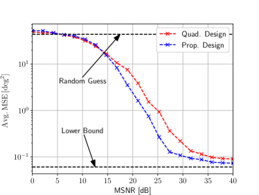
Figure 6: Average direction estimation error for the quadratic (red) and the proposed direction estimation codebook (blue) for different MSNRs.

Fig. 6 shows the average direction estimation error obtained for the quadratic reference codebook and the direction estimation codebook proposed in this paper, respectively. Furthermore, the MSE for a random guess of a point in $\mathcal{H}$ and the lower bound MSE, when always selecting the closest hypothesis direction from $\mathcal{H}_{k}$, are plotted. We note that since for very low MSNRs, the presented direction estimation method tends to mistake the far left and far right sections (with respect to the coverage area) of the considered beams, due to their similar reflection gains, the resulting MSE may be worse than an unbiased random guess in this case.

We observe from Fig. 6 that for increasing MSNR the MSE decreases. This is intuitive, since the noise becomes less detrimental as MSNR increases. Furthermore, we observe from Fig. 6 that the proposed direction estimation codebook outperforms the quadratic reference codebook over a wide range of MSNRs, while both approach the random guess and the lower bound for low and high MSNRs, respectively. This observation confirms that the direction estimation beam shape design presented in Section IV is superior to existing reference beam designs in terms of direction estimation performance.

V-B Performance of UT Scheme

In this section, we compare the average realized SNR during data transmission and the effective rate obtained with the proposed UT algorithm, cf. Section III, and three baseline schemes. For data transmission and direction estimation, we adopt the quadratic codebook design and the proposed direction estimation codebook design, respectively.

Specifically, the SNR is evaluated as

$$\mathrm{SNR}(t)=\frac{|\mathbf{f}_{\mathrm{UE}}^{\mathrm{H}}[k]\mathbf{H}_{\mathrm{r}}\mathbf{\Omega}(\mathbf{m}^{\mathrm{DT}})\mathbf{H}_{\mathrm{t}}\mathbf{f}_{\mathrm{BS}}s(t)|^{2}}{Q_{\mathrm{UE}}\sigma^{2}},$$ (36)

and the effective rate is defined as

$$R(t)=(1-\Gamma)\log_{2}(1+\mathrm{SNR}(t)),$$ (37)

where $\Gamma$ denotes the overhead ratio. The specific value of $\Gamma$ depends on the employed transmission scheme as will be discussed below.

The following three baseline schemes are considered. The focusing baseline has perfect CSI and aligns the reflected beam to the LoS direction at all times. The perfect hierarchical search baseline selects the codeword with the highest reflection gain in regular intervals of $T$ without errors that can be interpreted as an upper bound for hierarchical search. The perfect codebook baseline aligns the IRS with the LoS user direction at all times, which constitutes a theoretical upper bound for codebook-based IRS configuration. For all baselines, the BS and user antenna beamforming are carried out as for the proposed UT scheme. The results have been averaged over 12 different movement trajectories, each simulated 10 times to account for different noise realizations. Simulations in which a permanent user connection could not be maintained by the system were excluded from the evaluation, since those cases would be dealt with on a higher protocol layer than the physical layer in any real-world application. However, the percentage of excluded simulations, denoted as loss probability, is reported for all simulations. The quadratic codebook design is used for all reference schemes and for $\mathcal{M}_{\mathrm{DT}}$ and the proposed codebook design method from section IV is used to generate $\mathcal{M}_{\mathrm{IDE}}$.

V-B1 Overhead

Next, we classify the overhead ratio $\Gamma$ for each of the considered schemes before we discuss the numerical results.

Proposed UT Scheme

We recall from Section II that the duration of the CE sub-block is $T_{\mathrm{CE}}=N_{\mathrm{CE}}T_{\mathrm{S}}$, where $N_{\mathrm{CE}}$ is the number of pilot symbols for the end-to-end channel estimation. Since the parameter estimated in the CE block, $\xi$, is a scalar that does not scale with the number of IRS unit cells, the required number of pilot symbols for channel estimation is constant, e.g., $N_{\mathrm{CE}}\sim\mathcal{O}(1)$, resulting in a short $T_{\mathrm{CE}}$. Overall, for the proposed UT scheme,

$$\Gamma=\frac{T_{\mathrm{UC}}+T_{\mathrm{IDE}}+\eta T_{\mathrm{CE}}}{T}.$$ (38)

Focusing Baseline

The TB structure of the focusing baseline scheme consists of alternating CE and DT sub-blocks, resulting in a relative overhead of:

$$\Gamma_{\mathrm{B}}=\frac{T_{\mathrm{CE}}^{\mathrm{B}}}{T_{\mathrm{CE}}^{\mathrm{B}}+T_{\mathrm{DT}}^{\mathrm{B}}},$$ (39)

where $T_{\mathrm{CE}}^{\mathrm{B}}=N_{\mathrm{CE}}^{\mathrm{B}}T_{\mathrm{S}}$ with pilot sequence length $N_{\mathrm{CE}}^{\mathrm{B}}$. For this baseline, the individual channel of each IRS unit cell ($\mathbf{H}_{\mathrm{r}}$ and $\mathbf{H}_{\mathrm{t}}$), from now on called the full channel, needs to be estimated. The number of unknown channel parameters of the full channel scales with the number of IRS unit cells and conventional channel estimation would require the pilot sequence length to scale with the number of unknown channel parameters. As this is too resource expensive, and potentially infeasible to perform within the channel coherence time, compressed sensing (CS) methods can be used. We do not analyze compressed sensing methods in this paper, but from [29] it can be concluded that the required number of pilot symbols scales as $N_{\mathrm{CE}}^{\mathrm{B}}\sim\mathcal{O}\left(L_{\mathrm{r}}L_{\mathrm{t}}\mathrm{ln}(Q_{\mathrm{IRS}})\right)$.

Hierarchical Search Baseline

For the hierarchical search baseline, we assume that there are $L_{\mathrm{C}}$ codebook levels and each codeword in a lower level covers the range of $N_{\mathrm{HS}}$ codewords in the next level. In the first codebook level, all $M_{\mathrm{HS}}/N_{\mathrm{HS}}^{L_{\mathrm{C}}-1}$ codewords are considered, where $M_{\mathrm{HS}}$ is the size of the final codebook level. In all $L_{\mathrm{C}}-1$ remaining codebook levels, $N_{\mathrm{HS}}$ codewords are considered, if only the best result of the previous level is selected. In summary, the overhead time is given as $T_{\mathrm{HS}}=T_{\mathrm{CE}}\big{(}M_{\mathrm{HS}}/N_{\mathrm{HS}}^{L_{\mathrm{C}}-1}+N_{\mathrm{HS}}(L_{\mathrm{C}}-1)\big{)}$ and, hence,

$$\Gamma_{\mathrm{HS}}=\frac{T_{\mathrm{UC}}+T_{\mathrm{HS}}+\eta_{\mathrm{HS}}T_{\mathrm{CE}}}{T},$$ (40)

where $\eta_{\mathrm{HS}}$ is the number of CE and DT sub-blocks for the hierarchical search baseline.

Perfect Codebook Baseline

The overhead and, hence, the effective rate of the perfect codebook search cannot be determined exactly, since it is a purely theoretical bound with potentially infinite overhead. However, for comparison, in the following we utilize an approximation of the overhead incurred in the perfect codeword selection based on its scaling order. inline]Vahid: Then, do we show effective rate for it? or we treat it as an upperbound? The reader may expect a follow-up sentence here. MG: Is it not clear with the following paragraph? SL: I am also confused here. How can we show the avg. rate in the plot if we cannot determine the overhead?

The exact numerical value of the overhead for each considered scheme depends on many factors in the system model and employed algorithms, which makes it infeasible to obtain. Hence, for the following numerical evaluation, the length of the pilot symbol sequences are approximated by their scaling orders, i.e., $N_{\mathrm{CE}}=1$ for the proposed UT scheme and the perfect hierarchical search baseline and $N_{\mathrm{CE}}^{\mathrm{B}}=L_{\mathrm{r}}L_{\mathrm{t}}\mathrm{ln}(Q_{\mathrm{IRS}})$ for the full CSI estimation in the focusing baseline. For the hierarchical search, we assume a codebook depth of $L_{\mathrm{C}}=2$ and that each codeword in the lower codebook level covers $N_{\mathrm{HS}}=4$ codeword in the succeeding codebook level.

V-B2 User Tracking Evaluation

For the following evaluation, several possible movement trajectories, linear as well as nonlinear movements, were simulated.

Linear Movement

We first consider linear movement, which occurs in many practical scenarios, such as a person traveling along a straight street. Fig. 7(a) illustrates the average SNR during data transmission for the proposed UT scheme and the considered baseline schemes. For the proposed UT scheme, the perfect hierarchical search, and the perfect codebook baseline two different codebook sizes are considered. As expected, the focusing baseline achieves the highest SNR among all considered schemes. This result is intuitive, since the IRS reflection gain is maximized towards the actual LoS user direction in the focusing baseline. For all other schemes, the realizable reflection gain depends on the codebook size. Naturally, a larger codebook enables narrower beams with a larger reflection gain. Consequently, we observe from Fig. 7 that the codebooks of size $M=40$ achieve a higher SNR than those with codebook size $M=30$. For both codebook sizes, the proposed UT scheme performs very close to the optimum, i.e., the perfect codebook baseline, while the performance of the hierarchical search baseline is comparatively worse. This observation is readily explained by the fact that the codeword selection in the hierarchical search baseline is quickly outdated since it is performed only once towards the end of each TB. Furthermore, it can be observed that the loss probability for the proposed UT scheme goes to zero for all but very small transmit powers. Hence, a recovery procedure is not needed to track linear movements.

Fig. 7(b) shows the average effective rate for all considered schemes for different transmit powers. We observe from Fig. 7(b) that, due to its low overhead, the proposed UT scheme outperforms all considered baseline schemes in terms of the average effective rate.

The observations in this section confirm that the key features of the proposed UT scheme, namely the user position extrapolation algorithm presented in Section III and the direction estimation codebook design from Section IV, indeed lead to competitive performance of the proposed scheme when compared to baseline schemes.

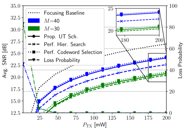
(a)

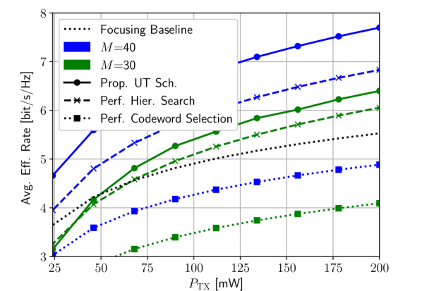
(b)

Figure 7: Performance averaged over several iterations of linear movement. (a) Average SNR. (b) Average effective rate.

Nonlinear Movement

To explore the limits of the proposed UT scheme, we consider now a highly nonlinear movement trajectory, similar to the one introduced in [30]. Specifically, the user is assumed to move inside a circular area with radius $r_{1}$ and center $\mathbf{r}_{\mathrm{C}}$. Starting at a random point on the outer boundary of the blocked area, the user moves linearly towards the center until it reaches a distance of $r_{2}$, $r_{2}<r_{1}$, to the center. Then, it follows a circular trajectory around the center in a counter-clockwise direction. At a randomly determined position, the user again adopts a linear trajectory away from the center until leaving the blocked area. Hence, the user trajectory comprises first a linear, then a nonlinear, and then a second linear part, with abrupt (non-smooth) direction changes between the individual parts.

In Fig. 8(a), the average SNR for nonlinear movement is presented, with otherwise the same simulation setup as for the linear movement evaluated in Fig. 7. We observe from Fig. 8(a) that the average SNR obtained with the proposed UT scheme is still slightly larger than that of the hierarchical search baseline. On the other hand, the gap in terms of SNR to the perfect codebook baseline is increased as compared to the linear movement. In general, a large codebook with narrow beams requires more frequent changes of the employed codeword. Hence, the gain obtained by employing user position extrapolation in the proposed scheme as compared to the perfect hierarchical search baseline is greater for $M$=$40$ than $M$=$30$.

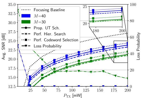
(a)

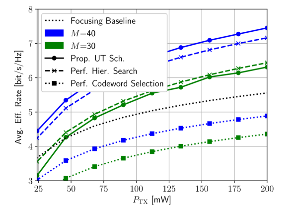
(b)

Figure 8: Performance averaged over several iterations of nonlinear movement. (a) Average SNR. (b) Average effective rate.

The loss probability of the UT algorithm employing the larger codebook is zero for most values of the transmit power, similar to the linear movement case. However, for the smaller codebook, a non-negligible loss probability persists even for large transmit powers. Since the tracking loss of a user is a multi-factorial event, it is in general not possible to attribute it to any single event. However, since no tracking losses occur for the linear movement, some losses in the nonlinear scenario can be attributed to the aforementioned challenges in predicting the nonlinear user trajectory, especially when the user direction changes abruptly, i.e., when the trajectory is highly non-smooth. We will confirm this hypothesis towards the end of this section in the discussion of Fig. 9.

Fig. 8(b) shows the average effective rate for the considered nonlinear movement as a function of the transmit power. We observe from Fig. 8(b) that the focusing baseline performs worse compared to the other considered schemes, similar to the linear movement case. For the larger codebook, the proposed UT scheme still achieves a higher effective rate than the hierarchical search baseline, but the gap is slightly decreased as compared to the linear movement. For the smaller codebook, the average effective rate of the proposed UT scheme is slightly lower compared to the perfect hierarchical search baseline. This happens since the variance of the SNR achieved with the proposed UT scheme is comparatively large, due to potentially incorrect codeword selection leading to large SNR drops. Due to the logarithm in (37), stochastic variations in the SNR are detrimental for the effective rate. On the other hand, wrong codeword selection is not possible by definition for the perfect hierarchical search (rendering its performance as observed in Fig. 8(b) an upper bound for practical schemes based on hierarchical search). Finally, we observe from Fig. 8(b) that the proposed UT scheme always outperforms the perfect codebook baseline in terms of effective rate.

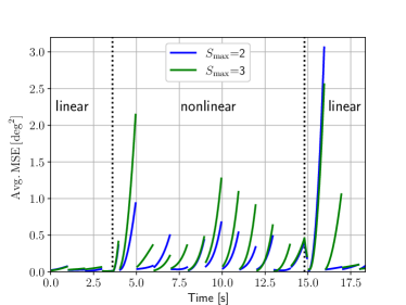
Figure 9: Direction prediction error over time for an exemplary user trajectory realization.

Completing the discussion in this section, we now study the specific challenges for trajectory extrapolation in the considered nonlinear movement scenario in more detail. To this end, Fig. 9 shows the direction prediction error $\left\|\widehat{\bm{\psi}}_{k}(t)-\bm{\psi}_{\mathrm{UE,1}}(t)\right\|_{2}^{2}$ (averaged over several realizations of the noise) for transmit power $P_{\mathrm{TX}}=100\mathrm{mW}$ for an exemplary nonlinear user trajectory. The prediction is regularly updated in the IDE sub-blocks, leading to a comparatively low prediction error directly after each IDE sub-block. As illustrated in Fig. 9, the direction prediction error then increases during the subsequent extrapolation phase (CE, DT, and UC sub-blocks) before decaying again in the next IDE sub-block. We observe from Fig. 9 that, during the initial linear movement section, the prediction works seamlessly, resulting in a low error. However, directly after transitioning to the nonlinear movement section, previous direction estimates are not informative of the new movement trajectory. This leads to comparatively large errors, that reduce again after sufficiently many new direction estimates are obtained. Furthermore, the speed at which the trajectory extrapolation adapts to the altered movement pattern depends on the number of considered past direction estimates $S_{\mathrm{max}}$, namely the prediction error reduces quicker after each transition for $S_{\mathrm{max}}=2$ than for $S_{\mathrm{max}}=3$. Finally, we observe from Fig. 9 that, after transitioning into the second linear movement section, the prediction error first increases (since, as in the first transition, the trajectory at the point of transition is non-smooth) before reducing again to a low value. These observations confirm that the transitions between the different movement patterns as well as the nonlinear part of the user trajectory render the prediction less reliable as compared to the linear movement scenario.

From the results presented in this section, we conclude that the proposed UT scheme still delivers competitive performance both in terms of the average realized SNR and the average effective rate even for nonlinear user movement which is notoriously difficult to predict. Furthermore, it is confirmed that a higher codebook resolution in terms of the number of codewords is required to effectively serve nonlinearly moving users as compared to linear moving ones.

VI Conclusion

In this paper, a novel codebook-based UT algorithm has been presented. Specifically, we introduced a maximum peak likelihood-based direction estimation method and a position extrapolation scheme that tracks general user movements by adapting a trajectory estimate to several past direction measurements. The proposed algorithm utilizes the extrapolated trajectory to predict the future directions of the user and anticipates if a codeword change benefits the average achieved SNR, improving the average SNR compared to baseline schemes with less frequent IRS configuration updates. The impact of the employed IRS codebook on the direction estimation error has been theoretically analyzed and the results of this analysis were utilized to generate a codebook optimized for direction estimation. Our numerical results show that both the proposed UT scheme and the proposed optimized codebook design outperform various baseline schemes. Hence, we believe that the proposed schemes present a significant step towards the effective utilization of IRS-assisted communication systems for serving mobile users with arbitrary movement trajectories.

Interesting topics for further research include the consideration of multiple simultaneously moving users which are served over non-orthogonal channels and the usage of multiple IRSs for user tracking and direction estimation. Also, the integration of neural network based approaches into the proposed UT scheme is a promising avenue for future research.

References

- [1] M. Garkisch, V. Jamali, and R. Schober, “Codebook-based user tracking in IRS-assisted mmwave communication networks,” in Proc. IEEE Int. Conf. Acoust. Speech Signal Process. (ICASSP), June 2023, pp. 1–5.
- [2] M. K. Samimi and T. S. Rappaport, “3-D millimeter-wave statistical channel model for 5G wireless system design,” IEEE Trans. Microw. Theory Techn., no. 7, pp. 2207–2225, Jul. 2016.
- [3] Q. Wu and R. Zhang, “Towards smart and reconfigurable environment: Intelligent reflecting surface aided wireless network,” IEEE Commun. Mag., vol. 58, no. 1, pp. 106–112, Jan. 2020.
- [4] Q. Wu, S. Zhang, B. Zheng, C. You, and R. Zhang, “Intelligent reflecting surface-aided wireless communications: A tutorial,” IEEE Trans. Commun., vol. 69, no. 5, pp. 3313–3351, May 2021.
- [5] M. Najafi, V. Jamali, R. Schober, and V. H. Poor, “Physics-based modeling and scalable optimization of large intelligent reflecting surfaces,” IEEE Trans. Commun., vol. 69, no. 4, pp. 2673–2691, Apr. 2020.
- [6] S. Abeywickrama, R. Zhang, Q. Wu, and C. Yuen, “Intelligent reflecting surface: Practical phase shift model and beamforming optimization,” IEEE Trans. Commun., vol. 68, no. 9, pp. 5849–5863, Sept. 2020.
- [7] Q. Wu and R. Zhang, “Beamforming optimization for wireless network aided by intelligent reflecting surface with discrete phase shifts,” IEEE Trans. Commun., vol. 68, no. 3, pp. 1838–1851, Mar. 2020.
- [8] R. Schmidt, “Multiple emitter location and signal parameter estimation,” IEEE Trans. Antennas Propag., vol. 34, no. 3, pp. 276–280, March 1986.
- [9] C.-B. Ko and J.-H. Lee, “Performance of ESPRIT and Root-MUSIC for angle-of-arrival(AOA) estimation,” in Proc. IEEE World Symp. Commun. Engineer. (WSCE), Dec. 2018, pp. 49–53.
- [10] C. Wang, L. Ma, R. Li, T. S. Durrani, and H. Zhang, “Exploring trajectory prediction through machine learning methods,” IEEE Access, vol. 7, pp. 101 441–101 452, Jul. 2019.
- [11] Y. Lu, W. Wang, X. Hu, P. Xu, S. Zhou, and M. Cai, “Vehicle trajectory prediction in connected environments via heterogeneous context-aware graph convolutional networks,” IEEE Trans. Int. Transport. Sys., vol. 24, no. 8, pp. 8452–8464, Aug. 2023.
- [12] C. Zhang, D. Guo, and P. Fan, “Tracking angles of departure and arrival in a mobile millimeter wave channel,” in Proc. IEEE Int. Conf. Commun. (ICC), 2016, pp. 1–6.
- [13] V. Va, H. Vikalo, and R. W. Heath, “Beam tracking for mobile millimeter wave communication systems,” in Proc. IEEE Global Conf. Signal Inf. Proces. (GlobalSIP), Dec. 2016, pp. 743–747.
- [14] G. Stratidakis, G. D. Ntouni, A. A. Boulogeorgos, D. Kritharidis, and A. Alexiou, “A low-overhead hierarchical beam-tracking algorithm for THz wireless systems,” in Proc. IEEE Eur. Conf. Netw. Commun. (EuCNC), Jun. 2020, pp. 74–78.
- [15] H. Wymeersch and B. Denis, “Beyond 5G wireless localization with reconfigurable intelligent surfaces,” in Proc. IEEE Int. Conf. Commun. (ICC), April 2020, pp. 1–6.
- [16] Z. Huang, B. Zheng, and R. Zhang, “Roadside IRS-aided vehicular communication: Efficient channel estimation and low-complexity beamforming design,” IEEE Trans. Wirel. Commun., vol. 22, no. 9, pp. 5976–5989, Jan. 2023.
- [17] B. Zheng, C. You, and R. Zhang, “Intelligent reflecting surface assisted multi-user OFDMA: Channel estimation and training design,” IEEE Trans. Wirel. Commun., vol. 19, no. 12, pp. 8315–8329, Dec. 2020.
- [18] V. Jamali, M. Najafi, R. Schober, and H. V. Poor, “Power efficiency, overhead, and complexity tradeoff in IRS-assisted communications – quadratic phase-shift design,” IEEE Commun. Lett., vol. 25, no. 6, pp. 2048–2052, Jun. 2021.
- [19] W. R. Ghanem, V. Jamali, M. Schellmann, H. Cao, J. Eichinger, and R. Schober, “Optimization-based phase-shift codebook design for large IRSs,” IEEE Commun. Lett., vol. 27, no. 2, pp. 635–639, Feb. 2023.
- [20] J. Kim, S. Hosseinalipour, A. C. Marcum, T. Kim, D. J. Love, and C. G. Brinton, “Learning-based adaptive IRS control with limited feedback codebooks,” IEEE Trans. Wireless Commun., vol. 21, no. 11, pp. 9566–9581, Nov. 2022.
- [21] G. C. Alexandropoulos, V. Jamali, R. Schober, and H. V. Poor, “Near-field hierarchical beam management for RIS-enabled millimeter wave multi-antenna systems,” in Proc. IEEE 12th Sensor Array and Multichannel Signal Process. Workshop (SAM), June 2022, pp. 460–464.
- [22] S. Mabrouki, I. Dayoub, Q. Li, and M. Berbineau, “Codebook designs for millimeter-wave communication systems in both low- and high-mobility: Achievements and challenges,” IEEE Access, vol. 10, pp. 25 786–25 810, Feb. 2022.
- [23] Q. C. Li, G. Wu, and T. S. Rappaport, “Channel model for millimeter-wave communications based on geometry statistics,” in Proc. IEEE Globecom Workshops, Dec. 2014, pp. 427–432.
- [24] C. You, B. Zheng, and R. Zhang, “Fast beam training for IRS-assisted multiuser communications,” IEEE Wirel. Commun. Lett., vol. 9, no. 11, pp. 1845–1849, Nov. 2020.
- [25] N. Reid and D. Fraser, “Likelihood inference in the presence of nuisance parameters,” Proc. Stat. Prob. Part. Phys. Astron. Cosmology, p. 265, 2003.
- [26] D. Basu, “On the elimination of nuisance parameters,” J. Am. Stat. Assoc., vol. 72, no. 358, pp. 355–366, 1977.
- [27] J. W. Demmel, Applied Numerical Linear Algebra. SIAM, 1997.
- [28] B. Ning, Z. Chen, W. Chen, and Y. Du, “Channel estimation and transmission for intelligent reflecting surface assisted THz communications,” in Proc. IEEE Int. Conf. Commun. (ICC), June 2020, pp. 1–7.
- [29] P. Wang, J. Fang, H. Duan, and H. Li, “Compressed channel estimation for intelligent reflecting surface-assisted millimeter wave systems,” IEEE Signal Process. Lett., vol. 27, pp. 905–909, May 2020.
- [30] S. K. Dehkordi, M. Kobayashi, and G. Caire, “Adaptive beam tracking based on recurrent neural networks for mmWave channels,” in Proc. IEEE 22nd Int. Workshop Signal Process. Adv. Wirel. Commun. (SPAWC), Sep. 2021, pp. 1–5.