Nested traveling wave structures in elastoinertial turbulence

Abstract

Elastoinertial turbulence (EIT) is a chaotic flow resulting from the interplay between inertia and viscoelasticity in wall-bounded shear flows. Understanding EIT is important because it is thought to set a limit on the effectiveness of turbulent drag reduction in polymer solutions. In the present study, we analyze simulations of two-dimensional EIT in channel flow using Spectral Proper Orthogonal Decomposition (SPOD), discovering a family of traveling wave structures that capture the sheetlike stress fluctuations that characterize EIT. The frequency-dependence of the leading SPOD mode contains several distinct peaks and the mode structures corresponding to these peaks exhibit well-defined traveling structures. The structure of the dominant traveling mode exhibits shift-reflect symmetry similar to the viscoelasticity-modified Tollmien–Schlichting (TS) wave, where the velocity fluctuation in the traveling mode is characterized by the formation of large-scale regular structures spanning the channel and the polymeric stress field is characterized by the formation of thin, inclined sheets of high polymeric stress localized at the critical layers near the channel walls. The structures corresponding to the higher-frequency modes have a very similar structure, but nested in a region roughly bounded by the critical layer positions of the next-lower frequency mode. A simple theory based on the idea that the critical layers of mode $\kappa$ form the “walls” for the structure of mode $\kappa+1$ yields quantitative agreement with the observed wave speeds and critical layer positions. The physical idea behind this theory is that the sheetlike localized stress fluctuations in the critical layer prevent velocity fluctuations from penetrating them.

1 Introduction

Adding a tiny amount of high molecular weight polymer to a fluid dramatically reduces turbulent drag (Toms, 1949). Therefore, the polymeric additives are used to reduce pumping costs in pipeline transport of crude oil and home heating and cooling systems, and to reduce fuel transfer time in airplane tank filling (Brostow, 2008). Polymer additives also have been envisioned for flood remediation and enhancement of the drainage capacity of sewer systems (Kumar & Graham, 2023; Bouchenafa et al., 2021; Sellin, 1978). The turbulent flow contains streamwise vortices close to walls, which dominate the near-wall momentum transport and thus the drag. During drag reduction, the polymeric chains get stretched due to turbulence and wrap around the streamwise vortices, weakening them to lead to lower turbulent drag (Li & Graham, 2007; Kim et al., 2007; Graham & Floryan, 2021). However, this suppression of near-wall vortices does not generally lead to full relaminarization, but rather to a limiting state called the maximum drag reduction (MDR) asymptote. Some understanding of this observation has come from the discovery of elastoinertial turbulence (EIT), a complex chaotic flow that is sustained, rather than suppressed by viscoelasticity, and thus helps explain the absence of relaminarization (Samanta et al., 2013; Dubief et al., 2023; Shekar et al., 2019). Nevertheless, the structure and mechanism underlying EIT remain poorly understood and are the topic of the present work.

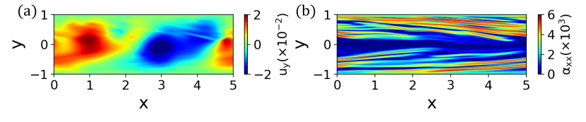
Figure 1: Snapshots of instantaneous (a) wall-normal component of the velocity field ($u_{y}$) and (b) the xx-component of conformation tensor ($\alpha_{xx}$) in EIT at $\Rey=3000$ and $\textit{Wi}=35$.

EIT arises in parameter regimes of Reynolds number $\Rey$ and Weissenberg number Wi (product of polymer relaxation time and nominal strain rate) where the laminar flow is linearly stable and is thus a nonlinearly self-sustaining flow. The basic structure in both channel and pipe flows (Samanta et al., 2013; Lopez et al., 2019) is two-dimensional (2D) (Sid et al., 2018), characterized by vorticity fluctuations localized in narrow regions near the walls with tilted sheets of highly stretched polymers emanating from these regions. Figure 1 shows a snapshot of EIT structure in channel flow.

Despite the absence of an obvious linear instability mechanism for EIT, it has been hypothesized that EIT is related to the nonlinear excitation of either a “wall mode” or a “center mode” structure arising in the linear stability problem for the laminar state (Drazin & Reid, 1981; Datta et al., 2022). A wall mode has a wave speed much less than the centerline velocity, and critical layer positions, i.e. where the wave speed equals the local laminar velocity, near the walls. In contrast, a center mode travels at nearly the centerline velocity and accordingly the critical layer position is near the centerline. The Tollmien-Schlichting (TS) mode of classical linear analysis of plane Poiseiulle flow is a wall mode, and there is a strong structural resemblance of the viscoelastic extension of the TS wave to EIT (Shekar et al., 2019, 2020, 2021). Figure 2 shows the viscoelastic linear TS mode at the same conditions as Figure 1. Sheets of highly stretched polymer are generated in the TS wave due to the presence of hyperbolic stagnation points (in the frame traveling with the wave) in the Kelvin cat’s-eye structure of the velocity field in the critical layer (Shekar et al., 2019). The possibility of a center mode structure is of interest in part because there is a linear center mode instability at low Reynolds number $\Rey$ that may organize “elastic turbulence” at very small Reynolds number $\Rey$ (Garg et al., 2018; Khalid et al., 2021; Choueiri et al., 2021; Morozov, 2022). Nevertheless, in the elastoinertial regime considered here, while center mode structures can exist (Dubief et al., 2022), they do not appear to play an active role in the structure and self-sustenance of EIT (Beneitez et al., 2024). The present work is consistent with this picture, and indeed deepens the connection between EIT and wall modes, showing in particular the existence of a nested family of such structures.

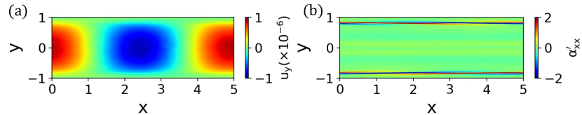
Figure 2: Structures of (a) wall-normal velocity ($u_{y}$) and (b) the perturbation of the xx-component of conformation tensor from mean ($\alpha_{xx}^{\prime}$) of viscoelastic linear TS wave at $Re=3000$ and $Wi=35$. This mode ultimately vanishes as viscoelastic channel flow is linearly stable at this parameter regime.

In the present study, we investigate the structure and dynamics of EIT in channel flow using a modal decomposition technique known as spectral proper orthogonal decomposition (SPOD) (Towne et al., 2018). SPOD characterizes coherent structures in complex flows that have well-defined structures and persist both in space and time via a frequency-domain variant of Proper Orthogonal Decomposition (POD) (Lumley, 1967). At a given frequency, SPOD generates an energetically ordered and spatially orthogonal set of modes characterizing the flow. The modes and eigenvalues obtained using SPOD analysis can be interpreted as physical structures and the energy associated with those structures (Schmidt & Towne, 2019). SPOD has been successfully used in inertial turbulence to understand coherent structures and develop a low-dimensional model for turbulence (Schmidt et al., 2017; Araya et al., 2017; Tutkun & George, 2017; Braud et al., 2004; Hellström & Smits, 2014; Nekkanti & Schmidt, 2021). Here, we use it to investigate traveling coherent structures underlying the chaotic dynamics of EIT. We will focus on the frequency-dependence of the most energetic SPOD mode, as it reveals important coherent features of the flow.

2 Formulation and governing equations

Because the self-sustaining dynamics of elastoinertial turbulence are fundamentally 2D (Sid et al., 2018), we consider two-dimensional (2D) viscoelastic channel flow with nondimensional equations of mass and momentum conservation:

$$\nabla\cdot\bm{u}=0,\ \ \ \ \ \ \frac{\partial\bm{u}}{\partial t}+\bm{u}\cdot\nabla\bm{u}=-\nabla p+\frac{\beta}{Re}\nabla^{2}\bm{u}+\frac{1-\beta}{Re}\nabla\cdot\bm{\tau_{p}}+f(t)\bm{e}_{x},$$ (1)

where $\bm{u}$ and $p$ are non-dimensional velocity field and pressure field, respectively. Laminar centerline velocity ($U_{c}$) and channel half width ($H$) have been used as characteristic velocity scale and length scale, respectively. The ratio between solvent viscosity ($\eta_{s}$) to zero shear rate solution viscosity ($\eta$) has been denoted by $\beta=\eta_{s}/\eta$. The Reynolds number has been defined as $Re=\rho U_{c}H/\eta$, where $\rho$ represents fluid density. We use no-slip boundary conditions for the velocity field at the channel wall. Periodic boundary conditions have been used at the inlet and outlet of the channel. Flow is driven by an external forcing term $f(t)\bm{e}_{x}$, where $\bm{e}_{x}$ denotes the streamwise direction. The forcing term varies with time to keep the volumetric flow rate at its laminar value. The polymer stress tensor is denoted $\bm{\tau_{p}}$ and we choose the FENE-P constitutive model with an artificial diffusion term to model its evolution:

$$\frac{\partial\bm{\alpha}}{\partial t}+\bm{u}\cdot\nabla\bm{\alpha}-\bm{\alpha}\cdot\nabla\bm{u}-(\bm{\alpha}\cdot\nabla\bm{u})^{T}=-\bm{\tau_{p}}+\frac{1}{ReSc}\nabla^{2}\bm{\alpha},$$ (2)

$$\bm{\tau_{p}}=\frac{1}{\textit{Wi}}\left(\frac{\bm{\alpha}}{1-tr(\bm{\alpha})/b}-\bm{I}\right),$$ (3)

where $\bm{\alpha}$ is the conformation tensor and parameter $b$ characterizes the maximum extensibility of the polymeric chains. The Weissenberg number $\textit{Wi}=\lambda U_{c}/H$, where $\lambda$ is the polymeric relaxation time. The Schmidt number $Sc=\eta/\rho D$, where $D$ is the diffusion coefficient, represents the ratio of momentum diffusivity to mass diffusivity. The artificial diffusion term is used to stabilize the numerical scheme during the integration of Eq. 2. The presence of this term leads to the requirement of boundary conditions for the conformation tensor. At the channel walls, we determine $\bm{\alpha}$ by solving the governing equations considering $Sc\to\infty$.

We solve the governing equations with a spectral method using the Dedalus framework (Burns et al., 2020). The computational domain has a length $L=5$. The governing equations have been discretized using 256 Fourier basis functions and 1024 Chebyshev basis functions in the streamwise ($x$) and wall-normal ($y$) directions, respectively. We use $\beta=0.97$, $b=6400$, $Re=3000-6000$, and $\textit{Wi}=35-70$, which are relevant to turbulent drag reduction and are in the range of values used in previous studies, e.g. (Shekar et al., 2019; Dubief et al., 2022). In reality, the Schmidt number for a polymer solution is very large ($Sc\sim 10^{6}$). Numerical simulation with such a large value of $Sc$ would require an extremely fine mesh and small time-step, making numerical simulations computationally very expensive. At the same time, small $Sc$ (i.e., $Sc<10$) smears out small-scale dynamics and suppresses EIT (Sid et al., 2018; Dubief et al., 2023). Therefore, numerical simulations of EIT based on artificial diffusion generally use $Sc\sim O(100)$ (Sid et al., 2018; Buza et al., 2022). In the present study, we use $Sc=100$ which is sufficient to sustain EIT and also numerically tractable. Viscoelastic channel flow in the parameter regime considered here is linearly stable. Therefore, we provide random perturbations to the conformation tensor to initiate EIT. In computing statistics, initial transients are dropped so that we consider only statistically stationary results.

For the SPOD analysis, we use the MATLAB tool developed by Schmidt (2022). Details of the method and its numerical implementation can be found in literature (Towne et al., 2018; Schmidt & Colonius, 2020). We use $300$ time units of data generated using EIT simulation to perform SPOD analysis, which is sufficient for the convergence of SPOD. The data set consists of $N_{t}=4000$ snapshots, which are sampled at the interval of $\Delta t_{s}=0.075$ time units. To obtain converged spectral densities, multiple realizations of the flow are used (Bendat & Piersol, 2000). This can be achieved by dividing the data set into multiple overlapping blocks (Welch, 1967). In the present study, we use $N_{f}=500$ snapshots in each block with $50\%$ overlap, which leads to a total of $N_{b}=15$ blocks. The number of modes obtained in SPOD is the same as the number of blocks, where the first mode has the highest energy and the last mode has the lowest energy. The number of non-negative frequencies is given by $N_{f}/2+1$ and the interval between them is $\Delta f=1/(\Delta t_{s}N_{f})$.

3 Results and discussion

This study focuses on the case $\Rey=3000,\textit{Wi}=35$, for which a snapshot of the wall-normal velocity $u_{y}$ and $xx$ polymer stretch $\alpha_{xx}$ are shown in Figure 1. Results obtained for $\Rey=3000,\textit{Wi}=70$ and $\Rey=6000,\textit{Wi}=35$ display nearly identical features. The dynamics of $u_{y}$ in EIT are dominated by the downstream advection of large-scale structures spanning the channel (Supplementary video: Movie1), whereas the dynamics of the polymeric stress field are dominated by the flapping of thin inclined sheets of polymeric stress in the vicinity of the channel walls (Supplementary video: Movie2). We note that the velocity fluctuations at EIT are generally quite small (e.g. $u_{y}\sim 10^{-2}$), so the velocity profile does not greatly differ from laminar. Since $u_{y}$ is identically zero in the laminar state, it is the most straightforward velocity component to analyze with SPOD. Additionally, most of the polymer stretching in EIT is in the $x$-direction, so our SPOD analyses will consider $u_{y}$ and $\alpha_{xx}^{\prime}$, where $(^{\prime})$ denotes deviation from the mean.

SPOD energy spectra as a function of frequency for the first several modes in $u_{y}$ and $\alpha_{xx}^{\prime}$ are shown in Fig. 3(a) and Fig. 3(b), respectively, along with the energy of the sum of all modes. The SPOD analyses of $u_{y}$ and $\alpha_{xx}^{\prime}$ have been done separately. For wall-normal velocity, the leading mode contains most of the energy ($\approx 75\%$) and hence dominates the flow structure (Fig. 3(a)). In the energy spectrum of $\alpha_{xx}^{\prime}$, the leading mode has a relatively smaller contribution to the total energy ($\approx 32\%$). The leading mode of wall-normal velocity contains distinct peaks at specific frequencies indicated with red symbols, and the energy of these peaks decreases as the frequency increases. The higher-order modes do not have such distinct peaks.

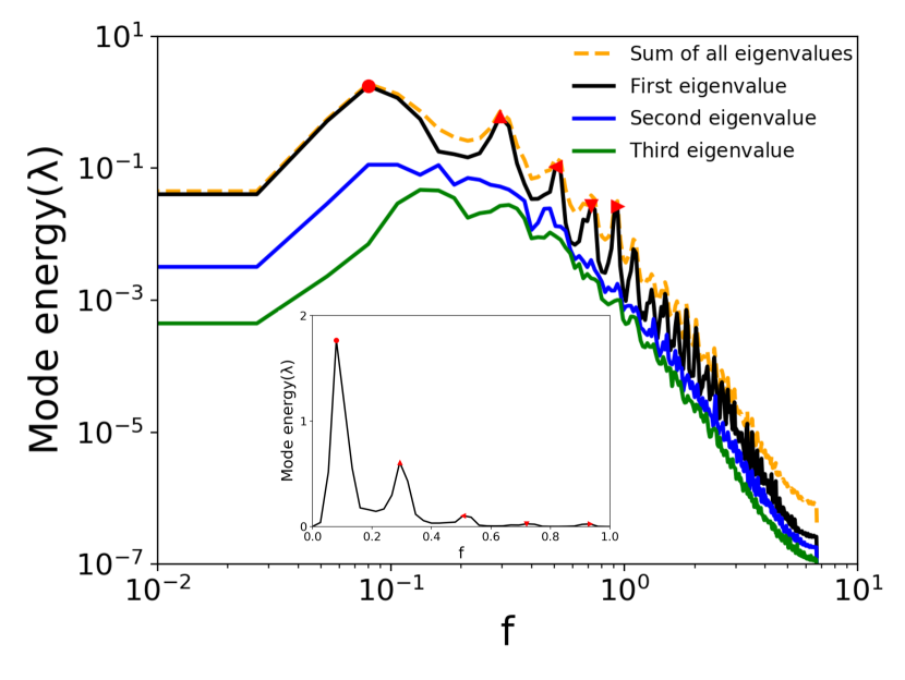
(a)

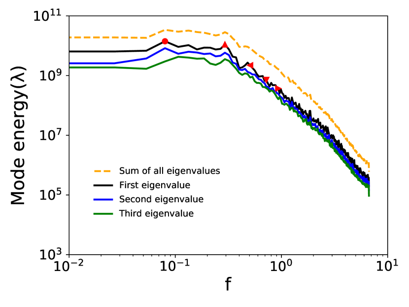
(b)

Figure 3: SPOD energy spectra of (a) wall-normal velocity ($u_{y}$) and (b) the perturbation of the xx-component of conformation tensor ($\alpha_{xx}^{\prime}$) at $\Rey=3000$ and $\textit{Wi}=35$. Red symbols indicate the first few peaks in the leading mode of the energy spectrum of $u_{y}$. Inset of (a): SPOD energy spectrum of the leading SPOD mode for $u_{y}$ on a linear scale.

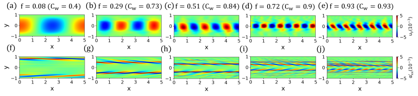
Figure 4: Structures of SPOD modes of (a-e) $u_{y}$ and (f-j) $\alpha_{xx}^{\prime}$ corresponding to the frequencies denoted by different symbols in the energy spectra (Figs. 3(a) and 3(b)).

The local peaks in the energy spectrum of wall-normal velocity indicate that the structures corresponding to these frequencies have distinct features in the dynamics of EIT. These peaks are not at integer multiples of the lowest-frequency peak, so are not simply harmonics; the relationship between them is elucidated below. The SPOD mode structures of $u_{y}$ and $\alpha_{xx}^{\prime}$ corresponding to the peak frequencies in the leading mode of the wall-normal velocity have been shown in Fig. 4. Each mode has a distinct wavenumber $\kappa$, which we measure in wavelengths per domain length. These modes are all traveling waves with wave speed $C_{w}=fL/\kappa$, as further discussed below.

The most dominant SPOD structure ($f=0.08$) has unit wavenumber ($\kappa=1$). The velocity field for this mode consists of large-scale structures spanning the channel (Fig. 4a), and the polymeric stress field displays thin layers close to the walls having inclined alternating sheets of positive and negative stress fluctuations (Fig. 4f). The structures approximately obey a shift-reflect symmetry: i.e. $u_{y}(x,y)\approx-u_{y}(x+L/2,-y)$ and $\alpha_{xx}^{\prime}(x,y)\approx\alpha_{xx}^{\prime}(x+L/2,-y)$. This is the symmetry obeyed by the TS mode (Drazin & Reid, 1981), and comparison to Figure 2 indicates a strong similarity in structure. From here onward, we refer to the regions having positive and negative $u_{y}$ as “positive lobe” and “negative lobe”, respectively. The mode structures corresponding to other peaks have similar structures, where the wavenumber of structures increases with frequency (Fig. 4). The spanwise extent of the lobes in the velocity field decreases as the wavenumber increases. Relatedly, the layers of strong $\alpha_{xx}^{\prime}$ move away from the wall as the frequency increases.

The wave speeds of the traveling structures in the leading SPOD mode are shown in Figure 5(a). They initially increase with the wavenumber (and frequency) and ultimately saturate to a value close to the centerline velocity of the channel ($C_{w}\to 0.94$). The wave speed of the dominant mode ($f=0.08,\kappa=1$) is very close to that of the Newtonian nonlinear TS (NNTS) wave at the corresponding Re ($C_{TS}=0.42$), shown in red on Figure 5(a), further strengthening the evidence connecting EIT to the TS mode. By contrast, a center mode would have a wave speed close to unity and thus a frequency close to $\kappa/L$. For $L=5$ this would be multiples of $0.2$, and examining Figure 3(a) shows no peaks at these positions. In fact, $f=0.2$ and its multiples are close to local minima in energy for the dominant mode. In short, we see no evidence of a center mode structure. We elaborate below on the origin of the peak positions in Figure 3(a).

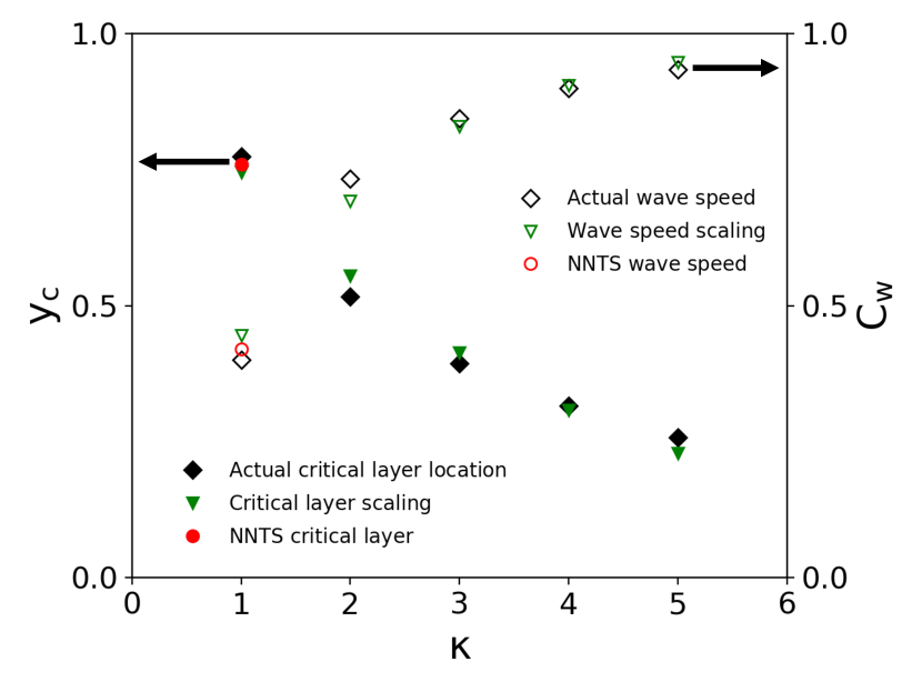
(a)

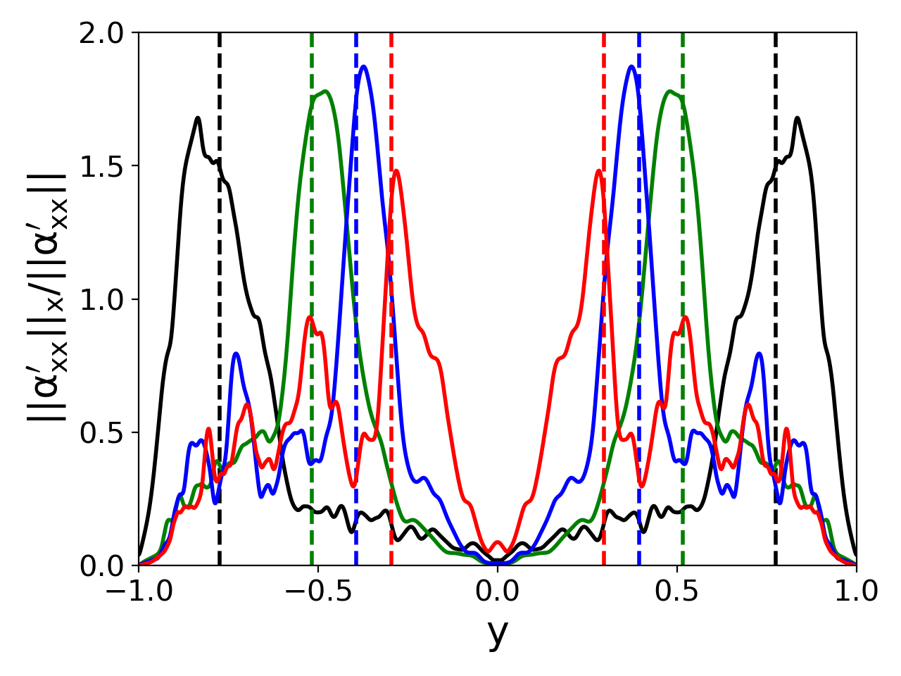
(b)

Figure 5: (a) Wave speed and location of the critical layer for the traveling waves associated with the peaks in the leading SPOD mode along with the Newtonian nonlinear Tollmien–Schlichting (NNTS) mode results and the predictions of the scaling model Eqs. 4 and 5. (b) Streamwise averaged $L_{2}$ norm of $\alpha_{xx}^{\prime}$ (solid lines) and critical layers (dashed lines) for traveling modes having wave speed $C_{w}=0.4$ (black), $C_{w}=0.73$ (green), $C_{w}=0.84$ (blue), and $C_{w}=0.9$ (red).

As discussed in the Introduction, corresponding to the wave speed of a perturbation there is a critical layer position $y_{c}$. As this is the position where the fluid and the perturbation are moving together, it is the most favorable position for the two to exchange energy. The velocity fluctuations in EIT are very weak so the local streamwise velocity $u_{x}\approx 1-y^{2}$, and the location of critical layers can be given as $y_{c}\approx\pm\sqrt{1-C_{w}}$. Figure 5(a) shows the critical layer positions corresponding to the wave speeds of the traveling structures of the leading SPOD mode, as well as for the NNTS mode. As with wave speed, the critical layer position of the $f=0.08,\kappa=1$ SPOD mode is very close to that of the NNTS mode. To explore the relation between the critical layer and the location of the polymeric sheets in the SPOD structures, in Figure 5(b) we plot the streamwise averaged $L_{2}$ norm of $\alpha_{xx}^{\prime}$ ($||\alpha_{xx}^{\prime}||_{x}$) along with the positions of the critical layers for the traveling structures of the dominant SPOD mode. The peak regions represent the locations of the sheets of polymer stretching, and we see that their locations correspond to the critical layers. A similar observation has been made for viscoelasticity-modified TS waves and it has been reported that thin sheets of high polymeric stress emanate from the critical layers of TS waves (Shekar et al., 2019; Hameduddin et al., 2019).

We noted above that as the wavenumber increases, $u_{y}$ becomes more localized toward the channel center, as do the critical layer positions where the stress fluctuations are high. More specifically, consider the $u_{y}$ profile at the second peak ($f=0.29$, Figure 4b) and the $\alpha_{xx}^{\prime}$ profile at the first peak ($f=0.08$, Figure 4f). It appears that the “lobes” where $u_{y}$ is large in the former figure are roughly bounded by the layers where $\alpha_{xx}^{\prime}$ is large in the latter. Similar observations can be made about all of the succeeding modes. We visualize this point in Figure 6, which replots the results of Figure 4 by showing contour lines of $u_{y}$ from the SPOD modes at wavenumber $\kappa+1$ juxtaposed with color contours of $\alpha_{xx}^{\prime}$ at wavenumber $\kappa$. From this figure, we see that the velocity lobes at wavenumber $\kappa+1$ are “nested” within the stress fluctuations, or equivalently between the upper and lower critical layer positions, at wavenumber $\kappa$. In contrast, the regions between the critical layers and the channel walls contain small-scale and irregular structures both in the velocity field as well as stress field.

The nested nature of the structures revealed by SPOD suggests that the locations of the polymeric sheets of a slow-moving (low wavenumber) traveling wave act like “walls” for the immediately faster-moving (and higher wavenumber) wave. Consider the existence of a “primary” mode with wave speed $C_{w,1}$ and thus critical layer positions $y_{c,1}=\pm(1-C_{w,1})^{1/2}$. We take the next higher mode to occupy the domain $|y|<|y_{c,1}|$; if its critical layer position $y_{c,2}$ is at the same fractional position in this new domain, it will thus be at $\pm|y_{c,1}|^{2}=\pm(1-C_{w,1})^{1}$. Continuing in this way, and noting that successively higher-speed waves can be labeled by their wavenumber $\kappa$, we have a simple scaling result

$$y_{c,\kappa}=(1-C_{w,1})^{\kappa/2}.$$ (4)

Relatedly, the successive wave speeds are then

$$C_{w,\kappa}=1-(1-C_{w,1})^{\kappa}.$$ (5)

Using the SPOD results for $y_{c,\kappa}$ to find a best-fit value of $C_{w,1}$ yields predictions for $y_{c,\kappa}$ and $C_{w,\kappa}$ that agree very closely with the data, as shown in Figure 5(a). Furthermore, the value of $C_{w,1}=0.44$ is very close to the NNTS wave speed $C_{TS}=0.42$. These observations indicate that the structure of EIT is dominated by nested structures that closely resemble TS waves.

Finally, we briefly describe a possible mechanism for the appearance of this nested structure. A highly stretched elastic sheet resists lateral deformation. Similarly, flows in which polymer molecules are strongly stretched along one direction resist deformations transverse to that direction. A classical example of this mechanism is the suppression of shear-layer instability in a viscoelastic fluid, where the strong stretching in the shear layer mimics an elastic sheet (Azaiez & Homsy, 2006). Relatedly, viscoelastic Taylor-Couette instability is suppressed by axial flow (Graham, 1998), and in porous media flows, sheetlike regions with high polymeric stress resist the flow passing through them and hence act like flow barriers (Kumar et al., 2023). A similar mechanism is likely at work here, in which the sheets of high polymer stretch in the critical layers from the primary mode prevent velocity fluctuations from the higher modes from passing through the critical layer, acting as “walls” as noted above, and so on successively with the higher modes.

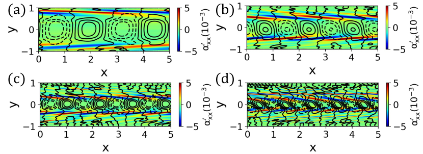
Figure 6: Contours of velocity fluctuations ($u_{y}$) of a faster-traveling wave on the top of the stress fluctuations of the immediate slower traveling wave: (a) stress at $C_{w}=0.4$ and velocity at $C_{w}=0.73$, (b) stress at $C_{w}=0.73$ and velocity at $C_{w}=0.84$, (c) stress at $C_{w}=0.84$ and velocity at $C_{w}=0.9$, and (d) stress at $C_{w}=0.9$ and velocity at $C_{w}=0.93$.

For completeness, we also report in Figure 7 the structure corresponding to the second-most energetic mode from SPOD (blue curve on Figure 3(a)) at $f=0.08$. Note that the energy of this mode is more than an order of magnitude smaller than that of the leading mode and that the spectrum of this structure does not contain distinct peaks. This mode also has $\kappa=1$ and thus the same wave speed and critical layer position as the most energetic mode. It again exhibits localized polymer stretch fluctuations in the critical layer, but now displays simple reflection symmetry rather than the shift-reflect symmetry of the dominant mode. We view this as a higher-order correction on the dominant structure elucidated above.

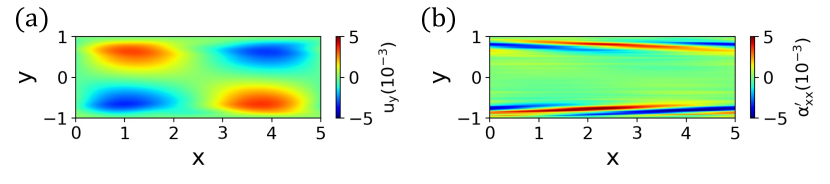
Figure 7: Mode structures the second-most energetic mode at $f=0.08$; (a) $u_{y}$, (b) $\alpha_{xx}^{\prime}$.

4 Conclusions

In the present study, we use Spectral Proper Orthogonal Decomposition (SPOD) to elucidate the structure underlying the chaotic dynamics of elastoinertial turbulence in channel flow. The SPOD energy spectrum of wall-normal velocity for the most energetic structure has distinct peaks. The mode structures corresponding to these peaks exhibit a family of well-defined traveling structures, where the velocity field contains large-scale regular patterns and the polymeric stress field contains the formation of thin inclined sheets of high and low stress at the critical layers of the wave. The structure of the most dominant traveling wave (first, highest peak) of this family exhibits shift-reflect symmetry and resembles the structure of the Tollmien–Schlichting wave indicating its origin in a nonlinearly self-sustained wall mode. The traveling structures corresponding to the higher frequency peaks have very similar structure and symmetry, however, their wavenumber increases, and the size of large-scale structures decreases. We discover that the formation of polymeric sheets at the critical layers acts like walls for the traveling structure of the next higher wave number and hence leads to a nested arrangement of the waves. Based on this observation, a simple theory quantitatively captures the relationship between the wave speeds and the locations of critical layers for different waves. From this analysis, a picture emerges of EIT as a nested collection of nonlinearly self-sustaining TS-wave-like structures.

References

- Araya et al. (2017) Araya, Daniel B., Colonius, Tim & Dabiri, John O. 2017 Transition to bluff-body dynamics in the wake of vertical-axis wind turbines. Journal of Fluid Mechanics 813, 346–381.
- Azaiez & Homsy (2006) Azaiez, J & Homsy, G M 2006 Linear stability of free shear flow of viscoelastic liquids. Journal of Fluid Mechanics 268 (-1), 37 69.
- Bendat & Piersol (2000) Bendat, Julius S & Piersol, Allan G 2000 Random data analysis and measurement procedures. Measurement Science and Technology 11 (12), 1825–1826.
- Beneitez et al. (2024) Beneitez, Miguel, Page, Jacob, Dubief, Yves & Kerswell, Rich R. 2024 Multistability of elasto-inertial two-dimensional channel flow. Journal of Fluid Mechanics 981, A30, arXiv: 2308.11554.
- Bouchenafa et al. (2021) Bouchenafa, Walid, Dewals, Benjamin, Lefevre, Arnaud & Mignot, Emmanuel 2021 Water Soluble Polymers as a Means to Increase Flow Capacity: Field Experiment of Drag Reduction by Polymer Additives in an Irrigation Canal. Journal of Hydraulic Engineering 147 (8), 1–9.
- Braud et al. (2004) Braud, Caroline, Heitz, Dominique, Arroyo, Georges, Perret, Laurent, Delville, Joël & Bonnet, Jean-Paul 2004 Low-dimensional analysis, using POD, for two mixing layer–wake interactions. International Journal of Heat and Fluid Flow 25 (3), 351–363.
- Brostow (2008) Brostow, Witold 2008 Drag reduction in flow: Review of applications, mechanism and prediction. Journal of Industrial and Engineering Chemistry 14 (4), 409–416.
- Burns et al. (2020) Burns, Keaton J., Vasil, Geoffrey M., Oishi, Jeffrey S., Lecoanet, Daniel & Brown, Benjamin P. 2020 Dedalus: A flexible framework for numerical simulations with spectral methods. Physical Review Research 2 (2), 023068, arXiv: 1905.10388.
- Buza et al. (2022) Buza, Gergely, Beneitez, Miguel, Page, Jacob & Kerswell, Rich R. 2022 Finite-amplitude elastic waves in viscoelastic channel flow from large to zero Reynolds number. Journal of Fluid Mechanics 951, A3, arXiv: 2202.08047.
- Choueiri et al. (2021) Choueiri, George H., Lopez, Jose M., Varshney, Atul, Sankar, Sarath & Hof, Björn 2021 Experimental observation of the origin and structure of elastoinertial turbulence. Proceedings of the National Academy of Sciences 118 (45), e2102350118, arXiv: 2103.00023.
- Datta et al. (2022) Datta, Sujit S., Ardekani, Arezoo M., Arratia, Paulo E., Beris, Antony N., Bischofberger, Irmgard, McKinley, Gareth H., Eggers, Jens G., López-Aguilar, J. Esteban, Fielding, Suzanne M., Frishman, Anna, Graham, Michael D., Guasto, Jeffrey S., Haward, Simon J., Shen, Amy Q., Hormozi, Sarah, Morozov, Alexander, Poole, Robert J., Shankar, V., Shaqfeh, Eric S. G., Stark, Holger, Steinberg, Victor, Subramanian, Ganesh & Stone, Howard A. 2022 Perspectives on viscoelastic flow instabilities and elastic turbulence. Physical Review Fluids 7 (8), 080701, arXiv: 2108.09841.
- Drazin & Reid (1981) Drazin, PG & Reid, WH 1981 Hydrodynamic stability (cambridge university .
- Dubief et al. (2022) Dubief, Y, Page, J, Kerswell, R R, Terrapon, V E & Steinberg, V 2022 First coherent structure in elasto-inertial turbulence. Physical Review Fluids 7 (7), 073301.
- Dubief et al. (2023) Dubief, Yves, Terrapon, Vincent E & Hof, Björn 2023 Elasto-Inertial Turbulence. Annual Review of Fluid Mechanics 55 (1), 675–705.
- Garg et al. (2018) Garg, Piyush, Chaudhary, Indresh, Khalid, Mohammad, Shankar, V. & Subramanian, Ganesh 2018 Viscoelastic Pipe Flow is Linearly Unstable. Physical Review Letters 121 (2), 24502, arXiv: 1711.07991.
- Graham (1998) Graham, Michael D 1998 Effect of axial flow on viscoelastic Taylor-Couette instability. Journal of Fluid Mechanics 360, 341 374.
- Graham & Floryan (2021) Graham, Michael D. & Floryan, Daniel 2021 Exact Coherent States and the Nonlinear Dynamics of Wall-Bounded Turbulent Flows. Annual Review of Fluid Mechanics 53 (1), 227–253.
- Hameduddin et al. (2019) Hameduddin, Ismail, Gayme, Dennice F. & Zaki, Tamer A. 2019 Perturbative expansions of the conformation tensor in viscoelastic flows. Journal of Fluid Mechanics 858, 377–406, arXiv: 1811.02501.
- Hellström & Smits (2014) Hellström, Leo H. O. & Smits, Alexander J. 2014 The energetic motions in turbulent pipe flow. Physics of Fluids 26 (12).
- Khalid et al. (2021) Khalid, Mohammad, Chaudhary, Indresh, Garg, Piyush, Shankar, V. & Subramanian, Ganesh 2021 The centre-mode instability of viscoelastic plane Poiseuille flow. Journal of Fluid Mechanics 915, A43, arXiv: 2008.00231.
- Kim et al. (2007) Kim, Kyoungyoun, Li, Chang-F., Sureshkumar, R., Balachandar, S. & Adrian, Ronald J. 2007 Effects of polymer stresses on eddy structures in drag-reduced turbulent channel flow. Journal of Fluid Mechanics 584, 281–299.
- Kumar & Graham (2023) Kumar, Manish & Graham, Michael D. 2023 Effect of polymer additives on dynamics of water level in an open channel. Journal of Non-Newtonian Fluid Mechanics 321 (June), 105129, arXiv: 2307.00626.
- Kumar et al. (2023) Kumar, Manish, Guasto, Jeffrey S. & Ardekani, Arezoo M 2023 Lagrangian stretching reveals stress topology in viscoelastic flows. Proceedings of the National Academy of Sciences 120 (5).
- Li & Graham (2007) Li, Wei & Graham, Michael D. 2007 Polymer induced drag reduction in exact coherent structures of plane Poiseuille flow. Physics of Fluids 19 (8).
- Lopez et al. (2019) Lopez, Jose M, Choueiri, George H & Hof, Björn 2019 Dynamics of viscoelastic pipe flow at low Reynolds numbers in the maximum drag reduction limit. Journal of Fluid Mechanics 874, 699 – 719.
- Lumley (1967) Lumley, John Leask 1967 The structure of inhomogeneous turbulent flows. Atmospheric turbulence and radio wave propagation pp. 166–178.
- Morozov (2022) Morozov, Alexander 2022 Coherent Structures in Plane Channel Flow of Dilute Polymer Solutions with Vanishing Inertia. Physical Review Letters 129 (1), 017801, arXiv: 2201.01274.
- Nekkanti & Schmidt (2021) Nekkanti, Akhil & Schmidt, Oliver T. 2021 Frequency–time analysis, low-rank reconstruction and denoising of turbulent flows using SPOD. Journal of Fluid Mechanics 926, A26, arXiv: 2011.03644.
- Samanta et al. (2013) Samanta, Devranjan, Dubief, Yves, Holzner, Markus, Schäfer, Christof, Morozov, Alexander N., Wagner, Christian & Hof, Björn 2013 Elasto-inertial turbulence. Proceedings of the National Academy of Sciences 110 (26), 10557–10562.
- Schmidt (2022) Schmidt, Oliver T. 2022 Spectral proper orthogonal decomposition using multitaper estimates. Theoretical and Computational Fluid Dynamics 36 (5), 741–754, arXiv: 2112.10847.
- Schmidt & Colonius (2020) Schmidt, Oliver T. & Colonius, Tim 2020 Guide to Spectral Proper Orthogonal Decomposition. AIAA Journal 58 (3), 1023–1033.
- Schmidt & Towne (2019) Schmidt, Oliver T. & Towne, Aaron 2019 An efficient streaming algorithm for spectral proper orthogonal decomposition. Computer Physics Communications 237, 98–109, arXiv: 1711.04199.
- Schmidt et al. (2017) Schmidt, Oliver T., Towne, Aaron, Colonius, Tim, Cavalieri, André V. G., Jordan, Peter & Brès, Guillaume A. 2017 Wavepackets and trapped acoustic modes in a turbulent jet: coherent structure eduction and global stability. Journal of Fluid Mechanics 825, 1153–1181.
- Sellin (1978) Sellin, R. H. J. 1978 Drag reduction in sewers: First results from a permanent installation. Journal of Hydraulic Research 16 (4), 357–371.
- Shekar et al. (2020) Shekar, Ashwin, McMullen, Ryan M., McKeon, Beverley J. & Graham, Michael D. 2020 Self-sustained elastoinertial Tollmien–Schlichting waves. Journal of Fluid Mechanics 897, A3, arXiv: 1910.11419.
- Shekar et al. (2021) Shekar, Ashwin, McMullen, Ryan M., McKeon, Beverley J. & Graham, Michael D. 2021 Tollmien-Schlichting route to elastoinertial turbulence in channel flow. Physical Review Fluids 6 (9), 093301, arXiv: 2104.10257.
- Shekar et al. (2019) Shekar, Ashwin, McMullen, Ryan M, Wang, Sung-Ning, McKeon, Beverley J & Graham, Michael D 2019 Critical-Layer Structures and Mechanisms in Elastoinertial Turbulence. Physical Review Letters 122 (12), 124503.
- Sid et al. (2018) Sid, S., Terrapon, V. E. & Dubief, Y. 2018 Two-dimensional dynamics of elasto-inertial turbulence and its role in polymer drag reduction. Physical Review Fluids 3 (1), 011301, arXiv: 1710.01199.
- Toms (1949) Toms, Be A. 1949 Some observations on the flow of linear polymersolutions through straight tubes at large reynolds numbers. In Proc. 1st Intl Congr. Rheol., , vol. 2, pp. 135–141.
- Towne et al. (2018) Towne, Aaron, Schmidt, Oliver T. & Colonius, Tim 2018 Spectral proper orthogonal decomposition and its relationship to dynamic mode decomposition and resolvent analysis. Journal of Fluid Mechanics 847, 821–867, arXiv: 1708.04393.
- Tutkun & George (2017) Tutkun, Murat & George, William K. 2017 Lumley decomposition of turbulent boundary layer at high Reynolds numbers. Physics of Fluids 29 (2).
- Welch (1967) Welch, P. 1967 The use of fast Fourier transform for the estimation of power spectra: A method based on time averaging over short, modified periodograms. IEEE Transactions on Audio and Electroacoustics 15 (2), 70–73.