Magnetic billiards and the Hofer-Zehnder capacity of disk tangent bundles of lens spaces
Abstract
We compute the Hofer–Zehnder capacity of disk tangent bundles of certain lens spaces with respect to the round metric. Interestingly we find that the Hofer–Zehnder capacity does not see the covering, i.e. the capacity of the disk tangent bundle of the lens space coincides with the capacity of the disk tangent bundle of the 3-sphere covering it. In particular, this gives a first example, where Gromov width and Hofer–Zehnder capacity of a disk tangent bundle disagree. Techniques we use include for the lower bound magnetic billiards and for the upper bound Gromov–Witten invariants.
1 Introduction
Since Gromov’s famous non-squeezing theorem symplectic embedding problems lie at the heart of symplectic geometry. To obtain obstructions for symplectic embeddings, symplectic capacities were introduced as numerical invariants of symplectic manifolds. A normalized symplectic capacity is a function that assigns a number to a symplectic manifold of certain dimension , such that the following axioms hold
-
1.
(Monotonicity) if symplectically embeds into then ,
-
2.
(Conformality) for all , we have ,
-
3.
(Normalization) .
Here denotes a ball of radius in and denotes a the cylinder of radius in , where each is equipped with the standard symplectic structure . Before moving on we would like to mention that normalized symplectic capacities are intrinsically hard to compute since the existence of a normalized symplectic capacity automatically leads to a proof of Gromov’s non squeezing theorem. Nowadays there are several normalized symplectic capacities, see for an overview for example [11], so it’s quite natural to ask on which class of domains which symplectic capacities agree? This question is closely related to two of the biggest unsolved problems of symplectic geometry: the Viterbo conjecture and the strong Viterbo conjecture.
Conjecture 1.1 (Strong Viterbo conjecture).
Let be a convex domain. Then all normalized symplectic capacities agree on .
Recent work of Abbondandolo-Benedetti-Edtmair [1] proves that the strong Viterbo conjecture holds true in a -neighborhood of the ball in . This extends earlier work of Edtmair [13] about the strong Viterbor conjecture in a -neighborhood of the ball in . Let us also mention the recent work of Cristofaro-Gardiner-Hind [12] that provide a positve answer to the strong Viterbo conjeture for all monotone toric domains of any dimension. For a general overview we refer to Gutt-Hutchings-Ramos [15]. Furthermore note that the strong Viterbo conjecture implies:
Conjecture 1.2 (Viterbo conjecture).
Let be a convex domain. Then any normalized symplectic capacity satisfies the inequality
Note that by the seminal work of Artstein-Avidan-Karasev-Ostrover [5] the Viterbo conjecture implies the famous Mahler conjecture, an old conjecture in convex geometry. In addition, we note at this point that the Gromov width fulfills the Viterbo conjecture, as it is volume-sensitive. From a topological point the next natural class of symplectic manifolds to investigate the behavior of normalized symplectic capacities are unit disk bundles !
In this paper, we will study two classical normalized symplectic capacities the Gromov width and the Hofer-Zehnder capacity on unit disk bundles over Lens spaces . Where the Gromov width of a symplectic manifold measures the size of largest symplectically embedded ball into i.e.,
In contrast, the Hofer–Zehnder capacity [17, Ch. 3] measures the size of a symplectic manifold in terms of the Hamiltonian dynamics on it. It is defined as follows:
where admissible means:
-
(1)
and there exists an open set such that ,
-
(2)
there exists a compact set such that ,
-
(3)
all non-constant periodic solutions of have period .
We are interested in the following set up. Let be a Riemannian manifold and denote
the unit disk bundle over . As symplectic structure we consider the metric pullback of the canonical symplectic structure on and denote it by , i.e. for all . Although, (co-)tangent bundles are a very classical class of symplectic manifolds, the Hofer-Zehnder capacity is only known in a few examples namely real and complex projective space [9], flat tori [7] and some convex subsets of [5]. In this paper we will add (some) lens spaces to the list.
Theorem 1.3.
For any odd look at equipped with the metric induced from the round metric on , denote by the length of the shortest closed geodesics. Then the Hofer-Zehnder capacity of equipped with the canonical symplectic form is given by
So far, in all examples where both Gromov width and Hofer–Zehnder capacity of disk tangent bundles are known (e.g. and flat tori, see [7, 9, 14]), they agreed. This theorem however shows that for large enough the Hofer–Zehnder capacity can not agree with the Gromov width. This is easy to see as the Gromov width is volume sensitive i.e. must satisfy
while the Hofer–Zehnder capacity of is by Theorem 1.3 constant in .333At first it might not look like it, but the length of the shortest geodesics on is the length of prime geodesics on divided by . So, in particular, as a corollary of Theorem 1.3, we proved that neither the analog of the Viterbo conjecture nor the analog of the strong Viterbo conjecture can hold for disk bundles:
Corollary 1.4.
Let be the unit disk bundle over the n-dimensional Riemannian manifold equipped with the canonical symplectic structure. Then
-
1.
not all normalized symplectic capacities have to coincide on ,
-
2.
not all normalized symplectic capacities have to satisfy the inequality
Remark 1.5.
In particular the Hofer–Zehnder capacity of does not obey any volume constraint, which is not too surprising as Usher showed that many closed symplectic manifolds have infinite Hofer–Zehnder capacity [22].
The Theorem 1.3 is also interesting, when compared to a relative version of the Hofer–Zehnder capacity. For a closed submanifold not intersecting the boundary, i.e. , the Hofer–Zehnder capacity relative to is defined as
Further for any homotopy class we define by replacing condition (3) with condition
-
(3)’
all non-constant periodic solutions with of have period .
An important result by Weber [25] shows that for closed and a non-zero class , the Hofer-Zehnder capacity relative to the zero section is given by the length of the shortest closed geodesic in the class , i.e.
For non-aspherical, homogeneous spaces and positive curvature metrics on the 2-sphere the result was extended to the class of contractible loops () by Benedetti and Kang [8, Cor. 2.8]. In particular if either the shortest geodesic is non-contractible or is non-aspherical, homogeneous spaces or a positive curvature 2-sphere we can deduce
| (1) |
where denotes the length of the shortest closed geodesic. This is because yields an upper bound for any homotopy class and the Hamiltonian can easily be modified, without changing the oscillation much, so that it becomes admissible.
In [9] it was shown that for the absolute capacity coincides with relative one, while for there is a factor of 2. Using theorem 1.3 and eq. 1 we can extend the result for to the following class of lens spaces :
Corollary 1.6.
For odd , the Hofer-Zehnder capacity and the relative Hofer-Zehnder capacity of are in the following ratio to each other:
Outline: The proof of Theorem 1.3 has two steps. The first is finding a lower bound. For this we construct a nice Hamiltonian and determine its flow and in particular its periodic orbits explicitly. The dynamics that will give the correct lower bound lift to magnetic billiard dynamics on the 3-sphere with the Hopf-link removed. The construction of this flow is carried out in section 2. The second step is finding an upper bound that coincides with the lower bound. For the upper bound we use that
as admissible Hamiltonians on lift to admissible Hamiltonians on . An upper bound for the capacity of is then obtained from results by Hofer–Viterbo [16] and Lu [20], which heavily relies on pseudoholomorphic curve techniques. This works because the Lerman cut [18] with respect to the geodesic flow is symplectomorphic to the complex quadric with Fubini-Study form. Hence Gromov-Witten invariants are explicitly computable.
Acknowledgments.
The authors are grateful to G. Benedetti, D. Cristofaro-Gardiner, R. Hind and S. Tabachnikov for helpful comments on a earlier draft of this paper. The authors are also grateful to their old friend G. Mogol, who helped them out with his Python skills. The authors further acknowledges funding by the Deutsche Forschungsgemeinschaft (DFG, German Research Foundation) – 281869850 (RTG 2229), 390900948 (EXC-2181/1) and 281071066 (TRR 191). L.M. gratefully acknowledges support from the Simons Center for Geometry and Physics, Stony Brook
University at which some of the research for this paper was performed during the program
Mathematical Billiards: at the Crossroads of Dynamics, Geometry, Analysis, and Mathematical Physics. L.M. thanks also V. Assenza and V. Ramos for their warm hospitality at IMPA in Rio de Janeiro in February 2024 where some of the research for this paper was performed. L.M. thanks the participants of the conferences Symplectic Dynamics in Montevideo in Montevideo in February 2024 for helpful feedback on preliminary versions of this work.
2 Lower bound: magnetic billiards on lens spaces
Consider , where denotes the standard norm on . In order to obtain the correct lower bound of the Hofer–Zehnder capacity for one can use the Hamiltonian . This reparametrizes the geodesic flow, so that all orbits have period one. Now modifying a little near the zero-section and the boundary one obtains an admissible Hamiltonian that has ossicillation arbitrarily close to , hence gives the correct lower bound to prove Theorem 1.3 in the case of . For lens spaces the situation will be more complicated as prime geodesics can have different lengths. Let us look at the set up more closely. Fix an odd number and denote
the lens space obtained from the 3-sphere by dividing out the following -action
where and we identified .
Lemma 2.1.
All prime geodesics, but the ones in direction , have length . The prime geodesics in direction have length .
Proof.
Take a point , now all points identified with under the action lie on the geodesic in direction . As is odd for all the geodesic in direction is the unique geodesic through and . ∎
Observe that this means simply reparametrizing the geodesic flow, as in the case of , is not enough to obtain the correct lower bound. Instead, we want to introduce a small magnetic perturbation to destroy almost all of the short geodesics. By abuse of notation, we write for the standard complex structure on . This complex structure induces the standard contact form on , namely
Here denotes the standard Hermitian product on with respect to . To find a lower bound of the Hofer–Zehnder capacity we need to explicitly construct an admissible Hamiltonian. The strategy for constructing such a Hamiltonian is as follows:
-
1.
We will use the magnetic geodesic flow on to destroy almost all short geodesics except two, parametrizing the Hopf link (see Lemma 2.5).
-
2.
After removing the Hopf link in and adding a -invariant potential, which tends to infinity near , to the kinetic Hamiltonian the induced Hamiltonian flow on has no fast periodic orbits (see Corollary 2.10).
-
3.
The Hamiltonian can be modified to be admissible, and its oscillation is given by , which yields a lower bound on the Hofer-Zehnder capacity (see Corollary 2.13).
Intro: Magnetic systems
Before we start with the construction of the lower bound we recall basic facts about magnetic systems, for a more detailed introduction look at [6] and the references there in. The triple is called a magnetic system, where is a closed manifold, a Riemannian metric on and a closed -form on . This data gives rise to a twisted symplectic form on the tangent bundle , where denotes the foot point projection of onto and the pullback of the canonical symplectic form on to via the duality isomorphism given by . The symplectic form is nondegenerate so there exist a unique vector field on , called the Hamiltonian vector field of , such that
where denotes the kinetic Hamiltonian on . The flow associated to is called the Hamiltonian flow of and is given by
where is the unique solution of with . Since the derivative of vanishes on the energy surface
with , these submanifolds are invariant by the Hamiltonian flow . It is well known that flow lines are of the form , where is a magnetic geodesic on i.e. a solution to
| (2) |
where , called the Lorenz force, is the unique bundle endomorphism which satisfies
Using this duality between magnetic geodesic on and flow lines of and the fact that the energy surfaces are invariant by Hamiltonian flow we see that if is a magnetic geodesic on , then its kinetic energy is a conserved quantity i.e.
| (3) |
In addition, it is quite natural to ask how the dynamics of the Hamiltonian flow changes if we deform the twisted symplectic form as follows
Thus a deformation of induce a deformation of the Hamiltonian vector field , where is defined through
Note also that for , the vector field is exactly the geodesic vector field, thus is associated Hamiltonian flow is the geodesic flow of . It is another exercise in logic to check that if is a flow line of Hamiltonian vector field then its foot point projection is a magnetic geodesic on of strength i.e. it is a solution of
| (4) |
If we make use of eq. 3 it follows directly that if is a magnetic geodesic of strength , then its kinetic energy is an integral of motion. Furthermore, if the magnetic field is exact, i.e. there exists a such that , there is another point of view, the Lagrangian point of view. To be precise the curve is a magnetic geodesic on of strength , if and only if is a solution of the Euler–Lagrange equations associated to the Lagrangian
Step 1: Magnetic geodesic flow on
Now we will focus on a more specific magnetic system: , the 3-sphere equipped with the round metric and the standard contact form as a magnetic field. To construct the lower bound of the Hofer-Zehnder capacity we will use this magnetic system. This dynamical system was studied in full detail by Albers-Benedetti and the second author in [3]. Recall from [3] that a magnetic geodesic starting at in direction is a curve which is a solution of the following differential equation
| (5) |
in the ambient space , where we used that and are integrals of motion. By the previous discussion we see that is magnetic geodesic on if and only if is a flow line of the Hamiltonian system . As the magnetic form is exact we can shift the zero-section to symplectically embed the twisted into the standard tangent bundle
| (6) |
To give a lower bound on the Hofer–Zehnder capacity of we will first give a lower bound on the periods of orbits of the Hamiltonian system :
Lemma 2.2.
All non-constant periodic orbits of the kinetic Hamiltonian
have period
Proof.
In summary in [3] it is shown that the orbits stay on Clifford tori, spiraling around the Reeb direction. Indeed there is an explicit formula for general magnetic geodesics
where
Further and are integrals of motion. If it follows immediately that
where we used that
If on the other hand , we find . It easily follows that
As implies and we have . ∎
The advantage of the magnetic geodesic flow becomes clear when studying the lens space. The idea is that the magnetic term bends the short flow lines (just an -bit) away from the geodesic that is contracted by the quotient . Now lets look at the details. First, we need to make sure that the magnetic term actually descends to the quotient. Hence, we can think of .
Lemma 2.3.
The 1-form is -invariant, i.e.
Proof.
Observe that , hence
∎
This means that the magnetic twist descends to the lens space, but the magnetic geodesic flow on has (at least) two short periodic orbits and , as and magnetic geodesics in Reeb direction are ordinary geodesics.
Alternative description of magnetic geodesics on
In order to finish Step 1 we need to prove that these two are the only short periodic orbits of the magnetic flow on . The following alternative description of magnetic geodesics will be useful. It is based on the geometric intuition that one can think of a magnetic geodesic as a composition of rotation in Reeb direction and a rotation of some special complex structure, to be precise:
Proposition 2.4.
A solution of (5) with initial conditions and can be written as
where and is the unique complex structure, preserving the standard orientation and round metric on that satisfies
Before we prove the proposition, observe that is indeed unique, as orientation determines it on the orthogonal complement of . Explicitly we set for any ordered (hence oriented) orthonormal bases of the orthogonal complement of . Further, belongs to the 2-sphere of complex structures (commuting with ) that comes from identifying as the quaternionic space.
Proof.
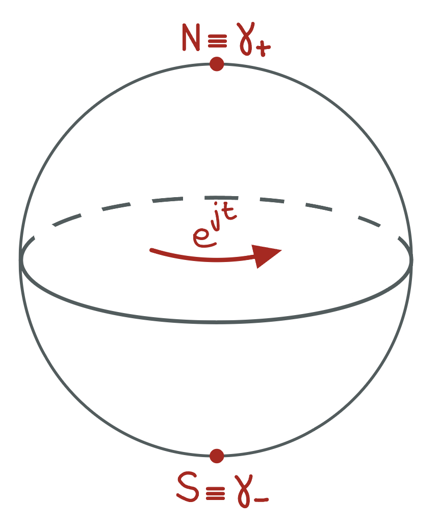
This description of the magnetic geodesics yields a nice visualization (Figure 1) in terms of the Hopf-fibration (for ). The factor is a rotation in the fibers, while the factor projects down to a rotation of with rotation axis determined by . Explicitly, the two fixed antipodal points of the rotation are the projections of solutions to the equation .
We can now prove that the only fast periodic magnetic geodesics on are the quotients of the Reeb orbits over the antipodal points .
Lemma 2.5.
All non-constant periodic magnetic geodesics on of period except for the Reeb orbits satisfy
Proof.
All magnetic geodesics on that lift to closed magnetic geodesic on satisfy the bound by Lemma 2.2. Therefor let be a magnetic geodesic of period on that satisfies
| (7) |
which is equivalent to projecting to a short magnetic geodesic on . As this implies that projects under the Hopf map to a rotation of that preserves the geodesic circle , which implies . Evaluating equation (7) at we find
where . Multiplying both entries yields which implies
unless or which are precisely the orbits . ∎
Step 2: Adding a potential – magnetic billiards
In order to construct an admissible Hamiltonian on (an open set of) we need to modify , so that all non-constant periodic orbits have period . Recall that are the only periodic orbits that will cause problems, so we will try to cut them out using a potential. Again we first construct the potential on and later argue that it descends to . If
denotes the Hopf-map with respect to , these two orbits project to antipodal points. We call them and . Now the rotation projects under to the rotation of fixing and (see Figure 1). We want to modify by adding a potential that only depends on the distance , goes to infinity near and is zero outside the neighborhood of .
Proposition 2.6.
All periodic orbits of on have period
Here refers to the maximal velocity along the periodic orbit. Observe that as the potential vanishes where the velocity is maximal.
Notation 2.7.
From now on we will use the term by abuse of notation as a term that tends to zero as , but is not necessarily of order .
The idea of proof is very geometric: If is a sequence of periodic orbits of , then the -limit of as is either a magnetic bounce orbit on the billiard table or an orbit trapped near the boundary of the billiard table . (For a precise definition we refer to Appendix B.) In particular, when the periods of are bounded uniformly in , their periods converge to the periods of the bounce orbits.
Lemma 2.8.
All periodic magnetic bounce orbits on have period
Proof.
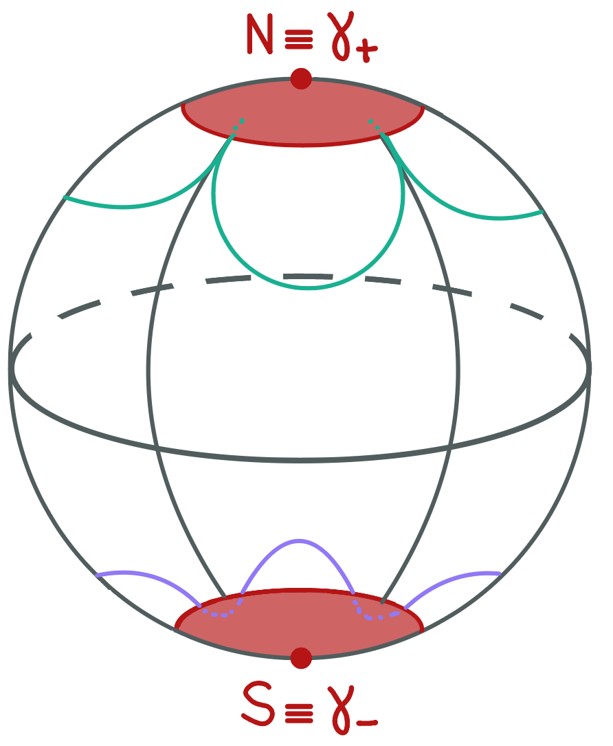
As shown in Figure 2 there are three types of bounce orbits. Type (1) is a smooth orbit and thus satisfies the period bound by Lemma 2.2. Type (2) bounces exactly at one of the poles. If it is periodic, its period is by symmetry the same as the orbit of the corresponding smooth orbit. Type (3) bounces at both poles and again using symmetries one can sees that its period is the same as the period of the corresponding smooth orbit. ∎
The detailed proof of Proposition 2.6 is written in Appendix B. It follows the strategy above arguing that for small any periodic orbit must either be close to a periodic bounce orbit or trapped near the poles. In the first case one obtains the bound from Lemma 2.8, in the second case from using some integrals of motion that are derived in Appendix A.
Remark 2.9.
The potential is -invariant, therefor the Hamiltonian descends to the lens space.
Corollary 2.10.
All periodic orbits of on have period
Proof.
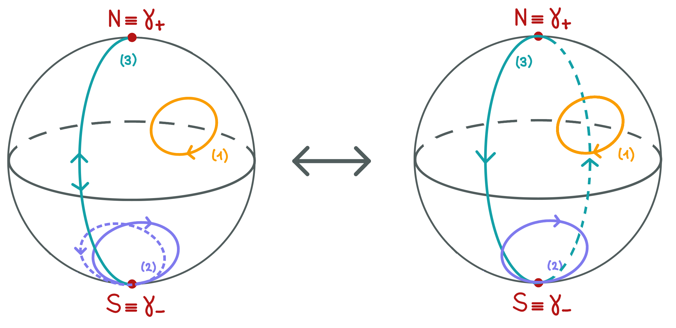
We need to check that -invariant orbits on have period at least times the above bound. A -invariant orbit is either a magnetic geodesic as in Lemma 2.5 and therefor its period satisfies Proposition 2.6 or it is a -symmetric configuration of magnetic geodesic arcs (see Figure 3). If it is not trapped near the caps this means it must have length tending to infinity as the bounce orbits are not -symmetric. If the orbit is trapped near a cap, it also must consists of at least magnetic geodesic arcs. This means it has winding number at least in Reeb direction and therefor on . ∎
Step 3: Constructing an admissible Hamiltonian
We can now reparametrize the magnetic billiard dynamics to write down a Hamiltonian with no fast periodic orbits.
Proposition 2.11.
We define the following Hamiltonian to reparametrize the dynamics induced by ,
where is given by
Then periodic orbits with respect to have periods
Remark 2.12.
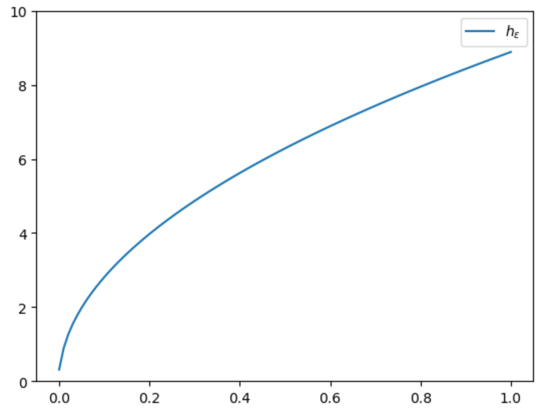
Note that is differentiable in particular at . The function is not smooth, i.e. of class , but one can approximate it by a smooth function, and as the period only sees the first derivative this will not change the bound on the period. In addition, for the reader’s convenience, we add an example of a possible graph of .
Proof.
Let be a periodic orbit of . There are two cases that we have to investigate. We start with . Using that for if , we find
Now if , recall that with . Thus we find
∎
We are finally in the position to prove the lower bound of the Hofer–Zehnder capacity.
Corollary 2.13.
The Hofer-Zehnder capacity is bounded from below by
where denotes the length of the shortest prime geodesics on .
Proof.
By monotonicity of capacities and using the shift of the zero-section (6) we find
Denote the sub level set of by
Observe that . Now we can modify
by composing it with another function
with , and , so that is admissible. Indeed the periods then satisfy
In particular, we obtain
Taking yields the corollary as the sphere covering the lens space was of radius and therefore its prime geodesic have length , while the shortest prime geodesics on have length . ∎
3 Upper bound: Capacity of
We will deduce the upper bound for disk tangent bundles of the lens spaces from the fact that they are all covered by the disk tangent bundle of the 3-sphere. To do so we first need to compute the Hofer–Zehnder capacity of .
Theorem 3.1.
Take the disk bundle with respect to the round metric and denote by the length of all prime geodesics, then
Proof.
We prove the Theorem by finding a lower and an upper bound that coincide. Further we normalize the metric such that , the general case follows by scaling.
Lower bound: All orbits of are periodic of period one. Composing the Hamiltonian with a suitable function we can extend smoothly to the zero-section such that is admissible and . Now the lower bound follows from .
Remark 3.2.
For the upper bound we will use results by Hofer–Viterbo [16] and Lu [20], using the theory of pseudoholomorphic curves or more precisely Gromov–Witten invariants to obtain an upper bound for the Hofer–Zehnder capacity. For a detailed introduction to Gromov-Witten invariants in symplectic topology we refer to [21]. We use the notation of Wendl [26] and denote by the count of pseudoholomorphic spheres representing the homology class with three marked points mapped to representatives of the homology classes .
Upper bound: As shown for example in [2, Lem. 3.2] the disk tangent bundle is symplectomorphic to the complement of 2-quadric in the 3-quadric, i.e.
Here and denotes the restriction of the Fubini-Study to normalized to take value on the generator of .
Note that is actually an irreducible Hermitian symmetric space of rank 2. By [19, Lem. 15] a Gromov–Witten invariant of the form for the generator of does not vanish. As by Lemma C.1 we have and therefor we find
Finally we can use a corollary [10, Cor. 3.2.11] of a theorem by Lu [20, Thm. 1.10] to find
∎
Remark 3.3.
Observe that is the generator of , therefor it is a minimal class and the moduli space of pseudoholomorphic curves in class is compact. The Gromov-Witten invariant we use here is thus defined without using any virtual techniques.
We can now deduce an upper bound for the Hofer–Zehnder capacity of .
Corollary 3.4.
The Hofer-Zehnder capacity is bounded from above by
where denotes the length of the shortest prime geodesics.
Proof.
Let be an admissible Hamiltonian, then is admissible for . In particular
as is the length of the prime geodesics on the sphere covering isometrically. ∎
4 Further directions
We will finish the article by discussing open problems which are in our opinion closely related to Theorem 1.3. The first question one has is probably, what about other lens spaces? First note that when considering lens spaces for even 2.1 does not hold, as every geodesic on covers a geodesic of at least twice. Still, as shown by the first author [9], for (e.g. ) Theorem 1.3 continues to hold. The lower bound in this case was obtained using geodesic billiards on one of the hemispheres of . For general odd the authors are optimistic that one could combine the two dynamics in order to find a lower bound. As the upper bound comes from it actually holds for any lens space .
Question 4.1.
Let co-prime and odd. Can one extend the proof of the lower bound in theorem 1.3 to compute the Hofer-Zehnder capacity ?
The guess of the authors would be yes, with the following modification one should instead of studying the magnetic flow equipped with it’s standard contact form the magnetic flow on the ellipsoid equipped with it’s standard contact form. This can be done as follows: we equip with the contact form . Note that the Reeb vector field is given by thus the Reeb flow w.r.t. on is given by . If we replace by again this Reeb flow can used to define a action on as follows
Dividing out this action on we obtain the Lens space .
Conjecture 4.2.
For all co-prime the Hofer-Zehnder capacity of the disk bundle of is given by
Lastly we also want to say a few words about higher dimensions. Again the upper bound continues to hold as also in higher dimensions, since we have
For the lower bound one could try to use the fact that the magnetic geodesic flow on actually stays on totally geodesic copies of which are invariant under the magnetic flow, see for reference [3]. Certainly the potential one uses can be extended to such that tends to infinity in a neighborhood of the Reeb orbits where is a rotation in the -th coordinate by the angle . So, we end up with the following:
Conjecture 4.3.
For all odd the Hofer-Zehnder capacity of the disk bundle of is given by
Appendix A Integrals of motion
We introduce the following coordinates on ,
for and . Observe that corresponds to and corresponds to and that
Hence, depends only on . The metric in these coordinates is
We plug into to obtain
Using that we can express the Lagrangian in coordinates
In particular, the Lagrangian does not depend on and . Therefore the conjugate momenta
| (8) |
are preserved. Since the kinetic energy is also an integral of motion the Lagrangian system has three independent integrals of motion. So the corresponding Hamiltonian system on is integrable, so we can conclude:
Corollary A.1.
The Hamiltonian system is integrable.
Appendix B Bound on periods
Let be a periodic orbit of . We consider the following cases.
As we added the potential , the norm of the velocity is not a constant of motion. However, every orbit leaves the region where the potential is non-vanishing and by conservation of energy the velocity is maximal there. From now on we denote the maximal velocity.
Avoids both caps: If avoids both caps it is a magnetic geodesic and therefor satisfies the bound in Lemma 2.2.
Trapped: The periodic orbit is ’trapped’ if it stays near the cap in the following sense
In coordinates this means either or . Both cases work analogously, so we only consider the case . As we immediately find
In particular as we have
If we could assume that , we could conclude
Indeed by the following argument. First, recall from [3] that if is a magnetic geodesic of strength , speed and enclose the angle with the Reeb vector field on , then the projection of onto for the Hopf fibration is a closed curve of radius
That might be surprising since one would expect that the radius of projections of magnetic geodesics only depends on the speed and the velocity. Now on the one hand we know that
as goes to zero. On the other hand if somewhere, it follows that . Using the energy bound we find
All together this implies
as . This contradicts and we conclude that .
Enters only one cap: If enters only one cap and is not trapped, we know that the magnetic geodesic it follows outside the caps is of (euclidean) radius . Denote the (euclidean) distance, between the center of the cap and the center of the magnetic geodesic and the radius of the cap. Now
thus using the estimates we find
We may assume to be small so that we can approximate to find
It follows that
This means as these orbits either approximate periodic bounce orbits of type (2) or have length tending to infinity. In particular
Enters both caps: Periodic orbits that enter both caps either approximate orbits of type (3) or their length tends to infinity as . In particular
Appendix C Cohomology of the quadric
The cohomology of is well known to experts, but for the sake of completeness, we add its computation in this article. The main tools are the Lefschetz hyperplane theorem and the Mayer-Vietoris sequence.
Lemma C.1.
The cohomology of the complex quadric is given by
Further the generators and have intersection equal to 1, i.e. .
Proof.
Using the direct corollaries [24, Cor. 1.24 & 1.25] of the Lefschetz hyperplane theorem for hypersurfaces, we immediately find for . To find one can for example apply the Mayer–Vietoris sequences to the decomposition where denotes the disk normal bundle of . Observe that , and as the tangent bundle of is trivializable. Therefor all terms but are known. The statement about the intersection again follows directly from [24, Cor. 1.25]. ∎
References
- [1] A. Abbondandolo, G. Benedetti, and O. Edtmair. Symplectic capacities of domains close to the ball and Banach–Mazur geodesics in the space of contact forms. arXiv preprint arxiv:2312.07363, 2023.
- [2] N. Adaloglou. Uniqueness of Lagrangians in . arXiv preprint arXiv:2201.09299, 2022.
- [3] P. Albers, G. Benedetti, and L. Maier. Magnetic geodesics on odd dimensional spheres. To appear.
- [4] P. Albers and M. Mazzucchelli. Periodic Bounce Orbits of Prescribed Energy. International Mathematics Research Notices, 2011(14):3289–3314, 01 2011.
- [5] S. Artstein-Avidan, R. Karasev, and Y. Ostrover. From symplectic measurements to the Mahler conjecture. Duke Math. J., 163(11), 2014.
- [6] G. Benedetti. The contact property for magnetic flows on surfaces. PhD Thesis, University of Cambridge, (see https://doi.org/10.17863/CAM.16235, or arXiv:1805.04916), 2014.
- [7] G. Benedetti, J. Bimmermann, and K. Zehmisch. Symplectic capacities of disc cotangent bundles of flat tori. arXiv preprint arXiv:2311.07351, 2023.
- [8] G. Benedetti and J. Kang. Relative Hofer–Zehnder capacity and positive symplectic homology. Journal of Fixed Point Theory and Applications, 24(2):44, 2022.
- [9] J. Bimmermann. Hofer-Zehnder capacity of disc tangent bundles of projective spaces. arXiv preprint arXiv:2306.11382, 2023.
- [10] J. Bimmermann. On the Hofer–Zehnder Capacity of Twisted Tangent Bundles. PhD thesis, 2023.
- [11] K. Cieliebak, H. Hofer, J. Latschev, and F. Schlenk. Quantitative symplectic geometry, page 1–44. Mathematical Sciences Research Institute Publications. Cambridge University Press, 2007.
- [12] D. Cristofaro-Gardiner and R. Hind. On the agreement of symplectic capacities in high dimension. arXiv preprint arxiv:2307.12125, 2023.
- [13] O. Edtmair. Disk-like surfaces of section and symplectic capacities. arXv preprint arxiv:2206.07847, 2023.
- [14] B. Ferreira and V. G. Ramos. Symplectic embeddings into disk cotangent bundles. Journal of Fixed Point Theory and Applications, 24(3):62, 2022.
- [15] J. Gutt, M. Hutchings, and V. G. B. Ramos. Examples around the strong Viterbo conjecture. Journal of Fixed Point Theory and Applications, 41, 2022.
- [16] H. Hofer and C. Viterbo. The Weinstein conjecture in the presence of holomorphic spheres. Communications on Pure and Applied Mathematics, 45(5):583–622, 1992.
- [17] H. Hofer and E. Zehnder. Symplectic invariants and Hamiltonian dynamics. Birkhäuser, 2011.
- [18] E. Lerman. Symplectic cuts. Math. Res. Lett., 2(3):247–258, 1995.
- [19] A. Loi, R. Mossa, and F. Zuddas. Symplectic capacities of Hermitian symmetric spaces. arXiv preprint arXiv:1302.1984, 2013.
- [20] G. Lu. Gromov-Witten invariants and pseudo symplectic capacities. Israel Journal of Mathematics, 156(1):1–63, 2006.
- [21] D. McDuff and D. Salamon. J-holomorphic curves and symplectic topology, volume 52. American Mathematical Soc., 2012.
- [22] M. Usher. Many closed symplectic manifolds have infinite Hofer–Zehnder capacity. Transactions of the American Mathematical Society, 364(11):5913–5943, 2012.
- [23] A.-M. Vocke. Periodic bounce orbits in magnetic billiard systems. PhD thesis, 2021.
- [24] C. Voisin. Hodge Theory and Complex Algebraic Geometry II: Volume 2, volume 77. Cambridge University Press, 2003.
- [25] J. Weber. Noncontractible periodic orbits in cotangent bundles and Floer homology. Duke Mathematical Journal, 133(3):527–566, 2006.
- [26] C. Wendl. Holomorphic curves in low dimensions. Springer, 2018.