One-Bit Target Detection in Collocated MIMO Radar with Colored Background Noise

Abstract

One-bit sampling has emerged as a promising technique in multiple-input multiple-output (MIMO) radar systems due to its ability to significantly reduce data volume and processing requirements. Nevertheless, current detection methods have not adequately addressed the impact of colored noise, which is frequently encountered in real scenarios. In this paper, we present a novel detection method that accounts for colored noise in MIMO radar systems. Specifically, we derive Rao’s test by computing the derivative of the likelihood function with respect to the target reflectivity parameter and the Fisher information matrix, resulting in a detector that takes the form of a weighted matched filter. To ensure the constant false alarm rate (CFAR) property, we also consider noise covariance uncertainty and examine its effect on the probability of false alarm. The detection probability is also studied analytically. Simulation results demonstrate that the proposed detector provides considerable performance gains in the presence of colored noise.

I Introduction

One-bit radar, characterized by the use of one-bit analog-to-digital converters (ADC), has witnessed significant advancements in radar processing and imaging domains in recent years [1, 2, 3, 4, 5, 6]. The primary advantage of one-bit sampling is its simplified hardware requirements and reduced power consumption, making it highly suitable for several applications, particularly on small platforms.

Although the sampling process potentially results in information loss, recent studies have demonstrated that this can be effectively mitigated through advanced signal processing techniques. In some instances, these methods can even enhance the overall system performance, for example, through a higher sampling rate [7]. Moreover, one-bit radar has proven capable of performing all the functions of traditional high-bit radar, including direction-of-arrival (DOA) estimation [8, 9, 10, 11], range and Doppler estimation [12, 13, 14, 15], detection [16, 17], tracking [18], and imaging [19, 20]. Consequently, one-bit radar is emerging as a important development direction in the radar field, with profound implications for the design and application of future radar systems, particularly in the context of efficient and accurate target detection.

However, most current research on one-bit radar operates under the assumption of white noise, which is often unrealistic in practice [21, 22, 23, 24, 25]. This discrepancy arises because, in the presence of colored noise, the likelihood function is described by central/non-central orthant probabilities, which lack closed-form expressions. Although these probabilities can be evaluated numerically using fast algorithms, they pose challenges for detection tasks since most detection criteria, such as the generalized likelihood ratio test (GLRT), are based on likelihood functions. Concretely, the orthant probabilities make it exceedingly difficult to determine the maximum likelihood estimate (MLE) of the target reflectivity parameter, thereby hindering the formulation of the GLRT. In this paper, we demonstrate that the derivative of the orthant probability with respect to the mean value can be expressed as an orthant probability of a lower dimension, which can also be numerically evaluated. Utilizing this property, we construct a Rao’s test [26, 28, 27] to address this problem, circumventing the need to compute the MLE.

It is important to note that Rao’s test does not need the MLE only in scenarios where the likelihood under the null is simple, which implies no unknown parameters [29]. Consequently, our detector’s development is based on the assumption that the noise covariance matrix is known. However, in practical applications, this matrix is often estimated from noise-only samples using, for instance, the algorithms described in [30, 31, 32, 33]. Hence, our subsequent analysis focuses on the impact of estimation errors on the detector’s performance. Initially, we explore how an increased false alarm rate can result from noise covariance mismatch. Specifically, we examine the detector’s distribution when the actual noise covariance matrix is assumed to be at a specific mismatched value. These results are then averaged, considering the prior distribution of estimation errors as provided in [30], using an improved Monte Carlo method. Employing this approach enables a more nuanced understanding of how estimation errors, characterized by the prior distribution, might influence the performance of the detector.

Continuing our analysis, we examine the detector’s detection performance and simplify the results to a non-central $\chi^{2}$ distribution. This simplification provides a clearer view of how noise covariance mismatch affects the detection process, particularly by reducing the non-centrality parameter. This reduction can be interpreted as a decrease in the “distance” between the null and non-null distributions, which provides valuable insights into the impact of covariance mismatch on the overall detection performance.

Finally, our theoretical findings are validated via computer simulations. It is shown that under realistic settings, the performance degradation due to noise covariance mismatch is almost negligible, especially when the number of noise-only samples is sufficient. This is a common scenario in one-bit processing, as the sampling rate can be significantly increased due to the simple structure of one-bit ADCs. Additionally, the simulation results confirm that the theoretical analysis accurately reflects the impact of noise mismatch on the null distribution, which allows us to adjust the threshold to maintain a constant false alarm rate (CFAR).

The contributions of this paper are summarized as:

1. Development of Rao’s Test for One-Bit Target Detection in Colored Noise: This paper extends our previous work on a white noise detector, as documented in [7]. To the best of our knowledge, this is the first study in the field of one-bit radar processing that takes into account colored noise. This advancement marks a significant step forward in enhancing the applicability and accuracy of one-bit radar systems.

2. Accurate Characterization of Null and Non-Null Distributions: We derive accurate expressions for the null and non-null distributions of the detector, which are crucial for accurately predicting the false alarm and detection probabilities. More importantly, they provide a deeper understanding of the detector’s behavior, aiding in a more informed and nuanced approach to radar detection challenges.

3. Analysis of Noise Covariance Matrix Mismatch Impact: We conduct an in-depth study of how discrepancies in the noise covariance matrix influence detection performance, including its impact on the null distribution. Our analysis reveals that the noise covariance matrix mismatch leads to an increased false alarm rate, necessitating adaptive threshold adjustments to preserve the CFAR property. Additionally, by approximating the non-null distribution by a non-central $\chi^{2}$ distribution, we show that performance degradation can be quantified as a decrease in the non-central parameter. This insight provides a clear and direct understanding of how noise covariance matrix mismatch affects system performance.

The remainder of this paper is organized as follows: Section II presents the signal model for one-bit detection in collocated MIMO radar under colored noise conditions. Section III details the derivation of a detector based on Rao’s test. The analysis of its null and non-null distributions is conducted in Sections IV and V, respectively, which also study the effect of noise mismatch. Section VI provides simulation results to corroborate the theoretical calculations. The paper concludes with a summary of the main findings.

Notation

Throughout this paper, we use boldface uppercase letters for matrices and boldface lowercase letters for column vectors, while lowercase letters denote scalar quantities. The notation $\mathbf{A}\in\mathbb{R}^{p\times q}\ (\mathbb{C}^{p\times q})$ indicates that $\mathbf{A}$ is a $p\times q$ real (complex) matrix. The $(i,j)-$th entry of $\mathbf{A}$ is denoted by $\mathbf{A}(i,j)$, and $\mathbf{a}(i)$ refers to the $i-$th entry of the vector $\mathbf{a}$. The trace of $\mathbf{A}$ is represented as $\text{tr}(\mathbf{A})$. The function ${\rm Diag}(\mathbf{A})$ retrieves the diagonal matrix of $\mathbf{A}$, and ${\rm diag}(\mathbf{a})$ produces a diagonal matrix with the elements of $\mathbf{a}$. The superscripts $(\cdot)^{-1}$, $(\cdot)^{T}$, and $(\cdot)^{H}$ represent the matrix inverse, transpose, and Hermitian transpose operators, respectively. The operators $\mathbb{E}[a]$ and $\mathbb{V}[a]$ denote the expected value and variance of $a$, respectively, while $\mathbb{C}[a,b]$ is the covariance between $a$ and $b$. The symbol $\sim$ means “distributed as”. The terms $\chi^{2}_{f}$ and $\chi^{2}_{f}(\delta^{2})$ refer, respectively, to the central and non-central Chi-squared distributions, where $f$ is the number of degrees of freedom (DOFs), and $\delta^{2}$ is the non-centrality parameter. Finally, the operators $\operatorname{Re}(\cdot)$ and $\operatorname{Im}(\cdot)$ extract the real and imaginary parts of their arguments, $\imath$ denotes the imaginary unit, and $\mathrm{sign}(\cdot)$ indicates the sign of its argument.

II Signal Model

We begin by examining a collocated MIMO radar setup, encompassing $p$ transmit and $m$ receive antennas. The transmit array emits a probing signal of length $n$, $\mathbf{S}\in\mathbb{C}^{p\times n}$, towards a specified angle $\phi$, which is then reflected by a far-field point source. The received signal at the input of the ADCs can be represented as:

$$\mathbf{X}=\begin{bmatrix}\mathbf{x}_{1},\cdots,\mathbf{x}_{n}\end{bmatrix}=\beta\mathbf{a}_{r}(\phi)\mathbf{a}_{t}^{T}(\phi)\mathbf{S}+\mathbf{N},$$ (1)

where $\beta$ is the target reflectivity, $\mathbf{a}_{t}(\phi)\in\mathbb{C}^{p\times 1}$ and $\mathbf{a}_{r}(\phi)\in\mathbb{C}^{m\times 1}$ are the transmit and receive steering vectors, respectively. The term $\mathbf{N}\in\mathbb{C}^{m\times n}$ denotes additive noise that is composed of $n$ independent and identically distributed Gaussian vectors with zero mean and covariance matrix $\boldsymbol{\Sigma}_{\mathbf{N}}$.

After one-bit quantization, the signal becomes

$$\mathbf{Y}=\begin{bmatrix}\mathbf{y}_{1},\cdots,\mathbf{y}_{n}\end{bmatrix}=\mathcal{Q}(\mathbf{X})=\mathrm{sign}(\mathrm{Re}(\mathbf{X}))+\imath\mathrm{sign}(\mathrm{Im}(\mathbf{X})),$$ (2)

where $\mathcal{Q}(\cdot)$ is the complex-valued quantization function.

Our objective is to detect the presence or absence of a target by analyzing the quantized observations $\mathbf{Y}$. Hypothesis $\mathcal{H}_{1}$ means that the target is present, while hypothesis $\mathcal{H}_{0}$ implies target absence. For the one bit measurements, the problem of target detection boils down to

$$\begin{array}[]{l}\mathcal{H}_{0}:\mathbf{Y}=\mathcal{Q}\left(\mathbf{N}\right),\\ \mathcal{H}_{1}:\mathbf{Y}=\mathcal{Q}\left(\beta\mathbf{W}+\mathbf{N}\right).\end{array}$$ (3)

that is, we test $\mathcal{H}_{0}:\beta=0$ vs. $\mathcal{H}_{0}:\beta\neq 0$. To simplify the derivation, we have include all known parameters into a single term, denoted as $\mathbf{W}=\mathbf{a}_{r}(\phi)\mathbf{a}_{t}^{T}(\phi)\mathbf{S}$.

Unlike the scenario discussed in [7], this paper delves into a more intricate yet commonly encountered situation where the noise is colored, implying that the covariance matrix $\boldsymbol{\Sigma}_{\mathbf{N}}$ deviates from being a diagonal matrix. Under such circumstances, the likelihood function is given by the non-central orthant probability, which is markedly more complex than the $Q$ function required in the case of white noise [7]. Consequently, there is a need to devise a new detector to address the case of colored noise, which we obtain under the following assumptions:

1. The columns of $\mathbf{N}$ are independently and identically distributed (i.i.d.) with a complex circular Gaussian distribution $\mathcal{CN}(\mathbf{0},\boldsymbol{\Sigma}_{\mathbf{N}})$.

2. The covariance matrix $\boldsymbol{\Sigma}_{\mathbf{N}}$ has been estimated using training data and is known to the receiver.

3. The parameter $\beta$ remains invariant throughout the entire observation period.

III Detector Design

Since the non-central orthant probability lacks a closed-form expression, standard criteria like the GLRT cannot be applied. Instead, we resort to numerical methods for constructing the detector. In this section, we demonstrate that the derivative of the orthant probability can be represented as a lower-dimensional orthant probability, which is computationally tractable. This insight leads us to formulate Rao’s test as a weighted sum of squared derivatives.

We start by stacking the real and imaginary parts of the received signal $\mathbf{x}_{i}$ as follows

$$\underline{\mathbf{x}}_{i}=\begin{bmatrix}\mathrm{Re}(\mathbf{x}_{i})\\ \mathrm{Im}(\mathbf{x}_{i})\end{bmatrix},$$ (4)

and similarly for $\mathbf{y}_{i}$

$$\underline{\mathbf{y}}_{i}=\begin{bmatrix}\mathrm{Re}(\mathbf{y}_{i})\\ \mathrm{Im}(\mathbf{y}_{i})\end{bmatrix}.$$ (5)

Given the circular nature of the noise, the covariance matrix of $\underline{\mathbf{x}}_{i}$ is

$${\boldsymbol{\Sigma}}_{\underline{\mathbf{x}}}=\frac{1}{2}\begin{bmatrix}\mathrm{Re}(\boldsymbol{\Sigma}_{\mathbf{N}})&-\mathrm{Im}(\boldsymbol{\Sigma}_{\mathbf{N}})\\ \mathrm{Im}(\boldsymbol{\Sigma}_{\mathbf{N}})&\mathrm{Re}(\boldsymbol{\Sigma}_{\mathbf{N}})\end{bmatrix}$$ (6)

Now, defining $\mathbf{w}_{i}=\mathbf{u}_{i}+\imath\mathbf{v}_{i}$, where $\mathbf{w}_{i}$ is the $i$th column of $\mathbf{W}$, and $\beta=a+\imath b$, the mean of $\underline{\mathbf{x}}_{i}$ is

$$\mathbb{E}[\underline{\mathbf{x}}_{i}]=\boldsymbol{\upsilon}_{i}=\begin{bmatrix}a\mathbf{u}_{i}-b\mathbf{v}_{i}\\ a\mathbf{v}_{i}+b\mathbf{u}_{i}\end{bmatrix}.$$ (7)

Additionally, the orthant probability is defined as

$$P(\boldsymbol{\mu},{\boldsymbol{\Sigma}})=\int_{0}^{\infty}\cdots\int_{0}^{\infty}\phi_{k}(\mathbf{x};\boldsymbol{\mu},{\boldsymbol{\Sigma}})\mathrm{d}x_{1}\ldots\mathrm{d}x_{k},$$ (8)

where $\phi_{k}(\mathbf{x};\boldsymbol{\mu},{\boldsymbol{\Sigma}})$ is the probability density function (PDF) of a $k$-dimensional Gaussian distribution $\mathcal{N}(\boldsymbol{\mu},\boldsymbol{\Sigma})$:

$$\phi_{k}(\mathbf{x};\boldsymbol{\mu},{\boldsymbol{\Sigma}})=\frac{1}{(2\pi)^{\frac{k}{2}}\left|\boldsymbol{\Sigma}\right|^{\frac{1}{2}}}\exp\left(-\frac{1}{2}(\mathbf{x}-\boldsymbol{\mu})^{T}\boldsymbol{\Sigma}^{-1}(\mathbf{x}-\boldsymbol{\mu})\right).$$ (9)

Based on these ingredients, and similar to [34], we can write the likelihood of the $i$th observation as

$$\mathcal{L}(\underline{\mathbf{y}}_{i};\boldsymbol{\theta})=\Pr\{\underline{\mathbf{y}}_{i};\boldsymbol{\theta}\}=\Pr\{\mathbf{Z}_{i}\underline{\mathbf{x}}_{i}\succ\mathbf{0};\boldsymbol{\theta}\}=P\left(\boldsymbol{\mu}_{i},\mathbf{C}_{i}\right),$$ (10)

where $\boldsymbol{\theta}=[a,b]^{T}$ is the vector representation of the unknown reflectivity $\beta$, $\mathbf{Z}_{i}={\rm diag}(\underline{\mathbf{y}}_{i})$, $\succ$ is the element-wise greater operator, and $P\left(\boldsymbol{\mu}_{i},\mathbf{C}_{i}\right)$ is the orthant probability with mean $\boldsymbol{\mu}_{i}=\mathbf{Z}_{i}\boldsymbol{\nu}_{i}$ and covariance matrix $\mathbf{C}_{i}=\mathbf{Z}_{i}\mathbf{C}\mathbf{Z}_{i}$, with $\boldsymbol{\nu}_{i}=\mathbf{D}^{-\frac{1}{2}}\boldsymbol{\upsilon}_{i},\mathbf{D}={\rm Diag}({\boldsymbol{\Sigma}}_{\underline{\mathbf{x}}})$, and $\mathbf{C}=\mathbf{D}^{-\frac{1}{2}}{\boldsymbol{\Sigma}}_{\underline{\mathbf{x}}}\mathbf{D}^{-\frac{1}{2}}$ is a coherence matrix [37]. Note that the means $\boldsymbol{\mu}_{i}$ depend on $\boldsymbol{\theta}$ (through $\boldsymbol{\upsilon}_{i}$), but the covariance matrices $\mathbf{C}_{i}$ do not. Taking the independence between the samples into account, we can obtain the log-likelihood function under $\mathcal{H}_{1}$ as

$$\mathcal{L}(\mathbf{Y};\boldsymbol{\theta})=\sum_{i=1}^{n}\mathcal{L}(\underline{\mathbf{y}}_{i};\boldsymbol{\theta})=\sum_{i=1}^{n}\log P(\boldsymbol{\mu}_{i},\mathbf{C}_{i}),$$ (11)

and by noting that under $\mathcal{H}_{0}$, $\boldsymbol{\theta}=\boldsymbol{\theta}_{0}=[0,0]^{T}$, the log-likelihood function becomes

$$\mathcal{L}(\mathbf{Y};\boldsymbol{\theta}_{0})=\sum_{i=1}^{n}\log P(\mathbf{0}_{2m},\mathbf{C}_{i}),$$ (12)

which depends only on the known covariance matrices.

Since there are no unknown parameters under $\mathcal{H}_{0}$, we propose to use Rao’s test to address this problem, given by

$$T_{\text{R}}=\left(\!\left.\frac{\partial\mathcal{L}(\mathbf{Y};\boldsymbol{\theta})}{\partial\boldsymbol{\theta}}\right|_{\boldsymbol{\theta}=\boldsymbol{\theta}_{0}}\!\right)^{T}\!\!\mathbf{F}^{-1}\!\!\left(\!\boldsymbol{\theta}_{0}\right)\left(\left.\frac{\partial\mathcal{L}(\mathbf{Y};\boldsymbol{\theta})}{\partial\boldsymbol{\theta}}\right|_{\boldsymbol{\theta}=\boldsymbol{\theta}_{0}}\!\right),$$ (13)

where $\mathbf{F}\left(\!\boldsymbol{\theta}\right)$ is the Fisher information matrix (FIM)

$$\mathbf{F}\left(\!\boldsymbol{\theta}\right)=\mathbb{E}\left[\frac{\partial\mathcal{L}(\mathbf{Y};\boldsymbol{\theta})}{\partial\boldsymbol{\theta}}\frac{\partial\mathcal{L}(\mathbf{Y};\boldsymbol{\theta})}{\partial\boldsymbol{\theta}^{T}}\right].$$ (14)

Denoting $P_{i}=P(\boldsymbol{\mu}_{i},\mathbf{C}_{i})$, the derivatives are

$$\frac{\partial\mathcal{L}}{\partial a}= \sum_{i=1}^{n}\frac{1}{P_{i}}\frac{\partial P_{i}}{\partial a}=\sum_{i=1}^{n}\sum_{j=1}^{2m}\frac{1}{P_{i}}\frac{\partial P_{i}}{\partial\boldsymbol{\mu}_{i}(j)}\frac{\partial\boldsymbol{\mu}_{i}(j)}{\partial a}$$ (15a)

$$\frac{\partial\mathcal{L}}{\partial b}= \sum_{i=1}^{n}\frac{1}{P_{i}}\frac{\partial P_{i}}{\partial b}=\sum_{i=1}^{n}\sum_{j=1}^{2m}\frac{1}{P_{i}}\frac{\partial P_{i}}{\partial\boldsymbol{\mu}_{i}(j)}\frac{\partial\boldsymbol{\mu}_{i}(j)}{\partial b},$$ (15b)

where the right-most derivatives are

$$\frac{\partial\boldsymbol{\mu}_{i}}{\partial a} =\mathbf{Z}_{i}\mathbf{D}^{-\frac{1}{2}}\begin{bmatrix}\mathbf{u}_{i}\\ \mathbf{v}_{i}\end{bmatrix}=\mathbf{Z}_{i}\mathbf{a}_{i}$$ (16a)

$$\frac{\partial\boldsymbol{\mu}_{i}}{\partial b} =\mathbf{Z}_{i}\mathbf{D}^{-\frac{1}{2}}\begin{bmatrix}-\mathbf{v}_{i}\\ \mathbf{u}_{i}\end{bmatrix}=\mathbf{Z}_{i}\mathbf{b}_{i}.$$ (16b)

To compute the derivative of the orthant probability with respect to the mean values, we introduce the following lemma.

Lemma 1

For an orthant probability $P(\boldsymbol{\mu},{\boldsymbol{\Sigma}})$, the derivative with respect to the $j$th element of $\boldsymbol{\mu}$ is

$$\frac{\partial P(\boldsymbol{\mu},{\boldsymbol{\Sigma}})}{\partial\boldsymbol{\mu}(j)}=\frac{1}{\sqrt{2\pi\boldsymbol{\Sigma}(j,j)}}P(\boldsymbol{\omega}(\boldsymbol{\mu},j),\mathbf{R}(\boldsymbol{\Sigma},j)),$$ (17)

where $\boldsymbol{\omega}(\boldsymbol{\mu},j)$ denotes the reduced vector after removing the $j$th element of $\boldsymbol{\mu}$ and

$$\mathbf{R}(\boldsymbol{\Sigma},j)=\boldsymbol{\Theta}(\boldsymbol{\Sigma},j)-\frac{1}{\boldsymbol{\Sigma}(j,j)}\mathbf{r}_{j}\mathbf{r}_{j}^{T},$$ (18)

where $\boldsymbol{\Theta}(\boldsymbol{\Sigma},j)$ denotes the reduced matrix after removing the $j$th row and column of $\boldsymbol{\Sigma}$, $\boldsymbol{\Sigma}(i,j)$ is the $(i,j)$th element of $\boldsymbol{\Sigma}$ and $\mathbf{r}_{j}$ is the reduced vector after removing the $j$th element of the $j$th column of $\boldsymbol{\Sigma}$.

Proof:

See Appendix A. ∎

This lemma has shown that when computing the derivative of the orthant probability of a $k$-dimensional Gaussian vector, we need to compute the orthant probability of a $(k-1)$-dimensional Gaussian vector. Now, Lemma 1 allows us to write

$$\left.\frac{\partial P_{i}}{\partial\boldsymbol{\mu}_{i}(j)}\right|_{\boldsymbol{\theta}=\mathbf{0}}=\frac{1}{\sqrt{2\pi}}P(\mathbf{0},\mathbf{R}(\mathbf{C}_{i},j)),$$ (19)

and the derivatives in (15) become

$$\left.\frac{\partial\mathcal{L}}{\partial\boldsymbol{\theta}}\right|_{\boldsymbol{\theta}=\mathbf{0}}=\begin{bmatrix}\displaystyle\frac{\partial\mathcal{L}}{\partial a}&\displaystyle\frac{\partial\mathcal{L}}{\partial b}\end{bmatrix}^{T}=\begin{bmatrix}\text{tr}(\mathbf{A}^{T}\mathbf{L}\mathbf{P}^{-1})\\ \text{tr}(\mathbf{B}^{T}\mathbf{L}\mathbf{P}^{-1})\end{bmatrix},$$ (20)

where

$$\mathbf{A} =[\mathbf{a}_{1},\cdots,\mathbf{a}_{n}], \mathbf{B} =[\mathbf{b}_{1},\cdots,\mathbf{b}_{n}],$$ (21)

and

$$\mathbf{P} ={\rm diag}(P(\mathbf{0}_{2m},\mathbf{C}_{1}),\cdots,P(\mathbf{0}_{2m},\mathbf{C}_{n})),$$ (22)

$$\mathbf{L} =\left[\mathbf{Z}_{1}\left.\frac{\partial P_{1}}{\partial\boldsymbol{\mu}_{1}}\right|_{\boldsymbol{\theta}=\mathbf{0}},\cdots,\left.\mathbf{Z}_{n}\frac{\partial P_{n}}{\partial\boldsymbol{\mu}_{n}}\right|_{\boldsymbol{\theta}=\mathbf{0}}\right],$$ (23)

where

$$\left.\frac{\partial P_{i}}{\partial\boldsymbol{\mu}_{i}}\right|_{\boldsymbol{\theta}=\mathbf{0}}\!=\frac{1}{\sqrt{2\pi}}\begin{bmatrix}P(\mathbf{0},\mathbf{R}(\mathbf{C}_{i},1)),\cdots,P(\mathbf{0},\mathbf{R}(\mathbf{C}_{i},2m))\end{bmatrix}^{T}\!.$$ (24)

In addition, Appendix B shows that the FIM is

$$\mathbf{F}(\boldsymbol{\theta}_{0})=\upsilon^{2}\mathbf{I}_{2},$$ (25)

where

$$\upsilon^{2}=\text{tr}\left(\boldsymbol{\Delta}_{1}^{T}\boldsymbol{\Delta}_{1}\mathbf{O}^{-1}\right)=\text{tr}\left(\boldsymbol{\Delta}_{2}^{T}\boldsymbol{\Delta}_{2}\mathbf{O}^{-1}\right),$$ (26)

with $\mathbf{O}$ defined in (92), and $\boldsymbol{\Delta}_{1}$ and $\boldsymbol{\Delta}_{2}$ defined in (93).

As a result, Rao’s test is formulated as:

$$T_{\rm R}=\frac{1}{\upsilon^{2}}\Big{[}\text{tr}^{2}(\mathbf{A}^{T}\mathbf{L}\mathbf{P}^{-1})+\text{tr}^{2}(\mathbf{B}^{T}\mathbf{L}\mathbf{P}^{-1})\Big{]}\mathop{\gtrless}\limits_{\mathcal{H}_{0}}^{\mathcal{H}_{1}}\gamma.$$ (27)

Combining (27) with (23) and (21), it becomes clear that the detector can be interpreted as a weighted matched filter. The weights for this filter are calculated using orthant probabilities and their derivatives, which are determined by the elements of the noise covariance matrix.

Remark 1

For each detection process, it becomes evident that we must calculate $2^{2m}$ orthant probabilities of dimension $2m$ for constructing $\mathbf{O}$, some of which are also necessary to construct $\mathbf{P}$. Notably, if every element of a given sample vector undergoes bit-wise inversion, the orthant probability associated with this modified vector remains identical to that of the original sample. This symmetry allows us to halve the number of necessary orthant probability calculations to $2^{2m-1}$. Furthermore, we must consider situations where some sample vectors corresponding to these probabilities might not be observed in the data. Consequently, the maximum number of orthant probabilities requiring evaluation is limited to $\min(2^{2m-1},n)$. Regarding the derivatives, our computations involve $n$ orthant probabilities of dimension $2m-1$, some of which can be identical for identical observations. Taking into account the previous symmetry, the number of computations required for the derivatives is $\min(2^{2m-2},\tilde{n})$, if there are $\tilde{n}\,(\leq n)$ distinct observations.

Several efficient algorithms for evaluating orthant probabilities exist in the literature [35, 36]. Leveraging these advanced methodologies significantly reduces the computational burden involved in the detector construction, thereby facilitating practical, real-world applications.

IV Null distribution

In this section, we delve into the null distribution of the proposed detector $T_{\rm R}$. Initially, we consider the scenario with perfectly known noise covariance matrix. Subsequently, we analyze the effect on the false alarm rate when the noise covariance matrix is known up to some estimation error. Our study employs an improved Monte Carlo approach, which begins with a distribution for a specific error matrix. We then compute the average effect over the prior distribution of this error matrix via Monte Carlo, leading to the null distribution for the scenario of imperfect noise covariance matrix estimation.

IV-A Distribution with Known Noise Covariance

Let us start by rewriting the test statistic as

$$T_{\text{R}}=w_{1}^{2}+w_{2}^{2},$$ (28)

where

$$w_{1} =\frac{1}{\upsilon}\text{tr}(\mathbf{A}^{T}\mathbf{L}\mathbf{P}^{-1}), w_{2} =\frac{1}{\upsilon}\text{tr}(\mathbf{B}^{T}\mathbf{L}\mathbf{P}^{-1}).$$ (29)

Since that the samples are i.i.d. under $\mathcal{H}_{0}$, it follows straightforwardly from the central limit theorem that $w_{1}$ and $w_{2}$ follow asymptotically ($n\rightarrow\infty$) a $2$-dimensional joint Gaussian distribution. In addition, recalling that

$$\mathbf{w}=[w_{1},w_{2}]^{T}=\frac{1}{\upsilon}\left[\frac{\partial\mathcal{L}(\mathbf{Y};\boldsymbol{\theta})}{\partial a},\frac{\partial\mathcal{L}(\mathbf{Y};\boldsymbol{\theta})}{\partial b}\right]^{T},$$ (30)

and taking (25) into account, it is easy to show that

$$\mathbb{E}[\mathbf{w}] =\mathbf{0}_{2}, \mathbb{E}[\mathbf{w}\mathbf{w}^{T}] =\mathbf{I}_{2},$$ (31)

which allows us to conclude that $T_{\text{R}}$ is asymptotically ($n\rightarrow\infty$) Chi-square distributed with 2 degrees of freedom (DoFs),

$$T_{\text{R}}\sim\chi^{2}_{2}.$$ (32)

That is, $T_{\text{R}}$ is exponentially distributed with parameter $1/2$, the probability of false alarm becomes

$$P_{\rm fa}(\gamma)=\text{Pr}\{T_{\text{R}}>\gamma\}=\exp(-\gamma/2),$$ (33)

and the detection threshold can be obtained as

$$\gamma=-2\log(P_{\rm fa}).$$ (34)

IV-B Distribution with Estimated Noise Covariance

In the preceding derivations, the noise covariance matrix was assumed to be perfectly known to the receiver. However, in reality, it must be estimated using, for instance, the algorithms in [30, 31, 32]. Accordingly, we need to account for the mismatch between the true and estimated noise covariance matrices and assess its impact. In this subsection, the scenario where the estimated covariance matrix, $\boldsymbol{\Sigma}_{\underline{\mathbf{x}}}$, and the true covariance matrix, $\boldsymbol{\Sigma}^{\prime}_{\underline{\mathbf{x}}}$, differ is examined, aiming to study the changes of the null distribution. We proceed with two assumptions: 1) the true covariance matrix $\boldsymbol{\Sigma}^{\prime}_{\underline{\mathbf{x}}}$ is close to the estimate $\boldsymbol{\Sigma}_{\underline{\mathbf{x}}}$, a condition that can be ensured by a sufficient amount of (training) samples, and 2) the prior distribution of $\boldsymbol{\Sigma}^{\prime}_{\underline{\mathbf{x}}}$ given $\boldsymbol{\Sigma}_{\underline{\mathbf{x}}}$ is known, which was obtained in [30].

We start by analyzing the joint distribution of $w_{1}$ and $w_{2}$ for the estimated covariance matrix, which is given by the following theorem.

Theorem 1

Under noise covariance mismatch, the distribution of $\mathbf{w}=[w_{1},w_{2}]^{T}$ can be asymptotically ($n\rightarrow\infty$) approximated by the real Gaussian distribution with zero mean and covariance matrix

$$\boldsymbol{\Sigma}_{w}=\mathbb{E}[\mathbf{w}\mathbf{w}^{T}]=\upsilon^{2}_{1}\mathbf{I}_{2},$$ (35)

where

$$\upsilon^{2}_{1}=\text{tr}\left(\boldsymbol{\Delta}_{1}^{T}\boldsymbol{\Delta}_{1}\mathbf{G}\right)=\text{tr}\left(\boldsymbol{\Delta}_{2}^{T}\boldsymbol{\Delta}_{2}\mathbf{G}\right),$$ (36)

with

$$\mathbf{G}={\rm diag}\left(\frac{O_{1}^{\prime}}{O_{1}^{2}},\cdots,\frac{O_{\kappa}^{\prime}}{O_{\kappa}^{2}}\right),$$ (37)

and $O^{\prime}_{1},\cdots,O^{\prime}_{\kappa}$ are defined in (95).

Proof:

See Appendix C. ∎

Using Theorem 1, we have

$$\frac{{\upsilon^{2}}}{\upsilon^{2}_{1}}T_{\text{R}}\sim\chi^{2}_{2}.$$ (38)

Therefore, the probability of false alarm can be rewritten as

$$P_{\rm fa}(\gamma)=\exp\left(-\frac{\upsilon^{2}}{2\upsilon^{2}_{1}}\gamma\right),$$ (39)

and the detection threshold is

$$\gamma=-\frac{2\upsilon^{2}_{1}}{\upsilon^{2}}\log(P_{\rm fa}).$$ (40)

IV-C Average over Prior Distribution of Estimation Error

In practical scenarios, the receiver typically does not know the estimation error of the noise covariance matrix. Instead, this error is characterized by a prior distribution, which can be derived using analytical methods detailed in the literature, such as [30]. Assuming that $\boldsymbol{\Sigma}^{\prime}_{\underline{\mathbf{x}}}$ has a known prior PDF given by $f(\boldsymbol{\Sigma}^{\prime}_{\underline{\mathbf{x}}})$, the probability of false alarm can be computed as

$$P_{\rm fa}(\gamma) =\int\text{Pr}\{T_{\text{R}}>\gamma|\boldsymbol{\Sigma}^{\prime}_{\underline{\mathbf{x}}}\}f(\boldsymbol{\Sigma}^{\prime}_{\underline{\mathbf{x}}})\mathrm{d}\boldsymbol{\Sigma}^{\prime}_{\underline{\mathbf{x}}}$$

$$=\int\exp\left(-\frac{\upsilon^{2}}{2\upsilon^{2}_{1}}\gamma\right)f(\boldsymbol{\Sigma}^{\prime}_{\underline{\mathbf{x}}})\mathrm{d}\boldsymbol{\Sigma}^{\prime}_{\underline{\mathbf{x}}}.$$ (41)

Given that evaluating $\upsilon^{2}_{1}$ for each $\boldsymbol{\Sigma}^{\prime}_{\underline{\mathbf{x}}}$ involves computing $2^{2m}$ orthant probabilities, which do not have a closed-form, computing this integral directly is very challenging. To avoid this, we present an improved Monte Carlo method to approximate (41). Concretely, we generate a sequence of $N$ covariance matrices from the prior distribution $f(\boldsymbol{\Sigma}^{\prime}_{\underline{\mathbf{x}}})$ and approximate the false alarm probability by averaging the outcomes as

$$P_{\rm fa}(\gamma)\approx\frac{1}{N}\sum_{i=1}^{N}\exp\left(-\frac{\upsilon^{2}}{2\upsilon^{2}_{1,i}}\gamma\right),$$ (42)

where $\upsilon^{2}_{1,i}=\text{tr}(\boldsymbol{\Delta}_{1}^{T}\boldsymbol{\Delta}_{1}\mathbf{G}_{i})=\text{tr}(\boldsymbol{\Delta}_{2}^{T}\boldsymbol{\Delta}_{2}\mathbf{G}_{i})$, where

$$\mathbf{G}_{i}={\rm diag}\left(\frac{O_{1,i}^{\prime}}{O_{1}^{2}},\cdots,\frac{O_{\kappa,i}^{\prime}}{O_{\kappa}^{2}}\right),$$ (43)

and $O^{\prime}_{j,i}=P(\mathbf{0},{\boldsymbol{\Gamma}}_{j}\mathbf{C}_{i}^{\prime}{\boldsymbol{\Gamma}}_{j})$, with $\mathbf{C}_{i}$ being the coherence matrix of $\boldsymbol{\Sigma}^{\prime}_{\underline{\mathbf{x}_{i}}}$, which is the $i$th covariance matrix drawn from the prior distribution.

Achieving an accurate approximation requires a large $N$, which in turn increases computational complexity since we have to compute $\upsilon^{2}_{1,i},i=1,\ldots,N$, which requires the computation of $2^{2m}$ orthant probabilities. However, we can optimize the process using a Taylor’s expansion around $\mathbf{C}_{0}$, which is the coherence matrix of the estimated noise covariance matrix, $\boldsymbol{\Sigma}_{\underline{\mathbf{x}}}$, to compute the orthant probabilities required for $\upsilon^{2}_{1}$ for each $\boldsymbol{\Sigma}^{\prime}_{\underline{\mathbf{x}}_{i}}$. The orthant probability can be approximated as

$$P(\mathbf{0}_{2m},{\mathbf{C}}_{i})\approx P(\mathbf{0}_{2m},{\mathbf{C}}_{0})+\left.\frac{\partial P(\mathbf{0}_{2m},\mathbf{C})}{\partial\mathbf{c}}\right|_{\mathbf{c}=\mathbf{c}_{0}}(\mathbf{c}_{0}-\mathbf{c}_{i}),$$ (44)

where $\mathbf{c}=\mathop{\text{vech}}(\mathbf{C})=[\mathbf{C}(1,2),\cdots,\mathbf{C}(2m-1,2m)]^{T}$ is the half vectorization of $\mathbf{C}$ without the main diagonal, that is, its upper triangular part, and comprises the free parameters of $\mathbf{C}$. Moreover, $\mathbf{c}_{0}=\mathop{\text{vech}}(\mathbf{C}_{0})$ and $\mathbf{c}_{i}=\mathop{\text{vech}}(\mathbf{C}_{i})$. The partial derivative in this expression can be efficiently computed using the following theorem.

Theorem 2

The derivative of the orthant probability $P(\mathbf{0}_{k},\mathbf{C})$ with respect to the correlation coefficient $\mathbf{C}(r,s)$, $r<s,$ is

$$\frac{\partial P(\mathbf{0}_{2m},\mathbf{C})}{\partial\mathbf{C}(r,s)}=\frac{P(\mathbf{0}_{k-2},\tilde{\mathbf{C}})}{2\pi\sqrt{1-|\mathbf{C}(r,s)|^{2}}},$$ (45)

where $\tilde{\mathbf{C}}=[\boldsymbol{\Theta}(\boldsymbol{\Theta}(\mathbf{C}^{-1},r),s-1)]^{-1}$.

Proof:

See Appendix D. ∎

Using this approach, we can avoid computing the orthant probability for each generated $\boldsymbol{\Sigma}^{\prime}_{\underline{\mathbf{x}}_{i}}$. Instead, we only need to compute derivative and can then generate a large number of $\boldsymbol{\Sigma}^{\prime}_{\underline{\mathbf{x}}_{i}}$ to obtain a reliable approximation to the null distribution. Let us start by writing

$$\upsilon^{2}_{1,i}=\upsilon^{2}+\upsilon^{2}_{\bigtriangleup,i},$$ (46)

where

$$\upsilon^{2}_{\bigtriangleup,i}=\text{tr}\left(\boldsymbol{\Delta}_{1}^{T}\boldsymbol{\Delta}_{1}(\mathbf{G}_{i}-\mathbf{O}^{-1})\right)=\text{tr}\left(\boldsymbol{\Delta}_{2}^{T}\boldsymbol{\Delta}_{2}(\mathbf{G}_{i}-\mathbf{O}^{-1})\right),$$ (47)

with

$$\mathbf{G}_{i}-\mathbf{O}^{-1}={\rm diag}\left(\frac{\Delta O_{1,i}}{O_{1}^{2}},\cdots,\frac{\Delta O_{\kappa,i}}{O_{\kappa}^{2}}\right).$$ (48)

In this expression, $\Delta O_{j,i}=O^{\prime}_{j,i}-O_{j}$ can be approximated using (44) as

$$\Delta O_{j,i}=\left.\frac{\partial P(\mathbf{0}_{2m},\mathbf{C})}{\partial\mathbf{c}}\right|_{\mathbf{c}=\tilde{\mathbf{c}}_{j,0}}(\tilde{\mathbf{c}}_{j,0}-\tilde{\mathbf{c}}_{j,i}).$$ (49)

where $\tilde{\mathbf{c}}_{j,0}=\mathop{\text{vech}}(\boldsymbol{\Gamma}_{j}\mathbf{C}_{0}\boldsymbol{\Gamma}_{j})$ and $\tilde{\mathbf{c}}_{j,i}=\mathop{\text{vech}}(\boldsymbol{\Gamma}_{j}\mathbf{C}_{i}\boldsymbol{\Gamma}_{j})$. From this expression, it can be seen that orthant probabilities are computed only for $\mathbf{C}_{0}$ and not for the $N$ realizations of $\boldsymbol{\Sigma}^{\prime}_{\underline{\mathbf{x}}_{i}}$. Finally, substituting (46) into (39), the average probability of false alarm can be estimated as

$$P_{\rm fa}(\gamma)\approx\frac{1}{N}\sum_{i=1}^{N}\exp\left(-\frac{\upsilon^{2}}{2\left(\upsilon^{2}+\upsilon^{2}_{\bigtriangleup_{i}}\right)}\gamma\right).$$ (50)

V Non-null distribution

In this section, the non-null distribution of the proposed detector is examined. Initially, a generalized non-central $\chi^{2}$ distribution is introduced through the analysis of the joint distribution of $w_{1}$ and $w_{2}$. Subsequently, a simplified representation is derived for the low signal-to-noise ratio (SNR) scenario using a Taylor’s expansion, yielding a standard non-central $\chi^{2}$ distribution.

V-A Fundamental Result

Let us start by computing the mean and covariance matrix of $\mathbf{w}$ under $\mathcal{H}_{1}$, which are presented in the following theorem.

Theorem 3

Under $\mathcal{H}_{1}$, the mean and covariance matrix of $\mathbf{w}$ are

$$\mathbf{u}_{w}(\beta) =\frac{1}{\upsilon}\begin{bmatrix}\text{tr}(\mathbf{G}_{1}\mathbf{Q}^{T})\\ \text{tr}(\mathbf{G}_{2}\mathbf{Q}^{T})\end{bmatrix}, \boldsymbol{\Sigma}_{w}(\beta) =\begin{bmatrix}\sigma_{1}^{2}&\sigma_{12}\\ \sigma_{12}&\sigma_{2}^{2}\end{bmatrix},$$ (51)

where $\mathbf{G}_{l}=\boldsymbol{\Delta}_{l}\mathbf{O}^{-1},l=1,2,$ and $\mathbf{Q}(i,j)=P({\boldsymbol{\Gamma}}_{j}\boldsymbol{\nu}_{i},{\boldsymbol{\Gamma}}_{j}\mathbf{C}{\boldsymbol{\Gamma}}_{j}),i=1,\dots,n,j=1,\ldots,\kappa$. The elements of the covariance matrix are given in Appendix E.

Having obtained the mean and covariance matrix of $\mathbf{w}$ under $\mathcal{H}_{1}$, we now define

$$\boldsymbol{\Sigma}_{w} =\mathbf{P}^{T}\boldsymbol{\Lambda}\mathbf{P}, \mathbf{m} =\mathbf{P}\boldsymbol{\Sigma}_{w}^{-\frac{1}{2}}\mathbf{u}_{w}.$$ (52)

Then, as in [7], the detector can be rewritten as

$$T_{\text{R}}=\lambda_{1}(\nu_{1}+m_{1})^{2}+\lambda_{2}(\nu_{2}+m_{2})^{2},$$ (53)

where $\boldsymbol{\Lambda}={\rm diag}(\lambda_{1},\lambda_{2})$, $\mathbf{m}=[m_{1},m_{2}]^{T}$, and $\nu_{1}$, $\nu_{2}$ are mutually independent standard Gaussian random variables. Thus, the detection probability of $T_{\text{R}}$ is given by a general non-central $\chi^{2}$ distribution:

$$T_{\text{R}}=\sum_{l=1}^{2}\lambda_{l}\chi^{2}_{1}(m_{l}^{2}),$$ (54)

which can be numerically evaluated [38].

It is easily proved that in the case of a mismatched noise covariance matrix, the result is adjusted by substituting $\mathbf{Q}$ with $\mathbf{Q}^{\prime}$, which is defined as follows:

$$\mathbf{Q}^{\prime}(i,j)=P({\boldsymbol{\Gamma}}_{j}\mathbf{s}^{\prime}_{i},{\boldsymbol{\Gamma}}_{j}\mathbf{C}^{\prime}{\boldsymbol{\Gamma}}_{j}),$$ (55)

Here, $\mathbf{C}^{\prime}$ represents the correlation matrix corresponding to the mismatched covariance matrix ${\boldsymbol{\Sigma}}^{\prime}_{\underline{\mathbf{x}}}$. Simultaneously, $\mathbf{s}^{\prime}_{i}={\rm diag}({\boldsymbol{\Sigma}}^{\prime}_{\underline{\mathbf{x}}})^{-\frac{1}{2}}\boldsymbol{\upsilon}_{i}$ characterizes the changes in the mean due to the covariance mismatch.

V-B Low-SNR Approximation

Despite its near-exact nature, the aforementioned approximation requires the computation of the orthant probability for all $n$ samples. In this sub-section, a simplified approximation is presented for the low-SNR regime via a Taylor’s approximation, which avoids additional orthant probability computations. The derived result is presented in the following theorem.

Theorem 4

In the low-SNR regime where $|\beta|=\mathcal{O}(n^{-\frac{1}{2}})$, the mean and covariance matrix of vector $\mathbf{w}$ for the matched noise covariance case are:

$$\mathbf{u}_{w} =\upsilon\begin{bmatrix}a\\ b\end{bmatrix}+\mathcal{O}(n^{-\frac{1}{2}}), \boldsymbol{\Sigma}_{\mathbf{w}} =\mathbf{I}_{2}+\mathcal{O}(n^{-\frac{1}{2}}).$$ (56)

Furthermore, for the mismatched noise covariance case, they becomes as:

$$\mathbf{u}_{w} =\frac{1}{\upsilon}\begin{bmatrix}a\varsigma^{2}_{1}\\ b\varsigma^{2}_{2}\end{bmatrix}+\mathcal{O}(n^{-\frac{1}{2}}), \boldsymbol{\Sigma}_{\mathbf{w}} =\frac{\upsilon_{1}^{2}}{\upsilon^{2}}\mathbf{I}_{2}+\mathcal{O}(n^{-\frac{1}{2}}),$$ (57)

where $\varsigma^{2}_{l}=\text{tr}\left(\boldsymbol{\Delta}_{l}^{T}\boldsymbol{\Delta}^{\prime}_{l}\mathbf{O}^{-1}\right),l=1,2$.

Proof:

See Appendix F. ∎

Utilizing this result, it is straightforward to show for the matched case that

$$T_{\text{R}}\sim\chi^{2}_{2}(\delta^{2}),$$ (58)

where $\delta^{2}=\upsilon^{2}|\beta|^{2}$. For the mismatched noise covariance matrix, the approximation yields

$$\frac{\upsilon^{2}}{\upsilon_{1}^{2}}T_{\text{R}}\sim\chi^{2}_{2}(\delta^{\prime 2}),$$ (59)

where $\delta^{\prime 2}=(a^{2}\varsigma^{4}_{1}+b^{2}\varsigma^{4}_{2})/{\upsilon_{1}^{2}}$.

Combined with (32) and (38), we can see that the detection power is determined by the non-centrality parameters $\delta^{2}$ and $\delta^{\prime 2}$. A direct comparison shows that the noise covariance mismatch has caused the detection performance to decrease from $\delta^{2}$ to $\delta^{\prime 2}$.

VI Numerical Results

In this section, we conduct numerical simulations to validate our theoretical findings. Initially, we evaluate the accuracy of the derived theoretical null distribution in both matched and mismatched scenarios. Subsequently, we examine the accuracy of the derived theoretical non-null distributions in both scenarios, along with their low-SNR approximations. Finally, we compare the detection performance of the proposed detector, using the receiver operating characteristics (ROC) curve, with the existing one-bit white noise detector proposed in [7].

We examine a collocated multiple-input multiple-output (MIMO) radar system equipped with a uniform linear array, whose inter-element spacing is half the wavelength. Similar to [39, 40], we use an orthogonal linear frequency modulation (LFM) waveform for transmission, directed at angle $\theta$:

$$\mathbf{S}(k,l)=\frac{\exp\left\{\frac{\imath}{n}[2\pi(l-1)+\pi(l-1)^{2}+(k-1)\sin(\theta)]\right\}}{\sqrt{p}},$$ (60)

where $k=1,\ldots,p$ and $l=1,\ldots,n$. The DOA $\theta$ is set to $\pi/4$, unless specified otherwise. The noise covariance matrix is constructed as:

$$\boldsymbol{\Sigma}_{\mathbf{N}}=\alpha\mathbf{H}\mathbf{H}^{H}+\mathbf{I}_{m}.$$ (61)

Here, $\mathbf{H}\in\mathbb{C}^{m\times m}$ has i.i.d. elements drawn from a standard complex-valued Gaussian distribution while $\alpha$ serves as a scaling factor to modulate the correlation coefficients. Signal-to-noise ratio (SNR) is then defined as

$$\textrm{SNR}=10\log_{10}\!\left(\frac{p|\beta|^{2}}{\text{tr}(\boldsymbol{\Sigma}_{\mathbf{N}})}\right).$$ (62)

VI-A Null Distribution

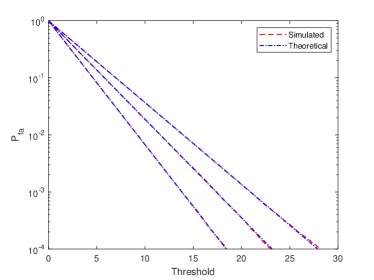
Figure 1: Probability of false alarm versus threshold in an experiment with $m=p=4$, $n=1000$, and $\rho=[0,0.02,0.05]$.

In this analysis, two distinct scenarios are considered. In first one, the noise covariance matrix is exactly known by the receiver, whereas in the second, a perturbed version, given by

$$\boldsymbol{\Sigma}_{\mathbf{N}}^{\prime}=\boldsymbol{\Sigma}_{{\mathbf{N}}}+\rho\mathbf{H}_{1}\mathbf{H}_{1}^{H},$$ (63)

is the one known by the receiver. In (63), $\mathbf{H}_{1}$ is generated as $\mathbf{H}$ and $\rho$ denotes a scaling factor quantifying the level of covariance matrix error.

Fig. 1 depicts the probability of false alarm for varying threshold in an experiment with $m=p=4$ antennas, $n=1000$, and mismatch levels $\rho=\{0,0.02,0.05\}$ (curve ordered from left to right). In the case of no mismatch, $\rho=0$, it compares the probability of false alarm obtained through Monte Carlo simulations with the theoretical result obtained in (33). As can be seen in the figure (leftmost curve), the agreement between theory and simulations is almost perfect. This agreement is also very good in the case of mismatch noise covariance matrices ($\rho\neq 0$), which demonstrates the accuracy of (39).

The next experiment analyzes the accuracy of the method used to compute the average probability of false alarm. In particular, we obtain the average probability for false alarm using Monte Carlo simulations and the proposed approximation in (50) with $N=1000$ in an experiment with $m=p=4$ antennas, $n=1000$. The errors in the noise correlation matrix are modeled as originating from a normal distribution $\mathcal{N}(\mathbf{0}_{m^{2}-m},\tau\mathbf{I}_{m^{2}})$, setting the mismatch levels at $\tau=\{0.1,0.2\}$. Fig. 2 illustrates these findings and includes a comparison to scenarios devoid of mismatch, thereby eliminating the need for averaging, for comparative analysis. The figure clearly demonstrates a strong concordance between the theoretical calculations and the simulation outcomes. This alignment between simulated results and theoretical predictions further corroborates the validity of (50).

Moreover, an advantage of employing (50) lies in its computational efficiency relative to (42). This efficiency stems from the rapid evaluation of the orthant probability for each sample. In contrast, (42) necessitates calculating orthant probabilities for every sample of the noise correlation matrix mismatch, a process that can be markedly time-intensive. Consequently, we have excluded it from the simulation.

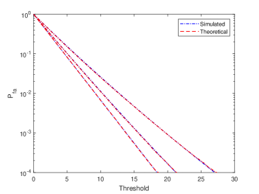
Figure 2: Average probability of false alarm versus threshold in an experiment with $m=p=4$, $n=1000$, and $\rho=[0,0.02,0.05]$.

VI-B Non-null Distribution

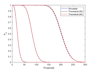
(a) Matched case

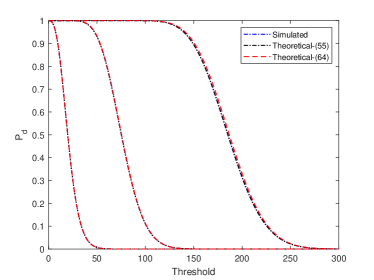
(b) Mismatched case

Figure 3: Probability of detection versus threshold in an experiment with $m=p=4$, $n=1000$, and $\text{SNR}=\{-20,-10,-7\}$ dBs.

TABLE I: Errors of Different Approximation Methods at Different SNRs

	Matched		Mismatched
SNR	​​​​$-20$ dB          $-10$ dB           $-7$ dB		​​​​$-20$ dB          $-10$ dB           $-7$ dB
​​Eq. (54)	$7.21\times 10^{-8}$    $1.35\times 10^{-7}$    $1.53\times 10^{-7}$	Eq. (55)	$1.17\times 10^{-7}$    $3.04\times 10^{-7}$    $1.03\times 10^{-6}$
​​Eq. (58)	$4.17\times 10^{-8}$    $2.38\times 10^{-6}$    $7.43\times 10^{-5}$	Eq. (59)	$1.18\times 10^{-7}$    $4.25\times 10^{-6}$    $7.87\times 10^{-5}$

We now turn our attention to the accuracy of the derived non-null distributions. For the matched scenario depicted, we compare the probability of detection obtained through Monte Carlo simulations with that predicted by (54) and (58). It should be noted that, in practical applications, the detection probability usually ranges in the vicinity of several tenths. Consequently, the figures utilize a linear scale for the detection probability, in contrast to the logarithmic scale used for the false alarm rate. Fig. 3(a) shows these values for an experiment with $m=p=4$, $n=1000$, and $\text{SNR}=\{-20,-10,-7\}$ dBs (from left to right), which shows the accuracy of the theoretical results. Fig. 3(b) considers a mismatched scenario, with $\rho=0.02$, for the same experiment and compares the simulations results with (55) and (59). Again, this analysis reveals a high degree of agreement between our theoretical findings and the corresponding simulations.

Additionally, Table I measures the approximation errors for (54) and (55), as well as for the low-SNR approximations, given by (58) and (59). Although the low-SNR approximations achieve worse accuracy, they are notably more straightforward to compute, as discussed in Section V-B, offering a practical advantage.

VI-C Detection Performance

In this section, we evaluate the detection performance of the proposed detector and compare it with a baseline white noise one-bit detector, as derived in [7]. We consider two key scenarios for this evaluation. In the first scenario, the noise covariance matrix is perfectly known to the receiver, and in the second, there is a mismatch in the noise covariance matrix due to estimation errors. For the mismatched scenario, we consider the model described in (63), with $\rho=\{0.01,0.02,0.03\}$. These values are intentionally selected to simulate moderate and significant noise mismatches, mirroring conditions frequently encountered in real-world applications. Our simulations involve a total of $n=2000$ samples with the SNR fixed at $-25$ dBs.

As illustrated in Fig. 4, which shows the ROC curves, the proposed detector shows enhanced detection performance in comparison to the white noise detector across all the considered levels of $\rho$. This finding highlights the critical role of considering the colored nature of the noise in detection processes. When $\rho=0.03$, a modest decline in detection performance is observed relative to scenarios with known noise covariance matrix. However, this decline is quantitatively less pronounced than typically expected for such degree of noise mismatch. This effect is attributed to the concurrent rightward shifts in both the null and non-null distributions caused by noise mismatches, as discussed in previous sections, which mitigates the extent of performance degradation. These results imply that at lower mismatch levels ($\rho=0.01,0.02$), the impact on detection performance is relatively negligible.

Furthermore, according to previous studies on one-bit covariance matrix estimation [30], estimation errors are often even lower than $\rho=0.02$, thereby supporting the reliability of the proposed detection method in practical scenarios where noise covariance matrix estimation is necessary. Nonetheless, the statistical analysis of noise mismatch impact is still crucial to maintain the CFAR property.

We also explore a more realistic scenario where the noise covariance matrix is estimated using noise-only samples. For this purpose, the observation interval is divided into two windows. The first window collects $n_{1}$ noise-only samples, which are used for the estimation of the noise covariance matrix using the algorithm presented in [30]. The signal transmission, of length $n_{2}$, then occurs in the subsequent phase. Since, contrary the proposed detector, the white noise detector does not use the noise covariance matrix, we exclude the training phase for this detector, dedicating the entire interval to signal transmission. To maintain a fair comparison, the total transmitted power of the signal is kept constant.

In the experiments with the proposed detector, we evaluate three configurations for the training sequence: $[n_{1},n_{2}]=[500,1500]$, $[1000,1000]$, and $[1500,500]$. These configurations are chosen to assess the impact of varying lengths of the training sequence on the detection performance. As shown in Fig. 5, the proposed detector consistently outperforms the white noise detector. Furthermore, the performance curve for all $[n_{1},n_{2}]$ settings closely mirrors that of the scenario with perfectly known noise covariance. This observation confirms that the current estimation approach yields sufficiently precise covariance matrix information, thereby ensuring the robust performance of our detection method. Hence, the effectiveness of the proposed detector in real-world scenarios, where noise covariance estimation is crucial, is underscored by this result.

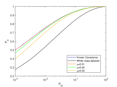
Figure 4: Detection performance under mismatched noise covariance.

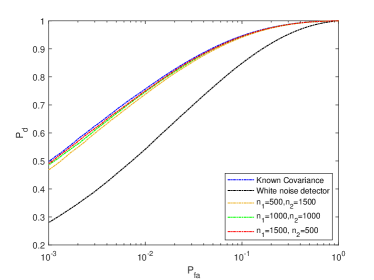
Figure 5: Impact of training sequence length on detection performance.

VII Conclusion

In this study, we derived a novel Rao’s test for one-bit target detection in MIMO radar systems operating for colored noise environments, generalizing our prior work [7]. The detector is designed as a weighted matched filter, with weights derived from orthant probabilities tied to noise covariance matrix elements. This approach shows enhanced robustness and significant performance gains in colored noise scenarios compared to the white noise detector [7]. Through comprehensive theoretical analysis, we obtained closed-form approximations for both the null and non-null distributions, enabling accurate calculations of false alarm and detection probabilities. We also assessed the impact of noise covariance matrix mismatch, highlighting how it increases the false alarm probability and providing the necessary adjustments to maintain the CFAR property. The analysis of the non-null distribution revealed that performance degradation due to covariance mismatch can be quantified by a decrease in the non-centrality parameter of a chi-squared distribution. Simulation results confirmed the effectiveness and practical applicability of the proposed detector in realistic radar detection scenarios.

VIII Acknowledgements

We would like to acknowledge the assistance of OpenAI’s GPT-4 in proofreading and enhancing the clarity of this manuscript. However, the final manuscript was reviewed and revised by the authors, who assume full responsibility for its form and content.

Appendix A Proof of Lemma 1

We consider $\mu_{1}$ as an example, as any other derivative can be obtained by a simple permutation of the components of the vector. First, we define the PDF of a zero-mean Gaussian

$$f(x_{1},\cdots,x_{k})=\phi_{k}(\mathbf{x};\mathbf{0}_{k},{\boldsymbol{\Sigma}}),$$ (64)

and rewrite (8) as

$$P(\boldsymbol{\mu},\boldsymbol{\Sigma})=\int_{-\infty}^{\mu_{1}}\int_{-\infty}^{\mu_{2}}\cdots\int_{-\infty}^{\mu_{k}}f(x_{1},\cdots,x_{k})dx_{1}\cdots dx_{k}.$$ (65)

Taking into account the definition of the the partial derivative of $P$ with respect to $\mu_{1}$, given by

$$\frac{\partial P}{\partial\mu_{1}}=\lim_{\Delta\mu_{1}\rightarrow 0}\frac{P(\boldsymbol{\mu}+\Delta\mu_{1}\mathbf{e}_{1},\boldsymbol{\Sigma})-P(\boldsymbol{\mu},\boldsymbol{\Sigma})}{\Delta\mu_{1}},$$ (66)

where $\mathbf{e}_{1}=[1,0,\cdots,0]^{T}$, we get

$$\frac{\partial P}{\partial\mu_{1}} =\lim_{\Delta\mu_{1}\rightarrow 0}\frac{\int_{\mu_{1}}^{\mu_{1}+\Delta\mu_{1}}\int_{-\infty}^{\mu_{2}}\cdots\int_{-\infty}^{\mu_{k}}f(x_{1},\cdots,x_{k})dx_{1}\cdots dx_{k}}{\Delta\mu_{1}}$$

$$=\int_{-\infty}^{\mu_{2}}\cdots\int_{-\infty}^{\mu_{k}}f(\mu_{1},x_{2},\cdots,x_{k})dx_{2}\cdots dx_{k}.$$ (67)

Now, using Bayes’s theorem to decompose the joint PDF, the derivative becomes

$$\frac{\partial P}{\partial\mu_{1}} =f_{x_{1}}(\mu_{1})\!\int_{-\infty}^{\mu_{2}}\!\!\!\!\!\cdots\!\!\int_{-\infty}^{\mu_{k}}\!\!f(x_{2},\cdots,x_{k}|x_{1}=\mu_{1})dx_{2}\cdots dx_{k}$$

$$=f_{x_{1}}(\mu_{1})P(\boldsymbol{\omega}(\boldsymbol{\mu},1),\mathbf{R}(\boldsymbol{\Sigma},1)),$$ (68)

where $\boldsymbol{\omega}(\boldsymbol{\mu},j)$ and $\mathbf{R}(\boldsymbol{\Sigma},j)$ are defined in the lemma. The proof follows from

$$f_{x_{1}}(\mu_{1})=\frac{1}{\sqrt{2\pi\boldsymbol{\Sigma}(1,1)}}.$$ (69)

Appendix B Proof of (25)

Firstly, we arrange all possibilities for $\mathbf{y}$ in ascending order of their binary forms, namely,

$$\boldsymbol{\tau}_{1} =[-1,\cdots,-1,-1]^{T}$$ (70a)

$$\boldsymbol{\tau}_{2} =[-1,\cdots,-1,+1]^{T}$$ (70b)

$$~{}~{}\!\vdots$$

$$\boldsymbol{\tau}_{\kappa} =[+1,\cdots,+1,+1]^{T}$$ (70c)

where $\kappa=2^{2m}$. We then define ${\boldsymbol{\Gamma}}_{j}={\rm diag}(\boldsymbol{\tau}_{j})$, and let

$$O_{j}=\Pr\{\underline{\mathbf{y}}=\boldsymbol{\tau}_{j};\boldsymbol{\theta}=\boldsymbol{\theta}_{0}\}=P(\mathbf{0},{\boldsymbol{\Gamma}}_{j}\mathbf{C}{\boldsymbol{\Gamma}}_{j}),$$ (71)

and

$$\mathbf{d}_{j}={\boldsymbol{\Gamma}}_{j}\left.\frac{\partial P(\boldsymbol{\mu},{\boldsymbol{\Gamma}}_{j}\mathbf{C}{\boldsymbol{\Gamma}}_{j})}{\partial\boldsymbol{\mu}}\right|_{\boldsymbol{\theta}=\boldsymbol{\theta}_{0}},$$ (72)

where the partial derivative of $P(\boldsymbol{\mu},{\boldsymbol{\Gamma}}_{j}\mathbf{C}{\boldsymbol{\Gamma}}_{j})$ is defined analogously to (24). Then, using (15) and (16), we obtain

$$\mathbb{E}\left[\left.\left(\frac{\partial\mathcal{L}(\underline{\mathbf{y}}_{i};\boldsymbol{\theta})}{\partial a}\right)^{2}\right|_{\boldsymbol{\theta}=\boldsymbol{\theta}_{0}}\right]\!=\!\sum_{j=1}^{\kappa}O_{j}\frac{(\mathbf{a}_{i}^{T}\mathbf{d}_{j})^{2}}{O_{j}^{2}}\!=\!\sum_{j=1}^{\kappa}\frac{(\mathbf{a}_{i}^{T}\mathbf{d}_{j})^{2}}{O_{j}},$$ (73)

and due to the independence of the observations

$$\mathbb{E}\left[\left.\left(\frac{\partial\mathcal{L}(\mathbf{Y};\boldsymbol{\theta})}{\partial a}\right)^{2}\right|_{\boldsymbol{\theta}=\boldsymbol{\theta}_{0}}\right]=\sum_{i=1}^{n}\sum_{j=1}^{\kappa}\frac{(\mathbf{a}_{i}^{T}\mathbf{d}_{j})^{2}}{O_{j}}.$$ (74)

Similarly, we have

$$\mathbb{E}\left[\left.\left(\frac{\partial\mathcal{L}(\mathbf{Y};\boldsymbol{\theta})}{\partial b}\right)^{2}\right|_{\boldsymbol{\theta}=\boldsymbol{\theta}_{0}}\right] =\sum_{i=1}^{n}\sum_{j=1}^{\kappa}\frac{(\mathbf{b}_{i}^{T}\mathbf{d}_{j})^{2}}{O_{j}},$$ (75)

$$\mathbb{E}\left[\left.\frac{\partial\mathcal{L}(\mathbf{Y};\boldsymbol{\theta})}{\partial a}\frac{\partial\mathcal{L}(\mathbf{Y};\boldsymbol{\theta})}{\partial b}\right|_{\boldsymbol{\theta}=\boldsymbol{\theta}_{0}}\right] =\sum_{i=1}^{n}\sum_{j=1}^{\kappa}\frac{\mathbf{a}_{i}^{T}\mathbf{d}_{j}\mathbf{b}_{i}^{T}\mathbf{d}_{j}}{O_{j}}.$$ (76)

Now, we study the “symmetric” properties of the orthant probabilities $\{O_{1},\cdots,O_{\kappa}\}$ and the derivative vectors $\{\mathbf{d}_{1},\cdots,\mathbf{d}_{\kappa}\}$. Since the noise is circular, the coherence matrix is invariant under the transformation

$$\mathbf{T}_{1}^{T}\mathbf{C}\mathbf{T}_{1}=\mathbf{C},$$ (77)

where

$$\mathbf{T}_{1}=\begin{bmatrix}\mathbf{0}_{m}&-\mathbf{I}_{m}\\ \mathbf{I}_{m}&\mathbf{0}_{m}\end{bmatrix}.$$ (78)

As a consequence, we have

$$O_{j}=\Pr\{\underline{\mathbf{y}}=\boldsymbol{\tau}_{j};\boldsymbol{\theta}=\boldsymbol{\theta}_{0}\}=\Pr\{\underline{\mathbf{y}}=\mathbf{T}_{1}\boldsymbol{\tau}_{j};\boldsymbol{\theta}=\boldsymbol{\theta}_{0}\}.$$ (79)

In addition, it is easily seen from $\eqref{derivatives_u_ab}$ that

$$\mathbf{b}_{i}=\mathbf{T}_{1}\mathbf{a}_{i}$$ (80)

Combining with (79) yields

$$\mathbf{d}_{j_{k}}=\mathbf{T}_{1}\mathbf{d}_{j},$$ (81)

where $j_{k}$ is the integer such that

$$\boldsymbol{\tau}_{j_{k}}=\mathbf{T}_{1}^{k}\boldsymbol{\tau}_{j},\quad k=1,2,\ldots$$ (82)

Using these symmetries, we can conclude that

$$\frac{(\mathbf{a}_{i}^{T}{\mathbf{d}}_{j})^{2}}{O_{j}}=\frac{(\mathbf{b}_{i}^{T}{\mathbf{d}}_{j_{k}})^{2}}{O_{j_{k}}},\quad k=1,2,\ldots$$ (83)

In addition, since

$$\boldsymbol{\tau}_{j}=\mathbf{T}_{1}^{4}\boldsymbol{\tau}_{j},$$ (84)

the set $\{1,\cdots,\kappa\}$ can be divided into $\kappa/4$ equal subsets with elements $j_{k},k=0,\cdots,3$, with the above definition of the index $j_{k}$. Consequently, the summations in (74) and (75) are given by the sum of $\kappa/4$ summations, given by

$$\sum_{k=0}^{3}\frac{(\mathbf{a}_{i}^{T}{\mathbf{d}}_{j_{k}})^{2}}{O_{j_{k}}}=\sum_{k=0}^{3}\frac{(\mathbf{b}_{i}^{T}{\mathbf{d}}_{j_{k}})^{2}}{O_{j_{k}}}.$$ (85)

Summing up these subsets yields

$$\sum_{j=1}^{\kappa}\frac{(\mathbf{a}_{i}^{T}{\mathbf{d}}_{j})^{2}}{O_{j}}=\sum_{j=1}^{\kappa}\frac{(\mathbf{b}_{i}^{T}{\mathbf{d}}_{j})^{2}}{O_{j}}.$$ (86)

Now we study the covariance term in (76). Similarly to our previous arguments, utilizing the symmetries, we can obtain the following relation

$$\frac{\mathbf{a}_{i}^{T}{\mathbf{d}}_{j}\mathbf{b}_{i}^{T}{\mathbf{d}}_{j}}{O_{j}}=-\frac{\mathbf{a}_{i}^{T}{\mathbf{d}}_{j_{k}}\mathbf{b}_{i}^{T}{\mathbf{d}}_{j_{k}}}{O_{j_{k}}},$$ (87)

which yields

$$\sum_{k=0}^{3}\frac{\mathbf{a}_{i}^{T}{\mathbf{d}}_{j_{k}}\mathbf{b}_{i}^{T}{\mathbf{d}}_{j_{k}}}{O_{j_{k}}}=0.$$ (88)

Hence, (76) becomes

$$\sum_{j=1}^{\kappa}\frac{\mathbf{a}_{i}^{T}{\mathbf{d}}_{j}\mathbf{b}_{i}^{T}{\mathbf{d}}_{j}}{O_{j}}=0.$$ (89)

and the FIM simplifies to

$$\mathbf{F}(\boldsymbol{\theta}_{0})=\upsilon^{2}\mathbf{I}_{2},$$ (90)

where

$$\upsilon^{2}=\sum_{i=1}^{n}\sum_{j=1}^{\kappa}\frac{(\mathbf{a}_{i}^{T}{\mathbf{d}}_{j})^{2}}{O_{j}}=\sum_{i=1}^{n}\sum_{j=1}^{\kappa}\frac{(\mathbf{b}_{i}^{T}{\mathbf{d}}_{j})^{2}}{O_{j}}.$$ (91)

Finally, defining

$${\mathbf{O}}={\rm diag}\left(O_{1},\cdots,O_{\kappa}\right),$$ (92)

and $\boldsymbol{\Delta}_{1}$, $\boldsymbol{\Delta}_{2}\in\mathbb{R}^{n\times\kappa}$ whose elements are

$${\boldsymbol{\Delta}}_{1}(i,j) =\mathbf{a}_{i}^{T}{\mathbf{d}}_{j}, {\boldsymbol{\Delta}}_{2}(i,j) =\mathbf{b}_{i}^{T}{\mathbf{d}}_{j},$$ (93)

$\upsilon^{2}$ can be rewritten as

$$\upsilon^{2} =\text{tr}\left(\boldsymbol{\Delta}_{1}^{T}\boldsymbol{\Delta}_{1}\mathbf{O}^{-1}\right)=\text{tr}\left(\boldsymbol{\Delta}_{2}^{T}\boldsymbol{\Delta}_{2}\mathbf{O}^{-1}\right).$$ (94)

This completes the proof of (25).

Appendix C Proof of Theorem 1

It is straightforward to obtain the asymptotic distribution of $\mathbf{w}$ and its mean, so this appendix computes the covariance matrix. Thus, we begin by defining

$$O^{\prime}_{j}=P(\mathbf{0},{\boldsymbol{\Gamma}}_{j}\mathbf{C}^{\prime}{\boldsymbol{\Gamma}}_{j}),$$ (95)

where $\mathbf{C}^{\prime}$ is the coherence matrix of $\boldsymbol{\Sigma}^{\prime}_{\underline{\mathbf{x}}}$. Following the same argument as (73) in Appendix B, we have

$$\mathbb{E}\left[\left(\frac{\partial\mathcal{L}(\underline{\mathbf{y}}_{i};\boldsymbol{\theta})}{\partial a}\right)^{2}\right]=\sum_{j=1}^{\kappa}O^{\prime}_{j}\frac{(\mathbf{a}_{i}^{T}\mathbf{d}_{j})^{2}}{O_{j}^{2}}=\sum_{j=1}^{\kappa}(\mathbf{a}_{i}^{T}\mathbf{d}_{j})^{2}\frac{O^{\prime}_{j}}{O^{2}_{j}}.$$ (96)

Likewise, we compute

$$\mathbb{E}\left[\left(\frac{\partial\mathcal{L}(\mathbf{Y};\boldsymbol{\theta})}{\partial a}\right)^{2}\right] =\sum_{i=1}^{n}\sum_{j=1}^{\kappa}O^{\prime}_{j}\frac{(\mathbf{a}_{i}^{T}\mathbf{d}_{j})^{2}}{O_{j}^{2}},$$ (97a)

$$\mathbb{E}\left[\left(\frac{\partial\mathcal{L}(\mathbf{Y};\boldsymbol{\theta})}{\partial b}\right)^{2}\right] =\sum_{i=1}^{n}\sum_{j=1}^{\kappa}O^{\prime}_{j}\frac{(\mathbf{b}_{i}^{T}\mathbf{d}_{j})^{2}}{O_{j}^{2}},$$ (97b)

$$\mathbb{E}\left[\frac{\partial\mathcal{L}(\mathbf{Y};\boldsymbol{\theta})}{\partial a}\frac{\partial\mathcal{L}(\mathbf{Y};\boldsymbol{\theta})}{\partial b}\right] =\sum_{i=1}^{n}\sum_{j=1}^{\kappa}O^{\prime}_{j}\frac{\mathbf{a}_{i}^{T}\mathbf{d}_{j}\mathbf{b}_{i}^{T}\mathbf{d}_{j}}{O_{j}^{2}}.$$ (97c)

Once again, by employing the circularity property, it can be shown that

$$O^{\prime}_{j}=O^{\prime}_{j_{k}},\quad k=1,2,3.$$ (98)

Combining with (87) and (97c), we have

$$\mathbb{E}\left[\frac{\partial\mathcal{L}(\mathbf{Y};\boldsymbol{\theta})}{\partial a}\frac{\partial\mathcal{L}(\mathbf{Y};\boldsymbol{\theta})}{\partial b}\right]=0.$$ (99)

Analogously, we obtain

$$\mathbb{E}\left[\left(\frac{\partial\mathcal{L}(\mathbf{Y};\boldsymbol{\theta})}{\partial a}\right)^{2}\right]=\mathbb{E}\left[\left(\frac{\partial\mathcal{L}(\mathbf{Y};\boldsymbol{\theta})}{\partial b}\right)^{2}\right]=\upsilon^{2}_{1},$$ (100)

where $\upsilon^{2}_{1}$, i.e., the variance in the mismatched case, is defined in (36). Consequently, the covariance matrix of $\mathbf{w}=[w_{1},w_{2}]^{T}$ is

$$\boldsymbol{\Sigma}_{w}=\upsilon^{2}_{1}\mathbf{I}_{2},$$ (101)

which completes the proof of Theorem 1.

Appendix D Proof of Theorem 2

The proof of Theorem 2 is based on Price’s Theorem [41], which is summarized in the following lemma. For clarity, we present its simplified version.

Lemma 2

Let $\mathbf{x}=[x_{1},\cdots,x_{k}]$ be a $k$-dimensional vector following a zero-mean Gaussian distribution with unit variances and coherence matrix $\mathbf{C}$. Consider $k$ nonlinear functions $g_{i}(x),i=1,2,\ldots,k$ and define the $k$th order correlation coefficient of the outputs as

$$R=\mathbb{E}\left[\prod_{i=1}^{k}g_{i}(x_{i})\right].$$ (102)

Then, the partial derivative of $R$ with respect to the elements of the coherence matrix $\mathbf{C}$ is given by

$$\frac{\partial R}{\partial\mathbf{C}(r,s)}=\mathbb{E}\left[g^{\prime}_{r}\left(x_{r}\right)g^{\prime}_{s}\left(x_{s}\right)\prod_{\begin{subarray}{c}i=1\\ i\neq r,s\end{subarray}}^{k}g_{i}(x_{i})\right],$$ (103)

where $g^{\prime}_{i}\left(x_{i}\right)$ is the derivative of $g_{i}\left(x_{i}\right)$ with respect to $x_{i}$ and $r<s$.

To proceed, we define

$$g_{i}(x)=\begin{cases}1,&x\geq 0,\\ 0,&x<0,\\ \end{cases}$$ (104)

for $i=1,\ldots,k,$ which yields

$$\mathbb{E}\left[\prod_{i=1}^{k}g_{i}(x_{i})\right]=\Pr\{x_{1}>0,\cdots,x_{k}>0\}=P(\mathbf{0}_{k},\mathbf{C}).$$ (105)

In addition, we have

$$g^{\prime}_{r}(x_{r})g^{\prime}_{s}(x_{s})=\delta(x_{r})\delta(x_{s}),$$ (106)

where $\delta(\cdot)$ is the Dirac delta function.

Therefore, Lemma 2 allows us to write the derivative of the orthant probability as

$$\frac{\partial P(\mathbf{0}_{k},\mathbf{C})}{\partial\mathbf{C}(r,s)}=\mathbb{E}\left[\delta(x_{r})\delta(x_{s})\right]\\ =\int_{-\infty}^{\infty}\cdots\int_{-\infty}^{\infty}\delta(x_{r})\delta(x_{s})\prod_{\begin{subarray}{c}i=1\\ i\neq r,s\end{subarray}}^{k}g_{i}(x_{i})f_{\mathbf{x}}(\mathbf{x})d\mathbf{x}.$$ (107)

Denoting $\bar{\mathbf{x}}$ as the remaining vector after removing $x_{r}$ and $x_{s}$ from $\mathbf{x}$, we can write $f_{\mathbf{x}}(\mathbf{x})=f_{\bar{\mathbf{x}}}(\bar{\mathbf{x}}|x_{r},x_{s})f_{x_{r},x_{s}}(x_{r},x_{s})$, which yields

$$\frac{\partial P(\mathbf{0}_{k},\mathbf{C})}{\partial\mathbf{C}(r,s)}=f_{x_{r},x_{s}}(0,0)\\ \times\int_{0}^{\infty}\cdots\int_{0}^{\infty}f_{\bar{\mathbf{x}}}(\bar{\mathbf{x}}|0,0)d\bar{\mathbf{x}}.$$ (108)

According to the conditional distribution of joint-Gaussian distribution [42], $\bar{\mathbf{x}}$ conditioned on $x_{r}=x_{s}=0$ is a zero mean Gaussian vector with covariance matrix

$$\tilde{\mathbf{C}}=[\boldsymbol{\Theta}(\boldsymbol{\Theta}(\mathbf{C}^{-1},r),s-1)]^{-1}.$$ (109)

Therefore, we obtain

$$\int_{0}^{\infty}\cdots\int_{0}^{\infty}f_{\bar{\mathbf{x}}}(\bar{\mathbf{x}}|0,0)d\bar{\mathbf{x}}=P(\mathbf{0}_{k-2},\tilde{\mathbf{C}}),$$ (110)

Finally, taking into account

$$f_{x_{r},x_{s}}(0,0)=\frac{1}{2\pi\sqrt{1-|\mathbf{C}(r,s)|^{2}}}$$ (111)

we obtain

$$\frac{\partial P(\mathbf{0}_{k},\mathbf{C})}{\partial\mathbf{C}(r,s)}=\frac{P(\mathbf{0}_{k-2},\tilde{\mathbf{C}})}{2\pi\sqrt{1-|\mathbf{C}(r,s)|^{2}}},$$ (112)

which completes the proof of Theorem 2.

Appendix E Proof of Theorem 3

The definition of the expectation allows us to write

$$\mathbb{E}\left[\frac{\partial\mathcal{L}(\underline{\mathbf{y}}_{i};\boldsymbol{\theta})}{\partial a}\right]=\sum_{j=1}^{\kappa}\mathbf{Q}(i,j)\frac{\mathbf{a}_{i}^{T}\mathbf{d}_{j}}{O_{j}},$$ (113)

and taking into account the independence of the observations, we get

$$\boldsymbol{\mu}_{w}(1) =\frac{1}{\upsilon}\mathbb{E}\left[\frac{\partial\mathcal{L}(\underline{\mathbf{Y}};\boldsymbol{\theta})}{\partial a}\right]=\frac{1}{\upsilon}\sum_{i=1}^{n}\sum_{j=1}^{\kappa}\mathbf{Q}(i,j)\frac{\mathbf{a}_{i}^{T}\mathbf{d}_{j}}{O_{j}}$$

$$=\frac{1}{\upsilon}\text{tr}(\mathbf{G}_{1}\mathbf{Q}^{T}).$$ (114)

Similarly, we have

$$\boldsymbol{\mu}_{w}(2)=\frac{1}{\upsilon}\mathbb{E}\left[\frac{\partial\mathcal{L}(\underline{\mathbf{Y}};\boldsymbol{\theta})}{\partial b}\right]=\frac{1}{\upsilon}\text{tr}(\mathbf{G}_{2}\mathbf{Q}^{T}).$$ (115)

Furthermore, the variance of $w_{1}$ is

$$\sigma_{1}^{2}=\mathbb{V}\left[\frac{\partial\mathcal{L}(\underline{\mathbf{Y}};\boldsymbol{\theta})\}}{\partial a}\right]=\sum_{i=1}^{n}\mathbb{V}\left[\frac{\partial\mathcal{L}(\underline{\mathbf{y}}_{i};\boldsymbol{\theta})}{\partial a}\right],$$ (116)

where each of the $n$ variances on the right-hand-side of the above expression can be obtained as

$$\mathbb{V}\left[\frac{\partial\mathcal{L}(\underline{\mathbf{y}}_{i};\boldsymbol{\theta})}{\partial a}\right]=\sum_{j=1}^{\kappa}\mathbf{Q}(i,j)\frac{(\mathbf{a}_{i}^{T}\mathbf{d}_{j})^{2}}{O_{j}^{2}}-\left(\sum_{j=1}^{\kappa}\mathbf{Q}(i,j)\frac{\mathbf{a}_{i}^{T}\mathbf{d}_{j}}{O_{j}}\right)^{2}.$$ (117)

Plugging (117) into (116) yields

$$\sigma_{1}^{2}=\sum_{i=1}^{n}\sum_{j=1}^{\kappa}\mathbf{Q}(i,j)\frac{(\mathbf{a}_{i}^{T}\mathbf{d}_{j})^{2}}{O_{j}^{2}}-\sum_{i=1}^{n}\left(\sum_{j=1}^{\kappa}\mathbf{Q}(i,j)\frac{\mathbf{a}_{i}^{T}\mathbf{d}_{j}}{O_{j}}\right)^{2}.$$ (118)

Similarly, we have

$$\sigma_{2}^{2}=\sum_{i=1}^{n}\sum_{j=1}^{\kappa}\mathbf{Q}(i,j)\frac{(\mathbf{b}_{i}^{T}\mathbf{d}_{j})^{2}}{O_{j}^{2}}-\sum_{i=1}^{n}\left(\sum_{j=1}^{\kappa}\mathbf{Q}(i,j)\frac{\mathbf{b}_{i}^{T}\mathbf{d}_{j}}{O_{j}}\right)^{2},$$ (119)

and

$$\sigma_{12}=\sum_{i=1}^{n}\sum_{j=1}^{\kappa}\mathbf{Q}(i,j)\frac{\mathbf{a}_{i}^{T}\mathbf{d}_{j}\mathbf{b}_{i}^{T}\mathbf{d}_{j}}{O_{j}^{2}}\\ -\sum_{i=1}^{n}\left(\sum_{j=1}^{\kappa}\mathbf{Q}(i,j)\frac{\mathbf{a}_{i}^{T}\mathbf{d}_{j}}{O_{j}}\right)\times\left(\sum_{j=1}^{\kappa}\mathbf{Q}(i,j)\frac{\mathbf{b}_{i}^{T}\mathbf{d}_{j}}{O_{j}}\right).$$ (120)

Appendix F Proof of (56) and (57)

Let us start with the matched noise covariance case. Given that $\beta$ is assumed to be of order $\mathcal{O}(n^{-\frac{1}{2}})$, it can be expressed as $\beta=\frac{1}{\sqrt{n}}(a_{0}+\imath b_{0})$. Recalling that

$$\mathbf{Q}(i,j) =P({\boldsymbol{\Gamma}}_{j}\mathbf{s}_{i},{\boldsymbol{\Gamma}}_{j}\mathbf{C}{\boldsymbol{\Gamma}}_{j}),$$ (121)

$$O_{j} =P(\mathbf{0}_{2m},{\boldsymbol{\Gamma}}_{j}\mathbf{C}{\boldsymbol{\Gamma}}_{j}),$$ (122)

when the SNR is sufficiently low, a first-order Taylor’s expansion of $\mathbf{Q}(i,j)$ at $[a,b]^{T}=[0,0]^{T}$ yields

$$\mathbf{Q}(i,j)=O_{j}+\frac{1}{\sqrt{n}}\left[a_{0}\left.\frac{\partial\mathbf{Q}(i,j)}{\partial a}\right|_{a=0}+b_{0}\left.\frac{\partial\mathbf{Q}(i,j)}{\partial b}\right|_{b=0}\right]\\ +\mathcal{O}(n^{-1}).$$ (123)

Taking into account (19), the derivatives are:

$$\left.\frac{\partial\mathbf{Q}(i,j)}{\partial a}\right|_{a=0} ={\mathbf{a}_{i}^{T}\mathbf{d}_{j}}={\boldsymbol{\Delta}_{1}(i,j)},$$ (124a)

$$\left.\frac{\partial\mathbf{Q}(i,j)}{\partial b}\right|_{b=0} ={\mathbf{b}_{i}^{T}\mathbf{d}_{j}}={\boldsymbol{\Delta}_{2}(i,j)},$$ (124b)

which yields

$$\mathbf{Q}=\mathbf{1}_{n}\mathbf{o}^{T}+\frac{1}{\sqrt{n}}\left(a_{0}\boldsymbol{\Delta}_{1}+b_{0}\boldsymbol{\Delta}_{2}\right)+\mathcal{O}(n^{-1}).$$ (125)

where $\mathbf{o}=[O_{1},\cdots,O_{\kappa}]^{T}$. Since $\mathbf{G}_{1}=\boldsymbol{\Delta}_{1}\mathbf{O}^{-1}$ and $\mathbf{G}_{2}=\boldsymbol{\Delta}_{2}\mathbf{O}^{-1}$, it can be shown that

$$\upsilon u_{1} =\text{tr}(\mathbf{G}_{1}\mathbf{Q}^{T})$$

$$=\mathbf{1}_{n}^{T}\boldsymbol{\Delta}_{1}\mathbf{1}_{\kappa}+\frac{1}{\sqrt{n}}\left[a_{0}\text{tr}\left(\boldsymbol{\Delta}_{1}^{T}\boldsymbol{\Delta}_{1}\mathbf{O}^{-1}\right)\right.$$

$$\left.\phantom{=}+b_{0}\text{tr}\left(\boldsymbol{\Delta}_{2}^{T}\boldsymbol{\Delta}_{1}\mathbf{O}^{-1}\right)\right]+\mathcal{O}(n^{-1}).$$ (126)

Using (81), we can easily conclude that $\mathbf{1}_{n}^{T}\boldsymbol{\Delta}_{1}\mathbf{1}_{\kappa}=0$. Moreover, as shown in Appendix B, $\text{tr}(\boldsymbol{\Delta}_{1}^{T}\boldsymbol{\Delta}_{2}\mathbf{O}^{-1})=0$ and $\text{tr}(\boldsymbol{\Delta}_{1}^{T}\boldsymbol{\Delta}_{1}\mathbf{O}^{-1})=\text{tr}(\boldsymbol{\Delta}_{2}^{T}\boldsymbol{\Delta}_{2}\mathbf{O}^{-1})=\upsilon^{2}$. Thus, we have:

$$u_{1}=\frac{\upsilon a_{0}}{\sqrt{n}}+\mathcal{O}(n^{-1})$$ (127)

and similarly,

$$u_{2}=\frac{\upsilon b_{0}}{\sqrt{n}}+\mathcal{O}(n^{-1}).$$ (128)

For the covariance matrix, using (118), the expression for $\sigma^{2}_{1}$ is

$$\sigma^{2}_{1}= \frac{1}{\upsilon^{2}}\mathbb{E}\left[\left(\frac{\partial\mathcal{L}\{{\mathbf{Y}}\}}{\partial a}\right)^{2}\right]-u_{1}^{2}$$

$$= 1+\frac{1}{\sqrt{n}\upsilon^{2}}\sum_{i=1}^{n}\sum_{j=1}^{\kappa}\frac{a_{0}(\mathbf{a}_{i}^{T}\mathbf{d}_{j})^{3}}{O_{j}^{2}}+\mathcal{O}(n^{-1})$$ (129)

A similar expression is derived for $\sigma^{2}_{2}$:

$$\sigma^{2}_{2}=1+\frac{1}{\sqrt{n}\upsilon^{2}}\sum_{i=1}^{n}\sum_{j=1}^{\kappa}\frac{b_{0}(\mathbf{a}_{i}^{T}\mathbf{d}_{j})^{3}}{O_{j}^{2}}+\mathcal{O}(n^{-1})$$ (130)

For the covariance $\sigma_{12}$, the expression is:

$${\sigma_{12}}= \frac{1}{\sqrt{n}\upsilon^{2}}\sum_{i=1}^{n}\sum_{j=1}^{\kappa}\frac{\mathbf{a}_{i}^{T}\mathbf{d}_{j}\mathbf{b}_{i}^{T}\mathbf{d}_{j}}{O_{j}^{2}}(a_{0}\mathbf{a}_{i}^{T}\mathbf{d}_{j}+b_{0}\mathbf{b}_{i}^{T}\mathbf{d}_{j})$$

$$+\mathcal{O}(n^{-1})$$ (131)

Given that $\upsilon^{2}$ is of order $n$, it follows that:

$$\boldsymbol{\Sigma}_{\mathbf{w}}=\mathbf{I}_{2}+\mathcal{O}(n^{-\frac{1}{2}}).$$ (132)

For the mismatched case where the true noise covariance matrix is $\boldsymbol{\Sigma}^{\prime}_{\underline{x}}$, we define:

$$\mathbf{a}^{\prime}_{i} ={\rm diag}(\boldsymbol{\Sigma}^{\prime}_{\underline{x}})^{-\frac{1}{2}}\left[\begin{array}[]{c}\mathbf{u}_{i}\\ \mathbf{v}_{i}\end{array}\right]$$ (133c)

$$\mathbf{b}^{\prime}_{i} ={\rm diag}(\boldsymbol{\Sigma}^{\prime}_{\underline{x}})^{-\frac{1}{2}}\left[\begin{array}[]{cc}-\mathbf{v}_{i}\\ \mathbf{u}_{i}\end{array}\right]$$ (133f)

$$\mathbf{d}^{\prime}_{j}(i) =\frac{1}{\sqrt{2\pi}}P(\mathbf{0},\mathbf{R}({\boldsymbol{\Gamma}}_{j}\mathbf{C}^{\prime}{\boldsymbol{\Gamma}}_{j},i)).$$ (133g)

Mirroring the arguments in the previous subsection, the partial derivatives are obtained as:

$$\frac{\partial\mathbf{Q}^{\prime}(i,j)}{\partial a}|_{a=0} =\mathbf{a}^{\prime T}_{i}\mathbf{d}^{\prime}_{j}={\boldsymbol{\Delta}^{\prime}_{1}(i,j)}$$ (134a)

$$\frac{\partial\mathbf{Q}^{\prime}(i,j)}{\partial b}|_{b=0} =\mathbf{b}^{\prime T}_{i}\mathbf{d}^{\prime}_{j}={\boldsymbol{\Delta}^{\prime}_{2}(i,j)}.$$ (134b)

Thus, the expressions for $u_{1}$ and $u_{2}$ are:

$$u_{1}= \frac{a_{0}}{\sqrt{n}\upsilon}\text{tr}(\boldsymbol{\Delta}_{1}^{T}\boldsymbol{\Delta}^{\prime}_{1}\mathbf{O}^{-1})$$ (135a)

$$u_{2}= \frac{b_{0}}{\sqrt{n}\upsilon}\text{tr}(\boldsymbol{\Delta}_{2}^{T}\boldsymbol{\Delta}^{\prime}_{2}\mathbf{O}^{-1}).$$ (135b)

Recalling that as proved in Appendix C, the covariance matrix for the mismatched case under $\mathcal{H}_{0}$ is $\frac{\upsilon_{1}^{2}}{\upsilon^{2}}\mathbf{I}_{2}$, following similar arguments, it can be concluded that when SNR is low:

$$\boldsymbol{\Sigma}_{\mathbf{w}}=\frac{\upsilon_{1}^{2}}{\upsilon^{2}}\mathbf{I}_{2}+\mathcal{O}(n^{-\frac{1}{2}}).$$ (136)

This completes the proof.

References

- [1] J. Ren and J. Li, “One-bit digital radar,” in Proc. 51st Asilomar Conf. Signals Syst. Comput., 2017, pp. 1142–1146.
- [2] B. Jin, J. Zhu, Q. Wu, Y. Zhang, and Z. Xu, “One-bit LFMCW radar: Spectrum analysis and target detection,” IEEE Trans. Aerosp. Electron. Syst., vol. 56, no. 4, pp. 2732–2750, Aug. 2020.
- [3] A. Ameri, A. Bose, J. Li, and M. Soltanalian, “One-bit radar processing with time-varying sampling thresholds,” IEEE Trans. Signal Process., vol. 67, no. 20, pp. 5297–5308, Oct. 2019.
- [4] F. Foroozmehr, M. Modarres-Hashemi, and M. M. Naghsh, “Transmit code and receive filter design for PMCW radars in the presence of one-bit ADC.” IEEE Trans. Aerosp. Electron. Syst., vol. 58, no. 4, pp. 3078–3089, Jan. 2022.
- [5] L. Ni, D. Zhang, Y. Sun, Y., N. Liu, J. Liang, and Q. Wan, “Detection and localization of one-bit signal in multiple distributed subarray systems.” IEEE Trans. Signal Process., vol. 71, pp. 2776–2791, Aug. 2023.
- [6] A. Ameri and M. Soltanalian, “One-bit radar processing for moving target detection,” Proc. IEEE Radar Conf. (RadarConf), 2019, pp. 1–6.
- [7] Y.-H. Xiao, D. Ramírez, P. J. Schreier, C. Qian, and L. Huang, “One-bit target detection in collocated MIMO radar and performance degradation analysis,” IEEE Trans. Veh. Technol., vol. 71, no. 9, pp. 9363–9374, Sep. 2022.
- [8] O. Bar-Shalom and A. J. Weiss, “DOA estimation using one-bit quantized measurements,” IEEE Trans. Aerosp. Electron. Syst., vol. 38, no. 3, pp. 868–884, Jul. 2002.
- [9] L. Feng, L. Huang, Q. Li, Z.-Q. He, and M. Chen, “An off-grid iterative reweighted approach to one-bit direction of arrival estimation.” IEEE Trans. Veh. Technol., vol. 72, no. 6, pp. 8134-8139, Jan. 2023.
- [10] K. Yu, Y. D. Zhang, M. Bao, Y. Hu, and Z. Wang, “DOA estimation from one-bit compressed array data via joint sparse representation,” IEEE Signal Process. Lett., vol. 23, no. 8, pp. 1279-1283, Sep. 2016.
- [11] C. L Liu and P. P. Vaidyanathan, “One-bit sparse array DOA estimation,” in Proc. IEEE Int. Conf. Acoust., Speech, Signal Process., New Orleans, LA, USA, Mar. 2017, pp. 3126–-3130
- [12] X. Shang, H. Zhu and J. Li, “Range-Doppler imaging via one-bit PMCW radar,” in 2020 IEEE 11th Sensor Array and Multichannel Signal Processing Workshop (SAM), Hangzhou, China, 2020, pp. 1–5.
- [13] X. Shang, J. Li, and P. Stoica, “Weighted SPICE algorithms for range-Doppler imaging using one-bit automotive radar,” IEEE J. Sel. Topics Signal Process., vol. 15, no. 4, pp. 1041–1054, Jun. 2021.
- [14] F. Xi, Y. Xiang, Z. Zhang, S. Chen, and A. Nehorai, “Joint angle and Doppler frequency estimation for MIMO radar with one-bit sampling: A maximum likelihood-based method,” IEEE Trans. Aerosp. Electron. Syst., vol. 56, no. 6, pp. 4734–4748, Dec. 2020.
- [15] F. Xi, Y. Xiang, S. Chen, and A. Nehorai, “Gridless parameter estimation for one-bit MIMO radar with time-varying thresholds,” IEEE Trans. Signal Process., vol. 68, pp. 1048–1063, Jan. 2020.
- [16] S. Yang, W. Yi, A. Jakobsson, Y. Wang, and H. Xiao, “Weak signal detection with low-bit quantization in colocated MIMO radar,” IEEE Trans. Signal Process., vol. 71, pp. 447–460, Feb. 2023.
- [17] S. Yang, Y. Lai, A. Jakobsson and W. Yi, “Hybrid quantized signal detection with a bandwidth-constrained distributed radar system,” IEEE Trans. Aerosp. Electron. Syst., vol. 59, no. 6, pp. 7835-7850, Jul., 2023.
- [18] M. Stein, A. Kurzl, A. Mezghani, and J. A. Nossek, “Asymptotic parameter tracking performance with measurement data of 1-bit resolution,” IEEE Trans. Signal Process., vol. 63, no. 22, pp. 6086-6095, Nov. 2015.
- [19] B. Zhao, L. Huang and W. Bao, “One-bit SAR imaging based on single-frequency thresholds,” IEEE Trans. Geosci. Remote Sens., vol. 57, no. 9, pp. 7017-7032, Sep. 2019.
- [20] S. Ge, D. Feng, S. Song, J. Wang and X. Huang, “Sparse logistic regression-based one-bit SAR imaging,” IEEE Trans. Geosci. Remote Sens., vol. 61, pp. 1-15, Oct. 2023.
- [21] A. Aubry, A. De Maio, L. Lan and M. Rosamilia, “Adaptive radar detection and bearing estimation in the presence of unknown mutual coupling,” IEEE Trans. Signal Process., vol. 71, pp. 1248-1262, Mar., 2023.
- [22] T. Wang, D. Xu, C. Hao, P. Addabbo and D. Orlando, “Clutter edges detection algorithms for structured clutter covariance matrices,” IEEE Trans. Process. Lett., vol. 29, pp. 642-646, Feb. 2022.
- [23] S. Han, L. Yan, Y. Zhang, P. Addabbo, C. Hao and D. Orlando, “Adaptive radar detection and classification algorithms for multiple coherent signals,” IEEE Trans. Signal Process., vol. 69, pp. 560-572, Dec. 2021.
- [24] W. Liu, Y. Wang, J. Liu, W. Xie, H. Chen, and W. Gu, “Adaptive detection without training data in colocated MIMO radar,” IEEE Trans. Aerosp. Electron. Syst., vol. 51, no. 3, pp. 2469-2479, Jul. 2015.
- [25] J. Liu, S. Zhou, W. Liu, J. Zheng, H. Liu, and J. Li, “Tunable adaptive detection in colocated MIMO radar,” IEEE Trans. Signal Process., vol. 66, no. 4, pp. 1080-1092, Feb. 2018.
- [26] O. Besson, “Rao, Wald, and Gradient tests for adaptive detection of Swerling I targets,” IEEE Trans. Signal Process., vol. 71, pp. 3043-3052, Aug. 2023.
- [27] A. De Maio, S. M. Kay and A. Farina, “On the invariance, coincidence, and statistical equivalence of the GLRT, Rao test, and Wald test,” IEEE Trans. Signal Process., vol. 58, no. 4, pp. 1967-1979, April 2010.
- [28] A. P. Shikhaliev and B. Himed, “GLR, Rao, and Wald tests for distributed parametric detection in subspace interference,” IEEE Trans. Signal Process., vol. 71, pp. 388-400, Jan. 2023.
- [29] S. M. Kay, Fundamentals of Statistical Signal Processing: Detection Theory. NJ, USA: Prentice Hall, 1998.
- [30] Y.-H. Xiao, L. Huang, D. Ramírez, C. Qian and H. C. So, “Covariance matrix recovery from one-bit data with non-zero quantization thresholds: algorithm and performance analysis,” IEEE Trans. Signal Process., vol. 71, pp. 4060-4076, Nov. 2023.
- [31] A. Eamaz, F. Yeganegi and M. Soltanalian, “Covariance recovery for one-bit sampled non-stationary signals with time-varying sampling thresholds,” IEEE Trans. Signal Process., vol. 70, pp. 5222-5236, 2022.
- [32] C.-L. Liu and Z.-M. Lin, “One-bit autocorrelation estimation with nonzero thresholds,” in Proc. IEEE Int. Conf. Acoust. Speech Signal Process., Toronto, Canada, Jun., 2021, pp. 4520-4524.
- [33] S. Dirksen, J. Maly, and H. Rauhut, “Covariance estimation under one-bit quantization,” Ann. Statist., vol. 50, no. 6, pp. 3538-3562, Dec. 2022.
- [34] P.-W. Wu, L. Huang, D. Ramírez, Y.-H. Xiao, and H. C. So, “One-bit spectrum sensing for cognitive radio,” IEEE Trans. Signal Process., vol. 72, pp. 549–564, 2024.
- [35] T. Koyama and A. Takemura, “Calculation of orthant probabilities by the holonomic gradient method,” Jpn. J. Ind. Appl. Math., vol. 32, no. 1, pp. 187–204, 2015.
- [36] T. Miwa, A. Hayter and S. Kuriki, “The evaluation of general non-centred orthant probabilities.” J. R. Statistical Society B, vol. 65, no.1, pp. 223-234, 2003.
- [37] D. Ramírez, I. Santamaría, and L. Scharf, Coherence: In Signal Processing and Machine Learning. Springer Nature, 2023.
- [38] J. P. Imhof, “Computing the distribution of quadratic forms in normal variables,” Biometrika, vol. 48, nos. 3–4, pp. 419–426, 1961.
- [39] G. Cui, H. Li, and M. Rangaswamy, “MIMO radar waveform design with constant modulus and similarity constraints,” IEEE Trans. Signal Process., vol. 62, no. 2, pp. 343–353, Jan. 2014.
- [40] O. Aldayel, V. Monga, and M. Rangaswamy, “Successive QCQP refinement for MIMO radar waveform design under practical constraints,” IEEE Trans. Signal Process., vol. 64, no. 14, pp. 3760–3774, Jul. 2016.
- [41] R. Price, “A useful theorem for nonlinear devices having Gaussian inputs,” IRE Trans. Inf. Theory, vol. 4, no. 2, pp. 69-72, Jun. 1958.
- [42] M. L. Eaton, Multivariate Statistics: A Vector Space Approach. NY, USA: Wiley, 1983.