Distribution-Aware Data Expansion with Diffusion Models

Abstract

The scale and quality of a dataset significantly impact the performance of deep models. However, acquiring large-scale annotated datasets is both a costly and time-consuming endeavor. To address this challenge, dataset expansion technologies aim to automatically augment datasets, unlocking the full potential of deep models. Current data expansion methods encompass image transformation-based and synthesis-based methods. The transformation-based methods introduce only local variations, resulting in poor diversity. While image synthesis-based methods can create entirely new content, significantly enhancing informativeness. However, existing synthesis methods carry the risk of distribution deviations, potentially degrading model performance with out-of-distribution samples. In this paper, we propose DistDiff, an effective data expansion framework based on the distribution-aware diffusion model. DistDiff constructs hierarchical prototypes to approximate the real data distribution, optimizing latent data points within diffusion models with hierarchical energy guidance. We demonstrate its ability to generate distribution-consistent samples, achieving substantial improvements in data expansion tasks. Specifically, without additional training, DistDiff achieves a 30.7% improvement in accuracy across six image datasets compared to the model trained on original datasets and a 9.8% improvement compared to the state-of-the-art diffusion-based method. Our code is available at https://github.com/haoweiz23/DistDiff

https://github.com/haoweiz23/DistDiff

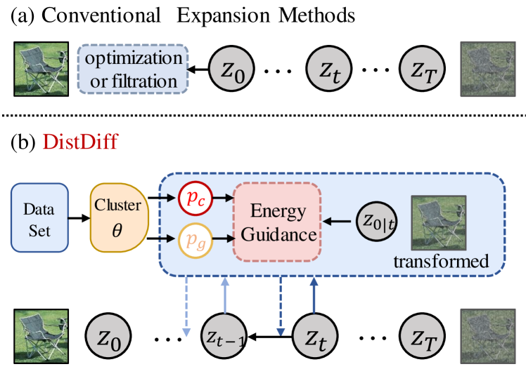
Figure 1: A comparison unveils distinctions between conventional data expansion methods and our innovative distribution-aware diffusion framework, benefiting from hierarchical clustering and multi-step energy guidance.

1 Introduction

A substantial number of training samples are essential for unlocking the full potential of deep networks. However, the manual collection and labeling of large-scale datasets are both costly and time-intensive. This makes it difficult to expand data-scarce datasets. Therefore, it is of great value to study how to expand high-quality training data in an efficient and scalable way.

Automatic data expansion technology can alleviate the data scarcity problem by augmenting or creating diverse samples, it mitigates the bottleneck associated with limited data, thereby improving model’s downstream performance and fostering greater generalization (Dunlap et al., 2023; Zhang et al., 2022). One simple yet effective strategy is employing image transformation techniques such as cropping, rotation, and erasing to augment samples (Shorten & Khoshgoftaar, 2019). Although these methods prove effective and have been widely applied in various fields, their pre-defined perturbations only introduce local variations to the images, thereby falling short in providing a diverse range of content change. In recent times, generative models have gained considerable attention (Goodfellow et al., 2020; Rombach et al., 2022; Ramesh et al., 2022; Saharia et al., 2022b; Nichol et al., 2021), exhibit impressive performance in various areas like image inpainting (Saharia et al., 2022a; Lugmayr et al., 2022), super-resolution (Ho et al., 2022b; Saharia et al., 2023), and video generation (Mei & Patel, 2023; Ho et al., 2022a). Generative models leverage text and image conditions to create images with entirely novel content, harnessing the expansive potential of data expansion. Nevertheless, there is a risk of generating images that deviate from the real data distribution. Therefore, when employing diffusion models for dataset expansion tasks, further research is necessary to ensure a match between synthetic data distributions and real data distributions.

There are several strategies aimed at mitigating the risk of distribution shift, which can be broadly categorized into two groups: training-based and training-free methods. The training-based methods (Moon et al., 2022; Xie et al., 2023; Ruiz et al., 2023) fine-tune pre-trained diffusion models to adapt target dataset, necessitating additional training costs and increasing the likelihood of overfitting on small-scale datasets. Other training-free methods (He et al., 2022; Feng et al., 2023) eliminate potentially noisy samples by designing optimizing and filtering strategies, but they still struggle to generate data that conforms to the real data distribution.

In this work, we propose a training-free data expansion framework, dubbed Distribution-Aware Diffusion (DistDiff) to optimize generation results. As shown in Figure 1, DistDiff initially approximates the true data distribution using class-level and group-level prototypes obtained through hierarchical clustering. Subsequently, DistDiff utilizes these prototypes to formulate two synergistic energy functions. A residual multiplicative transformation is then applied to the latent data points, enabling the generation of data distinct from the original. Following this, the hierarchical energy guidance process refines intermediate predicted data points, optimizing the diffusion model to generate data samples that are consistent with the underlying distribution. DistDiff ensures fidelity and diversity in the generated samples through distribution-aware energy guidance. Experimental results demonstrate that DistDiff outperforms advanced data expansion techniques, producing better expansion effects and significantly improving downstream model performance. Our contributions can be summarized as follows:

• We introduce a novel diffusion-based data expansion algorithm, named DistDiff, which facilitates distribution-consistent data augmentation without requiring re-training.

• By leveraging hierarchical prototypes to approximate data distribution, we propose an effective distribution-aware energy guidance at both class and group levels in the diffusion sampling process.

• The experimental results illustrate that our DistDiff is capable of generating high-quality samples, surpassing existing image transformation and synthesis methods significantly.

2 Related Work

2.1 Image Transformation

Traditional data augmentation techniques typically involve expanding the dataset through distortive transformations, aiming to enhance the model’s ability to capture data invariance and mitigate overfitting (Shorten & Khoshgoftaar, 2019). For instance, scale invariance is cultivated through random cropping and scaling, while rotation invariance is developed through random rotation and flipping. Methods like Random Erasing (Zhong et al., 2020) enhance model robustness against target occlusion by strategically obscuring portions of the target area. MixUp (Zhang et al., 2017) and CutMix (Yun et al., 2019) generate virtual samples by randomly blending content from two images. RandAugment (Cubuk et al., 2020) further boosts augmentation effectiveness by sampling from a diverse range of augmentation strategies. However, these approaches induce only subtle changes on the original data through transformation, deletion, and blend, leading to a lack of diversity. Moreover, these transformations are predefined and uniformly applied across the entire dataset, which may not be optimal for varying data types or scenarios.

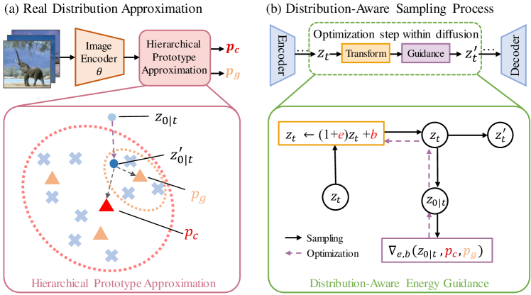
Figure 2: Overview of the DistDiff pipeline. DistDiff enhances the generation process in diffusion models with distribution-aware optimization. It approximates the real data distribution using hierarchical prototypes ${\bm{p}}_{c}$ and ${\bm{p}}_{g}$, optimizing the sampling process through distribution-aware energy guidance. Subsequently, original generated data point ${\bm{z}}_{t}$ is refined for improved alignment with the real distribution.

2.2 Image Synthesis

Generative data augmentation aims to leverage generative models to approximate the real data distribution, generating samples with novel content to enhance data diversity. GAN (Goodfellow et al., 2020) excels at learning data distributions and producing unseen samples in an unsupervised manner (Zhang et al., 2021; Gurumurthy et al., 2017; Antoniou et al., 2017). However, the necessity for separate GAN models for each category entails high training costs. Additionally, training processes of GAN are notoriously unstable, particularly with low-data regime, and suffer from mode collapse, resulting in a lack of diversity. In contrast, diffusion model-based methods (Yang et al., 2023) can offer better controllability and superior customization capabilities. Text-to-image models such as Stable Diffusion (Rombach et al., 2022), DALL-E 2 (Ramesh et al., 2022) and RPG (Yang et al., 2024b) have demonstrated the creation of compelling high-resolution images (Yang et al., 2024c; Zhang et al., 2024; Yang et al., 2024a). Recently, large-scale text-to-image models have been used for data augmentation. For example, He et al. (2022) utilized GLIDE (Nichol et al., 2021) to generate images, filtering low-confidence samples to enhance zero-shot and few-shot image classification performance. SGID (Li et al., 2023) leverages image descriptions generated by BLIP (Li et al., 2022) to enhance the semantic consistency of generated samples. Feng et al. (2023) filters out low-quality samples based on feature similarity between generated and reference images. GIF (Zhang et al., 2022) creates new informative samples through prediction entropy and feature divergence optimization. However, it’s crucial to note that datasets generated by existing methods may exhibit distribution shifts, impacting image classification performance significantly.

3 Preliminaries

In the context of a small-scale training dataset, the data expansion task is designed to augment the original dataset ${\mathcal{D}}_{o}=\{{\bm{x}}_{i},{\bm{y}}_{i}\}_{i=1}^{n_{o}}$ with a new set of synthetic samples, referred to as ${\mathcal{D}}_{s}=\{{\bm{x}}^{\prime}_{i},{\bm{y}}^{\prime}_{i}\}_{i=1}^{n_{s}}$. Here ${\bm{x}}_{i}$ and ${\bm{y}}_{i}$ represent the sample and its corresponding label, where $n_{o}$ and $n_{s}$ respectively denote the original sample quantity and the synthetic sample quantity. The objective is to enhance the performance of a deep learning model trained on both the original dataset ${\mathcal{D}}_{o}$ and the expanded dataset ${\mathcal{D}}_{s}$ compared to a model trained solely on the original ${\mathcal{D}}_{o}$. The crucial aspect lies in ensuring that the generated dataset is highly consistent with the distribution of the original dataset while being as informative as possible.

4 Method

In this study, we introduce a Distribution-Aware Data Expansion framework utilizing Stable Diffusion as a prior generation model. This framework guides the diffusion model based on hierarchical prototype guidance criteria. As illustrated in Figure 2, DistDiff initially employs a pretrained CLIP (Radford et al., 2021) image encoder to extract instance features and subsequently derives hierarchical prototypes to approximate the real data distribution. Next, for a given seed image and corresponding text prompts, we extract image’s latent feature and apply stochastic noise to it. Subsequently, in the denoising process, we optimize the latent features using a training-free hierarchical energy guidance process. Our optimization strategy ensures that the generated samples not only match the distribution but also carry new information to enhance model training.

4.1 Hierarchical Prototypes Approximate Data Distribution

Prototypes have been widely employed in class incremental learning methods to retain information about each class (Rebuffi et al., 2017; Masana et al., 2022). In this work, we propose two levels of prototypes to capture the original data distribution. Firstly, the class-level prototypes ${\bm{p}}_{\mathrm{c}}$ are obtained by averaging feature vectors within same class. The class vector aggregates high-level statistical information to characterize all samples from the same class as a collective entity. However, as class-level prototypes represent the class feature space as a single vector, potentially reducing informativeness, we further introduce group-level prototypes to capture the structure of the class feature space. Specifically, we divide all samples from the same class into $K$ groups using agglomerative hierarchical clustering, followed by averaging feature vectors within each group to obtain $K$ group prototypes ${\bm{p}}_{\mathrm{g}}=\{{\bm{p}}_{\mathrm{g}}^{1},{\bm{p}}_{\mathrm{g}}^{2},...,{\bm{p}}_{\mathrm{g}}^{K}\}$. Instances with similar patterns are grouped together. Transitioning from class-level to group-level, the prototypes encapsulate abstract distribution information of the class at different scales.

Thanks to these hierarchical prototypes, we design two function ${\mathcal{D}}_{\bm{\theta}}^{\mathrm{c}}$ and ${\mathcal{D}}_{\bm{\theta}}^{\mathrm{g}}$ to evaluate the degree of distribution matching:

$${\mathcal{D}}_{\bm{\theta}}^{\mathrm{c}}({\bm{x}},{\bm{p}}_{\mathrm{c}})=\lVert{\bm{\theta}}({\bm{x}})-{\bm{p}}_{\mathrm{c}}\rVert_{2}$$ (1)

$$\begin{gathered}{\mathcal{D}}_{\bm{\theta}}^{\mathrm{g}}({\bm{x}},{\bm{p}}_{\mathrm{g}})=\lVert{\bm{\theta}}({\bm{x}})-{\bm{p}}_{\mathrm{g}}^{j}\rVert_{2}\\ \mathrm{s.t.}j=\arg\max(\mathrm{cos}({\bm{\theta}}({\bm{x}}),\{{\bm{p}}_{\mathrm{g}}^{j}\}_{j=1}^{K}))\end{gathered}$$ (2)

where ${\bm{\theta}}(\cdot)$ means pre-trained feature extractor, which could be CLIP or other deep models.

Note that these two functions evaluate the score of distribution matching from two perspectives. The value will be lower when ${\bm{x}}$ is more consistent with the real distribution. As shown in Figure 2 (a), ${\mathcal{D}}_{\bm{\theta}}^{\mathrm{c}}$ gauges the distance of sample features to the class center, resulting in low scores for easy samples while high scores for hard samples that are situated at the boundaries of the distribution. On the other hand, ${\mathcal{D}}_{\bm{\theta}}^{\mathrm{g}}$ assesses distance from the group-level, offering lower scores for hard samples, while still maintaining relatively high scores for outlier samples. Consequently, these two scores mutually reinforce each other and are indispensable.

4.2 Transform Data Points

Given a reference sample $({\bm{x}},{\bm{y}})$, the pre-trained large-scale diffusion model ${\mathcal{G}}$ can generate new samples ${\bm{x}}^{\prime}$ with novel content. We formalize this process as ${\bm{x}}^{\prime}={\mathcal{G}}(\Phi({\bm{x}})+\delta)$, where $\Phi({\bm{x}})$ represents the latent feature representation and $\delta$ is the perturbation applied to latent features. Drawing inspiration from GIF (Zhang et al., 2022), we introduce residual multiplicative transformation to the latent feature ${\bm{z}}=\Phi({\bm{x}})$ using randomly initialized channel-level noise ${\bm{e}}\sim{\mathcal{U}}(0,1)$ and ${\bm{b}}\sim{\mathcal{N}}(0,1)$. We impose an $\epsilon$-ball constraint on the transformed feature to control the degree of adjustment within a reasonable range, i.e., $\lVert{\bm{z}}-\tilde{{\bm{z}}}\rVert_{\infty}\leq\epsilon$, and derive $\tilde{{\bm{z}}}$ as follows.

$$\tilde{{\bm{z}}}={\mathcal{P}}_{z,\epsilon}(\tau({\bm{z}}))={\mathcal{P}}_{z,\epsilon}((1+{\bm{e}}){\bm{z}}+{\bm{b}})$$ (3)

where $\tau(\cdot)$ represents the transformation function and ${\mathcal{P}}_{z,\epsilon}(\cdot)$ denotes the projection of the transformed feature $\tilde{{\bm{z}}}$ onto the $\epsilon$-ball of the original latent feature ${\bm{z}}$.

Now, the key challenge lies in optimizing ${\bm{e}}$ and ${\bm{b}}$ to create new samples that align closely with the real data distribution.

4.3 Distribution-Aware Diffusion Generation

In a typical diffusion sampling process, the model iteratively predicts noise to progressively map the noisy ${\bm{z}}_{T}$ into clean ${\bm{z}}_{0}$. While existing data expansion methods treat the generative model as a black box, focusing on filtering or optimizing the final generated ${\bm{z}}_{0}$. The importance of the intermediate sampling stage is ignored, which plays a crucial role in ensuring data quality, especially as the image begins to take on a stable shape appearance. Diverging from prior approaches, we advocate for intervention at the intermediate denoising step for optimization.

Specifically, we first introduce energy guidance into standard reverse sampling process to optimize the transformation using Equation 4. As our energy guidance step is applied to the transformed data point, the transformed data point $\tilde{{\bm{z}}_{t}}$ is denoted as ${\bm{z}}_{t}$ for simplicity.

$${\bm{e}}^{\prime}={\bm{e}}-\rho\nabla_{{\bm{e}}}\varepsilon({\bm{z}}_{t},c)$$ (4)

$${\bm{b}}^{\prime}={\bm{b}}-\rho\nabla_{{\bm{b}}}\varepsilon({\bm{z}}_{t},c)$$

here $\rho$ is the learning rate and $\varepsilon({\bm{z}}_{t},{\bm{c}})$ is the energy function measuring the compatibility between the transformed noisy data point ${\bm{z}}_{t}$ and the given condition ${\bm{c}}$, representing the real data distribution in this work. Equation 4 guides the sampling process and generates distribution-consistent samples. After that, the optimized ${\bm{z}}^{\prime}_{t}$ is obtained via Equation 3. However, directly measuring the distance between intermediate results ${\bm{z}}_{t}$ with condition ${\bm{c}}$ is impractical due to the difficulty in finding a pre-trained network that provides meaningful guidance when the input is noisy.

To address this issue, we leverage the capability that the diffusion model can predict the noise added to ${\bm{z}}_{t}$, and thus predict a clean data point ${\bm{z}}_{0|t}$, as shown in Equation 5. Then, the new energy function ${\mathcal{D}}_{\bm{\theta}}({\bm{z}}_{0|t},{\bm{c}})$ based on the predicted clean data point is constructed to approximate $\varepsilon({\bm{z}}_{t},{\bm{c}})$.

$${\bm{z}}_{0|t}=\frac{{\bm{z}}_{t}-\sqrt{1-\alpha_{t}}\psi({\bm{z}}_{t},t)}{\sqrt{\alpha_{t}}}$$ (5)

where $\alpha_{t}$ represents the noise scale and $\psi$ is the learned denoising network. Finally, we employ hierarchical prototypes ${\bm{p}}_{\mathrm{c}}$ and ${\bm{p}}_{\mathrm{g}}$ as conditions to construct our energy guidance in the following manner:

$${\bm{e}}^{\prime}={\bm{e}}-\rho\nabla_{e}({\mathcal{D}}_{\bm{\theta}}^{\mathrm{c}}({\bm{z}}_{0|t},{\bm{p}}_{\mathrm{c}})+\mathcal{D}_{\bm{\theta}}^{\mathrm{g}}({\bm{z}}_{0|t},{\bm{p}}_{\mathrm{g}}))$$ (6)

$${\bm{b}}^{\prime}={\bm{b}}-\rho\nabla_{b}({\mathcal{D}}_{\bm{\theta}}^{\mathrm{c}}({\bm{z}}_{0|t},{\bm{p}}_{\mathrm{c}})+\mathcal{D}_{\bm{\theta}}^{\mathrm{g}}({\bm{z}}_{0|t},{\bm{p}}_{\mathrm{g}}))$$

Unlike existing methods that exclusively optimize the final sampling result ${\bm{z}}_{0}$, our approach focuses on optimizing intermediate denoising steps within the sampling process. The detailed algorithm is shown in Algorithm 1. This novel strategy leads to substantial improvements in optimization results and will be further explored in Section 5.4.

Algorithm 1 Optimization Process of our proposed DistDiff

  Input: Hierarchical prototypes ${\bm{p}}_{\mathrm{c}}$ and ${\bm{p}}_{\mathrm{g}}$; Data point ${\bm{z}}_{T}$; Optimization step $M$; Pre-defined parameters $\beta_{t}$; Perturbation constraint $\epsilon$; Pre-trained feature extractor ${\bm{\theta}}$; Denoising network $\psi$.

  for $t=T-1,\dots,0$ do

     $\delta\sim{\mathcal{N}}(\mathbf{0},\mathbf{I})$ if $t>0$, else $\delta=0$.

     ${\bm{z}}_{t}=(1+\frac{1}{2}\beta_{t+1}){\bm{z}}_{t+1}+\beta_{t+1}\psi({\bm{z}}_{t+1},t+1)+\sqrt{\beta_{t+1}}\delta$

     if $t=M$ then

        Initialize ${\bm{e}}\sim{\mathcal{U}}(0,1)$, ${\bm{b}}\sim{\mathcal{N}}(0,1)$.

        ${\bm{z}}_{t}=(1+{\bm{e}}){\bm{z}}_{t}+{\bm{b}}$

        ${\bm{z}}_{0|t}=({\bm{z}}_{t}-\sqrt{1-\alpha_{t}}\psi({\bm{z}}_{t},t))/\sqrt{\alpha_{t}}$

        ${\mathcal{D}}_{\bm{\theta}}^{\mathrm{c}}({\bm{z}}_{0|t},{\bm{p}}_{\mathrm{c}})=\lVert{\bm{\theta}}({\bm{z}}_{0|t})-{\bm{p}}_{\mathrm{c}}\rVert_{2}$

        $\mathcal{D}_{\bm{\theta}}^{\mathrm{g}}({\bm{z}}_{0|t},{\bm{p}}_{\mathrm{g}})=\lVert{\bm{\theta}}({\bm{z}}_{0|t})-{\bm{p}}_{\mathrm{g}}\rVert_{2}$

        ${\bm{g}}_{t}={\mathcal{D}}_{\bm{\theta}}^{\mathrm{c}}({\bm{z}}_{0|t},{\bm{p}}_{\mathrm{c}})+\mathcal{D}_{\bm{\theta}}^{\mathrm{g}}({\bm{z}}_{0|t},{\bm{p}}_{\mathrm{g}})$

        update ${\bm{e}}^{\prime},{\bm{b}}^{\prime}\leftarrow{\arg\min}_{e,b}{\bm{g}}_{t}$ (Equation 6)

        update ${\bm{z}}_{t}\leftarrow{\bm{z}}^{\prime}_{t}={\mathcal{P}}_{z,\epsilon}((1+{\bm{e}}^{\prime}){\bm{z}}_{t}+{\bm{b}}^{\prime})$

     end if

  end for

  Output: ${\bm{z}}_{0}$.

5 Experiments

5.1 Experimental Setups

Datasets.

We assess the performance of DistDiff across six image classification datasets, encompassing diverse tasks such as general object classification (Caltech-101 (Fei-Fei et al., 2004), CIFAR100-Subset (Krizhevsky et al., 2009)), fine-grained classification (Pets (Parkhi et al., 2012), Cars (Krause et al., 2013), Flowers (Nilsback & Zisserman, 2008)), and textual classification (DTD (Cimpoi et al., 2014)). More details are provided in the appendix.

Compared Methods.

We conduct a comparative analysis between DistDiff and conventional image transformation methods, as well as diffusion-based expansion methods. Traditional image transformation techniques considered in the comparison comprise RandAugment (Cubuk et al., 2020), Cutout (DeVries & Taylor, 2017), and GridMask (Chen et al., 2020). For diffusion-based methods, we include the direct application of stable diffusion for data expansion, as well as the most recent state-of-the-art method, GIF-SD (Zhang et al., 2022).

5.2 Implementation details

In our experimental setup, we implement DistDiff based on CLIP VIT-B/32 and Stable Diffusion v1-4 (Rombach et al., 2022). The images created by SD have a resolution of $512\times 512$ for all datasets.

Throughout the diffusion process, we employ the DDIM (Song et al., 2020) sampler for a $50$-step latent diffusion, with hyper-parameters for strength set at $0.9$ and scale at $50$. The $\epsilon$ in Equation 3 is 0.8 by default. We assign $K=3$ to each class when constructing group-level prototypes, the learning rate $\rho$ is 0.1, and optimization step $M$ is set to $30$ unless specified otherwise.

After expansion, we train the classification model from scratch for $100$ epochs based on the expanded datasets. During model training, we process images through random resizing to $224\times 224$ using random rotation and random horizontal flips. Our optimization strategy involves using the SGD optimizer with a momentum of $0.9$, and cosine LR decay with an initial learning rate of $0.1$. All results are averaged over three runs with different random seeds.

Table 1: The main results of data expansion. All the experiments all trained from scratch based on ResNet-50, and all datasets are scaled up by $5\times$. The Compared Expansion methods results are cited from (Zhang et al., 2022).

Method	Caltech	Cars	Flowers	DTD	CIFAR100-S	Pets	Average
Original dataset	36.8	23.8	77.3	21.6	43.6	29.0	38.7
Compared Expansion methods
Cutout (DeVries & Taylor, 2017)	48.9	24.1	77.1	22.9	44.3	37.1	42.4 (+3.7)
GridMask (Chen et al., 2020)	49.1	26.2	78.1	24.1	46.7	37.1	43.6 (+4.9)
RandAugment (Cubuk et al., 2020)	51.0	33.9	81.1	26.1	46.9	37.7	46.1 (+7.4)
GIF-SD (Zhang et al., 2022)	54.4	60.6	81.8	33.9	61.1	65.7	59.6 (+20.9)
DistDiff (ours)	74.1	81.5	91.6	40.8	62.0	66.1	69.4 (+30.7)

Table 2: Model performance of various backbones trained across six datasets.

Caltech-101	ResNet-50	ResNeXt-50	WideResNet-50	MobileNet V2	Average
Original dataset	36.8 $\pm$ 2.1	45.7 $\pm$ 2.2	37.6 $\pm$ 1.2	63.4 $\pm$ 0.5	45.9
5x Expanded by GIF-SD	54.4 $\pm$ 0.7	52.8 $\pm$ 1.1	60.7 $\pm$ 0.3	55.6 $\pm$ 0.5	55.9 (${\color[rgb]{1,0,0}+10.0}$)
5x Expanded by DistDiff	74.1 $\pm$ 0.7	77.6 $\pm$ 0.8	73.4 $\pm$ 0.4	80.4 $\pm$ 0.8	76.4 (${\color[rgb]{1,0,0}+30.5}$)
Cars	ResNet-50	ResNeXt-50	WideResNet-50	MobileNet V2	Average
Original dataset	23.8 $\pm$ 1.3	60.6 $\pm$ 1.9	44.1 $\pm$ 1.1	57.5 $\pm$ 1.1	46.5
5x Expanded by GIF-SD	60.6 $\pm$ 1.9	64.1 $\pm$ 1.3	75.1 $\pm$ 0.4	60.2 $\pm$ 1.6	65.0 (${\color[rgb]{1,0,0}+18.5}$)
5x Expanded by DistDiff	81.5 $\pm$ 1.1	82.12 $\pm$ 0.3	80.2 $\pm$ 0.5	82.9 $\pm$ 0.6	81.7 (${\color[rgb]{1,0,0}+35.2}$)
Flowers	ResNet-50	ResNeXt-50	WideResNet-50	MobileNet V2	Average
Original dataset	77.3 $\pm$ 2.0	80.0 $\pm$ 1.7	79.8 $\pm$ 0.4	90.1 $\pm$ 0.5	81.8
5x Expanded by GIF-SD	82.1 $\pm$ 1.7	82.0 $\pm$ 1.2	85.0 $\pm$ 0.6	89.0 $\pm$ 0.1	84.5 (${\color[rgb]{1,0,0}+2.7}$)
5x Expanded by DistDiff	91.6 $\pm$ 1.2	93.9 $\pm$ 0.3	92.7 $\pm$ 0.4	93.6 $\pm$ 0.1	93.0 (${\color[rgb]{1,0,0}+11.2}$)
DTD	ResNet-50	ResNeXt-50	WideResNet-50	MobileNet V2	Average
Original dataset	21.6 $\pm$ 1.1	26.1 $\pm$ 0.7	22.0 $\pm$ 1.8	34.7 $\pm$ 2.3	26.1
5x Expanded by GIF-SD	33.9 $\pm$ 0.9	33.3 $\pm$ 1.6	40.6 $\pm$ 1.7	40.8 $\pm$ 1.1	37.2 (${\color[rgb]{1,0,0}+11.1}$)
5x Expanded by DistDiff	40.8 $\pm$ 0.2	45.9 $\pm$ 0.6	40.9 $\pm$ 1.2	50.8 $\pm$ 0.2	44.6 (${\color[rgb]{1,0,0}+18.5}$)
CIFAR100-S	ResNet-50	ResNeXt-50	WideResNet-50	MobileNet V2	Average
original dataset	43.6 $\pm$ 2.5	42.4 $\pm$ 1.9	45.4 $\pm$ 1.7	54.8 $\pm$ 0.3	46.6
5x Expanded by GIF-SD	61.1 $\pm$ 0.8	59.0 $\pm$ 0.7	64.4 $\pm$ 0.2	62.4 $\pm$ 0.1	61.7 (${\color[rgb]{1,0,0}+15.2}$)
5x Expanded by DistDiff	62.0 $\pm$ 0.4	60.9 $\pm$ 0.9	64.6$\pm$0.3	63.6 $\pm$ 0.1	62.8 (${\color[rgb]{1,0,0}+16.2}$)
Pets	ResNet-50	ResNeXt-50	WideResNet-50	MobileNet V2	Average
original dataset	29.0 $\pm$ 2.9	32.2 $\pm$ 3.8	30.0 $\pm$ 3.8	51.9 $\pm$ 3.3	35.8
5x Expanded by GIF-SD	65.8 $\pm$ 0.6	56.5 $\pm$ 0.6	70.9 $\pm$ 0.4	60.6 $\pm$ 0.5	63.5 (${\color[rgb]{1,0,0}+27.7}$)
5x Expanded by DistDiff	66.1 $\pm$ 0.1	67.9 $\pm$ 0.5	67.3 $\pm$ 0.9	73.2 $\pm$ 0.2	68.6 (${\color[rgb]{1,0,0}+32.9}$)

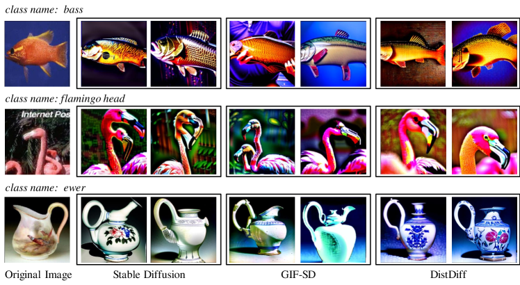
Figure 3: Visualization results. We present generated examples for Caltech-101 by stable diffusion (Rombach et al., 2022), GIF-SD (Zhang et al., 2022), and our DistDiff. More visualization results can be found in appendix.

5.3 Main Results

Quantitative Analysis.

As illustrated in Table 1, DistDiff demonstrates an average improvement of 30.9% across six image datasets compared to models trained on the original datasets. In comparison to model trained on the conventional augmentations, e.g., RandAugment, DistDiff achieves an average improvement of 23.3%. Furthermore, when compared with the state-of-the-art diffusion-based method GIF-SD, DistDiff exhibits an average improvement of 9.8%, affirming its superiority in dataset expansion. Notably, the improvement achieved by DistDiff on the fine-grained dataset (Pets) is significantly higher than that on the general dataset (CIFAR100-S). This observation suggests that DistDiff’s strategy of characterizing the original distribution through hierarchical prototypes holds a substantial advantage, particularly on fine-grained categories with significant intra-class variance.

Qualitative Analysis.

Figure 3 displays samples generated by image transformation methods, including SD, GIF-SD, and our DistDiff method. The results indicate that the SD model and GIF-SD model may generate samples that fall outside the distribution of the original dataset, leading to a shift in the distribution of the generated dataset and consequently diminishing the model’s classification performance. In contrast, DistDiff can not only generate entirely new samples but also maintain distribution consistency and sample diversity, thereby surpassing existing methods.

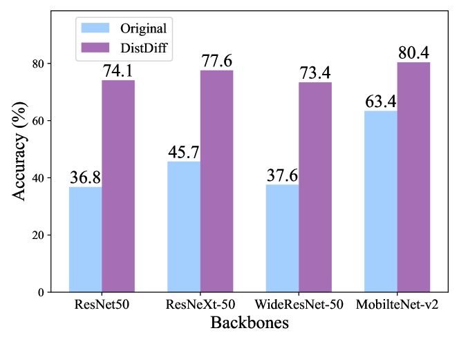
Figure 4: Performance of different backbones trained from scratch on $5\times$ expanded caltech-101 dataset by DistDiff.

Different Backbone Analysis.

We conduct an in-depth assessment of the expanded datasets generated by DistDiff across four distinct backbones: ResNet50 (He et al., 2016), ResNeXt-50 (Xie et al., 2017), WideResNet-50 (Zagoruyko & Komodakis, 2016), and MobileNetv2 (Sandler et al., 2018). These backbones are trained from scratch on $5\times$ expanded Caltech-101 dataset by DistDiff. The results presented in Figure 4 affirm that our innovative Distdiff methodology is effective and versatile across a spectrum of architectures. Additional experiments across various datasets are summarized in Table 2. It is evident that our DistDiff consistently delivers significant improvements across diverse architectures and datasets.

5.4 Ablation study

Hierarchical Prototypes.

We delved further into how each component of DistDiff impacts its data expansion performance. As depicted in Table 3, utilizing both ${\bm{p}}_{\mathrm{c}}$ and ${\bm{p}}_{\mathrm{g}}$ contributes to enhancing the model’s expansion performance, showcasing their ability to optimize the generated sample distribution at the class-level and group-level, respectively. Moreover, combining ${\bm{p}}_{\mathrm{c}}$ and ${\bm{p}}_{\mathrm{g}}$ results in a further performance improvement, validating the effectiveness of integrating representations from different hierarchical levels. Additionally, with the introduction of our approach, the Fréchet Inception Distance (FID) values notably decrease, indicating that our proposed FID effectively optimizes the model to generate samples more aligned with the real distribution, thereby reducing the domain gap between the generated dataset and the real dataset.

Table 3: Ablation of hierarchical prototypes in DistDiff for expanding Caltech-101 by $5\times$.

${\bm{p}}_{\mathrm{c}}$	${\bm{p}}_{\mathrm{g}}$	Accuracy $\uparrow$	FID $\downarrow$
		$67.9\pm 1.7$	196.2
	✓	$71.5\pm 0.3$	194.1
✓		$72.5\pm 0.8$	193.8
✓	✓	$74.1\pm 0.7$	192.3

Table 4: Ablation of optimization step $M$ in DistDiff for expanding Caltech-101 by $5\times$.

$M$	0	10	20	30	40
Accuracy	70.4	71.4	72.1	74.1	67.7

Table 5: Ablation of the number $K$ of group-level prototypes in DistDiff for expanding Caltech-101 by $5\times$.

$K$	1	2	3	4
Accuracy	72.5	73.1	74.1	73.4

Augmentation within Diffusion.

In the application of energy guidance, perturbation is introduced at the $M$-th step, and these subsequent predicted data points are optimized. Theoretically, optimizing predictions at different stages yields distinct effects. Our exploration focused on the optimization step $M$, and the experimental results are illustrated in Table 4. When $M$ is small, indicating optimization at a later stage (i.e., the refinement stage), the change in generated results is already minimal, resulting in relatively consistent optimization outcomes. Conversely, when $M$ increases, corresponding to optimization at an intermediate stage (i.e., the semantic stage), the generated results are in the stage of forming semantics and exhibit significant changes. Hence, this stage plays a crucial role in determining the final generated results. Furthermore, there is a decline in performance during the early chaos stage ($M$=40), as the data points in this initial phase are too chaotic to establish an optimal target for optimization. We observed that achieving higher data expansion performance is possible when optimized in the semantic stage, with optimal results obtained when $M$=30.

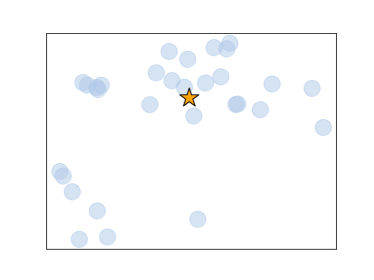
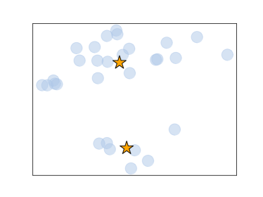
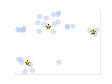
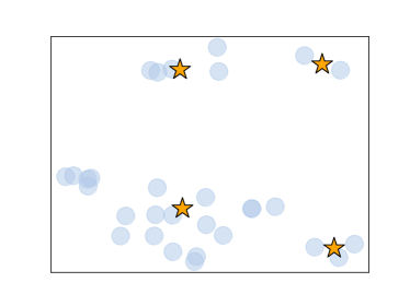
(a) $K=1$ (b) $K=2$ (c) $K=3$ (d) $K=4$

Figure 5: The visualization of group-level prototypes alongside original sample features. Here $\bullet$ is the sample point and $\star$ is group-level prototype. We can see that by selecting an appropriate number $K$, these prototypes effectively span the feature space, providing an approximation of the real data distribution.

Determination of Group-Level Prototype Number $K$.

The determination of the number $K$ of group-level prototypes is crucial for accurately approximating the real data distribution. In Table 5, we compare the outcomes associated with varying numbers of prototypes. The results highlight that the optimal number of prototypes is found at $K=3$. We posit that an insufficient number of prototypes may impede the characterization of the real distribution, leading to diminished performance. Conversely, an excessive number of prototypes may lead to overfitting of noisy sample points, also resulting in suboptimal performance. Furthermore, we present a visualization analysis of group-level prototypes in Figure 5. The visual representation demonstrates that an appropriate number of group-level prototypes can effectively cover the real distribution space, aligning with the underlying motivation of our DistDiff.

Table 6: Comparison of introducing multiple optimization steps in DistDiff for expanding Caltech-101 by $5\times$.

Strategy	Accuracy(%)
1 step ($30$)	74.1
Strategy 1
2 steps ($30,31$)	74.4
4 steps ($28,29,30,31$)	72.8
Strategy 2
3 steps ($30,15,0$)	72.5
4 steps ($30,20,10,0$)	72.2

More Optimization Steps.

Furthermore, a natural idea arises regarding the potential improvement in effectiveness through the optimization of more optimization steps. Therefore, we further explored two optimization strategies: optimizing more steps in semantic stage (Strategy 1) and optimizing both the semantic and refine stages (Strategy 2). In Strategy 1, we employ hierarchical energy guidance across several consecutive steps within the semantic stage. In Strategy 2, our hierarchical energy guidance is applied across distinct stages. As shown in Table 6, the results in the first row of Strategy1 indicate that increasing the optimization steps in semantic stages enhances performance. However, a subsequent increase in optimization steps leads to a performance decline. This can be attributed to an excessive optimization strength on energy guidance causing data distortion. In addition, Strategy2 did not yield positive results. When optimizing by combining the semantic and refining stages, the content of the refining stage has already taken shape. Introducing energy-guided optimization to this stage may diminish the advantage gained through optimization in the semantic stage, leading to suboptimal performance.

5.5 Further Analysis

Benefits for Pretrained Model.

Models pre-trained on large-scale datasets can yield superior performance than those trained from scratch. To assess the advantages of DistDiff in fine-tuning scenarios, we fine-tuned ImageNet1k (Deng et al., 2009) pre-trained ResNeXt-50 on diverse datasets. Table 7 demonstrates that DistDiff also achieves significant improvements in fine-tuning pre-trained models.

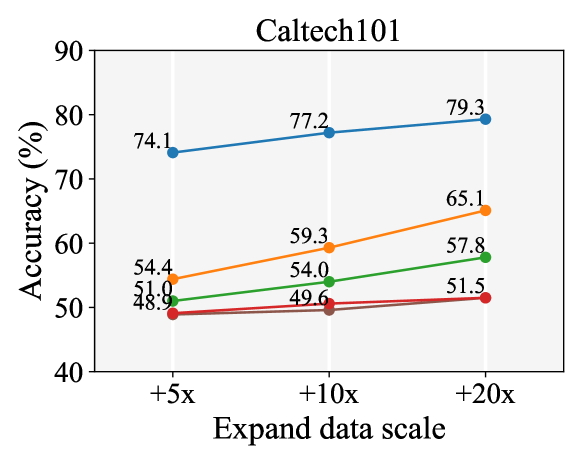
Figure 6: Comparison results of ResNet-50 trained from scratch across expanded datasets with different expansion scales.

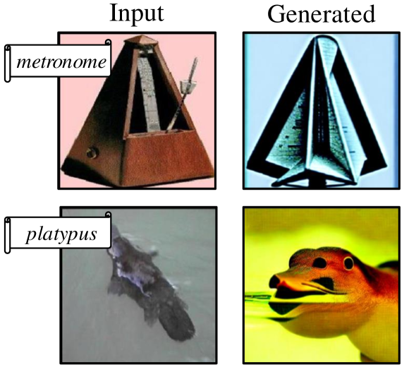
Figure 7: Failure cases visualization of our DistDiff.

Table 7: Experiments of fine-tuning pretrained model. Here we finetune ImageNet-1k pretrained ResNeXt-50 model on original and $5\times$ expanded Caltech-101 dataset generated by DistDiff.

Method	Original	DistDiff
Accuracy ($\%$)	80.5	87.8 (+7.8)

Benefits of Large Scale Expansion.

We conducted an extensive analysis of data expansion at a larger expansion scale, and the findings are presented in Figure 6. As the data augmentation scale increases, the corresponding improvement in accuracy also enlarges. It demonstrates that our DistDiff have superior efficiency in data expansion compared to existing methods. For instance, the accuracy achieved with our $5\times$ expansion surpasses even the 20x expanded dataset obtained by other methods.

Failure Case Analysis.

Figure 7 illustrates some failure cases generated by DistDiff framework. Given its training-free nature, the fidelity of a few generated samples remains constrained, particularly in scenarios involving domain shifts. Despite the presence of visual distortions in these cases, it is noteworthy that these samples are generated through our distribution-aware energy guidance. Consequently, they still exhibit the ability to approximate the real distribution space.

6 Conclusion

This paper presents DistDiff, a Distribution-Aware Data Expansion method employing a stable diffusion model for data expansion. The proposed method optimizes the diffusion process to align the synthesized data distribution with the real data distribution. Specifically, DistDiff constructs hierarchical prototypes to effectively represent the real data distribution and refines intermediate features within the sampling process using energy guidance. We evaluate our method through extensive experiments on six datasets, showcasing its superior performance over existing methods.

Impact Statements

This paper presents work whose goal is to advance the field of Machine Learning. There are many potential societal consequences of our work, none which we feel must be specifically highlighted here.

Appendix A More Details of Datasets.

Table 8 provides the detailed statistics of six experimental datasets, including Caltech-101 (Fei-Fei et al., 2004), CIFAR100-Subset (Krizhevsky et al., 2009), StandardCars (Krause et al., 2013), OxfordFlowers (Nilsback & Zisserman, 2008), OxfordPets (Parkhi et al., 2012) and DTD (Cimpoi et al., 2014). Cifar100-Subset is a subset that randomly sampled from original trainset with 100 samples per class. Specifically, our evaluation encompasses datasets that span diverse scenarios, incorporating generic objects, fine-grained categories, and textural images. These diverse datasets enable a comprehensive assessment of both the robustness and effectiveness of our proposed methods. Additionally, we also provide the text template employed in the conditional diffusion process in Table 9.

Table 8: Summary of our six experimental datasets.

Name	Number of Classes	Size (Train / Test)	Description
Caltech-101	102	3060 / 6085	Recognition of generic objects
CIFAR100-Subset	100	10000 / 10000	Recognition of generic objects
StandardCars	196	8144 / 8041	Fine-grained classification of cars
OxfordFlowers	102	6552 / 818	Fine-grained classification of flowers
OxfordPets	37	3680 / 3669	Fine-grained classification of pets
DTD	47	3760 / 1880	Texture classification

Table 9: Text templates for six experimental datasets.

Name	Template
Caltech-101	“a photo of a [class].”
CIFAR100-Subset	“a photo of a [class].”
StandardCars	“A photo of a [class] car.”
OxfordFlowers	“a photo of a [class], a type of flower.”
OxfordPets	“A photo of a pet [class].”
DTD	“[class] texture.”

Appendix B More Results Analyses

B.1 More Training Iterations

While data expansion methods enrich data diversity, they also lead to an increase in training iterations. A natural inquiry arises as to whether simply increasing the training iterations on the original dataset can yield performance improvements. To explore this, we extended the training time by $6\times$ (600 epochs) on the Caltech-101 original dataset. The experimental accuracy increased from 36.8% to 52.5%, but still significantly lagged behind DistDiff’s 74.1%. This observation confirms that the efficacy of our DistDiff method is not solely attributed to the increased training iterations.

B.2 More Ablations

In Table 3, we showcased the effectiveness of our hierarchical designs on Caltech-101 (Fei-Fei et al., 2004). In this section, we further conducted an ablation study on the textural datasets (DTD (Cimpoi et al., 2014)). The results, as presented in Table 10 affirm that both class-level and group-level prototypes contribute significantly to performance gains and are deemed indispensable.

Table 10: Ablation study of hierarchical prototypes on $5\times$ expanded DTD.

${\bm{p}}_{\mathrm{c}}$	${\bm{p}}_{\mathrm{g}}$	Accuracy $\uparrow$
		$35.2\pm 0.4$
	✓	$37.9\pm 0.6$
✓		$38.4\pm 0.3$
✓	✓	$40.8\pm 0.2$

B.3 Computational Efficiency

Our DistDiff is not only training-free but also highly efficient in processing. As illustrated in Figure 2 in the main text, DistDiff introduces only a few optimization steps in the original diffusion process. We analyze the time costs of our methods. Stable Diffusion generates per sample in 30 seconds on average, while our DistDiff achieves the same in 32 seconds, with the increased time costs being negligible. We can draw the conclusion that DistDiff achieves a notable improvement over stable diffusion without guidance, with only a slight increase in computation costs.

B.4 More Visualization Results

In this section, we provide more generated results comparison across six datasets in Figure 8–31 to demonstrate the effectiveness of DistDiff. These visualizations confirm that our approach can generate samples with more distribution-consistent patterns.

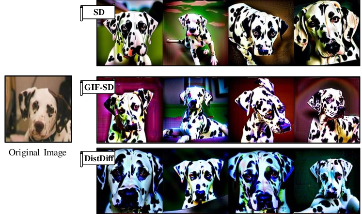
Figure 8: Visualization comparison of generated results on Caltech-101 (Example 1).

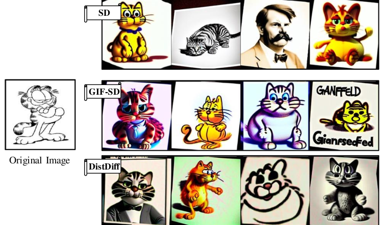
Figure 9: Visualization comparison of generated results on Caltech-101 (Example 2).

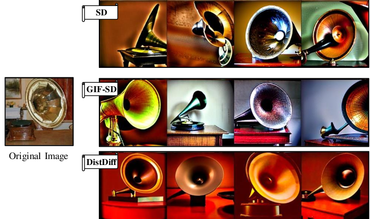
Figure 10: Visualization comparison of generated results on Caltech-101 (Example 3).

Figure 11: Visualization comparison of generated results on Caltech-101 (Example 4).

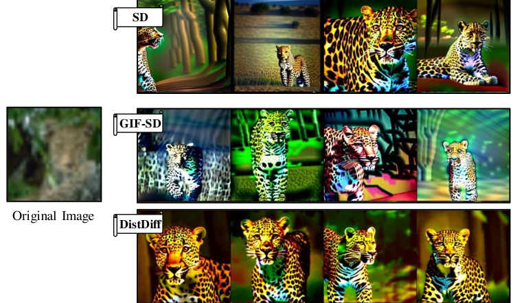
Figure 12: Visualization comparison of generated results on CIFAR100-S (Example 1).

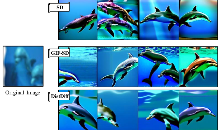
Figure 13: Visualization comparison of generated results on CIFAR100-S (Example 2).

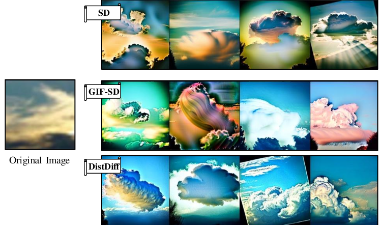
Figure 14: Visualization comparison of generated results on CIFAR100-S (Example 3).

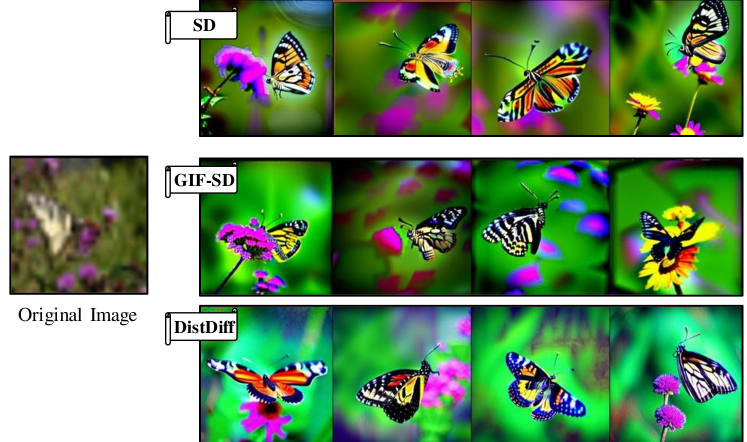
Figure 15: Visualization comparison of generated results on CIFAR100-S (Example 4).

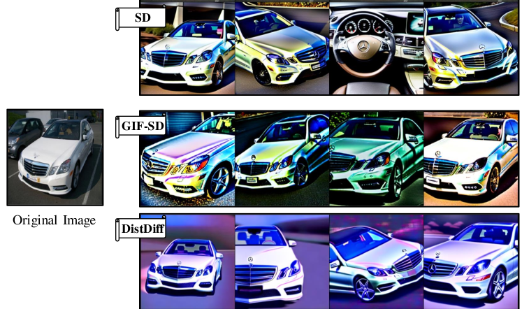
Figure 16: Visualization comparison of generated results on StanfordCars (Example 1).

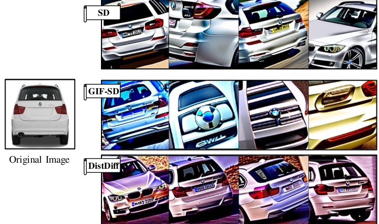
Figure 17: Visualization comparison of generated results on StanfordCars (Example 2).

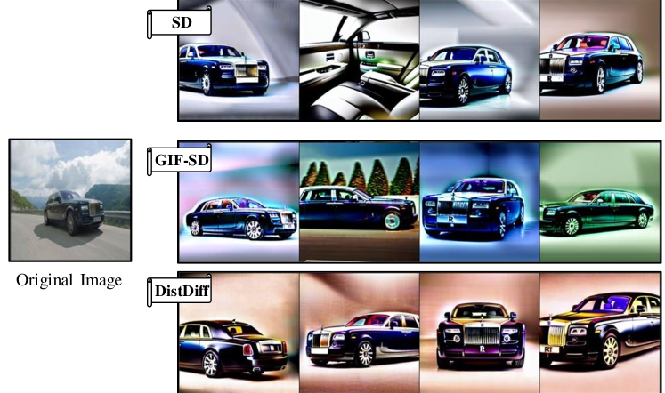
Figure 18: Visualization comparison of generated results on StanfordCars (Example 3).

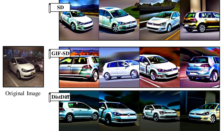
Figure 19: Visualization comparison of generated results on StanfordCars (Example 4).

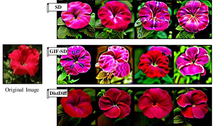
Figure 20: Visualization comparison of generated results on OxfordFlowers (Example 1).

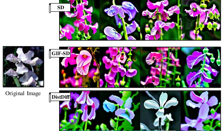
Figure 21: Visualization comparison of generated results on OxfordFlowers (Example 2).

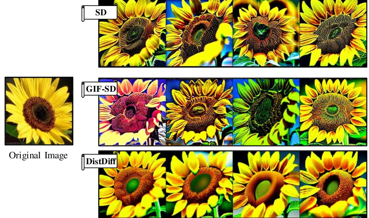
Figure 22: Visualization comparison of generated results on OxfordFlowers (Example 3).

Figure 23: Visualization comparison of generated results on OxfordFlowers (Example 4).

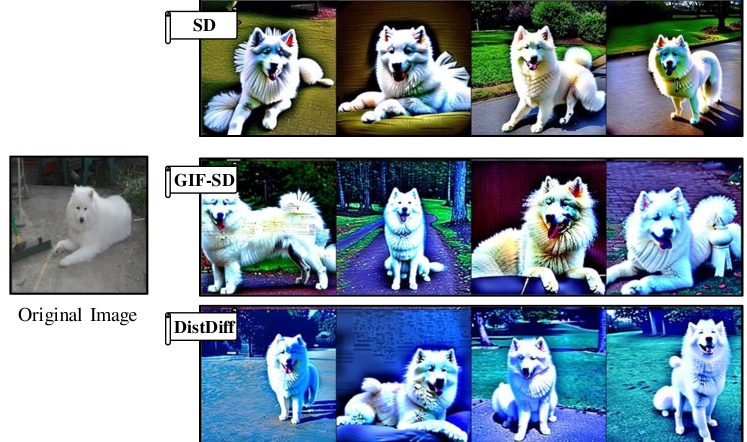
Figure 24: Visualization comparison of generated results on OxfordPets (Example 1).

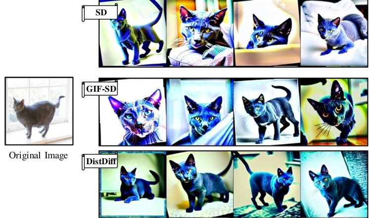
Figure 25: Visualization comparison of generated results on OxfordPets (Example 2).

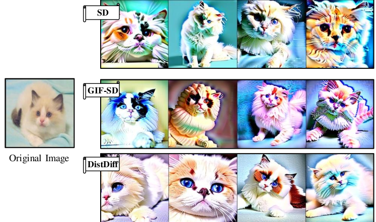
Figure 26: Visualization comparison of generated results on OxfordPets (Example 3).

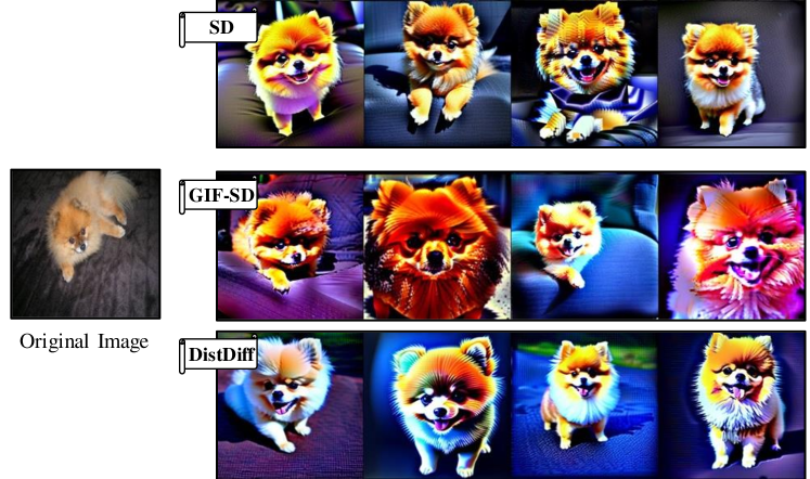
Figure 27: Visualization comparison of generated results on OxfordPets (Example 4).

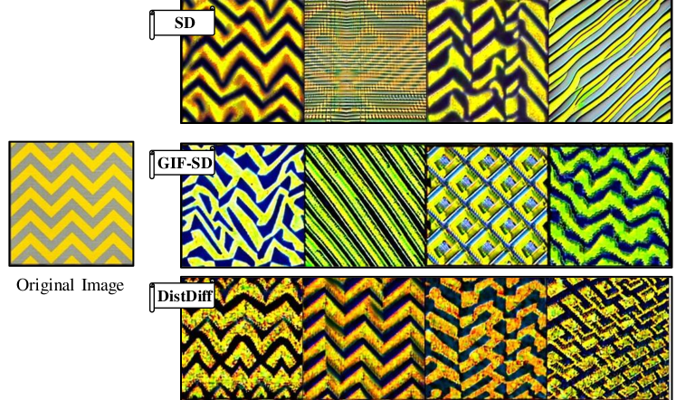
Figure 28: Visualization comparison of generated results on DTD (Example 1).

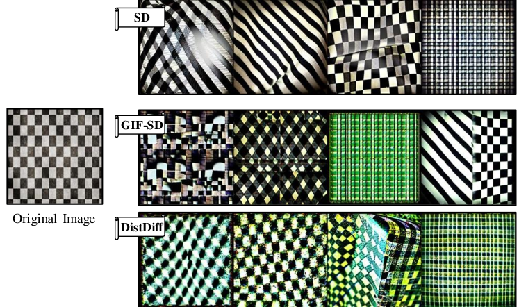
Figure 29: Visualization comparison of generated results on DTD (Example 2).

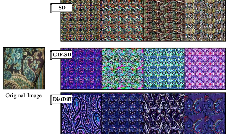
Figure 30: Visualization comparison of generated results on DTD (Example 3).

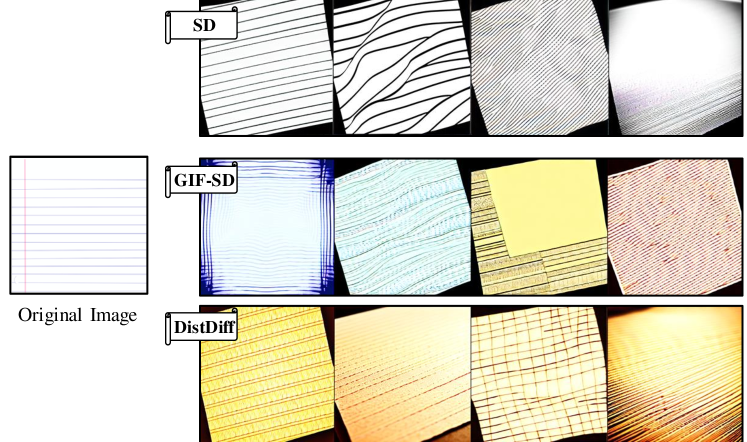
Figure 31: Visualization comparison of generated results on DTD (Example 4).

References

- Antoniou et al. (2017) Antoniou, A., Storkey, A., and Edwards, H. Data augmentation generative adversarial networks. arXiv preprint arXiv:1711.04340, 2017.
- Chen et al. (2020) Chen, P., Liu, S., Zhao, H., and Jia, J. Gridmask data augmentation. arXiv preprint arXiv:2001.04086, 2020.
- Cimpoi et al. (2014) Cimpoi, M., Maji, S., Kokkinos, I., Mohamed, S., and Vedaldi, A. Describing textures in the wild. In Proceedings of the IEEE conference on computer vision and pattern recognition, pp. 3606–3613, 2014.
- Cubuk et al. (2020) Cubuk, E. D., Zoph, B., Shlens, J., and Le, Q. V. Randaugment: Practical automated data augmentation with a reduced search space. In Proceedings of the IEEE/CVF conference on computer vision and pattern recognition workshops, pp. 702–703, 2020.
- Deng et al. (2009) Deng, J., Dong, W., Socher, R., Li, L.-J., Li, K., and Fei-Fei, L. Imagenet: A large-scale hierarchical image database. In 2009 IEEE conference on computer vision and pattern recognition, pp. 248–255. Ieee, 2009.
- DeVries & Taylor (2017) DeVries, T. and Taylor, G. W. Improved regularization of convolutional neural networks with cutout, 2017.
- Dunlap et al. (2023) Dunlap, L., Umino, A., Zhang, H., Yang, J., Gonzalez, J. E., and Darrell, T. Diversify your vision datasets with automatic diffusion-based augmentation. arXiv preprint arXiv:2305.16289, 2023.
- Fei-Fei et al. (2004) Fei-Fei, L., Fergus, R., and Perona, P. Learning generative visual models from few training examples: An incremental bayesian approach tested on 101 object categories. In 2004 conference on computer vision and pattern recognition workshop, pp. 178–178. IEEE, 2004.
- Feng et al. (2023) Feng, C.-M., Yu, K., Liu, Y., Khan, S., and Zuo, W. Diverse data augmentation with diffusions for effective test-time prompt tuning. In Proceedings of the IEEE/CVF International Conference on Computer Vision, pp. 2704–2714, 2023.
- Goodfellow et al. (2020) Goodfellow, I., Pouget-Abadie, J., Mirza, M., Xu, B., Warde-Farley, D., Ozair, S., Courville, A., and Bengio, Y. Generative adversarial networks. Communications of the ACM, 63(11):139–144, 2020.
- Gurumurthy et al. (2017) Gurumurthy, S., Kiran Sarvadevabhatla, R., and Venkatesh Babu, R. Deligan: Generative adversarial networks for diverse and limited data. In Proceedings of the IEEE conference on computer vision and pattern recognition, pp. 166–174, 2017.
- He et al. (2016) He, K., Zhang, X., Ren, S., and Sun, J. Deep residual learning for image recognition. In Proceedings of the IEEE conference on computer vision and pattern recognition, pp. 770–778, 2016.
- He et al. (2022) He, R., Sun, S., Yu, X., Xue, C., Zhang, W., Torr, P., Bai, S., and Qi, X. Is synthetic data from generative models ready for image recognition? arXiv preprint arXiv:2210.07574, 2022.
- Ho et al. (2022a) Ho, J., Chan, W., Saharia, C., Whang, J., Gao, R., Gritsenko, A., Kingma, D. P., Poole, B., Norouzi, M., Fleet, D. J., and Salimans, T. Imagen video: High definition video generation with diffusion models. 2022a.
- Ho et al. (2022b) Ho, J., Saharia, C., Chan, W., Fleet, D. J., Norouzi, M., and Salimans, T. Cascaded diffusion models for high fidelity image generation. J. Mach. Learn. Res., 23(1), jan 2022b.
- Krause et al. (2013) Krause, J., Deng, J., Stark, M., and Fei-Fei, L. Collecting a large-scale dataset of fine-grained cars. 2013.
- Krizhevsky et al. (2009) Krizhevsky, A., Hinton, G., et al. Learning multiple layers of features from tiny images. 2009.
- Li et al. (2023) Li, B., Wang, X., Xu, X., Hou, Y., Feng, Y., Wang, F., and Che, W. Semantic-guided image augmentation with pre-trained models. arXiv preprint arXiv:2302.02070, 2023.
- Li et al. (2022) Li, J., Li, D., Xiong, C., and Hoi, S. Blip: Bootstrapping language-image pre-training for unified vision-language understanding and generation. In International Conference on Machine Learning, pp. 12888–12900. PMLR, 2022.
- Lugmayr et al. (2022) Lugmayr, A., Danelljan, M., Romero, A., Yu, F., Timofte, R., and Van Gool, L. Repaint: Inpainting using denoising diffusion probabilistic models. In Proceedings of the IEEE/CVF Conference on Computer Vision and Pattern Recognition, pp. 11461–11471, 2022.
- Masana et al. (2022) Masana, M., Liu, X., Twardowski, B., Menta, M., Bagdanov, A. D., and Van De Weijer, J. Class-incremental learning: survey and performance evaluation on image classification. IEEE Transactions on Pattern Analysis and Machine Intelligence, 45(5):5513–5533, 2022.
- Mei & Patel (2023) Mei, K. and Patel, V. Vidm: Video implicit diffusion models. Proceedings of the AAAI Conference on Artificial Intelligence, 37(8):9117–9125, Jun. 2023.
- Moon et al. (2022) Moon, T., Choi, M., Lee, G., Ha, J.-W., and Lee, J. Fine-tuning diffusion models with limited data. In NeurIPS 2022 Workshop on Score-Based Methods, 2022.
- Nichol et al. (2021) Nichol, A., Dhariwal, P., Ramesh, A., Shyam, P., Mishkin, P., McGrew, B., Sutskever, I., and Chen, M. Glide: Towards photorealistic image generation and editing with text-guided diffusion models. arXiv preprint arXiv:2112.10741, 2021.
- Nilsback & Zisserman (2008) Nilsback, M.-E. and Zisserman, A. Automated flower classification over a large number of classes. In 2008 Sixth Indian conference on computer vision, graphics & image processing, pp. 722–729. IEEE, 2008.
- Parkhi et al. (2012) Parkhi, O. M., Vedaldi, A., Zisserman, A., and Jawahar, C. Cats and dogs. In 2012 IEEE conference on computer vision and pattern recognition, pp. 3498–3505. IEEE, 2012.
- Radford et al. (2021) Radford, A., Kim, J. W., Hallacy, C., Ramesh, A., Goh, G., Agarwal, S., Sastry, G., Askell, A., Mishkin, P., Clark, J., et al. Learning transferable visual models from natural language supervision. In International conference on machine learning, pp. 8748–8763. PMLR, 2021.
- Ramesh et al. (2022) Ramesh, A., Dhariwal, P., Nichol, A., Chu, C., and Chen, M. Hierarchical text-conditional image generation with clip latents. arXiv preprint arXiv:2204.06125, 1(2):3, 2022.
- Rebuffi et al. (2017) Rebuffi, S.-A., Kolesnikov, A., Sperl, G., and Lampert, C. H. icarl: Incremental classifier and representation learning. In Proceedings of the IEEE conference on Computer Vision and Pattern Recognition, pp. 2001–2010, 2017.
- Rombach et al. (2022) Rombach, R., Blattmann, A., Lorenz, D., Esser, P., and Ommer, B. High-resolution image synthesis with latent diffusion models. In Proceedings of the IEEE/CVF conference on computer vision and pattern recognition, pp. 10684–10695, 2022.
- Ruiz et al. (2023) Ruiz, N., Li, Y., Jampani, V., Pritch, Y., Rubinstein, M., and Aberman, K. Dreambooth: Fine tuning text-to-image diffusion models for subject-driven generation. In Proceedings of the IEEE/CVF Conference on Computer Vision and Pattern Recognition, pp. 22500–22510, 2023.
- Saharia et al. (2022a) Saharia, C., Chan, W., Chang, H., Lee, C., Ho, J., Salimans, T., Fleet, D., and Norouzi, M. Palette: Image-to-image diffusion models. In ACM SIGGRAPH 2022 Conference Proceedings. Association for Computing Machinery, 2022a.
- Saharia et al. (2022b) Saharia, C., Chan, W., Saxena, S., Li, L., Whang, J., Denton, E. L., Ghasemipour, K., Gontijo Lopes, R., Karagol Ayan, B., Salimans, T., et al. Photorealistic text-to-image diffusion models with deep language understanding. Advances in Neural Information Processing Systems, 35:36479–36494, 2022b.
- Saharia et al. (2023) Saharia, C., Ho, J., Chan, W., Salimans, T., Fleet, D. J., and Norouzi, M. Image super-resolution via iterative refinement. IEEE Transactions on Pattern Analysis and Machine Intelligence, 45(4):4713–4726, 2023. doi: 10.1109/TPAMI.2022.3204461.
- Sandler et al. (2018) Sandler, M., Howard, A., Zhu, M., Zhmoginov, A., and Chen, L.-C. Mobilenetv2: Inverted residuals and linear bottlenecks. In Proceedings of the IEEE conference on computer vision and pattern recognition, pp. 4510–4520, 2018.
- Shorten & Khoshgoftaar (2019) Shorten, C. and Khoshgoftaar, T. M. A survey on image data augmentation for deep learning. Journal of big data, 6(1):1–48, 2019.
- Song et al. (2020) Song, J., Meng, C., and Ermon, S. Denoising diffusion implicit models. arXiv preprint arXiv:2010.02502, 2020.
- Xie et al. (2023) Xie, E., Yao, L., Shi, H., Liu, Z., Zhou, D., Liu, Z., Li, J., and Li, Z. Difffit: Unlocking transferability of large diffusion models via simple parameter-efficient fine-tuning. arXiv preprint arXiv:2304.06648, 2023.
- Xie et al. (2017) Xie, S., Girshick, R., Dollár, P., Tu, Z., and He, K. Aggregated residual transformations for deep neural networks. In Proceedings of the IEEE conference on computer vision and pattern recognition, pp. 1492–1500, 2017.
- Yang et al. (2023) Yang, L., Zhang, Z., Song, Y., Hong, S., Xu, R., Zhao, Y., Zhang, W., Cui, B., and Yang, M.-H. Diffusion models: A comprehensive survey of methods and applications. ACM Computing Surveys, 56(4):1–39, 2023.
- Yang et al. (2024a) Yang, L., Liu, J., Hong, S., Zhang, Z., Huang, Z., Cai, Z., Zhang, W., and Cui, B. Improving diffusion-based image synthesis with context prediction. Advances in Neural Information Processing Systems, 36, 2024a.
- Yang et al. (2024b) Yang, L., Yu, Z., Meng, C., Xu, M., Ermon, S., and Cui, B. Mastering text-to-image diffusion: Recaptioning, planning, and generating with multimodal llms. arXiv preprint arXiv:2401.11708, 2024b.
- Yang et al. (2024c) Yang, L., Zhang, Z., Yu, Z., Liu, J., Xu, M., Ermon, S., and CUI, B. Cross-modal contextualized diffusion models for text-guided visual generation and editing. In The Twelfth International Conference on Learning Representations, 2024c. URL https://openreview.net/forum?id=nFMS6wF2xq.
- Yun et al. (2019) Yun, S., Han, D., Oh, S. J., Chun, S., Choe, J., and Yoo, Y. Cutmix: Regularization strategy to train strong classifiers with localizable features. In Proceedings of the IEEE/CVF international conference on computer vision, pp. 6023–6032, 2019.
- Zagoruyko & Komodakis (2016) Zagoruyko, S. and Komodakis, N. Wide residual networks. arXiv preprint arXiv:1605.07146, 2016.
- Zhang et al. (2017) Zhang, H., Cisse, M., Dauphin, Y. N., and Lopez-Paz, D. mixup: Beyond empirical risk minimization. arXiv preprint arXiv:1710.09412, 2017.
- Zhang et al. (2024) Zhang, X., Yang, L., Cai, Y., Yu, Z., Xie, J., Tian, Y., Xu, M., Tang, Y., Yang, Y., and Cui, B. Realcompo: Dynamic equilibrium between realism and compositionality improves text-to-image diffusion models. arXiv preprint arXiv:2402.12908, 2024.
- Zhang et al. (2021) Zhang, Y., Ling, H., Gao, J., Yin, K., Lafleche, J.-F., Barriuso, A., Torralba, A., and Fidler, S. Datasetgan: Efficient labeled data factory with minimal human effort. In Proceedings of the IEEE/CVF Conference on Computer Vision and Pattern Recognition, pp. 10145–10155, 2021.
- Zhang et al. (2022) Zhang, Y., Zhou, D., Hooi, B., Wang, K., and Feng, J. Expanding small-scale datasets with guided imagination. arXiv preprint arXiv:2211.13976, 2022.
- Zhong et al. (2020) Zhong, Z., Zheng, L., Kang, G., Li, S., and Yang, Y. Random erasing data augmentation. In Proceedings of the AAAI conference on artificial intelligence, volume 34, pp. 13001–13008, 2020.