Propagation of Solar Energetic Particles in 3D MHD Simulations of the Solar Wind

Abstract

We propagate relativistic test particles in the field of a steady 3D MHD simulations of the solar wind. We use the MPI-AMRVAC code for the wind simulations and integrate the relativistic guiding center equations using a new third-order accurate time integration scheme to solve the particle trajectories. Diffusion in velocity space, given a particle-turbulence mean free path $\lambda_{\parallel}$ along the magnetic field, is also included. Preliminary results for $81\>{\rm keV}$ electrons injected at 0.139 AU heliocentric distance and mean free path $\lambda_{\parallel}=0.5\>{\rm AU}$ are in a good qualitative agreement with measurements at 1 AU.

I Introduction

The interplanetary medium is populated with a variety of energy-charged particles, tracing paths along the magnetic field lines. These particles exhibit drifts influenced by gradients and curvature of the magnetic field and by the presence of an electric field[1]. In addition, due to the presence of magnetic turbulence in the solar wind, particles experience diffusion both in velocity space and real space with mean free paths $\lambda_{\|}$ and $\lambda_{\perp}$, respectively. In this paper, we propagate test particles in a simulated solar wind, including the possibility of parallel diffusion. Because of its lesser importance, we do not include any turbulence induced spatial diffusion perpendicular to the magnetic field (see e.g. [2]). We consider solar energetic test particles for which the Larmor radius is $\ll 1\>{\rm AU}$ and consistently integrate the equations of motion using the relativistic Guiding Center Approximation (GCA).

II Model & numerical setup

II.1 Solar Wind 3D MHD simulation

To simulate the solar wind, the adiabatic ideal MHD equations are integrated numerically using the TVDLF scheme and the Woodward slope limiter of the MPI-AMRVAC code (https://amrvac.org/, [3]). The simulation domain is a Sun centered spherical grid of size $144\times 48\times 128$ in $[r,\theta,\varphi]$ extending from $r=0.139\>{\rm AU}$ to $r=13.95\>{\rm AU}$. To prevent an excessive longitudinal and latitudinal stretching of the grid towards the outer boundary, we do also adopt a constant grid stretching factor of 1.02 in the radial direction. For the purpose of this paper, a simple, reasonably realistic, magnetized steady-state wind emanating from a rotating star will do the trick. To this end, we assume Sun’s internal magnetic field to be a centered dipole of strength $D=10^{-4}{\rm T}\>R_{\odot}^{3}$ ($R_{\odot}$ is the radius of the Sun) with its axis aligned on the rotation axis (the $z$ axis).

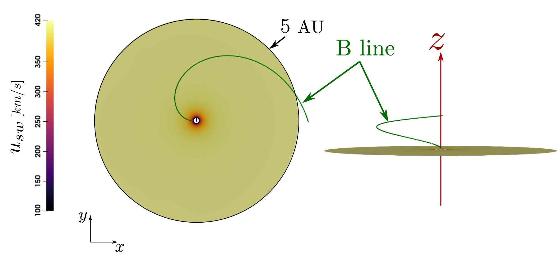
Figure 1: Inner region of the MHD simulation : top and side view of the ecliptic plane once the steady state has been reached. A magnetic field line entering the domain at $24^{\circ}$ latitude is also shown.

The dipole and the plasma between the Sun and the inner boundary of the simulation domain are assumed to rotate rigidly. Consequently, the components of the fluid velocity tangential to the surface are given by $\Omega\hat{z}\times{\bf r}$, where $\Omega=2\pi/(30{\>\rm days})$ is the Sun’s angular rotation velocity. The radial component of the fluid velocity obeys to a free stream condition $\partial u_{r}/\partial r=0$ while the plasma temperature and the mass density are kept at $2{\rm\ MK}$ and $1.2\times 10^{-20}{\rm\ kg/m^{3}}$, respectively. At the outer boundary, we adopt $\partial/\partial r=0$ for all quantities. As for the planetary field in [4], we treat the dipolar field of the Sun as a background field. With this set-up the wind emanating from the inner boundary rapidly reaches a steady and supersonic radial speed of the order 400 km/s with the magnetic field lines spiraling away from the inner boundary as shown in Fig. 1. The density and magnetic field in the simulated wind are smaller but still representative of the real wind, as illustrated in Table 1 where we also report the magnetic field variation scale $L_{\rm B}\equiv|\partial\ln B/\partial s|^{-1}$ ($s$ is the distance along the magnetic field line).

Table 1: Wind parameters at $r=1\>{\rm AU}$ on the field line of Figure 1

Magnetic field strength $B$	$0.89\>{\rm nT}$
Wind speed $u$	$418\>{\rm km/s}$
Sound speed $c_{\rm s}=(\tfrac{5}{3}p/\varrho)^{1/2}$	$48.2\>{\rm km/s}$
Alfvén speed $c_{\rm A}=(B^{2}/\mu_{0}\varrho)^{1/2}$	$71.9\>{\rm km/s}$
Plasma beta $\beta=2\mu_{0}p/B^{2}$	$0.54$
Magnetic scale length $L_{\rm B}\equiv|\partial\ln B/\partial s|^{-1}$	$0.93\>{\rm AU}$

II.2 Particles dynamics : Guiding Center Approximation

In the Guiding Center Approximation (GCA), the relativistic motion of a test particle of rest mass $m$ and electric charge $q$ is described by the following set of equations [5]

$$\frac{\mathrm{d}\mathbf{R}}{\mathrm{d}t} = v_{\|}\mathbf{b}+\mathbf{v}_{\rm E}+\frac{\gamma m}{qB}\mathbf{b}\times\left[\frac{\mu}{\gamma^{2}m}\nabla B+\frac{v_{\|}}{\gamma}E_{\|}\mathbf{v}_{\rm E}+v_{\|}^{2}\left(\mathbf{b}\cdot\nabla\right)\mathbf{b}\right.$$ (1)

$$+ \left.\vphantom{\frac{1}{2}}v_{\|}(\left(\mathbf{v}_{\rm E}\cdot\nabla\right)\mathbf{b}+\left(\mathbf{b}\cdot\nabla\right)\mathbf{v}_{\rm E})+\left(\mathbf{v}_{\rm E}\cdot\nabla\right)\mathbf{v}_{\rm E}\right]$$

$$\frac{\mathrm{d}(\gamma v_{\|})}{\mathrm{d}t} = \frac{q}{m}E_{\|}-\frac{\mu}{\gamma m}\mathbf{b}\cdot\nabla B+\gamma\mathbf{v}_{\rm E}\cdot\left[v_{\|}\left(\mathbf{b}\cdot\nabla\right)\mathbf{b}+\left(\mathbf{v}_{\rm E}\cdot\nabla\right)\mathbf{b}\right].$$ (2)

$$\frac{\mathrm{d}\mu}{\mathrm{d}t} = 0$$ (3)

In the above equations, the subscripts $\parallel$ and $\perp$ indicate projections parallel and perpendicular with respect to $\mathbf{B}$. $\mathbf{R}$ is the particle’s guiding center position, ${\bf v}$ its velocity, $m$ its rest mass, $\gamma\equiv 1/\sqrt{1-v^{2}/c^{2}}$ its Lorentz factor (with $c$ the speed of light), $\mu\equiv\tfrac{1}{2}m\gamma^{2}v_{\perp}^{2}/B$ its magnetic moment, $\mathbf{v}_{\rm E}\equiv\mathbf{E}\times\mathbf{b}/B$ the E-cross-B drift velocity, where $\mathbf{b}\equiv{\bf B}/B$ is the unit vector along $\bf B$. In ideal MHD, $\mathbf{E}=-\mathbf{u}\times\mathbf{B}$. However, since the electric field enters into the system of MHD equations through $\partial{\bf B}/\partial t=\nabla\times{\bf E}$, an additional irrotational component of $\bf E$ affects the motion of the test particles but not the MHD flow. Even though $\nabla p/n$ is not irrotational in general, we adopt the non-ideal two fluid Ohm’s law $\mathbf{E}=-\mathbf{u}\times\mathbf{B}-\nabla p_{\rm e}/(en_{\rm e})$, where $e$ is the positive elementary charge, and $p_{\rm e}$ and $n_{\rm e}$ the electron pressure and the electron number density, respectively. We assume a fully ionized electron-proton plasma so that we can write $\nabla p_{\rm e}/n_{\rm e}=2\kappa(1+\kappa)^{-1}\nabla p/n$ where $\kappa\equiv T_{\rm e}/T_{\rm p}$ is the electron to proton temperature ratio which we shall set to $\kappa=1$. Barotropic flows with $p=p(\varrho)$ are the most general flows for which $\nabla\times(\nabla p/n)=0$ holds. In the wind simulation, $p$ and $\varrho=n\overline{m}$ ($\overline{m}$ is the mean mass of the particles in the fluid) are constants on the inner boundary. Since $p/\varrho^{\gamma}$ is conserved along streamlines, and since all fluid parcels in the simulation domain emanate from the inner boundary, $p/p_{0}=(\varrho/\varrho_{0})^{\gamma}$ in the whole simulation domain. The wind simulation being compatible with the non-ideal Ohm’s law, we use it to evaluate the electric field in the simulated wind. We shall however recall, that in the solar wind, the large scale electrostatic potential between the corona and $r=1\>{\rm AU}$ is of the order of a few hundreds of Volts only, and of some relevance for particles at $\lesssim 1\>{\rm keV}$. As a final remark, we note, that the above GCA equations are for non-relativistic flows with $|\mathbf{u}|\ll c$, a condition largely satisfied in the solar wind (relativistic flows are considered in [5]).

Test particles are initialized within the MHD simulation grid of the solar wind and evolve with the simulated fields and advanced in time according to the GCA equations (1)-(3). We use a trilinear interpolation from the MHD grid to evaluate the fields at the particle position and, the $3^{rd}$ order prediction-correction time integration scheme by Mignone et al. [6] which we shortly outline hereafter. By noting $\mathbf{X}\equiv\{\mathbf{R},{\color[rgb]{0,0,0}\gamma v_{\|}}\}$ and by posing $\mathbf{F}$ to be the right-hand-side terms of the equations (1)-(2), we can write the GCA equations as

$$\frac{\mathrm{d}\mathbf{X}}{\mathrm{dt}}=\mathbf{F}{\color[rgb]{0,0,0}\left({\bf X}\right)}.$$ (4)

The time integration of (4), to advance the particle from time level $t^{n}$ to $t^{n+1}=t^{n}+\Delta t^{n}$ is done by a predictor step followed by a corrector step:

$$\mathbf{X}^{*} = \mathbf{X}^{n}+\Delta t^{n}\left[\left(1+\frac{\tau^{n}}{2}\right)\mathbf{F}^{n}-\frac{\tau^{n}}{2}\mathbf{F}^{n-1}\right]+\mathcal{O}(\Delta t^{3})$$ (5)

$$\mathbf{X}^{n+1} = {\color[rgb]{0,0,0}\mathbf{X}^{n}}+\frac{\Delta t^{n}}{6(1+\tau^{n})}\left[3\left(\mathbf{F}^{n}+\mathbf{F}^{*}\right)+4\tau^{n}\left(\mathbf{F}^{n}+\frac{\mathbf{F}^{*}}{2}\right)\right.+(\tau^{n})^{2}(\mathbf{F}^{n}-\mathbf{F}^{n-1})\left.\vphantom{\frac{1}{2}}\right]+\mathcal{O}(\Delta t^{4})$$ (6)

where $\mathbf{X}^{n}=\mathbf{X}(t^{n})$, $\mathbf{F}^{n}=\mathbf{F}({\bf X}^{n})$ and $\tau^{n}\equiv\Delta t^{n}/\Delta t^{n-1}$. We point to the fact that the factor 3 in (6) is missing in the corresponding equation (15) of [6]. At start, at $t=0$, and after a collision, the unknown quantities at $t^{n-1}$ are determined with a simple backward Euler step : $\mathbf{X}^{n-1}=\mathbf{X}^{n}-\Delta t^{n}\mathbf{F}^{n}$.

II.3 Pitch angle scattering

In the solar wind, the mean free path for Coulomb collisions is of the order of 1 AU for thermal ions and electrons. Since it grows as $v^{4}$, Coulomb collisions are completely ineffective for energetic particles. However, energetic particles are diffused in velocity space by turbulent fluctuations of the wind’s electromagnetic field [7]. The diffusion is generally supposed to occur through the accumulation of small deviations, which can be simulated numerically by applying a Fokker-Planck diffusion operator to an initial distribution of particles (see e.g. [8]). We adopt a different approach by letting test particles undergo hard-sphere type collisions. In practice, for a particle having covered a distance $\Delta s=\int_{0}^{\Delta t}v_{\parallel}dt$ during the time step $\Delta t$, and given a mean free path $\lambda_{\|}$, the collision probability

$$p(\Delta s)=1-\exp(-\Delta s/\lambda_{\parallel}).$$ (7)

At each time step a random number $a$ is generated in the interval $[0,1]$. If $a<p(\Delta s)$ the particle undergoes an elastic collision (in the Sun inertial frame). In the case of a collision, the post collision angle $\alpha$ between the particle’s velocity vector ${\bf v}$ and the magnetic field $\bf B$ is selected according to

$$\alpha=\arccos(1-2a),\;\text{{\hbox{a}}: random number}\in[0,1].$$ (8)

III Preliminary results

We inject $10^{5}$ monoenergetic electrons with $81\>{\rm keV}$ energy and $\mu=0$ at $r=0.279\>{\rm AU}$ on the magnetic field line shown in figure 1. We set $\lambda_{\parallel}=0.5\;{\rm AU}$ and adopt a constant $\Delta t=5.4\>{\rm s}$ to integrate the GCA equations with the scheme (5)-(6) over a total duration $t_{\rm max}=41.7\>{\rm h}$. Particles crossing the inner domain boundary at $r=0.139\>{\rm AU}$ or the surface $r=5\>{\rm AU}$ (the subdomain in Fig. 1) are re-injected at the same initial position (in the inertial frame) and with the same initial velocity. At $t=7\>{\rm h}$, a statistically steady distribution of particles is obtained, so that in the following we only consider particles living in the era from $t=7\>{\rm h}$ to $t=t_{\rm max}$. From an order of magnitude estimate of the terms in equation (2) it is clear that for 81 keV electrons, energy changes are essentially due to the field curvature term. Assuming time steadiness, we can then rewrite (2) as

$$\frac{d\mathcal{E}}{dt}\simeq m\gamma v_{\parallel}^{2}\;{\bf v}_{\rm E}\cdot({\bf b}\cdot\nabla{\bf b})$$ (9)

where $\mathcal{E}=(\gamma-1)mc^{2}$ is the particle’s relativistic kinetic energy. In the present configuration, ${\bf v}_{\rm E}$ is oriented opposite to the curvature vector ${\bf b}\cdot\nabla{\bf b}$ so that (9) describes a systematic loss of energy regardless of the direction the particle is moving towards (also see Fig. 2 in [1]). For all particles, the loss rate computed from the right-hand-side of (9) is reported in the bottom panel of Figure 2. For the given wind conditions, the maximum loss rate occurs at $r=1.24\>{\rm AU}$. For increasing $r$, the loss rate drops because of the field lines’ increasing curvature. For decreasing $r$, the loss rate drops because of the decreasing ${\bf v}_{\rm E}$, as the fluid velocity and the magnetic field tend to align when approaching the inner boundary.

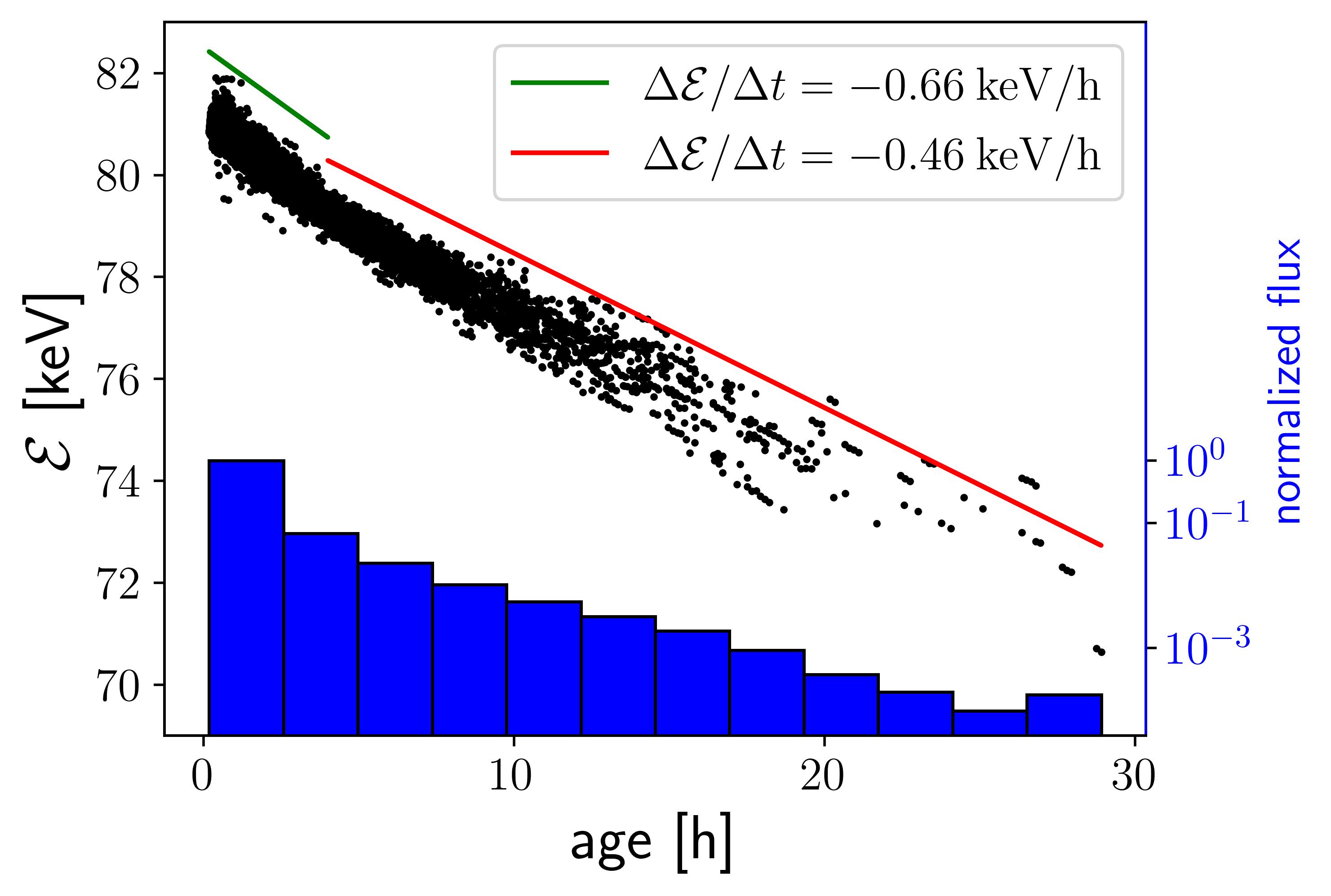
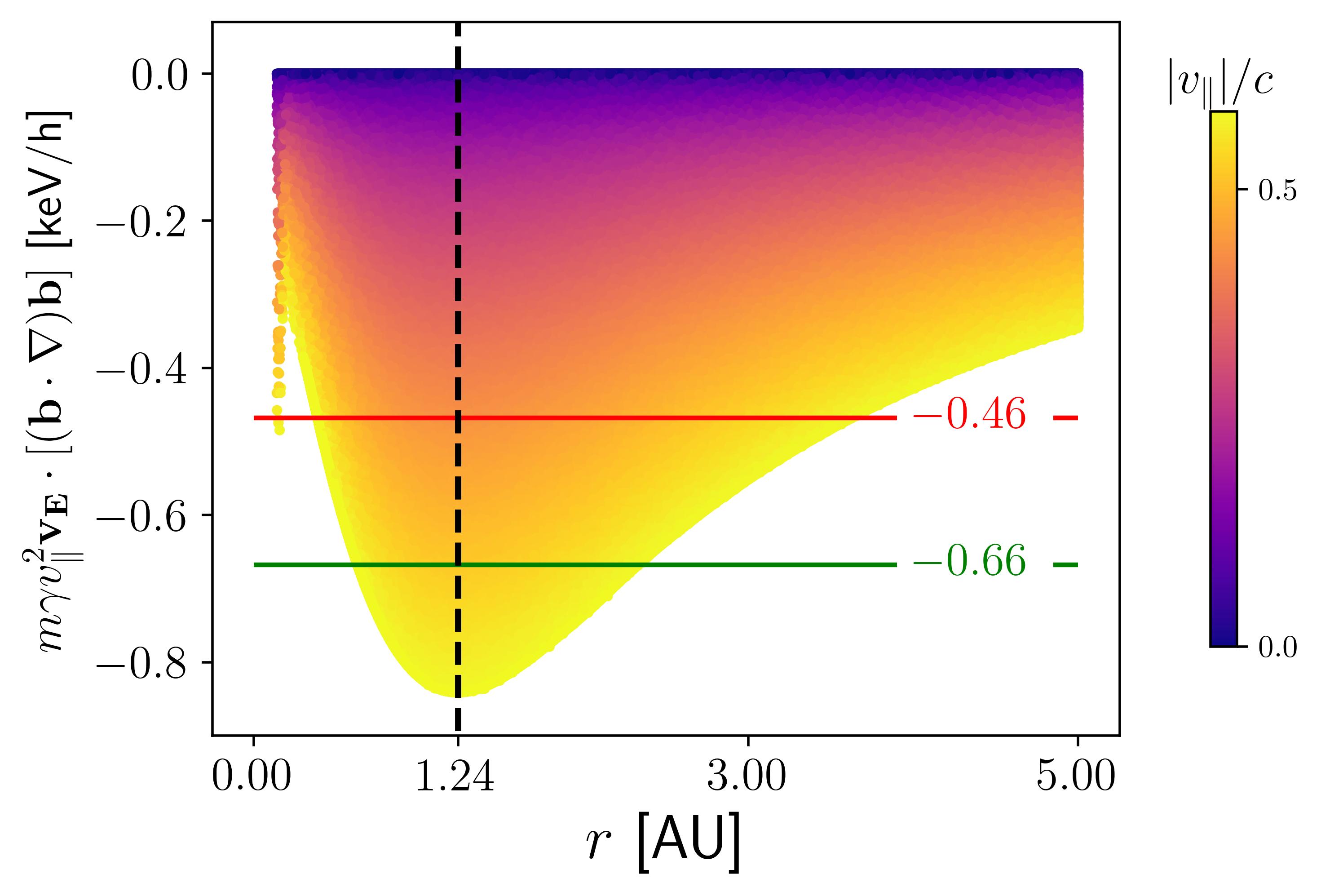
Figure 2: Top: Energy vs age for electrons near $r=1$ AU. Linear fits of the decay rate for young (age < 4 h) and old (age$\geq$ 4 h) are given. Also plotted is the normalized age distribution. Bottom: Energy loss rate as function of heliocentric distance $r$ from the right-hand-side of equation (9).

Assuming continuous injection, the loss of kinetic energy as a function of age ($=$ time since injection) for particles in the range $r\in[0.9,1.1]\>{\rm AU}$ is monitored in the left panel of Fig. 2. In the case of a transient injection, for example due to a solar event, the flux of 81 keV electrons at 1 AU reaches its peak after $\sim 10\>{\rm min}$ from injection. As the peak intensity decreases on a timescale of the order of 10 to 20 minutes, only electrons aged less than 20 min are representative of the peak distribution. The pitch-angle distribution of these young electrons is plotted in the left panel of Fig. 3 and compared with measurements from the Wind spacecraft during a 9 minutes interval following the peak of the 20th October 2002 solar event (adapted from Fig. 9 of Dröge et al. [9] for particles in the range 49 to 81 keV). In order to remove the dependence on the initial condition (in our case $\mu=0$) only electrons having undergone at least one collision have been retained to generate the distributions in Fig. 3. This is the reason for the rapid drop of the ${\rm age}<20\>{\rm min}$ distribution for $\alpha\rightarrow 180^{\circ}$ but could also be the reason for the differences at smaller values of $\alpha$. Not surprisingly, the inset shows that the angular distribution of young electrons is more field aligned compared to the steady state distribution including electrons of all ages.

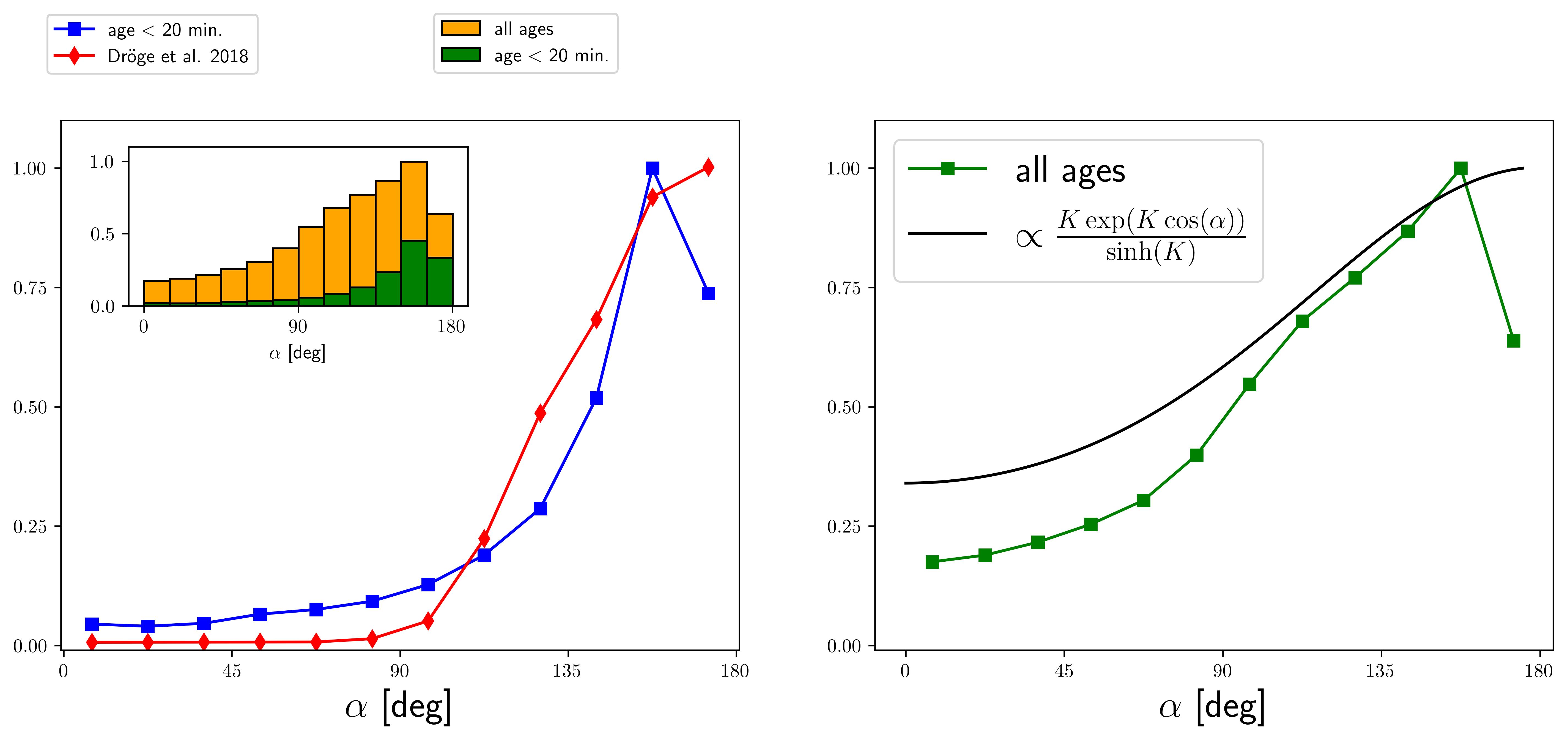
Figure 3: Normalized pitch-angle distribution for 81 keV electrons. Left: particles aged less than 20 min compared to electron data from the Wind 3DP SST instrument for the 20th October 2002 14:30 solar energetic particle event (adapted from [9]). Right: all age particles (steady state distribution) compared to Zaslavsky’s expression for a constant Knudsen ${\rm K}=\lambda_{\parallel}/L_{\rm B}=0.54$.

The pitch angle distribution for the electrons of all ages is also shown in the right panel of Fig. 3 where it is compared to the distribution ${\rm K}\exp({\rm K}\cos\alpha)/(2\sinh({\rm K}))$ obtained by Zaslavsky from a Fokker-Planck type equation (cf this conference) in the limit of a spatially constant and small Knudsen number ${\rm K}=\lambda_{\|}/L_{\rm B}$. Differences compared to Dröge et al. [9] (left) and to Zaslavsky (right) can be attributed to several factors. Besides the choice of the initial condition $\mu=0$ and the position of the injection, we use hard sphere type collisions which is probably a less realistic model, especially in the case of ${\rm K}\gtrsim 1$, than the accumulation of small angle deviations adopted by other authors ([8, 9]).

IV Conclusion

The trajectories and the distribution of energetic test electrons propagating in the field of a simulated solar wind have been obtained by integrating the relativistic GCA equations of motion using a $\mathcal{O}(\Delta t^{3})$ predictor-corrector algorithm from [6].

In our case study, we simulate $81\>{\rm keV}$ test electrons continuously injected into a steady magnetized solar wind at a heliocentric distance $r=0.139\>{\rm AU}$ and $24^{\circ}$ latitude. For a parallel mean free path $\lambda_{\parallel}=0.5\>{\rm AU}$, the particle flux observed near $r=1\>{\rm AU}$ some $30\>{\rm h}$ after injection is reduced by $\sim 10^{4}$ with respect to the initial flux (see top of Fig. 2). For these electrons, an energy loss of roughly $10\%$ is observed, quasi-exclusively due to the curvature of the magnetic field as expressed by equation (9). In our case study, the maximum loss rate occurs near $r=1.24\>{\rm AU}$ (see Fig. 2). For $\lambda_{\parallel}=0.5\>{\rm AU}$, the pitch angle distribution of old electrons (age $\gtrsim 20$ min), which are confined near $r=1\>{\rm AU}$ by both collisions and magnetic mirroring, differs significantly from that of young electrons aged $\lesssim 20$ min. The latter, having suffered at most one or two reflections by collisions or magnetic mirroring, are representative of the distribution of the particles observed at the time of maximum flux after a solar event (cf left panel of Fig. 3) confirming that $\lambda_{\parallel}=\mathcal{O}(1\>{\rm AU})$ for $\mathcal{O}(10^{5}\>{\rm eV})$ electrons [2, 9].

In the case of continuous injection over a time period of hours, the non-negligible contribution from old electrons (age $\gtrsim$ 20 min) makes the pitch angle distribution flatter (cf right panel of Fig. 3).