Enhancing Adversarial Training with Prior Knowledge Distillation for Robust Image Compression

Abstract

Deep neural network-based image compression (NIC) has achieved excellent performance, but NIC method models have been shown to be susceptible to backdoor attacks. Adversarial training has been validated in image compression models as a common method to enhance model robustness. However, the improvement effect of adversarial training on model robustness is limited. In this paper, we propose a prior knowledge-guided adversarial training framework for image compression models. Specifically, first, we propose a gradient regularization constraint for training robust teacher models. Subsequently, we design a knowledge distillation-based strategy to generate a priori knowledge from the teacher model to the student model for guiding adversarial training. Experimental results show that our method improves the reconstruction quality by about 9dB when the Kodak dataset is elected as the backdoor attack object for psnr attack. Compared with Ma2023[1], our method has a 5dB higher PSNR output at high bitrate points.

Index Terms—  Image Compression, Robustness, Adversarial Training, Gradient Regularization, Prior Knowledge

1 Introduction

Deep learning has undergone extensive research in the field of image compression[2, 3, 4, 5, 6, 7]. In terms of rate-distortion performance, the performance of deep learning models has surpassed that of traditional methods such as JPEG[8], JPEG2000[9], BPG[10], and even the recent Versatile Video Coding (VVC)[11]. However, as deep learning-based image compression models are applied in practice, considering the sensitivity of deep neural networks to minor input perturbations, the robustness of these models against adversarial perturbations has become an essential and unavoidable concern.

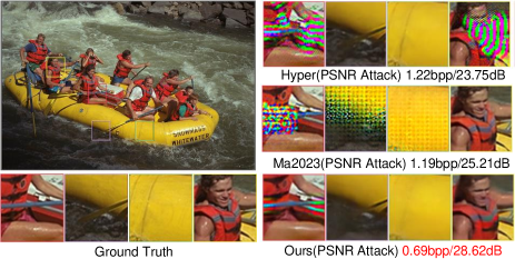
Fig. 1: Performance of the original model, Ma2023[1], and our model under attack. Our model outperforms both Hyper model and Ma2023[1] model in terms of both bpp and psnr performance.

Since the image compression models used in practice are mostly publicly accessible, in this paper, we assume that attackers can access all parameters of the neural network compression model. Therefore, the attacks mentioned in this paper are all considered white-box attacks.

The concept of adversarial samples was first introduced by Szegedy[12], which unveiled the sensitivity of deep neural networks to input perturbations. Following this, Goodfellow introduced an efficient attack method called the Fast Gradient Sign Method (FGSM) by utilizing gradient signs[13]. Kurakin enhances the attack capability by breaking down the larger step in the FGSM iteration into many smaller steps[14]. Madry proposed the Projected Gradient Descent (PGD) method, which increases attack success rates through multiple iterations[15]. In the context of image compression tasks, Ma introduced a trainable noise as an input perturbation[1], using this noise during training to update the model’s input and generate highly potent adversarial samples. Liu leveraged the PGD method to efficiently attack the model’s bpp (bits per pixel) parameter[16]. We have enhanced the techniques proposed in [1], introducing two attack methods tailored for image compression: psnr attack and bpp attack.

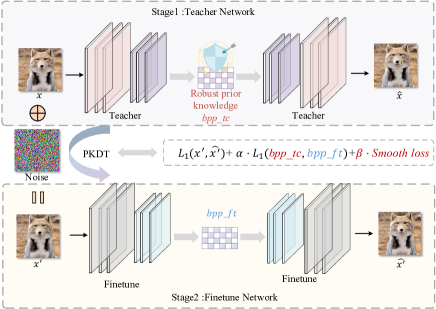
Fig. 2: Prior knowledge-guided adversarial training framework for image compression models. In the first stage, gradient regularization constraints are used to train robust teacher models. Subsequently, in the second stage, a prior knowledge distillation transfer strategy (PKDT) is used to transfer prior knowledge generated by the teacher model to the finetune model to guide adversarial training.

Adversarial Training[17, 18], serves as the most effective method to enhance a model’s resilience against adversarial attacks. The core idea of this technique is to introduce adversarial samples and use them as supplementary data alongside the original dataset for model training. The training process can be framed as a min-max problem, where the maximization problem involves generating adversarial samples with strong attack capabilities and the minimization problem focuses on training the model to minimize the output loss for these adversarial samples. However, applying adversarial training directly to image compression tasks resulted in relatively minor improvements in model robustness. To further enhance the model’s robustness, we introduce prior knowledge into the adversarial training process of the model through a distillation framework[19]. Contributions of this paper are summarized as follows:

$\bullet$ We propose a $smooth\_loss$ to train the teacher model and utilize this teacher model to generate strong robustness-oriented prior knowledge.

$\bullet$ We propose a distillation framework to transfer prior knowledge and use this knowledge to guide the model’s adversarial training.

$\bullet$ Extensive experiments demonstrate that our proposed method significantly enhances the model’s robustness. In the Kodak dataset, our method can achieve a maximum robustness improvement of up to 23% against psnr attack.

Algorithm 1 Adversarial Training with Prior Knowledge

1:Pre-trained model $M\_pre$, Dataset $D$, Training epoch $N$, psnr attack iterations $N_{p}$, bpp attack iterations $N_{b}$

2:Finetune model $M\_ft$

3:Stage I: Training a robustness teacher model $M\_tc$

4:Let $M\_tc=M\_pre$

5:for $i<N$ do

6:     $\vec{x}=Random\_Sample(D,batchsize=16)$

7:     $smooth\_loss=\frac{{\partial{\rm{bpp}}\_main}}{{\partial x}}+\frac{{\partial y}}{{\partial x}}$

8:     $loss=RD\_loss+\alpha\cdot smooth\_loss$

9:     updating the parameters of model $M\_tc$ by $loss$

10:end for

11:return teacher model $M\_tc$

12:Stage II: Finetune network, adversarial training with prior knowledge

13:Let $M\_ft=M\_pre$

14:for $i<N$ do

15:     $\vec{x}_{ori}=[x_{1},x_{2},x_{3}]$

16:$\quad\quad\quad=Random\_Sample(D,batchsize=3)$

17:     Generate adversarial sample $\acute{x_{1}}$ through psnr attack

18:   on $x_{1}$ with $N_{p}=200$, generate adversarial sample

19:   $\acute{x_{2}}$ through bpp attack on $x_{2}$ with $N_{b}=100$

20:     $\vec{x}_{new}=[{x}^{\prime}_{1},{x}^{\prime}_{2},x_{3}]$

21:     Input $\vec{x}_{ori}$ into model $M\_tc$ to obtain $bpp\_tc$

22:   Input $\vec{x}_{new}$ into model $M\_ft$ to obtain $bpp\_ft$

23:     $D\_loss={\left\|{{{\vec{x}}_{new}}-M\_ft({{\vec{x}}_{new}})}\right\|_{1}}$

24:     $R\_loss={\left\|{bpp\_tc-bpp\_ft}\right\|_{1}}$

25:     $smooth\_loss=\frac{{\partial{\rm{bpp}}\_main}}{{\partial x}}+\frac{{\partial y}}{{\partial x}}$

26:     $loss=D\_loss+\alpha\cdot R\_loss+\beta\cdot smooth\_loss$

27:     updating the parameters of model $M\_ft$ by $loss$

28:end for

2 Method

Our method effectively improves the model’s robustness by introducing a distillation framework for transferring prior knowledge. The framework of our model is illustrated in Fig.2 and consists of two components: a teacher network and a finetune network. The teacher network provides the prior knowledge necessary for training the finetune network. A gradient regularization term be used to train the teacher network, enabling it to generate prior knowledge with robustness-related information. The finetune network involves using prior knowledge generated by the teacher model to guide adversarial training. Since the $psnr$ error caused by attacks is relatively large, using $psnr$ as prior knowledge would make the adversarial training process difficult to converge. At the same time, the error of $bpp$ is very small, so we choose $bpp$ as the prior knowledge.

2.1 Stage I: Training a Robustness Teacher

Gradient regularization has been demonstrated as an effective method for improving model robustness[20, 21]. However, due to the presence of two performance metrics for the image compression task, we have designed two gradient constraint terms. Regarding the $bpp$ term, we observed that the changes in $bpp$ after the sample is attacked are mainly manifested in the $bpp$ during the analysis transformation process, which we refer to as $bpp\_main$. Therefore, the constraint term is formulated as $\partial{\rm{bpp}}\_main/\partial x$. For the $psnr$ term, we also utilize the gradient of $y$ with respect to $x$ after the analysis transformation as another constraint. Therefore, the constraint term for gradient smoothness is formulated as:

$$smooth\_loss=\underbrace{\frac{{\partial{\rm{bpp}}\_main}}{{\partial x}}}_{bpp\ constrain}+\underbrace{\frac{{\partial y}}{{\partial x}}}_{psnr\ constrain}$$ (1)

Then the overall training loss of the model is:

$$loss=RD\_loss+smooth\_loss$$ (2)

where $RD\_loss$ is the rate-distortion loss function of the pre-trained model, and $RD\_loss=R+\lambda D$, Distortion term $D$ is measured by peak signal-to-noise ratio (PSNR) between original images and reconstructed images, $R$ is the bit rate, $\lambda$ is hyper parameter to control the trade-off between rate and distortion. Through training, we obtain the teacher model, denoted as gradient model.

2.2 Stage II: Transferring Prior Knowledge

We transfer prior knowledge from the teacher network to the finetune network through a distillation framework. The prior knowledge specifically refers to the $bpp$ generated by input samples into the teacher model, denoted as $bpp\_tc$, We assume the input sample as $x$, and the reconstructed output from the sample input into the finetuned model as $\hat{x}$, with $bpp$ as $bpp\_ft$. The loss for training the finetune network consists of three components. First is the reconstruction error part:

$$D\_loss=\left\|x-\hat{x}\right\|_{1}$$ (3)

Secondly, there is the introduction of prior knowledge:

$$R\_loss=\left\|bpp\_tc-bpp\_ft\right\|_{1}$$ (4)

Lastly, the $smooth\_loss$ in Equation 2. Then the overall training loss of the model is:

$$loss=D\_loss+\alpha\cdot R\_loss+\beta\cdot smooth\_loss$$ (5)

The entire training process is depicted as Algorithm 1.

2.3 Attack Method

The image compression task involves two evaluation metrics, $psnr$ (Peak Signal-to-Noise Ratio) and $bpp$ (Bits Per Pixel), which directly impact the model’s compression performance. Therefore, we conduct attacks on these two metrics separately. When attacking $psnr$, we ensure that $bpp$ remains almost unchanged to simulate a real-world scenario where image transmission efficiency remains constant, but image decompression quality significantly deteriorates. Conversely, when attacking $bpp$, we ensure that $psnr$ remains almost unchanged to simulate a situation in the real world where image decompression quality remains constant, but transmission efficiency experiences a significant drop.

Assuming the input image is $x$, noise is $n$, adversarial samples $x^{\ast}=x+n$. The input image and the adversarial sample are both reconstructed to $\hat{x}$ and $\hat{x}^{\ast}$, simultaneously, the bit rates are $bpp\_ori$ and $bpp$, respectively. We improved the approach outlined in [1] by modifying the loss function to:

$$arg\min_{n}L_{d}=\left\{\begin{matrix}\left\|n\right\|_{2}+bpp\_error\quad\quad\left\|n\right\|_{2}^{2}\geq\epsilon\\ 1-\left\|x-\hat{x}^{\ast}\right\|_{2}^{2}\quad\quad\ \ \ \ \ \ \left\|n\right\|_{2}^{2}<\epsilon\end{matrix}\right.$$ (6)

$$arg\min_{n}L_{d}=\left\{\begin{matrix}\left\|n\right\|_{2}+psnr\_error\quad\left\|n\right\|_{2}^{2}\geq\epsilon\\ -bpp\quad\quad\quad\quad\quad\quad\quad\left\|n\right\|_{2}^{2}<\epsilon\end{matrix}\right.$$ (7)

where $\epsilon$ is the $l_{2}$ threshold of the input noise, $bpp\_error=\left\|bpp-bpp\_ori\right\|_{1}$, $psnr\_error=\left\|\left\|x-\hat{x}^{\ast}\right\|_{2}^{2}-\left\|x-\hat{x}\right\|_{2}^{2}\right\|_{1}$. Then implementing psnr attack through training Equation 6, and implementing bpp attack through training Equation 7.

3 Experiment

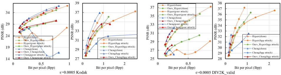
Fig. 3: R-D performance of the model under different attack scenarios. The two graphs on the left illustrate the robustness performance of our method applied to the Hyper and Cheng models using the Kodak test dataset. The first graph on the left pertains to psnr attack, while the second one is related to bpp attack, with the attack iterations $N_{p}=N_{b}=1000$. The two graphs on the right are based on the DIV2K valid dataset, with the attack iterations $N_{p}=N_{b}=500$. It’s worth noting that in the second graph on the left, the last two data points on curve Ours_Cheng(bpp attack) have bpp exceeding 9.

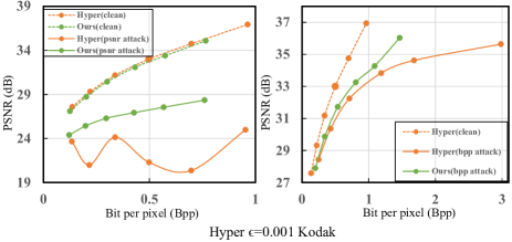
Fig. 4: R-D performance of the model under other $\epsilon$

$A.$ Experiment Setup

Datasets. The training dataset includes CLIC and DIV2K. Two datasets are used for testing, including Kodak dataset with 24 images at a size of 768×512, DIV2K valid dataset with 100 high-quality images.

Training details. We train each model for 100 epochs with Adam optimizer. For the pre-train model, the learning rate is initially set to $10^{-4}$ and then halved every 25 epochs after the initial 50 epochs. For the gradient model and ours finetune model the learning rate is initially set to $5\times 10^{-5}$, and then halved every 25 epochs after the initial 25 epochs. The pre-trained model is trained using the CLIC dataset. The gradient model and our fine-tuned model are trained using the DIVK dataset, more importantly, both of them are fine-tuned based on the pre-trained model. In the adversarial training process we proposed, the number of iterations for psnr attack $N_{p}$ is set to 200, while for bpp attack, iteration counts $N_{b}$ is set to 100, and $\epsilon=0.0005$.
$B.$ Results and Comparison

We tested two original models, Hyper[3] and Cheng[6], as well as the finetuned models obtained using our method. We evaluated these models on various test datasets and under different attack methods to obtain results. Fig.3 shows the performance comparison of our model in different scenarios. It can be observed that when our method is applied to different models, there is a noticeable enhancement in robustness. Especially for models with large parameter sizes like Cheng the improvement in robustness is more pronounced compared to the Hyper model. Additionally, we can see that our method effectively enhances model robustness in both low-resolution and high-resolution test datasets. Fig.4 illustrates the robustness performance of our method concerning different noise thresholds for $\epsilon=0.001$. It can be observed that the model’s robustness is significantly enhanced when compared to smaller noise thresholds $\epsilon=0.0005$. Particularly, in the case of bpp attack, the robustness improvement can reach up to $23\%$. Table.1 contains the data points for the low bitrate scenario shown in Fig.3, leftmost graph. It can be observed that the robustness improvement brought by our method is similarly higher than that of the gradient model, which is training with stage I.

Table 1: R-D performance of model

model	clean		psnr attack		bpp attack
	bpp	psnr	bpp	psnr	bpp	psnr
Hyper	0.4978	33	0.498	22.3502	0.9161	33.7702
Ours w/o Stage II	0.4322	32.2592	0.4309	25.9039	0.7225	33.1432
Ours	0.4323	32.0802	0.4286	28.4039	0.6822	32.9933

Adversarial training can potentially lead to a decrease in the model’s generalization ability, resulting in less improvement in robustness against other attack methods. However, we compared our approach with the attack method mentioned in Ma2023. The results of the comparison can be seen in Fig.5. It is evident that for adversarial samples where we did not undergo adversarial training, our method still exhibits better robustness.

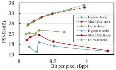
Fig. 5: R-D performance compared with Ma2023

$C.$ Ablation Experiments

We demonstrate the optimality of our method under the same training parameter conditions in Table.2. The second row represents the most effective method used in Algorithm 1. The third row represents the results obtained by training without the $smooth\_loss$ term in the stage II. Analogously, the results in the last two rows correspond to the removal of $\partial y/\partial x$ and $\partial{\rm{bpp}}\_main/\partial x$ in stage II, respectively. Test dataset is Kodak with iteration counts $N_{p}=400$, $N_{b}=200$, and noise threshold $\epsilon=0.0005$. From the results, we can observe that removing any of the constraint terms deteriorates the model’s robustness. Additionally, we have noticed that the impact on robustness is relatively small. This further validates that in our proposed method, the most significant improvement in model robustness is achieved through the introduction of prior knowledge.

Table 2: Results of the ablation experiments

model	clean		psnr attack		bpp attack
	bpp	psnr	bpp	psnr	bpp	psnr
best	0.4323	32.0802	0.4273	28.6556	0.6953	33.0194
best w/o
$smooth\_loss$	0.4358	32.1936	0.4328	28.4497	0.7214	33.0731
best w/o
$\partial y/\partial x$	0.4355	32.1549	0.4301	28.5293	0.7075	33.031
best w/o
$\partial{\rm{bpp}}\_main/\partial x$	0.4332	32.1463	0.4279	28.6224	0.7083	33.093

4 conclusion

In this paper, we propose a method of training the teacher model using gradient regularization and use the prior knowledge generated by this teacher model to guide the entire process of adversarial training. Experimental results demonstrate that our approach can effectively improve the robustness of the model. This is especially effective when dealing with large-parameter models and large noise thresholds.

References

- [1] T. Chen and Z. Ma, “Towards robust neural image compression: Adversarial attack and model finetuning,” IEEE Transactions on Circuits and Systems for Video Technology, 2023.
- [2] J. Ballé, V. Laparra, and E. P. Simoncelli, “End-to-end optimized image compression,” arXiv preprint arXiv:1611.01704, 2016.
- [3] J. Ballé, D. Minnen, S. Singh, S. J. Hwang, and N. Johnston, “Variational image compression with a scale hyperprior,” arXiv preprint arXiv:1802.01436, 2018.
- [4] D. Minnen, J. Ballé, and G. D. Toderici, “Joint autoregressive and hierarchical priors for learned image compression,” Advances in neural information processing systems, vol. 31, 2018.
- [5] D. Minnen and S. Singh, “Channel-wise autoregressive entropy models for learned image compression,” in 2020 IEEE International Conference on Image Processing (ICIP), pp. 3339–3343, IEEE, 2020.
- [6] Z. Cheng, H. Sun, M. Takeuchi, and J. Katto, “Learned image compression with discretized gaussian mixture likelihoods and attention modules,” in Proceedings of the IEEE/CVF conference on computer vision and pattern recognition, pp. 7939–7948, 2020.
- [7] Y. Bao, F. Meng, C. Li, S. Ma, Y. Tian, and Y. Liang, “Nonlinear transforms in learned image compression from a communication perspective,” IEEE Transactions on Circuits and Systems for Video Technology, vol. 33, no. 4, pp. 1922–1936, 2023.
- [8] G. K. Wallace, “The jpeg still picture compression standard,” Communications of the ACM, vol. 34, no. 4, pp. 30–44, 1991.
- [9] M. Rabbani and R. Joshi, “An overview of the jpeg 2000 still image compression standard,” Signal processing: Image communication, vol. 17, no. 1, pp. 3–48, 2002.
- [10] D. Yee, S. Soltaninejad, D. Hazarika, G. Mbuyi, R. Barnwal, and A. Basu, “Medical image compression based on region of interest using better portable graphics (bpg),” in 2017 IEEE international conference on systems, man, and cybernetics (SMC), pp. 216–221, IEEE, 2017.
- [11] B. Bross, J. Chen, J.-R. Ohm, G. J. Sullivan, and Y.-K. Wang, “Developments in international video coding standardization after avc, with an overview of versatile video coding (vvc),” Proceedings of the IEEE, vol. 109, no. 9, pp. 1463–1493, 2021.
- [12] C. Szegedy, W. Zaremba, I. Sutskever, J. Bruna, D. Erhan, I. Goodfellow, and R. Fergus, “Intriguing properties of neural networks,” arXiv preprint arXiv:1312.6199, 2013.
- [13] I. J. Goodfellow, J. Shlens, and C. Szegedy, “Explaining and harnessing adversarial examples,” arXiv preprint arXiv:1412.6572, 2014.
- [14] A. Kurakin, I. J. Goodfellow, and S. Bengio, “Adversarial examples in the physical world,” in Artificial intelligence safety and security, pp. 99–112, Chapman and Hall/CRC, 2018.
- [15] A. Madry, A. Makelov, L. Schmidt, D. Tsipras, and A. Vladu, “Towards deep learning models resistant to adversarial attacks,” arXiv preprint arXiv:1706.06083, 2017.
- [16] K. Liu, D. Wu, Y. Wang, D. Feng, B. Tan, and S. Garg, “Denial-of-service attacks on learned image compression,” arXiv preprint arXiv:2205.13253, 2022.
- [17] I. J. Goodfellow, J. Shlens, and C. Szegedy, “Explaining and harnessing adversarial examples,” arXiv preprint arXiv:1412.6572, 2014.
- [18] A. Madry, A. Makelov, L. Schmidt, D. Tsipras, and A. Vladu, “Towards deep learning models resistant to adversarial attacks,” arXiv preprint arXiv:1706.06083, 2017.
- [19] N. Papernot, P. McDaniel, X. Wu, S. Jha, and A. Swami, “Distillation as a defense to adversarial perturbations against deep neural networks,” in 2016 IEEE symposium on security and privacy (SP), pp. 582–597, IEEE, 2016.
- [20] H. Drucker and Y. Le Cun, “Improving generalization performance using double backpropagation,” IEEE transactions on neural networks, vol. 3, no. 6, pp. 991–997, 1992.
- [21] C. Finlay and A. M. Oberman, “Scaleable input gradient regularization for adversarial robustness,” Machine Learning with Applications, vol. 3, p. 100017, 2021.