Dynamic of frustrated Kuramoto oscillators with modular connections

Abstract

Synchronization and collective movement are phenomena of a highly interdisciplinary nature, with examples ranging from neuronal activations to walking pedestrians. As of today, the Kuramoto model stands as the quintessential framework for investigating synchronization phenomena, displaying a second order phase transition from disordered motion to synchronization as the coupling between oscillators increases. The model was recently extended to higher dimensions allowing for the coupling parameter to be promoted to a matrix, leading to generalized frustration and new synchronized states. This model was previously investigated in the case of all-to-all and homogeneous interactions. Here, we extend the analysis to modular graphs, which mimic the community structure presented in many real systems. We investigated, both numerically and analytically, the matrix coupled Kuramoto model with oscillators divided into two groups with distinct coupling parameters to understand in which conditions they synchronize independently or globally. We discovered a very rich and complex dynamic, including an extended region in the parameter space in which the interactions between modules were destructive, leading to a global disordered motion even tough the uncoupled dynamic presented higher levels of synchronization. Additional simulations considering synthetic modular networks were performed to assess the robustness of our findings.

I INTRODUCTION

The emergence of synchronization and its general features are of particular interest to scientists working on several subjects, such as physics, social sciences and biology [1, 2]. From neurons[3] to population dynamics and fireflies[4, 5], nature showcases several examples of synchronized and collective behavior[6]. Furthermore, recent studies show that information processing in the cerebral cortex is associated with synchronization mechanisms [7] while some brain disorders such as Alzheimer have been associated with abnormal neural sync [8]. In order to investigate the basic properties leading to synchronization, Y. Kuramoto proposed a model that became a paradigm in the field [9], being studied extensively in recent years. The original model consists of $N$ oscillators, described by internal phases $\theta_{i}$, that rotate with natural frequencies $\omega_{i}$, extracted from a given symmetric distribution $g(\omega)$. The oscillators are coupled according to the equations

$$\dot{\theta_{i}}=\omega_{i}+\dfrac{K}{N}\sum_{j=1}^{N}\operatorname{sin}(\theta_{j}-\theta_{i}),$$ (1)

in which $K$ is the coupling strength. The degree of system’s synchronization can be measured by calculating the complex order parameter $z$

$$z=pe^{i\psi}=\sum_{j=1}^{N}e^{i\theta_{j}},$$ (2)

in which $p\approx 1$ implies in coherent motion while $p\approx 0$ indicates disordered and independent oscillators. In the limit of $N\to\infty$ and all-to-all interactions, it can be shown that the system exhibits a continuous phase transition from disorder to synchronization as the control parameter $K$ increase. For small values of $K$, the oscillators move as if they were independent ($p=0$) but after a threshold $K_{c}=\dfrac{2}{\pi g(0)}$ they start to cluster together and $p$ increases as $p=\sqrt{1-K_{c}/K}$, characterizing the spontaneous synchronization.

Several extensions of the Kuramoto model have been proposed, such as oscillators embedded on networks of different topologies[10, 11], external forces [12, 13], coupling with particle motion[14, 15], frustration via matrix coupling[16, 17] and higher dimensions[18, 19]. The latter, in particular, can be visualized by interpreting the oscillators as unit vectors $\vec{\sigma_{i}}=(\cos\theta_{i},\sin\theta_{i})$[18] that rotate on the unit circle, with Eq. (1) rewritten as

$$\dfrac{d\vec{\sigma}_{i}}{dt}=\textbf{W}_{i}\vec{\sigma}_{i}+\dfrac{K}{N}\sum_{j=1}^{N}[\vec{\sigma}_{j}-(\vec{\sigma}_{i}\cdot\vec{\sigma}_{j})\vec{\sigma}_{i}],$$ (3)

where $\textbf{W}_{i}$ is an anti-symmetric matrix containing the natural frequencies $\omega_{i}$

$$\textbf{W}_{i}=\begin{pmatrix}0&\omega_{i}\\ -\omega_{i}&0\end{pmatrix}.$$ (4)

In this formulation, the order parameter can be easily calculated as

$$\vec{p}=\dfrac{1}{N}\sum_{i=1}^{N}\vec{\sigma}_{i}=(p\cos\psi,p\sin\psi).$$ (5)

The advantage of writing the equations in this format is that $\vec{\sigma_{i}}$ can be naturally extended to $D$-dimensional unit vectors, described by $D-1$ spherical angles, instead of a single phase $\theta_{i}$. The only requirement is that $\textbf{W}_{i}$ are $D$-dimensional anti-symmetric matrices.

By replacing the scalar coupling $K$ by a matrix $\mathbf{K}$, a novel and interesting generalization of the Kuramoto model was investigated in [16], with the dynamical equations acquiring the form

$$\dfrac{d\vec{\sigma}_{i}}{dt}=\textbf{W}_{i}\vec{\sigma}_{i}+\dfrac{1}{N}\sum_{j=1}^{N}[\mathbf{K}\vec{\sigma}_{j}-(\vec{\sigma}_{i}\cdot\mathbf{K}\vec{\sigma}_{j})\vec{\sigma}_{i}].$$ (6)

The matrix coupling is a form of generalized frustration, in which the vector $\vec{\sigma}_{j}$ is rotated by $\mathbf{K}$ before interacting with $\vec{\sigma}_{i}$. In this work we restrict ourselves to $D=2$. In this case, if $\mathbf{K}$ is a rotation matrix, the equations for the phases are equivalent to the Kuramoto-Sakaguchi model[20]. In general, we can write the coupling matrix as a sum of a rotation matrix $\mathbf{K}_{R}$ and a symmetric $\mathbf{K}_{S}$:

$$\textbf{K}\equiv\mathbf{K}_{R}+\mathbf{K}_{S}=K\begin{pmatrix}\cos\alpha&\sin\alpha\\ -\sin\alpha&\cos\alpha\end{pmatrix}+J\begin{pmatrix}-\cos\beta&\sin\beta\\ \sin\beta&\cos\beta\end{pmatrix}.$$ (7)

In terms of the original angular formalism this is equivalent to

$$\dot{\theta}_{i}=\omega_{i}+\sum_{j=1}^{N}\left[K\sin(\theta_{i}-\theta_{j}-\alpha)+J\sin(\theta_{i}+\theta_{j}+\beta)\right].$$ (8)

For $J\neq 0$, the system exhibits novel behaviors such as active states., i.e., a synchronized state in which the phase and module of $\vec{p}$ oscillates in time and the phase tuned, in which all oscillators lock onto the direction of the principal eigenvector of $\mathbf{K}$, breaking the rotational symmetry of the system.

This generalized frustration in the Kuramoto model was studied in the context of multidimensional substrates, all-to-all interactions and same $\mathbf{K}$ for all oscillators [16, 21, 17]. However, in real systems, the oscillators usually have an interacting neighborhood, that can be modeled as a network. A particular topology that draws attention to synchronization phenomena are the modular networks [22, 23, 24, 25]: a collection of nodes organized in groups with the property of being densely connected within the group but interacting weakly with vertices outside the module[26]. Modular networks are interesting substrates to mimic community structure presented in real systems such as neuronal[27, 28], social and biological networks[29]. Here, as a first approach to modular structures, we considered a complete graph of oscillators divided into groups $\mathcal{G}_{1}$, $\mathcal{G}_{2}$,…,$\mathcal{G}_{\Omega}$, and a set of matrices $\mathbf{K}_{sm}$ that indicates the coupling between elements of module $s$ and $m$. Direct computations with two modules show that the system displays a rich and complex dynamic. In particular, we found an extended region in the parameter space where the motion is disordered, even though the uncoupled dynamic presented higher levels of synchronization.

The remaining paper is organized as follows. In Section II, we construct the dynamical equations for the modular oscillators with matrix coupling and perform a dimensionality reduction using the Ott-Antonsen ansatz. Constraining our analysis to systems with two modules, we investigate the phase diagram of some particular cases of distinct modules in Section III. In Section IV we perform simulations on synthetic modular systems for comparative purposes. Finally, some discussions and remarks are presented in Section V.

II MODULAR MATRIX COUPLING

We extend Equation (6) to accommodate modular connections, in which the dynamical equation for an oscillator $i$ belonging to module $s=1,2,...,\Omega$ can be written as

$$\frac{d\vec{\sigma}_{i}^{s}}{dt}=\textbf{W}_{i}\vec{\sigma}_{i}^{s}+\sum_{m=1}^{\Omega}\dfrac{\eta_{m}}{N_{m}}\sum_{j=1}^{N_{m}}[\mathbf{K}_{sm}\vec{\sigma}_{j}^{m}-(\vec{\sigma}_{i}^{s}\cdot\mathbf{K}_{sm}\vec{\sigma}_{j}^{m})\vec{\sigma}_{i}^{s}],$$ (9)

in which $\eta_{m}$ is the fraction of oscillators within module $m$, $\eta_{m}=N_{m}/N$, and the matrices $\mathbf{K}_{sm}$ are parametrized by $K_{sm}$,$J_{sm}$,$\alpha_{sm}$ and $\beta_{sm}$ as in Equation (7). In addition, we define order parameters for each module

$$\vec{p}_{s}=\left(p_{s}\cos{\psi_{s}},p_{s}\sin{\psi_{s}}\right)=\dfrac{1}{N_{s}}\sum_{i=1}^{N_{s}}\vec{\sigma}_{i}^{s},$$ (10)

and for the whole system

$$\vec{p}_{T}=\left(p_{T}\cos{\psi_{T}},p_{T}\sin{\psi_{T}}\right)=\sum_{s=1}^{\Omega}\eta_{s}\vec{p}_{s}.$$ (11)

We also define the auxiliary vectors

$$\vec{q}_{sm}=\left(q_{sm}\cos{\gamma_{sm}},q_{sm}\sin{\gamma_{sm}}\right)=\dfrac{\eta_{m}}{N_{m}}\sum_{j=1}^{N_{m}}\mathbf{K}_{sm}\vec{\sigma}_{j}^{m}=\eta_{m}\mathbf{K}_{sm}\vec{p}_{m},$$ (12)

to rewrite Equation (9) in a more compact form as

$$\frac{d\vec{\sigma}_{i}^{s}}{dt}=\textbf{W}_{i}\vec{\sigma}_{i}^{s}+\sum_{m=1}^{\Omega}[\vec{q}_{sm}-(\vec{\sigma}_{i}^{s}\cdot\vec{q}_{sm})\vec{\sigma}_{i}^{s}].$$ (13)

Next, we use the Ott-Antonsen ansatz[30] to reduce the complexity of the problem and write differential equations for the order parameters $\vec{p}_{s}$ instead of individual oscillators. We start by considering the continuum limit of infinite oscillators and defining $f_{s}(\omega,\theta,t)$ as the density of oscillators belonging to module $s$ with natural frequency $\omega$ at position $\theta$ in time $t$. It satisfies the continuity equation

$$\dfrac{\partial f_{s}}{\partial t}+\dfrac{\partial(f_{s}v_{s\theta})}{\partial\theta}=0,$$ (14)

with velocity field

$$v_{s\theta}=\omega_{s}+\sum_{m=1}^{\Omega}(q_{sm}\sin(\gamma_{sm}-\theta)).$$ (15)

In terms of $f_{s}(\omega,\theta,t)$, the equations for the order parameters can be written as

$$\vec{p}_{s}(t)=\int\hat{r}(\theta)f_{s}(\omega,\theta,t)d\theta d\omega.$$ (16)

We now make use of the ansatz by expanding $f_{s}$ in Fourier series and choosing the coefficients in terms of a single complex parameter $\nu_{s}(\omega,t)$:

$$f_{s}(\omega,\theta,t)=\dfrac{g_{s}(\omega)}{2\pi}\left[1+\sum_{n=1}^{\infty}\nu_{s}^{n}e^{-in\theta}+\sum_{n=1}^{\infty}\nu_{s}^{*n}e^{in\theta}\right].$$ (17)

Inserting Equations (15) and (17) into Equation (14) and defining $u_{sm}=q_{sm}e^{i\gamma_{sm}}$ (see Eq.(12)), we obtain differential equations for parameters $\nu_{s}$:

$$\dot{\nu}_{s}=-i\omega\nu_{s}-\dfrac{1}{2}\sum_{m=1}^{\Omega}\left[u^{*}_{sm}\nu_{s}^{2}-u_{sm}\right].$$ (18)

Using Equation (12) and considering Equation (2) for each module, $z_{s}=p_{s}e^{i\psi_{s}}$, the complex numbers $u_{sm}$ can be written as

$$u_{sm}=K_{sm}\eta_{m}z_{m}e^{-i\alpha_{sm}}-J_{sm}\eta_{m}z_{m}^{*}e^{-i\beta_{sm}}.$$ (19)

Finally, the order parameters $z_{s}$ can be written as

$$z_{s}=\int f_{s}(\omega,\theta,t)e^{i\theta}d\theta d\omega=\int g_{s}(\omega)\nu_{s}(\omega)d\omega,$$ (20)

where we used Equation (17). This integral can be solved analytically if $g_{s}(\omega)$ is a Lorentzian distribution:

$$g_{s}(\omega)=\dfrac{1}{\pi}\dfrac{\Delta_{s}}{(\omega-\omega_{0s})^{2}+\Delta_{s}^{2}}.$$ (21)

In this case, the integrand has poles at $\omega=\omega_{0s}\pm i\Delta_{s}$ and the overall integral can be performed by using the residues theorem, obtaining $z_{s}=\nu_{s}(\omega_{0s}+i\Delta_{s})$. See Ref. [16] for detailed calculations. Therefore, $\nu_{s}$ can be replaced by $z_{s}$, resulting in the following differential equation

$$\dot{z}_{s}=i(\omega_{s0}+i\Delta_{s})z_{s}-\sum_{m=1}^{\Omega}\dfrac{\eta_{m}}{2}\left[\left(K_{sm}z^{*}_{m}e^{i\alpha_{sm}}-J_{sm}z_{m}e^{i\beta_{sm}}\right)z_{m}^{2}+\left(K_{sm}z_{m}e^{-i\alpha_{sm}}-J_{sm}z_{m}^{*}e^{-i\beta_{sm}}\right)\right].$$ (22)

Separating the real and imaginary parts of Equation (22), we find dynamical equations for the module and phase of the order parameter $z_{s}$ as

$$\dot{p}_{s} =-\Delta_{s}p_{s}+\sum_{m=1}^{\Omega}\dfrac{\eta_{m}p_{m}}{2}(1-p_{s}^{2})\left[K_{sm}\cos(\psi_{s}-\psi_{m}+\alpha_{sm})-J_{sm}\cos(\psi_{s}+\psi_{m}+\beta_{sm})\right],$$ (23)

$$p_{s}\dot{\psi}_{s} =\omega_{0s}p_{s}-\sum_{m=1}^{\Omega}\dfrac{\eta_{m}p_{m}}{2}(1+p_{s}^{2})\left[K_{sm}\sin(\psi_{s}-\psi_{m}+\alpha_{sm})+J_{sm}\sin(\psi_{s}+\psi_{m}+\beta_{sm})\right].$$ (24)

From now on, we will consider the particular case of two modules with same sizes. Therefore we can absorb $\eta_{m}=1/2$ into $K_{sm}$ and $J_{sm}$. The most general coupling between two modules has sixteen parameters. For sake of simplicity, we will consider that matrices $\mathbf{K}_{12}$ and $\mathbf{K}_{21}$ are identical and given by $K_{12}\mathbb{1}$. To simplify matters we set $\beta=0$ for all $\mathbf{K}$ [16]. With these assumptions, the dynamic of the system can be written as the following set of differential equations

$$\dot{p}_{1} =-\Delta_{1}p_{1}+\frac{p_{1}}{2}(1-p_{1}^{2})\left[K_{1}\operatorname{cos}\alpha_{1}-J_{1}\operatorname{cos}(2\psi_{1})\right]+\frac{p_{2}}{2}(1-p_{1}^{2})K_{12}\operatorname{cos}\xi$$ (25)

$$\dot{p}_{2} =-\Delta_{2}p_{2}+\frac{p_{2}}{2}(1-p_{2}^{2})\left[K_{2}\operatorname{cos}\alpha_{2}-J_{2}\operatorname{cos}(2\psi_{2})\right]+\frac{p_{1}}{2}(1-p_{2}^{2})K_{12}\operatorname{cos}\xi$$ (26)

$$p_{1}\dot{\psi}_{1} =+\omega_{1}p_{1}-\frac{p_{1}}{2}(1+p_{1}^{2})\left[K_{1}\operatorname{sin}\alpha_{1}-J_{1}\operatorname{sin}(2\psi_{1})\right]-\frac{p_{2}}{2}(1+p_{1}^{2})K_{12}\operatorname{sin}\xi$$ (27)

$$p_{2}\dot{\psi}_{2} =+\omega_{2}p_{2}-\frac{p_{2}}{2}(1+p_{2}^{2})\left[K_{2}\operatorname{sin}\alpha_{2}-J_{2}\operatorname{sin}(2\psi_{2})\right]+\frac{p_{1}}{2}(1+p_{2}^{2})K_{12}\operatorname{sin}\xi$$ (28)

in which $\xi=\psi_{1}-\psi_{2}$ is the phase difference among the modules.

III DYNAMIC OF DISTINCT MODULES

Despite the reduction in the number of parameters, Equations (25) to (28) are still complex and difficult to solve analytically for $J\neq 0$. In addition, the remaining seven parameters generate an enormous number of particular cases to be studied. Therefore, we will restrict ourselves to the most extreme case: module $\mathcal{G}_{1}$ acting as a Kuramoto-Sakaguchi system ($K_{1}\neq 0;\alpha_{1}\neq 0;J_{1}=0$) and module $\mathcal{G}_{2}$ with complementary parameters ($K_{2}=0;\alpha_{2}=0;J_{2}\neq 0$). In addition, both the mean and standard deviation of the natural frequency distribution, $\omega$ and $\Delta$ respectively, will be the same for $\mathcal{G}_{1}$ and $\mathcal{G}_{2}$. Finally, we set $K_{1}=10$ and $J_{2}=3$ to guarantee individual synchronization in the absence of $K_{12}$. It is important to notice that since $K_{2}=0$, module $\mathcal{G}_{2}$ will be in phase tuned state, in which $\vec{p}_{2}$ align with the principal eigenvector of $\mathbf{K}_{2}$ (which is the $\hat{y}$ direction for $\beta=0$), at least for a range of $\omega$ around zero.

With these considerations, we performed numerical integration of Equations (25) to (28) using fourth order Runge-Kutta algorithm, varying the phase-lag parameter $\alpha_{1}$ and the intermodule coupling $K_{12}$, computing the stationary time-average order parameter $\langle p_{s}\rangle$ for both individual modules ($\langle p_{1}\rangle$ and $\langle p_{2}\rangle$) and the system as a whole ($\langle p_{t}\rangle$). Figure 1 shows the average orders parameters for $\mathcal{G}_{1}$, $\mathcal{G}_{2}$ and the full system $\mathcal{G}_{1}+\mathcal{G}_{2}$ in the form of a heatmap in the $\alpha_{1}\times K_{12}$ plane. Figure 1-(a), that refers to $\mathcal{G}_{1}$, presents a transition for small $K_{12}$ at $\alpha_{1}\approx 1.37$, in accordance with the usual Kuramoto-Sakaguchi order-disorder transition, in which the solution $p_{1}=0$ becomes stable when $K\cos\alpha<2\Delta$ [31]. For larger values of $K_{12}$ this behavior changes, as the modular structure becomes fuzzy. More interestingly, we observe the appearance of a fully asynchronous region (around $K_{12}=5$ and $\alpha_{1}=1.5$), in which $\langle p\rangle\to 0$, indicating a destructive interaction between the modules, since they were partially synchronized when decoupled. Below this region both modules synchronize and above it we see chimera-like states, where $\mathcal{G}_{1}$ is largely out of sync but $\mathcal{G}_{2}$ is synchronized.

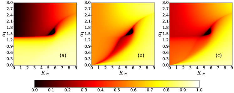
Figure 1: Heatmaps in $\alpha_{1}\times K_{12}$ parameter space showing the time averaged order parameter (a) $\langle p_{1}\rangle$; (b) $\langle p_{2}\rangle$; (c) $\langle p_{t}\rangle$; obtained via numerical integration of Equations (25) to (28) with $\omega_{0}=0$ and $\Delta=1$.

The time-averaged order parameter provides information about the system’s synchronization intensity, but fails to identify the different synchronization states and the segregation and integration dynamics between the modules. Therefore, we also calculated the time averaged detuning between the modules $\langle\dot{\xi}\rangle=\langle\dot{\psi_{1}}-\dot{\psi_{2}}\rangle$, to identify if the modules have distinct ($\langle\dot{\xi}\rangle\neq 0$) or similar ($\langle\dot{\xi}\rangle\approx 0$) dynamics. Figure 2 shows a $\langle\dot{\xi}\rangle$ heatmap in $\alpha_{1}\times K_{12}$ space (Figure 2-(a)) as well as some examples of trajectories $\vec{p}(t)$ (Figures 2-(b1) to (b4)). In this plot, well defined partitions of the diagram can be observed. The orange/red region, in which $\langle\dot{\xi}\rangle$ is maximum, indicates independence of the modules, i.e., aside from small perturbations, the motion of $\mathcal{G}_{1}$ and $\mathcal{G}_{2}$ are equivalent to the uncoupled dynamic. Figure 2-(b1) illustrates the typical behavior of $\vec{p}$ in this region, in which $\vec{p}_{1}$ rotates normally, covering all quadrants while $\vec{p}_{2}$ suffers small perturbations but remains locked on the equilibrium point. The total dynamic of the system looks like rotations with center displaced in the direction of $\vec{p}_{2}$. The black region, in which $\langle\dot{\xi}\rangle=0$, indicates a high level of integration between $\mathcal{G}_{1}$ and $\mathcal{G}_{2}$, i.e., both modules with similar dynamics. By inspecting the trajectories of $\vec{p}$, such as in Figure 2-(b2), it can be observed that the dominating module is $\mathcal{G}_{2}$, since the whole system is now phase tuned. Although the example was picked from the top portion of $\alpha_{1}\times K_{12}$ space, the same behavior was observed in the black region on the bottom part of Figure 2-(a). The brownish region also presents small values of $\langle\dot{\xi}\rangle$, but not zero, indicating a weaker integration than the black region. By analyzing the trajectories of $\vec{p}$ in Figure 2-(b3), it can be seen that that the dynamic is dominated by $\mathcal{G}_{1}$ and both modules rotate with similar frequencies. At last, the trajectories illustrated in Figure 2-(b4) refers to the asynchronous region of Figure 1, showing that both $\vec{p}$ spiral to zero.

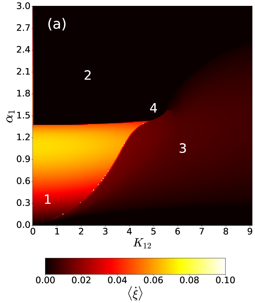
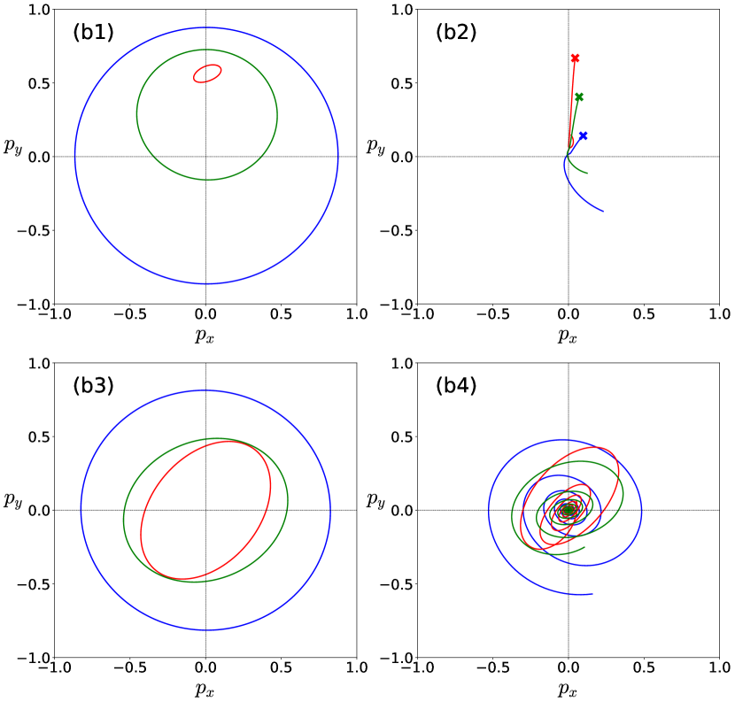
Figure 2: (a) Heatmap in $\alpha_{1}\times K_{12}$ parameter space showing the time averaged detuning $\langle\dot{\xi}\rangle$ obtained via numerical integration of Equations (25) to (28) with $\omega_{0}=0$ and $\Delta=1$. (b) Examples of $\vec{p}$ trajectories illustrating the different dynamics that occur on the system. The points that corresponds to each subpanel is indicated by numbers on (a). In all cases, blue lines refers to $\mathcal{G}_{1}$, red to $\mathcal{G}_{2}$ and green to $\mathcal{G}_{1}+\mathcal{G}_{2}$.

With the different outcomes of the combined motion elucidated, we can now analyze the effects of changing the parameters of the system. In particular, the effect of $J_{2}$, since for a fixed natural frequency distribution, the ratio between $K$ and $J$ dictates the dominating dynamic for a one module system. Thus, we performed numerical integrations of Equations (25) to (28) varying $J_{2}$. The heatmaps for the total order parameter $\langle p_{t}\rangle$ are shown in Figure 3. It can be seen that as $J_{2}$ increases the asynchronous region shrinks towards the bottom right boundaries for $J_{2}=5$ (Figure 3-(b)) until vanishing completely in Figure 3-(a)), which corresponds to $J_{2}=6$.

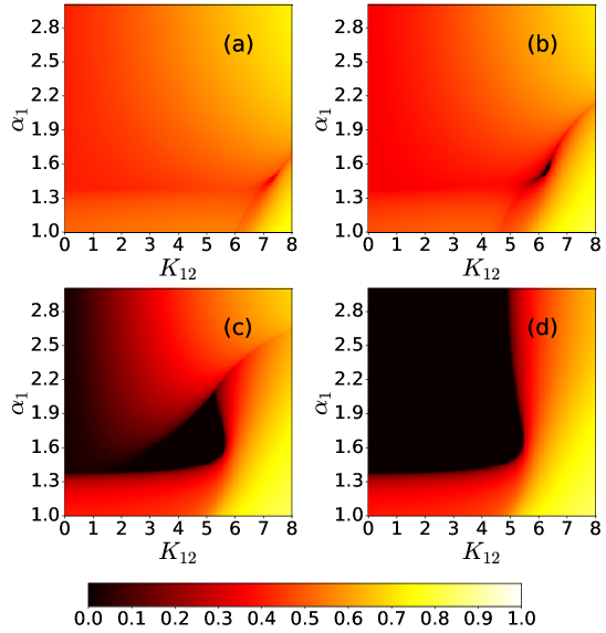
Figure 3: Heatmap in $\alpha_{1}\times K_{12}$ parameter space showing the time averaged order parameter $\langle p_{T}\rangle$, obtained via numerical integration of Equations (25) to (28) with $\omega_{0}=0$ and $\Delta=1$. $\mathbf{K}_{1}$ consist of $K_{1}=10$ and $\alpha$ variable while $\mathbf{K}_{2}$ consists in (a) $J_{2}=6$; (b) $J_{2}=5$; (c)$J_{2}=2$; (d)$J_{2}=0$.

The case of $J_{2}=0$, Figure 3-(d), is particularly interesting , as the dynamical equations become simple enough for analytical treatment. It corresponds to module $\mathcal{G}_{2}$ composed of free oscillators, driven only by their connections with $\mathcal{G}_{1}$. To calculate the asynchronous boundary we set $J_{2}=0$ in Equations (25) to (28) and combine equations for $\dot{\psi}_{1}$ and $\dot{\psi}_{2}$ into one for the phase difference $\dot{\xi}=\dot{\psi}_{1}-\dot{\psi}_{2}$ to obtain

$$\dot{p}_{1} =-\Delta p_{1}+\frac{p_{1}}{2}(1-p_{1}^{2})K_{1}\operatorname{cos}\alpha_{1}+\frac{p_{2}}{2}(1-p_{1}^{2})K_{12}\operatorname{cos}\xi,$$

$$\dot{p}_{2} =-\Delta p_{2}+\frac{p_{1}}{2}(1-p_{2}^{2})K_{12}\operatorname{cos}\xi,$$

$$\dot{\xi} =-\frac{1+p_{1}^{2}}{2}K_{1}\operatorname{sin}\alpha_{1}-\dfrac{K_{12}\sin{\xi}}{2}\left[\frac{p_{2}}{p_{1}}(1+p_{1}^{2})+\frac{p_{1}}{p_{2}}(1+p_{2}^{2})\right].$$

In equilibrium, when $p_{1}\to 0$ and $p_{2}\to 0$, we can approximate $(1-p_{1})\approx 1$ and $(1-p_{2})\approx 1$. Defining the auxiliary ratio $g=p_{2}/p_{1}$, the equations can be written as

$$-2g\Delta +gK_{1}\operatorname{cos}\alpha_{1}+K_{12}\operatorname{cos}\xi=0,$$ (29)

$$-2\Delta +gK_{12}\operatorname{cos}\xi=0,$$ (30)

$$-K_{1}\operatorname{sin}\alpha_{1} -K_{12}\sin{\xi}\left[g+\frac{1}{g}\right]=0.$$ (31)

Now, we can eliminate $g$ and $\cos\xi$ after some algebraic manipulation and write a single equation that involves variables $\cos\alpha_{1}$ and $K_{12}$ and parameters $K_{1}$ and $\Delta$:

$$4\Delta^{2}K^{2}_{1}-64\Delta^{3}K_{1}\cos{\alpha_{1}}+64\Delta^{4}-K_{12}^{2}(K_{1}\cos{\alpha_{1}}-4\Delta)^{2}-2\Delta K^{3}_{1}\cos{\alpha_{1}}+16\Delta^{2}K^{2}_{1}\cos^{2}{\alpha_{1}}=0.$$ (32)

Therefore, for a given set of parameters ($\Delta$;$K_{12}$;$K_{1}$), one can solve Equation (32) to find $\alpha_{1}$ that delimits the asynchronous region. A comparison between the boundary extracted directly from Figure 3-(d) and by solving Equation (32) can be found in Figure 4. It can be seen that the analytical curve in red delimits perfectly the hatched asynchronous region.

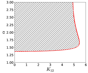
Figure 4: Comparison between the analytical dessincronization boundary (full red line) and the region obtained by direct integration of Equations (25) to (28) (hatched region) for $\omega_{0}=0$, $\Delta=1$ and $K_{1}=10$.

IV Simulations

Although the Ott-Antonsen ansatz enabled several analytical treatments and expanded the computational limit for numerical calculations [30, 12, 32, 33, 16] the constraint of Lorenz distribution of natural frequencies imposed by the ansatz restricts its range of applications. Therefore, to further support our analysis, we performed direct simulations with oscillators using Gaussian distributions of natural frequencies.

The first case is a scenario that mimics the system in the previous sections, a complete graph with $N=10000$ oscillators split into two groups with different coupling matrices. We made the same considerations as in the beginning of Section III, setting module $\mathcal{G}_{1}$ with $K_{1}=10$ and variable $\alpha_{1}$ while module $\mathcal{G}_{2}$ have $J_{2}=3$. By performing numerical integration of Equation (13) for each oscillator, we calculated the time averaged order parameter $\langle p\rangle$ and constructed the heatmaps in $\alpha_{1}\times K_{12}$ space, shown in Figure 5. The existence of an asynchronous region in approximate shape and position as in Figure 1 indicates that this behavior is somehow general and robust to other frequency distributions. In addition, the qualitative behaviors of $\langle p\rangle$ for each module and the system as a whole are similar to those found by the ansatz.

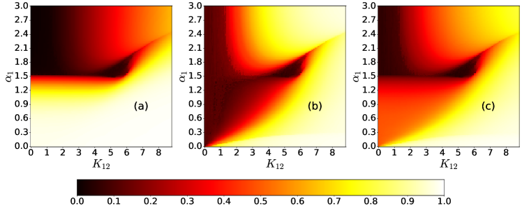
Figure 5: Time averaged order parameter $\langle p\rangle$ for a complete graph divided into two modules of $N=5000$ oscillators each with natural frequencies extracted from a Gaussian distribution with average $\omega_{0}=0$ and variance $\Delta=1$. (a) Module 1 ; (b) Module 2 and (c) Both modules.

Going one step closer to real systems, we relaxed the all-to-all interaction considered previously and performed simulations on synthetic modular networks. Those graphs were built using the random partition algorithm[34], in which we assign $N$ nodes to $\Omega$ partitions and try to connect every pair $(i,j)$ with probabilities $p_{in}$ or $p_{out}$ if nodes are within the same partition or not, respectively. For these simulations, we choose $N=1000$, two partitions and average degree $\langle k\rangle=10$. Therefore, the connection probabilites can be equated as

$$\dfrac{N(N-1)}{4}p_{in}+\dfrac{N^{2}}{4}p_{out}=\langle k\rangle.$$ (33)

We set $p_{in}=\lambda p_{out}$ and vary $\lambda$ in order to investigate the effects of connection density between modules in the equilibrium states. We set the same parameters: $K_{1}=10$, variable $\alpha_{1}$ and $J_{2}=3$ and performed the numerical integrations, calculating $\langle p\rangle$ and constructing the heatmaps shown in Figure 6. For $\lambda=3$, that corresponds to Figures 6-(a) to (c), the caracteristic asynchronous region presented in previous analysis can be seen clearly. It is important to notice that since the average number of connections between oscillators is small, the values of $K_{12}$ necessary to observe the different behaviors are much larger than in the all-to-all system. The shape of the heatmaps is qualitatively similar to the one obtained by the ansatz, aside from the emergence of a second asynchronous region for $\alpha_{1}$ close to 3. By increasing $\lambda$ to $5$, Figures 6-(d)-(f), the dilution of edges between modules drastically changes the heatmaps, with a much larger disordered region. Finally, in Figures 6-(g)-(i), in which $\lambda=10$, the heatmaps are similar of those with $\lambda=5$, with the asynchronous region dislocated to larger values of $K_{12}$. In addition, $\langle p\rangle$ becames independent of intramodule coupling for $K_{12}<10$. In this situation, the fraction of edges connecting oscillators from $\mathcal{G}_{1}$ to module $\mathcal{G}_{2}$ is so small that modules can be considered independent. We conjecture that for $\lambda$ large enough, no matter how large $K_{12}$ is, the mutual influence of the modules will be irrisory to change their dynamic.

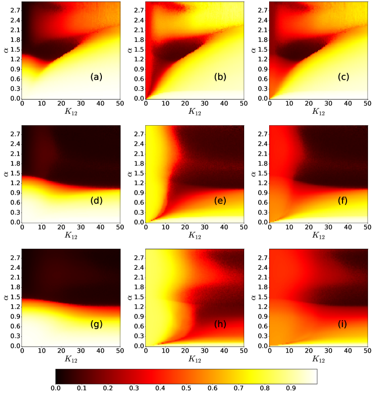
Figure 6: Time averaged order parameter $\langle p\rangle$ for a random partition graph divided into two modules summing $N=1000$ oscillators with natural frequencies extracted from a Gaussian distribution with average $\omega_{0}=0$ and variance $\Delta=1$. $\mathbf{K}_{1}$ consists of $K_{1}=10$ and variable $\alpha_{1}$ while $\mathbf{K}_{2}$ consists only on $J_{2}=3$. (a) $\mathcal{G}_{1}$ and $\lambda=3$ ; (b) $\mathcal{G}_{2}$ and $\lambda=3$ ; (c) $\mathcal{G}_{1}+\mathcal{G}_{2}$ and $\lambda=3$ ; (d) $\mathcal{G}_{1}$ and $\lambda=5$ ; (e) $\mathcal{G}_{2}$ and $\lambda=5$ ; (f) $\mathcal{G}_{1}+\mathcal{G}_{2}$ and $\lambda=5$ ; (g) $\mathcal{G}_{1}$ and $\lambda=10$ ; (h) $\mathcal{G}_{2}$ and $\lambda=10$ ; (i) $\mathcal{G}_{1}+\mathcal{G}_{2}$ and $\lambda=10$.

V Discussion and Conclusions

We investigated the dynamic of matrix coupled Kuramoto oscillators on a two module system with different matrices $\mathbf{K}$. By applying the Ott-Antonsen ansatz, we were able to reduce the problem to four differential equations describing the magnitude and phase of order parameter $p$ for each module. However, further analytical treatment was not possible due to the generalized frustration, induced by parameter $J$. Therefore, we selected a few particular and extreme cases to investigate in detail, performing numerical integration of the ansatz’s equations.

We set the parameters of the first module $\mathcal{G}_{1}$ to match Kuramoto-Sakaguchi oscillators ($K_{1}\neq 0$, $\alpha_{1}\neq 0$, $J_{1}=0$). Module $\mathcal{G}_{2}$, on the other hand, had complementary parameters ($K_{2}=0$, $\alpha_{2}=0$, $J_{2}\neq 0$), being in the phase tuned synchronization region, in which the phase of the oscillators synchronize in the direction of the principal eigenvector of the coupling matrix $\mathbf{K}$. For $K_{1}=10$ and $J_{2}=3$, we calculated the time averaged order parameter $\langle p\rangle$ and the time averaged detuning $\langle\dot{\xi}\rangle$, constructing heatmaps in $K_{12}\times\alpha$ plane. We identified four major regimes for the system’s dynamic: a region in which both modules behave independently, maintaining their uncoupled dynamic; a region where $\mathcal{G}_{1}$ dominates de dynamics, so that both modules rotate at similar frequency; a third region where $\mathcal{G}_{2}$ dominates and both modules tune their phases to a specific direction and; finally an asynchronous region. This last region is the most surprising one, indicating that interactions between different synchronized modules with same natural frequency and positive coupling may be somehow destructive. The size of the asynchronous boundary shrinks as $J$ increases, vanishing completely for $J_{2}=6$. For $J_{2}=0$ the equations became simple enough to allow analytical treatment and the boundary between disordered and collective motion was calculated.

In order to investigate the robustness of our findings, we also performed simulations for oscillators with Gaussian distribution of natural frequencies, in which the Ott-Antonsen ansatz is no longer applicable. For complete graphs, in which interactions between oscillators are all-to-all, the same dynamics as those obtained by the ansatz were found. For random modular graphs, in which the average number of links between oscillators is small, the qualitatively behavior was confirmed for sufficiently connected modules. However, if the modules are weakly connected, they always behave independently, no matter how strong the intermodular coupling is.

A natural prospect of this study is to consider systems with more modules and an ensemble of coupling matrices, that may lead to even more interesting and richer dynamics. In addition, the use of real modular graphs, such as neuronal networks, as substrates for matrix coupled oscillators may give new insights into the synchronization phenomena.

- [1] A. Winfree, The Geometry of Biological Time. Interdisciplinary Applied Mathematics, Springer New York, 2001.
- [2] S. Strogatz, Sync: The Emerging Science of Spontaneous Order. Hyperion Books, 2003.
- [3] C. M. Gray, “Synchronous oscillations in neuronal systems: mechanisms and functions,” J Comput Neurosci, vol. 1, pp. 11–38, June 1994.
- [4] J. Buck, “Synchronous rhythmic flashing of fireflies. ii.,” The Quarterly Review of Biology, vol. 63, no. 3, pp. 265–289, 1988. PMID: 3059390.
- [5] A. Moiseff and J. Copeland, “Firefly synchrony: a behavioral strategy to minimize visual clutter,” Science, vol. 329, p. 181, July 2010.
- [6] S. Boccaletti, A. Pisarchik, C. Genio, and A. Amann, Synchronization: From Coupled Systems to Complex Networks. Cambridge University Press, 2018.
- [7] E. Tognoli and J. Kelso, “The metastable brain,” Neuron, vol. 81, no. 1, pp. 35–48, 2014.
- [8] P. J. Uhlhaas and W. Singer, “Neural synchrony in brain disorders: Relevance for cognitive dysfunctions and pathophysiology,” Neuron, vol. 52, pp. 155–168, Oct. 2006.
- [9] Y. Kuramoto, “Self-entrainment of a population of coupled non-linear oscillators,” in International Symposium on Mathematical Problems in Theoretical Physics (H. Araki, ed.), (Berlin, Heidelberg), pp. 420–422, Springer Berlin Heidelberg, 1975.
- [10] J. Gómez-Gardeñes, S. Gómez, A. Arenas, and Y. Moreno, “Explosive synchronization transitions in scale-free networks,” Phys. Rev. Lett., vol. 106, p. 128701, Mar 2011.
- [11] F. A. Rodrigues, T. K. D. Peron, P. Ji, and J. Kurths, “The kuramoto model in complex networks,” Physics Reports, vol. 610, pp. 1–98, 2016. The Kuramoto model in complex networks.
- [12] L. M. Childs and S. H. Strogatz, “Stability diagram for the forced kuramoto model,” Chaos: An Interdisciplinary Journal of Nonlinear Science, vol. 18, no. 4, p. 043128, 2008.
- [13] C. A. Moreira and M. A. de Aguiar, “Global synchronization of partially forced kuramoto oscillators on networks,” Physica A: Statistical Mechanics and its Applications, vol. 514, pp. 487–496, 2019.
- [14] K. P. O’Keeffe, H. Hong, and S. H. Strogatz, “Oscillators that sync and swarm,” Nature Communications, vol. 8, Nov. 2017.
- [15] J. U. F. Lizárraga and M. A. M. de Aguiar, “Synchronization of sakaguchi swarmalators,” Phys. Rev. E, vol. 108, p. 024212, Aug 2023.
- [16] G. L. Buzanello, A. E. D. Barioni, and M. A. M. de Aguiar, “Matrix coupling and generalized frustration in kuramoto oscillators,” Chaos: An Interdisciplinary Journal of Nonlinear Science, vol. 32, no. 9, p. 093130, 2022.
- [17] R. Fariello and M. A. M. de Aguiar, “Exploring the phase diagrams of multidimensional Kuramoto models,” Chaos, Solitons & Fractals, vol. 179, p. 114431, Feb. 2024.
- [18] S. Chandra, M. Girvan, and E. Ott, “Continuous versus discontinuous transitions in the -dimensional generalized kuramoto model: Odd is different,” Phys. Rev. X, vol. 9, p. 011002, Jan 2019.
- [19] J. Zhu, “Synchronization of kuramoto model in a high-dimensional linear space,” Physics Letters A, vol. 377, no. 41, pp. 2939–2943, 2013.
- [20] H. Sakaguchi and Y. Kuramoto, “A Soluble Active Rotater Model Showing Phase Transitions via Mutual Entertainment,” Progress of Theoretical Physics, vol. 76, pp. 576–581, Sept. 1986.
- [21] M. A. M. de Aguiar, “Generalized frustration in the multidimensional Kuramoto model,” Physical Review E, vol. 107, p. 044205, Apr. 2023.
- [22] E. Oh, K. Rho, H. Hong, and B. Kahng, “Modular synchronization in complex networks,” Physical Review E, vol. 72, p. 047101, Oct. 2005.
- [23] K. Park, Y.-C. Lai, S. Gupte, and J.-W. Kim, “Synchronization in complex networks with a modular structure,” Chaos: An Interdisciplinary Journal of Nonlinear Science, vol. 16, p. 015105, Mar. 2006.
- [24] P. S. Skardal and J. G. Restrepo, “Hierarchical synchrony of phase oscillators in modular networks,” Physical Review E, vol. 85, p. 016208, Jan. 2012.
- [25] S. R. Ujjwal, N. Punetha, and R. Ramaswamy, “Phase oscillators in modular networks: The effect of nonlocal coupling,” Physical Review E, vol. 93, p. 012207, Jan. 2016.
- [26] A. Lancichinetti, S. Fortunato, and F. Radicchi, “Benchmark graphs for testing community detection algorithms,” Phys. Rev. E, vol. 78, p. 046110, Oct 2008.
- [27] M. Winding, B. D. Pedigo, C. L. Barnes, H. G. Patsolic, Y. Park, T. Kazimiers, A. Fushiki, I. V. Andrade, A. Khandelwal, J. Valdes-Aleman, F. Li, N. Randel, E. Barsotti, A. Correia, R. D. Fetter, V. Hartenstein, C. E. Priebe, J. T. Vogelstein, A. Cardona, and M. Zlatic, “The connectome of an insect brain,” Science, vol. 379, no. 6636, p. eadd9330, 2023.
- [28] L. M. Sanchez-Rodriguez, Y. Iturria-Medina, P. Mouches, and R. C. Sotero, “Detecting brain network communities: Considering the role of information flow and its different temporal scales,” NeuroImage, vol. 225, p. 117431, 2021.
- [29] M. A. Porter, J. Onnela, and P. J. Mucha, “Communities in networks.”.
- [30] E. Ott and T. M. Antonsen, “Low dimensional behavior of large systems of globally coupled oscillators,” Chaos: An Interdisciplinary Journal of Nonlinear Science, vol. 18, p. 037113, 09 2008.
- [31] T. Tanaka, “Solvable model of the collective motion of heterogeneous particles interacting on a sphere,” New Journal of Physics, vol. 16, p. 023016, Feb. 2014.
- [32] P. S. Skardal and A. Arenas, “Higher order interactions in complex networks of phase oscillators promote abrupt synchronization switching,” Communications Physics, vol. 3, pp. 1–6, Nov. 2020.
- [33] A. E. D. Barioni and M. A. M. de Aguiar, “Complexity reduction in the 3D Kuramoto model,” Chaos, Solitons & Fractals, vol. 149, p. 111090, Aug. 2021.
- [34] U. Brandes, M. Gaertler, and D. Wagner, “Experiments on graph clustering algorithms,” in Algorithms - ESA 2003 (G. Di Battista and U. Zwick, eds.), (Berlin, Heidelberg), pp. 568–579, Springer Berlin Heidelberg, 2003.