Streamlining in the Riemannian Realm:
Efficient Riemannian Optimization with Loopless Variance Reduction

Abstract

In this study, we investigate stochastic optimization on Riemannian manifolds, focusing on the crucial variance reduction mechanism used in both Euclidean and Riemannian settings. Riemannian variance-reduced methods usually involve a double-loop structure, computing a full gradient at the start of each loop. Determining the optimal inner loop length is challenging in practice, as it depends on strong convexity or smoothness constants, which are often unknown or hard to estimate. Motivated by Euclidean methods, we introduce the Riemannian Loopless SVRG (R-LSVRG) and PAGE (R-PAGE) methods. These methods replace the outer loop with probabilistic gradient computation triggered by a coin flip in each iteration, ensuring simpler proofs, efficient hyperparameter selection, and sharp convergence guarantees. Using R-PAGE as a framework for non-convex Riemannian optimization, we demonstrate its applicability to various important settings. For example, we derive Riemannian MARINA (R-MARINA) for distributed settings with communication compression, providing the best theoretical communication complexity guarantees for non-convex distributed optimization over Riemannian manifolds. Experimental results support our theoretical findings.

1 Introduction

In this work we study finite-sum optimization problem:

$$\min_{x\in\mathcal{X}\subset\mathcal{M}}\ f(x)\ \triangleq\ \frac{1}{n}\sum_{i=1}^{n}f_{i}(x),$$ (1)

where $(\mathcal{M},\mathfrak{g})$ represents a Riemannian manifold equipped with the Riemannian metric $\mathfrak{g}$, and $\mathcal{X}\subset\mathcal{M}$ is a geodesically convex set. Additionally, we assume that each function $f_{i}:\mathcal{M}\to\mathbb{R}$ is geodesically $L$-smooth.

This formulation demonstrates its applicability across a wide range of practical scenarios, encompassing fundamental tasks such as principal component analysis (PCA) (Wold et al., 1987) and independent component analysis (ICA) (Lee and Lee, 1998). Additionally, it extends its utility to address challenges like the completion and recovery of low-rank matrices and tensors (Tan et al., 2014; Vandereycken, 2013; Mishra and Sepulchre, 2014; Kasai and Mishra, 2016), dictionary learning (Cherian and Sra, 2016; Sun et al., 2016), optimization under orthogonality constraints (Edelman et al., 1998; Moakher, 2002), covariance estimation (Wiesel, 2012), learning elliptical distributions (Sra and Hosseini, 2013), and Poincaré embeddings (Nickel and Kiela, 2017). Furthermore, it proves effective in handling Gaussian mixture models (Hosseini and Sra, 2015) and low-rank multivariate regression (Meyer et al., 2011). This versatility makes it a valuable tool for tackling numerous problems in various settings.

In addressing problems involving manifold constraints, a traditional approach involves alternating between optimization in the ambient Euclidean space and the process of "projecting" onto the manifold (Hauswirth et al., 2016). The most popular method in this class is projected stochastic gradient descent (Luenberger, 1972; Calamai and Moré, 1987). Furthermore, this concept is employed by other well-established methods. For example, two widely recognized techniques used to compute the leading eigenvector of symmetric matrices—power iteration (Bai et al., 1996) and Oja’s algorithm (Oja, 1992)—are based on a projecting approach. However, these methods tend to suffer from high computational costs, when projecting onto certain manifolds (e.g., positive-definite matrices), which could be expensive in large-scale learning problems Zhang et al. (2016); Zhou et al. (2019).

An alternative option is to utilize Riemannian optimization, a method that directly interacts with the specific manifold under consideration (da Cruz Neto et al., 1998). This approach enables Riemannian optimization to interpret the constrained optimization problem (1) as an unconstrained problem on a manifold, eliminating the need for projections (Bonnabel, 2013; Zhang and Sra, 2016). What’s particularly significant is the conceptual perspective: by formulating the problem within a Riemannian framework, one can gain insights into the geometry of the problem (Zhang and Sra, 2018). This not only facilitates more precise mathematical analysis but also leads to the development of more efficient optimization algorithms.

The expression of equation (1) in Euclidean form, where $\mathcal{M}=\mathbb{R}^{d}$ and $\mathfrak{g}$ represents the Euclidean inner product, has been a central focus of substantial algorithmic advancements in the fields of machine learning and optimization (Bertsekas and Tsitsiklis, 2000; Goodfellow et al., 2016; Sun, 2020; Ajalloeian and Stich, 2020; Demidovich et al., 2023). This evolution traces back to the foundational work of Stochastic Gradient Method (SGD) by Robbins and Monro (1951). However, both batch and stochastic gradient methods grapple with considerable computational demands. When addressing finite sum problems with $n$ components, the full-gradient method requires $n$ derivatives at each step, while the stochastic method requires only one derivative (Bottou et al., 2018). Nevertheless, Stochastic Gradient Descent suffers from a slow sublinear rate (Gower et al., 2019; Khaled and Richtárik, 2023; Paquette et al., 2021). Tackling these challenges has spurred notable advancements in faster stochastic optimization within vector spaces, leveraging variance reduction techniques (Schmidt et al., 2017; Johnson and Zhang, 2013; Defazio et al., 2014; Konečný and Richtárik, 2017).

In conjunction with numerous recent studies (Song et al., 2020; Gower et al., 2020; Dragomir et al., 2021), these algorithms showcase accelerated convergence compared to the original gradient descent algorithms across various scenarios, including strongly convex (Gorbunov et al., 2020), general convex (Khaled et al., 2023), and non-convex settings (Reddi et al., 2016; Allen-Zhu and Hazan, 2016; Fang et al., 2018). In order to simplify complicated structures of variance-reduced methods, loopless versions were proposed initially in strongly convex settings (Hofmann et al., 2015; Kovalev et al., 2020). Later, this approach was adopted in non-convex and general convex settings (Li et al., 2021; Horváth et al., 2022; Khaled et al., 2023). The loopless structure allows us to obtain practical parameters and make proofs more elegant.

In the context of distributed learning, where each individual function in equation (1) is stored on a separate device, the communication compression approach is frequently utilized to ease communication load (Alistarh et al., 2017). The initial concept involved employing quantization or sparsification of gradients, sending compressed gradients to the server for aggregation, and subsequently performing a step (Wangni et al., 2018). However, owing to the high variance or errors linked with compression operators, a direct application does not consistently ensure improved convergence (Alistarh et al., 2018; Shi et al., 2019). To tackle this issue, akin to the SGD scenario, various mechanisms for variance reduction (Mishchenko et al., 2019; Horváth et al., 2023) and error compensation in compression (Stich et al., 2018; Stich and Karimireddy, 2019; Richtárik et al., 2021) have been proposed. The current state-of-the-art method in non-convex scenario is MARINA (Gorbunov et al., 2021), which allows to obtain optimal $\mathcal{O}\left(\frac{1+\omega/\sqrt{n}}{\varepsilon^{2}}\right)$ communication complexity.

In recent times, there has been a growing interest in exploring the Riemannian counterparts of batch and stochastic optimization algorithms. The pioneering work by Zhang and Sra (2016) marked the first comprehensive analysis of the global complexity of batch and stochastic gradient methods for geodesically convex functions. Subsequent research by Zhang et al. (2016); Kasai et al. (2016); Sato et al. (2019); Han and Gao (2021) focused on improving the convergence rate for finite-sum problems through the application of variance reduction techniques. Additionally, there has been an analysis of the near-optimal variance reduction method for non-convex Riemannian optimization problems, known as R-SPIDER (Zhang et al., 2018; Zhou et al., 2019). While this method boasts strong theoretical guarantees, its practical implementation poses challenges due to its double-loop structure. Determining practical parameters is particularly difficult, as the length of the inner loop often depends on condition number or smoothness constant and the desired level of accuracy, denoted by $\varepsilon$.

2 Contributions

Below, we outline the primary contributions of this paper.

• We introduce R-LSVRG, a Riemannian Loopless Stochastic Variance Reduced Gradient Descent method inspired by the Euclidean L-SVRG method (Kovalev et al., 2020). In its loopless form, we eliminate the inner loop and replace it with a biased coin-flip mechanism executed at each step of the method. This coin-flip determines when to compute the gradient by making a pass over the data. Alternatively, this approach can be interpreted as incorporating an inner loop of random length. The resulting method is easier to articulate, understand, and analyze. We demonstrate that R-LSVRG exhibits the same rapid theoretical convergence rate of $\mathcal{O}\left(\left(n+\frac{L^{2}\zeta}{\mu^{2}}\right)\log\frac{1}{\varepsilon}\right)$ as its looped counterpart (Zhang et al., 2016). Moreover, our analysis allows the expected length of the inner loop to be $\mathcal{O}(n)$, independent of the strong convexity constant $\mu$ and the smoothness constant $L$, making the method more practically applicable.

• We present R-PAGE, a Riemannian adaptation of the Probabilistic Gradient Estimator designed for non-convex optimization, drawing inspiration from the research conducted by Li et al. (2021). We analyze R-PAGE for optimizing geodesically smooth stochastic non-convex functions. Our analysis shows that this method achieves the best-known rates of $\mathcal{O}\left(n+\frac{n^{1/2}}{\varepsilon^{2}}\right)$ in the finite sum setting and $\mathcal{O}\left(\frac{1}{\varepsilon^{3}}\right)$ in the online setting. Moreover, these guarantees align with the lower bound established by (Fang et al., 2018) in the Euclidean case. Similar to the R-LSVRG method, the R-PAGE algorithm also employs a coin-flip approach, making the length of the inner loop random. Our analysis allows us to choose the expected length to be $\mathcal{O}(n)$, independent of the smoothness constant $L$ and the accuracy $\varepsilon$, rendering the method practical.

• Employing R-PAGE as a foundation for non-convex Riemannian optimization, we showcase its adaptability across diverse and significant contexts. As an illustration, we formulate Riemannian MARINA (R-MARINA), specifically tailored for distributed scenarios incorporating communication compression and variance reduction. This development not only extends the utility of R-PAGE but also establishes, to the best of our knowledge, the best theoretical communication complexity assurances for non-convex distributed optimization over Riemannian manifolds, aligning with the lower bounds in the Euclidean case (Gorbunov et al., 2021).

3 Preliminaries

A Riemannian manifold $(\mathcal{M},\mathfrak{g})$ is a real smooth manifold $\mathcal{M}$ equipped with a Riemannian metric $\mathfrak{g}$. This metric induces an inner product structure in each tangent space $T_{x}\mathcal{M}$ associated with every $x\in\mathcal{M}$. The inner product of vectors $u$ and $v$ in $T_{x}\mathcal{M}$ is denoted as $\langle u,v\rangle\triangleq\mathfrak{g}_{x}(u,v)$, and the norm of a vector $u\in T_{x}\mathcal{M}$ is defined as $\|u\|\triangleq\sqrt{\mathfrak{g}_{x}(u,u)}$. The angle between vectors $u$ and $v$ is given by $\arccos\frac{\langle u,v\rangle}{\|u\|\|v\|}$.

A geodesic is a curve parameterized by constant speed $\gamma:[0,1]\to\mathcal{M}$ that locally minimizes distance. The exponential map $\mathrm{Exp}_{x}:T_{x}\mathcal{M}\to\mathcal{M}$ maps a vector $v$ in $T_{x}\mathcal{M}$ to a point $y$ on $\mathcal{M}$ such that there exists a geodesic $\gamma$ with $\gamma(0)=x$, $\gamma(1)=y$, and $\dot{\gamma}(0)\triangleq\frac{d}{dt}\gamma(0)=v$.

If there is a unique geodesic between any two points in $\mathcal{X}\subset\mathcal{M}$, the exponential map has an inverse $\mathrm{Exp}_{x}^{-1}:\mathcal{X}\to T_{x}\mathcal{M}$. The geodesic is the uniquely shortest path with $\|\mathrm{Exp}_{x}^{-1}(y)\|=\|\mathrm{Exp}_{y}^{-1}(x)\|$, defining the geodesic distance between $x$ and $y\in\mathcal{X}$.

Parallel transport, denoted as $\Gamma_{x}^{y}:T_{x}\mathcal{M}\to T_{y}\mathcal{M}$, is a mapping that transports a vector $v\in T_{x}\mathcal{M}$ to $\Gamma_{x}^{y}v\in T_{y}\mathcal{M}$. This process retains both the norm and, in a figurative sense, the "direction," akin to translation in $\mathbb{R}^{d}$. Notably, a tangent vector of a geodesic $\gamma$ maintains its tangential orientation when parallel transported along $\gamma$. Moreover, parallel transport preserves inner products.

In our work, we will employ various crucial definitions and standard assumptions for theoretical analysis.

Definition 1 (Riemannian gradient).

The Riemannian gradient, denoted as $\nabla f(x)$, represents a vector in the tangent space $T_{x}(\mathcal{M})$ such that $\frac{d(f(\gamma(t)))}{dt}|_{t=0}=\langle v,\nabla f(x)\rangle_{x},$ holds true for any $v\in T_{x}\mathcal{M}.$

Assumption 1 (Geodesic convexity).

A function $f:\mathcal{X}\to\mathbb{R}$ is considered geodesically convex if, for any $x$ and $y$ in $\mathcal{X}$, and for any geodesic $\gamma$ connecting $x$ to $y$ such that $\gamma(0)=x$ and $\gamma(1)=y$, the inequality

$$f(\gamma(t))\leq(1-t)f(x)+tf(y)$$

holds for all $t$ in the interval $[0,1].$

Demonstrably, an equivalent definition asserts that, for any $x$ and $y$ in $\mathcal{X}$,

$$f(y)\geq f(x)+\langle g_{x},\mathrm{Exp}_{x}^{-1}(y)\rangle_{x},$$

where $g_{x}$ serves as a subgradient of $f$ at $x$, or the gradient in case $f$ is differentiable. Here, $\langle\cdot,\cdot\rangle_{x}$ signifies the inner product within the tangent space at $x$ induced by the Riemannian metric.

Assumption 2 (Geodesic strong convexity).

A function $f:\mathcal{X}\to\mathbb{R}$ is considered geodesically $\mu$-strongly convex ($\mu$-strongly g-convex) if, for any $x$ and $y$ in $\mathcal{X}$ and a subgradient $g_{x}$, the inequality holds:

$$f(y)\geq f(x)+\langle g_{x},\mathrm{Exp}_{x}^{-1}(y)\rangle_{x}+\frac{\mu}{2}d^{2}(x,y).$$

Assumption 3 (Geodesic smoothness).

A differentiable function $f:\mathcal{X}\to\mathbb{R}$ is considered geodesically $L$-smooth ($L$-g-smooth) if its gradient is geodesically $L$-Lipschitz ($L$-g-Lipschitz). This is expressed as, for any $x$ and $y$ in $\mathcal{X}$,

$$\|g_{x}-\Gamma_{y}^{x}g_{y}\|\leq L\|\mathrm{Exp}_{x}^{-1}(y)\|,$$

where $\Gamma_{y}^{x}$ represents the parallel transport from $y$ to $x$. In such cases, the following inequality holds:

$$f(y)\leq f(x)+\langle g_{x},\mathrm{Exp}^{-1}_{x}(y)\rangle+\frac{L}{2}\left\|\mathrm{Exp}^{-1}_{x}(y)\right\|^{2}.$$

Throughout the remainder of the paper, we will omit the index of the tangent space when its context is apparent.

Assumption 4 (Polyak-Łojasiewicz condition).

We assert that $f:\mathcal{M}\to\mathbb{R}$ satisfies the Polyak-Łojasiewicz condition (PŁ-condition) if $f^{*}$ uniformly bounds $f(x)$ from below for all $x\in\mathcal{M}$, and there exists $\mu>0$ such that

$$2\mu\left(f(x)-f^{*}\right)\leq\left\|f(x)\right\|^{2},\quad\forall;x\in\mathcal{X}.$$

Assumption 5 (Uniform lower bound).

There exists $f^{*}\in$ $\mathbb{R}$ such that $f(x)\geq f^{*}$ for all $x\in\mathbb{R}^{d}$.

We revisit an essential trigonometric distance bound, which holds significance for our analytical considerations.

Lemma 1 ((Zhang and Sra, 2016) Lemma 6).

If $a$, $b$, and $c$ represent the sides (i.e., side lengths) of a geodesic triangle in an Alexandrov space with curvature lower bounded by $\kappa_{\min}$, and $A$ denotes the angle between sides $b$ and $c$, then the following distance bound holds:

$$a^{2}\leq\frac{\sqrt{|\kappa_{\min}|}c}{\tanh(\sqrt{|\kappa_{\min}|}c)}b^{2}+c^{2}-2bc\cos(A).$$ (2)

In the subsequent sections, we adopt the notation $\zeta(\kappa_{\min},c)\stackrel{{\scriptstyle\text{def}}}{{=}}\frac{\sqrt{|\kappa_{\min}|}c}{\tanh(\sqrt{|\kappa_{\min}|}c)}$ for the curvature-dependent quantity defined in inequality (2). Leveraging Lemma 1, we can readily establish the following corollary. This corollary unveils a significant relationship between two consecutive updates within an iterative optimization algorithm on a Riemannian manifold with curvature bounded from below.

Corollary 1.

For any Riemannian manifold $\mathcal{M}$ where the sectional curvature is lower bounded by $\kappa_{\min}$ and for any point $x$, $x_{s}\in\mathcal{M}$, the update $x_{s+1}=\mathrm{Exp}_{x_{s}}(-\eta_{s}g_{x_{s}})$ adheres to the inequality:

$$\langle-g_{x_{s}},\mathrm{Exp}_{x_{s}}^{-1}(x)\rangle \leq\frac{1}{2\eta_{s}}\left(d^{2}(x_{s},x)-d^{2}(x_{s+1},x)\right)+\frac{\zeta(\kappa_{\min},d(x_{s},x))\eta_{s}}{2}\|g_{x_{s}}\|^{2}.$$

In our analysis, we employ an additional set of assumptions essential for handling the geometry of Riemannian manifolds. It is worth noting that the majority of practical manifold optimization problems can meet these assumptions.

Assumption 6.

We assume that

1. $f$ attains its optimum at $x^{*}\in\mathcal{X}$;

2. $\mathcal{X}$ is compact, and the diameter of $\mathcal{X}$ is bounded by $D$, that is, $\max_{x,y\in\mathcal{X}}d(x,y)\leq D$;

3. the sectional curvature in $\mathcal{X}$ is upper bounded by $\kappa_{\max}$, and within $\mathcal{X}$ the exponential map is invertible;

4. the sectional curvature in $\mathcal{X}$ is lower bounded by $\kappa_{\min}$.

We introduce a fundamental geometric constant with the objective of encapsulating and characterizing the impact and importance associated with the curvature of the manifold.

Definition 2 (Curvature-driven manifold term).

The term "curvature-driven manifold" refers to the constant described below:

$$\zeta=\left\{\begin{array}[]{ll}\frac{\sqrt{|\kappa_{\min}|}D}{\tanh(\sqrt{|\kappa_{\min}|}D)},&\text{if }\kappa_{\min}<0,\\ 1,&\text{if }\kappa_{\min}\geq 0.\end{array}\right.$$

4 Riemannian LSVRG

Algorithm 1 Riemannian Loopless Stochastic Variance Reduced Gradient Descent (R-LSVRG)

1:Parameters: initial point $x^{0}\in\mathcal{M},$ $y^{0}=x^{0},$ learning rate $\eta>0$

2:for $k=0,1,2,\ldots$ do

3:     Sample $i\in[n]$ uniformly at random

4:     $g^{k}=\nabla f_{i}(x^{k})-\Gamma_{y^{k}}^{x^{k}}\left(\nabla f_{i}(y^{k})-\nabla f(y^{k})\right)$

5:     $x^{k+1}=\mathrm{Exp}_{x^{k}}\left(-\eta g^{k}\right)$

6:     $y^{k+1}=\begin{cases}x^{k},&\text{with probability }p\\ y^{k},&\text{otherwise.}\end{cases}$

7:end for

In this section, we analyze the convergence guarantees of R-LSVRG for solving the problem (1), where each $f_{i}$ ($i\in[n]$) is g-smooth and $f$ is strongly g-convex. In this context, we show that R-LSVRG exhibits a linear convergence rate.

Algorithm 2 Riemannian ProbAbilistic Gradient Estimator (R-PAGE)

1:Parameters: $\text{ initial point }x^{0}\text{, stepsize }\eta>0\text{, minibatch size }B,b<B\text{, probability }p\in(0,1]$

2: $g^{0}=\nabla f_{B}(x^{0})$,   where $\nabla f_{B}$ is minibatch stochastic gradient estimator with size $B$

3:for $k=0,1,2,\ldots$ do

4:     $x^{k+1}=\mathrm{Exp}_{x^{k}}\left(-\eta g^{k}\right)$

5:      $g^{k+1}=\begin{cases}\nabla f_{B}(x^{k+1}),&\text{with probability }p\\ \Gamma_{x^{k}}^{x^{k+1}}\left(g^{k}\right)+\nabla f_{b}(x^{k+1})-\Gamma_{x^{k}}^{x^{k+1}}\left(\nabla f_{b}(x^{k})\right),&\text{otherwise.}\end{cases}$

6:end for

Theorem 1.

Assuming that in (1), each $f_{i}$ is differentiable and $L$-g-smooth on $\mathcal{X}$ (Assumption 3 holds), and $f$ is $\mu$-strongly g-convex on $\mathcal{X}$ (Assumption 2 holds). Additionally, let Assumption 6 hold. Choose the stepsize $0<\eta\leq\frac{\mu}{16L^{2}\zeta}.$ Then, the iterates of the Riemannian L-SVRG method (Algorithm 1) satisfy

$$\mathbb{E}\left[\Phi^{k}\right]\leq\left(\max\left\{1-\eta\mu,1-\frac{p}{2}\right\}\right)^{k}\Phi^{0},$$ (3)

where $\Phi^{k}\stackrel{{\scriptstyle\text{def}}}{{=}}d^{2}\left(x^{k},x^{*}\right)+\frac{3\mu^{2}}{64pL^{2}\zeta}\mathcal{D}^{k}$ and $\mathcal{D}^{k}\stackrel{{\scriptstyle\text{def}}}{{=}}\left\|\mathrm{Exp}^{-1}_{y^{k}}(x^{*})\right\|^{2}.$

Corollary 2.

With the assumptions outlined in Theorem 1, if we set $\eta=\frac{\mu}{16L^{2}\zeta}$, in order to obtain $\mathbb{E}[\Phi^{k}]\leq\varepsilon\Phi^{0}$, we find that the iteration complexity of Riemannian L-SVRG method (Algorithm 1) is given by

$$K=\mathcal{O}\left(\left(\frac{1}{p}+\frac{L^{2}\zeta}{\mu^{2}}\right)\log\frac{1}{\varepsilon}\right).$$

By examining equation (3), it becomes apparent that the contraction of the Lyapunov function is determined by $\max\{1-\eta\mu,1-\frac{p}{2}\}$. Due to the constraint $\eta\leq\frac{\mu}{16L^{2}\zeta}$, the first term is bounded from below by $1-\frac{\mu^{2}}{16L^{2}\zeta}$. Consequently, the complexity cannot surpass $\mathcal{O}\left(\frac{\zeta L^{2}}{\mu^{2}}\log\frac{1}{\varepsilon}\right)$. Regarding the total complexity, which is measured by the number of stochastic gradient calls, R-LSVRG, on average, invokes the stochastic gradient oracle $2+p(n-1)$ times in each iteration. Combining these two complexities yields a total complexity of $\mathcal{O}\left(\left(\frac{1}{p}+n+\frac{\zeta L^{2}}{\mu^{2}}+\frac{pn\zeta L^{2}}{\mu^{2}}\right)\log\frac{1}{\varepsilon}\right)$. It is noteworthy that choosing any $p\in\left[\min\{\frac{c}{n},\frac{c\mu^{2}}{L^{2}\zeta}\},\max\{\frac{c}{n},\frac{c\mu^{2}}{L^{2}\zeta}\}\right],$ where $c=\Theta(1)$, results in the optimal total complexity $\mathcal{O}\left(\left(n+\frac{L^{2}\zeta}{\mu^{2}}\right)\log\frac{1}{\varepsilon}\right)$. This resolution addresses a gap in R-SVRG theory, where the length of the inner loop (in our case, $\frac{1}{p}$ on average) must be proportional to $\mathcal{O}\left(\zeta L^{2}/\mu^{2}\right).$ Moreover, the analysis for R-LSVRG is more straightforward and offers deeper insights.

Let us succinctly formalize the aforementioned findings in the context of a corollary.

Corollary 3.

With the assumptions outlined in Theorem 1, if we set $\eta=\frac{\mu}{16L^{2}\zeta}$ and $p=\frac{1}{n}$, in order to obtain $\mathbb{E}[\Phi^{k}]\leq\varepsilon\Phi^{0}$, we find that the total computational complexity of Riemannian L-SVRG method (Algorithm 1) is given by

$$K=\mathcal{O}\left(\left(n+\frac{L^{2}\zeta}{\mu^{2}}\right)\log\frac{1}{\varepsilon}\right).$$

5 Riemannian PAGE

5.1 The Riemannian PAGE gradient estimator

The specific gradient estimator $g^{t+1}$ is formally defined in Line 5 of Algorithm 2. It is essential to note that the method employs the simple stochastic gradient with a large minibatch size (resembling a full batch in a finite sum setting) with a small probability $p$, and with a substantial probability $1-p$, it utilizes the previous gradient $g^{t}$ with a minor adjustment involving the difference of stochastic gradients computed at two points, namely, $x^{t}$ and $x^{t+1}$ (a measure aimed at reducing computational costs, especially considering that $b\ll B$).

In particular, when $p\equiv 1$, this aligns with vanilla minibatch Riemannian Stochastic Gradient Descent (R-SGD), and further, when the minibatch size is set to $B=n$, it simplifies to Riemannian Gradient Descent (R-GD). We present a straightforward formula for the optimal determination of $p$, expressed as $p\equiv\frac{b}{B+b}$. This formula proves sufficient for PAGE to achieve optimal convergence rates, with additional nuances elucidated in the convergence results.

5.2 Convergence in Non-Convex Finite-Sum Setting

In this section, we delve into an analysis of the convergence guarantees offered by R-PAGE in solving the problem (1), where each function $f_{i}$ (with $i\in[n]$) is characterized as g-smooth, and the function $f$ has a lower bound. Within this framework, we substantiate that R-PAGE demonstrates a convergence rate aligning with current state-of-the-art results.

Theorem 2.

Assuming that each $f_{i}$ in (1) is differentiable and $L$-g-smooth on $\mathcal{M}$ (Assumption 3 holds) and that $f$ is lower bounded on $\mathcal{M}$ (Assumption 5 holds), let $\delta^{0}\stackrel{{\scriptstyle\text{def}}}{{=}}f(x^{0})-f^{*}$. Select the stepsize $\eta$ such that $0<\eta\leq\frac{1}{L\left(1+\sqrt{\frac{1-p}{pb}}\right)},$ and the minibatch size $B=n,$ and the secondary minibatch size $b<B.$ Then, the iterates of the R-PAGE method (Algorithm 2) satisfy

$$\mathbb{E}\left[\left\|\nabla f(\widehat{x}^{K})\right\|^{2}\right]\leq\frac{2\delta^{0}}{\eta K},$$

where $\widehat{x}^{k}$ is chosen randomly from $x^{0},\ldots,x^{K-1}$ with uniform probability distribution.

Corollary 4.

With the assumptions outlined in Theorem 2, if we set $\eta=\frac{1}{L\left(1+\sqrt{\frac{1-p}{pb}}\right)}$, in order to obtain $\mathbb{E}\left[\left\|\nabla f\left(\widehat{x}^{K}\right)\right\|\right]\leq\varepsilon$, we find that the iteration complexity of R-PAGE method (Algorithm 2) is given by

$$K=\mathcal{O}\left(\left(1+\sqrt{\frac{1-p}{pb}}\right)\frac{L\delta^{0}}{\varepsilon^{2}}\right).$$

Additionally, in accordance with R-PAGE gradient estimator (refer to Line 5 of Algorithm 2), it is evident that, on average, it employs $pB+(1-p)b$ stochastic gradients for each iteration. Consequently, the computational load for stochastic gradient computations, denoted as $\#\operatorname{grad}$ (i.e., gradient complexity), can be expressed as: $\#\operatorname{grad}=B+K\left(pB+(1-p)b\right)=\mathcal{O}\left(B+\frac{2\delta_{0}L}{\varepsilon^{2}}\left(1+\sqrt{\frac{1-p}{pb}}\right)\left(pB+(1-p)b\right)\right).$

It is important to highlight that the initial $B$ in $\#\operatorname{grad}$ accounts for the computation of $g^{0}$ (refer to Line 2 in Algorithm 2). Subsequently, we present a parameter configuration that yields the best known convergence rate for the non-convex finite-sum problem (1).

Corollary 5.

With the assumptions outlined in Theorem 2, if we set $\eta=\frac{1}{L\left(1+\sqrt{\frac{1-p}{pb}}\right)}$, minibatch size $B=n$, secondary minibatch size $b\leq\sqrt{B}$ and $p\equiv\frac{b}{B+b}$, in order to obtain $\mathbb{E}\left[\left\|\nabla f\left(\widehat{x}^{K}\right)\right\|\right]\leq\varepsilon$, we find that the total computational complexity of Riemannian PAGE method (Algorithm 2) is given by

$$\#\operatorname{grad}=\mathcal{O}\left(n+\frac{\sqrt{n}}{\varepsilon^{2}}\right).$$

In the subsequent discussion, we delve into an analysis within a non-convex finite-sum setting under the Polyak-Łojasiewicz condition. This assumption allows us to assert a linear convergence rate.

Theorem 3.

Assuming that each $f_{i}$ in (1) is differentiable and $L$-g-smooth on $\mathcal{M}$ (Assumption 3 holds), also that $f$ is lower bounded on $\mathcal{M}$ (Assumption 5 holds) and it satisfies Polyak-Łojasiewicz condition (Assumption 4 holds) with constant $\mu$, let $\delta^{0}\stackrel{{\scriptstyle\text{def}}}{{=}}f(x^{0})-f^{*}$. Select the stepsize $\eta$ such that $\eta\leq\min\left\{\frac{1}{L\left(1+\sqrt{\frac{1-p}{pb}}\right)},\frac{p}{2\mu}\right\}.$ Then, the iterates of the Riemannian PAGE method (Algorithm 2) satisfy

$$\mathbb{E}\left[\Phi^{K}\right]\leq(1-\mu\eta)^{K}\delta^{0},$$

where $\Phi^{k}\stackrel{{\scriptstyle\text{def}}}{{=}}f\left(x^{k}\right)-f^{*}+\frac{2}{p}\left\|g^{k}-\nabla f\left(x^{k}\right)\right\|^{2}$ and $\Phi^{0}=\delta^{0}$, since $g^{0}=\nabla f(x^{0}).$

Corollary 6.

With the assumptions outlined in Theorem 3, if we set $\eta=\min\left\{\frac{1}{L\left(1+\sqrt{\frac{1-p}{pb}}\right)},\frac{p}{2\mu}\right\}$, in order to obtain $\mathbb{E}[\Phi^{k}]\leq\varepsilon\Phi^{0}$, we find that the iteration complexity of Riemannian R-PAGE method (Algorithm 2) is given by

$$K=\mathcal{O}\left(\left(\left(1+\sqrt{\frac{1-p}{pb}}\right)\frac{L}{\mu}+\frac{1}{p}\right)\log\frac{1}{\varepsilon}\right).$$

Similarly to general non-convex setting we can estimate the computational load for stochastic gradient computations: $\#\operatorname{grad}=B+K\left(pB+(1-p)b\right)=\mathcal{O}\left(B+\frac{2\delta_{0}L}{\varepsilon^{2}}\left(1+\sqrt{\frac{1-p}{pb}}\right)\left(pB+(1-p)b\right)\right).$ Following that, we introduce a parameter setup that produces the most favorable known convergence rate for the Riemannian non-convex finite-sum problem (1).

Corollary 7.

With the assumptions outlined in Theorem 3, if we set $\eta=\min\left\{\frac{1}{L\left(1+\sqrt{\frac{1-p}{pb}}\right)},\frac{p}{2\mu}\right\}$, minibatch size $B=n$, secondary minibatch size $b\leq\sqrt{B}$ and $p\equiv\frac{b}{B+b}$, in order to obtain $\mathbb{E}[\Phi^{k}]\leq\varepsilon\Phi^{0}$, we find that the total computational complexity of Riemannian PAGE method (Algorithm 2) is given by

$$\#\operatorname{grad}=\mathcal{O}\left(\left(n+\frac{L}{\mu}\sqrt{n}\right)\log\frac{1}{\varepsilon}\right).$$

5.3 Convergence in Non-Convex Online Setting

In this section, our attention is directed towards non-convex online problems, specifically denoted as

$$\min_{x\in\mathcal{M}}\left\{f(x)=\mathbb{E}_{\xi\sim\mathcal{D}}\left[\nabla f\left(x,\xi\right)\right]\right\}.$$ (4)

It is noteworthy to recall that we characterize this online problem (4) as an extension of the finite-sum problem (1) with a substantial or infinite $n$. The consideration of the bounded variance assumption (Assumption 7) and unbiasedness (Assumption 8) are imperative in this online scenario. Analogously, we begin by presenting the primary theorem in this online context, followed by corollaries outlining the optimal convergence outcomes.

We define the notation $\nabla f_{B}(x)$ as the average gradient over a subset $I$ of size $B$:

$$\nabla f_{B}(x)\stackrel{{\scriptstyle\text{def}}}{{=}}\frac{1}{B}\sum_{i\in I}\nabla f(x,\xi_{i}),\text{ with }|I|=B.$$

Assumption 7 (Bounded variance).

The stochastic gradient $\nabla f_{B}(x)$ has bounded variance if there exists $\sigma\geq 0$ such that $\mathbb{E}\|\nabla f(x,\xi_{i})-\nabla f(x)\|^{2}\leq\sigma^{2},$ for all $x\in\mathcal{M}.$

Assumption 8 (Unbiasedness).

The stochastic gradient estimator is unbiased if $\mathbb{E}\left[\nabla f_{B}(x)\right]=\nabla f(x).$

Let us formulate a theorem for the general non-convex online setting.

Algorithm 3 Riemannian MARINA (R-MARINA)

1:Input: initial point $x^{0}\in\mathbb{R}^{d}$, stepsize $\eta>0$, probability ${p}\in(0,1],$

2:$g^{0}=\nabla f(x^{0})$

3:for $k=0,1,\dots,K-1$ do

4:     Broadcast $g^{k}$ to all workers

5:     for $i=1,\ldots,n$ in parallel do

6:         $x^{k+1}=\mathrm{Exp}_{x^{k}}\left(-\eta g^{k}\right)$

7:         $g_{i}^{k+1}=\begin{cases}\nabla f_{i}(x^{k+1})&\text{with probability $p$}\\ \Gamma_{x^{k}}^{x^{k+1}}g_{i}^{k}+\mathcal{Q}_{i}\left(\nabla f_{i}(x^{k+1})-\Gamma_{x^{k}}^{x^{k+1}}\nabla f_{i}(x^{k})\right)&\text{otherwise}\end{cases}$

8:     end for

9:     Receive $g_{i}^{k+1}$ from all workers

10:     $g^{k+1}=\frac{1}{n}\sum_{i=1}^{n}g_{i}^{k+1}$

11:end for

Theorem 4.

Suppose that Assumption 7 and Assumption 8 hold for the stochastic gradient $\nabla f_{B}(x)$ and suppose that, for any fixed $\xi_{i},$ $f(x,\xi_{i})$ is geodesically $L$-smooth on $\mathcal{M}$ (Assumption 3 holds), also that $f$ is lower bounded on $\mathcal{M}$ (Assumption 5 holds). Let $\delta^{0}\stackrel{{\scriptstyle\text{def}}}{{=}}f(x^{0})-f^{*}$. Select the stepsize $\eta$ such that $\eta\leq\frac{1}{L\left(1+\sqrt{\frac{1-p}{pb}}\right)}.$ Then, the iterates of the Riemannian PAGE method (Algorithm 2) satisfy

$$\mathbb{E}\|\nabla f(\widehat{x}^{K})\|^{2}\leq\frac{2\mathbb{E}[\Phi^{0}]}{\eta K}+\frac{\sigma^{2}}{B}.$$

where $\widehat{x}^{K}$ is chosen uniformly at random from $x^{0},\dots,x^{K-1}$ and $\Phi^{0}=f\left(x^{0}\right)-f^{*}+\frac{\eta\sigma^{2}}{2pB}$

Corollary 8.

With the assumptions outlined in Theorem 4, if we set $\eta=\frac{1}{L\left(1+\sqrt{\frac{1-p}{pb}}\right)}$, in order to obtain $\mathbb{E}[\Phi^{k}]\leq\varepsilon\Phi^{0}$, we find that the iteration complexity of Riemannian R-PAGE method (Algorithm 2) is given by

$$K=\mathcal{O}\left(\frac{\delta^{0}L}{\varepsilon^{2}}\left(1+\sqrt{\frac{1-p}{pb}}\right)+\frac{1}{p}\right).$$

We present a parameter configuration that yields the most favorable convergence rate known for the Riemannian non-convex online problem (4).

Corollary 9.

With the assumptions outlined in Theorem 4, if we set $\eta=\frac{1}{L\left(1+\sqrt{\frac{1-p}{pb}}\right)}$, minibatch size $B=\left\lceil\frac{2\sigma^{2}}{\varepsilon^{2}}\right\rceil,$ secondary minibatch size $b\leq\sqrt{B}$ and probability $p=\frac{b}{B+b},$ in order to obtain $\mathbb{E}[\Phi^{k}]\leq\varepsilon\Phi^{0}$, we find that the total computational complexity of Riemannian PAGE method of Riemannian R-PAGE method (Algorithm 2) is given by

$$\#grad=\mathcal{O}\left(\frac{\sigma^{2}}{\varepsilon^{2}}+\frac{\sigma}{\varepsilon^{3}}\right).$$

We examine an analysis in a non-convex online scenario, considering the Polyak-Łojasiewicz condition. Due to space constraints, we are relocating this discussion to the appendix.

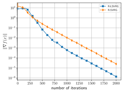
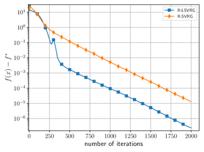
Figure 1: Comparison of the R-LSVRG and R-SVRG methods: Left panel illustrates convergence in terms of gradient norm, while the right panel depicts convergence in terms of function values.

6 Riemannian MARINA

In this section, we consider the finite-sum problem (1) as a distributed optimization problem, where each function $f_{i}(x)$ is stored or located on different workers/machines that collaborate to achieve a common objective. Instead of centralizing the optimization process, it is parallel, with each component handling a portion of the computation. This approach is often employed in large-scale systems, such as distributed computing networks, parallel processing, or decentralized machine learning algorithms. The goal is to enhance efficiency, scalability, and the ability to handle complex tasks by leveraging the computational resources of multiple entities.

We outline another algorithm employed in our study: Riemannian MARINA (refer to Algorithm 3). During each iteration of R-MARINA, each worker i randomly selects between sending the dense vector $\nabla f_{i}(x^{k+1})$ with a probability of $p$ or sending the compressed gradient difference $\mathcal{Q}_{i}\left(\nabla f_{i}(x^{k+1})-\Gamma_{x^{k}}^{x^{k+1}}\nabla f_{i}(x^{k})\right)$ with a probability of $1-p$. In the former scenario, the server simply averages the vectors received from workers to obtain $g^{k+1}=\nabla f\left(x^{k+1}\right)$. Conversely, in the latter case, the server averages the compressed differences from all workers and adds the result to $g^{k}$, yielding $g^{k+1}$.

Next, we delineate an extensive category of unbiased compression operators that adhere to a specific variance constraint.

Definition 3.

We say that a stochastic mapping $Q:T_{x}\mathcal{M}\rightarrow T_{x}\mathcal{M},$ for all $x\in\mathcal{M},$ is a unbiased compression operator/compressor with conic variance if there exists $\omega\geq 0$ such that for any $x\in\mathcal{M},$ any $y\in T_{x}\mathcal{M},$ we have

$$\mathbb{E}\left[Q(y)\right]=y,\quad\mathbb{E}\left[\|Q(y)-y\|^{2}\right]\leq\omega\|y\|^{2}.$$

For the given compressor $Q(y),$ we define the expected density as $\rho_{Q}=\sup_{x\in\mathcal{M},y\in T_{x}\mathcal{M}}\mathbb{E}\left[\|Q(y)\|_{0}\right],$ where $\|z\|_{0}$ is the number of non-zero components of $z\in T_{x}\mathcal{M}.$

Notice that the expected density is well-defined for any compression operator since $\|Q(z)\|_{0}\leq d,$ where $d$ is the local dimension of the manifold. Next, we present the optimal communication complexity for the Riemannian distributed non-convex setting.

Theorem 5.

Assume each $f_{i}$ is $L$-g-smooth on $\mathcal{M}$ (Assumption 3 holds) and let $f$ be uniformly lower bounded on $\mathcal{M}$ (Assumption 5 holds). Assume that the compression operator is unbiased and has conic variance (Definition 3). Let $\delta^{0}\stackrel{{\scriptstyle\text{def}}}{{=}}f(x^{0})-f^{*}$. Select the stepsize $\eta$ such that $\eta\leq\frac{1}{L\left(1+\sqrt{\frac{1-p}{p}\frac{\omega}{n}}\right)}.$ Then, the iterates of the Riemannian MARINA method (Algorithm 3) satisfy

$$\mathbb{E}\left[\|f\left(\widehat{x}^{K}\right)\|^{2}\right]\leq\frac{2\delta^{0}}{\gamma K},$$ (5)

where $\widehat{x}^{K}$ is chosen uniformly at random from $x^{0},\dots,x^{K-1}$.

Corollary 10.

With the assumptions outlined in Theorem 5, if we set $\eta=\frac{1}{L\left(1+\sqrt{\frac{1-p}{p}\frac{\omega}{n}}\right)}$, in order to obtain $\mathbb{E}\left[\|\nabla f\left(\widehat{x}^{K}\right)\|^{2}\right]\leq\varepsilon^{2},$ we find that the communication complexity of Riemannian MARINA method (Algorithm 3) is given by

$$K=\mathcal{O}\left(\frac{\delta^{0}L}{\varepsilon^{2}}\left(1+\sqrt{\frac{(1-p)\omega}{pn}}\right)\right).$$

Corollary 11.

With the assumptions outlined in Theorem 5, if we set $\eta=\frac{1}{L\left(1+\sqrt{\frac{1-p}{p}\frac{\omega}{n}}\right)}$, $p=\frac{\rho_{\mathcal{Q}}}{d}$ in order to obtain $\mathbb{E}\left[\|\nabla f\left(\widehat{x}^{K}\right)\|^{2}\right]\leq\varepsilon^{2},$ we find that the communication complexity $\mathcal{C}$ of Riemannian MARINA method (Algorithm 3) is given by

$$\mathcal{C}=\mathcal{O}\left(\frac{\delta_{0}L}{\varepsilon^{2}}\left(1+\sqrt{\frac{\omega}{n}\left(\frac{d}{\rho_{\mathcal{Q}}}-1\right)}\right)\right),$$

where $\rho_{Q}$ is the expected density of the quantization (see Def. 3) and the expected total communication cost per worker is $\mathcal{O}\left(d+\rho_{\mathcal{Q}}K\right)$.

This signifies that, to the best of our knowledge, we have attained the initial findings for the distributed Riemannian non-convex setting with gradient compression. Our results are consistent with the optimal communication complexity observed in the Euclidean case.

7 Experiments

In this section, we utilize our examination of R-LSVRG to address the problem of fast computation of eigenvectors - a fundamental challenge currently under active investigation in the big-data context (Garber and Hazan, 2015; Jin et al., 2015; Shamir, 2015). Specifically, we have the following problem.

$$\min_{x^{\top}x=1}-x^{\top}\left(\sum_{i=1}^{n}z_{i}z_{i}^{\top}\right)x\stackrel{{\scriptstyle\text{def}}}{{=}}-x^{\top}Ax=f(x),$$

In our experiments, we employ the Pymanopt toolbox for Riemannian optimization in Python (Townsend et al., 2016). We conduct a comparative analysis between the R-LSVRG method (Algorithm 1) and the loop version, which is Riemannian SVRG method. To ensure a fair comparison, we set identical values for the step size, denoted as $\eta$, and the parameter for the inner loop, fixed at $n$ (for R-LVSRG, we utilize $p=1/n$). The results demonstrate a significant improvement of R-LSVRG over R-SVRG.

8 Conclusion

In this study, we examined the loopless variant of the well-known Riemannian SVRG method and demonstrated that replacing the double loop structure with a coin flip mechanism enhances the method both theoretically and empirically. Motivated by this observation, we extended the PAGE method to Riemannian non-convex settings. Our results align with the current state-of-the-art theoretical guarantees, yet they indicate that the analysis can be significantly simplified and made more accessible. Leveraging the R-PAGE method as a foundation, we also obtained, to the best of our knowledge, the initial findings for the distributed Riemannian setting with communication gradient compression through the application of the R-MARINA method. Nevertheless, our analysis does not encompass acceleration mechanisms, a topic deserving a dedicated paper. This aspect is deferred to future work, presenting an avenue of high interest for the scientific community.

Appendix A Extended Related Work

A.1 Riemannian Optimization

References predating this point can be located in works of Udriste (1997, 2013). Stochastic Riemannian optimization has been explored in prior work Liu et al. (2003), albeit with a focus on asymptotic convergence analysis and an absence of specific convergence rates. Boumal et al. (2019) conducted an analysis of the iteration complexity of Riemannian trust-region methods, whereas Bento et al. (2017) delved into the non-asymptotic convergence of Riemannian gradient, subgradient, and proximal point methods. Tripuraneni et al. (2018) investigated aspects beyond variance reduction to expedite the convergence of first-order optimization methods on Riemannian manifolds. In the context of Federated Learning, the Riemannian optimization methods are applicable, as discussed by Li and Ma (2022). Accelerating methods are also widely analysied in Riemannian setting (Martínez-Rubio, 2022; Martínez-Rubio and Pokutta, 2023)

A.2 Variance Reduction

Reducing variance in stochastic optimization involves employing various techniques. Control variates, a common method used in Monte Carlo simulations, are among the widely adopted variance reduction techniques (Haghighat and Wagner, 2003; Rubinstein and Kroese, 2016). There has been a notable upswing in interest recently regarding variance-reduced methods for solving finite-sum problems in linear spaces (J Reddi et al., 2015; Hanzely et al., 2018; Malinovsky and Richtárik, 2022; Hanzely et al., 2020; Shang et al., 2018; Malinovsky et al., 2022). Furthermore, there is extensive analysis of acceleration techniques incorporating Nesterov momentum (Nesterov, 1983) with variance reduction (Allen-Zhu, 2018a, b; Qian et al., 2021a; Xu and Xu, 2021; Condat et al., 2023; Grudzień et al., 2023). In the context of sampling without replacement (random reshuffling), researchers have also investigated variance reduction (Ying et al., 2020; Huang et al., 2021; Malinovsky et al., 2023b). In the realm of non-convex optimization, researchers actively explore a multitude of strategies and methodologies for mitigating variance, a crucial aspect in the optimization process (Cutkosky and Orabona, 2019; Liu et al., 2017; Kavis et al., 2022).

A.3 Communication Compression

In a distributed setting, various compression schemes are extensively studied to enhance the communication efficiency of methods (Seide et al., 2014; Wen et al., 2017; Ivkin et al., 2019; Tang et al., 2021; Sattler et al., 2019). The investigation and incorporation of variance reduction mechanisms into compression and acceleration techniques represent an area of extensive research. Researchers are actively exploring diverse strategies and methodologies aimed at refining compression (Sadiev et al., 2022) and acceleration techniques (Li et al., 2020; Yang et al., 2021). In the context of biased compression, the error feedback mechanism (Karimireddy et al., 2019) is extensively analyzed and has been demonstrated to be effectively combined with acceleration (Qian et al., 2021b). In a non-convex setting, variance reduction mechanisms are explored within the MARINA method, as discussed by Gorbunov et al. (2021). Additionally, several enhancements derived from the MARINA method are presented in several works (Szlendak et al., 2021; Panferov et al., 2024; Tyurin and Richtárik, 2022). In the context of Byzantine robustness, the MARINA method has been thoroughly analyzed (Gorbunov et al., 2023; Malinovsky et al., 2023a; Rammal et al., 2023).

Appendix B R-LSVRG: Strongly Convex Case

Theorem 1. Assuming that in (1), each $f_{i}$ is differentiable and $L$-g-smooth on $\mathcal{X}$ (Assumption 3 holds), and $f$ is $\mu$-strongly g-convex on $\mathcal{X}$ (Assumption 2 holds). Additionally, let Assumption 6 hold. Choose the stepsize $0<\eta\leq\frac{\mu}{16L^{2}\zeta}.$ Then, the iterates of the Riemannian L-SVRG method (Algorithm 1) satisfy

$$\mathbb{E}\left[\Phi^{k}\right]\leq\left(\max\left\{1-\eta\mu,1-\frac{p}{2}\right\}\right)^{k}\Phi^{0},$$

where $\Phi^{k}\stackrel{{\scriptstyle\text{def}}}{{=}}d^{2}\left(x^{k},x^{*}\right)+\frac{3\mu^{2}}{64pL^{2}\zeta}\mathcal{D}^{k}$ and $\mathcal{D}^{k}\stackrel{{\scriptstyle\text{def}}}{{=}}\left\|\mathrm{Exp}^{-1}_{y^{k}}(x^{*})\right\|^{2}.$

Proof of Theorem 1.

Conditioned on $x^{k},$ take expectation with respect to $i:$

$$\begin{split}{\mathbb{E}}\left[\left\|g^{k}\right\|^{2}\right]&={\mathbb{E}}\left[\left\|\frac{1}{B}\sum_{i\in I}\left(\nabla f_{i}(x^{k})-\Gamma_{y^{k}}^{x^{k}}\nabla f_{i}(y^{k})\right)+\Gamma_{y^{k}}^{x^{k}}\nabla f(y^{k})\right\|^{2}\right]\\ &={\mathbb{E}}\left[\left\|\frac{1}{B}\sum_{i\in I}\left(\nabla f_{i}(x^{k})-\Gamma_{y^{k}}^{x^{k}}\nabla f_{i}(y^{k})\right)+\Gamma_{y^{k}}^{x^{k}}\left(\nabla f(y^{k})-\Gamma_{x^{*}}^{y^{k}}\nabla f(x^{*})\right)\right\|^{2}\right]\\ &\leq 2{\mathbb{E}}\left[\left\|\frac{1}{B}\sum_{i\in I}\left(\nabla f_{i}(x^{k})-\Gamma_{y^{k}}^{x^{k}}\nabla f_{i}(y^{k})\right)\right\|^{2}\right]+2{\mathbb{E}}\left[\left\|\nabla f(y^{k})-\Gamma_{x^{*}}^{y^{k}}\nabla f(x^{*})\right\|^{2}\right]\\ &\leq 2L^{2}\left\|\mathrm{Exp}^{-1}_{x^{k}}(y^{k})\right\|^{2}+2L^{2}\left\|\mathrm{Exp}^{-1}_{y^{k}}(x^{*})\right\|^{2}\\ &\leq 2L^{2}\left(\left\|\mathrm{Exp}^{-1}_{x^{k}}(x^{*})\right\|+\left\|\mathrm{Exp}^{-1}_{y^{k}}(x^{*})\right\|\right)^{2}+2L^{2}\left\|\mathrm{Exp}^{-1}_{y^{k}}(x^{*})\right\|^{2}\\ &\leq 4L^{2}\left\|\mathrm{Exp}^{-1}_{x^{k}}(x^{*})\right\|^{2}+6L^{2}\left\|\mathrm{Exp}^{-1}_{y^{k}}(x^{*})\right\|^{2}.\end{split}$$

We use the definition of $g^{k}$ from Algorithm 1, the fact that $\nabla f(x^{*})=0,$ the Young’s inequality and the fact that the parallel transport preserves the scalar product, $L$-g-smoothness of $f(x),$ the triangle inequality, the Young’s inequality.

Let us define $\mathcal{D}^{k}\stackrel{{\scriptstyle\text{def}}}{{=}}\left\|\mathrm{Exp}^{-1}_{y^{k}}(x^{*})\right\|^{2}.$ Notice that

$$\begin{split}{\mathbb{E}}\left[\mathcal{D}^{k+1}\right]&=p\left\|\mathrm{Exp}^{-1}_{x^{k}}(x^{*})\right\|^{2}+\left(1-p\right)\left\|\mathrm{Exp}^{-1}_{y^{k}}(x^{*})\right\|^{2}\\ &=pd^{2}(x^{k},x^{*})+(1-p)\mathcal{D}^{k}.\\ \end{split}$$ (6)

Further, we have

$$\begin{split}{\mathbb{E}}\left[d^{2}(x^{k+1},x^{*})\right]&\leq d^{2}(x^{k},x^{*})+2\eta\langle\mathrm{Exp}^{-1}_{x^{k}}(x^{*}),{\mathbb{E}}\left[g^{k}\right]\rangle+\zeta\eta^{2}{\mathbb{E}}\left[\left\|g^{k}\right\|^{2}\right]\\ &\leq d^{2}(x^{k},x^{*})+2\eta\langle\mathrm{Exp}^{-1}_{x^{k}}(x^{*}),\nabla f(x^{k})\rangle\\ &+\zeta\eta^{2}\left(4L^{2}\left\|\mathrm{Exp}^{-1}_{x^{k}}(x^{*})\right\|^{2}+6L^{2}\left\|\mathrm{Exp}^{-1}_{y^{k}}(x^{*})\right\|^{2}\right)\\ &\leq\left(1-\eta\mu+4L^{2}\eta^{2}\zeta\right)d^{2}(x^{k},x^{*})+2\eta\left(f(x^{*})-f(x^{k})\right)\\ &+6L^{2}\eta^{2}\zeta\mathcal{D}^{k}.\end{split}$$

We use Corollary 1, bound on ${\mathbb{E}}\left[\left\|g^{k}\right\|^{2}\right],$ strong convexity.

Observe that due to $g$-strong convexity we also have that

$$f(x^{k})-f(x^{*})\geq\langle\nabla f(x^{*}),\mathrm{Exp}^{-1}_{x^{k}}(x^{*})\rangle-\frac{\mu}{2}d^{2}\left(x^{k},x^{*}\right)=-\frac{\mu}{2}d^{2}\left(x^{k},x^{*}\right).$$

Therefore, we obtain that

$$\begin{split}{\mathbb{E}}\left[d^{2}(x^{k+1},x^{*})\right]&\leq\left(1-2\eta\mu+4L^{2}\eta^{2}\zeta\right)d^{2}(x^{k},x^{*})+6L^{2}\eta^{2}\zeta\mathcal{D}^{k}.\end{split}$$

Multiply both sides of (6) by $\frac{12L^{2}\eta^{2}\zeta}{p},$ and add it to the last equation:

$$\begin{split}{\mathbb{E}}\left[d^{2}(x^{k+1},x^{*})\right]+\frac{12L^{2}\eta^{2}\zeta}{p}{\mathbb{E}}\left[\mathcal{D}^{k+1}\right]&\leq\left(1-2\eta\mu+16L^{2}\eta^{2}\zeta\right)d^{2}(x^{k},x^{*})\\ &+\frac{12L^{2}\eta^{2}\zeta}{p}\left(1-\frac{p}{2}\right)\mathcal{D}^{k}.\end{split}$$

Define the Lyapunov funciton $\Phi^{k}\stackrel{{\scriptstyle\text{def}}}{{=}}d^{2}\left(x^{k},x^{*}\right)+\frac{12L^{2}\eta^{2}\zeta}{p}\mathcal{D}^{k}.$ Then we have that

$${\mathbb{E}}\left[\Phi^{k+1}\right]\leq\max\left\{1-2\eta\mu+16L^{2}\eta^{2}\zeta,1-\frac{p}{2}\right\}\Phi^{k}.$$

Due to the choice of $\eta=\frac{\mu}{16L^{2}\zeta},$ it follows that $1-2\eta\mu+16L^{2}\eta^{2}\zeta=1-\frac{\mu^{2}}{16L^{2}\zeta}.$ Unrolling the recursion, we arrive at

$${\mathbb{E}}\left[\Phi^{k}\right]\leq\left(\max\left\{1-\frac{\mu^{2}}{16L^{2}\zeta},1-\frac{p}{2}\right\}\right)^{k}\Phi^{0}.$$

∎

Corollary 2. With the assumptions outlined in Theorem 1, if we set $\eta=\frac{\mu}{16L^{2}\zeta}$, in order to obtain $\mathbb{E}[\Phi^{k}]\leq\varepsilon\Phi^{0}$, we find that the iteration complexity of Riemannian L-SVRG method (Algorithm 1) is given by

$$K=\mathcal{O}\left(\left(\frac{1}{p}+\frac{L^{2}\zeta}{\mu^{2}}\right)\log\frac{1}{\varepsilon}\right).$$

Proof of Corollary 2.

Observe that

$$\left(1-\frac{\mu^{2}}{16L^{2}\zeta}\right)^{k}\leq e^{-\frac{k\mu^{2}}{16L^{2}\zeta}},\quad\left(1-\frac{p}{2}\right)^{k}\leq e^{-\frac{kp}{2}}.$$

Now the result simply follows from (3). ∎

Corollary 3. With the assumptions outlined in Theorem 1, if we set $\eta=\frac{\mu}{16L^{2}\zeta}$ and $p=\frac{1}{n}$, in order to obtain $\mathbb{E}[\Phi^{k}]\leq\varepsilon\Phi^{0}$, we find that the total computational complexity of Riemannian L-SVRG method (Algorithm 1) is given by

$$K=\mathcal{O}\left(\left(n+\frac{L^{2}\zeta}{\mu^{2}}\right)\log\frac{1}{\varepsilon}\right).$$

Proof of Corollary 3.

Choose $B=1.$ Riemannian L-SVRG calls the stochastic gradient oracle in expectation $\mathcal{O}(1+pn)$ times in each iteration. Corollary 6 states that the iteration complexity is $\mathcal{O}\left(\left(\frac{1}{p}+\frac{L^{2}\zeta}{\mu^{2}}\right)\log\frac{1}{\varepsilon}\right).$ Note that any choice of

$$p\in\left[\min\left\{\frac{\mu^{2}}{L^{2}\zeta},\frac{1}{n}\right\},\max\left\{\frac{\mu^{2}}{L^{2}\zeta},\frac{1}{n}\right\}\right]$$

leads to the total complexity of $\mathcal{O}\left(\left(n+\frac{L^{2}\zeta}{\mu^{2}}\right)\log\frac{1}{\varepsilon}\right).$ The choice of $p=\frac{1}{n}$ is motivated by the lack of dependence on $L$ and $\mu.$ ∎

Appendix C R-PAGE: SOTA non-convex Optimization Algorithm

Theorem 2. Assuming that each $f_{i}$ in (1) is differentiable and $L$-g-smooth on $\mathcal{M}$ (Assumption 3 holds) and that $f$ is lower bounded on $\mathcal{M}$ (Assumption 5 holds), let $\delta^{0}\stackrel{{\scriptstyle\text{def}}}{{=}}f(x^{0})-f^{*}$. Select the stepsize $\eta$ such that $0<\eta\leq\frac{1}{L\left(1+\sqrt{\frac{1-p}{pb}}\right)},$ and the minibatch size $B=n,$ and the secondary minibatch size $b<B.$ Then, the iterates of the R-PAGE method (Algorithm 2) satisfy

$$\mathbb{E}\left[\left\|\nabla f(\widehat{x}^{K})\right\|^{2}\right]\leq\frac{2\delta^{0}}{\eta K},$$

where $\widehat{x}^{k}$ is chosen randomly from $x^{0},\ldots,x^{K-1}$ with uniform probability distribution.

Proof of Theorem 2.

Let $X=g^{k}-\nabla f(x^{k}),$ $a_{i}=\nabla f_{i}\left(x^{k+1}\right)-\Gamma_{x^{k}}^{x^{k+1}}\nabla f_{i}\left(x^{k}\right).$ A direct calculation now reveals that

$$\begin{split}G&\stackrel{{\scriptstyle\text{def}}}{{=}}\mathbb{E}\left[\left\|g^{k+1}-\nabla f\left(x^{k+1}\right)\right\|^{2}\bigg{|}x^{k+1},x^{k},g^{k}\right]\\ &=p\left\|\nabla f\left(x^{k+1}\right)-\nabla f\left(x^{k+1}\right)\right\|^{2}\\ &+(1-p)\left\|\Gamma_{x^{k}}^{x^{k+1}}g^{k}+\frac{1}{b}\sum_{i\in I}\left(\nabla f_{i}\left(x^{k+1}\right)-\Gamma_{x^{k}}^{x^{k+1}}\nabla f_{i}\left(x^{k}\right)\right)-\nabla f\left(x^{k+1}\right)\right\|^{2}\\ &=(1-p)\left\|\Gamma_{x^{k}}^{x^{k+1}}g^{k}-\Gamma_{x^{k}}^{x^{k+1}}\nabla f\left(x^{k}\right)+\frac{1}{b}\sum_{i\in I}\left(\nabla f_{i}\left(x^{k+1}\right)-\Gamma_{x^{k}}^{x^{k+1}}\nabla f_{i}\left(x^{k}\right)\right)\right.\\ &-\left.\left(\nabla f\left(x^{k+1}\right)-\Gamma_{x^{k}}^{x^{k+1}}\nabla f\left(x^{k}\right)\right)\right\|^{2}\\ &=(1-p)\left\|X\right\|^{2}+2(1-p)\left\langle X,\,\frac{1}{b}\sum_{i\in I}a_{i}-\bar{a}\right\rangle+(1-p)\left\|\frac{1}{b}\sum_{i\in I}a_{i}-\bar{a}\right\|^{2},\end{split}$$

where $\bar{a}=\frac{1}{n}\sum_{i=1}^{n}a_{i}.$

Since $\mathbb{E}\left[a_{i}-\bar{a}\bigg{|}x^{k+1},x^{k},g^{k}\right]=0$ and because $X$ is constant conditioned on $x^{k+1},x^{k},g^{k},$ we have

$$\mathbb{E}\left[G\bigg{|}x^{k+1},x^{k},g^{k}\right] = (1-p)\mathbb{E}\left[\left\|X\right\|^{2}\bigg{|}x^{k+1},x^{k},g^{k}\right]+(1-p){\mathbb{E}}\left[\left\|a_{i}-\bar{a}\right\|^{2}\right]$$

$$= (1-p)\mathbb{E}\left[\left\|X\right\|^{2}\bigg{|}x^{k+1},x^{k},g^{k}\right]+(1-p)\frac{n-b}{(n-1)b}\frac{1}{n}\sum_{i=1}^{n}\left\|a_{i}-\bar{a}\right\|^{2}$$

$$\leq (1-p)\mathbb{E}\left[\left\|X\right\|^{2}\bigg{|}x^{k+1},x^{k},g^{k}\right]+\frac{(1-p)L^{2}}{b}\left\|\mathrm{Exp}_{x^{k}}^{-1}(x^{k+1})\right\|^{2},$$

where in the second step we simply calculate the expectation with respect to the random index, and the last step is due to the smoothness assumption (Assumption 3).

By first applying the three term tower property and subsequently the standard two-term tower property, we get

$$\mathbb{E}\left[\left\|g^{k+1}-\nabla f(x^{k+1})\right\|^{2}\right]$$

$$=\mathbb{E}\left[\mathbb{E}\left[\mathbb{E}\left[\left\|g^{k+1}-\nabla f(x^{k+1})\right\|^{2}\bigg{|}x^{k+1},x^{k},g^{k},s^{k}\right]\bigg{|}x^{k+1},x^{k},g^{k}\right]\right]$$

$$=\mathbb{E}\left[\mathbb{E}\left[G\bigg{|}x^{k+1},x^{k},g^{k}\right]\right]$$

$$\leq\mathbb{E}\left[(1-p)\mathbb{E}\left[\left\|X\right\|^{2}\bigg{|}x^{k+1},x^{k},g^{k}\right]+\frac{(1-p)L^{2}}{b}\mathbb{E}\left[\left\|\mathrm{Exp}_{x^{k}}^{-1}(x^{k+1})\right\|^{2}\right]\right]$$

$$=(1-p)\mathbb{E}\left[\mathbb{E}\left[\left\|X\right\|^{2}\bigg{|}x^{k+1},x^{k},g^{k}\right]\right]+\frac{(1-p)L^{2}}{b}\mathbb{E}\left[\left\|\mathrm{Exp}_{x^{k}}^{-1}(x^{k+1})\right\|^{2}\right]$$

$$=(1-p)\mathbb{E}\left[\left\|X\right\|^{2}\right]+\frac{(1-p)L^{2}}{b}\mathbb{E}\left[\left\|\mathrm{Exp}_{x^{k}}^{-1}(x^{k+1})\right\|^{2}\right]$$

$$=(1-p)\mathbb{E}\left[\left\|g^{k}-\nabla f(x^{k})\right\|^{2}\right]+\frac{(1-p)L^{2}}{b}\mathbb{E}\left[\left\|\mathrm{Exp}_{x^{k}}^{-1}(x^{k+1})\right\|^{2}\right].$$ (7)

Let $x\in\mathcal{M},$ $g\in T_{x}\mathcal{M}.$ By Lemma 4 with $M=L,$ we have the identity

$$\langle\nabla f(x),-\eta g\rangle+\frac{M\eta^{2}}{2}\|g\|^{2} = -\frac{\eta}{2}\|\nabla f(x)\|^{2}-\left(\frac{1}{2\eta}-\frac{M}{2}\right)\|-\eta g\|^{2}$$ (8)

$$+ \frac{\eta}{2}\|g-\nabla f(x)\|^{2}.$$

Since $f$ is $L$-g-smooth, we have

$$f(x^{k+1}) \leq f(x^{k})+\langle\nabla f(x^{k}),\mathrm{Exp}_{x^{k}}^{-1}(x^{k+1})\rangle+\frac{L}{2}\|\mathrm{Exp}_{x^{k}}^{-1}(x^{k+1})\|^{2}]$$

$$\leq \;f(x^{k})-\eta\langle\nabla f(x^{k}),g^{k}\rangle+\frac{L\eta^{2}}{2}\|g^{k}\|^{2}.$$

Subtracting $f^{*}$ from both sides, taking expectation and applying (8), we get

$$\mathbb{E}\left[f(x^{k+1})-f^{*}\right] \leq \mathbb{E}\left[f(x^{k})-f^{*}\right]-\frac{\eta}{2}\mathbb{E}\left[\left\|\nabla f(x^{k})\right\|^{2}\right]$$

$$- \left(\frac{1}{2\eta}-\frac{L}{2}\right)\mathbb{E}\left[\left\|\mathrm{Exp}_{x^{k}}^{-1}(x^{k+1})\right\|^{2}\right]+\frac{\eta}{2}{\mathbb{E}}\left[\left\|g^{k}-\nabla f(x^{k})\right\|^{2}\right].$$

Let $\delta^{k}\stackrel{{\scriptstyle\text{def}}}{{=}}\mathbb{E}[f(x^{k})-f^{*}]$, $s^{k}\stackrel{{\scriptstyle\text{def}}}{{=}}\mathbb{E}[\|g^{k}-\nabla f(x^{k})\|^{2}]$ and $r^{k}\stackrel{{\scriptstyle\text{def}}}{{=}}\mathbb{E}[\|\mathrm{Exp}_{x^{k}}^{-1}(x^{k+1})\|^{2}]$. Then by adding (C) with a $\frac{\eta}{2p}$ multiple of (C), we obtain

$$\delta^{k+1}+\frac{\eta}{2p}s^{k+1}$$

$$\leq\delta^{k}-\frac{\eta}{2}{\mathbb{E}}\left[\|\nabla f(x^{k})\|^{2}\right]-\left(\frac{1}{2\eta}-\frac{L}{2}\right)r^{k}+\frac{\eta}{2}s^{k}+\frac{(1-p)\eta L^{2}}{2pb}r^{k}+\frac{\eta}{2p}(1-p)s^{k}$$

$$=\delta^{k}+\frac{\eta}{2p}s^{k}-\frac{\eta}{2}{\mathbb{E}}\left[\|\nabla f(x^{k})\|^{2}\right]-\left(\frac{1}{2\eta}-\frac{L}{2}-\frac{(1-p)\eta L^{2}}{2pb}\right)r^{k}$$

$$\leq\delta^{k}+\frac{\eta}{2p}s^{k}-\frac{\eta}{2}{\mathbb{E}}\left[\|\nabla f(x^{k})\|^{2}\right].$$ (10)

The last inequality follows from the bound $\frac{(1-p)L^{2}}{pb}\eta^{2}+L\eta\leq 1$, which holds due to the choice of stepsize and Lemma 3.

By summing up inequalities (C) for $k=0,\ldots,K-1$, we get

$$0\leq\delta^{K}+\frac{\eta}{2p}s^{K}\leq\delta^{0}+\frac{\eta}{2p}s^{0}-\frac{\eta}{2}\sum_{k=0}^{K-1}\mathbb{E}[\|\nabla f(x^{k})\|^{2}].$$

Since $g^{0}=\nabla f(x^{0}),$ we have that $s^{0}=0.$ We get that

$${\mathbb{E}}\left[\left\|\nabla f(\widehat{x}^{K})\right\|^{2}\right]=\frac{1}{K}\sum_{k=0}^{K-1}{\mathbb{E}}\left[\left\|\nabla f(x^{k})\right\|^{2}\right]\leq\frac{2\delta^{0}}{\eta K}.$$

∎

Corollary 4. With the assumptions outlined in Theorem 2, if we set $\eta=\frac{1}{L\left(1+\sqrt{\frac{1-p}{pb}}\right)}$, in order to obtain $\mathbb{E}\left[\left\|\nabla f\left(\widehat{x}^{K}\right)\right\|\right]\leq\varepsilon$, we find that the iteration complexity of Riemannian R-PAGE method (Algorithm 2) is given by

$$K=\mathcal{O}\left(\left(1+\sqrt{\frac{1-p}{pb}}\right)\frac{L\delta^{0}}{\varepsilon^{2}}\right).$$

Proof of Corollary 4.

Let $\eta=\frac{1}{L\left(1+\sqrt{\frac{1-p}{pb}}\right)}.$ Then ${\mathbb{E}}\left[\left\|\nabla f\left(\widehat{x}^{K}\right)\right\|^{2}\right]\leq\varepsilon^{2}$ as long as $K\geq\frac{2\left(1+\sqrt{\frac{1-p}{pb}}\right)L\delta^{0}}{\varepsilon^{2}}.$ ∎

Corollary 5. With the assumptions outlined in Theorem 2, if we set $\eta=\frac{1}{L\left(1+\sqrt{\frac{1-p}{pb}}\right)}$, minibatch size $B=n$, secondary minibatch size $b\leq\sqrt{B}$ and $p\equiv\frac{b}{B+b}$, in order to obtain $\mathbb{E}\left[\left\|\nabla f\left(\widehat{x}^{K}\right)\right\|\right]\leq\varepsilon$, we find that the total computational complexity of Riemannian PAGE method (Algorithm 2) is given by

$$\#\operatorname{grad}=\mathcal{O}\left(n+\frac{\sqrt{n}}{\varepsilon^{2}}\right).$$

Proof of Corollary 5.

At each iteration, R-PAGE computes $(1-p)b+pn$ new gradients on average. Note that in the preprocessing step $n$ gradients $\nabla f_{1}(x^{0}),\ldots,\nabla f_{n}(x^{0})$ are computed. Therefore, the total expected number of gradients computed by R-PAGE in order to reach an $\varepsilon$-accurate solution is

$$\#\operatorname{grad} =n+\left\lceil\frac{2L\delta^{0}\left(1+\sqrt{\frac{1-p}{pb}}\right)}{\varepsilon^{2}}-1\right\rceil\left((1-p)b+pn\right)$$

$$\leq n+\frac{2L\delta^{0}\left(1+\sqrt{\frac{1-p}{pb}}\right)}{\varepsilon^{2}}\left((1-p)b+pn\right)$$

$$=\mathcal{O}\left(n+\frac{\sqrt{n}}{\varepsilon^{2}}\right).$$

∎

Appendix D R-PAGE: SOTA Algorithm Under PL-Condition

Theorem 3. Assuming that each $f_{i}$ in (1) is differentiable and $L$-g-smooth on $\mathcal{M}$ (Assumption 3 holds), also that $f$ is lower bounded on $\mathcal{M}$ (Assumption 5 holds) and it satisfies Polyak-Łojasiewicz condition (Assumption 4 holds) with constant $\mu$, let $\delta^{0}\stackrel{{\scriptstyle\text{def}}}{{=}}f(x^{0})-f^{*}$. Select the stepsize $\eta$ such that $\eta\leq\min\left\{\frac{1}{L\left(1+\sqrt{\frac{1-p}{pb}}\right)},\frac{p}{2\mu}\right\}.$ Then, the iterates of the Riemannian PAGE method (Algorithm 2) satisfy

$$\mathbb{E}\left[\Phi^{K}\right]\leq(1-\mu\eta)^{K}\delta^{0},$$

where $\Phi^{k}\stackrel{{\scriptstyle\text{def}}}{{=}}f\left(x^{k}\right)-f^{*}+\frac{2}{p}\left\|g^{k}-\nabla f\left(x^{k}\right)\right\|^{2}$ and $\Phi^{0}=\delta^{0}$, since $g^{0}=\nabla f(x^{0}).$

Proof of Theorem 3..

Add $\beta\times$ (C) to (C), we get

$$\mathbb{E}[\nabla f(x^{k+1})-f^{*}+\beta\|g^{k+1}-\nabla f(x^{k+1})\|^{2}]$$

$$\leq\mathbb{E}\left[(1-\mu\eta)(f(x^{k})-f^{*})-\left(\frac{1}{2\eta}-\frac{L}{2}\right)\|\mathrm{Exp}_{x^{k}}^{-1}(x^{k+1})\|^{2}+\frac{\eta}{2}\|g^{k}-\nabla f(x^{k})\|^{2}\right]$$

$$\quad+\beta\mathbb{E}\left[(1-p)\|g^{k}-\nabla f(x^{k})\|^{2}+\frac{(1-p)L^{2}}{b}\|\mathrm{Exp}_{x^{k}}^{-1}(x^{k+1})\|^{2}\right]$$

$$=\mathbb{E}\left[(1-\mu\eta)(f(x^{k})-f^{*})+\left(\frac{\eta}{2}+(1-p)\beta\right)\|g^{k}-\nabla f(x^{k})\|^{2}\right.$$

$$\left.\quad-\left(\frac{1}{2\eta}-\frac{L}{2}-\frac{(1-p)\beta L^{2}}{b}\right)\|\mathrm{Exp}_{x^{k}}^{-1}(x^{k+1})\|^{2}\right]$$

$$\leq\mathbb{E}\left[(1-\mu\eta)(f(x^{k})-f^{*}+\beta\|g^{k}-\nabla f(x^{k})\|^{2})\right],$$ (11)

where the last inequality holds by choosing the stepsize

$$\eta\leq\min\left\{\frac{p}{2\mu},\frac{1}{L\left(1+\sqrt{\frac{1-p}{pb}}\right)}\right\},$$

and $\beta\geq\frac{2}{p}$. Now, we define $\Phi^{k}:=f(x^{k})-f^{*}+\beta\|g^{k}-\nabla f(x^{k})\|^{2}$, then (D) turns to

$$\mathbb{E}[\Phi^{k+1}]\leq(1-\mu\eta)\mathbb{E}[\Phi^{k}].$$

Telescoping it for $k=0,\ldots,K-1$, we have

$$\mathbb{E}[\Phi^{K}]\leq(1-\mu\eta)^{K}\mathbb{E}[\Phi^{0}].$$

∎

Corollary 6. With the assumptions outlined in Theorem 3, if we set $\eta=\min\left\{\frac{1}{L\left(1+\sqrt{\frac{1-p}{pb}}\right)},\frac{p}{2\mu}\right\}$, in order to obtain $\mathbb{E}[\Phi^{k}]\leq\varepsilon\Phi^{0}$, we find that the iteration complexity of Riemannian R-PAGE method (Algorithm 2) is given by

$$K=\mathcal{O}\left(\left(\left(1+\sqrt{\frac{1-p}{pb}}\right)\frac{L}{\mu}+\frac{1}{p}\right)\log\frac{1}{\varepsilon}\right).$$

Proof of Corollary 6.

Note that $\Phi^{0}=f(x^{0})-f^{*}+\beta\|g^{0}-\nabla f(x^{0})\|^{2}=f(x^{0})-f^{*}\stackrel{{\scriptstyle\text{def}}}{{=}}\delta^{0}$, we have

$$\mathbb{E}[f(x^{K})-f^{*}]\leq(1-\mu\eta)^{K}\delta^{0}=\varepsilon,$$

where the last equality holds due to the choice of the number of iterations

$$K=\frac{1}{\mu\eta}\log\frac{\delta^{0}}{\varepsilon}=\left(\left(1+\sqrt{\frac{1-p}{pb}}\right)\kappa+\frac{2}{p}\right)\log\frac{\delta^{0}}{\varepsilon},$$

where $\kappa:=\frac{L}{\mu}$. ∎

Now, we restate the corollary, in which a detailed convergence result is obtained by giving a specific parameter setting, and then provide its proof.

Corollary 7. Suppose that each $f_{i}$ satisfies Assumption 3 with constant $L\geq 0$ and Assumption 4 holds for $f$ with constant $\mu>0.$ Let stepsize

$$\eta\leq\min\left\{\frac{1}{L\left(1+\frac{\sqrt{n}}{b}\right)},\frac{b}{2\mu(n+b)}\right\},$$

and probability $p=\frac{b}{n+b}.$ Then the number of iterations performed by R-PAGE to find an $\varepsilon$-solution of non-convex finite-sum problem (1) can be bound by $K=\left(\left(1+\frac{\sqrt{n}}{b}\right)\kappa+\frac{2(n+b)}{b}\right)\log\frac{\delta^{0}}{\varepsilon}.$ Moreover, the number of stochastic gradient computations (gradient complexity) is

$$\#grad\leq n+\left(4\sqrt{n}\kappa+4n\right)\log\frac{\delta^{0}}{\varepsilon}=\mathcal{O}\left((n+\sqrt{n}\kappa)\log\frac{1}{\varepsilon}\right).$$

Proof of Corollary 7..

If we choose probability $p=\frac{b}{n+b}$, then the term $\sqrt{\frac{1-p}{pb}}$ becomes $\frac{\sqrt{n}}{b}.$ Thus, according to Theorem 3, the stepsize is

$$\eta\leq\min\left\{\frac{1}{L\left(1+\frac{\sqrt{n}}{b}\right)},\frac{b}{2\mu(n+b)}\right\},$$

and the total number of iterations $K=\left(\left(1+\frac{\sqrt{n}}{b}\right)\kappa+\frac{2(n+b)}{b}\right)\log\frac{\delta^{0}}{\varepsilon}.$

According to the gradient estimator of R-PAGE (Line 5 of Algorithm 2), we know that it uses $pn+(1-p)b=\frac{2nb}{n+b}$ stochastic gradients for each iteration on the expectation. Thus, the gradient complexity

$$\#grad =n+K(pn+(1-p)b)$$

$$=n+\frac{2n}{n+1}\left(\left(1+\frac{\sqrt{n}}{b}\right)\kappa+\frac{2(n+b)}{b}\right)\log\frac{\delta^{0}}{\varepsilon}$$

$$=n+\left(\frac{2nb}{n+b}\left(1+\frac{\sqrt{n}}{b}\right)\kappa+4n\right)\log\frac{\delta^{0}}{\varepsilon}$$

$$\leq n+\left(2b\left(1+\frac{\sqrt{n}}{B}\right)\kappa+4n\right)\log\frac{\delta^{0}}{\varepsilon}$$

$$\leq n+\left(4\sqrt{n}\kappa+4n\right)\log\frac{\delta^{0}}{\varepsilon}$$

$$=\mathcal{O}\left(\left(n+\sqrt{n}\kappa\right)\log\frac{1}{\varepsilon}\right).$$

∎

Appendix E R-PAGE: Online non-convex Case

In this appendix, we provide the detailed proofs for our main convergence theorem and its corollaries for R-PAGE in the non-convex online case (i.e., problem (4)).

We first restate the main convergence result (Theorem 4) in the non-convex online case and then provide its proof.

Theorem 4. Suppose that Assumption 7 and Assumption 8 hold for the stochastic gradient $\nabla f_{B}(x)$ and suppose that, for any fixed $\xi_{i},$ $f(x,\xi_{i})$ is geodesically $L$-smooth on $\mathcal{M}$ (Assumption 3 holds), also that $f$ is lower bounded on $\mathcal{M}$ (Assumption 5 holds). Let $\delta^{0}\stackrel{{\scriptstyle\text{def}}}{{=}}f(x^{0})-f^{*}$. Select the stepsize $\eta$ such that $\eta\leq\frac{1}{L\left(1+\sqrt{\frac{1-p}{pb}}\right)}.$ Then, the iterates of the Riemannian PAGE method (Algorithm 2) satisfy

$$\mathbb{E}\|\nabla f(\widehat{x}^{K})\|^{2}\leq\frac{2\mathbb{E}[\Phi^{0}]}{\eta K}+\frac{\sigma^{2}}{B}.$$

where $\widehat{x}^{K}$ is chosen uniformly at random from $x^{0},\dots,x^{K-1}$ and $\Phi^{0}=f\left(x^{0}\right)-f^{*}+\frac{\eta\sigma^{2}}{2pB}$

Proof of Theorem 4.

According to the update step $x^{k+1}=\mathrm{Exp}_{x^{k}}\left(-\eta g^{k}\right)$ (see Line 4 in Algorithm 2) and (C), we have

$$f(x^{k+1})\leq f(x^{k})-\frac{\eta}{2}\|\nabla f(x^{k})\|^{2}-\left(\frac{1}{2\eta}-\frac{L}{2}\right)\left\|\mathrm{Exp}_{x^{k}}^{-1}\left(x^{k+1}\right)\right\|^{2}+\frac{\eta}{2}\|g^{k}-\nabla f(x^{k})\|^{2}.$$ (12)

Now, we use the following Lemma 2 to bound the last term.

Lemma 2.

Suppose that Assumption 7 holds for the stochastic gradient $\nabla f_{B}(x)$ and suppose that, for any fixed $\xi_{i},$ $f(x,\xi_{i})$ is geodesically $L$-smooth in $x\in\mathcal{M}.$ If the gradient estimator $g^{k+1}$ is defined in Line 5 of Algorithm 2, then we have

$$\mathbb{E}\left[\|g^{k+1}-\nabla f(x^{k+1})\|^{2}\right]\leq(1-p)\|g^{k}-\nabla f(x^{k})\|^{2}+\frac{(1-p)L^{2}}{b}\left\|\mathrm{Exp}_{x^{k}}^{-1}(x^{k+1})\right\|^{2}+\frac{p\sigma^{2}}{B}.$$ (13)

Proof of Lemma 2.

According to the definition of R-PAGE gradient estimator in Line 5 of Algorithm 2

$$g^{k+1}=\begin{cases}\nabla f_{B}(x^{k+1})&\text{with probability }p,\\ \Gamma_{x^{k}}^{x^{k+1}}g^{k}+\nabla f_{b}(x^{k+1})-\Gamma_{x^{k}}^{x^{k+1}}\nabla f_{b}(x^{k})&\text{with probability }1-p,\end{cases}$$

we have

$${\mathbb{E}}\left[\left\|g^{k+1}-\nabla f(x^{k+1})\right\|^{2}\right]$$

$$=p{\mathbb{E}}\left[\left\|\nabla f_{B}(x^{k+1})-\nabla f(x^{k+1})\right\|^{2}\right]$$

$$+(1-p){\mathbb{E}}\left[\left\|\Gamma_{x^{k}}^{x^{k+1}}g^{k}+\nabla f_{b}(x^{k+1})-\Gamma_{x^{k}}^{x^{k+1}}\nabla f_{b}(x^{k})-\nabla f(x^{k+1})\right\|^{2}\right]$$

$$\stackrel{{\scriptstyle\text{Asm.~{}}\ref{ass:bounded-variance}}}{{\leq}}\frac{p\sigma^{2}}{B}+(1-p){\mathbb{E}}\left[\left\|\Gamma_{x^{k}}^{x^{k+1}}g^{k}+\nabla f_{b}(x^{k+1})-\Gamma_{x^{k}}^{x^{k+1}}\nabla f_{b}(x^{k})-\nabla f(x^{k+1})\right\|^{2}\right]$$

$$=\frac{p\sigma^{2}}{B}$$

$$+(1-p){\mathbb{E}}\left[\left\|\Gamma_{x^{k}}^{x^{k+1}}g^{k}-\Gamma_{x^{k}}^{x^{k+1}}\nabla f(x^{k})+\nabla f_{b}(x^{k+1})-\Gamma_{x^{k}}^{x^{k+1}}\nabla f_{b}(x^{k})-\nabla f(x^{k+1})+\Gamma_{x^{k}}^{x^{k+1}}\nabla f(x^{k})\right\|^{2}\right]$$

$$=\frac{p\sigma^{2}}{B}+(1-p)\left\|g^{k}-\nabla f(x^{k})\right\|^{2}$$

$$+(1-p){\mathbb{E}}\left[\left\|\nabla f_{b}(x^{k+1})-\Gamma_{x^{k}}^{x^{k+1}}\nabla f_{b}(x^{k})-(\nabla f(x^{k+1})-\Gamma_{x^{k}}^{x^{k+1}}\nabla f(x^{k}))\right\|^{2}\right]$$

$$=\frac{p\sigma^{2}}{B}+(1-p)\|g^{k}-\nabla f(x^{k})\|^{2}$$

$$+(1-p){\mathbb{E}}\left[\left\|\nabla f_{b}(x^{k+1})-\Gamma_{x^{k}}^{x^{k+1}}\nabla f_{b}(x^{k})-(\nabla f(x^{k+1})-\Gamma_{x^{k}}^{x^{k+1}}\nabla f(x^{k}))\right\|^{2}\right]$$

$$=\frac{p\sigma^{2}}{B}+(1-p)\|g^{k}-\nabla f(x^{k})\|^{2}$$

$$+\frac{1-p}{b^{2}}{\mathbb{E}}\left[\left\|\sum_{i\in I^{\prime}}\left(\nabla f(x^{k+1},\xi_{i})-\Gamma_{x^{k}}^{x^{k+1}}\nabla f(x^{k},\xi_{i})\right)-\left(\nabla f(x^{k+1})-\Gamma_{x^{k}}^{x^{k+1}}\nabla f(x^{k})\right)\right\|^{2}\right]$$

$$\leq\frac{p\sigma^{2}}{B}+(1-p)\|g^{k}-\nabla f(x^{k})\|^{2}+\frac{1-p}{b}{\mathbb{E}}\left[\left\|\nabla f(x^{k+1},\xi_{i})-\Gamma_{x^{k}}^{x^{k+1}}\nabla f(x^{k},\xi_{i})\right\|^{2}\right]$$

$$\stackrel{{\scriptstyle\text{Asm.~{}}\ref{ass:l-g-smoothness}}}{{\leq}}\frac{p\sigma^{2}}{B}+(1-p)\|g^{k}-\nabla f(x^{k})\|^{2}+\frac{(1-p)L^{2}}{b}\left\|\mathrm{Exp}_{x^{k}}^{-1}(x^{k+1})\right\|^{2}.$$

∎

Now, we continue to prove Theorem using Lemma 2. We add (12) to $\frac{\eta}{2p}\times\eqref{eq:lemma-recusion-online}$, and take expectation to get

$$\mathbb{E}\left[f(x^{k+1})-f^{*}+\frac{\eta}{2p}\left\|g^{k+1}-\nabla f(x^{k+1})\right\|^{2}\right]$$

$$\leq\mathbb{E}\left[f(x^{k})-f^{*}-\frac{\eta}{2}\|\nabla f(x^{k})\|^{2}-\left(\frac{1}{2\eta}-\frac{L}{2}\right)\|\mathrm{Exp}_{x^{k}}^{-1}(x^{k+1})\|^{2}+\frac{\eta}{2}\|g^{k}-\nabla f(x^{k})\|^{2}\right]$$

$$+\frac{\eta}{2p}\mathbb{E}\left[(1-p)\|g^{k}-\nabla f(x^{k})\|^{2}+\frac{(1-p)L^{2}}{b}\|\mathrm{Exp}_{x^{k}}^{-1}(x^{k+1})\|^{2}+\frac{p\sigma^{2}}{B}\right]$$

$$=\mathbb{E}\left[f(x^{k})-f^{*}+\frac{\eta}{2p}\|g^{k}-\nabla f(x^{k})\|^{2}-\frac{\eta}{2}\|\nabla f(x^{k})\|^{2}+\frac{\eta\sigma^{2}}{2B}\right.$$

$$\left.-\left(\frac{1}{2\eta}-\frac{L}{2}-\frac{(1-p)\eta L^{2}}{2pb}\right)\|\mathrm{Exp}_{x^{k}}^{-1}(x^{k+1})\|^{2}\right]$$

$$\leq\mathbb{E}\left[f(x^{k})-f^{*}+\frac{\eta}{2p}\|g^{k}-\nabla f(x^{k})\|^{2}-\frac{\eta}{2}\|\nabla f(x^{k})\|^{2}+\frac{\eta\sigma^{2}}{2B}\right],$$

where the last inequality holds due to $\frac{1}{2\eta}-\frac{L}{2}-\frac{(1-p)\eta L^{2}}{2pb}\geq 0$ by choosing stepsize

$$\eta\leq\frac{1}{L\left(1+\sqrt{\frac{1-p}{pb}}\right)}.$$

Now, if we define $\Phi^{k}\stackrel{{\scriptstyle\text{def}}}{{=}}f(x^{k})-f^{*}+\frac{\eta}{2p}\|g^{k}-\nabla f(x^{k})\|^{2}$, then turns to

$$\mathbb{E}[\Phi^{k+1}]\leq\mathbb{E}[\Phi^{k}]-\frac{\eta}{2}{\mathbb{E}}\left[\|\nabla f(x^{k})\|^{2}\right]+\frac{\eta\sigma^{2}}{2B}.$$

Summing up it from $k=0$ for $K-1$, we have

$$\mathbb{E}[\Phi^{K}]\leq\mathbb{E}[\Phi^{0}]-\frac{\eta}{2}\sum_{k=0}^{K-1}\mathbb{E}\|\nabla f(x^{k})\|^{2}+\frac{\eta K\sigma^{2}}{2B}.$$

Then, according to the output of R-PAGE, i.e., $\widehat{x}^{K}$ is randomly chosen from $\{x^{k}\}_{k=0}^{K-1}$, we have

$$\mathbb{E}\|\nabla f(\widehat{x}^{K})\|^{2}\leq\frac{2\mathbb{E}[\Phi^{0}]}{\eta K}+\frac{\sigma^{2}}{B}.$$ (14)

∎

Corollary 8 With the assumptions outlined in Theorem 4, if we set $\eta=\frac{1}{L\left(1+\sqrt{\frac{1-p}{pb}}\right)}$, in order to obtain $\mathbb{E}[\Phi^{k}]\leq\varepsilon\Phi^{0}$, we find that the iteration complexity of Riemannian R-PAGE method (Algorithm 2) is given by

$$K=\mathcal{O}\left(\frac{\delta^{0}L}{\varepsilon^{2}}\left(1+\sqrt{\frac{1-p}{pb}}\right)+\frac{1}{p}\right).$$

Proof of Corollary 8.

For the term $\mathbb{E}[\Phi^{0}]$, we have

$${\mathbb{E}}\left[\Phi^{0}\right] ={\mathbb{E}}\left[f(x^{0})-f^{*}+\frac{\eta}{2p}\|g^{0}-\nabla f(x^{0})\|^{2}\right]$$

$$={\mathbb{E}}\left[f(x^{0})-f^{*}+\frac{\eta}{2p}\left\|\nabla f_{B}(x^{0})-\nabla f(x^{0})\right\|^{2}\right]$$

$$\stackrel{{\scriptstyle\text{Asm.~{}}\ref{ass:bounded-variance}}}{{\leq}}f(x^{0})-f^{*}+\frac{\eta\sigma^{2}}{2pB},$$

Plugging the last bound on ${\mathbb{E}}\left[\Phi^{0}\right]$ into (14) and noting that $\delta^{0}\stackrel{{\scriptstyle\text{def}}}{{=}}f(x^{0})-f^{*},$ we obtain

$${\mathbb{E}}\left[\|\nabla f\left(\widehat{x}^{K}\right)\|^{2}\right] \leq\frac{2\delta^{0}}{\eta K}+\frac{\sigma^{2}}{pBK}+\frac{\sigma^{2}}{B}$$

$$\leq\frac{2\delta^{0}}{\eta K}+\frac{\varepsilon^{2}}{2pK}+\frac{\varepsilon^{2}}{2}$$

$$=\varepsilon^{2},$$

where the last equality holds by letting the number of iterations

$$K=\frac{4\delta^{0}}{\varepsilon^{2}\eta}+\frac{1}{p}=\frac{4\delta^{0}L}{\varepsilon^{2}}\left(1+\sqrt{\frac{1-p}{pb}}\right)+\frac{1}{p}.$$

∎

Corollary 9. With the assumptions outlined in Theorem 4, if we set $\eta=\frac{1}{L\left(1+\sqrt{\frac{1-p}{pb}}\right)}$, minibatch size $B=\left\lceil\frac{2\sigma^{2}}{\varepsilon^{2}}\right\rceil,$ secondary minibatch size $b\leq\sqrt{B}$ and probability $p=\frac{b}{B+b},$ in order to obtain $\mathbb{E}[\Phi^{k}]\leq\varepsilon\Phi^{0}$, we find that the total computational complexity of Riemannian PAGE method of Riemannian R-PAGE method (Algorithm 2) is given by

$$\#grad=\mathcal{O}\left(\frac{\sigma^{2}}{\varepsilon^{2}}+\frac{\sigma}{\varepsilon^{3}}\right).$$

Proof of Corollary 9.

If we choose probability $p=\frac{b}{B+b},$ then $\sqrt{\frac{1-p}{pb}}=\frac{\sqrt{B}}{b}.$ Thus, according to Theorem 4, the stepsize bound becomes $\eta\leq\frac{1}{L\left(1+\frac{\sqrt{B}}{b}\right)}$ and the total number of iterations becomes $K=\frac{4\delta^{0}L}{\varepsilon^{2}}\left(1+\frac{\sqrt{B}}{b}\right)+\frac{B+b}{b}.$ Since the gradient estimator of R-PAGE (Line 5 of Algorithm 2) uses $pB+(1-p)b=\frac{2Bb}{B+b}$ stochastic gradients in each iteration in expectation, the gradient complexity is

$$\#grad =B+K(pB+(1-p)b)$$

$$=B+\left(\frac{4\delta^{0}L}{\varepsilon^{2}}\left(1+\frac{\sqrt{B}}{b}\right)+\frac{B+b}{b}\right)\frac{2Bb}{B+b}$$

$$=3B+\frac{4\delta^{0}L}{\varepsilon^{2}}\left(1+\frac{\sqrt{B}}{b}\right)\frac{2Bb}{B+b}$$

$$\leq 3B+\frac{4\delta^{0}L}{\varepsilon^{2}}\left(1+\frac{\sqrt{B}}{b}\right)2b$$

$$\leq 3B+\frac{16\delta^{0}L\sqrt{B}}{\varepsilon^{2}}$$

$$=\mathcal{O}\left(\frac{\sigma^{2}}{\varepsilon^{2}}+\frac{\sigma}{\varepsilon^{3}}\right).$$

where the last inequality is due to the parameter setting $b\leq\sqrt{B}.$ ∎

Appendix F R-PAGE: Online Case PŁ-Condition

Theorem 6.

Suppose that Assumptions 3, 4 and 7 hold on $\mathcal{M}.$ Choose the stepsize

$$\eta\leq\min\left\{\frac{1}{L\left(1+\sqrt{\frac{1-p}{pb}}\right)},\frac{p}{2\mu}\right\},$$

minibatch size $B=\frac{2\sigma^{2}}{\eta^{2}}$, secondary minibatch size $b\leq B$, and probability $p\in(0,1].$ For $k=0,\ldots,K-1,$ let $\Phi^{k}:=f(x^{k})-f^{*}+\frac{\eta}{p}\|g^{k}-\nabla f(x^{k})\|^{2}.$ Then $\mathbb{E}[\Phi^{K}]\leq(1-\mu\eta)^{K}\mathbb{E}[\Phi^{0}]+\frac{\sigma^{2}}{B\mu}.$

Proof of Theorem 6..

According to Lemma 4 and Lemma 2, we add (12) to $\beta\times~{}\eqref{eq:lemma-recusion-online},$ and take expectation to get

$$\mathbb{E}\left[f(x^{k+1})-f^{*}+\beta\|g^{k+1}-\nabla f(x^{k+1})\|^{2}\right]$$

$$\leq\mathbb{E}\left[(1-\mu\eta)(f(x^{k})-f^{*})-\left(\frac{1}{2\eta}-\frac{L}{2}\right)\|\mathrm{Exp}_{x^{k}}^{-1}(x^{k+1})\|^{2}+\frac{\eta}{2}\|g^{k}-\nabla f(x^{k})\|^{2}\right]$$

$$+\beta\mathbb{E}\left[(1-p)\|g^{k}-\nabla f(x^{k})\|^{2}+\frac{(1-p)L^{2}}{b}\|\mathrm{Exp}_{x^{k}}^{-1}(x^{k+1})\|^{2}+\frac{p\sigma^{2}}{B}\right]$$

$$=\mathbb{E}\left[(1-\mu\eta)(f(x^{k})-f^{*})+\left(\frac{\eta}{2}+(1-p)\beta\right)\|g^{k}-\nabla f(x^{k})\|^{2}+\frac{\beta p\sigma^{2}}{2B}\right]$$

$$-\left(\frac{1}{2\eta}-\frac{L}{2}-\frac{(1-p)\beta L^{2}}{2b}\right)\|\mathrm{Exp}_{x^{k}}^{-1}(x^{k+1})\|^{2}$$

$$\leq\mathbb{E}\left[(1-\mu\eta)\left(f(x^{k})-f^{*}+\frac{\beta}{2p}\|g^{k}-\nabla f(x^{k})\|^{2}\right)+\frac{\beta p\sigma^{2}}{B}\right],$$

where the last inequality holds due to the choice of the stepsize

$$\eta\leq\min\left\{\frac{p}{2\mu},\frac{1}{L\left(1+\sqrt{\frac{1-p}{pb}}\right)}\right\},$$

and $\beta\geq\frac{\eta}{p}$. Now, we define $\Phi^{k}:=f(x^{k})-f^{*}+\beta\|g^{k}-\nabla f(x^{k})\|^{2}$ and choose $\beta=\frac{\eta}{p}$, then we obtain that

$$\mathbb{E}[\Phi^{k+1}]\leq(1-\mu\eta)\mathbb{E}[\Phi^{k}]+\frac{\eta\sigma^{2}}{B}.$$

Telescoping it from $k=0,\ldots,K-1$, we have

$$\mathbb{E}[\Phi^{K}]\leq(1-\mu\eta)^{K}\mathbb{E}[\Phi^{0}]+\frac{\sigma^{2}}{B\mu}.$$

∎

Corollary 12.

Under the assumptions of Theorem 6, the number of iterations performed by R-PAGE sufficient for finding an $\varepsilon$-accurate solution of non-convex online problem (4) can be bounded by

$$K=\left(\left(1+\sqrt{\frac{1-p}{pb}}\right)\kappa+\frac{2}{p}\right)\log\frac{2\delta^{0}}{\varepsilon},$$

where $\kappa:=\frac{L}{\mu}.$

Proof.

Letting the minibatch size $b=\left\lceil\frac{2\sigma^{2}}{\mu\varepsilon^{2}}\right\rceil$ and the number of iterations

$$K=\frac{1}{\mu\eta}\log\frac{2\delta^{0}}{\varepsilon}=\left(\left(1+\sqrt{\frac{1-p}{pb}}\right)\kappa+\frac{2}{p}\right)\log\frac{2\delta^{0}}{\varepsilon},$$

we obtain that

$$\mathbb{E}[\Phi^{K}]\leq(1-\mu\eta)^{K}\mathbb{E}[\Phi^{0}]+\frac{\sigma^{2}}{B\mu}=\frac{\varepsilon}{2}+\frac{\varepsilon}{2}=\varepsilon.$$

∎

Corollary 13.

Under the assumptions of Theorem 6, the number of stochastic gradient computations (i.e., gradient complexity) is

$$\#grad=B+K(pB+(1-p)b)=B+(pB+(1-p)b)\left(\left(1+\sqrt{\frac{1-p}{pb}}\right)\kappa+\frac{2}{p}\right)\log\frac{2\delta^{0}}{\varepsilon}.$$

Proof of Corollary 13.

It follows from the fact that R-PAGE uses $B$ gradients for the computation of $g^{0}$ (see Line 2 of Algorithm 2) and $pB+(1-p)b=\frac{2Bb}{B+b}$ stochastic gradients for each iteration on the expectation. ∎

Now let us restate the corollaries under a specific parameter setting. We obtain more detailed convergence results.

Corollary 14.

Suppose that Assumptions 3, 4 and 7 hold on $\mathcal{M}.$ Choose the stepsize

$$\eta\leq\min\left\{\frac{1}{L(1+\sqrt{B}/b)},\frac{b}{2\mu(B+b)}\right\},$$

minibatch size $B=\left\lceil\frac{2\sigma^{2}}{\mu\varepsilon^{2}}\right\rceil,$ secondary minibatch size $b\leq\sqrt{B}$ and probability $p=\frac{b}{B+b}.$ Then the number of iterations performed by R-PAGE to find an $\varepsilon$-solution of non-convex online problem (4) can be bounded by

$$K=\left(\left(1+\frac{\sqrt{B}}{b}\right)\kappa+\frac{2\left(b+B\right)}{B}\right)\log\frac{2\delta^{0}}{\varepsilon}.$$

Moreover, the number of stochastic gradient computations (gradient complexity) is

$$\#grad=\mathcal{O}\left(B+\sqrt{B}\kappa\log\frac{1}{\varepsilon}\right).$$

Proof of Corollary 14..

If we choose probability $p=\frac{b}{B+b}$, then this term $\sqrt{\frac{1-p}{pb}}=\frac{\sqrt{B}}{b}$. Thus, according to Theorem 6, the stepsize $\eta$ satisfies

$$\eta\leq\min\left\{\frac{1}{L(1+\sqrt{B}/b)},\frac{b}{2\mu(B+b)}\right\}$$

and the total number of iterations $K$ is

$$K=\left(\left(1+\frac{\sqrt{B}}{b}\right)\kappa+\frac{2\left(B+b\right)}{b}\right)\log\frac{2\delta^{0}}{\varepsilon}.$$

According to the gradient estimator of R-PAGE (Line 5 of Algorithm 2), we know that it uses $pB+(1-p)b=\frac{2Bb}{B+b}$ stochastic gradients for each iteration on the expectation. Thus, the gradient complexity

$$\#grad =B+K(pB+(1-p)b)$$

$$=B+\frac{2Bb}{B+b}\left(\left(1+\frac{\sqrt{B}}{b}\right)\kappa+\frac{2\left(B+b\right)}{b}\right)\log\frac{2\delta^{0}}{\varepsilon}$$

$$=B+\left(\frac{2Bb}{B+b}\left(1+\frac{\sqrt{B}}{b}\right)\kappa+4B\right)\log\frac{2\delta^{0}}{\varepsilon}$$

$$\leq B+\left(2b\left(1+\frac{\sqrt{B}}{b}\right)\kappa+4B\right)\log\frac{2\delta^{0}}{\varepsilon}$$

$$\leq B+\left(4\sqrt{B}\kappa+4B\right)\log\frac{2\delta^{0}}{\varepsilon},$$

where the last inequality is due to the parameter setting $b\leq\sqrt{B}.$ ∎

Appendix G R-MARINA: SOTA Distributed Optimization Algorithm

In this section, we provide the statement of Theorem 5 together with the proof of this result.

Theorem 5. Assume each $f_{i}$ is $L$-g-smooth on $\mathcal{M}$ (Assumption 3 holds) and let $f$ be uniformly lower bounded on $\mathcal{M}$ (Assumption 5 holds). Assume that the compression operator is unbiased and has conic variance (Definition 3). Let $\delta^{0}\stackrel{{\scriptstyle\text{def}}}{{=}}f(x^{0})-f^{*}$. Select the stepsize $\eta$ such that $\eta\leq\frac{1}{L\left(1+\sqrt{\frac{1-p}{p}\frac{\omega}{n}}\right)}.$ Then, the iterates of the Riemannian MARINA method (Algorithm 3) satisfy

$$\mathbb{E}\left[\|f\left(\widehat{x}^{K}\right)\|^{2}\right]\leq\frac{2\delta^{0}}{\gamma K},$$ (15)

where $\widehat{x}^{K}$ is chosen uniformly at random from $x^{0},\dots,x^{K-1}$.

Proof of Theorem 5.

The scheme of the proof is similar to the proof of Theorem 2.1 from (Gorbunov et al., 2021). From (C), we have

$$\mathbb{E}\left[f(x^{k+1})-f^{*}\right] \leq \mathbb{E}\left[f(x^{k})-f^{*}\right]-\frac{\eta}{2}\mathbb{E}\left[\left\|\nabla f(x^{k})\right\|^{2}\right]$$

$$- \left(\frac{1}{2\eta}-\frac{L}{2}\right)\mathbb{E}\left[\left\|\mathrm{Exp}_{x^{k}}^{-1}(x^{k+1})\right\|^{2}\right]+\frac{\eta}{2}{\mathbb{E}}\left[\left\|g^{k}-\nabla f(x^{k})\right\|^{2}\right].$$

Next, we need to derive an upper bound for ${\mathbb{E}}\left[\left\|g^{k+1}-\nabla f(x^{k+1})\right\|^{2}\right]$. By definition of $g^{k+1}$, we have

$$g^{k+1}=\begin{cases}\nabla f(x^{k+1})&\text{with probability }p,\\ \Gamma_{x^{k}}^{x^{k+1}}g^{k}+\frac{1}{n}\sum_{i=1}^{n}Q(\nabla f_{i}(x^{k+1})-\Gamma_{x^{k}}^{x^{k+1}}\nabla f_{i}(x^{k}))&\text{with probability }1-p.\end{cases}$$

Using this, variance decomposition (19) and tower property (20), we derive:

$${\mathbb{E}}\left[\left\|g^{k+1}-\nabla f(x^{k+1})\right\|^{2}\right]$$

$$\stackrel{{\scriptstyle\eqref{eq:tower-property}}}{{=}}(1-p){\mathbb{E}}\left[\left\|\Gamma_{x^{k}}^{x^{k+1}}g^{k}+\frac{1}{n}\sum_{i=1}^{n}Q(\nabla f_{i}\left(x^{k+1}\right)-\Gamma_{x^{k}}^{x^{k+1}}\nabla f_{i}(x^{k}))-\nabla f\left(x^{k+1}\right)\right\|^{2}\right]$$

$$\stackrel{{\scriptstyle\eqref{eq:tower-property},\eqref{eq:variance-decomposition}}}{{=}}(1-p){\mathbb{E}}\left[\left\|\frac{1}{n}\sum_{i=1}^{n}Q(\nabla f_{i}(x^{k+1})-\Gamma_{x^{k}}^{x^{k+1}}\nabla f_{i}(x^{k}))-\nabla f(x^{k+1})+\Gamma_{x^{k}}^{x^{k+1}}\nabla f(x^{k})\right\|^{2}\right]$$

$$+(1-p){\mathbb{E}}\left[\|g^{k}-\nabla f(x^{k})\|^{2}\right].$$

Since $Q\left(\nabla f_{i}(x^{k+1})-\Gamma_{x^{k}}^{x^{k+1}}\nabla f_{i}(x^{k})\right),\ldots,Q\left(\nabla f_{n}(x^{k+1})-\Gamma_{x^{k}}^{x^{k+1}}\nabla f_{n}(x^{k})\right)$ are independent random vectors for fixed $x^{k}$ and $x^{k+1}$ we have

$${\mathbb{E}}\left[\left\|g^{k+1}-\nabla f(x^{k+1})\right\|^{2}\right]$$

$$=(1-p){\mathbb{E}}\left[\left\|\frac{1}{n}\sum_{i=1}^{n}Q\left(\nabla f_{i}\left(x^{k+1}\right)-\Gamma_{x^{k}}^{x^{k+1}}\nabla f_{i}(x^{k})\right)-\nabla f\left(x^{k+1}\right)+\Gamma_{x^{k}}^{x^{k+1}}\nabla f(x^{k})\right\|^{2}\right]$$

$$+(1-p){\mathbb{E}}\left[\left\|g^{k}-\nabla f(x^{k})\right\|^{2}\right]$$

$$=\frac{1-p}{n^{2}}\sum_{i=1}^{n}{\mathbb{E}}\left[\|Q\left(\nabla f_{i}(x^{k+1})-\Gamma_{x^{k}}^{x^{k+1}}\nabla f_{i}(x^{k})\right)-\nabla f(x^{k+1})+\Gamma_{x^{k}}^{x^{k+1}}\nabla f(x^{k})\|^{2}\right]$$

$$+(1-p){\mathbb{E}}\left[\left\|g^{k}-\nabla f(x^{k})\right\|^{2}\right]$$

$$=\frac{(1-p)\omega}{n^{2}}\sum_{i=1}^{n}{\mathbb{E}}\left[\left\|\nabla f_{i}(x^{k+1})-\Gamma_{x^{k}}^{x^{k+1}}\nabla f_{i}(x^{k})\right\|^{2}\right]+(1-p){\mathbb{E}}\left[\left\|g^{k}-\nabla f(x^{k})\right\|^{2}\right].$$

Using $L$-g-smoothness of $f_{i}$ together with the tower property (20), we obtain

$${\mathbb{E}}\left[\left\|g^{k+1}-\nabla f(x^{k+1})\right\|^{2}\right] =\frac{(1-p)\omega L^{2}}{n}{\mathbb{E}}\left[\|\mathrm{Exp}_{x^{k}}^{-1}(x^{k+1})\|^{2}\right]$$ (16)

$$+(1-p){\mathbb{E}}\left[\left\|g^{k}-\nabla f(x^{k})\right\|^{2}\right].$$

Next, we introduce a new notation: $\Phi^{k}=f(x^{k})-f^{*}+\frac{\eta}{2p}\left\|g^{k}-\nabla f(x^{k})\right\|^{2}.$ Using (C) and (16), we establish the following inequality:

$${\mathbb{E}}\left[\Phi^{k+1}\right] \leq{\mathbb{E}}\left[f(x^{k})-f^{*}\right]-\frac{\eta}{2}{\mathbb{E}}\left[\left\|\nabla f(x^{k})\right\|^{2}\right]$$

$$-\left(\frac{1}{2\eta}-\frac{L}{2}\right){\mathbb{E}}\left[\left\|\mathrm{Exp}_{x^{k}}^{-1}(x^{k+1})\right\|^{2}\right]+\frac{\eta}{2}{\mathbb{E}}\left[\left\|g^{k}-\nabla f(x^{k})\right\|^{2}\right]$$

$$+\frac{\eta}{2p}{\mathbb{E}}\left[\frac{\left(1-p\right)\omega L^{2}}{n}\|\mathrm{Exp}_{x^{k}}^{-1}(x^{k+1})\|^{2}+(1-p)\left\|g^{k}-\nabla f(x^{k})\right\|^{2}\right]$$

$$={\mathbb{E}}\left[\Phi^{k}\right]-\frac{\eta}{2}{\mathbb{E}}\left[\|\nabla f(x^{k})\|^{2}\right]$$

$$+\left(\frac{\eta(1-p)\omega L^{2}}{2pn}-\frac{1}{2\eta}+\frac{L}{2}\right){\mathbb{E}}\left[\left\|\mathrm{Exp}_{x^{k}}^{-1}(x^{k+1})\right\|^{2}\right]$$

$$\leq{\mathbb{E}}\left[\Phi^{k}\right]-\frac{\eta}{2}{\mathbb{E}}\left[\left\|\nabla f(x^{k})\right\|^{2}\right],$$ (17)

where in the last inequality, we use $\frac{\eta(1-p)\omega L^{2}}{2pn}-\frac{1}{2\eta}+\frac{L}{2}\leq 0$ following from the choice of the stepsize and Lemma 3. Summing up inequalities (G) for $k=0,1,\ldots,K-1$ and rearranging the terms, we derive

$$\frac{1}{K}\sum_{k=0}^{K-1}{\mathbb{E}}\left[\|\nabla f(x^{k})\|^{2}\right]\leq\frac{2}{\eta K}\sum_{k=0}^{K-1}\left({\mathbb{E}}\left[\Phi^{k}\right]-{\mathbb{E}}\left[\Phi^{k+1}\right]\right)=\frac{2\left({\mathbb{E}}\left[\Phi^{0}\right]-{\mathbb{E}}\left[\Phi_{K}\right]\right)}{\eta K}\leq\frac{2\delta^{0}}{\eta K},$$

since $g^{0}=\nabla f(x^{0})$ and $\Phi^{k+1}\geq 0,$ $\forall k=0,1,\ldots,K-1.$ Finally, using the tower property (20) and the definition of $\widehat{x}^{K},$ we obtain (15). ∎

Corollary 10. With the assumptions outlined in Theorem 5, if we set $\eta=\frac{1}{L\left(1+\sqrt{\frac{1-p}{p}\frac{\omega}{n}}\right)}$, in order to obtain $\mathbb{E}\left[\|\nabla f\left(\widehat{x}^{K}\right)\|^{2}\right]\leq\varepsilon^{2},$ we find that the communication complexity of Riemannian MARINA method (Algorithm 3) is given by

$$K=\mathcal{O}\left(\frac{\delta^{0}L}{\varepsilon^{2}}\left(1+\sqrt{\frac{(1-p)\omega}{pn}}\right)\right).$$

Proof of Corollary 10.

The iteration complexity result follows directly from (15). ∎

Corollary 11. With the assumptions outlined in Theorem 5, if we set $\eta=\frac{1}{L\left(1+\sqrt{\frac{1-p}{p}\frac{\omega}{n}}\right)}$, $p=\frac{\rho_{\mathcal{Q}}}{d}$ in order to obtain $\mathbb{E}\left[\|\nabla f\left(\widehat{x}^{K}\right)\|^{2}\right]\leq\varepsilon^{2},$ we find that the communication complexity $\mathcal{C}$ of Riemannian MARINA method (Algorithm 3) is given by

$$\mathcal{C}=\mathcal{O}\left(\frac{\delta_{0}L}{\varepsilon^{2}}\left(1+\sqrt{\frac{\omega}{n}\left(\frac{d}{\rho_{\mathcal{Q}}}-1\right)}\right)\right)$$

where $\rho_{Q}$ is the expected density of the quantization (see Def. 3), and the expected total communication cost per worker is $\mathcal{O}\left(d+\rho_{\mathcal{Q}}K\right)$.

Proof of Corollary 11.

In order to obtain the first result, one needs to replace $p$ with $\frac{\rho_{Q}}{d}$ in the communication complexity expression of Corollary 10. Further, to retrieve the expected total communication cost per worker, we assume that the communication cost is proportional to the number of non-zero components sent:

$$d+K\left(pd+(1-p)\rho_{Q}\right)=\mathcal{O}\left(d+\frac{\delta^{0}L}{\varepsilon^{2}}\left(1+\sqrt{\frac{(1-p)\omega}{pn}}\right)\left(pd+\left(1-p\right)\rho_{Q}\right)\right)=\mathcal{O}\left(d+\rho_{\mathcal{Q}}K\right).$$

∎

Appendix H R-MARINA: PŁ-Condition

Theorem 7.

Let Assumptions 3, 4 and 5 be satisfied on $\mathcal{M}$ and

$$\gamma\leq\min\left\{\frac{1}{L\left(1+\sqrt{\frac{2(1-p)\omega}{pn}}\right)},\frac{p}{2\mu}\right\}.$$

Then after $K$ iterations of R-MARINA we have

$$\mathbb{E}\left[f(x^{K})-f(x^{*})\right]\leq(1-\gamma\mu)^{K}\delta^{0},$$ (18)

where $\delta^{0}=f(x^{0})-f(x^{*}).$

Proof of Theorem 7.

From (C) and PŁ-condition (Assumption 4), we have

$$\mathbb{E}[f(x^{k+1})-f(x^{*})]\leq\mathbb{E}[f(x^{k})-f(x^{*})]-\frac{\eta}{2}\mathbb{E}\left[\left\|\nabla f(x^{k})\right\|^{2}\right]-\left(\frac{1}{2\eta}-\frac{L}{2}\right)\mathbb{E}\left[\left\|\mathrm{Exp}_{x^{k}}^{-1}(x^{k+1})\right\|^{2}\right]$$

$$+\frac{\eta}{2}\mathbb{E}\left[\left\|g^{k}-\nabla f(x^{k})\right\|^{2}\right]$$

$$\leq(1-\eta\mu)\mathbb{E}[f(x^{k})-f(x^{*})]-\left(\frac{1}{2\eta}-\frac{L}{2}\right)\mathbb{E}\left[\left\|\mathrm{Exp}_{x^{k}}^{-1}(x^{k+1})\right\|^{2}\right]+\frac{\eta}{2}\mathbb{E}\left[\left\|g^{k}-\nabla f(x^{k})\right\|^{2}\right].$$

From (16), we have

$$\mathbb{E}\left[\|g^{k+1}-\nabla f(x^{k+1})\|^{2}\right]\leq\frac{(1-p)\omega L^{2}}{n}\mathbb{E}\left[\|\mathrm{Exp}_{x^{k}}^{-1}(x^{k+1})\|^{2}\right]+(1-p)\mathbb{E}\left[\|g^{k}-\nabla f(x^{k})\|^{2}\right].$$

We derive that the sequence $\Phi^{k}=f(x^{k})-f(x^{*})+\frac{\eta}{p}\|g^{k}-\nabla f(x^{k})\|^{2}$ satisfies

$$\mathbb{E}[\Phi^{k+1}] \leq\mathbb{E}\left[(1-\eta\mu)(f(x^{k})-f(x^{*}))-\left(\frac{1}{2\eta}-\frac{L}{2}\right)\|\mathrm{Exp}_{x^{k}}^{-1}(x^{k+1})\|^{2}+\frac{\eta}{2}\|g^{k}-\nabla f(x^{k})\|^{2}\right]$$

$$+\frac{\eta}{p}\mathbb{E}\left[\frac{(1-p)\omega L^{2}}{n}\|\mathrm{Exp}_{x^{k}}^{-1}(x^{k+1})\|^{2}+(1-p)\|g^{k}-\nabla f(x^{k})\|^{2}\right]$$

$$=\mathbb{E}\left[(1-\eta\mu)(f(x^{k})-f(x^{*}))+\left(\frac{\eta}{2}+\frac{\eta}{p}(1-p)\right)\|g^{k}-\nabla f(x^{k})\|^{2}\right]$$

$$+\left(\frac{\eta(1-p)\omega L^{2}}{pn}-\frac{1}{2\eta}+\frac{L}{2}\right)\mathbb{E}\left[\|\mathrm{Exp}_{x^{k}}^{-1}(x^{k+1})\|^{2}\right]$$

$$\leq(1-\eta\mu)\mathbb{E}[\Phi^{k}],$$

where in the last inequality, we use $\frac{\eta(1-p)\omega L^{2}}{pn}-\frac{1}{2\eta}+\frac{L}{2}\leq 0$ and $\frac{\eta}{2}+\frac{\eta}{p}(1-p)\leq(1-\eta\mu)\frac{\eta}{p}.$ Unrolling the recurrence and using $g^{0}=\nabla f(x^{0}),$ we obtain

$$\mathbb{E}[f(x^{K})-f(x^{*})]\leq\mathbb{E}[\Phi^{K}]\leq(1-\eta\mu)^{K}\Phi^{0}=(1-\eta\mu)^{K}(\mathbb{E}[f(x^{0})-f(x^{*})]).$$

∎

Corollary 15.

After

$$K=\mathcal{O}\left(\max\left\{\frac{1}{p},\frac{L}{\mu}\left(1+\sqrt{\frac{(1-p)\omega}{pn}}\right)\right\}\log\frac{\delta^{0}}{\varepsilon}\right),$$

iterations R-MARINA produces such a point $x^{K}$ that $\mathbb{E}[f(x^{K})-f(x^{*})]\leq\varepsilon$.

Proof of Corollary 15.

The result follows from (18). ∎

Corollary 16.

The expected total communication cost per worker equals

$$\mathcal{C}=\mathcal{O}\left(d+\max\left\{\frac{1}{p},\frac{L}{\mu}\left(1+\sqrt{\frac{(1-p)\omega}{pn}}\right)\right\}(pd+(1-p)\rho_{Q})\log\frac{\delta^{0}}{\varepsilon}\right),$$

where $\rho_{Q}$ is the expected density of the quantization (see Def. 3).

Proof of Corollary 16.

To retrieve the expected total communication cost per worker, we assume that the communication cost is proportional to the number of non-zero components sent:

$$d+K\left(pd+(1-p)\rho_{Q}\right)=\mathcal{O}\left(d+\max\left\{\frac{1}{p},\frac{L}{\mu}\left(1+\sqrt{\frac{(1-p)\omega}{pn}}\right)\right\}(pd+(1-p)\rho_{Q})\log\frac{\delta^{0}}{\varepsilon}\right).$$

∎

Corollary 17.

Let the assumptions of Theorem 7 hold and $p=\frac{\rho_{Q}}{d}.$ If

$$\eta\leq\min\left\{\frac{1}{L\left(1+\sqrt{\frac{2(1-p)\omega}{pn}}\right)},\frac{p}{2\mu}\right\},$$

then R-MARINA requires

$$K=\mathcal{O}\left(\max\left\{\frac{d}{\rho_{Q}},\frac{L}{\mu}\left(1+\sqrt{\frac{\omega}{n}\left(\frac{d}{\rho_{Q}}-1\right)}\right)\right\}\log\frac{\delta^{0}}{\varepsilon}\right)$$

iterations/communication rounds to achieve $\mathbb{E}[f(x^{K})-f(x^{*})]\leq\varepsilon$, and the expected total communication cost per worker is

$$\mathcal{O}\left(d+\max\left\{d,\frac{L}{\mu}\left(\rho_{Q}+\sqrt{\frac{\omega\rho_{Q}}{n}(d-\rho_{Q})}\right)\right\}\log\frac{\delta^{0}}{\varepsilon}\right).$$

Proof of Corollary 17.

The choice of $p=\frac{\rho_{Q}}{d}$ implies

$$\frac{1-p}{p}=\frac{d}{\rho_{Q}}-1,$$

$$pd+(1-p)\rho_{Q}\leq\rho_{Q}+\left(1-\frac{\rho_{Q}}{d}\right)\cdot\rho_{Q}\leq 2\rho_{Q}.$$

Plugging these relations in into the results of Theorem 7 and Corollaries 15 and 16, we get that if

$$\eta\leq\min\left\{\frac{1}{L\left(1+\sqrt{\frac{2\omega}{n}\left(\frac{d}{\rho_{Q}}-1\right)}\right)},\frac{p}{2\mu}\right\},$$

then R-MARINA requires

$$K=\mathcal{O}\left(\max\left\{\frac{1}{p},\frac{L}{\mu}\left(1+\sqrt{\frac{(1-p)\omega}{pn}}\right)\right\}\log\frac{\delta^{0}}{\varepsilon}\right)$$

$$=\mathcal{O}\left(\max\left\{\frac{d}{\rho_{Q}},\frac{L}{\mu}\left(1+\sqrt{\frac{\omega}{n}\left(\frac{d}{\rho_{Q}}-1\right)}\right)\right\}\log\frac{\delta^{0}}{\varepsilon}\right)$$

iterations in order to achieve $\mathbb{E}[f(x^{K})-f(x^{*})]\leq\varepsilon$, and the expected total communication cost per worker is

$$d+K(pd+(1-p)\rho_{Q})=$$

$$\mathcal{O}\left(d+\max\left\{\frac{1}{p},\frac{L}{\mu}\left(1+\sqrt{\frac{(1-p)\omega}{pn}}\right)\right\}(pd+(1-p)\rho_{Q})\log\frac{\delta^{0}}{\varepsilon}\right)$$

$$=\mathcal{O}\left(d+\max\left\{d,\frac{L}{\mu}\left(\rho_{Q}+\sqrt{\frac{\omega\rho_{Q}}{n}(d-\rho_{Q})}\right)\right\}\log\frac{\delta^{0}}{\varepsilon}\right)$$

under an assumption that the communication cost is proportional to the number of non-zero components of transmitted vectors from workers to the server. ∎

Appendix I Auxiliary Results

The following statement is Lemma 5 from Richtárik et al. (2021).

Lemma 3.

Let $a,b>0$ be some constants. If $0\leq\eta\leq\frac{1}{\sqrt{a}+b},$ then $a\eta^{2}+b\eta\leq 1.$ In particular, $\eta\leq\min\left\{\frac{1}{\sqrt{a}},\frac{1}{b}\right\}.$ The bound is tight up to a factor of $2$ since $\frac{1}{\sqrt{a}+b}\leq\min\left\{\frac{1}{\sqrt{a}},\frac{1}{b}\right\}\leq\frac{2}{\sqrt{a}+b}.$

For a random vector $X\in\mathbb{R}^{d}$ and any deterministic vector $x\in\mathbb{R}^{d},$ the variance can be decomposed as

$${\mathbb{E}}\left[\left\|X-{\mathbb{E}}\left[X\right]\right\|^{2}\right]={\mathbb{E}}\left[\left\|X-x\right\|^{2}\right]-\left\|{\mathbb{E}}\left[X\right]-x\right\|^{2}.$$ (19)

For random vectors $X,Y\in\mathbb{R}^{d},$ we have that

$${\mathbb{E}}\left[X\right]={\mathbb{E}}\left[{\mathbb{E}}\left[X|Y\right]\right]$$ (20)

under an assumption that all expectations in the expression above are well-defined.

The next auxiliary statement is a modified version of Lemma 2 from (Li et al., 2021).

Lemma 4.

Let $x\in\mathcal{M},$ $g\in T_{x}\mathcal{M}.$ Then for any $M\geq 0$ we have the identity

$$\langle\nabla f(x),-\eta g\rangle+\frac{M\eta^{2}}{2}\|g\|^{2} = -\frac{\eta}{2}\|\nabla f(x)\|^{2}-\left(\frac{1}{2\eta}-\frac{M}{2}\right)\|-\eta g\|^{2}$$

$$+ \frac{\eta}{2}\|g-\nabla f(x)\|^{2}.$$

Proof.

Indeed,

$$\left\langle\nabla f(x),-\eta g\right\rangle+\frac{M\eta^{2}}{2}\|g\|^{2}$$

$$=\left\langle\nabla f(x)-g,-\eta g\right\rangle+\left\langle g,-\eta g\right\rangle+\frac{M\eta^{2}}{2}\|g\|^{2}$$

$$=\eta\left\langle\nabla f(x)-g,-g\right\rangle-\left(\frac{1}{2\eta}-\frac{M}{2}\right)\eta^{2}\|g\|^{2}$$

$$=\eta\left\langle\nabla f(x)-g,\nabla f(x)-g-\nabla f(x)\right\rangle-\left(\frac{1}{2\eta}-\frac{M}{2}\right)\|\eta g\|^{2}$$

$$=\eta\|\nabla f(x)-g\|^{2}-\eta\left\langle\nabla f(x)-g,\nabla f(x)\right\rangle-\left(\frac{1}{2\eta}-\frac{M}{2}\right)\|-\eta g\|^{2}$$

$$=\eta\|\nabla f(x)-g\|^{2}-\left(\frac{1}{2\eta}-\frac{M}{2}\right)\|\eta g\|^{2}$$

$$-\frac{\eta}{2}\left(\|\nabla f(x)-g\|^{2}+\|\nabla f(x)\|^{2}-\|g\|^{2}\right)$$

$$=\eta\|\nabla f(x)-g\|^{2}-\left(\frac{1}{2\eta}-\frac{M}{2}\right)\|\eta g\|^{2}$$

$$-\frac{\eta}{2}\left(\|\nabla f(x)-g\|^{2}+\|\nabla f(x)\|^{2}-\|g\|^{2}\right)$$

$$=-\frac{\eta}{2}\|\nabla f(x)\|^{2}-\left(\frac{1}{2\eta}-\frac{M}{2}\right)\|\eta g\|^{2}+\frac{\eta}{2}\|g-\nabla f(x)\|^{2}.$$

∎

References

• Ajalloeian and Stich (2020) A. Ajalloeian and S. U. Stich. On the convergence of sgd with biased gradients. arXiv preprint arXiv:2008.00051, 2020.
• Alistarh et al. (2017) D. Alistarh, D. Grubic, J. Li, R. Tomioka, and M. Vojnovic. Qsgd: Communication-efficient sgd via gradient quantization and encoding. Advances in neural information processing systems, 30, 2017.
• Alistarh et al. (2018) D. Alistarh, T. Hoefler, M. Johansson, N. Konstantinov, S. Khirirat, and C. Renggli. The convergence of sparsified gradient methods. Advances in Neural Information Processing Systems, 31, 2018.
• Allen-Zhu (2018a) Z. Allen-Zhu. Katyusha: The first direct acceleration of stochastic gradient methods. Journal of Machine Learning Research, 18(221):1–51, 2018a.
• Allen-Zhu (2018b) Z. Allen-Zhu. Katyusha x: Practical momentum method for stochastic sum-of-nonconvex optimization. In International Conference on Machine Learning, 2018b.
• Allen-Zhu and Hazan (2016) Z. Allen-Zhu and E. Hazan. Variance reduction for faster non-convex optimization. In International conference on machine learning, pages 699–707. PMLR, 2016.
• Bai et al. (1996) Z. Bai, G. Fahey, and G. Golub. Some large-scale matrix computation problems. Journal of Computational and Applied Mathematics, 74(1-2):71–89, 1996.
• Bento et al. (2017) G. C. Bento, O. P. Ferreira, and J. G. Melo. Iteration-complexity of gradient, subgradient and proximal point methods on riemannian manifolds. Journal of Optimization Theory and Applications, 173(2):548–562, 2017.
• Bertsekas and Tsitsiklis (2000) D. P. Bertsekas and J. N. Tsitsiklis. Gradient convergence in gradient methods with errors. SIAM Journal on Optimization, 10(3):627–642, 2000.
• Bonnabel (2013) S. Bonnabel. Stochastic gradient descent on riemannian manifolds. IEEE Transactions on Automatic Control, 58(9):2217–2229, 2013.
• Bottou et al. (2018) L. Bottou, F. E. Curtis, and J. Nocedal. Optimization methods for large-scale machine learning. SIAM review, 60(2):223–311, 2018.
• Boumal et al. (2019) N. Boumal, P.-A. Absil, and C. Cartis. Global rates of convergence for nonconvex optimization on manifolds. IMA Journal of Numerical Analysis, 39(1):1–33, 2019.
• Calamai and Moré (1987) P. H. Calamai and J. J. Moré. Projected gradient methods for linearly constrained problems. Mathematical programming, 39(1):93–116, 1987.
• Cherian and Sra (2016) A. Cherian and S. Sra. Riemannian dictionary learning and sparse coding for positive definite matrices. IEEE transactions on neural networks and learning systems, 28(12):2859–2871, 2016.
• Condat et al. (2023) L. Condat, G. Malinovsky, and P. Richtárik. Tamuna: Accelerated federated learning with local training and partial participation. arXiv preprint arXiv:2302.09832, 2023.
• Cutkosky and Orabona (2019) A. Cutkosky and F. Orabona. Momentum-based variance reduction in non-convex sgd. Advances in neural information processing systems, 32, 2019.
• da Cruz Neto et al. (1998) J. da Cruz Neto, L. De Lima, and P. Oliveira. Geodesic algorithms in riemannian geometry. Balkan J. Geom. Appl, 3(2):89–100, 1998.
• Defazio et al. (2014) A. Defazio, F. Bach, and S. Lacoste-Julien. Saga: A fast incremental gradient method with support for non-strongly convex composite objectives. Advances in neural information processing systems, 27, 2014.
• Demidovich et al. (2023) Y. Demidovich, G. Malinovsky, I. Sokolov, and P. Richtárik. A guide through the zoo of biased sgd. arXiv preprint arXiv:2305.16296, 2023.
• Dragomir et al. (2021) R. A. Dragomir, M. Even, and H. Hendrikx. Fast stochastic bregman gradient methods: Sharp analysis and variance reduction. In International Conference on Machine Learning, pages 2815–2825. PMLR, 2021.
• Edelman et al. (1998) A. Edelman, T. A. Arias, and S. T. Smith. The geometry of algorithms with orthogonality constraints. SIAM journal on Matrix Analysis and Applications, 20(2):303–353, 1998.
• Fang et al. (2018) C. Fang, C. J. Li, Z. Lin, and T. Zhang. Spider: Near-optimal non-convex optimization via stochastic path-integrated differential estimator. Advances in neural information processing systems, 31, 2018.
• Garber and Hazan (2015) D. Garber and E. Hazan. Fast and simple pca via convex optimization. arXiv preprint arXiv:1509.05647, 2015.
• Goodfellow et al. (2016) I. Goodfellow, Y. Bengio, and A. Courville. Deep learning. MIT press, 2016.
• Gorbunov et al. (2020) E. Gorbunov, F. Hanzely, and P. Richtárik. A unified theory of sgd: Variance reduction, sampling, quantization and coordinate descent. In International Conference on Artificial Intelligence and Statistics, pages 680–690. PMLR, 2020.
• Gorbunov et al. (2021) E. Gorbunov, K. P. Burlachenko, Z. Li, and P. Richtárik. Marina: Faster non-convex distributed learning with compression. In International Conference on Machine Learning, pages 3788–3798. PMLR, 2021.
• Gorbunov et al. (2023) E. Gorbunov, S. Horváth, P. Richtárik, and G. Gidel. Variance reduction is an antidote to byzantines: Better rates, weaker assumptions and communication compression as a cherry on the top. In The Eleventh International Conference on Learning Representations, ICLR 2023, Kigali, Rwanda, May 1-5, 2023. OpenReview.net, 2023.
• Gower et al. (2019) R. M. Gower, N. Loizou, X. Qian, A. Sailanbayev, E. Shulgin, and P. Richtárik. Sgd: General analysis and improved rates. In International conference on machine learning, pages 5200–5209. PMLR, 2019.
• Gower et al. (2020) R. M. Gower, M. Schmidt, F. Bach, and P. Richtárik. Variance-reduced methods for machine learning. Proceedings of the IEEE, 108(11):1968–1983, 2020.
• Grudzień et al. (2023) M. Grudzień, G. Malinovsky, and P. Richtárik. Improving accelerated federated learning with compression and importance sampling. arXiv preprint arXiv:2306.03240, 2023.
• Haghighat and Wagner (2003) A. Haghighat and J. C. Wagner. Monte carlo variance reduction with deterministic importance functions. Progress in Nuclear Energy, 42(1):25–53, 2003.
• Han and Gao (2021) A. Han and J. Gao. Improved variance reduction methods for riemannian non-convex optimization. IEEE Transactions on Pattern Analysis and Machine Intelligence, 44(11):7610–7623, 2021.
• Hanzely et al. (2018) F. Hanzely, K. Mishchenko, and P. Richtárik. Sega: Variance reduction via gradient sketching. Advances in Neural Information Processing Systems, 31, 2018.
• Hanzely et al. (2020) F. Hanzely, D. Kovalev, and P. Richtarik. Variance reduced coordinate descent with acceleration: New method with a surprising application to finite-sum problems. In International Conference on Machine Learning, pages 4039–4048. PMLR, 2020.
• Hauswirth et al. (2016) A. Hauswirth, S. Bolognani, G. Hug, and F. Dörfler. Projected gradient descent on riemannian manifolds with applications to online power system optimization. In 2016 54th Annual Allerton Conference on Communication, Control, and Computing (Allerton), pages 225–232. IEEE, 2016.
• Hofmann et al. (2015) T. Hofmann, A. Lucchi, S. Lacoste-Julien, and B. McWilliams. Variance reduced stochastic gradient descent with neighbors. Advances in Neural Information Processing Systems, 28, 2015.
• Horváth et al. (2022) S. Horváth, L. Lei, P. Richtárik, and M. I. Jordan. Adaptivity of stochastic gradient methods for nonconvex optimization. SIAM Journal on Mathematics of Data Science, 4(2):634–648, 2022.
• Horváth et al. (2023) S. Horváth, D. Kovalev, K. Mishchenko, P. Richtárik, and S. Stich. Stochastic distributed learning with gradient quantization and double-variance reduction. Optimization Methods and Software, 38(1):91–106, 2023.
• Hosseini and Sra (2015) R. Hosseini and S. Sra. Matrix manifold optimization for gaussian mixtures. Advances in neural information processing systems, 28, 2015.
• Huang et al. (2021) X. Huang, K. Yuan, X. Mao, and W. Yin. An improved analysis and rates for variance reduction under without-replacement sampling orders. Advances in Neural Information Processing Systems, 34:3232–3243, 2021.
• Ivkin et al. (2019) N. Ivkin, D. Rothchild, E. Ullah, I. Stoica, R. Arora, et al. Communication-efficient distributed sgd with sketching. Advances in Neural Information Processing Systems, 32, 2019.
• J Reddi et al. (2015) S. J Reddi, A. Hefny, S. Sra, B. Poczos, and A. J. Smola. On variance reduction in stochastic gradient descent and its asynchronous variants. Advances in neural information processing systems, 28, 2015.
• Jin et al. (2015) C. Jin, S. M. Kakade, C. Musco, P. Netrapalli, and A. Sidford. Robust shift-and-invert preconditioning: Faster and more sample efficient algorithms for eigenvector computation. arXiv preprint arXiv:1510.08896, 2015.
• Johnson and Zhang (2013) R. Johnson and T. Zhang. Accelerating stochastic gradient descent using predictive variance reduction. Advances in neural information processing systems, 26, 2013.
• Karimireddy et al. (2019) S. P. Karimireddy, Q. Rebjock, S. Stich, and M. Jaggi. Error feedback fixes signsgd and other gradient compression schemes. In International Conference on Machine Learning, pages 3252–3261. PMLR, 2019.
• Kasai and Mishra (2016) H. Kasai and B. Mishra. Low-rank tensor completion: a riemannian manifold preconditioning approach. In International conference on machine learning, pages 1012–1021. PMLR, 2016.
• Kasai et al. (2016) H. Kasai, H. Sato, and B. Mishra. Riemannian stochastic variance reduced gradient on grassmann manifold. arXiv preprint arXiv:1605.07367, 2016.
• Kavis et al. (2022) A. Kavis, S. Skoulakis, K. Antonakopoulos, L. T. Dadi, and V. Cevher. Adaptive stochastic variance reduction for non-convex finite-sum minimization. Advances in Neural Information Processing Systems, 35:23524–23538, 2022.
• Khaled and Richtárik (2023) A. Khaled and P. Richtárik. Better theory for SGD in the nonconvex world. Trans. Mach. Learn. Res., 2023, 2023.
• Khaled et al. (2023) A. Khaled, O. Sebbouh, N. Loizou, R. M. Gower, and P. Richtárik. Unified analysis of stochastic gradient methods for composite convex and smooth optimization. Journal of Optimization Theory and Applications, 199(2):499–540, 2023.
• Konečný and Richtárik (2017) J. Konečný and P. Richtárik. Semi-stochastic gradient descent methods. Frontiers in Applied Mathematics and Statistics, 3:9, 2017.
• Kovalev et al. (2020) D. Kovalev, S. Horváth, and P. Richtárik. Don’t jump through hoops and remove those loops: Svrg and katyusha are better without the outer loop. In Algorithmic Learning Theory, pages 451–467. PMLR, 2020.
• Lee and Lee (1998) T.-W. Lee and T.-W. Lee. Independent component analysis. Springer, 1998.
• Li and Ma (2022) J. Li and S. Ma. Federated learning on riemannian manifolds. ArXiv, abs/2206.05668, 2022. URL https://api.semanticscholar.org/CorpusID:249625803.
• Li et al. (2020) Z. Li, D. Kovalev, X. Qian, and P. Richtarik. Acceleration for compressed gradient descent in distributed and federated optimization. In H. D. III and A. Singh, editors, Proceedings of the 37th International Conference on Machine Learning, volume 119 of Proceedings of Machine Learning Research, pages 5895–5904. PMLR, 13–18 Jul 2020.
• Li et al. (2021) Z. Li, H. Bao, X. Zhang, and P. Richtárik. Page: A simple and optimal probabilistic gradient estimator for nonconvex optimization. In International conference on machine learning, pages 6286–6295. PMLR, 2021.
• Liu et al. (2017) L. Liu, J. Liu, and D. Tao. Variance reduced methods for non-convex composition optimization. IEEE Transactions on Pattern Analysis and Machine Intelligence, 44:5813–5825, 2017.
• Liu et al. (2003) X. Liu, A. Srivastava, and K. Gallivan. Optimal linear representations of images for object recognition. In 2003 IEEE Computer Society Conference on Computer Vision and Pattern Recognition, 2003. Proceedings., volume 1, pages I–I. IEEE, 2003.
• Luenberger (1972) D. G. Luenberger. The gradient projection method along geodesics. Management Science, 18(11):620–631, 1972.
• Malinovsky and Richtárik (2022) G. Malinovsky and P. Richtárik. Federated random reshuffling with compression and variance reduction. arXiv preprint arXiv:2205.03914, 2022.
• Malinovsky et al. (2022) G. Malinovsky, K. Yi, and P. Richtárik. Variance reduced proxskip: Algorithm, theory and application to federated learning. Advances in Neural Information Processing Systems, 35:15176–15189, 2022.
• Malinovsky et al. (2023a) G. Malinovsky, P. Richtárik, S. Horváth, and E. Gorbunov. Byzantine robustness and partial participation can be achieved simultaneously: Just clip gradient differences. arXiv preprint arXiv:2311.14127, 2023a.
• Malinovsky et al. (2023b) G. Malinovsky, A. Sailanbayev, and P. Richtárik. Random reshuffling with variance reduction: New analysis and better rates. In Uncertainty in Artificial Intelligence, pages 1347–1357. PMLR, 2023b.
• Martínez-Rubio (2022) D. Martínez-Rubio. Global riemannian acceleration in hyperbolic and spherical spaces. In S. Dasgupta and N. Haghtalab, editors, Proceedings of The 33rd International Conference on Algorithmic Learning Theory, volume 167 of Proceedings of Machine Learning Research, pages 768–826. PMLR, 29 Mar–01 Apr 2022.
• Martínez-Rubio and Pokutta (2023) D. Martínez-Rubio and S. Pokutta. Accelerated riemannian optimization: Handling constraints with a prox to bound geometric penalties. In G. Neu and L. Rosasco, editors, Proceedings of Thirty Sixth Conference on Learning Theory, volume 195 of Proceedings of Machine Learning Research, pages 359–393. PMLR, 12–15 Jul 2023.
• Meyer et al. (2011) G. Meyer, S. Bonnabel, and R. Sepulchre. Linear regression under fixed-rank constraints: a riemannian approach. In 28th International Conference on Machine Learning, 2011.
• Mishchenko et al. (2019) K. Mishchenko, E. Gorbunov, M. Takáč, and P. Richtárik. Distributed learning with compressed gradient differences. arXiv preprint arXiv:1901.09269, 2019.
• Mishra and Sepulchre (2014) B. Mishra and R. Sepulchre. R3mc: A riemannian three-factor algorithm for low-rank matrix completion. In 53rd IEEE Conference on Decision and Control, pages 1137–1142. IEEE, 2014.
• Moakher (2002) M. Moakher. Means and averaging in the group of rotations. SIAM journal on matrix analysis and applications, 24(1):1–16, 2002.
• Nesterov (1983) Y. E. Nesterov. A method of solving a convex programming problem with convergence rate o$\backslash$bigl(k^2$\backslash$bigr). In Doklady Akademii Nauk, volume 269, pages 543–547. Russian Academy of Sciences, 1983.
• Nickel and Kiela (2017) M. Nickel and D. Kiela. Poincaré embeddings for learning hierarchical representations. Advances in neural information processing systems, 30, 2017.
• Oja (1992) E. Oja. Principal components, minor components, and linear neural networks. Neural networks, 5(6):927–935, 1992.
• Panferov et al. (2024) A. Panferov, Y. Demidovich, A. Rammal, and P. Richtárik. Correlated quantization for faster nonconvex distributed optimization. CoRR, abs/2401.05518, 2024. doi: 10.48550/ARXIV.2401.05518. URL https://doi.org/10.48550/arXiv.2401.05518.
• Paquette et al. (2021) C. Paquette, K. Lee, F. Pedregosa, and E. Paquette. Sgd in the large: Average-case analysis, asymptotics, and stepsize criticality. In Conference on Learning Theory, pages 3548–3626. PMLR, 2021.
• Qian et al. (2021a) X. Qian, Z. Qu, and P. Richtárik. L-svrg and l-katyusha with arbitrary sampling. The Journal of Machine Learning Research, 22(1):4991–5039, 2021a.
• Qian et al. (2021b) X. Qian, P. Richtárik, and T. Zhang. Error compensated distributed sgd can be accelerated. Advances in Neural Information Processing Systems, 34:30401–30413, 2021b.
• Rammal et al. (2023) A. Rammal, K. Gruntkowska, N. Fedin, E. Gorbunov, and P. Richtárik. Communication compression for byzantine robust learning: New efficient algorithms and improved rates. arXiv preprint arXiv:2310.09804, 2023.
• Reddi et al. (2016) S. J. Reddi, A. Hefny, S. Sra, B. Poczos, and A. Smola. Stochastic variance reduction for nonconvex optimization. In International conference on machine learning, pages 314–323. PMLR, 2016.
• Richtárik et al. (2021) P. Richtárik, I. Sokolov, and I. Fatkhullin. Ef21: A new, simpler, theoretically better, and practically faster error feedback. Advances in Neural Information Processing Systems, 34:4384–4396, 2021.
• Robbins and Monro (1951) H. Robbins and S. Monro. A stochastic approximation method. The annals of mathematical statistics, pages 400–407, 1951.
• Rubinstein and Kroese (2016) R. Y. Rubinstein and D. P. Kroese. Simulation and the Monte Carlo method. John Wiley & Sons, 2016.
• Sadiev et al. (2022) A. Sadiev, G. Malinovsky, E. Gorbunov, I. Sokolov, A. Khaled, K. Burlachenko, and P. Richtárik. Federated optimization algorithms with random reshuffling and gradient compression. arXiv preprint arXiv:2206.07021, 2022.
• Sato et al. (2019) H. Sato, H. Kasai, and B. Mishra. Riemannian stochastic variance reduced gradient algorithm with retraction and vector transport. SIAM Journal on Optimization, 29(2):1444–1472, 2019.
• Sattler et al. (2019) F. Sattler, S. Wiedemann, K.-R. Müller, and W. Samek. Sparse binary compression: Towards distributed deep learning with minimal communication. In 2019 International Joint Conference on Neural Networks (IJCNN), pages 1–8. IEEE, 2019.
• Schmidt et al. (2017) M. Schmidt, N. Le Roux, and F. Bach. Minimizing finite sums with the stochastic average gradient. Mathematical Programming, 162:83–112, 2017.
• Seide et al. (2014) F. Seide, H. Fu, J. Droppo, G. Li, and D. Yu. 1-bit stochastic gradient descent and its application to data-parallel distributed training of speech dnns. In Interspeech, 2014.
• Shamir (2015) O. Shamir. A stochastic pca and svd algorithm with an exponential convergence rate. In International conference on machine learning, pages 144–152. PMLR, 2015.
• Shang et al. (2018) F. Shang, K. Zhou, H. Liu, J. Cheng, I. W. Tsang, L. Zhang, D. Tao, and L. Jiao. Vr-sgd: A simple stochastic variance reduction method for machine learning. IEEE Transactions on Knowledge and Data Engineering, 32(1):188–202, 2018.
• Shi et al. (2019) S. Shi, K. Zhao, Q. Wang, Z. Tang, and X. Chu. A convergence analysis of distributed sgd with communication-efficient gradient sparsification. In IJCAI, pages 3411–3417, 2019.
• Song et al. (2020) C. Song, Y. Jiang, and Y. Ma. Variance reduction via accelerated dual averaging for finite-sum optimization. Advances in Neural Information Processing Systems, 33:833–844, 2020.
• Sra and Hosseini (2013) S. Sra and R. Hosseini. Geometric optimisation on positive definite matrices for elliptically contoured distributions. Advances in Neural Information Processing Systems, 26, 2013.
• Stich and Karimireddy (2019) S. U. Stich and S. P. Karimireddy. The error-feedback framework: Better rates for sgd with delayed gradients and compressed communication. arXiv preprint arXiv:1909.05350, 2019.
• Stich et al. (2018) S. U. Stich, J.-B. Cordonnier, and M. Jaggi. Sparsified sgd with memory. Advances in Neural Information Processing Systems, 31, 2018.
• Sun et al. (2016) J. Sun, Q. Qu, and J. Wright. Complete dictionary recovery over the sphere ii: Recovery by riemannian trust-region method. IEEE Transactions on Information Theory, 63(2):885–914, 2016.
• Sun (2020) R.-Y. Sun. Optimization for deep learning: An overview. Journal of the Operations Research Society of China, 8(2):249–294, 2020.
• Szlendak et al. (2021) R. Szlendak, A. Tyurin, and P. Richtárik. Permutation compressors for provably faster distributed nonconvex optimization, 2021.
• Tan et al. (2014) M. Tan, I. W. Tsang, L. Wang, B. Vandereycken, and S. J. Pan. Riemannian pursuit for big matrix recovery. In International Conference on Machine Learning, pages 1539–1547. PMLR, 2014.
• Tang et al. (2021) Y. Tang, V. Ramanathan, J. Zhang, and N. Li. Communication-efficient distributed sgd with compressed sensing. IEEE Control Systems Letters, 6:2054–2059, 2021.
• Townsend et al. (2016) J. Townsend, N. Koep, and S. Weichwald. Pymanopt: A python toolbox for optimization on manifolds using automatic differentiation. Journal of Machine Learning Research, 17(137):1–5, 2016. URL http://jmlr.org/papers/v17/16-177.html.
• Tripuraneni et al. (2018) N. Tripuraneni, N. Flammarion, F. Bach, and M. I. Jordan. Averaging stochastic gradient descent on riemannian manifolds. In Conference on Learning Theory, pages 650–687. PMLR, 2018.
• Tyurin and Richtárik (2022) A. Tyurin and P. Richtárik. Dasha: Distributed nonconvex optimization with communication compression, optimal oracle complexity, and no client synchronization. arXiv preprint arXiv:2202.01268, 2022.
• Udriste (1997) C. Udriste. Optimization methods on riemannian manifolds. In Proceedings of IRB International Workshop, Monteroduni, Italy, August 8-12, 1995, 1997.
• Udriste (2013) C. Udriste. Convex functions and optimization methods on Riemannian manifolds, volume 297. Springer Science & Business Media, 2013.
• Vandereycken (2013) B. Vandereycken. Low-rank matrix completion by riemannian optimization. SIAM Journal on Optimization, 23(2):1214–1236, 2013.
• Wangni et al. (2018) J. Wangni, J. Wang, J. Liu, and T. Zhang. Gradient sparsification for communication-efficient distributed optimization. Advances in Neural Information Processing Systems, 31, 2018.
• Wen et al. (2017) W. Wen, C. Xu, F. Yan, C. Wu, Y. Wang, Y. Chen, and H. Li. TernGrad: Ternary gradients to reduce communication in distributed deep learning. In I. Guyon, U. V. Luxburg, S. Bengio, H. Wallach, R. Fergus, S. Vishwanathan, and R. Garnett, editors, Advances in Neural Information Processing Systems, volume 30. Curran Associates, Inc., 2017.
• Wiesel (2012) A. Wiesel. Geodesic convexity and covariance estimation. IEEE transactions on signal processing, 60(12):6182–6189, 2012.
• Wold et al. (1987) S. Wold, K. Esbensen, and P. Geladi. Principal component analysis. Chemometrics and intelligent laboratory systems, 2(1-3):37–52, 1987.
• Xu and Xu (2021) Y. Xu and Y. Xu. Katyusha acceleration for convex finite-sum compositional optimization. INFORMS Journal on Optimization, 3(4):418–443, 2021.
• Yang et al. (2021) K. Yang, L. Chen, Z. Zeng, and Y. Gao. Fastsgd: A fast compressed sgd framework for distributed machine learning. arXiv preprint arXiv:2112.04291, 2021.
• Ying et al. (2020) B. Ying, K. Yuan, and A. H. Sayed. Variance-reduced stochastic learning under random reshuffling. IEEE Transactions on Signal Processing, 68:1390–1408, 2020.
• Zhang and Sra (2016) H. Zhang and S. Sra. First-order methods for geodesically convex optimization. In Conference on Learning Theory, pages 1617–1638. PMLR, 2016.
• Zhang and Sra (2018) H. Zhang and S. Sra. An estimate sequence for geodesically convex optimization. In Conference On Learning Theory, pages 1703–1723. PMLR, 2018.
• Zhang et al. (2016) H. Zhang, S. J Reddi, and S. Sra. Riemannian svrg: Fast stochastic optimization on riemannian manifolds. Advances in Neural Information Processing Systems, 29, 2016.
• Zhang et al. (2018) J. Zhang, H. Zhang, and S. Sra. R-spider: A fast riemannian stochastic optimization algorithm with curvature independent rate. arXiv preprint arXiv:1811.04194, 2018.
• Zhou et al. (2019) P. Zhou, X.-T. Yuan, and J. Feng. Faster first-order methods for stochastic non-convex optimization on riemannian manifolds. In The 22nd International Conference on Artificial Intelligence and Statistics, pages 138–147. PMLR, 2019.