Ensemble inequivalence in long-range quantum systems

Abstract

Ensemble inequivalence, i.e. the possibility of observing different thermodynamic properties depending on the statistical ensemble which describes the system, is one of the hallmarks of long-range physics, which has been demonstrated in numerous classical systems. Here, an example of ensemble inequivalence of a long-range quantum ferromagnet is presented. While the $T=0$ microcanonical quantum phase-diagram coincides with that in the canonical ensemble, the phase-diagrams of the two ensembles are different at finite temperature. This is in contrast with the common lore of statistical mechanics of systems with short-range interactions where thermodynamic properties are bound to coincide for macroscopic systems described by different ensembles. The consequences of these findings in the context of atomic, molecular and optical (AMO) setups are delineated.

Introduction: In recent years the interest of the research community in the equilibrium and dynamical behaviour of long-range interacting quantum systems has experienced a unprecedented surge. Part of this enthusiasm stems from recent developments in the control, manipulation and observation of atomic, molecular and optical (AMO) systems, where long-range interactions within the microscopic components of the system are prevalent [1, 2, 3, 4, 5, 6, 7, 8]. Conventionally, we refer to a many-body system as long-range if its two-body interaction potential $V(r)$ decays as a power law of the distance $r$, $V(r)\propto r^{-\alpha}$, with sufficiently small and positive $\alpha$.

The system’s phenomenology is heavily influenced by the exponent $\alpha$. For $\alpha>\alpha_{*}$, with $\alpha_{*}$ a universal threshold value, the critical behavior mirrors that of systems with short-range interactions, while for $d<\alpha<\alpha_{*}$ in $d$ dimensions the universal scaling near the phase transition is modified by the long-range couplings [9, 10, 11, 12, 13]. In the strong long-range regime ($\alpha<d$), where traditional thermodynamics does not apply, rescaling the interaction strength by an appropriate size dependent factor, i.e. the Kac’s rescaling, restores energy extensivity but leaves most thermodynamic functions non-additive. Notably, it has been demonstrated in numerous classical systems that this regime exhibits the appearence of quasi-stationary states (QSSs) [14, 15, 16, 17] and ensemble inequivalence [18], two of the hallmarks of long-range physics. QSSs are metastable configurations of the out-of-equilibrium dynamics, whose lifetimes diverge with the system size [14, 15, 16], while ensemble inequivalence results in differing properties across thermodynamic ensembles and is the focus of the present manuscript.

The quantum statistical mechanics of strong long-range interacting systems is to a large extent unexplored with few notable exceptions, which have been identified following the classical physics chart. This is the case of the first theoretical evidence of quantum QSSs [19, 20, 21], which recently found a universal explanation in terms of the quasi-particle spectrum of strong long-range systems [22]. Another aspect discussed in the quantum context is the issue of ergodicity breaking, which is stronger in the microcanonical ensemble. This phenomenon, which has been observed in classical models [23, 24], has also been discussed in the context of quantum mechanical models [25, 26].

In this paper, a genuine example of quantum ensemble inequivalence is presented, where the canonical and microcanical phase diagrams are different. This is done by analyzing a quantum model with long-range fully connected interactions and multi-spin couplings which is known to exhibit a $T=0$ paramagnetic to ferromagnetic transition [27]. The transition line is composed of first-order and second-order segments separated by a tricritical point. We show that, while the two ensembles yield the same $T=0$ phase-diagram, they result in different finite temperature phase-diagrams.

The relevance of this study is particularly evident nowadays, as the AMO community is pushing the investigation of quantum many-body systems toward the control of multi-body interactions [28, 29], where quantum tricritical points naturally occur [30]. Interestingly, some experimental AMO settings [8] can be considered either as isolated microcanonical systems, such as ensembles of dipolar atoms/molecules [31, 32, 33], or as canonical systems in contact with a thermal bath, such as cold atoms in cavities [7]. The latter systems are particularly relevant to our study since the interactions mediated by the cavity photons are global and flat, providing the optimal platform to experimentally verify our findings [34, 35, 21]. In fact, cavity QED experiments were recently employed to investigate the peculiar pre-thermalization dynamics of long-range assemblies [36]. From a broader perspective, the realisation of fully-connected quantum Hamiltonians is also relevant to the optimisation of classical combinatorial problems via adiabatic quantum computing [37].

The model: It is convenient to discuss our findings in a concrete example of long-range quantum system, where the extension of the classical picture to the quantum realm can be carried out explicitly. Therefore, we introduce the Hamiltonian of a long-range quantum ferromagnetic spin-1/2 chain with $4$-spin interactions

$$\mathscr{H}=-\frac{J}{N}\left(\sum_{\ell}\sigma^{z}_{\ell}\right)^{2}-h\sum_{\ell}\sigma_{\ell}^{x}-\frac{K}{N^{3}}\left(\sum_{\ell}\sigma_{\ell}^{z}\right)^{4},$$ (1)

where the summations are taken over all values of the index $\ell\in\{1,\cdots,N\}$ which labels the $N$ sites of the lattice. The $\sigma^{\mu}_{\ell}$ operators are the $\mu=x,y,z$ Pauli matrices at site $\ell$

$$\sigma^{x}_{\ell}=\begin{pmatrix}0&1\\ 1&0\end{pmatrix}\,,\,\sigma^{y}_{\ell}=\begin{pmatrix}0&-i\\ i&0\end{pmatrix}\,,\,\sigma^{z}_{\ell}=\begin{pmatrix}1&0\\ 0&-1\end{pmatrix}.$$ (2)

In the following, we restrict the discussion to the fully ferromagnetic case $J,K>0$.

Let us define the vector operator

$$\mathbf{S}=\frac{1}{2}\sum_{\ell}\boldsymbol{\sigma}_{\ell}$$ (3)

where we use the bold face vector notation $\mathbf{S}=(S^{x},S^{y},S^{z})$ and similarly for $\boldsymbol{\sigma}$. In terms of this operator, the Hamiltonian takes the form

$$\mathscr{H}=-\frac{4J}{N}\left(S^{z}\right)^{2}-2hS^{x}-\frac{16K}{N^{3}}(S^{z})^{4}.$$ (4)

The Hamiltonian in Eq. (1) reduces to the celebrated Lipkin-Meshkov-Glick (LMG) model in the $K\to 0$ limit [38, 39, 40]. There, the system is known to possess a $T=0$ quantum critical point at $h=h_{c}=2J$, where a phase transition occurs between a paramagnetic state, fully aligned along $x$, and a ferromagnetic state with a non vanishing magnetization along $z$.

Models of kind (1) have been applied in the past to study quite a number of physical systems both in a canonical and a microcanonical setting. In the canonical setting, the nature of the quantum critical point is tightly related to that of the Dicke model [41], which may be observed by coupling the motional degrees of freedom of atoms forming a Bose gas with the standing wave-field of a cavity [42, 43]. This dynamical transition can be mapped on the Hamiltonian-Mean-Field model  [16], showing that the transition from a disordered atom cloud to the self-organized phase is a second-order phase transition in the same universality class as the LMG model [44, 45]. It is worth noting that spin Hamiltonians of the form of Eq. (1) can also be realised by coupling internal degrees of freedom of the atoms with the cavity field [46, 47, 48, 49]. On the other hand, systems like coupled Bose-Einstein condensates (BECs) or the Bose-Hubbard model in a double well potential [50], spin-$1$ BECs [51, 52, 53, 54, 55] or Rydberg atoms in the blockade regime [56, 57, 58, 59, 60] are more suitably described in a microcanonical settings. It would thus be of interest to study a model such as Eq. (1) within both the canonical and the microcanonical settings.

An important aspect of model (1) is the inclusion of multi-spin interactions. In fact, previous studies have been limited to the Hamiltonian (1) in the $K\to 0$ limit. The study of model (1) fits well within the current experimental endeavours that are pushing toward the quantum control of multi-body interactions [61, 62]. Multi-spin interactions have also been applied to model order-disorder ferroelectric transitions [27].

Model analysis: Hamiltonian (1) commutes with the total spin operator

$$\mathbf{S}^{2}=\left(\frac{1}{2}\sum_{\ell}\boldsymbol{\sigma}_{\ell}\right)^{2}.$$ (5)

As a result, the Hilbert space decomposes into a set of subspaces, each with a fixed value of total spin $S=0,\ldots,M$, with $M=N/2$, where for simplicity we restricted the lattice to have an even number of sites. The eigenvalue of the total spin operator in the $S$ subspace is $S(S+1)$. One notes that one has $g(S)$ possible ways to arrange the microscopic $1/2$-spins in order to form a total spin $S$, with [27]

$$g(S)={2M\choose M+S}-{2M\choose M+S+1}.$$ (6)

This formula can be verified by observing that the number of states with $S^{z}=S$ is given by the first term on the r.h.s. of Eq. (6). However, some of these states belong to higher total spin $S$ sectors, whose number is given by the second term in the equation above.

We proceed by calculating the free energy and the entropy of the model. We thus define the partition function $Z$ and the phase space volume $\Omega$ as

$$Z(\beta,J,h,K) =\mathrm{Tr}\left[e^{-\beta\mathscr{H}}\right]$$ (7)

$$\Omega(E,J,h,K) =\mathrm{Tr}\left[\delta(E-\mathscr{H})\right]$$ (8)

where $\delta(\cdots)$ is the Dirac $\delta$-distribution and $\beta=1/T$ is the inverse temperature. Using the Hilbert space decomposition and the degeneracy $g(S)$, the traces can be more explicitly expressed as

$$Z(\beta,J,h,K)=\sum_{S}g(S)\sum_{S^{z}=-S}^{S}\langle S,S^{z}|e^{-\beta\mathscr{H}}|S,S^{z}\rangle,$$ (9)

$$\Omega(E,J,h,K)=\sum_{S}g(S)\sum_{S^{z}=-S}^{S}\langle S,S^{z}|\delta(E-\mathscr{H})|S,S^{z}\rangle.$$ (10)

Due to the mean-field nature of the interaction, the summations in these formulas can be evaluated straightforwardly in the thermodynamic limit. Let us define $S=Ms$ and note that $s$ becomes a continuous variable in the interval $[0,1]$ as $M\to\infty$. Moreover, the energy density is defined as $\varepsilon=E/N$. The magnetization can be written as a classical vector $\mathbf{S}=Ms\mathbf{m}$, where $\mathbf{m}\equiv(m_{x},m_{y},m_{z})=(\sin\theta\cos\phi,\sin\theta\sin\phi,\cos\theta)$ is a unit vector representing the orientation of the magnetization and $s\mathbf{m}$ is the magnetization vector per spin. The sums can thus be replaced by integrals yielding [63, 64]

$$Z(\beta,J,h,K)=\int_{0}^{1}ds\frac{N(Ns+1)}{8\pi}g(Ms)\int e^{-N\beta e(s,\theta,\phi,J,h,K)}\sin\theta d\theta d\phi,$$ (11)

$$\Omega(\varepsilon,J,h,K)=\int_{0}^{1}ds\frac{N(Ns+1)}{8\pi}g(Ms)\int\delta(E-Ne(s,\theta,\phi,J,h,K))\sin\theta d\theta d\phi.$$ (12)

where

$$e(s,\theta,\phi,J,h,K)=-Js^{2}\cos^{2}\theta-Ks^{4}\cos^{4}\theta-hs\sin\theta\cos\phi.$$ (13)

In the thermodynamic limit one can approximate the $g(Ms)$ factor using Stirling formula, giving the entropy

$${\cal S}(s)=\frac{\log(g(Ms))}{2M}\approx-\frac{1+s}{2}\log\left(\frac{1+s}{2}\right)-\frac{1-s}{2}\log\left(\frac{1-s}{2}\right).$$ (14)

The partition sum becomes

$$Z(\beta,J,h,K)=\int_{0}^{1}ds\frac{N(Ns+1)}{8\pi}\int e^{-N\beta\left(e(s,\theta,\phi,J,h,K)-{\cal S}(s)/\beta\right)}\sin\theta d\theta d\phi.$$ (15)

The phase-space volume $\Omega(\varepsilon,J,h,K)$ can be calculated using the Fourier representation of the $\delta$-function yielding

$$\Omega(\varepsilon,J,h,K)=\int_{-\infty}^{+\infty}\frac{d\lambda}{2\pi}\int_{0}^{1}ds\,\frac{N(Ns+1)}{8\pi}\int e^{-i\lambda N\left(\varepsilon-e(s,\theta,\phi,J,h,K)+{\cal S}(s)/\lambda\right)}\sin\theta d\theta d\phi.$$ (16)

As the thermodynamic limit is approached the integrals in Eqs. (15) and (16) are dominated by the saddle points of the arguments of the exponentials. In both cases, the value of $\phi$ is unambiguously fixed at $\phi=0$, leaving only one single free parameter in the canonical ensemble $m_{z}=\cos\theta\in[-1,1]$. On the other hand, the microcanonical ensemble also requires an additional extremization with respect to the parameter $\lambda$, which results in a constraint on the average energy of the system $\langle\hat{\mathscr{H}}\rangle=\varepsilon$. In what follows, we first consider the phase diagram in the ground state and then analyse the finite-temperature phase diagrams in the two ensembles.

Ground-state phase-diagram: Quantum critical behaviour occurs at zero temperature $T=0$, where thermal fluctuations cannot hinder quantum coherence. In the $T\to 0$ limit the system configuration coincides with the ground-state of the Hamiltonian and, thus, the two ensembles yield the same phase-diagram. Since we consider in this study non negative parameters $J,h$ and $K$, the ground state of the model is always obtained at the $s=1$ subset of the spectrum. This can be seen by simply inspecting the expression for the energy (13). One then needs to minimize the energy with respect to $\theta$. Expressing the energy (13) in terms of $m_{z}\equiv\cos\theta$ and expanding it in powers of $m_{z}$, one obtains

$$\varepsilon(m_{z},J,h,K)=-Jm_{z}^{2}-Km_{z}^{4}-h\sqrt{1-m_{z}^{2}}$$

$$\approx-h+\left(\frac{h}{2}-J\right)m_{z}^{2}+\left(\frac{h}{8}-K\right)m_{z}^{4}+\frac{h}{16}m_{z}^{6}+O(m_{z}^{8}).$$ (17)

This energy yields a second order critical line at $h=h_{c}=2J$, separating a disordered state $m_{z}=0$ from and ordered one with non-vanishing $m_{z}$. This result is valid as long as the fourth-order term in the expansion of the energy is positive. The transition becomes first-order when the fourth-order term changes sign at the tricritical point given by $h/J=2$ and $K/J=1/4$. Close to this point, the first-order transition is given by

$$\frac{K}{J}=\frac{h}{8J}+\frac{1}{2}\sqrt{\frac{h}{J}\frac{(h/J-2)}{2}}$$ (18)

The complete ground-state phase-diagram, shared by both the canonical and microcanonical ensembles, is given in Fig.1. In the following, we calculate the phase-diagram at finite temperature, where we find that the two ensembles give different phase-diagrams.

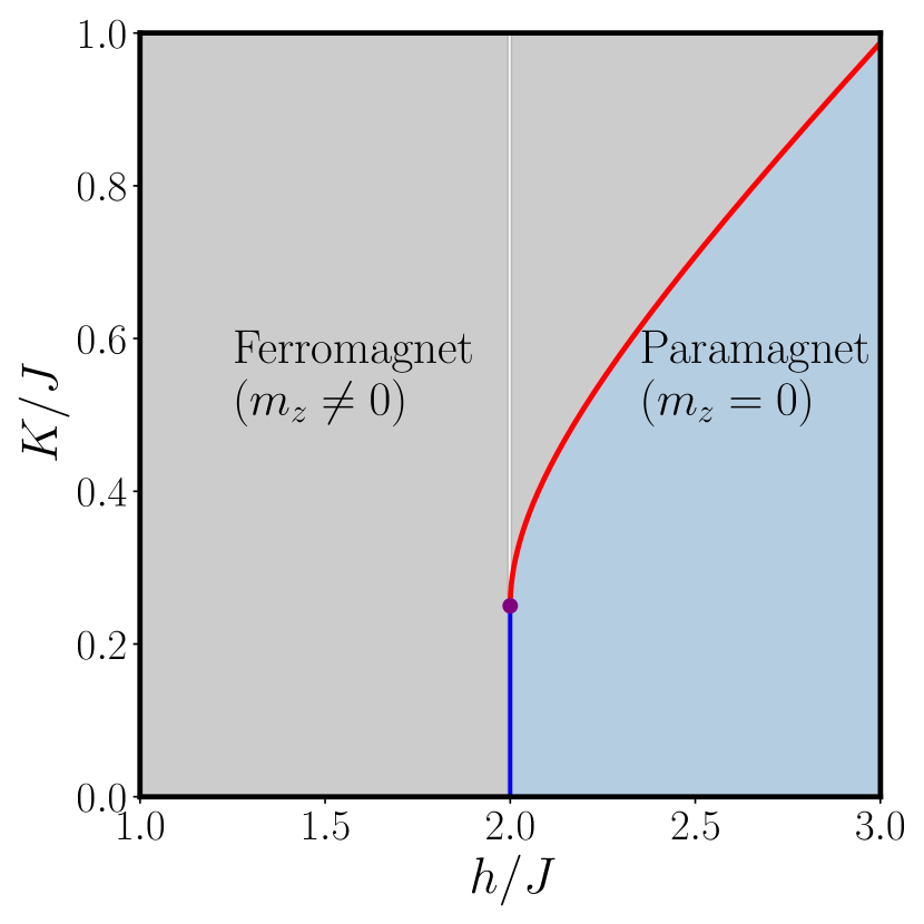
Figure 1: The ground-state ($T=0$) phase diagram of the model defined in Eq. (1) in the $(K/J,h/J)$ plane. It corresponds to both microcanonical and canonical ensembles. The phase-diagram displays a paramagnetic phase with $m_{z}=0$ (grey shaded area) in the high $K/J$ low $h/J$ region. This phase is separated from the ferromagnetic phase where $m_{z}$ is non vanishing (blue shaded area) by a second order transition line at $h/J=2$ for $K/J<1/4$ (blue line). The transition becomes first-order (red line) at the tricritical point $(K/J=1/4,h/J=2$). The first-order line is given in Eq.  (18).

Phase-diagram in the canonical ensemble: Let us consider the free energy of the model

$$f(\beta,J,h,K)=e-{\cal S}/\beta=-Js^{2}m_{z}^{2}-Ks^{4}m_{z}^{4}$$

$$-hs\sqrt{1-m_{z}^{2}}+\frac{1}{\beta}\left[\frac{1+s}{2}\ln\frac{1+s}{2}+\frac{1-s}{2}\ln\frac{1-s}{2}\right]\leavevmode\nobreak\ .$$ (19)

In order to find the equilibrium state of the system, one needs to minimize $f$ with respect to $s$ and $m$. Minimizing (Ensemble inequivalence in long-range quantum systems) with respect to $s$ first, we obtain an expansion of $s$ as a function of $m_{z}$,

$$s=s_{0}+am_{z}^{2}+O(m_{z}^{4})$$ (20)

where

$$s_{0} =\tanh(\beta h)\leavevmode\nobreak\ ,$$ (21a)

$$a =\beta(1-s_{0}^{2})(2Js_{0}-\frac{h}{2})\leavevmode\nobreak\ .$$ (21b)

Inserting the expansion (20) in the free energy (Ensemble inequivalence in long-range quantum systems), one obtains an expansion of $f$ in powers of $m_{z}^{2}$:

$$f=f_{0}+b_{2}m_{z}^{2}+b_{4}m_{z}^{4}+O(m_{z}^{6})\leavevmode\nobreak\ ,$$ (22)

with

$$f_{0} =-hs_{0}+\frac{1}{\beta}{\cal S}(s_{0})\leavevmode\nobreak\ ,$$ (23a)

$$b_{2} =\frac{1}{2}hs_{0}-Js_{0}^{2}\leavevmode\nobreak\ .$$ (23b)

At criticality $b_{2}=0$, yielding

$$s_{0}=\frac{h}{2J}\leavevmode\nobreak\ ,$$ (24)

and the critical line is given by

$$\frac{h}{2J}=\tanh{\beta h}\leavevmode\nobreak\ ,$$ (25)

as long as $b_{4}>0$. At low temperature the critical line is given, to leading order, by

$$\frac{h}{2J}\approx 1-2e^{-2\beta h}\leavevmode\nobreak\ .$$ (26)

To proceed, we evaluate $b_{4}$ and locate the tricritical point at $b_{2}=b_{4}=0$. We first expand the entropy in powers $\delta s$ for $s=s_{0}+\delta s$,

$${\cal S}(s)\approx{\cal S}(s_{0})+\frac{1}{2\beta}\ln\left(\frac{1+s_{0}}{1-s_{0}}\right)\delta s+\frac{1}{2\beta}\ln\left(\frac{1}{1-s_{0}^{2}}\right)\delta s^{2}.$$ (27)

Using this expansion with $\delta s=am_{z}^{2}$, one finds that on the critical line $b_{2}=0$ the expression for $b_{4}$ is

$$b_{4}=-(2Js_{0}-\frac{1}{2}h)a-(Ks_{0}^{4}-\frac{1}{8}hs_{0})+\frac{1}{2\beta}\frac{1}{1-s_{0}^{2}}a^{2}\leavevmode\nobreak\ .$$ (28)

Note that, due the fact that $\partial f/\partial s|_{s_{0}}=0$, higher order terms in the expansion (20) of $s$ do not contribute to $b_{4}$. Using (21b) for $a$, we obtain

$$b_{4}=-(Ks_{0}^{4}-\frac{h}{8}s_{0})-\frac{1}{8}\beta h^{2}(1-s_{0}^{2})\leavevmode\nobreak\ ,$$ (29)

where at low temperature

$$s_{0}=1-2e^{-2\beta h}\leavevmode\nobreak\ .$$ (30)

We finally arrive at the following expressions for the critical line ($b_{2}=0$) and the tricritical point ($b_{2}=b_{4}=0$) in the canonical ensemble ([CE])

$$b_{2}=0:\,\,\,\,h_{c}[CE]=2J(1-2e^{-4\beta J})\leavevmode\nobreak\ ,$$ (31)

$$b_{4}=0:\,\,\,\,K_{tcp}[CE]=\frac{J}{4}-2\beta J^{2}e^{-4\beta J}\leavevmode\nobreak\ .$$ (32)

Phase-diagram in the microcanonical ensemble: The microcanonical phase-diagram can be readily obtained by minimizing the energy at constant entropy. The energy is given by

$$\varepsilon=-Js^{2}m_{z}^{2}-Ks^{4}m_{z}^{4}-hs\sqrt{1-m_{z}^{2}}$$

$$\approx-hs+\left(\frac{1}{2}hs-Js^{2}\right)m_{z}^{2}+\left(\frac{1}{8}hs-Ks^{4}\right)m_{z}^{4}+O(m_{z}^{6})\leavevmode\nobreak\ .$$ (33)

The entropy ${\cal S}(s)$ (14) is a function of $s$ only and thus one has to minimize the energy $\varepsilon$ with respect to $m_{z}$ at fixed $s$. The resulting critical line is

$$\frac{1}{2}hs-Js^{2}=0\leavevmode\nobreak\ ,$$ (34)

which, together with

$$\frac{1}{8}hs-Ks^{4}=0\leavevmode\nobreak\ ,$$ (35)

yields the tricritical point. To proceed, one has to express $s$ in terms of the temperature. On the critical line, where $m_{z}=0$, the energy is given by $\varepsilon=-hs$. Thus,

$$\beta=\frac{\partial{\cal S}}{\partial\varepsilon}=-\frac{1}{h}\frac{\partial{\cal S}}{\partial s}=\frac{1}{2h}\ln\frac{1-s}{1+s}\leavevmode\nobreak\ ,$$ (36)

which gives

$$s=\tanh{\beta h}\approx 1-2e^{-2\beta h}\leavevmode\nobreak\ .$$ (37)

Inserting expression (37) in (34), the microcanonical ([MCE]) critical line becomes

$$h_{c}[MCE]=2J\left(1-2e^{-4\beta J}\right)\leavevmode\nobreak\ .$$ (38)

On the critical line, Eq. (35) becomes $J=4Ks^{2}$, which yields the tricritical point at

$$K_{tcp}[MCE]=J\left(\frac{1}{4}+e^{-4\beta J}\right)\leavevmode\nobreak\ .$$ (39)

When compared with the canonical analysis, this result presents an example of ensemble inequivalence. While the two ensembles lead to the same expression for the critical lines, (31), (38), they display distinct tricritical points. At a given temperature, the canonical tricritical point (32) is located at a lower value of $K/J$ than the microcanonical one (39), (see Fig.2 for the $(h/J,K/J)$ phase-diagram at a given low temperature).

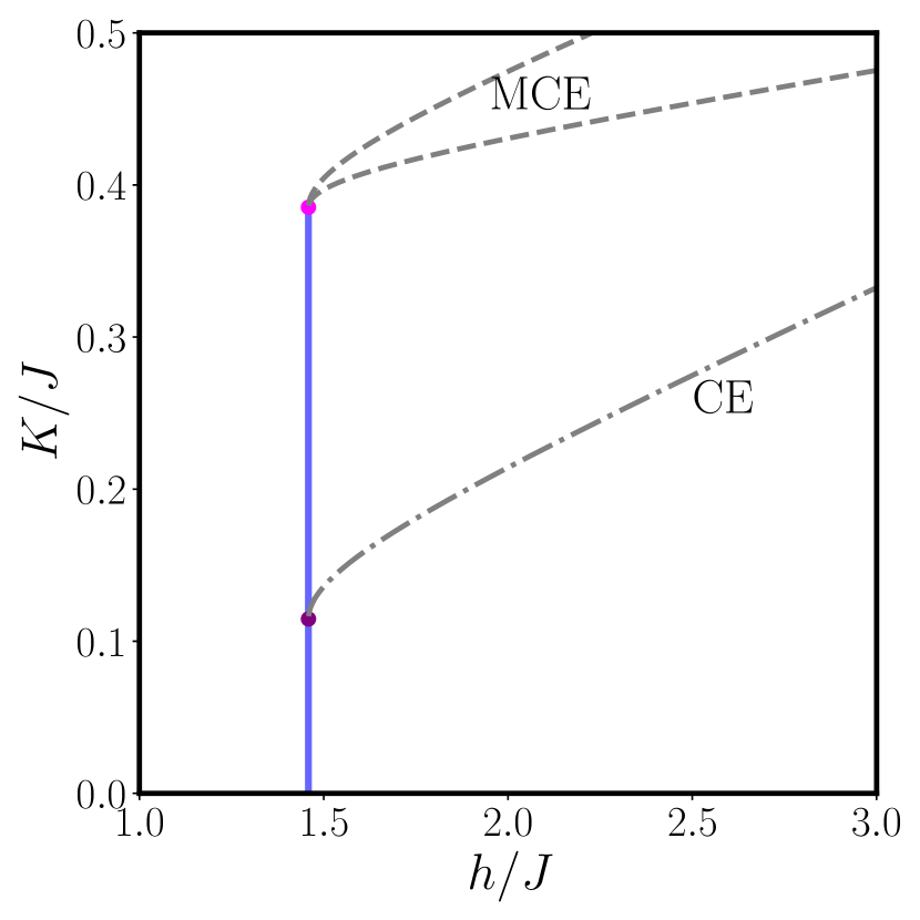
Figure 2: The canonical and microcanonical $(h/J,K/J)$ phase-diagrams at a given temperature ($\beta J=1/2$). The microcanonical critical line coincides with the canonical one, but extends beyond the canonical tricritical point. While the critical line (blue) is drawn in scale, the first order lines (gray dashed lines in the microcanonical ensemble and a gray dot-dashed line in the canonical one) are only drawn schematically.

In Fig.3 we display the tricritical coupling $K/J$ in the two ensembles, (32) and (39), as a function of $T/J$ at low temperatures. While the tricritical points coincide at $T=0$, the microcanonical one changes slower with temperature. Note that at any given temperature the magnetic field $h/J$ at the tricritical point is the same in the two ensembles.

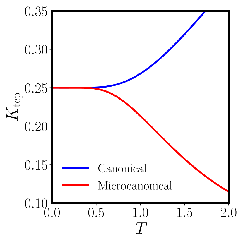
Figure 3: The position of the trictitical point $K/J$ against $T/J$ in the canonical and microcanonical ensembles.

Conclusions: In this paper we studied the phase-diagram of a model with long-range and multi-spin interactions, which is known to exhibit a paramagnetic to ferromagnetic quantum phase-transition at zero temperature. This transition has first-order and second-order branches separated by a tricritical point. We studied the model at finite temperature, where we have shown that the model exhibits different phase-diagrams when analyzed in the canonical and the microcanonical ensembles. We found that, although the two ensembles yield the same phase-diagram at $T=0$, the two phase-diagrams differ from each other at finite temperature. In particular, we found that the position of the tricritical point is not the same in the two ensembles. In the canonical ensemble the finite temperature correction to the position of the tricritical point is larger than in the microcanonical ensemble. It would be interesting to explore the general validity of these result by studying other quantum models with long-range interactions, particularly in models with power-law decaying interactions.

As AMO techniques continue to advance, we expect that our results could be experimentally tested on quantum platforms, particularly in the context of cold atoms within cavity setups. Indeed, while the Hamiltonian in Eq. (11) with $K=0$ has already been employed in the description of cavity QED platforms [34, 65, 66], the realization of the four body term at $K>0$ may be achieved by exploiting recent finding on cavity-mediated pair creation [67].

Acknowledgments: Valuable discussions with G. Gori and A. Trombettoni are gratefully acknowledged. Relevant discussion on the experimental feasibility of our research with T. Donner are also acknowledged. This work is supported by the Deutsche Forschungsgemeinschaft (DFG, German Research Foundation) under Germany’s Excellence Strategy EXC2181/1-390900948 (the Heidelberg STRUCTURES Excellence Cluster). This work is part of MUR-PRIN2017 project “Coarse-grained description for non-equilibrium systems and transport phenomena (CONEST)” No. 201798CZL whose partial financial support is acknowledged. DM acknowledges the support of the Center for Scientific Excellence of the Weizmann Institute of Science. This research was supported in part by grants NSF PHY-1748958 and PHY-2309135 to the Kavli Institute for Theoretical Physics (KITP).

References

- Lukin [2003] M. D. Lukin, Colloquium: Trapping and manipulating photon states in atomic ensembles, Rev. Mod. Phys. 75, 457 (2003).
- Saffman et al. [2010] M. Saffman, T. G. Walker, and K. Mølmer, Quantum information with Rydberg atoms, Rev. Mod. Phys. 82, 2313 (2010).
- Britton et al. [2012] J. W. Britton, B. C. Sawyer, A. C. Keith, C. C. J. Wang, J. K. Freericks, H. Uys, M. J. Biercuk, and J. J. Bollinger, Engineered two-dimensional Ising interactions in a trapped-ion quantum simulator with hundreds of spins, Nature 484, 489 (2012).
- Bloch et al. [2008] I. Bloch, J. Dalibard, and W. Zwerger, Many-body physics with ultracold gases, Reviews of Modern Physics 80, 885 (2008).
- Blatt and Roos [2012] R. Blatt and C. F. Roos, Quantum simulations with trapped ions, Nat. Phys. 8, 277 (2012).
- Monroe et al. [2021] C. Monroe, W. C. Campbell, L.-M. Duan, Z.-X. Gong, A. V. Gorshkov, P. W. Hess, R. Islam, K. Kim, N. M. Linke, G. Pagano, P. Richerme, C. Senko, and N. Y. Yao, Programmable quantum simulations of spin systems with trapped ions, Rev. Mod. Phys. 93, 025001 (2021).
- Mivehvar et al. [2021] F. Mivehvar, F. Piazza, T. Donner, and H. Ritsch, Cavity qed with quantum gases: new paradigms in many-body physics, Advances in Physics 70, 1–153 (2021).
- Defenu et al. [2023] N. Defenu, T. Donner, T. Macrì, G. Pagano, S. Ruffo, and A. Trombettoni, Long-range interacting quantum systems, Rev. Mod. Phys. 95, 035002 (2023).
- Angelini et al. [2014] M. C. Angelini, G. Parisi, and F. Ricci-Tersenghi, Relations between short-range and long-range ising models, Phys. Rev. E 89, 062120 (2014).
- Defenu et al. [2015] N. Defenu, A. Trombettoni, and A. Codello, Fixed-point structure and effective fractional dimensionality for O( N) models with long-range interactions, Phys. Rev. E 92, 289 (2015).
- Defenu et al. [2016] N. Defenu, A. Trombettoni, and S. Ruffo, Anisotropic long-range spin systems, Phys. Rev. B 94, 224411 (2016).
- Defenu et al. [2017] N. Defenu, A. Trombettoni, and S. Ruffo, Criticality and phase diagram of quantum long-range O( N) models, Phys. Rev. B 96, 1 (2017).
- Defenu et al. [2020] N. Defenu, A. Codello, S. Ruffo, and A. Trombettoni, Criticality of spin systems with weak long-range interactions, Journal of Physics A Mathematical General 53, 143001 (2020).
- Dauxois et al. [2002] T. Dauxois, V. Latora, A. Rapisarda, S. Ruffo, and A. Torcini, Dynamics and Thermodynamics of Systems with Long-Range Interactions, edited by T. Dauxois, S. Ruffo, E. Arimondo, and M. Wilkens (Springer Berlin Heidelberg, Berlin, Heidelberg, 2002) pp. 458–487.
- Campa et al. [2009] A. Campa, T. Dauxois, and S. Ruffo, Statistical mechanics and dynamics of solvable models with long-range interactions, Phys. Rep. 480, 57 (2009).
- Campa et al. [2014] A. Campa, T. Dauxois, D. Fanelli, and S. Ruffo, Physics of Long-Range Interacting Systems (Oxford Univ. Press, 2014).
- Levin et al. [2014] Y. Levin, R. Pakter, F. B. Rizzato, T. N. Teles, and F. P. Benetti, Nonequilibrium statistical mechanics of systems with long-range interactions, Physics Reports 535, 1 (2014).
- Barré et al. [2001] J. Barré, D. Mukamel, and S. Ruffo, Inequivalence of ensembles in a system with long-range interactions, Phys. Rev. Lett. 87, 030601 (2001).
- Kastner [2011] M. Kastner, Diverging Equilibration Times in Long-Range Quantum Spin Models, Phys. Rev. Lett. 106, 130601 (2011).
- Schütz and Morigi [2014] S. Schütz and G. Morigi, Prethermalization of atoms due to photon-mediated long-range interactions, Phys. Rev. Lett. 113, 203002 (2014).
- Schütz et al. [2016] S. Schütz, S. B. Jäger, and G. Morigi, Dissipation-Assisted Prethermalization in Long-Range Interacting Atomic Ensembles, Phys. Rev. Lett. 117, 083001 (2016).
- Defenu [2021] N. Defenu, Metastability and discrete spectrum of long-range systems, Proc. Nat. Acad. Sci. , In press (2021).
- Mukamel et al. [2005] D. Mukamel, S. Ruffo, and N. Schreiber, Breaking of ergodicity and long relaxation times in systems with long-range interactions, Phys. Rev. Lett. 95, 240604 (2005).
- Borgonovi et al. [2004] F. Borgonovi, G. L. Celardo, M. Maianti, and E. Pedersoli, Broken ergodicity in classically chaotic spin systems, Journal of Statistical Physics 116, 1435 (2004).
- Kastner [2010a] M. Kastner, Nonequivalence of Ensembles for Long-Range Quantum Spin Systems in Optical Lattices, Phys. Rev. Lett. 104, 240403 (2010a).
- Kastner [2010b] M. Kastner, Nonequivalence of ensembles in the curie–weiss anisotropic quantum heisenberg model, J. Stat. Phys. 2010, P07006 (2010b).
- Del Re et al. [2016] L. Del Re, M. Fabrizio, and E. Tosatti, Nonequilibrium and nonhomogeneous phenomena around a first-order quantum phase transition, Phys. Rev. B 93, 125131 (2016).
- Petrov [2014] D. S. Petrov, Elastic multibody interactions on a lattice, Phys. Rev. A 90, 021601 (2014).
- Goban et al. [2018] A. Goban, R. B. Hutson, G. E. Marti, S. L. Campbell, M. A. Perlin, P. S. Julienne, J. P. D’Incao, A. M. Rey, and J. Ye, Emergence of multi-body interactions in a fermionic lattice clock, Nature (London) 563, 369 (2018).
- Zwerger [2019] W. Zwerger, Quantum-unbinding near a zero temperature liquid–gas transition, Journal of Statistical Mechanics: Theory and Experiment 2019, 103104 (2019).
- Griesmaier et al. [2005] A. Griesmaier, J. Werner, S. Hensler, J. Stuhler, and T. Pfau, Bose-einstein condensation of chromium, Phys. Rev. Lett. 94, 160401 (2005).
- Micheli et al. [2006] A. Micheli, G. K. Brennen, and P. Zoller, A toolbox for lattice-spin models with polar molecules, Nat. Phys. 2, 341 (2006).
- Ni et al. [2008] K.-K. Ni, S. Ospelkaus, M. H. G. de Miranda, A. Pe’er, B. Neyenhuis, J. J. Zirbel, S. Kotochigova, P. S. Julienne, D. S. Jin, and J. Ye, A high phase-space-density gas of polar molecules, Science 322, 231 (2008).
- Morrison and Parkins [2008a] S. Morrison and A. S. Parkins, Dynamical quantum phase transitions in the dissipative Lipkin-Meshkov-Glick model with proposed realization in optical cavity QED, Phys. Rev. Lett. 100, 040403 (2008a).
- Larson [2010] J. Larson, Circuit qed scheme for the realization of the lipkin-meshkov-glick model, EPL (Europhysics Letters) 90, 54001 (2010).
- Wu et al. [2023] Z. Wu, J. Fan, X. Zhang, J. Qi, and H. Wu, Signatures of prethermalization in a quenched cavity-mediated long-range interacting fermi gas, Phys. Rev. Lett. 131, 243401 (2023).
- Albash and Lidar [2018] T. Albash and D. A. Lidar, Adiabatic quantum computation, Rev. Mod. Phys. 90, 015002 (2018).
- Lipkin et al. [1965] H. J. Lipkin, N. Meshkov, and A. J. Glick, Validity of many-body approximation methods for a solvable model, Nuclear Physics 62, 188 (1965).
- Meshkov et al. [1965] N. Meshkov, A. J. Glick, and H. J. Lipkin, Validity of many-body approximation methods for a solvable model. (II). Linearization procedures, Nuclear Physics 62, 199 (1965).
- Glick et al. [1965] A. J. Glick, H. J. Lipkin, and N. Meshkov, Validity of many-body approximation methods for a solvable model. (III). Diagram summations, Nuclear Physics 62, 211 (1965).
- Dicke [1954] R. H. Dicke, Coherence in spontaneous radiation processes, Phys. Rev. 93, 99 (1954).
- Baumann et al. [2010] K. Baumann, C. Guerlin, F. Brennecke, and T. Esslinger, Dicke quantum phase transition with a superfluid gas in an optical cavity, Nature 464, 1301 (2010).
- Landig et al. [2015] R. Landig, F. Brennecke, R. Mottl, T. Donner, and T. Esslinger, Measuring the dynamic structure factor of a quantum gas undergoing a structural phase transition, Nat. Comm. 6, 7046 (2015).
- Reslen et al. [2005] J. Reslen, L. Quiroga, and N. F. Johnson, Direct equivalence between quantum phase transition phenomena in radiation-matter and magnetic systems: Scaling of entanglement, EPL 69, 8 (2005).
- Schütz et al. [2015] S. Schütz, S. B. Jäger, and G. Morigi, Thermodynamics and dynamics of atomic self-organization in an optical cavity, Phys. Rev. A 92, 063808 (2015).
- Leroux et al. [2010] I. D. Leroux, M. H. Schleier-Smith, and V. Vuletić, Implementation of cavity squeezing of a collective atomic spin, Phys. Rev. Lett. 104, 073602 (2010).
- Bentsen et al. [2019] G. Bentsen, I.-D. Potirniche, V. B. Bulchandani, T. Scaffidi, X. Cao, X.-L. Qi, M. Schleier-Smith, and E. Altman, Integrable and chaotic dynamics of spins coupled to an optical cavity, Phys. Rev. X 9, 041011 (2019).
- Davis et al. [2019] E. J. Davis, G. Bentsen, L. Homeier, T. Li, and M. H. Schleier-Smith, Photon-mediated spin-exchange dynamics of spin-1 atoms, Phys. Rev. Lett. 122, 010405 (2019).
- Davis et al. [2020] E. J. Davis, A. Periwal, E. S. Cooper, G. Bentsen, S. J. Evered, K. Van Kirk, and M. H. Schleier-Smith, Protecting spin coherence in a tunable heisenberg model, Phys. Rev. Lett. 125, 060402 (2020).
- Gallemí et al. [2016] A. Gallemí, G. Queraltó, M. Guilleumas, R. Mayol, and A. Sanpera, Quantum spin models with mesoscopic bose-einstein condensates, Phys. Rev. A 94, 063626 (2016).
- Ho [1998] T.-L. Ho, Spinor bose condensates in optical traps, Phys. Rev. Lett. 81, 742 (1998).
- Stenger et al. [1998] J. Stenger, S. Inouye, D. M. Stamper-Kurn, H. J. Miesner, A. P. Chikkatur, and W. Ketterle, Spin domains in ground-state Bose-Einstein condensates, Nature (London) 396, 345 (1998).
- Chang et al. [2004] M.-S. Chang, C. D. Hamley, M. D. Barrett, J. A. Sauer, K. M. Fortier, W. Zhang, L. You, and M. S. Chapman, Observation of spinor dynamics in optically trapped bose-einstein condensates, Phys. Rev. Lett. 92, 140403 (2004).
- Schmaljohann et al. [2004] H. Schmaljohann, M. Erhard, J. Kronjäger, M. Kottke, S. van Staa, L. Cacciapuoti, J. J. Arlt, K. Bongs, and K. Sengstock, Dynamics of spinor bose-einstein condensates, Phys. Rev. Lett. 92, 040402 (2004).
- Hoang et al. [2016] T. M. Hoang, M. Anquez, B. A. Robbins, X. Y. Yang, B. J. Land, C. D. Hamley, and M. S. Chapman, Parametric excitation and squeezing in a many-body spinor condensate, Nature Communications 7, 11233 (2016).
- Weimer et al. [2010] H. Weimer, M. Müller, I. Lesanovsky, P. Zoller, and H. P. Büchler, A rydberg quantum simulator, Nature Physics 6, 382 (2010).
- Henkel et al. [2010] N. Henkel, R. Nath, and T. Pohl, Three-dimensional roton excitations and supersolid formation in rydberg-excited bose-einstein condensates, Phys. Rev. Lett. 104, 195302 (2010).
- Gil et al. [2014] L. I. R. Gil, R. Mukherjee, E. M. Bridge, M. P. A. Jones, and T. Pohl, Spin squeezing in a rydberg lattice clock, Phys. Rev. Lett. 112, 103601 (2014).
- Zeiher et al. [2015] J. Zeiher, P. Schauß, S. Hild, T. Macrì, I. Bloch, and C. Gross, Microscopic characterization of scalable coherent rydberg superatoms, Phys. Rev. X 5, 031015 (2015).
- Jau et al. [2016] Y. Y. Jau, A. M. Hankin, T. Keating, I. H. Deutsch, and G. W. Biedermann, Entangling atomic spins with a rydberg-dressed spin-flip blockade, Nature Physics 12, 71 (2016).
- Will et al. [2010] S. Will, T. Best, U. Schneider, L. Hackermüller, D.-S. Lühmann, and I. Bloch, Time-resolved observation of coherent multi-body interactions in quantum phase revivals, Nature 465, 197 (2010).
- Büchler et al. [2007] H. P. Büchler, A. Micheli, and P. Zoller, Three-body interactions with cold polar molecules, Nat. Phys. 3, 726 (2007).
- Lieb [1973] E. H. Lieb, The classical limit of quantum spin systems, Commun. Math. Phys 31, 327 (1973).
- Granet [2023] E. Granet, Exact mean-field solution of a spin chain with short-range and long-range interactions, SciPost Phys. 14, 133 (2023).
- Morrison and Parkins [2008b] S. Morrison and A. S. Parkins, Collective spin systems in dispersive optical cavity qed: Quantum phase transitions and entanglement, Phys. Rev. A 77, 043810 (2008b).
- Cosme et al. [2023] J. G. Cosme, J. Skulte, and L. Mathey, Bridging closed and dissipative discrete time crystals in spin systems with infinite-range interactions, Phys. Rev. B 108, 024302 (2023).
- Finger et al. [2023] F. Finger, R. Rosa-Medina, N. Reiter, P. Christodoulou, T. Donner, and T. Esslinger, Spin- and momentum-correlated atom pairs mediated by photon exchange and seeded by vacuum fluctuations, arXiv 2303.11326 (2023).