The energy spectrum of a quantum vortex loop
moving in a long pipe

S.V. Talalov

Dept. of Applied Mathematics, Togliatti State University,
14 Belorusskaya str., Tolyatti, 445020 Russia.
svt_19@mail.ru

Abstract

In this study we consider the closed vortex filament that moves in a pipe of length $L>>R_{1}$, where $R_{1}$ means inner radius of the pipe. The vortex filament is described in the Local Induction Approximation. We quantize this dynamical system and calculate the spectrum both circulation and energy. In the study, we focus on the case $L\to\infty$.

keywords: local induction approximation; vortex filament quantization; extended Galilei group.

1 Introduction

 

Usually, quantization of a complex dynamical system is an ambiguous procedure. The development of quantum theory really confirms Dirac’s famous words: ”…methods of quantization are all of the nature of practical rules, whose application depends on consideration of simplicity” [1]. For instance, the quantization of canonically equivalent but different sets of classical variables can lead to physically different results at the quantum level. This is true even for simple systems from a text-book: so, the quantization of a harmonic oscillator in terms of action-angle variables demonstrates many unexpected and interesting results [2]. As a rule, the problem arises when we quantize a complex dynamic system, especially in the cases where experiments cannot confirm or disprove the final results for the spectrum of observable values.

Our study is devoted to the quantum description of the perturbed vortex ring of radius $R$. This ring (vortex filament) moves in the domain $D\subset{\sf R}_{3}$ that is defined by the conditions

$$\rho~{}\leq~{}R_{1}\,,\qquad-\frac{L}{2}~{}<~{}z~{}<~{}\frac{L}{2},\qquad\qquad R_{1}<<L\,,\quad R<R_{1}\,.$$ (1)

Cylindrical coordinate system $(\rho,\varphi,z)$ with corresponding basis $(\,\boldsymbol{n}_{\rho}\,,\boldsymbol{n}_{\varphi}\,,\boldsymbol{n}_{z}\,)$ is associated with domain (1) naturally; the $z$ axis ($\boldsymbol{n}_{z}$) is directed along the pipe. In fact, we will consider the asymptotic case $L\to\infty$, taking into account that the value $L<\infty$ in reality. Of course, the theory of quantum vortices has been around for decades. A lot of articles are devoted to this issue. Here we note only some fundamental books of [3, 4, 5] that reflect different periods of research and approaches to the problem.

For our further studies, we use a representation for smooth closed filament of length $S$ in the form

$${\boldsymbol{r}}(\tau,\xi)~{}=~{}{\boldsymbol{q}}+{R}\int\limits_{0}^{2\pi}\left[\,{\xi-\eta}\,\right]{\boldsymbol{j}}(\tau,\eta)d\eta\,,\qquad R=\frac{S}{2\pi}\,,\qquad\xi=\frac{s}{R}\,,$$ (2)

where parameter $\tau$ describes the curve evolution. Vector ${\boldsymbol{q}}={\boldsymbol{q}}(\tau)$ defines the position of the filament (for example, the center of the circular vortex ring) in some coordinate system. The notation $[\,x\,]$ means the integer part of the number $x/{2\pi}$:

$$[\,0\,]=0\,,\qquad[\,x+2\pi\,]=[\,x\,]+1\,,\qquad\forall\,x\,.$$ (3)

Vector ${\boldsymbol{j}}(\tau,\eta)$ is the unit tangent (affine) vector for this filament. Let the vector ${\boldsymbol{r}}(\tau,\xi)$ satisfies the Local Induction Equation (LIE, see [6] for example):

$$\partial_{\tau}{\boldsymbol{r}}(\tau,\xi)~{}=~{}\frac{\alpha}{R}\,\partial_{\xi}{\boldsymbol{r}}(\tau,\xi)\times\partial_{\xi}^{\,2}{\boldsymbol{r}}(\tau,\xi)\,.$$ (4)

Evolution parameter $\tau$ was defined here as $\tau={t\Gamma}/{4\pi R^{2}}$, where $t$ is real time and symbol $\Gamma$ means the circulation. Let’s note that we have redefined the evolution parameter for the curve (2) only. Any physical quantity (for example, circulation $\Gamma$) that is not associated directly with curve (2) as a geometric object, remains unchanged. Dimensionless parameter $\alpha$ depends on the filament core radius $a<<R$ as well as some details of regularization procedure that has been fulfilled to deduce equation (4) (see, for example, [6, 7]). In the future, we will exclude this parameter from consideration by redefining of the parameter $\tau$: $\tau\to\alpha\tau$ Then, the function ${\boldsymbol{j}}(\tau,\eta)$ satisfies the equation for continuous Heisenberg spin chain:

$$\partial_{\tau}{\boldsymbol{j}}(\tau,\xi)~{}=~{}{\boldsymbol{j}}(\tau,\xi)\times\partial_{\xi}^{\,2}{\boldsymbol{j}}(\tau,\xi)\,.$$ (5)

2 Classical dynamic system

 

We consider the small ($\varepsilon<<1$) perturbation ${\boldsymbol{j}}_{p}(\tau,\xi)$ of the vortex ring ${\boldsymbol{j}_{0}}(\xi)$:

$$\boldsymbol{j}(\tau,\xi)~{}=~{}{\boldsymbol{j}_{0}}(\xi)+\varepsilon{\boldsymbol{j}}_{p}(\tau,\xi)\,,\qquad\qquad{\boldsymbol{j}}_{p}(\tau,\xi+2\pi)={\boldsymbol{j}}_{p}(\tau,\xi)\,,$$ (6)

where unperturbed vector $\boldsymbol{j}_{0}(\xi)$ is a tangent vector for the circular filament:

$$\boldsymbol{j}_{0}(\xi)~{}=~{}\boldsymbol{e}_{\phi}\,.$$

The vectors $({\boldsymbol{e}_{\rho}}\,,\boldsymbol{e}_{\phi}\,,{\boldsymbol{e}_{z}}\,)$ denote the local cylindrical basis that is associated naturally with this circular filament. Please note that this basis differs from the basis $(\,\boldsymbol{n}_{\rho}\,,\boldsymbol{n}_{\varphi}\,,\boldsymbol{n}_{z}\,)$ which was previously associated with domain $D$.

Additionally, we suppose that the excitations (6) be transverse:

$${\boldsymbol{j}}_{p}(\tau,\xi){\boldsymbol{j}_{0}}(\xi)~{}\equiv~{}0\,$$ (7)

The small perturbation of the circular vortex filament without the restriction (7) has been studied in the work [8]. Various aspects of the theory related to vortex ring oscillations have also been studied in the works [9, 10]. The small perturbations of straight vortex filaments were studied in the work [11].

Condition (7) leads to decomposition

$${\boldsymbol{j}}_{p}(\tau,\xi)~{}=~{}j_{\rho}(\tau,\xi){\boldsymbol{e}}_{\rho}+j_{z}(\tau,\xi){\boldsymbol{e}_{z}}\,,$$ (8)

For convenience, we define the complex-valued function

$${\mathfrak{J}}(\tau,\xi)~{}=~{}j_{\rho}(\tau,\xi)+{\rm i}j_{z}(\tau,\xi)\,.$$

This function allows us define the complex amplitudes ${\mathfrak{j}}_{\,n}(\tau)$:

$${\mathfrak{J}}(\tau,\xi)~{}=~{}\sum_{n}{\mathfrak{j}}_{\,n}(\tau)\,e^{\,i\,\,n\xi}\,.$$ (9)

Taking into account the terms of the order $\varepsilon$ only, we can deduce that amplitude ${\mathfrak{J}}(\tau,\xi)$ satisfies the linear equation [12]

$$\partial_{\tau}{\mathfrak{J}}=-i\partial_{\xi}^{\,2}{\mathfrak{J}}-\frac{i}{2}\Bigl{(}{\mathfrak{J}}-\overline{\,{\mathfrak{J}}\,}\,\Bigr{)}\,.$$ (10)

Consequently,

$${\mathfrak{J}}(\tau,\xi)~{}=~{}\sum_{n}{\mathfrak{j}}_{\,n}\,e^{\,i\,[\,n\,\xi+n\sqrt{n^{2}-1}\,\tau\,]}\,,$$ (11)

where the amplitudes ${\mathfrak{j}}_{\,n}$ satisfy the condition  $\overline{\,{\mathfrak{j}}\,}_{\,-n}~{}=~{}2\left[n\sqrt{n^{2}-1}-n^{2}+{1}/{2}\right]{\mathfrak{j}}_{\,n}\,.$ Thus, we can declare the vector $\boldsymbol{q}$ and amplitudes ${\mathfrak{j}}\,_{\,-n}$, where $n=0,1,2,\dots$, as independent variables. These variables describe the dynamics of small-perturbed circle-like curve ${\boldsymbol{r}}(\tau,\xi)$ in accordance with Eq.(4). Note that we still describe the evolution of curve (2) as a formal geometric object only. According to our assumption, the curve ${\boldsymbol{r}}(\tau,\xi)$, is a vortex filament. However, variables $\boldsymbol{q}$ and ${\mathfrak{j}}\,_{\,-n}$ do not take into account the movement of the surrounding fluid any way. That is why we include the circulation $\Gamma$ as an additional independent variable in our theory. Therefore, we describe the dynamics of a filament by the following set ${\cal A}$ of the independent variables:

$${\cal A}~{}=~{}\{\,\Gamma\,,\boldsymbol{q}\,,\boldsymbol{j}(\xi)\,\}\,.$$

Although these variables take into account the movement of the surrounding fluid in a minimal way, they are inconvenient for subsequent quantization. Therefore, we replace the set ${\cal A}$ by the set ${\cal A}^{\prime}$, where

$${\cal A}~{}\subset~{}{\cal A}^{\,\prime}~{}=~{}\bigl{\{}\,{\boldsymbol{p}}\,,{\boldsymbol{q}}\,;{\boldsymbol{j}}(\xi)\,\bigr{\}}\,.$$ (12)

Inclusion ${\cal A}~{}\subset~{}{\cal A}^{\,\prime}$ is performed by means of a well-known hydrodynamic formula

$${\boldsymbol{p}}~{}=~{}\frac{\varrho_{0}}{2}\,\int\,\boldsymbol{r}\times\boldsymbol{w}(\boldsymbol{r})\,dV\,,$$ (13)

where constant $\varrho_{0}$ means a fluid density and vector-function $\boldsymbol{w}(\boldsymbol{r})$ means the vorticity of the vortex filament. This function is calculated as

$${\boldsymbol{w}}(\boldsymbol{r})~{}=~{}\Gamma\int\limits_{0}^{2\pi}\,\hat{\delta}(\boldsymbol{r}-\boldsymbol{r}(\xi))\partial_{\xi}{\boldsymbol{r}}(\xi)d\xi\,.$$ (14)

Compact form for the formulas (13) and (14) is more convenient. Taking into account Eq.(2), we can write:

$${\boldsymbol{p}}~{}=~{}\varrho_{0}{R}^{2}\Gamma{\boldsymbol{f}}\,,\qquad{\boldsymbol{f}}~{}=~{}\frac{1}{2}\iint\limits_{0}^{2\pi}\left[\,{\xi-\eta}\,\right]\,{\boldsymbol{j}}(\eta)\times{\boldsymbol{j}}(\xi)d\xi d\eta\,.$$ (15)

It is clear that the replacement $\Gamma\to{\boldsymbol{p}}$ leads to the certain constraints on the set ${\cal A}^{\,\prime}$ in general. This issue has been investigated in the article [12] in detail. For our subsequent purposes, we assume ${\mathfrak{j}}\,_{\,0}=0$, just as ${\mathfrak{j}}\,_{\,-1}=0$ (see Eq. (11)). The last assumption makes independent momentum variations $\delta{\boldsymbol{p}}$ and small variations ${\boldsymbol{j}}_{p}$: so, the equality

$${\boldsymbol{p}}~{}=~{}\pi\varrho_{0}{R}^{2}\Gamma{\boldsymbol{e}}_{z}$$ (16)

is fulfilled in the case ${\mathfrak{j}}\,_{\,-1}=0$.

We are considering a non-relativistic theory; therefore, it is natural to declare the Galilei group ${\mathcal{G}}_{3}$ as the space-time symmetry group of our model. Moreover, we will consider the central extension $\widetilde{\mathcal{G}}_{3}$ of this group here. Corresponding central charge $m_{0}$ (this constant is interpreted as a ”mass”) completes the list of fundamental constants of the theory. The other constants are as follows: the fluid’s density $\varrho_{0}$, the speed of sound in this fluid $v_{0}$. In order to simplify some formulas, we will use the auxiliary constants $R_{0}=\sqrt[3\,]{m_{0}/\varrho_{0}}$, $~{}t_{0}=R_{0}/v_{0}$ and ${\cal E}_{0}=m_{0}v_{0}^{2}$ along with constants $\varrho_{0}$, $v_{0}$ and $m_{0}$.

The presence of the central extended Galilei group allows us to apply the group-theoretical approach to the definition of the energy of thin vortex filament. Indeed, the Lee algebra of the group $\widetilde{\mathcal{G}}_{3}$ has three Cazimir functions:

$${\hat{C}}_{1}=m_{0}{\hat{I}}\,,\quad{\hat{C}}_{2}=\left({\hat{M}}_{i}-\sum_{k,j=x,y,z}\epsilon_{ijk}{\hat{P}}_{j}{\hat{B}}_{k}\right)^{2}\quad{\hat{C}}_{3}=\hat{H}-\frac{1}{2m_{0}}\sum_{i=x,y,z}{\hat{P}}_{i}^{\,2}\,,$$

where ${\hat{I}}$ is the unit operator, ${\hat{M}}_{i}$, $\hat{H}$, ${\hat{P}}_{i}$ and ${\hat{B}}_{i}$ ($i=x,y,z$) are the respective generators of rotations, time and space translations and Galilean boosts. As it is well known, the function ${\hat{C}}_{3}$ can be interpreted as an ”internal energy of the particle”. In our model, the internal degrees of freedom are described by the function ${\mathfrak{J}}(\tau,\xi)$. This function is invariant under Galilei transformation; that is why ${\hat{C}}_{3}={\hat{C}}_{3}({\mathfrak{J}})$ in general. Let us postulate a formula for the Cazimir functions ${\hat{C}}_{3}$:

$${\hat{C}}_{3}~{}=~{}{\mathcal{E}}_{0}\sum_{n>1}|\,{\mathfrak{j}}_{\,-n}|^{2}n\sqrt{n^{2}-1}\,.$$

This formula will be justified after determining the Hamiltonian structure of the theory. Therefore, the following expression for the energy ${\mathcal{E}}$ is natural for our model:

$${\mathcal{E}}({\boldsymbol{p}}\,;{\mathfrak{j}}\,)=\frac{{\boldsymbol{p}}^{\,2}}{2m_{0}}+{\mathcal{E}}_{0}\sum_{n>1}|\,{\mathfrak{j}}_{\,-n}|^{2}n\sqrt{n^{2}-1}\,.$$ (17)

Let us define the Hamiltonian structure.

• The set ${\cal A}^{\,\prime}$ is interpreted as a phase space ${\mathcal{H}}$ quite naturally: ${\mathcal{H}}={\mathcal{H}}_{3}\times{\mathcal{H}}_{j}$. The space ${\mathcal{H}}_{3}$ is parametrized by the variables ${\boldsymbol{q}}$ and ${\boldsymbol{p}}$; this space is interpreted as a phase space of $3D$ free structureless particle. The phase space ${\mathcal{H}}_{j}$ is parametrized by the complex variables ${\mathfrak{j}}_{\,-n}$, $\overline{\,\mathfrak{j}}_{\,-n}$ ($n=0,1,\dots$).

• Poisson structure:

  $$\{p_{i}\,,q_{j}\} = \delta_{ij}\,,\qquad i,j=x,y,z\,,$$ (18)

  $$\{{\mathfrak{j}}_{\,m},\overline{\,\mathfrak{j}\,}_{\,n}\} = (i/{\mathcal{E}}_{0}t_{0})\,\delta_{mn}\,,\qquad m,n=-1,-2,\dots$$ (19)

  All other brackets vanish. The real variable ${\mathfrak{j}}_{\,0}$ annulates all brackets. Thus, the Poisson structure of the theory is degenerate in general: the value ${\mathfrak{j}}_{\,0}$ marks the symplectic sheets where the structure will be non-degenerate.

• Hamiltonian

  $$H({\boldsymbol{p}}\,;{\mathfrak{j}}\,)~{}=~{}{\mathcal{E}}({\boldsymbol{p}}\,;{\mathfrak{j}}\,)\,,$$ (20)

  where the function ${\mathcal{E}}({\boldsymbol{p}}\,;{\mathfrak{j}})$ was defined by the formula (17).

Hamiltonian (20) defines the evolution of the filament ${\boldsymbol{r}}(\xi)$ in ”conditional” time $t^{\#}=t_{0}\tau$. It is not difficult to make sure that the Hamiltonian (20) and the Poisson brackets (18), (19) generate dynamics

$${\boldsymbol{q}}(0) \longrightarrow {\boldsymbol{q}}(t^{\#})~{}=~{}{\boldsymbol{q}}(0)~{}+~{}\frac{\boldsymbol{p}}{m_{0}}\,t^{\#}\,,$$ (21)

$${\mathfrak{j}}_{-n}(0) \longrightarrow {\mathfrak{j}}_{-n}(t^{\#})~{}=~{}{\mathfrak{j}}_{-n}(0)\,e^{\,-i\,n\sqrt{n^{2}-1}\,(t^{\#}/t_{0})\,}$$

Among other things, these formulas demonstrate the fulfilled extension

$$\bigl{\{}\,{\boldsymbol{q}}\,;{\boldsymbol{j}}(\xi)\,\bigr{\}}~{}\longrightarrow~{}\bigl{\{}\,{\boldsymbol{p}}\,,{\boldsymbol{q}}\,;{\boldsymbol{j}}(\xi)\,\bigr{\}}\,$$

of the original dynamic system (4). Indeed, in accordance with Eq.(4)

$$\frac{d{\boldsymbol{q}}}{dt^{\#}}~{}=~{}\frac{R}{t_{0}}\,{\boldsymbol{e}}_{z}\,.$$

As opposed to Eq.(21), this formula corresponds to the following dependence ${\boldsymbol{q}}={\boldsymbol{q}}(t^{\#})$:

$${\boldsymbol{q}}(0)~{}\longrightarrow~{}{\boldsymbol{q}}(t^{\#})~{}=~{}{\boldsymbol{q}}(0)~{}+~{}{R}\,(t^{\#}/t_{0})\,{\boldsymbol{e}}_{z}\,.$$

3 Quantization and energy spectrum

 

Let’s quantize the constructed dynamic system. Firstly, we define a Hilbert space $\boldsymbol{H}$ of the quantum states. The structure of the phase space ${\mathcal{H}}$ makes the following construction natural:

$$\boldsymbol{H}=\boldsymbol{H}_{3}\otimes\boldsymbol{H}_{j}\,,$$ (22)

where the symbol $\boldsymbol{H}_{3}$ denotes the Hilbert space of a free structureless particle in the space ${\sf R}_{3}$ (the space $L^{2}({\sf R}_{3})$ in our case) and symbol $\boldsymbol{H}_{j}$ denotes the Fock space for the infinite number of the harmonic oscillators. This space is formed by the basic vectors

$$\bigl{(}\hat{a}^{+}(n_{1})\bigr{)}^{s_{1}}\dots\bigl{(}\hat{a}^{+}(n_{N})\bigr{)}^{s_{N}}|0\rangle\,,\qquad n_{i}\not=n_{j}\quad for\quad i\not=j\,,$$

where oscillators are numbered with numbers $n_{1},\dots,n_{N}$, $N=0,1,2,\dots$ and symbols $s_{j}$ denote corresponding occupation numbers. Creation and annihilation operators in the space $\boldsymbol{H}_{j}$ have standard commutation relations

$$[\,\hat{a}(m),\hat{a}^{+}(n)]=\delta_{mn}\hat{I}_{j}\,,\qquad\hat{a}(m)|\,0\rangle=0\,,\qquad m,n=1,2,\dots\,,\qquad|\,0\rangle\in\boldsymbol{H}_{j}\,,$$

where the operator $\hat{I}_{j}$ is unit operator in the space $\boldsymbol{H}_{j}$.

Our postulate of quantization is following:

$$\boldsymbol{q}~{}\to~{}\boldsymbol{q}\otimes\,\hat{I}_{j}\,,\qquad\boldsymbol{p}~{}\to~{}-i\hbar\nabla\otimes\,\hat{I}_{j}\,,\qquad{\mathfrak{j}}_{\,-n}~{}\to~{}\sqrt{\frac{\hbar}{t_{0}{\mathcal{E}}_{0}}}\,\Bigl{(}\hat{I}_{3}\otimes\,\hat{a}(n)\Bigr{)}\,,$$

where $n=1,2,\dots\,$. The unit operator $\hat{I}_{3}$ acts in the space $L^{2}({\sf R}_{3})$. In order to downsize the formulas, we will not write the constructions $(\dots\otimes\,\hat{I}_{j})$ and $(\hat{I}_{3}\otimes\,\dots)$ explicitly, hoping that this simplification will not lead to misunderstandings. As usual in a field theory, we postulate the normal ordering for the operators $\hat{a}(m)$ and $\hat{a}^{+}(n)$ when we quantize any products of the variables ${\mathfrak{j}}_{\,-n}$ and $\overline{\,{\mathfrak{j}}\,}_{\,-m}$. For example,

$$|{\mathfrak{j}}_{\,-n}|^{2}~{}\to~{}\frac{\hbar}{t_{0}{\mathcal{E}}_{0}}\hat{a}^{+}(n)\hat{a}(n)\,.$$

In this study we consider our system in the domain (1) only. Before calculating the energy spectrum, we quantize circulation $\Gamma$. Let’s pay attention that our approach allows us to find the spectrum of the value $\Gamma$ using conventional methods of quantum theory. Usually, the spectrum of this physical value is postulated, similar to the quantization rules in the old Bohr quantum mechanics. Arguments in favor of generalizing the standard expression for quantum circulation were discussed in more detail in the author’s article [13].

Squaring the Eq. (16), we have $SO(3)$ - invariant expression

$$\boldsymbol{p}^{2}~{}-~{}\pi^{2}\varrho_{0}^{2}R^{4}\Gamma^{2}~{}=~{}0\,.$$

Therefore, quantized circulation values are the eigenvalues of the spectral problem in the space $L^{2}({\sf R}_{3})$:

$$\left[-\hbar^{2}\Delta~{}-~{}\pi^{2}\varrho_{0}^{2}R^{4}\Gamma^{2}\,\right]\,\Psi_{\Gamma}(\boldsymbol{r})~{}=~{}0\,,\qquad\Psi_{\Gamma}(\boldsymbol{r})\in L^{2}({\sf R}_{3})\,.$$ (23)

Solving this simple spectral problem, we find the spectrum of the value $\Gamma$:

$$\Gamma_{n,m,k}~{}=~{}\frac{\hbar}{\pi\varrho_{0}R^{2}}\sqrt{~{}\biggl{(}\frac{\pi n}{L}\biggr{)}^{2}+\biggl{(}\frac{\zeta_{\,k}^{(m)}}{R_{1}}\biggr{)}^{2}~{}}\,,\qquad n,m=1,2,\dots,\quad k=0,1,2,\dots\,.$$ (24)

The number $\zeta_{k}^{(m)}$ means $m$-th zero of the Bessel function $J_{k}(x)$.

Let us investigate some limiting cases for the formula (24).

1. The value $L$ (”length of the pipe”) is finite and be comparable with the pipe radius $R_{1}$, quantum numbers $n$ and $k$ are small. Because the asymptotic behavior

   $$\zeta_{k}^{(m)}~{}\longrightarrow~{}-\frac{\pi}{4}+\frac{\pi k}{2}+\pi m\,,\qquad m\to\infty$$

   takes place, the formula (24) has the following asymptotic behavior for large values of the number $m$:

   $$\Gamma_{n,m,k}~{}\longrightarrow~{}\Gamma_{m}~{}=~{}\frac{\hbar\,m}{\varrho_{0}R^{2}R_{1}}\,.$$

2. The value $L$ is very large, quantum numbers $n$, $m$ and $k$ take arbitrary but finite values. In this case circulation $\Gamma$ takes the values within the bounded interval $(\,\Gamma_{min},\Gamma_{max}\,)$. Obviously, the value $\Gamma_{min}=\hbar\zeta_{\,0}^{(0)}/\pi\varrho_{0}R^{2}R_{1}$. The gap between adjacent values is as follows:

   $$\delta_{n}\Gamma_{n,m,k}~{}\equiv~{}\Gamma_{n+1,m,k}-\Gamma_{n,m,k}~{}=~{}\frac{\pi\hbar R_{1}}{2\varrho_{0}R^{2}}\,\frac{2n+1}{\zeta_{\,k}^{(m)}L^{2}}~{}+~{}{\cal O}\left(\frac{1}{L^{4}}\right)\,.$$ (25)

   To define the value $\Gamma_{max}$, we postulate that the vortex momentum $\boldsymbol{p}$ is bounded in our theory:

   $$|\,\boldsymbol{p}\,|~{}<~{}m_{0}v_{0}\,.$$

   This restriction can be justified by the fact that we consider only subsonic fluid movements. Taking into account Eq. (16), we deduce

   $$\Gamma_{max}~{}=~{}\frac{m_{0}v_{0}}{\pi\varrho_{0}R^{2}}~{}=~{}\hbar\frac{{\sf k}_{max}}{\pi\varrho_{0}R^{2}}\,,$$ (26)

   where the number ${\sf k}_{max}=m_{0}v_{0}/\hbar$ is maximal De Broglie wave number. Thus, we have following formula for the case $L\to\infty$:

   $$\Gamma~{}=~{}\frac{\gamma\,\hbar}{\pi\varrho_{0}R^{2}R_{1}}\,,$$ (27)

   where the real number $\gamma\in(\,\zeta_{\,0}^{(0)}\,,{\sf k}_{max}R_{1})$. Formula (27) allows us to interpret the number $\gamma$ as a ”dimensionless quantum circulation”. We also assume that $\zeta_{\,0}^{(0)}<<{\sf k}_{max}R_{1}$ in this model.

Our next step is to find the energy spectrum of the dynamical system under consideration. Here we need to remember that energy is a physical value that is associated with time translations. Therefore, in the end, we must consider the evolution of the vortex loop in real time $t$ instead of ”conditional” time $t^{\#}$:

$$t^{\#}~{}\to~{}t~{}=~{}\frac{4\pi R^{2}}{\alpha\,t_{0}\Gamma}\,t^{\#}\,.$$ (28)

First, we consider the $t^{\#}$ - evolution. Quantized Hamiltonian (20) has following form:

$$\widehat{H}~{}=~{}-\frac{\hbar^{2}}{2m_{0}}\Delta~{}+~{}\frac{\hbar}{t_{0}}\sum_{n>1}n\sqrt{n^{2}-1}\,\hat{a}^{+}(n)\hat{a}(n)\,.$$ (29)

Spectral problem

$$\widehat{H}|\Psi\rangle~{}=~{}E^{\#}|\Psi\rangle$$

has following solutions:

$$\boldsymbol{H}\ni|\Psi\rangle~{}\equiv~{}|\Psi(\Gamma;\ell,s_{\ell})\rangle~{}=~{}|\Psi_{\Gamma}\rangle|\ell,s_{\ell}\rangle\,,\qquad\quad|\ell,s_{\ell}\rangle=\bigl{(}\hat{a}^{+}(\ell)\bigr{)}^{s_{\ell}}|0\rangle\in\boldsymbol{H}_{j}\,,$$

where the vector $|\Psi_{\Gamma}\rangle\in L^{2}({\sf R}_{3})$ is the eigenvector of the spectral problem (23) that corresponds to certain eigenvalue $\Gamma$. Taking into account formula (23), the eigenvalues $E^{\#}_{nmk}(\ell,s_{\ell})$ are written as follows:

$$E^{\#}_{nmk}(\ell,s_{\ell})~{}=~{}\frac{(\pi\varrho_{0}R^{2})^{2}}{2m_{0}}\Gamma_{n,m,k}^{\,2}~{}+~{}\frac{\hbar}{t_{0}}\,\ell\sqrt{\ell^{2}-1}\,s_{\ell}\,,$$ (30)

where numbers $\Gamma_{n,m,k}$ have been defined in accordance with formula (24). Next, we will consider the case $L\to\infty$ only. Since this case has been investigated above (see Eq.(27), we can write down the formula for the energy $E^{\#}(\gamma;\ell,s_{\ell})=\lim_{L\to\infty}E^{\#}_{nmk}(\ell,s_{\ell})$:

$$E^{\#}(\gamma;\ell,s_{\ell})~{}=~{}\frac{\gamma^{2}\hbar^{2}}{2m_{0}R_{1}^{\,2}}~{}+~{}\frac{\hbar}{t_{0}}\,\ell\sqrt{\ell^{2}-1}\,s_{\ell}\,,\qquad\gamma\in(\zeta_{\,0}^{(0)}\,,{\sf k}_{max}R_{1})\,.$$ (31)

Let us consider the $t^{\#}$ - evolution of any vector $|\Psi\rangle\in{\boldsymbol{H}}$:

$$\exp\left(\frac{i\widehat{H}t^{\#}}{\hbar}\right)|\Psi\rangle~{}=~{}\sum_{\Gamma;\ell,s_{\ell}}C_{\gamma;\ell,s_{\ell}}\exp\left(\frac{iE^{\#}(\gamma;\ell,s_{\ell})t^{\#}}{\hbar}\right)|\Psi(\Gamma;\ell,s_{\ell})\rangle\,,$$ (32)

where $C_{\gamma;\ell,s_{\ell}}=\langle\Psi(\Gamma;\ell,s_{\ell})|\Psi\rangle$. Next, we restore the real time $t$ in this formula using Eq.(28).

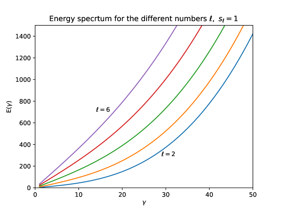
Figure 1: The energy spectrum for the case $L\to\infty$.

We assume that following equality takes place for the real energy $E(\gamma;\ell,s_{\ell})$:

$$E^{\#}(\gamma;\ell,s_{\ell})t^{\#}~{}=~{}E(\gamma;\ell,s_{\ell})t\,.$$

Therefore, the ”real - time” evolution of any vector $|\Psi\rangle\in{\boldsymbol{H}}$ is written as

$$|\Psi\rangle~{}\longrightarrow~{}|\Psi(t)\rangle~{}=~{}\sum_{\Gamma;\ell,s_{\ell}}C_{\gamma;\ell,s_{\ell}}\exp\left(\frac{iE(\gamma;\ell,s_{\ell})\,t}{\hbar}\right)|\Psi(\Gamma;\ell,s_{\ell})\rangle\,,$$

where

$$E(\gamma;\ell,s_{\ell})~{}=~{}\frac{\alpha\,\hbar^{2}}{4\pi^{2}\varrho_{0}R^{4}R_{1}}\left(\frac{R_{0}}{2R_{1}}\,\frac{\gamma^{3}}{{\sf k}_{max}R_{1}}~{}+~{}\gamma\,\ell\sqrt{\ell^{2}-1}\,s_{\ell}\right)\,.$$ (33)

Finally, the numbers $E(\gamma;\ell,s_{\ell})$ give the energy spectrum of our quantum system. The dependence $E=E(\gamma;\ell,s_{\ell})$ is shown in Fig.1 for some conventional scale units.

Of course, the limit $L=\infty$ is unattainable really. Therefore, the ”dimensionless circulation” $\gamma$ takes on a value in discrete set $G_{\epsilon}=(\gamma_{1},\gamma_{2},\dots,\gamma_{n},\dots)$ only. This set $G_{\epsilon}$ is the $\epsilon$-net for the interval $(\zeta_{\,0}^{(0)}\,,{\sf k}_{max}R_{1})$. In accordance with formulas (25) and (27) parameter $\epsilon$ that characterizes the set $G_{\epsilon}$ is defined as follows:

$$\epsilon~{}=~{}\epsilon(m,n,k)~{}=~{}\frac{\pi^{2}}{4}\,\frac{2n+1}{\zeta_{\,k}^{(m)}}\left(\frac{R_{1}}{L}\right)^{2}\,.$$

Thus, the curves that were shown in Fig.1 are not continuous. Really, these curves consist of many nearby points.

4 Concluding remarks

 

As it seems, proposed quantum system is ”inverse realization” of Lord Kelvin’s old idea that any particles can be considered as some kind of vortex-like structures [14]. In our approach, we describe the closed vortex filament as some structured particle. In a sense, the fluid in which the vortex in question moves plays the role of ”aether”. Note that such ”aether” is quite real here, and not hypothetical. It is known that the standard approach to the energy definition of a thin ($a\to 0$) vortex filament leads to problems due to the divergence of integrals. In this study, we applied a group-theoretical approach to the definition of energy. Unfortunately, the author did not find any experimental studies, the results of which could be compared with the formula (33). Hopefully, such studies will appear in the future.

References

- [1] Dirac P.A.M. Generalized hamiltonian dynamics. Canadian Journal of Mathematics. V.2. No 2. pp. 129 - 148 (1950).
- [2] Kastrup H. A. Annalen der Physik. 519. Issues 7-8. 439 - 528 (2007).
- [3] R.J. Donnely. Quantum Vortices in Helium II Cambrige Univ. Press. (1991).
- [4] S.K. Nemirovskii. Gydrodynamics of quantum fluids. Waves, vortices, turbulence. Part II. Quantum vortices, superfluid turbulence. Novisibirsk: Siberian Branch of the Russian Academy of Sciences (2016) In Russian, ISBN 978-5-7692-1482-0
- [5] Sonin E.B. Dynamics of Quantized Vortex in Superfluids. Cambridge University Press (2016).
- [6] P.G. Saffman, Vortex dynamics. Cambrige Univ. Press, (1992).
- [7] S.V. Alekseenko, P.A. Kuibin, V.L. Okulov, Theory of concentrated vortices. Springer-Verlag, Berlin Heidelberg (2007).
- [8] Ricca R.L. Chaos. 3. Issue 1. 83–91 (1993)
- [9] V.F. Kop’ev, S.A. Chernyshev. Vortex ring oscillations, the development of turbulence in vortex rings and generation of sound. Phys. Usp. 43 663–690 (2000).
- [10] L. Kiknadze, Yu. Mamaladze. Journ. Low Temperature Physics. V. 126. Nos 1/2. Jan. (2002).
- [11] A.J. Majda and A.L. Bertozzi. Vorticity and Incompressible Flow. Cambridge Univ. Press. (2002).
- [12] S.V. Talalov. Eur. Journ. Mech B/Fluids. 92. pp. 100 - 106. (2022). arXiv: math-ph/2112.04859v1.
- [13] S.V. Talalov. Phys. Rev. Fluids. 8. 034607 (2023)
- [14] W. Thomson. On vortex atoms. Proc. R. Soc. Edinburgh 6, 94 (1869).