Joint-Embedding Masked Autoencoder for Self-supervised Learning of Dynamic Functional Connectivity from the Human Brain

Abstract

Graph Neural Networks (GNNs) have shown promise in learning dynamic functional connectivity for distinguishing phenotypes from human brain networks. However, obtaining extensive labeled clinical data for training is often resource-intensive, making practical application difficult. Leveraging unlabeled data thus becomes crucial for representation learning in a label-scarce setting. Although generative self-supervised learning techniques, especially masked autoencoders, have shown promising results in representation learning in various domains, their application to dynamic graphs for dynamic functional connectivity remains underexplored, facing challenges in capturing high-level semantic representations. Here, we introduce the Spatio-Temporal Joint Embedding Masked Autoencoder (ST-JEMA), drawing inspiration from the Joint Embedding Predictive Architecture (JEPA) in computer vision. ST-JEMA employs a JEPA-inspired strategy for reconstructing dynamic graphs, which enables the learning of higher-level semantic representations considering temporal perspectives, addressing the challenges in fMRI data representation learning. Utilizing the large-scale UK Biobank dataset for self-supervised learning, ST-JEMA shows exceptional representation learning performance on dynamic functional connectivity demonstrating superiority over previous methods in predicting phenotypes and psychiatric diagnoses across eight benchmark fMRI datasets even with limited samples and effectiveness of temporal reconstruction on missing data scenarios. These findings highlight the potential of our approach as a robust representation learning method for leveraging label-scarce fMRI data.

I Introduction

Recent advancements in neuroimaging research have shown a growing interest in leveraging functional Magnetic Resonance Imaging (fMRI), which captures the Blood-Oxygen-Level-Dependent (BOLD) signal to understand the intricate functionalities of the human brain [16, 37]. Consequently, leveraging fMRI data through Functional Connectivity (FC) has gained traction in addressing various human brain-related problems using neural network models [18]. In this context, FC refers to the temporal correlation degree between Regions of Interest (ROI) s of the brain, enabling the mathematical interpretation of fMRI data as graph structures, where nodes represent ROI s and edges represent the connectivity or correlation between these regions. This enables the utilization of graph-based learning methods such as Graph Neural Network (GNN) to analyze and interpret brain dynamics [11, 17].

While integrating GNN with FC data has marked significant advancements in understanding brain networks, obtaining and labeling clinical fMRI data for supervised learning models poses challenges, affecting the scalability and practical application of these advanced techniques. This challenge highlights the necessity of exploring alternative approaches capable of efficiently leveraging unlabeled data.

In response, utilizing unlabeled fMRI data through Self-Supervised Learning (SSL) presents a promising solution to extract valuable features for downstream tasks [38, 34, 14]. SSL, focused on pre-training backbone models without labels, has driven performance enhancements in diverse domains, including Natural Language Processing (NLP) [10], Image [6, 13], and Video Processing [32]. Among various concepts of SSL methods, generative SSL methods inspired by Masked Language Modeling (MLM) approach [10] have demonstrated superior performance compared to the contrastive learning methods in downstream tasks [13, 32] across a range of different tasks.

This trend towards generative approaches in SSL is also reflected in graph data. GraphMAE [14], for instance, applies a similar philosophy to static graphs, demonstrating that generative SSL can effectively learn foundational models in static graph contexts, surpassing the performance of traditional contrastive learning-based SSL methods. In the context of dynamic graphs, Choi et al. [7] have developed a generative SSL framework that enables foundational models to effectively capture temporal dynamics. When applied to fMRI datasets, this framework demonstrates enhanced performance across multiple downstream tasks, surpassing models based on static graph methodologies and contrastive learning approaches.

While recent advancements in generative SSL have shown improved performance in learning graph data structures, existing methods tend to focus on reconstructing lower-level features [14, 7], potentially limiting their ability to grasp higher-level semantic representations. This learning of low-level features prevents the foundation model from learning the general information required for various downstream tasks in the upstream dataset, which hinders the overall performance after fine-tuning.

To tackle this limitation of current generative SSL methods — reconstructing low-level representation in temporal graph data — we propose a novel framework called Spatio-Temporal Joint Embedding Masked Autoencoder (ST-JEMA) for dynamic graphs such as dynamic functional connectivity of fMRI data. In ST-JEMA, we propose a new joint embedding reconstruction loss based on the latest SSL frameworks known as Joint-Embedding Predictive Architecture (JEPA) [2]. Based on the JEPA-inspired loss function, our method induces the encoder to focus on reconstructing the target input representations rather than the target input features, across both spatial and temporal dimensions. This encourages the GNN models to learn more advanced representations of dynamic graphs.

We employed the extensive UK Biobank fMRI dataset, which consists of 40,913 records, for comparing various SSL methods without demographic characteristics (e.g. Gender), and validated our methodology by fine-tuning across eight benchmarks including non-clinical and clinical fMRI datasets. The experimental results demonstrated that ST-JEMA, by considering temporal dynamics, effectively enhances the learning of node representations in the GNN encoder compared to other baseline SSL methods. This improvement was evident in its superior performance on downstream fMRI tasks.

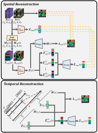
Figure 1: Overview of Spatio-Temporal Joint Embedding Masked Autoencoder framework.

Our key contributions are outlined as follows:

• We introduce ST-JEMA, a novel approach that overcomes the focus on low-level representations in generative SSL by enabling higher-level representation learning in dynamic graphs through JEPA-based reconstruction.

• By employing the extensive fMRI data from the UKB dataset, we achieved enhanced performance across diverse benchmarks, thereby validating the effectiveness of our approach in using large-scale, unlabeled data for backbone GNN models.

• Our proposed method demonstrates enhanced efficacy in scenarios with limited labeled samples, such as with clinical datasets, notably in the data-efficient model development for psychiatric diagnosis classification.

II Related Works

II-A Learning Functional Connectivity of the Brain with Graph Neural Networks

Recent advancements in GNNs have significant interest in understanding brain networks, employing FC networks from fMRI data. Pioneering works have demonstrated the potential of GNNs in enhancing our understanding of functional brain dynamics by addressing the challenges of analyzing large dimensional activation of brain data [36], leveraging ROI-aware GNN architectures [21], and providing generative frameworks [15].

Contrary to the prevalent focus on static FC, there have been efforts to capture the temporal dynamics within fMRI data by proposing temporal dynamic learning [31], modeling temporal variants in brain networks [17], and combining graph structure learning with attention-based graph pooling [22], leveraging the rich temporal variation inherent to such dynamic brain networks. These studies consider temporal variation as an important part of analyzing the brain or determining disorders from fMRI data. In this work, we address the problem of enabling GNN encoders to learn the temporal dynamics inherent in large-scale unlabeled fMRI data by focusing on dynamic graphs.

II-B Self-supervised Learning on Graph Data

Utilizing SSL on graph data has proven to be an effective approach for extracting meaningful representations from large amounts of unlabeled graph data. In the realm of graph contrastive SSL, Deep Graph Infomax [30] and GraphCL [38] have been pioneering efforts that leverage augmentations and multiple graph views to enrich representation learning. However, challenges in augmentation efficacy across domains have led to innovative works, which simplify the process by introducing perturbations to embeddings [39] or model parameters [34]. Generative approaches in graph self-supervised learning focus on reconstructing the original graph structure or node features from encoded representations to capture inherent structural relationships. VGAE [19] employs variational autoencoders for adjacency matrix reconstruction enhancing link prediction performance, while GraphMAE [14] employs a masked autoencoder approach, which shows enhanced performance in node and graph classification compared to previous contrastive methods.

Existing graph self-supervised learning methods are well-established for static graphs but remain less explored for dynamic graphs, especially in learning from dynamic FC, with existing applications mainly in other domains such as traffic flow [11]. Recently, a generative SSL framework designed for dynamic graphs from fMRI data, employing a masked autoencoder for temporal reconstruction, has shown promise in improving downstream task performance [7].

II-C Joint Embedding Predictive Architecture

In the evolving landscape of SSL in computer vision, Assran et al. [2] introduces the JEPA, a new framework that integrates the concepts of both Joint Embedding Architecture (JEA) in contrastive learning and generative learning process of the Masked Autoencoder [MAE; 13]. This approach diverges from the MAE, which mainly focuses on pixel-level image reconstruction. Unlike MAE, which optimizes a decoder to reconstruct parts of masked target image patches from unmasked context patch representations, JEPA aims to avoid the potential pitfall of generating representations overly fixated on low-level details. Instead, Assran et al. [2] utilizes a predictive model trained to infer the representations of masked target patches based on unmasked context patches, enabling the encoder to formulate representations that encapsulate higher-level semantic information beyond mere pixel details. Refer to Appendix Appendix F for more detailed discussions on the related works.

III Preliminaries

III-A Problem Definition

Our goal is to develop a SSL framework capable of effectively capturing the temporal dynamics inherent in dynamic graphs derived from large-scale, unlabeled fMRI data. To achieve this, we utilize SSL strategies to train a GNN encoder and decoder, respectively denoted as $f(\cdot;{\boldsymbol{\theta}})$ and $g(\cdot;{\boldsymbol{\phi}})$, where ${\boldsymbol{\theta}}$ and ${\boldsymbol{\phi}}$ represent the model parameters. The objective is to obtain a pre-trained encoder, $f(\cdot;{\boldsymbol{\theta}}^{*})$, with optimized parameters ${\boldsymbol{\theta}}^{*}$ through SSL using the upstream dataset. Note that the decoder will only be used in pre-training and will be discarded for the finetuning. Still, carefully selecting an appropriate architecture for the decoder remains crucial for effective pre-training of the encoder.

After the pre-training phase, we fine-tune the pre-trained GNN encoder, adding specific prediction heads $h(\cdot;{\boldsymbol{\omega}})$ to solve the tasks on downstream datasets. Given the limited number of labeled data for the downstream training dataset, it is crucial to ensure that the encoder and prediction head, avoid overfit to the downstream data and achieve good generalization performance to unseen datasets. The key lies in finding a well-pre-trained encoder $f(\cdot;{\boldsymbol{\theta}}^{*})$ that captures the key patterns and dynamics within the fMRI data, which facilitates a comprehensive understanding of the fMRI dataset.

III-B Notations for Dynamic Graphs

A graph ${\mathcal{G}}$ is defined as ${\mathcal{G}}=({\mathcal{V}},{\mathcal{E}})$, where ${\mathcal{V}}$ denotes a set of vertices or nodes, and ${\mathcal{E}}$ denotes a set of edges or links between these vertices. The set ${\mathcal{E}}$ is defined as ${\mathcal{E}}=\{e_{ij}\,|\,i,j\in\{1,\cdots,N\},\text{ and }j\in{\mathcal{N}}(i)\}$, where $N$ is the number of nodes $|{\mathcal{V}}|$ and ${\mathcal{N}}(i)$ is the neighborhood of node $i$. Here, $e_{ij}$ indicates a relationship or connection between node $i$ and node $j$. Each node in ${\mathcal{V}}$ represents an individual entity, characterized by its feature vector $\boldsymbol{x}\in\mathbb{R}^{d_{v}}$, where $d_{v}$ indicates the dimensionality of the node feature space.

Additionally, the adjacency matrix $\boldsymbol{A}$ plays a crucial role as an edge feature in GNN. It represents the presence or absence of connections between nodes, thereby facilitating message passing that considers the relationships between nodes. Mathematically, the adjacency matrix is defined as

$$\boldsymbol{A}=(a_{i,j})\in\{0,1\}^{N\times N}.$$ (1)

Here, $a_{ij}=1$ when $e_{i,j}\in{\mathcal{E}}$, and otherwise 0 for all $i,j\in[N]$.

Dynamic Graph. In real-world graph datasets, there are two types of datasets: 1) static graph datasets and 2) dynamic graph datasets. Static graph datasets contain time-independent graph data that remains unchanged over time. In contrast, dynamic graph datasets include time-dependent graph data that evolves as time progresses. For dynamic graphs, it becomes crucial to consider the dynamic nature when examining numerous real-world graph data scenarios, particularly in the context of studying the functionalities of the human brain [17]. Here, a dynamic graph can be denoted as a series of evolving graphs ${\mathcal{G}}(t)=({\mathcal{V}}(t),{\mathcal{E}}(t))$ over discrete time points $t\in{\mathcal{T}}$. Each ${\mathcal{G}}(t)$ also include node features $\boldsymbol{X}(t)\in\mathbb{R}^{N\times d_{v}}$ and an adjacency matrix $\boldsymbol{A}(t)$ corresponding to the time point $t$.

III-C Constructing Dynamic Graphs from fMRI data

fMRI data are complex and multidimensional, consisting of a sequence of brain images represented in 3D voxels collected over time. Each voxel within these images stands for a tiny volume in the brain, and the value of each voxel reflects the intensity of the BOLD signal at that particular location and time. In this study, we focus on neural activity within predefined ROI, Schaefer atlas [25], leveraging its comprehensive partitioning of the cerebral cortex into functionally homogeneous regions. We construct the ROI-based BOLD signal data matrix $\boldsymbol{P}\in\mathbb{R}^{N\times T_{max}}$, with $N$ representing the number of ROI and $T_{max}$ the time points, by averaging BOLD signals within each ROI. This simplification retains essential details for subsequent dynamic functional connectivity analysis.

To analyze the BOLD signal with GNN, we construct dynamic graphs from the ROI-time-series matrix $\boldsymbol{P}$ of resting state fMRI (rs-fMRI) by defining node features $\boldsymbol{X}$ and the adjacency matrix $\boldsymbol{A}$. In this study, we utilize rs-fMRI because it allows for the exploration of spontaneous brain activity in the absence of task performance, offering insights into the brain’s intrinsic functional connectivity from understanding fundamental brain networks to predicting phenotypes such as gender or disease presence. For node feature $\boldsymbol{X}$, the ROI-time-series matrix $\boldsymbol{P}$ serves as the basis for generating node features that capture their temporal dynamics. Each node features $\boldsymbol{x}$ is combined spatial embeddings with learned temporal encodings using concatenation operation $\|$. Specifically, the feature vector of $i$-th node at time $t$ is formulated as:

$$\boldsymbol{x}_{i}(t)=\boldsymbol{W}[\boldsymbol{e}_{i}\,\|\,{\boldsymbol{\eta}}(t)],$$ (2)

where $\boldsymbol{W}\in\mathbb{R}^{{d_{v}}\times(N+{d_{\eta}})}$ is a learnable parameter matrix, $\boldsymbol{e}_{i}$ denotes the one-hot spatial embedding of the $i$-th node, and ${\boldsymbol{\eta}}(t)\in\mathbb{R}^{d_{\eta}}$ is the temporal encoding obtained through a Gated Recurrent Unit (GRU) [8]. Here, $d_{\eta}$ refers to the dimensionality of the temporal encoding. This temporal encoding is designed to capture the dynamic changes in BOLD signals within each ROI over time, thus incorporating temporal variations into the node features. Now, the final node feature matrix $\boldsymbol{X}(t)$ can be defined as a stack of node feature vectors at time $t$:

$$\boldsymbol{X}(t)=\begin{bmatrix}|&&|\\ \boldsymbol{x}_{1}(t)&\cdots&\boldsymbol{x}_{N}(t)\\ |&&|\end{bmatrix}.$$ (3)

For the adjacency matrix $\boldsymbol{A}(t)$, we derive the FC between ROI based on the temporal correlation of BOLD signal changes, utilizing the ROI-timeseries matrix $\boldsymbol{P}$. The FC matrix at time $t$, $\boldsymbol{R}(t)$, is calculated as follows:

$$R_{ij}(t)=\frac{\text{Cov}(\bar{\boldsymbol{p}}_{i}(t),\bar{\boldsymbol{p}}_{j}(t))}{\sqrt{\smash[b]{\text{Var}(\bar{\boldsymbol{p}}_{i}(t))}}\sqrt{\smash[b]{\text{Var}(\bar{\boldsymbol{p}}_{j}(t))}}}\in\mathbb{R}^{N\times N},$$ (4)

where $\bar{\boldsymbol{p}}_{i}(t)$ and $\bar{\boldsymbol{p}}_{j}(t)$ are the BOLD signal vectors for nodes $i$ and $j$ within the temporal windowed matrix $\bar{\boldsymbol{P}}(t)\in\mathbb{R}^{N\times\Gamma}$ from $\boldsymbol{P}$, characterized by a temporal window length of $\Gamma$ and stride $S$. Here, $t\in[T_{\mathcal{G}}]$ where $T_{\mathcal{G}}=\lfloor(T_{\text{max}}-\Gamma)/S\rfloor$. Cov denotes the covariance, and Var represents the variance operation. The adjacency matrix $\boldsymbol{A}(t)\in\{0,1\}^{N\times N}$ is then obtained by applying a threshold to the correlation matrix $\boldsymbol{R}(t)$, wherein the top 30-percentile values are considered as significant connections (1), and all others are considered as non-significant (0).

III-D Context and Target for Reconstruction

Our method expands generative SSL upon the idea of JEPA, which reconstructs the latent representation space instead of the input feature space, within the domain of dynamic graphs derived from fMRI data. Assran et al. [2] employs a multi-block masking strategy for target block prediction, where it simultaneously utilizes $K$ different masks for a single image data. Adapting JEPA concepts to dynamic graph scenarios involves treating each masked section of the graph as targets while considering the remaining areas as contexts. Within a graph ${\mathcal{G}}(t)$ at a specific time $t$, we distinguish between masked target nodes and unmasked context nodes as follows:

$$\begin{gathered}\boldsymbol{X}^{(k)}_{\texttt{cxt}}(t)=\{\boldsymbol{x}_{i}(t)\mid i\in[N],\boldsymbol{M}^{(k)}_{\boldsymbol{X},i}(t)=\mathbf{1}_{d_{v}}\},\\ \boldsymbol{X}^{(k)}_{\texttt{tar}}(t)=\{\boldsymbol{x}_{i}(t)\mid i\in[N],\boldsymbol{M}^{(k)}_{\boldsymbol{X},i}(t)=\mathbf{0}_{d_{v}}\},\end{gathered}$$ (7)

where $k\in[K]$ and $\boldsymbol{M}_{\boldsymbol{X}}^{(k)}(t)=\{0,1\}^{\mathbb{R}^{N\times d_{v}}}$ is the $k$-th binary mask with the same shape as $\boldsymbol{X}(t)$ at time $t\in[T_{{\mathcal{G}}}]$. Here, $\mathbf{1}_{d_{v}}$ represents a vector of ones, and $\mathbf{0}_{d_{v}}$ represents a vector of zeros, indicating masked and unmasked node features, respectively.

Similarly, the adjacency matrix $\boldsymbol{A}(t)$ is partitioned into context and target components. The context parts of the adjacency matrix are used to extract node embeddings of GNN in combination with the context node features. These embeddings are then applied to reconstruct each target component of the adjacency matrix.

IV Methods

IV-A Joint Embedding Architecture

To enhance GNN encoder to capture higher-level semantic information in spatial and temporal patterns, we have introduced a new JEPA-inspired reconstruction strategy, utilizing dual encoders and decoders. The encoders, designated as $f_{\texttt{cxt}}(\cdot;{\boldsymbol{\theta}})$ for context and $f_{\texttt{tar}}(\cdot;\bar{{\boldsymbol{\theta}}})$ for target, encode the context and target components, respectively, with ${\boldsymbol{\theta}}$ representing the learnable parameters for the context encoder and $\bar{{\boldsymbol{\theta}}}$ for the target encoder, which is updated based on ${\boldsymbol{\theta}}$. Meanwhile, the decoders, named $g_{\texttt{node}}(\cdot;{\boldsymbol{\phi}}_{\mathcal{V}})$ and $g_{\texttt{edge}}(\cdot;{\boldsymbol{\phi}}_{{\mathcal{E}}})$, aim to reconstruct the target nodes’ representations and the adjacency matrix, respectively. Here, ${\boldsymbol{\phi}}_{\mathcal{V}}$ and ${\boldsymbol{\phi}}_{{\mathcal{E}}}$ denote the parameters of each decoder, respectively.

Employing separate encoders for context and target components is crucial to prevent representation collapse [12] during training [2]. Although these encoders share identical structural designs, they follow distinct parameter update rules. Specifically, the context encoder $f_{\texttt{cxt}}$ is updated via Stochastic Gradient Descent (SGD), driven by subsequent reconstruction loss objectives, while the target encoder $f_{\texttt{tar}}$ remains frozen. Subsequently, The parameters of target encoder, $\bar{{\boldsymbol{\theta}}}$, are then updated using Exponential Moving Average (EMA) based on the evolving parameters of $f_{\texttt{cxt}}$ as follows:

$$\bar{{\boldsymbol{\theta}}}_{\text{new}}=\beta\bar{{\boldsymbol{\theta}}}_{\text{old}}+(1-\beta){\boldsymbol{\theta}}_{\text{cxt}},$$ (8)

where hyperparameter $\beta\in[0,1]$ represents the decay factor. Here, $\bar{{\boldsymbol{\theta}}}_{\text{old}}$ and $\bar{{\boldsymbol{\theta}}}_{\text{new}}$ refer to the parameters of $f_{\texttt{tar}}$ before and after applying EMA process, respectively, and ${\boldsymbol{\theta}}_{\text{ctx}}$ indicates the current parameters of $f_{\texttt{cxt}}$. Adopting distinct update rules for each encoder, as outlined, serves to prevent the encoders from capturing simplistic and non-informative trivial representations. This approach allows us to harness GNN encoder to learn high-level semantic representations while maintaining nearly the same computational demand during back-propagation.

IV-B Block Masking Process for Masked Autoencoding

To effectively train spatial and temporal patterns across individual time steps $t$, suitable masks need to be applied to both the node features and the adjacency matrix $\big{(}\boldsymbol{X}(t),\boldsymbol{A}(t)\big{)}$, resulting in masked versions $\big{(}\boldsymbol{X}_{\texttt{cxt}}(t),\boldsymbol{A}_{\texttt{cxt}}(t)\big{)}$ for each time step $t$.

As presented in Assran et al. [2], when training a model with a JEPA-based masked autoencoding objective, a sufficiently large size of the target masks, with sequential indices, is crucial in the image dataset. This strategy ensures that the masked targets encompass meaningful semantic information, allowing models to grasp the semantic structure by reconstructing the target data from the remaining context. Although this can be easily done by masking the patch for the image data, applying similar masking techniques to nodes and edges in graph data is challenging due to the absence of clear relationships between sequential indices for nodes. However, in the context of dynamic FC of fMRI data, the graph construction method outlined in Kim et al. [17] defines a well-aligned construction between nodes with adjacent indices across time. Consequently, masking nodes with sequential indices is a natural and effective approach for the dynamic FC of fMRI data. This method allows for the masking of nodes without sacrificing meaningful semantic information.

As mentioned earlier, generating adequately sized masks for both nodes and edges at each time step $t$ is essential to capture meaningful semantic information within the masked blocks. To achieve this for node features $\boldsymbol{X}(t)$, we generate $K$ binary mask matrices $\boldsymbol{M}_{\boldsymbol{X}}^{(k)}(t)$, where each $\boldsymbol{M}_{\boldsymbol{X}}^{(k)}(t)$ randomly and independently masks a $\lfloor\alpha_{\texttt{node}}^{(k)}(t)\cdot N\rfloor$ number of nodes with sequential indices. Here, mask ratio $\alpha_{\texttt{node}}^{(k)}(t)$ uniformly sampled from $(\alpha_{\text{min}},\alpha_{\text{max}})$ where $0<\alpha_{\text{min}}<\alpha_{\text{max}}<1$ are predefined hyperparameters. This process ensures the creation of appropriately sized blocks. Refer to Appendix Section E-B for the experimental results regarding the ablation study on block mask ratios.

After generating $K$ distinct masks, when creating context node features for each target node feature, the memory requirements for context node features increase linearly with the growth of $K$. To remedy this issue, we employ a single global context node feature for each time $t$, outlined as follows:

$$\boldsymbol{X}_{\texttt{cxt}}(t)=\boldsymbol{X}(t)\odot\bigg{(}\boldsymbol{M}^{(1)}_{\boldsymbol{X}}(t)\odot\ldots\odot\boldsymbol{M}^{(K)}_{\boldsymbol{X}}(t)\bigg{)},$$ (9)

where $\odot$ denotes elementwise product.

For the adjacency matrix $\boldsymbol{A}(t)$, we also construct $K$ binary masks $\boldsymbol{M}_{\boldsymbol{A}}^{(k)}(t)$ for $k\in[K]$ in a similar fashion. The distinction in constructing an adjacency matrix mask primarily involves blocking a randomly chosen square-shaped submatrix. To create a mask $\boldsymbol{M}_{\boldsymbol{A}}^{(k)}(t)$ by sampling a square-shaped submatrix from the adjacency matrix, we independently and randomly select two sets of sequential indices $I_{1}$ and $I_{2}$. These sets have the same cardinality of $\lfloor\alpha_{\texttt{adj}}^{(k)}(t)\cdot N\rfloor$, where $\alpha_{\texttt{adj}}^{(k)}(t)$ is uniformly sampled from $(\alpha_{\text{min}},\alpha_{\text{max}})$. Subsequently, we nullify the $(i,j)$th entry of $\boldsymbol{M}_{\boldsymbol{A}}^{(k)}(t)$ for all $i\in I_{1}$ and $j\in I_{2}$. Following the independent and random construction of $K$ adjacency matrix masks, akin to node features, we utilize a single global context adjacency matrix for each time $t$, described as follows:

$$\boldsymbol{A}_{\texttt{cxt}}(t)=\boldsymbol{A}(t)\odot\bigg{(}\boldsymbol{M}^{(1)}_{\boldsymbol{A}}(t)\odot\ldots\odot\boldsymbol{M}^{(K)}_{\boldsymbol{A}}(t)\bigg{)}.$$ (10)

The aforementioned masking strategies for the node features and the adjacency matrix encourage the model to learn the underlying brain connectivity patterns for each time $t$ thereby enhancing the understanding of dynamics in the spatial dimension.

IV-C Spatial Reconstruction Process

Based on the masks generated from Section IV-B, we introduce an objective function inspired by JEPA, referred to as ${\mathcal{L}}_{\texttt{spat}}$, aiming to facilitate the learning of spatial patterns within the dynamic FC of fMRI data using GNN representations. To create ${\mathcal{L}}_{\texttt{spat}}$, we need to reconstruct the target node representations and the target adjacency matrix based on the context node representations and the context adjacency matrix. To achieve this reconstruction, we initially build the common context node representation for each time $t$ as follows:

$$\boldsymbol{Z}(t)=f_{\texttt{cxt}}\Big{(}\boldsymbol{X}_{\texttt{cxt}}(t),\boldsymbol{A}_{\texttt{cxt}}(t);{\boldsymbol{\theta}}\Big{)}.$$ (11)

Here, we can employ any GNN models capable of accepting node features and adjacency matrices as input for our $f_{\texttt{cxt}}$. To reconstruct the target node representations using only the context node representations, we reapply masking to the context node representations at the indices corresponding to the masked target node representations. This results in generating masked context node representations $\tilde{\boldsymbol{Z}}_{\texttt{cxt}}(t)$ computed as follows:

$$\begin{gathered}\tilde{\boldsymbol{Z}}(t)=\boldsymbol{W}_{\texttt{S}}^{{\mathcal{V}}}\boldsymbol{Z}(t),\\ \tilde{\boldsymbol{Z}}_{\texttt{cxt}}(t)=\tilde{\boldsymbol{Z}}(t)\odot\Big{(}\boldsymbol{M}_{\boldsymbol{X}}^{(1)}(t)\odot\cdots\odot\boldsymbol{M}_{\boldsymbol{X}}^{(K)}(t)\Big{)},\end{gathered}$$ (14)

where $\boldsymbol{W}_{\texttt{S}}^{{\mathcal{V}}}\in\mathbb{R}^{d_{\texttt{dec}}\times d_{\texttt{enc}}}$ denotes a learnable projection matrix that is used to adjust from the encoder dimension $d_{\texttt{enc}}$ to the decoder dimension $d_{\texttt{dec}}$. Using the masked context node representations $\tilde{\boldsymbol{Z}}(t)$ and any node mask $\boldsymbol{M}_{\boldsymbol{X}}^{(k)}(t)$, we derive the target-specific context node representations $\tilde{\boldsymbol{Z}}_{\texttt{cxt}}^{(k)}(t)$ as follows:

$$\begin{gathered}\tilde{\boldsymbol{Z}}_{\texttt{cxt}}^{(k)}(t)=\tilde{\boldsymbol{Z}}_{\texttt{cxt}}(t)+\boldsymbol{m}\cdot\Big{(}\mathds{1}_{\boldsymbol{X}}-\boldsymbol{M}_{\boldsymbol{X}}^{(k)}(t)\Big{)},\end{gathered}$$ (16)

where $\mathds{1}_{\boldsymbol{X}}$ represents a matrix filled with ones having the same shape as $\boldsymbol{M}^{(k)}_{\boldsymbol{X}}(t)$, and $\boldsymbol{m}\in\mathbb{R}^{d_{\texttt{dec}}}$ denotes a learnable mask vector conditioning the target block we wish to reconstruct following Assran et al. [2]. This vector is crucial for conditioning the specific target block among $K$ mask blocks from the single global context node representation $\tilde{\boldsymbol{Z}}_{\texttt{cxt}}(t)$.

In summary, these target-specific context node representations $\tilde{\boldsymbol{Z}}_{\texttt{cxt}}^{(k)}(t)$ are set to zero for all target node representations belonging to $K-1$ masks, except for those associated with the $k$-th mask. For the latter, corresponding representations are set to the values from the learnable mask vector $\boldsymbol{m}$. Then finally with this target-specific context node representation $\tilde{\boldsymbol{Z}}_{\texttt{cxt}}^{(k)}(t)$, we recover the target node representation $\hat{\boldsymbol{Z}}_{\texttt{tar}}^{(k)}(t)$ for the $k$-th mask as follows:

$$\hat{\boldsymbol{Z}}_{\texttt{tar}}^{(k)}(t)=g_{\texttt{node}}\bigg{(}\tilde{\boldsymbol{Z}}_{\texttt{cxt}}^{(k)}(t);{\boldsymbol{\phi}}_{\mathcal{V}}\bigg{)}.$$ (17)

For the architecture of $g_{\texttt{node}}$, we opt for the MLP-Mixer [29] architecture. This choice is different from the usual selection of a Multi-Layer Perceptron (MLP) as the decoder for the graph SSL. In contrast to a simple MLP structure, the MLP-Mixer structure facilitates interactions among all nodes, enabling the reconstruction of the target node’s representation by fully considering the representations of context nodes.

Our target node representations for the $k$-th mask $\boldsymbol{Z}_{\texttt{tar}}^{(k)}(t)$ is computed with unmasked $\boldsymbol{X}(t)$ and $\boldsymbol{A}(t)$:

$$\begin{gathered}\boldsymbol{Z}_{\texttt{tar}}(t)=f_{\texttt{tar}}\bigg{(}\boldsymbol{X}(t),\boldsymbol{A}(t);\bar{{\boldsymbol{\theta}}}\bigg{)},\\ \boldsymbol{Z}_{\texttt{tar}}^{(k)}(t)=\boldsymbol{Z}_{\texttt{tar}}(t)\odot\Big{(}\mathds{1}_{\boldsymbol{X}}-\boldsymbol{M}_{\boldsymbol{X}}^{(k)}(t)\Big{)}.\end{gathered}$$ (20)

Then finally our node reconstruction objective ${\mathcal{L}}_{\texttt{node-spat}}^{(t)}$ at time $t$ is computed as follows:

$${\mathcal{L}}_{\texttt{node-spat}}^{(t)}=\frac{1}{K}\sum_{k\in[K]}{\mathcal{L}}_{\texttt{MSE}}\Big{(}\hat{\boldsymbol{Z}}_{\texttt{tar}}^{(k)}(t),\boldsymbol{Z}_{\texttt{tar}}^{(k)}(t)\Big{)},$$ (21)

where ${\mathcal{L}}_{\texttt{MSE}}$ denotes the Mean Squared Error (MSE) loss. In contrast to prior graph-based MAE methods [28, 14], where the entire node representations are recovered by the decoder module, our approach only focuses on recovering the target node representations. This strategy guides the model to concentrate on learning spatial patterns by specifically emphasizing the retrieval of semantic information embedded within the masked target nodes.

To recover the adjacency matrix at time $t$, we used the common context node representation $\boldsymbol{Z}(t)$. Based on the reconstruction approach in Kipf and Welling [19], our reconstructed target adjacency matrix $\hat{\boldsymbol{A}}_{\texttt{tar}}^{(k)}(t)$ for the $k$-th mask $\boldsymbol{M}^{(k)}_{\boldsymbol{A}}(t)$ at time $t$ computed as follows:

$$\begin{gathered}\boldsymbol{H}(t)=g_{\texttt{edge}}\Big{(}\boldsymbol{W}_{\texttt{S}}^{\mathcal{E}}\boldsymbol{Z}(t);{\boldsymbol{\phi}}_{\mathcal{E}}\Big{)},\\ \hat{\boldsymbol{A}}_{\texttt{tar}}^{(k)}(t)=\texttt{sig}\Big{(}\boldsymbol{H}(t)\boldsymbol{H}(t)^{\top}\Big{)}\odot\Big{(}\mathds{1}_{\boldsymbol{A}}-\boldsymbol{M}_{\boldsymbol{A}}^{(k)}(t)\Big{)},\end{gathered}$$ (24)

where $\mathds{1}_{\boldsymbol{A}}$ represents a matrix filled with ones having the same shape as $\boldsymbol{M}^{(k)}_{\boldsymbol{A}}(t)$, and sig is an element-wise sigmoid function. We also apply a learnable projection matrix $\boldsymbol{W}_{\texttt{S}}^{\mathcal{E}}\in\mathbb{R}^{d_{\texttt{dec}}\times d_{\texttt{enc}}}$ to adjust dimensions from the encoder to the decoder. And our target adjacency submatrix $\boldsymbol{A}_{\texttt{tar}}^{(k)}(t)$ for the $k$-th mask at time $t$ is simply computed as:

$$\boldsymbol{A}_{\texttt{tar}}^{(k)}(t)=\boldsymbol{A}(t)\odot\Big{(}\mathds{1}_{\boldsymbol{A}}-\boldsymbol{M}_{\boldsymbol{A}}^{(k)}(t)\Big{)}.$$ (25)

Then our adjacency matrix reconstruction loss ${\mathcal{L}}_{\texttt{adj-spat}}^{(t)}$ at time $t$ is computed as follows:

$${\mathcal{L}}_{\texttt{adj-spat}}^{(t)}=\frac{1}{K}\sum_{k\in[K]}{\mathcal{L}}_{\texttt{BCE}}\Big{(}\hat{\boldsymbol{A}}_{\texttt{tar}}^{(k)}(t),\boldsymbol{A}_{\texttt{tar}}^{(k)}(t)\Big{)},$$ (26)

where ${\mathcal{L}}_{\texttt{BCE}}$ denote the Binary Cross-Entropy (BCE) loss function.

In summary, our overall loss function ${\mathcal{L}}_{\texttt{spat}}$ to capture and learn the spatial patterns is formulated as:

$${\mathcal{L}}_{\texttt{spat}}=\sum_{t\in{\mathcal{T}}}\bigg{(}\lambda_{\texttt{node}}{\mathcal{L}}_{\texttt{node-spat}}^{(t)}+\lambda_{\texttt{adj}}{\mathcal{L}}_{\texttt{adj-spat}}^{(t)}\bigg{)},$$ (27)

where $\lambda_{\texttt{node}}$ and $\lambda_{\texttt{adj}}$ serve as hyperparameters regulating the scales of the two individual loss terms.

IV-D Temporal Reconstruction Process

To enhance the understanding of temporal dynamics within the dynamic FC of fMRI data, we also construct a JEPA-based ${\mathcal{L}}_{\texttt{temp}}$. This temporal reconstruction strategy is designed to predict node representations and adjacency matrices at a specific time $t$ by utilizing node representation from two random points in time, $t_{a}$ and $t_{b}$, that can encompass $t$ within their interval. For the selection of $t_{a}$ and $t_{b}$, we adopt a uniform sampling strategy following Choi et al. [7], a straightforward method for choosing two temporal points. An important consideration when sampling $t_{a}$ and $t_{b}$ is the use of a temporal windowing process with a length of $\Gamma$ and a stride of $S$ when constructing a series of FC matrices from the BOLD signal, as discussed in Section III-C. If $t_{a}$ and $t_{b}$ are sampled too closely, there may be an overlap between the windows of $t_{a}$ and $t_{b}$, making the reconstruction task trivial. To ensure the challenge and effectiveness of the temporal reconstruction task, we take care to ensure that the sampled time points $t_{a}$ and $t_{b}$ do not originate from overlapping windows as follows:

$$t_{a}\overset{\text{i.i.d.}}{\sim}U_{\text{int}}([0,t-d_{\text{min}}]),\quad t_{b}\overset{\text{i.i.d.}}{\sim}U_{\text{int}}([t+d_{\text{min}},T_{\mathcal{G}}]),$$ (28)

where $t$ is a target timestep, $U_{\text{int}}(I)$ is a uniform distribution for all integer values in interval $I$ and $d_{\text{min}}=\frac{1}{2}(\frac{\Gamma}{S}+1)$.

Then we first reconstruct the target node representations $\bar{\boldsymbol{Z}}_{\texttt{tar}}^{(k)}(t)$ for the $k$-th mask at time $t$ utilizing $\boldsymbol{Z}(t_{a})$ and $\boldsymbol{Z}(t_{b})$ which are the context node representation at time $t_{a}$ and time $t_{b}$, respectively. To aggregate $\boldsymbol{Z}(t_{a})$ and $\boldsymbol{Z}(t_{b})$ into single node representation $\tilde{\boldsymbol{Z}}_{a,b}(t)$, we compute the $\tilde{\boldsymbol{Z}}_{a,b}(t)$ as follows:

$$\tilde{\boldsymbol{Z}}_{a,b}(t)=\boldsymbol{W}_{\texttt{T}}\Big{[}\tilde{\boldsymbol{Z}}(t_{a})\,\|\,\tilde{\boldsymbol{Z}}(t_{b})\Big{]},$$ (29)

where, $\boldsymbol{W}_{\texttt{T}}\in\mathbb{R}^{d_{\texttt{dec}}\times 2d_{\texttt{enc}}}$ denotes a learnable projection matrix. Instead of employing a learnable mask vector to fill the masked target node representations at $\tilde{\boldsymbol{Z}}(t)$ , as described in Eq. 16, we utilize node representations from $t_{a}$ and $t_{b}$ to construct the target-specific context node representations $\bar{\boldsymbol{Z}}_{\texttt{cxt}}^{(k)}(t)$ for the $k$-th mask at time $t$ as follows:

$$\bar{\boldsymbol{Z}}_{\texttt{cxt}}^{(k)}(t)=\tilde{\boldsymbol{Z}}_{\texttt{cxt}}(t)+\tilde{\boldsymbol{Z}}_{a,b}(t)\odot\Big{(}\mathds{1}_{\boldsymbol{X}}-\boldsymbol{M}_{\boldsymbol{X}}^{(k)}(t)\Big{)}.$$ (30)

Employing $\boldsymbol{Z}_{a,b}(t)$ to populate the target node representations encourages our model to better grasp the temporal dynamics within the data, enhancing its understanding of temporal variations. Then our final recovered target node representations $\bar{\boldsymbol{Z}}_{\texttt{tar}}^{(k)}(t)$ is computed as below:

$$\bar{\boldsymbol{Z}}_{\texttt{tar}}^{(k)}(t)=g_{\texttt{node}}\bigg{(}\bar{\boldsymbol{Z}}_{\texttt{cxt}}^{(k)}(t);{\boldsymbol{\phi}}_{\mathcal{V}}\bigg{)}.$$ (31)

Here, we used the same decoder $g_{\texttt{node}}$ within the spatial reconstruction. Our temporal node reconstruction loss ${\mathcal{L}}_{\texttt{node-temp}}^{(t)}$ at time $t$ is computed as:

$${\mathcal{L}}_{\texttt{node-temp}}^{(t)}=\frac{1}{K}\sum_{k\in[K]}{\mathcal{L}}_{\texttt{MSE}}\Big{(}\bar{\boldsymbol{Z}}_{\texttt{tar}}^{(k)}(t),\boldsymbol{Z}_{\texttt{tar}}^{(k)}(t)\Big{)}.$$ (32)

For the adjacency matrix reconstruction task, we use $\boldsymbol{Z}(t_{a})$ and $\boldsymbol{Z}(t_{b})$ in different ways from the spatial reconstruction. We first construct each $\boldsymbol{H}(t_{a})$ and $\boldsymbol{H}(t_{b})$ using $\boldsymbol{Z}(t_{a})$ and $\boldsymbol{Z}(t_{b})$, respectively. Then compute the reconstructed adjacency matrix for time $t$ as:

$$\bar{\boldsymbol{A}}_{\texttt{tar}}(t)=\frac{1}{2}\bigg{(}\texttt{sig}(\tilde{\boldsymbol{A}}_{ab})+\texttt{sig}(\tilde{\boldsymbol{A}}_{ba})\bigg{)},$$ (33)

where $\tilde{\boldsymbol{A}}_{ab}=\boldsymbol{H}(t_{a})\boldsymbol{H}(t_{b})^{\top}$ and $\tilde{\boldsymbol{A}}_{ba}=\boldsymbol{H}(t_{b})\boldsymbol{H}(t_{a})^{\top}$. Utilizing matrix multiplication between $\boldsymbol{H}(t_{a})$ and $\boldsymbol{H}(t_{b})$ to reconstruct the adjacency matrix also aids our model in effectively learning complex temporal dynamics within dynamic graph data [7].

Our reconstructed target adjacency submatrix $\bar{\boldsymbol{A}}_{\texttt{tar}}^{(k)}(t)$ for the $k$-th mask at time $t$ formulated as:

$$\bar{\boldsymbol{A}}_{\texttt{tar}}^{(k)}(t)=\bar{\boldsymbol{A}}_{\texttt{tar}}(t)\odot\Big{(}\mathds{1}_{\boldsymbol{A}}-\boldsymbol{M}_{\boldsymbol{A}}^{(k)}(t)\Big{)}.$$ (34)

Therefore our temporal adjacency matrix reconstruction loss ${\mathcal{L}}_{\texttt{adj-temp}}^{(t)}$ can be computed as follows:

$${\mathcal{L}}_{\texttt{adj-temp}}^{(t)}=\frac{1}{K}\sum_{k\in[K]}{\mathcal{L}}_{\texttt{BCE}}\Big{(}\bar{\boldsymbol{A}}_{\texttt{tar}}^{(k)}(t),\boldsymbol{A}_{\texttt{tar}}^{(k)}(t)\Big{)},$$ (35)

In summary, our overall loss function ${\mathcal{L}}_{\texttt{temp}}$ to understand the temporal patterns is formulated as:

$${\mathcal{L}}_{\texttt{temp}}=\sum_{t\in{\mathcal{T}}}\bigg{(}\lambda_{\texttt{node}}{\mathcal{L}}_{\texttt{node-temp}}^{(t)}+\lambda_{\texttt{adj}}{\mathcal{L}}_{\texttt{adj-temp}}^{(t)}\bigg{)}.$$ (36)

Here, we use same $\lambda_{\texttt{node}}$ and $\lambda_{\texttt{adj}}$ within ${\mathcal{L}}_{\texttt{spat}}$.

IV-E Summary of the Overall ST-JEMA Pipeline

During each training step, we calculate both the spatial reconstruction loss, ${\mathcal{L}}_{\texttt{spat}}$, and the temporal reconstruction loss, ${\mathcal{L}}_{\texttt{temp}}$. These two distinct loss components are then aggregated to formulate the combined objective function, ${\mathcal{L}}_{\texttt{ST-JEMA}}$, as follows:

$${\mathcal{L}}_{\texttt{ST-JEMA}}=\gamma{\mathcal{L}}_{\texttt{spat}}+(1-\gamma){\mathcal{L}}_{\texttt{temp}},$$ (37)

where the hyperparameter $\gamma\in[0,1]$ is the ratio of ${\mathcal{L}}_{\texttt{spat}}$. The overview and complete training pipeline of the Spatio-Temporal Joint Embedding Masked Autoencoder (ST-JEMA) are described in Fig. 1 and Appendix Appendix A.

V Experimental Setup

We utilize the UKB [27] as the upstream dataset, a large-scale fMRI data comprised of 40,913 subjects, for pre-training GNN encoder with SSL. We evaluate the pre-trained GNN encoder across eight downstream datasets both non-clinical and clinical rs-fMRI datasets. For non-clinical datasets, we evaluate gender classification and age regression tasks using ABCD  [5], and three types of HCP datasets: HCP-YA [33], HCP-A [3], and HCP-D [26]. For clinical datasets, we extended psychiatric diagnosis classification tasks to distinguish between normal control groups and different psychiatric disorder groups using HCP-EP [20], ABIDE [9], ADHD200 [4], and COBRE [23].

To show effectiveness of ST-JEMA, we compared these downstream performance against previous SSL methods including both static graphs (DGI [30], SimGRACE [34], GAE [19], VGAE [19], GraphMAE [14]) and dynamic graphs (ST-DGI [24], ST-MAE [7]).

The training process was divided into two phases: 1) pre-training, where a GNN encoder $f(;{\boldsymbol{\theta}})$ and decoder $g(;{\boldsymbol{\phi}})$ were learned using SSL on the UKB dataset without phenotype labels, employing a 4-layer GIN [35] for encoder module and a one-layer MLP-mixer for the decoder in the ST-JEMA framework, and 2) fine-tuning, where the pre-trained encoder and a task-specific head $h(;{\boldsymbol{\omega}})$, incorporating the SERO readout module[17], were further trained on downstream tasks with supervised learning. Pre-training employed a cosine decay learning schedule over 10K steps with a batch size of 16. Fine-tuning optimized the encoder with the task-specific head, using orthogonal regularization and a one-cycle scheduler for 30 epochs with a batch size of 32. Dynamic graphs integrated a mean pooling module for final representation processing. Classification tasks used cross-entropy loss, while age regression utilized MSE loss with normalized age data. The training utilized AMD EPYC processors, with NVIDIA RTX A6000 for pre-training and GeForce RTX 3090 for fine-tuning and ablation studies.

For further details on the experimental setup, please refer to Appendix Appendix B, Appendix C, and Appendix D.

VI Results

TABLE I: Gender classification performance across various downstream fMRI datasets. The performance is evaluated using the AUROC score, with higher scores indicating better performance.

Type of FC Pre-training Method Type AUROC ($\uparrow$) Rank ABCD HCP-YA HCP-A HCP-D HCP-EP ABIDE ADHD200 COBRE Static Random-Init Supervised 72.74 86.93 68.48 66.22 55.54 69.62 63.16 62.94 8.00 DGI Contrastive SSL 72.79 87.16 68.61 68.63 54.19 70.08 61.64 68.76 6.38 SimGRACE 72.58 86.70 67.79 67.12 57.11 69.01 61.53 65.69 8.62 GAE Generative SSL 73.00 87.01 68.43 68.31 58.15 70.21 63.60 66.62 5.88 VGAE 72.87 86.70 67.57 66.44 56.25 69.99 62.63 66.73 7.75 GraphMAE 71.72 86.82 67.43 67.22 58.83 68.47 61.54 68.89 7.62 Random-Init Supervised $\underline{83.17}$ 92.54 83.18 73.30 58.41 72.95 $\underline{71.25}$ $\underline{72.54}$ 3.12 ST-DGI Contrastive SSL 81.69 93.37 $\underline{84.99}$ 72.70 58.15 $\underline{74.87}$ 68.04 71.77 3.38 ST-MAE 82.78 $\underline{93.71}$ 84.34 $\underline{74.11}$ $\underline{60.49}$ 74.74 71.01 67.80 $\underline{3.00}$ Dynamic ST-JEMA (Ours) Generative SSL $\mathbf{84.16}$ $\mathbf{93.99}$ $\mathbf{85.65}$ $\mathbf{74.97}$ $\mathbf{63.58}$ $\mathbf{75.38}$ $\mathbf{71.94}$ $\mathbf{80.61}$ $\mathbf{1.00}$

TABLE II: Age regression performance across various downstream fMRI datasets. Performance is evaluated using the MAE score, with lower scores indicating better performance.

Type of FC Pre-training Method Type MAE ($\downarrow$) Rank ABCD HCP-YA HCP-A HCP-D HCP-EP ABIDE ADHD200 COBRE Static Random-Init Supervised 6.45 3.11 9.38 2.51 3.33 4.35 2.04 9.81 9.38 DGI Contrastive SSL 6.45 3.05 9.29 2.43 3.21 4.24 2.02 9.59 6.12 SimGRACE 6.44 3.08 9.27 2.45 3.29 4.34 2.03 9.74 7.12 GAE Generative SSL 6.44 3.10 9.21 2.44 3.18 4.28 2.03 9.70 6.38 VGAE 6.44 3.13 9.37 2.45 3.21 4.25 2.02 9.40 6.62 GraphMAE 6.44 3.05 9.35 2.49 3.17 4.40 2.01 9.55 6.38 Random-Init Supervised 6.61 $\underline{2.78}$ 8.04 2.13 $\underline{2.94}$ $\underline{4.10}$ $\underline{1.90}$ 8.79 3.50 ST-DGI Contrastive SSL 6.45 $\underline{2.78}$ $\underline{8.01}$ $\underline{2.10}$ 2.96 4.16 1.91 9.16 3.50 ST-MAE $\underline{6.43}$ 2.82 8.37 2.13 3.13 $\underline{4.10}$ $\mathbf{1.86}$ $\underline{8.76}$ $\underline{2.75}$ Dynamic ST-JEMA (Ours) Generative SSL $\mathbf{6.42}$ $\mathbf{2.73}$ $\mathbf{7.94}$ $\mathbf{2.09}$ $\mathbf{2.92}$ $\mathbf{4.08}$ $\mathbf{1.86}$ $\mathbf{8.60}$ $\mathbf{1.00}$

TABLE III: Psychiatric diagnosis classification performance on clinical fMRI datasets. The performance is evaluated using the AUROC score, with higher scores indicating better performance.

Type of FC	Pre-training	Method Type	AUROC ($\uparrow$)				Rank
			HCP-EP	ABIDE	ADHD200	COBRE
Static	Random-Init	Supervised	67.47	63.04	55.44	57.86	8.75
	DGI	Contrastive SSL	67.13	64.30	56.55	62.09	6.00
	SimGRACE		64.41	64.54	$\underline{58.25}$	61.50	5.75
	GAE	Generative SSL	68.74	64.52	56.28	$\underline{64.00}$	4.75
	VGAE		66.79	64.32	55.74	61.74	7.25
	GraphMAE		63.67	64.22	55.78	63.48	7.25
	Random-Init	Supervised	74.15	67.16	55.37	60.98	6.75
	ST-DGI	Contrastive SSL	77.78	68.86	56.46	61.08	4.75
	ST-MAE		$\underline{78.66}$	$\underline{69.73}$	56.77	62.19	$\underline{2.75}$
Dynamic	ST-JEMA (Ours)	Generative SSL	$\mathbf{79.22}$	$\mathbf{71.49}$	$\mathbf{58.89}$	$\mathbf{70.04}$	$\mathbf{1.00}$

TABLE IV: Linear probing performance of psychiatric diagnosis classification. The performance is evaluated using the AUROC score, with higher scores indicating better performance.

Pre-training AUROC ($\uparrow$) HCP-EP ABIDE ADHD200 COBRE ST-DGI 70.66 53.87 53.32 63.73 ST-MAE 70.78 55.09 52.66 63.97 ST-JEMA $\mathbf{72.97}$ $\mathbf{58.30}$ $\mathbf{54.44}$ $\mathbf{66.39}$

TABLE V: Multi-task learning performance on ABIDE and ADHD200 datasets. Here, (-) represents a degree of performance drop, and (+) indicates the degree of performance improvement compared to the performance in each single-task learning scenario.

Pre-training ABIDE Gender Age Diagnosis AUROC ($\uparrow$) MAE ($\downarrow$) AUROC ($\uparrow$) ST-DGI 65.00 (-9.87) 4.24 (-0.08) 59.50 (-9.36) ST-MAE 62.86 (-11.88) 4.11 (-0.01) 58.25 (-11.48) ST-JEMA $\mathbf{65.60}$ (-9.78) $\mathbf{4.06}$ (+0.02) $\mathbf{66.10}$ (-5.39) Pre-training ADHD200 Gender Age Diagnosis AUROC ($\uparrow$) MAE ($\downarrow$) AUROC ($\uparrow$) ST-DGI 60.06 (-7.98) 1.99 (-0.08) 55.61 (-0.85) ST-MAE 60.98 (-10.03) $\mathbf{1.89}$ (-0.03) 50.45 (-6.32) ST-JEMA $\mathbf{68.29}$ (-3.65) $1.91$ (-0.05) $\mathbf{59.84}$ (+0.95)

VI-A Downstream-task Performance

For gender and psychiatric disorder classification, we measured the Area Under the Receiver Operating Characteristic (AUROC) curve, while for the age regression task, we utilized the MAE as a measure of prediction accuracy. In all tables, the best results are in bold, second-best results are $\underline{\text{underlined}}$, and ‘Rank’ shows average rankings across datasets/tasks.

VI-A1 Gender Classification

In gender classification tasks using the gender class phenotype from benchmark datasets, our proposed method, ST-JEMA, demonstrates superior AUROC performance across all benchmarks as shown in Table I. Notably, it proved especially effective in classifying gender from clinical datasets, which typically comprise fewer samples than non-clinical datasets. We noted that employing dynamic rather than static FC resulted in performance improvements when comparing the overall performance of static and dynamic methods. This outcome proves the significance of considering temporal variations in gender classification tasks. Additionally, ST-JEMA outperformed previous dynamic graph self-supervised learning methods. This enhancement in performance shows that ST-JEMA has effectively learned representations that capture the temporal dynamics in the upstream rs-fMRI data, facilitated by our proposed loss function ${\mathcal{L}}_{\texttt{ST-JEMA}}$. This improvement enhances its applicability for phenotype classification.

VI-A2 Age Regression

In the age regression task, ST-JEMA consistently surpassed other methods in prediction accuracy across the most of datasets. The evaluation metric scales vary due to different age ranges in each dataset, refer to Table II. Interestingly, the performance of the GNN encoder trained via ST-DGI was similar to, or in some instances worse than, the Dynamic Random-Init method, especially in clinical datasets that have fewer samples. This indicates that the representations learned through ST-DGI, a contrastive-based SSL method, may not consistently contribute positively to learning information in downstream tasks. On the other hand, ST-JEMA showed improved performance even with clinical data, suggesting that the representations learned through our methodology were more effective at distinguishing phenotypes.

VI-A3 Psychiatric Diagnosis Classification

The motivation behind employing SSL with a large amount of unlabeled fMRI data is to improve the performance of the downstream diagnosis classification task, typically constrained by a limited number of labeled training datasets. We aim for the GNN encoder to first understand the structure of fMRI data from upstream learning, and then, with minimal clinical data, focus on distinguishing psychiatric differences for improved classification. As shown in Table III, in most cases, SSL-trained model showed better performance than those initialized randomly, proving that learning representations from unlabeled data is beneficial for accurately detecting signal variations in BOLD signals for psychiatric diagnosis classification. ST-JEMA notably surpassed other methods in psychiatric diagnosis classification, especially demonstrating significantly higher AUROC in the COBRE dataset, even when tasked with distinguishing between three distinct psychiatric conditions and control groups.

VI-B Linear Probing Performance

A technique that can indirectly reflect whether the representations acquired through SSL in the pre-training phase contain valuable information for the downstream task is to perform linear probing on the downstream task and measure its performance [1]. In this context, linear probing refers to the learning process wherein the pre-trained encoder module in the model is frozen, and training is conducted solely on the task-specific head $h(\cdot,{\boldsymbol{\omega}})$ using the downstream dataset.

According to the results in Table IV, ST-JEMA exhibited higher AUROC performance than ST-MAE, suggesting that ST-JEMA captures more semantically rich information beneficial for psychiatric diagnosis classification. On the contrary, ST-DGI, a SSL method based on contrastive learning, exhibited lower performance than generative approaches. This suggests that the representations learned by ST-DGI might not be as beneficial for psychiatric diagnosis classification tasks compared to generative-based SSL methods.

VI-C Multi-task Learning Performance

To further verify that ST-JEMA learns more informative representations compared to other baseline models, we conduct a multi-task learning experiment. In this setting, we concurrently train on three distinct tasks $-$ gender classification, age regression, and diagnosis classification $-$ within each dataset. To facilitate the simultaneous training of these three tasks, we employ three separate task-specific heads and fine-tune the pre-trained encoder and task-specific heads concurrently, utilizing aggregated loss from the three tasks.

Table V clearly shows that ST-JEMA achieved the best performance across all tasks compared to other baselines except for the age regression task in the ADHD200 dataset. Notably, ST-JEMA exhibits the smallest overall performance decline for each task when compared to the performance in the single-task learning scenario, outperforming other baseline models. In particular, regarding the age regression task in the ABIDE dataset and diagnosis classification task in ADHD200, ST-JEMA demonstrates an improvement in performance in the multi-task learning scenario compared to its performance in the single-task learning scenario. These findings highlight that the pre-trained encoder in ST-JEMA has effectively captured mutual information beneficial for addressing diverse downstream tasks.

VI-D Ablation Study

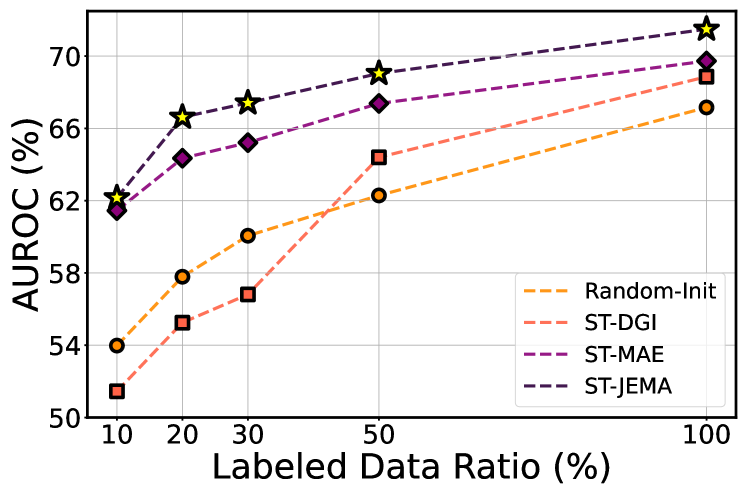
Figure 2: Ablation study on the impact of limited labeled samples for the diagnosis classification task. We fine-tuned the pre-trained GNN model using a limited number of samples, randomly sampled from the ABIDE dataset.

VI-D1 Fine-tuning Performance with Limited Samples

In learning algorithms for analyzing or diagnosing brain disorders with clinical fMRI datasets, a common challenge is the limited number of available training samples. To address this, we aim to enhance model performance in scenarios with limited samples through self-supervised learning. We assessed this by randomly sampling $10\%$, $20\%$, $30\%$, and $50\%$ of the total 884 samples from the ABIDE dataset, and compared the performance with other dynamic graph SSL methods on psychiatric diagnosis classification. As shown in Fig. 2, our proposed ST-JEMA demonstrated superior classification performance even with fewer samples compared to other approaches. Specifically, with the utilization of 20% and 30%, ST-JEMA significantly outperforms other baseline methods. This indicates that the node representations pre-trained with ST-JEMA are more useful for performing downstream tasks, evidencing its potential as a solid pre-trained model for developing more data-efficient models. Notably, ST-DGI fails to outperform Random-Init when utilizing less than 50% of the downstream dataset. This suggests that the pre-trained representation space established through contrastive-based SSL encounters challenges in adapting to the downstream task with a limited number of samples.

VI-D2 Robustness on Missing Data Scenarios

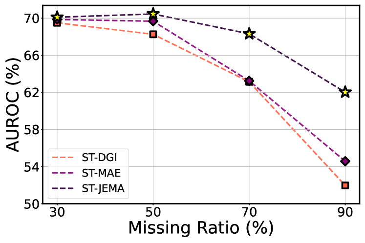
Figure 3: Ablation results on temporal missing data scenarios on psychiatric diagnosis classification task on ABIDE dataset. We designed temporal missing data scenarios by randomly masking the BOLD signal from fMRI data along the time axis, adjusting the missing ratio from 30% to 90%, and then measured the AUROC score to evaluate the effectiveness of SSL in capturing the temporal dynamics.

To further confirm that ST-JEMA successfully captured the temporal dynamics in dynamic FC of fMRI data, we perform ablation experiments on the scenario of temporal missing data for the downstream dataset. Here, the temporal missing data scenario refers to assuming that a certain portion of timesteps is missing from the original data for each sample. To create the missing part from the original downstream training data, we mask randomly selected timesteps in BOLD signal according to a predefined missing ratio. We conduct experiments on the psychiatric diagnosis classification task using the ABIDE dataset, adjusting the missing ratio from 30% to 90%. As demonstrated in Fig. 3, we observed a decline in fine-tuning performance through all methods as the missing ratio increased. This indicates that the loss of temporal flow hinders the accurate prediction of psychiatric disorders, highlighting the importance of learning temporal dynamics for precise predictions. While ST-DGI and ST-MAE exhibited significant performance drops as the missing ratio increased, ST-JEMA maintained relatively better classification performance even with 90% of the data missing along the time axis. This suggests that our proposed SSL method enables the model to effectively learn temporal dynamics, facilitating the learning of pre-trained representations useful for downstream tasks such as psychiatric diagnosis classification.

VI-D3 Ablation on Loss Function

TABLE VI: Ablation results on reconstruction strategies in the loss ${\mathcal{L}}_{\text{ST-JEMA}}$. Here, Baseline (1), (2), (3), and (4) refer to the scenarios where node representation reconstruction, edge reconstruction, spatial, and temporal loss are excluded from ST-JEMA, respectively.

Method Node Edge ${\mathcal{L}}_{spatial}$ ${\mathcal{L}}_{temporal}$ AUROC ($\uparrow$) Random Init ✗ ✗ ✗ ✗ 67.16 Baseline (1) ✗ ✓ ✓ ✓ 68.24 Baseline (2) ✓ ✗ ✓ ✓ 70.33 Baseline (3) ✓ ✓ ✗ ✓ 69.79 Baseline (4) ✓ ✓ ✓ ✗ 65.19 ST-JEMA (Ours) ✓ ✓ ✓ ✓ $\mathbf{71.49}$

In formulating the loss ${\mathcal{L}}_{\text{ST-JEMA}}$ in ST-JEMA, four crucial components are considered: 1) node representation reconstruction loss, 2) edge reconstruction loss, 3) spatial loss, and 4) temporal loss. We perform an ablation study on the construction of the loss function to prove the significance of each component in ${\mathcal{L}}_{\text{ST-JEMA}}$. In this ablation experiment, our target task is the psychiatric diagnosis classification task within the ABIDE dataset. Table VI clearly shows that excluding any loss term from ${\mathcal{L}}_{\text{ST-JEMA}}$ results in a significant drop in performance compared to ST-JEMA. Notably, the most substantial performance decline is observed when excluding the temporal loss ${\mathcal{L}}_{\text{temp}}$, highlighting the critical importance of capturing temporal dynamics in fMRI data for accurately addressing downstream tasks. Meanwhile, the performance of baselines, except when excluding the temporal loss, consistently outperforms the Random Init baseline. This demonstrates the significance of pre-training on a large upstream dataset, particularly in scenarios where the downstream data is limited in terms of labeled samples, as commonly encountered in clinical fMRI datasets. Refer to Appendix Appendix E to see further ablation experiments on the impact of pre-training data size, block mask ratio, and decoder architecture.

VII Conclusion

In this paper, we introduced the Spatio-Temporal Joint-Embedding Masked Autoencoder (ST-JEMA), SSL framework designed for fMRI datasets. Leveraging the recent SSL framework for vision tasks known as JEPA [2], ST-JEMA effectively captures both spatial and temporal dynamics in the dynamic FC of fMRI data by concurrently incorporating two types of reconstruction losses: ${\mathcal{L}}_{\text{spat}}$ and ${\mathcal{L}}_{\text{temp}}$. We empirically validate that ST-JEMA enhances the performance on non-clinical and clinical datasets and three types of tasks compared to competing SSL methods. These findings prove the efficacy of ST-JEMA in fMRI downstream tasks, particularly in scenarios where labeled datasets are limited, which is a common situation in the fMRI research community.

Jungwon Choi is currently working toward a PhD degree at the Kim Jaechul Graduate School of AI, KAIST, Daejeon, Republic of Korea. He received his BS degree in Electronic Engineering from INHA University in 2019, and his MS degree in Electrical Engineering from KAIST in 2021. His current research interests include robust representation learning for real-world scenarios, self-supervised learning, domain generalization, and multi-modal learning on large-scale models.

Hyungi Lee is currently pursuing a PhD degree at the Kim Jaechul Graduate School of AI, KAIST, Daejeon, Republic of Korea. He received his BS degree from the Department of Mathematical Sciences at KAIST in 2020 and his MS degree from the Kim Jaechul Graduate School of AI at KAIST in 2022. His current research interests include neural processes, self-supervised learning, and transfer learning scenarios for large-scale models.

Byung-Hoon Kim is a research assistant professor at the Department of Biomedicine Systems Informatics and Department of Psychiatry, Yonsei University College of Medicine, Seoul, Republic of Korea. He received his PhD degree in Bio & Brain Engineering at KAIST. His primary research focuses on graph representation learning of brain connectivity and its translation to clinical psychiatry.

Juho Lee is an associate professor at the Kim Jaechul Graduate School of AI, KAIST, Daejeon, Republic of Korea. He received his PhD degree in Computer Science & Engineering at POSTECH. He did his postdoc in the Computational Statistics & Machine Learning group at the University of Oxford. His primary research focuses on Bayesian deep learning, Bayesian nonparametric models, meta-learning, and generative models.

Appendix A Algorithmic flow of ST-JEMA

To further facilitate understanding, we summarized the overall pipeline of our proposed Spatio-Temporal Joint Embedding Masked Autoencoder (ST-JEMA) framework for self-supervised learning on fMRI data in Algorithm 1. The algorithm describes the spatial and temporal reconstruction process of node representations and adjacency matrices employing K block masks, assuming the initial conversion of fMRI BOLD signals $\boldsymbol{P}$ into dynamic graphs ${\mathcal{G}}(t)$ has already been completed. Detailed explanations of each equation and the methodological underpinnings can be found in Section IV.

Algorithm 1 Spatio-Temporal Joint Embedding Masked Autoencoder (ST-JEMA)

1:Input: Node features $\boldsymbol{X}(t)$, Adjacency matrix $\boldsymbol{A}(t)$ where $t\in[T_{\mathcal{G}}]$, the number of times for dynamic graphs $T_{\mathcal{G}}$, minimum and maximum masking size ratio of nodes $(\alpha_{\text{min}},\alpha_{\text{max}})$, the number of node N, window length $\Gamma$, window stride $S$, the ratio of spatial reconstruction factor $\gamma$, node reconstruction weight $\lambda_{\texttt{node}}$, and edge reconstruction weight $\lambda_{\texttt{adj}}$.

2:Output: pretrained target GNN encoder $f(\cdot;\bar{\theta})$

3:Initialize context encoder $f_{\texttt{cxt}}$, target encoder $f_{\texttt{tar}}$, node decoder $g_{\texttt{node}}$ and edge decoder $g_{\texttt{edge}}$.

4:for each step do

5:     ${\mathcal{L}}_{\texttt{spat}}\leftarrow 0$ and ${\mathcal{L}}_{\texttt{temp}}\leftarrow 0$ $\triangleright$ Initialize losses for each step

6:     for $t\in{\mathcal{T}}$ do

7:         /* Block masking process.*/

8:         Sample $K$ Block Masks $\boldsymbol{M}_{\boldsymbol{X}}(t),\boldsymbol{M}_{\boldsymbol{A}}(t)$ with $\alpha(t)\sim Uniform(\alpha_{\text{min}},\alpha_{\text{max}})$.

9:         $\boldsymbol{X}_{\texttt{cxt}}(t),\boldsymbol{A}_{\texttt{cxt}}(t)\leftarrow\text{Block Masking}(\boldsymbol{X}(t),\boldsymbol{A}(t),\boldsymbol{M}_{\boldsymbol{X}}(t),\boldsymbol{M}_{\boldsymbol{A}}(t))$

10:         $\boldsymbol{Z}(t)\leftarrow f_{\texttt{cxt}}\Big{(}\boldsymbol{X}_{\texttt{cxt}}(t),\boldsymbol{A}_{\texttt{cxt}}(t);\theta\Big{)}$

11:         $\boldsymbol{Z}_{\texttt{tar}}(t)\leftarrow f_{\texttt{tar}}\Big{(}\boldsymbol{X}(t),\boldsymbol{A}(t);\bar{\theta}\Big{)}$

12:         /* Encode context and target node features */

13:         $\boldsymbol{Z}(t)\leftarrow f_{\texttt{cxt}}\Big{(}\boldsymbol{X}_{\texttt{cxt}}(t),\boldsymbol{A}_{\texttt{cxt}}(t);\theta\Big{)}$

14:         $\boldsymbol{Z}_{\texttt{tar}}(t)\leftarrow f_{\texttt{tar}}\Big{(}\boldsymbol{X}(t),\boldsymbol{A}(t);\bar{\theta}\Big{)}$

15:         /* Spatial reconstruction*/

16:         $\tilde{\boldsymbol{Z}}\leftarrow\boldsymbol{W}_{\texttt{S}}^{{\mathcal{V}}}\boldsymbol{Z}(t)$

17:         $\tilde{\boldsymbol{Z}}_{\texttt{cxt}}(t)\leftarrow\tilde{\boldsymbol{Z}}\odot\Big{(}\boldsymbol{M}_{\boldsymbol{X}}^{(1)}(t)\odot\boldsymbol{M}_{\boldsymbol{X}}^{(2)}(t)\odot\ldots\odot\boldsymbol{M}_{\boldsymbol{X}}^{(K)}(t)\Big{)}$

18:         $\boldsymbol{H}(t)\leftarrow g_{\texttt{edge}}\Big{(}\boldsymbol{W}_{\texttt{S}}^{{\mathcal{E}}}\boldsymbol{Z}(t);\phi_{\mathcal{E}}\Big{)}$

19:         $\hat{\boldsymbol{A}}(t)=\texttt{sig}\Big{(}\boldsymbol{H}(t)\boldsymbol{H}(t)^{\top}\Big{)}$

20:         for $k\in[K]$ do

21:              $\tilde{\boldsymbol{Z}}_{\texttt{cxt}}^{(k)}(t)\leftarrow\tilde{\boldsymbol{Z}}_{\texttt{cxt}}(t)+\boldsymbol{m}\cdot\Big{(}\mathds{1}_{\boldsymbol{X}}-\boldsymbol{M}_{\boldsymbol{X}}^{(k)}(t)\Big{)}$

22:              $\hat{\boldsymbol{Z}}_{\texttt{tar}}^{(k)}(t)\leftarrow g_{\texttt{node}}\Big{(}\tilde{\boldsymbol{Z}}_{\texttt{cxt}}^{(k)}(t);\phi_{\mathcal{V}}\Big{)}$

23:              ${\mathcal{L}}_{\texttt{node-spat}}^{(t)}\leftarrow\frac{1}{K}\sum_{k\in[K]}{\mathcal{L}}_{\texttt{MSE}}\Big{(}\hat{\boldsymbol{Z}}_{\texttt{tar}}^{(k)}(t),\boldsymbol{Z}_{\texttt{tar}}^{(k)}(t)\Big{)}$ $\triangleright$ Spatial node latent reconstruction

24:              ${\mathcal{L}}_{\texttt{adj-spat}}^{(t)}\leftarrow\frac{1}{K}\sum_{k\in[K]}{\mathcal{L}}_{\texttt{BCE}}\Big{(}\hat{\boldsymbol{A}}_{\texttt{tar}}^{(k)}(t),\boldsymbol{A}_{\texttt{tar}}^{(k)}(t)\Big{)}$ $\triangleright$ Spatial adjacency matrix reconstruction

25:         end for

26:         ${\mathcal{L}}_{\texttt{spat}}^{(t)}=\lambda_{\texttt{node}}{\mathcal{L}}_{\texttt{node-spat}}^{(t)}+\lambda_{\texttt{adj}}{\mathcal{L}}_{\texttt{adj-spat}}^{(t)}$

27:         ${\mathcal{L}}_{\texttt{spat}}={\mathcal{L}}_{\texttt{spat}}+{\mathcal{L}}_{\texttt{spat}}^{(t)}$ $\triangleright$ Aggregate spatial reconstruction loss.

28:         /* Temporal reconstruction.*/

29:         Sample $t_{a}\overset{\text{i.i.d.}}{\sim}U_{\text{int}}([0,t-\frac{1}{2}(\frac{\Gamma}{S}+1)]),\quad t_{b}\overset{\text{i.i.d.}}{\sim}U_{\text{int}}([t+\frac{1}{2}(\frac{\Gamma}{S}+1),T_{\mathcal{G}}])$.

30:         $\tilde{\boldsymbol{Z}}_{a,b}(t)\leftarrow\boldsymbol{W}_{\texttt{T}}\Big{[}\tilde{\boldsymbol{Z}}(t_{a})\,\|\,\tilde{\boldsymbol{Z}}(t_{b})\Big{]}$

31:         $\bar{\boldsymbol{A}}_{\texttt{tar}}(t)=\frac{1}{2}\Big{(}\texttt{sig}(\boldsymbol{H}(t_{a})\boldsymbol{H}(t_{b})^{\top})+\texttt{sig}(\boldsymbol{H}(t_{b})\boldsymbol{H}(t_{a})^{\top})\Big{)}$

32:         for $k\in[K]$ do

33:              $\bar{\boldsymbol{Z}}_{\texttt{cxt}}^{(k)}(t)\leftarrow\tilde{\boldsymbol{Z}}_{\texttt{cxt}}(t)+\tilde{\boldsymbol{Z}}_{a,b}(t)\odot\Big{(}\mathds{1}_{\boldsymbol{X}}-\boldsymbol{M}_{\boldsymbol{X}}^{(k)}(t)\Big{)}$

34:              ${\mathcal{L}}_{\texttt{node-temp}}^{(t)}\leftarrow\frac{1}{K}\sum_{k\in[K]}{\mathcal{L}}_{\texttt{MSE}}\Big{(}\bar{\boldsymbol{Z}}_{\texttt{tar}}^{(k)}(t),\boldsymbol{Z}_{\texttt{tar}}^{(k)}(t)\Big{)}$ $\triangleright$ Temporal node latent reconstruction

35:              ${\mathcal{L}}_{\texttt{adj-temp}}^{(t)}=\frac{1}{K}\sum_{k\in[K]}{\mathcal{L}}_{\texttt{BCE}}\Big{(}\bar{\boldsymbol{A}}_{\texttt{tar}}^{(k)}(t),\boldsymbol{A}_{\texttt{tar}}^{(k)}(t)\Big{)}$ $\triangleright$ Temporal adjacency matrix reconstruction

36:         end for

37:         ${\mathcal{L}}_{\texttt{temp}}^{(t)}\leftarrow\lambda_{\texttt{node}}{\mathcal{L}}_{\texttt{node-temp}}^{(t)}+\lambda_{\texttt{adj}}{\mathcal{L}}_{\texttt{adj-temp}}^{(t)}$

38:         ${\mathcal{L}}_{\texttt{temp}}\leftarrow{\mathcal{L}}_{\texttt{temp}}+{\mathcal{L}}_{\texttt{temp}}^{(t)}$$\triangleright$ Aggregate temporal reconstruction loss.

39:     end for

40:     ${\mathcal{L}}_{\texttt{ST-JEMA}}=\gamma{\mathcal{L}}_{\texttt{spat}}+(1-\gamma){\mathcal{L}}_{\texttt{temp}},$

41:     Update ${\theta}$, $\phi_{{\mathcal{V}}}$ and $\phi_{{\mathcal{E}}}$ by taking the gradient descent step with ${\mathcal{L}}_{\texttt{ST-JEMA}}$

42:     Update $\bar{\theta}$ using EMA based on $\theta$.

43:end for

Appendix B Datasets

TABLE VII: Phenotype information summary of the non-clinical and clinical rs-fMRI datasets

Dataset Non-clinical Clinical UKB ABCD HCP-YA HCP-D HCP-A HCP-EP ABIDE ADHD200 COBRE No. Subjects 40913 9111 1093 632 723 176 884 668 173 Gender (F/M) 21682 / 19231 4370 / 4741 594 / 499 339 / 293 405 / 318 67 / 109 138 / 746 242 / 426 43 / 130 Age (Min-Max) 40.0-70.0 8.9-11.0 22.0-37.0 8.1-21.9 36.0-89.8 16.7-35.7 6.47-64.0 7.1-21.8 18.0-66.0 Diagnosis (P/C) - - - - - SPR ASD ADHD BPD / SPR / SZA 120 / 56 408 / 476 280 / 389 (9 / 69 / 11) / 84

B-A Data Preprocessing

We preprocessed all fMRI data to be registered with the standard Montreal Neurological Institute (MNI) space, ensuring consistency and comparability across datasets. The region of interest (ROI)-time-series matrices were extracted using the Schaefer atlas [21], which identifies 400 distinct ROIs within the brain for analyzing functional connectivity.

From the time-series BOLD signal $\boldsymbol{P}$ in each fMRI dataset, we construct two types of graphs: a static graph and a dynamic graph. While the dynamic graph is constructed as described in Section III-C, for the static graph, we build the adjacency matrix $\boldsymbol{A}$ to represent the functional connectivity of ROI by windowing across all time stamps $\tau\in[T_{max}]$. Additionally, the node feature $\boldsymbol{X}$ is constructed using one-hot positional encoding, followed by a projection through the matrix $\boldsymbol{W}$.

B-B Data Description

UK Biobank (UKB) [23]: We utilized 40,913 samples of resting-state fMRI from the UK Biobank, a comprehensive biomedical database of genetic, lifestyle, and health information from half a million participants. This dataset supports advanced medical research by offering insights into serious illnesses through diverse data collections, including genome sequencing, health record linkages, and functional MRI imaging.

Adolescent Brain Cognitive Development (ABCD) [4]: A longitudinal study tracking nearly 12,000 youth across 21 research sites to investigate the impact of childhood experiences on brain development and various behavioral, social, and health outcomes. We constructed 9,111 samples aged 9 to 11 years.

Human Connectome Project Young Adults (HCP-YA) [26]: Mapping the connectome of healthy individuals, this project provides a comprehensive database from 1,200 young adults, incorporating advanced 3T and 7T MRI scanners for an exploration of brain connectivity and function. In our study, we specifically utilized rs-fMRI data from 1,093 subjects, following the pre-processing methodology described in Kim et al. [12].

Human Connectome Project Aging (HCP-A) [2]: Investigating the effects of aging on brain structure and function, this segment of the Human Connectome Project includes 1200 adults aged 36 to 100+ years. It aims to uncover how brain connections change with age in healthy individuals using a 3T MRI scanner. For our analysis, we utilized rs-fMRI data from 724 samples aged 36 to 89 years.

Human Connectome Project Development (HCP-D) [22]: This dataset includes over 1,300 participants ranging from 5 to 21 years old, exploring the dynamics of brain development from childhood through adolescence using a 3T MRI scanner. Specifically, our study utilizes rs-fMRI data from 632 individuals aged between 8 and 21 years.

Human Connectome Project for Early Psychosis (HCP-EP) [17]: Focusing on early psychosis within the first three years of symptom onset, this dataset includes comprehensive imaging using a 3T MRI scanner, behavioral, clinical, cognitive, and genetic data from 400 subjects aged 16 to 35 years, including labels for schizophrenia (SPR). The objective is to identify disruptions in neural connections that underlie both brain function and dysfunction during a critical period with fewer confounds such as prolonged medication exposure. Our study employs rs-fMRI data from 176 subjects.

Autism Brain Imaging Data Exchange (ABIDE) [6]: This dataset gathers rs-fMRI, anatomical, and phenotypic data from 1,112 individuals across 17 international sites, aiming to enhance the understanding of Autism Spectrum Disorder (ASD) through collaborative research. For our study, we specifically utilized rs-fMRI data from 884 individuals, ranging in age from 6 to 64 years.

ADHD200 [3]: This dataset initiative advances Attention Deficit Hyperactivity Disorder (ADHD) research by offering unrestricted access to 776 resting-state fMRI and anatomical datasets of individuals aged from 7 to 21 years, which includes 285 subjects with ADHD and 491 typically developing controls, from 8 international imaging sites. In our study, we utilized rs-fMRI data from 668 subjects.

The Center for Biomedical Research Excellence (COBRE)) [18] : We constructed rs-fMRI datasets comprising 173 samples, including 84 patients with schizophrenia (SPR), 9 with bipolar disorder (BPD), 11 with schizoaffective disorder (SZA), and 75 healthy controls, ranging in age from 18 to 66 years. This dataset aims to facilitate the exploration of neural mechanisms underlying various mental illnesses.

Appendix C Competing Methods

To compare with our proposed ST-JEMA, we evaluated eight competing algorithms, each designed for pre-training GNN encoders using SSL methods, excluding Random-Init:

Random-Init: Training from scratch on the downstream dataset without the pre-training step using the upstream dataset. We present two sets of results for Random-Init, specifically when using a static graph as input and a dynamic graph as input, as elaborated in Section B-A.

DGI [25]: A contrastive SSL method for static graph data that learns mutual information between node and graph representations.

SimGRACE [27]: A contrastive SSL method for static graph data that utilizes model parameter perturbation to generate different views instead of using graph augmentations.

GAE [15]: A generative SSL method for static graph data that utilizes an autoencoder framework. GAE reconstructs a graph’s original adjacency matrix by leveraging node representations.

VGAE [15]: A generative SSL method for static graph data that improves GAE by using a variational autoencoder in the encoder.

GraphMAE [9]: A generative SSL method for static graph data that focuses on node reconstruction with masked autoencoder loss.

ST-DGI [19]: A contrastive SSL method for dynamic graph data that enhances DGI by optimizing the mutual information between node embeddings $\boldsymbol{Z}(t)$ and features at future k-time steps $\boldsymbol{Z}(t+k)$.

ST-MAE [5]: A generative SSL method specifically designed for fMRI data. ST-MAE focuses on dynamic FC by utilizing a masked autoencoder framework that accounts for temporal dynamics.

Appendix D Experimental Details

In this section, we detail the implementation of the models for ST-JEMA and training pipelines for upstream and downstream datasets.

D-A Architecture Details

In this research, we utilize a 4-layer Graph Isomorphism Network (GIN) [28] as the GNN encoder and the Squeeze-Excitation READOUT (SERO) readout module in the fine-tuning process following the approach introduced by Kim et al. [12]. To ensure that each decoder effectively reconstructs target components from context node representations, we employ MLP-Mixer [24] for both node and edge decoders. Here, we provide detailed architectural information about GIN, SERO, and MLP-Mixer.

Graph Isomorphism Network (GIN) [28]:

Graph Isomorphism Networks, are specialized spatial GNN optimized for graph classification, achieving performance comparable to the Weisfeiler-Lehman (WL) test [16]. The GIN architecture aggregates neighboring node features through summation and employs an MLP for feature transformation, enabling the learning of injective mappings. This unique structure enables GINs to adeptly capture complex graph patterns, proving particularly effective in analyzing fMRI data for tasks such as gender classification from rs-fMRI data [13]. The mathematical formulation of GIN at layer $l$ is as follows:

$$\boldsymbol{z}_{i}^{(l)}=\text{MLP}^{(l)}\left((1+\epsilon^{(l)})\cdot\boldsymbol{z}_{i}^{(l-1)}+\sum_{j\in{\mathcal{N}}(i)}\boldsymbol{z}_{j}^{(l-1)}\right),$$ (38)

where $\epsilon^{(k)}$ is a parameter optimized during training. The application of GINs to fMRI data analysis marks a significant progression, offering refined insights into the spatial and temporal dynamics of brain activity.

Squeeze-Excitation READOUT (SERO) [12]: SERO is the noble readout module that adapts the concept of attention mechanisms from Squeeze-and-Excitation Networks [10], adjusting it to apply attention across the node dimension instead of the channel dimension for GNNs. This modification enhances the focus on the structural and functional properties of nodes within brain graphs. The attention mechanism is mathematically defined as follows:

$$\boldsymbol{a}_{\text{space}}(t)=\texttt{sig}\big{(}\boldsymbol{W}_{2}\sigma(\boldsymbol{W}_{1}\boldsymbol{Z}(t)\Phi_{\text{mean}})\big{)},$$ (39)

where $\Phi_{\text{mean}}=[1/N,...,1/N]$ is a mean vector for mean pooling, $\boldsymbol{W}_{1}\in\mathbb{R}^{d_{\text{enc}}\times d_{\text{enc}}},\boldsymbol{W}_{2}\in\mathbb{R}^{N\times d_{\text{enc}}}$ are learnable parameter matrices, and $\sigma$ is the nonlinear activation function such as ReLU. Finally, The graph representation at time $t$ is derived by applying attention weights $\boldsymbol{a}_{\text{space}}$(t) to each node of $Z(t)$, effectively weighting the importance of each node’s features in the overall graph representation as follows:

$$\boldsymbol{z}_{G}(t)=\boldsymbol{Z}(t)\boldsymbol{a}_{\text{space}}(t).$$ (40)

This readout $\boldsymbol{z}_{G}(t)$ is used when the model is fine-tuned on the downstream task. When integrated into the STAGIN [12] framework, this module significantly enhances performance in gender and task classification on fMRI data, demonstrating advancements over existing models.

MLP-Mixer [24]: MLP-Mixer adopts a purely MLP-based architecture, diverging from conventional convolution and self-attention mechanisms, comprising of token-mixing and channel-mixing Multi-Layer Perceptrons (MLPs). In this setup, we utilize the token-mixing MLPs to encourage interactions among nodes, while the channel-mixing MLPs facilitates feature communication across the feature dimension of node representations. For a graph with node representations $\mathbf{Z}\in\mathbb{R}^{N\times D}$, where $N$ is the number of nodes and $D$ is the dimension of node features, the MLP-Mixer operates as follows:

$$\begin{gathered}\boldsymbol{Y}_{*,i}=\boldsymbol{Z}_{*,i}+\boldsymbol{W}_{2}\texttt{GELU}(\boldsymbol{W}_{1}\texttt{LN}(\boldsymbol{Z})_{*,i}),\,i=\{1,...,N\},\\ \hat{\boldsymbol{Z}}_{j,*}=\boldsymbol{Y}_{j,*}+\boldsymbol{W}_{4}\texttt{GELU}(\boldsymbol{W}_{3}\texttt{LN}(\boldsymbol{Y})_{j,*}),\,j=\{1,...,D\},\end{gathered}$$ (43)

where GELU [8] is a non-linear activation function and LN [1] is a layer normalization. And $\boldsymbol{W}_{1}\in\mathbb{R}^{\bar{N}\times N}$, $\boldsymbol{W}_{2}\in\mathbb{R}^{N\times\bar{N}}$, $\boldsymbol{W}_{3}\in\mathbb{R}^{\bar{D}\times D}$, and $\boldsymbol{W}_{4}\in\mathbb{R}^{D\times\bar{D}}$ are learnable parameters for each MLPs with hidden dimension of $\bar{N}$ and $\bar{D}$. This adaptation allows the MLP-Mixer to ensure communication between nodes for the reconstruction of targeted node representations from the aggregated context of the graph.

D-B Hyperparameter Details

In this study, we optimize GNN encoder in two phases: 1) pretraining the GNN encoder using SSL method on the upstream dataset, 2) finetuning the GNN encoder for classification or regression tasks on the downstream dataset.

For the upstream dataset in our SSL methods, we utilize the UKB dataset with a window size $\Gamma=50$ and a window stride $S=16$ for constructing dynamic graphs. We split the upstream dataset into train (80%) / validation (10%) / test (10%) partitions and selected the pre-trained model for each SSL method based on the best-performing upstream SSL task on the test dataset. For downstream tasks, we construct dynamic graphs from fMRI datasets such as ABCD, HCP-YA, HCP-A, HCP-D, and HCP-EP are processed with a window size of 50 and a stride of 16. For the ABIDE, ADHD200, and COBRE datasets, we use a window size of 16 and a stride of 3 for consistency of fMRI scanning time. Following the approach by Kim et al. [12], we also randomly sliced the time dimension of the ROI-time-series BOLD signal matrix $\boldsymbol{P}$, setting dynamic lengths of 400 for UKB, HCP-A, HCP-D, and HCP-EP; 380 for ABCD; 600 for HCP-YA; 70 for ABIDE and ADHD200; and 120 for COBRE.

Optimization hyperparameters include a learning rate of $1\times 10^{-4}$ for ST-DGI, $5\times 10^{-4}$ for ST-MAE, and $5\times 10^{-5}$ for other SSL methods, with a consistent weight decay of $1\times 10^{-4}$ in the pre-training phase. For finetuning, a learning rate of $5\times 10^{-4}$ is used for gender and psychiatric diagnosis classification tasks, and $1\times 10^{-3}$ for the age regression task, selecting the best-performing model within weight decays of $\{1\times 10^{-3},5\times 10^{-4},1\times 10^{-4}\}$. For Random-Init, a learning rate of $1\times 10^{-3}$ and weight decay of $1\times 10^{-4}$ are used across all tasks.

Additional hyperparameters for each SSL method are summarized as follows:

• SimGRACE: Perturbation scale $\eta=1.0$.

• GraphMAE: Random masking ratio $\alpha\,(\%)=\{30,50,70\}$.

• ST-DGI: $k=\{1,3,6\}$.

• ST-MAE: Random masking ratio $\alpha\,(\%)=\{30,50,70\}$.

• ST-JEMA: Block masking ratio $[\alpha_{\min},\alpha_{\max}]\,(\%)=\{10\text{-}15,15\text{-}20,20\text{-}25,25\text{-}30\}$, $\gamma=0.5$, $\lambda_{\text{node}}=1.0$, $\lambda_{\text{edge}}=\{1\times 10^{-3},1\times 10^{-4},1\times 10^{-5},1\times 10^{-6}\}$.

Appendix E Additional Ablation Studies

We conduct additional ablation studies to evaluate the impact of SSL data size, the optimal block mask ratio., and assess the feasibility of the proposed decoder architecture.

E-A Impact of Pre-Training Data Size

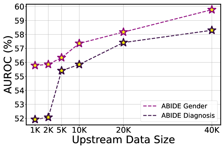
Figure 4: Ablation study on the impact of sample size for SSL on the ABIDE dataset. We evaluated learned representations for downstream tasks by training a linear probing model across varying numbers of samples.

To confirm the impact of the quantity of upstream UKB data on the quality of the pre-trained representation by the GNN encoder, we perform an ablation experiment by varying the size of the pre-training data. To systematically evaluate the impact of varying training data sizes on the effectiveness of pre-trained representations in solving downstream tasks, we conducted linear probing on the gender classification task and the diagnosis classification task using the ABIDE dataset. Notably, linear probing preserves the pre-trained representations even after the fine-tuning process which effectively shows the quality of pre-trained representations. Fig. 4 clearly indicates that the performance improves as the size of the training data increases. This result demonstrates that ST-JEMA successfully learns more meaningful representations as the training dataset size increases. It suggests that ST-JEMA is adept at acquiring high-quality representations from the extensive UKB upstream dataset.

E-B Ablation on Block Mask Ratio

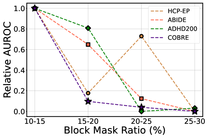
Figure 5: Ablation study on the block mask ratio of ST-JEMA for psychiatric diagnosis classification in clinical data. The x-axis, representing the block mask ratio, signifies the relative ratio of the minimum and maximum values within a specified range relative to the total size. The size of each block mask is randomly sampled from this range. To provide the outcomes across all datasets simultaneously, we present the relative AUROC results. Here, we calculate the relative AUROC by normalizing using the minimum and maximum AUROC results obtained from different block mask ratio ranges.

In the masking process of target points in ST-JEMA, selecting the appropriate block mask ratio is crucial. It is essential to strike a balance that ensures sufficient information for reconstructing the target representation, while also making the problem challenging enough to prevent the GNN encoder from learning trivial representations. To analyze the appropriate block mask ratio in ST-JEMA, we perform an ablation experiment on the block mask ratio using the diagnosis classification task.

In Fig. 5, one can see that utilizing $10\%\sim 15\%$ is the optimal block mask ratio across all datasets. The trends are consistent across all datasets except for HCP-EP, where the performance improves with a block mask ratio of $20\%\sim 25\%$ compared to $15\%\sim 20\%$. Since we employ $4$ masks for each timestep $t\in[T_{{\mathcal{G}}}]$, the optimal block mask ratio might change if the number of masks per each node and adjacency matrix is altered.

E-C Decoder Architecture

TABLE VIII: Ablation results on different architecture for decoder module with diagnosis classification task on ABIDE dataset. The performance is evaluated using the AUROC score, with higher scores indicating better performance.

Decoder architecture	AUROC ($\uparrow$)
MLP	64.76
GIN [28]	66.35
MLP-Mixer [24]	$\mathbf{71.49}$

As described in Section IV, We implemented the MLP-Mixer [24] to reconstruct the target node representation by integrating information from context node representations. Another approach to aggregate representations from different nodes is by using a GNN decoder. GraphMAE employed a more expressive GNN decoder instead of a simple MLP to prevent learning representations nearly identical to the low-level semantics of input features, thus aiming to capture higher-level semantics.

To determine which decoder structure is most effective for our methodology, we compared an MLP module, a one-layer GIN module, and a one-layer MLP-Mixer module. The MLP module does not utilize information from other node representations for reconstructing the target node and hence does not use a learnable token for node representation; instead, it reconstructs the target node representation using the corresponding node representation obtained from the GNN encoder. As seen in Table VIII, the MLP decoder exhibited the lowest performance, possibly due to the pre-trained representations being of low-level semantics. While the GIN module performed better, its performance was similar to that of a random initialization, indicating limited benefit. In contrast, our method using the MLP-Mixer facilitated interactions among context node representations, thereby learning representations with higher-level semantics.

Appendix F Additional Related Works

F-A Contrastive Self-supervised Learning on Graph

Contrastive methods focus on aligning representations derived from different ‘views’ of input graphs, known as positive pairs, typically generated through data augmentations or multiple snapshots of the same graph. The primary goal is to maximize the agreement between these positive pairs of samples, thereby enhancing the model’s ability to capture meaningful relationships within the data. To achieve this, a projection head is commonly employed to transform the encoder’s representations into an optimized feature space, enhancing discriminative power and learning stability while mitigating overfitting and preventing representation mode collapse [11, 7]. DGI [25] pioneered in graph contrastive SSL, aiming to maximize the mutual information between local and global graph representations. Subsequently, GraphCL [29] introduced graph augmentations to create different views for contrastive learning. However, the effectiveness of these augmentations can vary across different domains and sometimes restrict the graph structure. In response to these challenges, alternative strategies have been developed to bypass the need for complex augmentations. SimGCL [30] adopted a novel approach by adding noise to the embedding space to generate contrastive views, while SimGRACE [27] simplified the process by leveraging correlated views from perturbed GNN parameters.

F-B Generative Self-supervised Learning on Graph

Generative approaches aim to reconstruct the original input by leveraging the encoded representations. Employing a decoder, these methods are tasked with reconstructing the original graph structure from the encoder’s embeddings. By optimizing the GNN model for precise reconstruction of the graph structure, generative methods enable the learning of representations that inherently capture the structural relationships in graph data. VGAE [15], a pioneer work in generative approach, introduces strategies to reconstruct a graph’s adjacency matrix from node embeddings. Utilizing variational autoencoders [14], VGAE demonstrates better performance in link prediction than conventional unsupervised learning methods. DeepWalk [20], highlighting their effectiveness in identifying important patterns in graph-structured data without labeled graph data. GraphMAE [9] adopts a novel approach to SSL in graph data by implementing a masked autoencoder for node feature reconstruction. GraphMAE demonstrates notable advantages over traditional contrastive learning techniques in tasks such as node and graph classification, showing evidence that generative self-supervised is also effective in the graph domain beyond the computer vision task.

References

- [1] (2016) Understanding intermediate layers using linear classifier probes. arXiv preprint arXiv:1610.01644. Cited by: §VI-B.
- [2] (2023) Self-supervised learning from images with a joint-embedding predictive architecture. In Proceedings of the IEEE/CVF Conference on Computer Vision and Pattern Recognition, pp. 15619–15629. Cited by: §I, §II-C, §III-D, §IV-A, §IV-B, §IV-C, §VII.
- [3] (2019) The lifespan human connectome project in aging: an overview. Neuroimage 185, pp. 335–348. Cited by: §V.
- [4] (2012) ADHD-200 global competition: diagnosing adhd using personal characteristic data can outperform resting state fmri measurements. Frontiers in systems neuroscience 6, pp. 69. Cited by: §V.
- [5] (2018) The adolescent brain cognitive development (abcd) study: imaging acquisition across 21 sites. Developmental cognitive neuroscience 32, pp. 43–54. Cited by: §V.
- [6] (2021) An empirical study of training self-supervised vision transformers. in 2021 ieee. In CVF International Conference on Computer Vision (ICCV), pp. 9620–9629. Cited by: §I.
- [7] (2023) A generative self-supervised framework using functional connectivity in fmri data. In Temporal Graph Learning Workshop@ NeurIPS 2023, Cited by: §I, §I, §II-B, §IV-D, §IV-D, §V.
- [8] (2014) Empirical evaluation of gated recurrent neural networks on sequence modeling. arXiv preprint arXiv:1412.3555. Cited by: §III-C.
- [9] (2013) The neuro bureau preprocessing initiative: open sharing of preprocessed neuroimaging data and derivatives. Frontiers in Neuroinformatics 7 (27), pp. 5. Cited by: §V.
- [10] (2018) Bert: pre-training of deep bidirectional transformers for language understanding. arXiv preprint arXiv:1810.04805. Cited by: §I.
- [11] (2020) Spatio-temporal graph convolution for resting-state fmri analysis. In Medical Image Computing and Computer Assisted Intervention–MICCAI 2020: 23rd International Conference, Lima, Peru, October 4–8, 2020, Proceedings, Part VII 23, pp. 528–538. Cited by: §I, §II-B.
- [12] (2020) Bootstrap your own latent-a new approach to self-supervised learning. Advances in neural information processing systems 33, pp. 21271–21284. Cited by: §IV-A.
- [13] (2022) Masked autoencoders are scalable vision learners. In Proceedings of the IEEE/CVF conference on computer vision and pattern recognition, pp. 16000–16009. Cited by: §I, §II-C.
- [14] (2022) Graphmae: self-supervised masked graph autoencoders. In Proceedings of the 28th ACM SIGKDD Conference on Knowledge Discovery and Data Mining, pp. 594–604. Cited by: §I, §I, §I, §II-B, §IV-C, §V.
- [15] (2022) Fbnetgen: task-aware gnn-based fmri analysis via functional brain network generation. In International Conference on Medical Imaging with Deep Learning, pp. 618–637. Cited by: §II-A.
- [16] (2018) 3D convolutional neural networks for classification of functional connectomes. In International Workshop on Deep Learning in Medical Image Analysis, pp. 137–145. Cited by: §I.
- [17] (2021) Learning dynamic graph representation of brain connectome with spatio-temporal attention. Advances in Neural Information Processing Systems 34, pp. 4314–4327. Cited by: §I, §II-A, §III-B, §IV-B, §V.
- [18] (2020) Understanding graph isomorphism network for rs-fmri functional connectivity analysis. Frontiers in neuroscience 14, pp. 630. Cited by: §I.
- [19] (2016) Variational graph auto-encoders. arXiv preprint arXiv:1611.07308. Cited by: §II-B, §IV-C, §V.
- [20] (2020) Neuroprogression across the early course of psychosis. Journal of psychiatry and brain science 5. Cited by: §V.
- [21] (2021) Braingnn: interpretable brain graph neural network for fmri analysis. Medical Image Analysis 74, pp. 102233. Cited by: §II-A.
- [22] (2023) BrainTGL: a dynamic graph representation learning model for brain network analysis. Computers in Biology and Medicine 153, pp. 106521. Cited by: §II-A.
- [23] (2013) Functional imaging of the hemodynamic sensory gating response in schizophrenia. Human brain mapping 34 (9), pp. 2302–2312. Cited by: §V.
- [24] (2019) Spatio-temporal deep graph infomax. arXiv preprint arXiv:1904.06316. Cited by: §V.
- [25] (2018) Local-global parcellation of the human cerebral cortex from intrinsic functional connectivity mri. Cerebral cortex 28 (9), pp. 3095–3114. Cited by: §III-C.
- [26] (2018) The lifespan human connectome project in development: a large-scale study of brain connectivity development in 5–21 year olds. Neuroimage 183, pp. 456–468. Cited by: §V.
- [27] (2015) UK biobank: an open access resource for identifying the causes of a wide range of complex diseases of middle and old age. PLoS medicine 12 (3), pp. e1001779. Cited by: §V.
- [28] (2022) Mgae: masked autoencoders for self-supervised learning on graphs. arXiv preprint arXiv:2201.02534. Cited by: §IV-C.
- [29] (2021) Mlp-mixer: an all-mlp architecture for vision. Advances in neural information processing systems 34, pp. 24261–24272. Cited by: §IV-C.
- [30] (2018) Deep graph infomax. arXiv preprint arXiv:1809.10341. Cited by: §II-B, §V.
- [31] (2021) Modeling dynamic characteristics of brain functional connectivity networks using resting-state functional mri. Medical image analysis 71, pp. 102063. Cited by: §II-A.
- [32] (2022) Masked feature prediction for self-supervised visual pre-training. In Proceedings of the IEEE/CVF Conference on Computer Vision and Pattern Recognition, pp. 14668–14678. Cited by: §I.
- [33] (2017) 1200 subjects data release reference manual. URL https://www. humanconnectome. org 565. Cited by: §V.
- [34] (2022) Simgrace: a simple framework for graph contrastive learning without data augmentation. In Proceedings of the ACM Web Conference 2022, pp. 1070–1079. Cited by: §I, §II-B, §V.
- [35] (2019) How powerful are graph neural networks?. International Conference on Learning Representations. Cited by: §V.
- [36] (2019) Groupinn: grouping-based interpretable neural network for classification of limited, noisy brain data. In Proceedings of the 25th ACM SIGKDD international conference on knowledge discovery & data mining, pp. 772–782. Cited by: §II-A.
- [37] (2019) Functional connectivity magnetic resonance imaging classification of autism spectrum disorder using the multisite abide dataset. In 2019 IEEE EMBS International Conference on Biomedical & Health Informatics (BHI), pp. 1–4. Cited by: §I.
- [38] (2020) Graph contrastive learning with augmentations. Advances in neural information processing systems 33, pp. 5812–5823. Cited by: §I, §II-B.
- [39] (2022) Are graph augmentations necessary? simple graph contrastive learning for recommendation. In Proceedings of the 45th international ACM SIGIR conference on research and development in information retrieval, pp. 1294–1303. Cited by: §II-B.

References

- [1] (2016) Layer normalization. arXiv preprint arXiv:1607.06450. Cited by: §D-A.
- [2] (2019) The lifespan human connectome project in aging: an overview. Neuroimage 185, pp. 335–348. Cited by: §B-B.
- [3] (2012) ADHD-200 global competition: diagnosing adhd using personal characteristic data can outperform resting state fmri measurements. Frontiers in systems neuroscience 6, pp. 69. Cited by: §B-B.
- [4] (2018) The adolescent brain cognitive development (abcd) study: imaging acquisition across 21 sites. Developmental cognitive neuroscience 32, pp. 43–54. Cited by: §B-B.
- [5] (2023) A generative self-supervised framework using functional connectivity in fmri data. In Temporal Graph Learning Workshop@ NeurIPS 2023, Cited by: Appendix C.
- [6] (2013) The neuro bureau preprocessing initiative: open sharing of preprocessed neuroimaging data and derivatives. Frontiers in Neuroinformatics 7 (27), pp. 5. Cited by: §B-B.
- [7] (2022) Understanding and improving the role of projection head in self-supervised learning. arXiv preprint arXiv:2212.11491. Cited by: §F-A.
- [8] (2016) Gaussian error linear units (gelus). arXiv preprint arXiv:1606.08415. Cited by: §D-A.
- [9] (2022) Graphmae: self-supervised masked graph autoencoders. In Proceedings of the 28th ACM SIGKDD Conference on Knowledge Discovery and Data Mining, pp. 594–604. Cited by: Appendix C, §F-B.
- [10] (2018) Squeeze-and-excitation networks. In Proceedings of the IEEE conference on computer vision and pattern recognition, pp. 7132–7141. Cited by: §D-A.
- [11] (2021) Understanding dimensional collapse in contrastive self-supervised learning. International Conference on Learning Representations. Cited by: §F-A.
- [12] (2021) Learning dynamic graph representation of brain connectome with spatio-temporal attention. Advances in Neural Information Processing Systems 34, pp. 4314–4327. Cited by: §B-B, §D-A, §D-A, §D-A, §D-B.
- [13] (2020) Understanding graph isomorphism network for rs-fmri functional connectivity analysis. Frontiers in neuroscience 14, pp. 630. Cited by: §D-A.
- [14] (2013) Auto-encoding variational bayes. arXiv preprint arXiv:1312.6114. Cited by: §F-B.
- [15] (2016) Variational graph auto-encoders. arXiv preprint arXiv:1611.07308. Cited by: Appendix C, Appendix C, §F-B.
- [16] (1968) A reduction of a graph to a canonical form and an algebra arising during this reduction. Nauchno-Technicheskaya Informatsiya 2 (9), pp. 12–16. Cited by: §D-A.
- [17] (2020) Neuroprogression across the early course of psychosis. Journal of psychiatry and brain science 5. Cited by: §B-B.
- [18] (2013) Functional imaging of the hemodynamic sensory gating response in schizophrenia. Human brain mapping 34 (9), pp. 2302–2312. Cited by: §B-B.
- [19] (2019) Spatio-temporal deep graph infomax. arXiv preprint arXiv:1904.06316. Cited by: Appendix C.
- [20] (2014) Deepwalk: online learning of social representations. In Proceedings of the 20th ACM SIGKDD international conference on Knowledge discovery and data mining, pp. 701–710. Cited by: §F-B.
- [21] (2018) Local-global parcellation of the human cerebral cortex from intrinsic functional connectivity mri. Cerebral cortex 28 (9), pp. 3095–3114. Cited by: §B-A.
- [22] (2018) The lifespan human connectome project in development: a large-scale study of brain connectivity development in 5–21 year olds. Neuroimage 183, pp. 456–468. Cited by: §B-B.
- [23] (2015) UK biobank: an open access resource for identifying the causes of a wide range of complex diseases of middle and old age. PLoS medicine 12 (3), pp. e1001779. Cited by: §B-B.
- [24] (2021) Mlp-mixer: an all-mlp architecture for vision. Advances in neural information processing systems 34, pp. 24261–24272. Cited by: §D-A, §D-A, §E-C, TABLE VIII.
- [25] (2018) Deep graph infomax. arXiv preprint arXiv:1809.10341. Cited by: Appendix C, §F-A.
- [26] (2017) 1200 subjects data release reference manual. URL https://www. humanconnectome. org 565. Cited by: §B-B.
- [27] (2022) Simgrace: a simple framework for graph contrastive learning without data augmentation. In Proceedings of the ACM Web Conference 2022, pp. 1070–1079. Cited by: Appendix C, §F-A.
- [28] (2019) How powerful are graph neural networks?. International Conference on Learning Representations. Cited by: §D-A, §D-A, TABLE VIII.
- [29] (2020) Graph contrastive learning with augmentations. Advances in neural information processing systems 33, pp. 5812–5823. Cited by: §F-A.
- [30] (2022) Are graph augmentations necessary? simple graph contrastive learning for recommendation. In Proceedings of the 45th international ACM SIGIR conference on research and development in information retrieval, pp. 1294–1303. Cited by: §F-A.