LiDAR Point Cloud-based Multiple Vehicle Tracking with Probabilistic Measurement-Region Association

Abstract

Multiple extended target tracking (ETT) has gained increasing attention due to the development of high-precision LiDAR and radar sensors in automotive applications. For LiDAR point cloud-based vehicle tracking, this paper presents a probabilistic measurement-region association (PMRA) ETT model, which can describe the complex measurement distribution by partitioning the target extent into different regions. The PMRA model overcomes the drawbacks of previous data-region association (DRA) models by eliminating the approximation error of constrained estimation and using continuous integrals to more reliably calculate the association probabilities. Furthermore, the PMRA model is integrated with the Poisson multi-Bernoulli mixture (PMBM) filter for tracking multiple vehicles. Simulation results illustrate the superior estimation accuracy of the proposed PMRA-PMBM filter in terms of both positions and extents of the vehicles comparing with PMBM filters using the gamma Gaussian inverse Wishart and DRA implementations.

I Introduction

LiDAR and radar point clouds can provide abundant and accurate spatial information of the surrounding environment, which is vital for perception tasks such as target detection and tracking in autonomous driving and intelligent transportation systems [1, 2, 3, 4, 5]. In the context of point cloud-based multiple target tracking (MTT), extended target tracking (ETT) methods have attracted increasing attentions [6, 7, 8]. The ETT differs from traditional MTT approaches by assuming the sensor can gather multiple measurements of a target in each scan, thus allowing for the simultaneous estimation of the target’s location and extent directly from the point cloud [9, 10].

The modeling of extended targets significantly affects the performance of ETT as it determines the spatial distribution of target measurements. For instance, the gamma Gaussian inverse Wishart (GGIW) random matrix model [11] assumes measurements are Gaussian distributed around the target’s center; the random hypersurface model (RHM) [12] assumes the measurement sources are uniformly distributed on a star-convex shaped target extent. For LiDAR-based ETT, these widely accepted models are inaccurate and could degrade the tracking performance because the point clouds often congregate on the target’s contour rather than spreading across the entire surface [9]. Recently, several ETT methods based on data-region association (DRA) are developed for tracking single vehicle with automotive radar [14, 13]. The DRA methods depict the complex distribution of radar point clouds with a simple and intuitive model, where the rectangular vehicle extent is partitioned into four edges and an interior area. Different regions are associated with measurements and the estimates from all regions are combined into the tracking result based on association probabilities. The effectiveness of DRA has been evaluated by both simulated and real data. However, these methods rely on constrained estimation to obtain rectangular extents, which introduces complexity and approximation errors. Besides, the data-region association probabilities are calculated with randomly distributed scattering centers, thus further reducing the robustness of the algorithm.

The objective of this study is to overcome the deficiencies of DRA methods and extend the region-partitioning idea to LiDAR point cloud-based multiple vehicle tracking. To this end, we design the probabilistic measurement-region association (PMRA) model, which can directly obtain rectangular extents using the Wishart distribution. The PMRA model also utilizes continuous integrals and the visible angle of regions to improve the accuracy and stability for calculating the association probabilities. For tracking multiple vehicles, we integrate the PMRA model with the Poisson multi-Bernoulli mixture (PMBM) filter, a state-of-the-art MTT framework [15, 16]. Simulation results show that the PMRA-PMBM filter with its particle implementation achieves higher estimation accuracy in terms of both positions and extents of the vehicles compared to GGIW and DRA implementations of the PMBM filter.

II System Modeling

A system model based on random finite set (RFS) and PMBM conjugate prior is applied in this study. At time step $k$, the multi-target state is represented by an RFS $\mathbf{X}_{k}=\{\mathbf{x}_{k}^{i}\}_{i\in\mathbf{I}_{k}}$ where $\mathbf{I}_{k}$ is the target index set with cardinality $|\mathbf{I}_{k}|=N_{k}$; both the single target state $\mathbf{x}_{k}^{i}$ and number of targets $N_{k}$ are random. Similarly, the set of measurements is expressed as $\mathbf{Z}_{k}=\{\mathbf{z}_{k}^{m}\}_{m\in\mathbf{M}_{k}}$ with $|\mathbf{M}_{k}|=M_{k}$, and the collection of all measurement sets from time $1$ to time $k$ is denoted by $\mathbf{Z}^{k}$. For LiDAR-based ETT, the 3D point cloud is usually projected to the 2D bird’s-eye-view (BEV) plane before tracking [6, 7]. In this work, we follow the same approach and define the system model on the global Cartesian coordinate system, as illustrated in Fig. 1.

Figure 1: Illustration of the system model. $(x_{\mathrm{s}},y_{\mathrm{s}})$ and $(x_{\mathrm{t}},y_{\mathrm{t}})$ denote the positions of LiDAR and target. The target extent is divided into five regions $r_{1}$-$r_{5}$. The vertices $\mathbf{p}^{1}$-$\mathbf{p}^{4}$ are determined by the eigenvectors $\{\mathbf{e}^{1},\mathbf{e}^{2}\}$ and eigenvalues $\{e^{1},e^{2}\}$ of the extent matrix $E$.

II-A RFSs and PMBM Posterior Density

The RFSs used in our system modeling are briefly introduced in this section. A Poisson point process (PPP) is an RFS with Poisson distributed cardinality and i.i.d. elements. Thus, the density of PPP RFS is defined by

$$f^{\mathrm{ppp}}(\mathbf{X})=e^{-\mu}\prod_{\mathbf{x}\in\mathbf{X}}\mu f(\mathbf{x})=e^{-\int D(\mathbf{x})\mathrm{d}\mathbf{x}}\prod_{\mathbf{x}\in\mathbf{X}}D(\mathbf{x})$$ (1)

where $\mu$ is the Poisson rate, $f(\mathbf{x})$ is the spatial density, $D(\mathbf{x})=\mu f(\mathbf{x})$ is the intensity function. A Bernoulli RFS contains a single element with probability $r$ or, is an empty set with probability $1-r$. The density of Bernoulli RFS is

$$f^{\mathrm{ber}}(\mathbf{X})=\begin{cases}1-r&\mathbf{X}=\emptyset\\ rf(\mathrm{x})&\mathbf{X}=\{\mathrm{x}\}\\ 0&|\mathbf{X}|\geq 2.\end{cases}$$ (2)

A multi-Bernoulli (MB) RFS is the union of a fixed number of independent Bernoulli RFSs. For an index set $\mathbf{I}$, if the Bernoulli RFSs satisfy $\mathbf{X}^{i}\cap\mathbf{X}^{j}=\emptyset$ for all $i,j\in\mathbf{I}$, then the density for MB RFS $\mathbf{X}=\cup_{i\in\mathbf{I}}\mathbf{X}^{i}$ can be expressed as

$$f^{\mathrm{mb}}(\mathbf{X})=\begin{cases}\sum_{\uplus_{i\in\mathbf{I}}\mathbf{X}^{i}=\mathbf{X}}\prod_{i\in\mathbf{I}}f^{\mathrm{ber},i}(\mathbf{X}^{i})&|\mathbf{X}|\leq|\mathbf{I}|\\ 0&|\mathbf{X}|>|\mathbf{I}|\\ \end{cases}$$ (3)

where $\uplus_{i\in\mathbf{I}}\mathbf{X}^{i}=\mathbf{X}$ represents all mutually disjoint (possibly empty) subsets $\mathbf{X}^{i}$, $i\in\mathbf{I}$ whose union is $\mathbf{X}$. Finally, the multi-Bernoulli mixture (MBM) density is a weighted sum of MB densities, i.e.,

$$f^{\mathrm{mbm}}(\mathbf{X})=\sum\nolimits_{j}C^{j}f^{\mathrm{mb},j}(\mathbf{X}),\quad\sum\nolimits_{j}C^{j}=1.$$ (4)

The objective of multiple extended target tracking is to estimate the multi-target posterior set density $f_{k|k}(\mathbf{X}_{k}|\mathbf{Z}^{k})$, which can be expressed as the following PMBM density based on our system modeling [11]:

$$f_{k|k}(\mathbf{X}_{k}|\mathbf{Z}^{k})=\sum_{\mathbf{X}^{u}_{k}\uplus\mathbf{X}^{d}_{k}=\mathbf{X}_{k}}f^{u}_{k|k}(\mathbf{X}_{k}^{u}|\mathbf{Z}^{k})f^{d}_{k|k}(\mathbf{X}_{k}^{d}|\mathbf{Z}^{k}).$$ (5)

Here, $f^{u}_{k|k}(\mathbf{X}_{k}^{u}|\mathbf{Z}^{k})$ is a PPP density with intensity function $D_{k|k}^{u}(\mathbf{x})$. The MBM density $f^{d}_{k|k}(\mathbf{X}_{k}^{d}|\mathbf{Z}^{k})$ has $|\mathbf{J}_{k}|$ weighted MB densities, each of which denotes a unique history of data associations for all detected targets called global hypothesis. The $j$-th MB density $f_{k|k}^{j}(\mathbf{X}_{k}^{d}|\mathbf{Z}^{k})$ with weight $C_{k|k}^{j}$ contains $|\mathbf{I}_{k}^{j}|$ Bernoulli components, and the $i$-th Bernoulli component is determined by the existence probability $r^{j,i}_{k|k}$ and the spatial density $f_{k|k}^{j,i}(\mathbf{x})$. To sum up, the posterior PMBM density can be fully defined by a set of parameters

$$D_{k|k}^{u},\{(C_{k|k}^{j},\{(r_{k|k}^{j,i},f_{k|k}^{j,i})\}_{i\in\mathbf{I}_{k}^{j}})\}_{j\in\mathbf{J}_{k}},$$ (6)

and the recursive Bayesian estimation of this multi-target posterior is presented in Section III.

II-B Target State Transition Model

Given the PMBM posterior density in (5), the set of targets is partitioned into two disjoint subsets as $\mathbf{X}_{k}=\mathbf{X}_{k}^{u}\cup\mathbf{X}_{k}^{d}$, where $\mathbf{X}_{k}^{u}$ is the set of undetected targets and $\mathbf{X}_{k}^{d}$ is the set of detected targets. We assume that each target evolves with the same single-target state transition model independently over time, and new targets appear independently of the existing ones. A PPP RFS with intensity $D^{b}(\mathbf{x})$ is used to model the target birth. At time $k$, the state of a single extended target $\mathbf{x}_{k}$ is defined by a Poisson random matrix model, i.e. a combination of the kinematic vector $\mathbf{m}_{k}$, the extent matrix $E_{k}$, and the measurement rate $\gamma_{k}$. The probability of the target surviving from time step $k$ to $k+1$ is denoted by $p_{\mathrm{S}}(\mathbf{x}_{k})$.

The kinematic state (e.g., position and velocity) of the target is described by the vector $\mathbf{m}_{k}$. The target dynamic model is $\mathbf{m}_{k+1}=F_{k}\mathbf{m}_{k}+G_{k}\mathbf{w}_{k}$, where $F_{k}$ is the state transition matrix, $\mathbf{w}_{k}$ is the zero-mean Gaussian process noise with covariance matrix $Q_{k}$, and $G_{k}$ is a coefficient matrix. For the constant-turn (CT) motion model (see [17, Section V.B] for details), the kinematic state $\mathbf{m}_{k}=[x_{k},\dot{x}_{k},y_{k},\dot{y}_{k},\omega_{k}]^{\mathrm{T}}$ includes position, velocity, and turn-rate of the target. Thus, the kinematic state transition model is now defined by

$$F_{k}=\mathrm{diag}(F_{\mathrm{CT}}(\omega_{k},T),1)$$ (7a)

$$Q_{k}=\mathrm{cov}\left(\mathbf{w}_{k}\right)=\mathrm{diag}([\sigma_{x}^{2},\sigma_{y}^{2},\sigma_{\omega}^{2}])$$ (7b)

$$G_{k}=\mathrm{diag}(G^{p},G^{p},1),\ \ G^{p}=\left[T^{2}/2,T,1\right]^{\mathrm{T}}$$ (7c)

where $\mathrm{diag}(\cdot)$ forms a diagonal matrix, $T$ is the time interval, $F_{\mathrm{CT}}(\omega_{k},T)$ is the CT state transition matrix as defined in [17, (62)], $\mathrm{cov}(\cdot)$ is the covariance operation.

The rectangular-shaped extent of the vehicle target is determined by a symmetric, positive definite random matrix $E_{k}\in\mathbb{R}^{2\times 2}$. As illustrated in Fig. 1, the eigenvalues $e_{k}^{1}\geq e_{k}^{2}>0$ of $E_{k}$ define the length and width of the rectangle, and the corresponding unit eigenvectors $\mathbf{e}_{k}^{1}$, $\mathbf{e}_{k}^{2}$ specify the orientation. Different from the methods proposed in [13] and [14], this random matrix-based extent model can obtain rectangular extent without explicitly adding constraints for the state estimation. The extent state transition is modeled by a Wishart probability density function (PDF)

$$f(E_{k+1}|\mathbf{x}_{k})=\mathcal{W}(E_{k+1};q_{k},\frac{V(\mathbf{x}_{k})E_{k}V(\mathbf{x}_{k})^{\mathrm{T}}}{q_{k}})$$ (8)

where the degrees of freedom (DOF) parameter $q_{k}$ determines the uncertainty of the extent prediction, and $V(\mathbf{x}_{k})$ is the extent rotation matrix

$$V(\mathbf{x}_{k})=\begin{bmatrix}\cos(\omega_{k}T)&-\sin(\omega_{k}T)\\ \sin(\omega_{k}T)&\cos(\omega_{k}T)\end{bmatrix}.$$ (9)

Assuming that the number of measurements generated from this target is Poisson distributed with measurement rate $\gamma_{k}$. To recursively compute $\gamma_{k}$, the state transition PDF of the measurement rate is defined using a gamma distribution [18], which is the conjugate prior for Poisson likelihood, i.e.,

$$f(\gamma_{k+1}|\mathbf{x}_{k})=\mathcal{G}(\gamma_{k+1};\alpha_{k+1|k},\beta_{k+1|k})$$ (10a)

$$\alpha_{k+1|k}=\alpha_{k}/\eta_{k},\ \ \ \beta_{k+1|k}=\beta_{k}/\eta_{k}$$ (10b)

where $\eta_{k}>1$ is the exponential forgetting parameter.

Given the above target dynamic model, the single-target state transition PDF is

$$f_{k+1|k}(\mathbf{x}_{k+1}|\mathbf{x}_{k}) =\mathcal{N}(\mathbf{m}_{k+1};F_{k}\mathbf{m}_{k},G_{k}Q_{k}G_{k}^{\mathrm{T}})$$ (11)

$$\times\mathcal{W}(E_{k+1};q_{k},\frac{V(\mathbf{x}_{k})E_{k}V(\mathbf{x}_{k})^{\mathrm{T}}}{q_{k}})$$

$$\times\mathcal{G}(\gamma_{k+1};\alpha_{k}/\eta_{k},\beta_{k}/\eta_{k}).$$

II-C Target Measurement Model

At time $k$, the measurement set is modeled as the union of two independent subsets $\mathbf{Z}_{k}=\mathbf{Z}_{k}^{c}\cup\mathbf{Z}_{k}^{t}$, where $\mathbf{Z}_{k}^{c}$ is the set of clutters and $\mathbf{Z}_{k}^{t}$ is the set of target-originated measurements. We assume that most of the clutter measurements generated from ground surface and background objects have been removed by point cloud segmentation methods before tracking (e.g., [19, 20]). Therefore, the remaining clutters can be modeled by a PPP RFS with intensity $D^{c}(\mathbf{z})=\mu^{c}f^{c}(\mathbf{z})$.

Denote the detection probability of an existing target by $p_{\mathrm{D}}(\mathbf{x}_{k})$. If the target is detected, its measurements are modeled by a PPP with Poisson rate $\gamma_{k}$ and spatial density $\phi(\mathbf{z}|\mathbf{x}_{k})$. Thus, the conditional likelihood of measurements $\mathbf{Y}_{k}$ is

$$\mathcal{L}_{\mathbf{Y}_{k}}(\mathbf{x}_{k}) =p_{\mathrm{D}}(\mathbf{x}_{k})f(\mathbf{Y}_{k}|\mathbf{x}_{k})$$ (12)

$$=p_{\mathrm{D}}(\mathbf{x}_{k})e^{-\gamma_{k}}\prod_{\mathbf{z}\in\mathbf{Y}_{k}}\gamma_{k}\phi(\mathbf{z}|\mathbf{x}_{k}).$$

If the target is not detected, the conditional likelihood of measurements is then given by $\mathcal{L}_{\emptyset}(\mathbf{x}_{k})=1-p_{\mathrm{D}}(\mathbf{x}_{k})(1-e^{-\gamma_{k}})$, where $1-e^{-\gamma_{k}}$ represents the probability of the target generating at least one measurement.

The extent partition method proposed by [14] is adopted in our single target measurement model, which divides the rectangular extent into five regions (i.e., four edges and one interior area, as shown in Fig. 1) denoted by $r_{1}$-$r_{5}$, respectively. For the Poisson random matrix model in Section II-B, the global Cartesian coordinates of vertices $\mathbf{p}_{k}^{1}$-$\mathbf{p}_{k}^{4}$ are determined by the target’s kinematic and extent state. Specifically,

$$\mathbf{p}^{1}_{k}=\mathbf{p}^{0}_{k}+e_{k}^{1}\mathbf{e}_{k}^{1}+e_{k}^{2}\mathbf{e}_{k}^{2},\quad\mathbf{p}^{2}_{k}=\mathbf{p}^{0}_{k}+e_{k}^{1}\mathbf{e}_{k}^{1}-e_{k}^{2}\mathbf{e}_{k}^{2}$$ (13)

where $\mathbf{p}^{0}_{k}=[x_{k},y_{k}]^{\mathrm{T}}$ is the target center position. The other two vertices are defined by $\mathbf{p}_{k}^{3}=-\mathbf{p}_{k}^{1}$, $\mathbf{p}_{k}^{4}=-\mathbf{p}_{k}^{2}$.

Assume that a LiDAR measurement $\mathbf{z}_{k}$ is generated from a reflective center $\mathbf{z}_{k}^{\ast}$ randomly distributed over these regions. The measurement model is defined as $\mathbf{z}_{k}=\mathbf{z}_{k}^{\ast}+\mathbf{v}_{k}$, where $\mathbf{v}_{k}=[v_{k}^{x},v_{k}^{y}]^{\mathrm{T}}$ is zero-mean Gaussian measurement noise with covariance matrix $R_{k}$. Note that $\mathbf{v}_{k}$ is an approximation of the zero-mean Gaussian measurement noise in the polar coordinate system, i.e., $\bar{\mathbf{v}}_{k}=[v_{k}^{\theta},v_{k}^{r}]^{\mathrm{T}}$ with covariance $\bar{R}_{k}=\mathrm{diag}([\sigma_{\theta}^{2},\sigma_{r}^{2}])$. Unscented transformation (UT) [21] can be used to calculate the approximate covariance $R_{k}$.

For the edge regions $\{r_{n}\}_{n=1}^{4}$, the reflective center $\mathbf{z}_{k}^{\ast}$ is defined by

$$\mathbf{z}_{k}^{\ast}=\mathbf{p}_{k}^{n}+s(\mathbf{p}_{k}^{(n+1)\ \mathrm{mod}\ 4}-\mathbf{p}_{k}^{n}),\ n\in\{1,2,3,4\}$$ (14)

where $\mathrm{mod}$ is the modulo operation, $s$ is a random scaling factor uniformly distributed over $[0,1)$. Thus, the conditional likelihood of a measurement $\mathbf{z}_{k}$ on edge region $r_{1}$ given the target state $\mathbf{x}_{k}$ can be written as

$$\mathcal{L}_{r_{1}}(\mathbf{z}_{k}|\mathbf{x}_{k})=\int f(\mathbf{z}_{k}|\mathbf{z}_{k}^{\ast})f_{r_{1}}(\mathbf{z}_{k}^{\ast}|\mathbf{x}_{k})\mathrm{d}\mathbf{z}_{k}^{\ast}$$ (15)

$$\approx\int_{0}^{1}\mathcal{N}(\mathbf{z}_{k};\mathbf{p}_{k}^{1}+s(\mathbf{p}_{k}^{2}-\mathbf{p}_{k}^{1}),\hat{R}_{k}^{1})\left[\mathbf{p}_{k}^{1}+s(\mathbf{p}_{k}^{2}-\mathbf{p}_{k}^{1})\right]\mathrm{d}s.$$

Here, we assume the measurement noise over region $r_{1}$ has a static covariance matrix $\hat{R}_{k}^{1}$ approximated by UT on the center point of $r_{1}$. The integral in (15) is known as the stick model in literature, which is analytical resolvable [22, 23]. The measurement likelihood on the other edge regions can be calculated with formulations similar to (15).

On the interior region $r_{5}$, we assume the reflective center $\mathbf{z}_{k}^{\ast}$ is uniformly distributed with a rectangular support $\mathcal{S}(E_{k})$. The conditional measurement likelihood is given by

$$\mathcal{L}_{r_{5}}(\mathbf{z}_{k}|\mathbf{x}_{k}) =\int f(\mathbf{z}_{k}|\mathbf{z}_{k}^{\ast})f_{r_{5}}(\mathbf{z}_{k}^{\ast}|\mathbf{x}_{k})\mathrm{d}\mathbf{z}_{k}^{\ast}$$ (16)

$$\approx\frac{1}{|\mathcal{S}(E_{k})|}\int_{\mathcal{S}(E_{k})}\mathcal{N}(\mathbf{z}_{k};\mathbf{z}_{k}^{\ast},\hat{R}_{k}^{5})\mathrm{d}\mathbf{z}_{k}^{\ast},$$

where $|\mathcal{S}(E_{k})|=e_{k}^{1}e_{k}^{2}$ is the surface of $\mathcal{S}(E_{k})$, the static covariance matrix $\hat{R}_{k}^{5}$ is obtained by UT on the center point of $r_{5}$. With the approximation method proposed in [6], the measurement noise is projected along the unit eigenvectors of $E_{k}$, and the closed-form expression of (16) is:

$$\mathcal{L}_{r_{5}}(\mathbf{z}_{k}|\mathbf{x}_{k})\approx\frac{1}{|\mathcal{S}(E_{k})|}f_{1}(\mathbf{z}_{k}|\mathbf{x}_{k})f_{2}(\mathbf{z}_{k}|\mathbf{x}_{k})$$ (17a)

$$f_{1}=\begin{cases}1-Q(d_{\mathbf{z}}^{r_{1}}/\sigma_{1})-Q(d_{\mathbf{z}}^{r_{3}}/\sigma_{1})&e_{k}^{1}>d_{\mathbf{z}}^{r_{1}},d_{\mathbf{z}}^{r_{3}}\\ Q(d_{\mathbf{z}}^{r_{1}}/\sigma_{1})-Q(d_{\mathbf{z}}^{r_{3}}/\sigma_{1})&d_{\mathbf{z}}^{r_{3}}\geq d_{\mathbf{z}}^{r_{1}},e_{k}^{1}\\ Q(d_{\mathbf{z}}^{r_{3}}/\sigma_{1})-Q(d_{\mathbf{z}}^{r_{1}}/\sigma_{1})&d_{\mathbf{z}}^{r_{1}}\geq d_{\mathbf{z}}^{r_{3}},e_{k}^{1}\end{cases}$$ (17b)

$$f_{2}=\begin{cases}1-Q(d_{\mathbf{z}}^{r_{2}}/\sigma_{2})-Q(d_{\mathbf{z}}^{r_{4}}/\sigma_{2})&e_{k}^{2}>d_{\mathbf{z}}^{r_{2}},d_{\mathbf{z}}^{r_{4}}\\ Q(d_{\mathbf{z}}^{r_{2}}/\sigma_{2})-Q(d_{\mathbf{z}}^{r_{4}}/\sigma_{2})&d_{\mathbf{z}}^{r_{4}}\geq d_{\mathbf{z}}^{r_{2}},e_{k}^{2}\\ Q(d_{\mathbf{z}}^{r_{4}}/\sigma_{2})-Q(d_{\mathbf{z}}^{r_{2}}/\sigma_{2})&d_{\mathbf{z}}^{r_{2}}\geq d_{\mathbf{z}}^{r_{4}},e_{k}^{2}\end{cases}$$ (17c)

where $Q(\cdot)$ denotes the Q-function, $\sigma_{1}^{2}=(\mathbf{e}_{k}^{1})^{\mathrm{T}}\hat{R}_{k}^{5}\mathbf{e}_{k}^{1}$ and $\sigma_{2}^{2}=(\mathbf{e}_{k}^{2})^{\mathrm{T}}\hat{R}_{k}^{5}\mathbf{e}_{k}^{2}$ are the variances of projected measurement noise, and $d_{\mathbf{z}}^{r_{1}}$-$d_{\mathbf{z}}^{r_{4}}$ are the distances from $\mathbf{z}_{k}$ to the lines determined by edge regions $r_{1}$-$r_{4}$.

For calculating the measurement likelihoods, the continuous integrals (15) and (16) in our system model are more robust and accurate compared with the DRA methods, which use a finite number of random scatter centers in the calculation (see, e.g., [22][23] for related discussions).

II-D Probabilistic Measurement-Region Association

Inspired by the DRA methods, our PMRA model utilizes the predictive measurement likelihood to determine the origin of a measurement and obtains the target state estimation based on measurement-region association probabilities. For a target with state $\mathbf{x}_{k}$, let the set of measurements used to update $\mathbf{x}_{k}$ be $\mathbf{Y}_{k}$. Then, there are $a_{k}=5^{|\mathbf{Y}_{k}|}$ possible measurement-region associations in total. The posterior PDF for this target can be expressed by

$$f_{k|k}(\mathbf{x}_{k}|\mathbf{Y}_{k},\mathbf{Z}^{k-1}) =\sum_{\eta=1}^{a_{k}}f_{k|k}(\mathbf{x}_{k}|\varphi_{k}^{\eta},\mathbf{Y}_{k},\mathbf{Z}^{k-1})$$ (18)

$$\times P\{\varphi_{k}^{\eta}|\mathbf{Y}_{k},\mathbf{Z}^{k-1}\}$$

where $\varphi_{k}^{\eta}$ denotes the $\eta$-th measurement-region association, $P\{\varphi_{k}^{\eta}|\mathbf{Y}^{k},\mathbf{Z}^{k-1}\}$ is the association probability given as

$$P\{\varphi_{k}^{\eta}|\mathbf{Y}_{k},\mathbf{Z}^{k-1}\}\propto f(\mathbf{Y}_{k}|\varphi_{k}^{\eta},\mathbf{Z}^{k-1})P\{\varphi_{k}^{\eta}|\mathbf{Z}^{k-1}\}.$$ (19)

The original DRA method in [14] uses identical prior association probability $P\{\varphi_{k}^{\eta}|\mathbf{Z}^{k-1}\}=1/a_{k}$ for each association, which is not an accurate assumption. A ray-based strategy is proposed by IMM-DRA in [13] to improve the calculation of $P\{\varphi_{k}^{\eta}|\mathbf{Z}^{k-1}\}$. However, since the IMM-DRA is designed for radar, the “visibility” of edge region is not considered in the modeling. Our PMRA model is tailored to LiDAR sensors, which utilizes the visible angle of different extent regions to calculate the prior association probability $P\{\varphi_{k}^{\eta}|\mathbf{Z}^{k-1}\}$ more accurately. We further specify the $\eta$-th measurement-region association at time $k$ as $\varphi_{k}^{\eta}=\{\phi_{k}^{\eta,m}\}_{m=1}^{|\mathbf{Y}_{k}|}$, where $\phi_{k}^{\eta,m}$ is the region assigned for the $m$-th measurement. By assuming that the measurements in $\mathbf{Y}_{k}$ are mutually independent, we have

$$P\{\varphi_{k}^{\eta}|\mathbf{Z}^{k-1}\}\propto\prod_{m=1}^{|\mathbf{Y}_{k}|}P\{\phi_{k}^{\eta,m}|\mathbf{Z}^{k-1}\}.$$ (20)

The predicted target state $\mathbf{x}_{k|k-1}$ can be obtained from $\mathbf{x}_{k-1}$ with the state-transition model (11). Thus, the visibility of each edge region determined by $\mathbf{x}_{k|k-1}$ for the LiDAR sensor can be resolved with basic geometric calculations and represented by an indicator variable $\{b_{r_{n}}(\mathbf{x}_{k|k-1})\}_{n=1,2,3,4}$:

$$b_{r_{n}}(\mathbf{x}_{k|k-1})=\begin{cases}1&\text{if }r_{n}\text{ is visible for the LiDAR}\\ 0&\text{otherwise}.\end{cases}$$ (21)

Denote the predefined association probabilities of the visible edge(s), the invisible edges, and the interior region by $P_{\mathrm{vis}}$, $P_{\mathrm{inv}}$, and $P_{\mathrm{int}}$, which satisfy $P_{\mathrm{vis}}+P_{\mathrm{inv}}+P_{\mathrm{int}}=1$. Then, the prior association probability is estimated by

$$P\{\phi_{k}^{\eta,m}|\mathbf{Z}^{k-1}\}=\begin{cases}P_{1}+P_{2}&\text{if }\phi_{k}^{\eta,m}\neq r_{5}\\ P_{\mathrm{int}}&\text{if }\phi_{k}^{\eta,m}=r_{5}\end{cases}$$ (22a)

$$P_{1}=\frac{P_{\mathrm{vis}}b_{\phi_{k}^{\eta,m}}(\mathbf{x}_{k|k-1})\theta_{\phi_{k}^{\eta,m}}(\mathbf{x}_{k|k-1})}{\sum_{{n^{\prime}}=1}^{4}b_{r_{n^{\prime}}}(\mathbf{x}_{x|k-1})\theta_{r_{n^{\prime}}}(\mathbf{x}_{k|k-1})}$$ (22b)

$$P_{2}=\frac{P_{\mathrm{inv}}(1-b_{\phi_{k}^{\eta,m}}(\mathbf{x}_{k|k-1}))\theta_{\phi_{k}^{\eta,m}}(\mathbf{x}_{k|k-1})}{\sum_{{n^{\prime}}=1}^{4}(1-b_{r_{n^{\prime}}}(\mathbf{x}_{x|k-1}))\theta_{r_{n^{\prime}}}(\mathbf{x}_{k|k-1})}$$ (22c)

where angles $\{\theta_{r_{n}}(\mathbf{x}_{k|k-1})\}_{n=1,2,3,4}$ are defined as in Fig. 2.

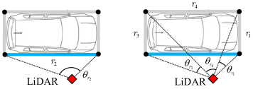
Figure 2: Illustration of the edge visibility and angles $\theta_{r_{n}}$. The blue color of region $r_{2}$ denotes that it is visible from the LiDAR, i.e., $b_{r_{2}}=1$.

III Particle-based Implementation of the Proposed Method

For the system model in Section II, a closed-form filtering recursion of the posterior PMBM density is difficult to obtain. Moreover, the standard linearization methods such as Taylor expansion and UT may not yield a feasible estimator due to the highly nonlinear eigen-decomposition required in the measurement model. Therefore, a particle-based implementation of the proposed PMRA-PMBM algorithm is considered in this section. The distribution of kinematic state $\mathbf{m}_{k}$ and extent state $E_{k}$ of a target is represented by a weighted set of particles $\Xi_{k}=\{(\mathbf{m}_{k}^{(l)},E_{k}^{(l)},w_{k}^{(l)})\}_{l=1}^{L}$, where $\sum_{l}w_{k}^{(l)}=1$. Note that a closed-form recursion based on gamma conjugate prior is used to estimate the measurement rate and $\gamma_{k}$ is not contained in the particles. Consequently, the distribution of state $\mathbf{x}_{k}$ can be represented by the PDF $\mathcal{F}(\mathbf{x}_{k};\alpha_{k},\beta_{k},\Xi_{k})$.

III-A Data Association Problem

Since the actual origins of measurements are unknown, the data association problem must be handled in the PMRA-PMBM algorithm. At time $k$, let the global hypotheses indexed by set $\mathbf{J}_{k}$ and denote the index set of existing targets in the $j$-th global hypothesis by $\mathbf{I}^{j}_{k}$. The measurement index set satisfies $\mathbf{M}_{k}\cap\mathbf{I}^{j}_{k}=\emptyset$ for all $j\in\mathbf{J}_{k}$. Let $\mathbb{A}^{j}_{k}$ be the space of all data associations in the $j$-th global hypothesis. Then, a data association $\mathbf{A}\in\mathbb{A}^{j}_{k}$ can be defined as partitioning the union set $\mathbf{M}_{k}\cup\mathbf{I}^{j}_{k}$ into disjoint nonempty subsets $\{\mathbf{S}\}$ that satisfy $\uplus_{\mathbf{S}\in\mathbf{A}}\mathbf{S}=\mathbf{M}_{k}\cup\mathbf{I}^{j}_{k}$ [11]. A subset $\mathbf{S}$ is called an index cell, which can contain any measurement indices $m\in\mathbf{M}_{k}$ and at most one target index $i_{\mathbf{S}}\in\mathbf{I}^{j}_{k}$, because a measurement cannot originate from more than one target in our system assumption. The measurements in index cell $\mathbf{S}$ are denoted by $\mathbf{Y}_{\mathbf{S}}=\{\mathbf{z}^{m}_{k}\}_{m\in\mathbf{S}\cap\mathbf{M}_{k}}$. Thus, if $i_{\mathbf{S}}\in\mathbf{S}$ and $\mathbf{Y}_{\mathbf{S}}\neq\emptyset$, $\mathbf{S}$ assigns the measurements $\mathbf{Y}_{\mathbf{S}}$ to the target $i_{\mathbf{S}}$; if $\mathbf{S}$ contains no target index, it assigns $\mathbf{Y}_{\mathbf{S}}$ to a newborn target or clutter; if $\mathbf{S}=\{i_{\mathbf{S}}\}$, it means that target $i_{\mathbf{S}}$ is not detected.

The computational complexity of the data association problem can be significantly reduced by eliminating improbable association hypotheses with clustering and gating. In the PMRA-PMBM filter, the measurements $\mathbf{Z}_{k}$ are first partitioned into disjoint clusters by the DBSCAN algorithm [24]. Next, a gating step is performed to identify the associations between clusters and targets. If a cluster $\mathbf{Y}\subseteq\mathbf{Z}_{k}$ contains measurements within a certain distance $d_{\mathrm{in}}$ around the predicted position of the $i$-th existing target, an index cell $\mathbf{S}$ can be formed by assigning $\mathbf{Y}_{\mathbf{S}}=\mathbf{Y}$ and $i_{\mathbf{S}}=i$. If the minimum distance from the center of a cluster $\mathbf{Y}^{b}\subseteq\mathbf{Z}_{k}$ to the predicted position of any existing target exceeds a certain threshold $d_{\mathrm{out}}$, the cluster is possibly originating from a newborn target. According to the clustering and gating results denoted by $\mathcal{CG}_{k}$, only a subset of all possible data associations is calculated at each time step. For further discussions on data association, clustering, and gating see, e.g., [9, 11, 4].

III-B Target State Initialization

The state of a newborn target is initialized when a new Poisson component is added to the PMBM density to represent a birth event. Each Poisson component models the state of an undetected target, and the PPP intensity $D^{u}(\mathbf{x})$ is maintained as the weighted sum of Poisson components. Specifically, $D^{u}(\mathbf{x})=\sum_{{h\in\mathbf{H}^{u}}}w^{u,h}\mathcal{F}(\mathbf{x};\alpha^{u,h},\beta^{u,h},\Xi^{u,h})$, where $w^{u,h}>0$ is the component weight, and $\mathbf{H}^{u}$ is an index set.

At time $k$, assume a set of measurements $\mathbf{Y}_{k}^{b}$ is used to initialize the state of a newborn target $\{\alpha^{b}_{k},\beta^{b}_{k},\Xi^{b}_{k}\}$. Then, the gamma parameters of the measurement rate $\gamma_{k}$ are assigned with predefined values $\alpha^{b}_{k}=\alpha^{b}$, $\beta^{b}_{k}=\beta^{b}$, and the kinematic part of particles $\Xi^{b}_{k}$ is obtained by sampling from the following proposal distributions

$$\mathbf{m}_{k}^{b,(l)}=\left[x_{k}^{b,(l)},y_{k}^{b,(l)},\dot{x}_{k}^{b,(l)},\dot{y}_{k}^{b,(l)},\omega_{k}^{b,(l)}\right]^{\mathrm{T}}$$ (23a)

$$[x_{k}^{b,(l)},y_{k}^{b,(l)}]^{\mathrm{T}}\sim\mathcal{N}(\bar{\mathbf{z}}_{k},Q_{\mathrm{pos}})$$ (23b)

$$[\dot{x}_{k}^{b,(l)},\dot{y}_{k}^{b,(l)}]^{\mathrm{T}}\sim\mathcal{N}(\dot{\mathbf{m}}_{k},Q_{\mathrm{vel}})$$ (23c)

$$\omega_{k}^{b,(l)}\sim\mathcal{N}(0,Q_{\mathrm{turn}})$$ (23d)

where $\bar{\mathbf{z}}_{k}=\sum_{\mathbf{z}\in\mathbf{Y}_{k}^{b}}\mathbf{z}/|\mathbf{Y}_{k}^{b}|$ is the approximated target position, $\dot{\mathbf{m}}_{k}$ is the approximated target velocity, $Q_{\mathrm{pos}}$, $Q_{\mathrm{vel}}$, and $Q_{\mathrm{turn}}$ are predefined covariance matrices.

The extent part of $\Xi^{b}_{k}$ is sampled from an inverse Wishart distribution with DOF parameter $q^{b}$ and scale matrix $V^{b}_{k}$:

$$E_{k}^{b,(l)}\sim\mathcal{IW}(q^{b},V^{b}_{k})$$ (24a)

$$V^{b}_{k}=(q^{b}-3)\mathrm{Rot}(\dot{\mathbf{m}}_{k})\begin{bmatrix}\bar{e}_{1}&0\\ 0&\bar{e}_{2}\end{bmatrix}\mathrm{Rot}(\dot{\mathbf{m}}_{k})^{\mathrm{T}}$$ (24b)

in which $\mathrm{Rot}(\dot{\mathbf{m}}_{k})$ denotes the 2D rotation matrix of the angle between $\dot{\mathbf{m}}_{k}$ and the axis $O_{\mathrm{G}}X_{\mathrm{G}}$; $\bar{e}_{1}$ and $\bar{e}_{2}$ are the expected length and width of the vehicle. Here, we assume that the orientation of the vehicle aligns with the direction of its velocity. Therefore, $\dot{\mathbf{m}}_{k}$ can be set based on an initial velocity close to the actual target motion for a robust initialization.

Finally, the particle weights are calculated by

$$w_{k}^{(l)}=\frac{\mathcal{N}([x_{k}^{(l)},y_{k}^{(l)}]^{\mathrm{T}};\bar{\mathbf{z}}_{k},Q_{\mathrm{pos}})}{\sum_{l}\mathcal{N}([x_{k}^{(l)},y_{k}^{(l)}]^{\mathrm{T}};\bar{\mathbf{z}}_{k},Q_{\mathrm{pos}})}.$$ (25)

III-C PMRA-PMBM Prediction

In the particle-based implementation of PMRA-PMBM, the state transition PDF defined in (11) is represented by $\mathcal{F}(\mathbf{x}_{+};\alpha_{+},\beta_{+},\Xi_{+})$ where the subscript $+$ is the abbreviation of $k|k-1$. The predicted gamma parameters $\alpha_{+}$, $\beta_{+}$ are given in (10), and the predicted particles and weights are

$$\mathbf{m}_{+}^{(l)}\sim\mathcal{N}(F_{k-1}\mathbf{m}_{k-1}^{(l)},G_{k-1}Q_{k-1}G_{k-1}^{\mathrm{T}})$$ (26a)

$$E_{+}^{(l)}\sim\mathcal{W}(q_{k-1},\frac{V(\omega_{k-1}^{(l)})E_{k-1}^{(l)}V(\omega_{k-1}^{(l)})^{\mathrm{T}}}{q_{k-1}})$$ (26b)

$$w_{+}^{(l)}=w_{k-1}^{(l)}.$$ (26c)

Given the posterior multi-target PMBM density at time $k-1$, the predicted multi-target density is also a PMBM density with parameters [11, Section IV.B]

$$D_{+}^{u},\{(C_{+}^{j},\{(r_{+}^{j,i},f_{+}^{j,i})\}_{i\in\mathbf{I}_{k-1}^{j}})\}_{j\in\mathbf{J}_{k-1}}.$$ (27)

Based on the assumptions in Table I, the pseudo code of PMRA-PMBM prediction is provided in Table II, where the time index $k-1$ is omitted for notational simplicity. The predicted PMBM density is obtained by applying the state transition model (10) and (26) to PPP and MBM densities. Different from the standard PMBM implementations (e.g.,[11]), the predicted PPP intensity $D_{+}^{u}$ of PMRA-PMBM does not include a predefined birth intensity $D^{b}_{+}$ with known parameters. Instead, the intensity of newborn target is calculated in the update procedure with clustering and gating results.

TABLE I: Assumptions of PMRA-PMBM

1. Empty initial PPP: $\mathbf{H}^{u}_{0}=\emptyset$.

2. Empty initial MBM: $\mathbf{J}_{0}=\{j_{1}\}$, $C_{0}^{j_{1}}=0$, and $\mathbf{I}^{j_{1}}_{0}=\emptyset$.

3. Probabilities of detection and survival can be approximated as $p_{\mathrm{D}}(\mathbf{x})\approx p_{\mathrm{D}}(\hat{\mathbf{x}})$ and $p_{\mathrm{S}}(\mathbf{x})\approx p_{\mathrm{S}}(\hat{\mathbf{x}})$, where $\hat{\mathbf{x}}=\int\mathbf{x}f(\mathbf{x})\mathrm{d}\mathbf{x}$.

4. Clutter Poisson rate $\mu^{c}$ is known and the spatial distribution is $f^{c}(\mathbf{z})=1/\mathrm{V}$, where $\mathrm{V}$ is the volume of the surveillance region.

TABLE II: PMRA-PMBM Prediction

Input: $D^{u},\{(C^{j},\{(r^{j,i},f^{j,i})\}_{i\in\mathbf{I}^{j}})\}_{j\in\mathbf{J}}$.

Output: $D_{+}^{u},\{(C_{+}^{j},\{(r_{+}^{j,i},f_{+}^{j,i})\}_{i\in\mathbf{I}^{j}})\}_{j\in\mathbf{J}}$.

Initialize: $D_{+}^{u}\leftarrow 0$

for $h\in\mathbf{H}^{u}$ do:

From $\alpha^{u,h}$, $\beta^{u,h}$, $\Xi^{u,h}$, compute $\alpha_{+}^{u,h}$, $\beta_{+}^{u,h}$, $\Xi_{+}^{u,h}$ by (10), (26).

Increment: $D^{u}_{+}\leftarrow D^{u}_{+}+w^{u,m}\mathcal{F}(\alpha_{+}^{u,h},\beta_{+}^{u,h},\Xi_{+}^{u,h})$

end for

for $j\in\mathbf{J}$ do:

for $i\in\mathbf{I}^{j}$ do:

From $\alpha^{j,i}$, $\beta^{j,i}$, $\Xi^{j,i}$, compute $\alpha_{+}^{j,i}$, $\beta_{+}^{j,i}$, $\Xi_{+}^{j,i}$ by (10), (26).

$f_{+}^{j,i}\leftarrow\mathcal{F}(\alpha_{+}^{j,i},\beta_{+}^{j,i},\Xi_{+}^{j,i})$, $r_{+}^{j,i}\leftarrow p_{\mathrm{S}}(\hat{\mathbf{x}}^{j,i})r^{j,i}$.

end for

$C_{+}^{j}\leftarrow C^{j}$

end for

III-D PMRA-PMBM Update

In the PMRA-PMBM update procedure, given the predicted density of a target $\mathcal{F}(\mathbf{x}_{+};\alpha_{+},\beta_{+},\Xi_{+})$ and a set of measurements $\mathbf{Y}$ associating with the target, the updated density $\mathcal{F}(\mathbf{x};\alpha,\beta,\Xi)$ is obtained as follows (the time index $k$ is omitted). First, the gamma parameters of measurement rate are updated with the Bayesian recursion in [18]:

$$\alpha=\alpha_{+}+|\mathbf{Y}|,\quad\beta=\beta_{+}+1,\quad\mathcal{L}_{\gamma}=\frac{\Gamma(\alpha)\beta_{+}^{\alpha_{+}}}{\Gamma(\alpha_{+})(\beta)^{\alpha}|\mathbf{Y}|!}$$ (28)

where $\Gamma(\cdot)$ is the gamma function, $\mathcal{L}_{\gamma}$ is the predictive likelihood. Then, the updated particles $\Xi$ are obtained from a simplified PMRA model, which processes the measurements in $\mathbf{Y}$ one by one instead of in a batch. In this way, the total number of measurement-region associations is reduced from $a=5^{|\mathbf{Y}|}$ to $a=5{|\mathbf{Y}|}$. Assign an arbitrary index order to the measurement set, i.e., $\mathbf{Y}=\{\mathbf{z}^{m}\}_{m=1}^{|\mathbf{Y}|}$. Then, for the measurement $\mathbf{z}^{m}$, the particle weights are updated by

$$w^{(l)}\propto w_{-}^{(l)}\sum_{n=1}^{5}\mathcal{L}_{r_{n}}(\mathbf{z}|\mathbf{m}_{-}^{(l)},E_{-}^{(l)})P\{r_{n}|\mathbf{m}_{-}^{(l)},E_{-}^{(l)}\}$$ (29)

where $\Xi_{-}=\{\mathbf{m}_{-}^{(l)},E_{-}^{(l)},w_{-}^{(l)}\}_{l=1}^{L}$ represents the particles and weights calculated with $\mathbf{z}^{m-1}$, and $\Xi_{-}=\Xi_{+}$ for $m=1$. The weights are normalized such that $\sum_{l}w^{(l)}=1$. Here, the conditional measurement likelihoods $\mathcal{L}_{r_{n}}$ are defined by (15) and (16); the prior association probability $P\{r_{n}|\mathbf{m}_{-}^{(l)},E_{-}^{(l)}\}$ is calculated with (22). If the effective particle number $1/\sum_{l}(w^{(l)})^{2}$ is below a threshold $L_{\mathrm{e}}$, systematic resampling is performed to resample the particles and avoid the particle degeneracy [25]. After all the measurements are processed, the predictive likelihood of particles is approximated by

$$\mathcal{L}_{\Xi}\approx\sum_{l=1}^{L}w_{-}^{(l)}\sum_{n=1}^{5}\mathcal{L}_{r_{n}}(\mathbf{z}|\mathbf{m}_{-}^{(l)},E_{-}^{(l)})P\{r_{n}|\mathbf{m}_{-}^{(l)},E_{-}^{(l)}\}.$$ (30)

At time $k$, given the predicted multi-target PMBM density parameterized by (27). According to the conjugacy property, the updated multi-target posterior is also a PMBM density. The update procedure of PMRA-PMBM includes four stages, and the corresponding pseudo code is shown in Table III.

In stage one, the algorithm performs clustering and gating with the predicted PMBM density and the measurement set. The clusters $\{\mathbf{Y}^{b,h}\}_{h\in\mathbf{H}^{b}}$ considered as possibly originating from the newborn targets are determined with the method in Section III-A. Note that the gating threshold $d_{\mathrm{out}}$ should be decreased if the target birth frequently occurs close to existing targets, and $d_{\mathrm{in}}$ should be increased for maneuvering targets.

In stage two, the algorithm calculates the density for undetected targets by updating the predicted PPP intensity $D_{+}^{u}$. Since the target is not associated with any measurement, the particles are directly propagated, and the mixture reduction method in [18] is used to calculate the gamma parameters.

In stage three, the algorithm generates data association hypotheses based on the clustering and gating results, then update the MBM density of the detected targets. Under the $j_{+}$-th global hypothesis, a cluster $\mathbf{Y_{S}}$ not associating with any existing targets (i.e, $\mathbf{S}\cap\mathbf{I}^{j_{+}}=\emptyset$) is used to calculate the density of a target detected for the first time. The updated density is multi-modal with one mode for each of the Poisson components in $D_{+}^{u}$. Therefore, gamma mixture reduction and

TABLE III: PMRA-PMBM Update

Input: $D_{+}^{u},\{(C_{+}^{j},\{(r_{+}^{j,i},f_{+}^{j,i})\}_{i\in\mathbf{I}_{+}^{j}})\}_{j\in\mathbf{J}_{+}}$, measurement set $\mathbf{Z}$.

Output: $D^{u},\{(C^{j},\{(r^{j,i},f^{j,i})\}_{i\in\mathbf{I}^{j}})\}_{j\in\mathbf{J}}$.

From $D_{+}^{u},\{(C_{+}^{j},\{(r_{+}^{j,i},f_{+}^{j,i})\}_{i\in\mathbf{I}^{j}})\}_{j\in\mathbf{J}}$ and $\mathbf{Z}$, compute clustering and gating results $\mathcal{CG}$.

Initialize: $D^{u}\leftarrow 0$, $D^{b}\leftarrow 0$, $\mathbf{J}\leftarrow\emptyset$, $j\leftarrow 0$, $h\leftarrow 0$.

for $h\in\mathbf{H}_{+}^{u}$ do: [PPP update for miss detected targets]

$q_{1}=1-p_{\mathrm{D}}(\hat{\mathbf{x}}_{+}^{u,h})$, $q_{2}=p_{\mathrm{D}}(\hat{\mathbf{x}}_{+}^{u,h})[\beta_{+}^{u,h}(\beta_{+}^{u,h}+1)]^{\alpha_{+}^{u,h}}$,

$q_{\mathrm{D}}=q_{1}+q_{2}$, $\beta^{u,h}=1/\{q_{1}/(q_{\mathrm{D}}\beta_{+}^{u,h})+q_{2}/[q_{\mathrm{D}}(\beta_{+}^{u,h}+1)]\}$,

$w^{u,h}=q_{\mathrm{D}}w_{+}^{u,h}$. $D^{u}\leftarrow D^{u}+w^{u,h}\mathcal{F}(\alpha_{+}^{u,h},\beta^{u,h},\Xi_{+}^{u,h})$.

end for

for $j_{+}\in\mathbf{J}_{+}$ do:

Compute associations $\mathbb{A}^{j_{+}}$ based on $\mathcal{CG}$.

for $\mathbf{A}\in\mathbb{A}^{j_{+}}$ do:

Increment: $j\leftarrow j+1$, $\mathbf{J}\leftarrow\mathbf{J}\cup j$.

Initialize: $\mathbf{I}^{j}\leftarrow\emptyset$, $i\leftarrow 0$, $\mathbf{D}\leftarrow\emptyset$, $\mathcal{L}_{\mathbf{A}}^{j_{+}}\leftarrow 1$.

for $\mathbf{S}\in\mathbf{A}$ do:

Increment: $i\leftarrow i+1$, $\mathbf{I}^{j}\leftarrow\mathbf{I}^{j}\cup i$.

if $\mathbf{S}\cap\mathbf{I}^{j_{+}}=\emptyset$ then: [PPP update for new detected targets]

for $h\in\mathbf{H}^{u}_{+}$ do:

From $\alpha^{u,h}_{+},\beta^{u,h}_{+},\Xi^{u,h}_{+}$ and $\mathbf{S}$, compute $\alpha^{u,h}$, $\beta^{u,h}$, $\Xi^{u,h}$,

$\mathcal{L}_{\gamma}^{u,h}$, $\mathcal{L}_{\Xi}^{u,h}$ as in (28), (29), (30).

end for

From $\{\alpha^{u,h},\beta^{u,h}\}_{h\in\mathbf{H}^{u}_{+}}$, compute $\alpha$, $\beta$ with gamma mix-

ture reduction.

From $\{\Xi^{u,h}\}_{h\in\mathbf{H}^{u}_{+}}$, compute $\Xi$ with systematic resampling.

$r=1$, $f=\mathcal{F}(\alpha,\beta,\Xi)$,

$\mathcal{L}=\sum_{h\in\mathbf{H}^{u}_{+}}w^{u,h}p_{\mathrm{D}}(\hat{\mathbf{x}}^{u,h})\mathcal{L}_{\gamma}^{u,h}\mathcal{L}_{\Xi}^{u,h}$.

else: [Bernoulli update for detected targets]

From $\alpha^{j_{+},i_{\mathbf{S}}}_{+},\beta^{j_{+},i_{\mathbf{S}}}_{+},\Xi^{j_{+},i_{\mathbf{S}}}_{+}$ and $\mathbf{S}$, compute $\alpha^{j_{+},i_{\mathbf{S}}}$,

$\beta^{j_{+},i_{\mathbf{S}}}$, $\Xi^{j_{+},i_{\mathbf{S}}}$, $\mathcal{L}_{\gamma}^{j_{+},i_{\mathbf{S}}}$, $\mathcal{L}_{\Xi}^{j_{+},i_{\mathbf{S}}}$ as in (28), (29), (30).

$r=1$, $f=\mathcal{F}(\alpha^{j_{+},i_{\mathbf{S}}},\beta^{j_{+},i_{\mathbf{S}}},\Xi^{j_{+},i_{\mathbf{S}}})$,

$\mathcal{L}=r^{j_{+},i_{\mathbf{S}}}_{+}p_{\mathrm{D}}(\hat{\mathbf{x}}^{j_{+},i_{\mathbf{S}}})\mathcal{L}_{\gamma}^{j_{+},i_{\mathbf{S}}}\mathcal{L}_{\Xi}^{j_{+},i_{\mathbf{S}}}$. $\mathbf{D}\leftarrow\mathbf{D}\cup i_{\mathbf{S}}$.

end if

$r^{j,i}\leftarrow r$, $f^{j,i}\leftarrow f$, $\mathcal{L}_{\mathbf{A}}^{j_{+}}\leftarrow\mathcal{L}_{\mathbf{A}}^{j_{+}}\times\mathcal{L}$.

end for

for $i_{+}\in(\mathbf{I}^{j_{+}}\backslash\mathbf{D})$ do: [Bernoulli update for miss-detected targets]

Increment: $i\leftarrow i+1$, $\mathbf{I}^{j}\leftarrow\mathbf{I}^{j}\cup i$.

$q_{2}=p_{\mathrm{D}}(\hat{\mathbf{x}}_{+}^{j_{+},i_{+}})[\beta_{+}^{j_{+},i_{+}}/(\beta_{+}^{j_{+},i_{+}}+1)]^{\alpha_{+}^{j_{+},i_{+}}}$,

$q_{1}=1-p_{\mathrm{D}}(\hat{\mathbf{x}}_{+}^{j_{+},i_{+}})$, $q_{\mathrm{D}}=q_{1}+q_{2}$.

$\beta=1/\{q_{1}/(q_{\mathrm{D}}\beta_{+}^{j_{+},i_{+}})+q_{2}/[q_{\mathrm{D}}(\beta_{+}^{j_{+},i_{+}}+1)]\}$.

$\mathcal{L}=1+r^{j_{+},i_{+}}(q_{\mathrm{D}}-1)$, $r=r^{j_{+},i_{+}}q_{\mathrm{D}}/\mathcal{L}$.

$r^{j,i}\leftarrow r$, $f^{j,i}\leftarrow\mathcal{F}(\alpha_{+}^{j_{+},i_{+}},\beta,\Xi_{+}^{j_{+},i_{+}})$, $\mathcal{L}_{\mathbf{A}}^{j_{+}}\leftarrow\mathcal{L}_{\mathbf{A}}^{j_{+}}\times\mathcal{L}$.

end for

$C^{j}\leftarrow\mathcal{L}_{\mathbf{A}}^{j_{+}}$.

end for

end for

$C^{j}\leftarrow C^{j}/\sum_{j^{\prime}\in\mathbf{J}}C^{j^{\prime}}$.

From $\mathcal{CG}$, compute clusters $\{\mathbf{Y}^{b,h}\}_{h\in\mathbf{H}^{b}}$.

for $h\in\mathbf{H}^{b}$ do: [PPP initialization for new birth targets]

Initialize: From $\mathbf{Y}^{b,h}$, compute $\Xi^{b,h}$ by (23), (24), and (25).

Increment: $D^{b}\leftarrow D^{b}+w^{b}\mathcal{F}(\mathbf{x};\alpha^{b},\beta^{b},\Xi^{b,h})$.

end for

$D^{u}\leftarrow D^{u}+D^{b}$, where $\mathbf{H}^{u}\leftarrow\mathbf{H}_{+}^{u}\cup\mathbf{H}^{b}$.

systematic resampling are applied to calculate a single set of Bernoulli parameters. If the cluster is associated with a detected target (i.e., $\mathbf{S}\cap\mathbf{I}^{j_{+}}=i_{\mathbf{S}}$), the predicted Bernoulli density of the target is updated by (28), (29), and (30), and the target index is stored in a detection set $\mathbf{D}$. The state update for a previously detected but now miss-detected target is similar to that of undetected targets in stage two. Note that $\mathbf{I}^{j_{+}}\backslash\mathbf{D}$ denotes excluding the detection set from the target index set.

In the final stage, the algorithm initializes the birth PPP intensity $D^{b}$ with the clusters $\{\mathbf{Y}^{b,h}\}_{h\in\mathbf{H}^{b}}$ and combines it into the updated PPP density $D^{u}$.

III-E Pruning and State Extraction

The multi-target state estimation is extracted from the PMBM density by a simple but effective method as proposed in [11, 4]. After the PMBM update at time $k$, the $j_{\max}$-th MB density with the largest weight $C^{j_{\max}}_{k|k}$ is selected to represent the best global hypothesis. For a Bernoulli component $f^{j_{\max},i}_{k|k}$ in this MB density, if the existing probability $r^{j_{\mathrm{max}},i}_{k|k}$ exceeds a threshold $r_{\mathrm{th}}$, then the kinematic and extent state of the $i$-th target is estimated by

$$\hat{\mathbf{m}}_{k|k}=\sum_{l=1}^{L}w_{k|k}^{(l)}\mathbf{m}_{k|k}^{(l)},\quad\hat{E}_{k|k}=\sum_{l=1}^{L}w_{k|k}^{(l)}E_{k|k}^{(l)}.$$ (31)

The PMRA-PMBM filtering recursion will continuously add new Poisson and MB components in the PMBM density. Therefore, after performing state extraction, the Poisson and MB components with low weights are removed. With appropriate pruning thresholds, this procedure can reduce the computational complexity without sacrificing the tracking performance [11].

IV Simulation Study

In this section, the tracking performance of PMRA-PMBM algorithm is evaluated with simulated data. As illustrated in Fig. 3, we simulate a typical application scenario of the intelligent transportation system, where a LiDAR sensor is mounted on the road side unit to monitor the traffic at the intersection [26][27]. During the $20\mathrm{s}$ simulation period, $6$ vehicles with $4.5\mathrm{m}\times 1.8\mathrm{m}$ rectangular extent enter and leave the surveillance area at different time steps. A stationary LiDAR sensor with $2\mathrm{Hz}$ sample rate and $0.5^{\circ}$ angular resolution collects measurement points of the vehicles. We assume that the target-originated measurements are reflected from the visible edges of extent rectangles, and the covariance of additive zero-mean Gaussian measurement noise is $\mathrm{diag}([(0.1^{\circ})^{2},(0.01\mathrm{m})^{2}])$. The clutters are uniformly distributed over the $100\mathrm{m}\times 100\mathrm{m}$ surveillance area with Poisson rate $\mu^{c}=20$.

Figure 3: Visualization of the simulation scenario. The target extent at the start or end of a trajectory (solid line) is represented by a black rectangle, with the corresponding time indicated next to it.

The generalized optimal sub-pattern assignment (GOSPA) metric [28], which can measure the localization errors of detected targets and the cardinality errors due to missed and false targets, is applied to evaluate the tracking performance. Specifically, we use the GOSPA based on Euclidean distance $d_{\mathrm{E}}$ and Hausdorff distance $d_{\mathrm{H}}$ to calculate the estimation errors of the target’s center position and extent. Given the estimated center position and extent vertices for a target as $\hat{\mathbf{p}}^{0}$ and $\hat{\mathcal{P}}=\{\hat{\mathbf{p}}^{n}\}_{n=1}^{4}$, the distances are defined by

$$d_{\mathrm{E}}(\hat{\mathbf{p}}^{0},\mathbf{p}^{0})=\sqrt{(\hat{x}^{0}-x^{0})^{2}+(\hat{y}^{0}-y^{0})^{2}}$$ (32)

$$d_{\mathrm{H}}(\hat{\mathcal{P}},\mathcal{P})=\max\left\{\underset{\hat{\mathbf{p}}\in\hat{\mathcal{P}}\ \mathbf{p}\in\mathcal{P}}{\max\min}d_{\mathrm{E}}(\hat{\mathbf{p}},\mathbf{p}),\underset{\mathbf{p}\in\mathcal{P}\ \hat{\mathbf{p}}\in\hat{\mathcal{P}}}{\max\min}d_{\mathrm{E}}(\hat{\mathbf{p}},\mathbf{p})\right\}$$

where $\mathbf{p}^{0}$ and $\mathcal{P}$ are the ground truth. The other GOSPA parameters are $c=5$, $p=1$, and $\alpha=2$.

The proposed PMRA-PMBM filter is compared with the DRA-PMBM (an implementation of “Model-V” DRA method [14] under the PMBM framework) and the GGIW-PMBM [11] filters in the simulation scenario. All three algorithms use the CT model to track target kinematic state, and the prior target extent is set as $4\mathrm{m}\times 2\mathrm{m}$. The particle number and resample threshold of the PMRA-PMBM filter are $L=1000$ and $L_{\mathrm{e}}=100$. The other parameters are fine-tuned for each algorithm to obtain the optimal performance.

The GOSPA results averaged over 100 Monte Carlo runs are shown in Fig. 4 and Table IV. The PMRA-PMBM has overall lower estimation error for target position and extent than the other algorithms, especially the GGIW-PMBM which assumes measurements are Gaussian distributed over the target extent. Compared to the DRA-PMBM, the GOSPA of PMRA-PMBM decreases faster after $2$ targets appear at $5\mathrm{s}$ and exhibits less fluctuation when target cardinality changes frequently between $9\mathrm{s}$ and $15\mathrm{s}$. This indicates that the PMRA-PMBM has superior estimation accuracy and stability in a rapidly changing MTT scenario. As illustrated by Fig. 5, the PMRA-PMBM filter can accurately estimates the vehicle extent from the simulated LiDAR point cloud. However, the particle-based implementation of the PMRA-PMBM requires more compuational resources than the other two algorithms. As shown in Table IV, the average processed frames per second (FPS) of PMRA-PMBM is about 47.5% that of DRA-PMBM and 15.1% that of GGIW-PMBM on the same simulation platform.

(a) GOSPA based on Euclidean Distance

(b) GOSPA based on Hausdorff Distance

Figure 4: GOSPA for PMRA-PMBM, DRA-PMBM and GGIW-PMBM in the scenario of Fig. 3, averaged over 100 Monte Carlo simulations.

Figure 5: Extent estimates of the same target in a Monte Carlo simulation. Grey rectangles are the true extents, and cyan circles are the LiDAR measurements. The estimation results of PMRA-PMBM, DRA-PMBM, and GGIW-PMBM are shown by red solid, blue dashed, and black dotted rectangles, respectively.

TABLE IV: FPS and Mean GOSPA of Different Algorithms

Algorithm	Mean GOSPA-E	Mean GOSPA-H	FPS
PMRA-PMBM	0.89	1.41	6.42
DRA-PMBM	1.81	2.70	13.51
GGIW-PMBM	3.29	5.35	42.55
The bold values indicate the best result in each column.

V Conclusion

This paper presents the PMRA-PMBM filter for tracking multiple vehicles with LiDAR point clouds. The proposed PMRA model improves the estimation accuracy and stability of extended target state compared with the existing DRA methods. Simulation results show that the particle-based implementation of the PMRA-PMBM filter can achieve superior estimation accuracy in both the position and extent of vehicle compared to the GGIW-PMBM and DRA-PMBM filters. In our future work, message passing methods and the parallelized particle filter will be investigated to reduce the computational complexity of the proposed algorithm.

References

- [1] W. Xiong, J. Liu, Y. Xia, T. Huang, B. Zhu, and W. Xiang, “Contrastive learning for automotive mmWave radar detection points based instance segmentation,” in Proc. IEEE Int. Conf. Intel. Trans. Sys. (ITSC), 2022, pp. 1255-1261.
- [2] J. Liu, Q. Zhao, W. Xiong, T. Huang, Q.-L. Han, and B. Zhu, “SMURF: Spatial multi-representation fusion for 3D object detection with 4D imaging radar,” IEEE Trans. Intell. Veh., vol. 9, no. 1, pp. 799-812, Jan. 2024.
- [3] W. Xiong, J. Liu, T. Huang, Q. Han, Y. Xia, and B. Zhu, “LXL: LiDAR excluded lean 3D object detection with 4D imaging radar and camera fusion,” IEEE Trans. Intell. Veh., vol. 9, no. 1, pp. 79-92, Jan. 2024.
- [4] J. Liu, L. Bai, Y. Xia, T. Huang, B. Zhu, and Q.-L. Han, “GNN-PMB: A simple but effective online 3D multi-object tracker without bells and whistles,” IEEE Trans. Intell. Veh., vol. 8, no. 2, pp. 1176-1189, Feb. 2023.
- [5] Z. Zhang, J. Liu, Y. Xia, T. Huang, Q.-L. Han, and H. Liu, “LEGO: Learning and graph-optimized modular tracker for online multi-object tracking with point clouds,” arXiv preprint, 2023. [Online]. Available: arxiv.org/abs/2308.09908.
- [6] F. Meyer and J. Williams, “Scalable detection and tracking of geometric extended objects,” IEEE Trans. Signal Process., vol. 69, pp. 6283–6298, Oct. 2021.
- [7] P. Dahal, S. Mentasti, S. Arrigoni, F. Braghin, M. Matteucci and F. Cheli, “Extended object tracking in curvilinear road coordinates for autonomous driving,” IEEE Trans. Intell. Veh., vol. 8, no. 2, pp. 1266-1278, Feb. 2023.
- [8] J. Liu, G. Ding, Y. Xia, J. Sun, T. Huang, L. Xie, and B. Zhu, “Which framework is suitable for online 3d multi-object tracking for autonomous driving with automotive 4d imaging radar?” arXiv preprint, 2023. [Online]. Available: arxiv.org/abs/2309.06036.
- [9] K. Granström and M. Baum, “A tutorial on multiple extended object tracking,” TechRxiv preprint, 2022. [Online]. Avaliable: www.techrxiv.org/doi/full/10.36227/techrxiv.19115858.v1.
- [10] S. Yang and M. Baum, “Tracking the orientation and axes lengths of an elliptical extended object,” IEEE Trans. Signal Process., vol. 67, no. 18, pp. 4720–4729, Sep. 2019.
- [11] K. Granstrom, M. Fatemi, and L. Svensson, “Poisson multi-Bernoulli mixture conjugate prior for multiple extended target filtering,” IEEE Trans. Aerosp. Electron. Syst., vol. 56, no. 1, pp. 208–225, Feb. 2020.
- [12] M. Baum and U. D. Hanebeck, “Extended object tracking with random hypersurface models,” IEEE Trans. Aerosp. Electron. Syst., vol. 50, no. 1, pp. 149-159, Jan. 2014.
- [13] H. Xu, Y. Li, Y. Ke, Z. Jiang and Y. Liu, “A novel method for maneuvering extended vehicle tracking with automotive radar,” in Proc. IEEE Int. Conf. Inf. Fusion (FUSION), 2023, pp. 1-7.
- [14] X. Cao, J. Lan, X. R. Li, and Y. Liu, “Automotive radar-based vehicle tracking using data-region association,” IEEE Trans. Intell. Transp. Syst., vol. 23, no. 7, Jul. 2022.
- [15] Y. Xia, Á. F. García-Fernández, F. Meyer, J. L. Williams, K. Granström and L. Svensson, “Trajectory PMB filters for extended object tracking using belief propagation,” IEEE Trans. Aerosp. Electron. Syst., vol. 59, no. 6, pp. 9312-9331, Dec. 2023.
- [16] Y. Xia, K. Granström, L. Svensson, M. Fatemi, Á. F. García-Fernández and J. L. Williams, “Poisson multi-Bernoulli approximations for multiple extended object filtering,” IEEE Trans. Aerosp. Electron. Syst., vol. 58, no. 2, pp. 890-906, Apr. 2022.
- [17] X. R. Li and V. P. Jilkov, “Survey of maneuvering target tracking. Part I: dynamic models,” IEEE Trans. Aerosp. Electron. Syst., vol. 39, no. 4, pp. 1333–1364, Oct. 2003.
- [18] K. Granström and U. Orguner, “Estimation and maintenance of measurement rates for multiple extended target tracking,” in Proc. IEEE Int. Conf. Inf. Fusion (FUSION), 2012, pp. 2170-2176.
- [19] B. Douillard et al., “On the segmentation of 3D LiDAR point clouds,” in Proc. IEEE Int. Conf. Robot. Autom. (ICRA), 2011, pp. 2798-2805.
- [20] D. Zermas, I. Izzat and N. Papanikolopoulos, “Fast segmentation of 3D point clouds: A paradigm on LiDAR data for autonomous vehicle applications,” in Proc. IEEE Int. Conf. Robot. Autom. (ICRA), 2017, pp. 5067-5073.
- [21] S. J. Julier and J. K. Uhlmann, “Unscented filtering and nonlinear estimation,” Proceedings of the IEEE, vol. 92, no. 3, Mar. 2004.
- [22] P. Berthold, M. Michaelis, T. Luettel, D. Meissner, and H.-J. Wuensche, “Probabilistic vehicle tracking with sparse radar detection measurements,” J. Adv. Inf. Fusion, vol 17, 2, 2022.
- [23] P. Berthold, M. Michaelis, T. Luettel, D. Meissner and H. -J. Wuensche, “A continuous probabilistic origin association filter for extended object tracking,” in Proc. IEEE Int. Conf. Multisens. Fusion Integr. Intell. Syst. (MFI), 2020, pp. 323-329.
- [24] E. Schubert, J. Sander, M. Ester, H. P. Kriegel, and X. Xu, “DBSCAN revisited, revisited: Why and how you should (still) use DBSCAN,” ACM Trans. Database Syst., vol. 42, no. 3, pp. 1–21, Sep. 2017.
- [25] J. Elfring, E. Torta, and R. Van De Molengraft, “Particle filters: A hands-on tutorial,” Sensors, vol. 21, no. 2, p. 438, Jan. 2021.
- [26] W. Jiang, et al., “Optimizing the placement of roadside LiDARs for autonomous driving,” in Proc. IEEE/CVF Int. Conf. Comput. Vis. (ICCV), 2023, pp. 18335-18344
- [27] T. Huang, J. Liu, X. Zhou, D. C. Nguyen, M. R. Azghadi, Y. Xia, Q.-L. Han, and S. Sun, “V2X cooperative perception for autonomous driving: Recent advances and challenges,” arXiv preprint, 2023. [Online]. Available: arxiv.org/abs/2310.03525.
- [28] A. S. Rahmathullah, Á. F. García-Fernández and L. Svensson, “Generalized optimal sub-pattern assignment metric,” in Proc. IEEE Int. Conf. Inf. Fusion (FUSION), 2017, pp. 1-8.