Causal Multi-Label Feature Selection in Federated Setting

Abstract

Multi-label feature selection serves as an effective mean for dealing with high-dimensional multi-label data. To achieve satisfactory performance, existing methods for multi-label feature selection often require the centralization of substantial data from multiple sources. However, in Federated setting, centralizing data from all sources and merging them into a single dataset is not feasible. To tackle this issue, in this paper, we study a challenging problem of causal multi-label feature selection in federated setting and propose a Federated Causal Multi-label Feature Selection (FedCMFS) algorithm with three novel subroutines. Specifically, FedCMFS first uses the FedCFL subroutine that considers the correlations among label-label, label-feature, and feature-feature to learn the relevant features (candidate parents and children) of each class label while preserving data privacy without centralizing data. Second, FedCMFS employs the FedCFR subroutine to selectively recover the missed true relevant features. Finally, FedCMFS utilizes the FedCFC subroutine to remove false relevant features. The extensive experiments on 8 datasets have shown that FedCMFS is effect for causal multi-label feature selection in federated setting.

1 Introduction

Multi-label learning has gradually become a research hotspot in the field of machine learning  [1, 2]. As information technology rapidly develops, data is becoming increasingly complex. Multi-label data is inevitably affected by redundancy and irrelevant features, potentially leading to the curse of dimensionality [3]. Therefore, feature selection, as one of the effective tools to solve the curse of dimensionality, is widely used in multi-label learning [4]. It aims to reduce the dimensionality of features by designing a metric for feature importance, with the goal of selecting a subset of features that contains irrelevant or redundant features as few as possible.

Existing multi-label feature selection algorithms are typically based on statistical co-occurrence relationships to determine feature dependency without providing an explanation for why they are dependent. To tackle this issue, researchers have proposed causal multi-label feature selection algorithms based on causal structures [5]. The causal relationship describes the causal relationship between two variables, revealing the underlying mechanisms of how these variables interact. A causal structure always employ a Directed Acyclic Graphs (DAG) to represent causal relationships between variables. In a DAG, the existence of a directed edge from A to B signifies that A is the parent (direct cause) of B, and conversely, B is the child (direct effect) of A [6]. Since local causal structure learning methods can directly find the parents and children of a given label variable and have better efficiency than global causal structure algorithms, which are often used in causal multi-label feature selection.

Currently those existing multi-label feature selection algorithms typically require access to all the data in order to determine important features and do not consider the data privacy. However, in many real-world application scenarios, data often originates from multiple sources, and the aggregation of data requires consideration of data privacy. For instance, chronic disease research may require patient data from various hospitals, leading to the risk of leaking patient data privacy.

To protect data privacy, federated learning has garnered considerable attention [7]. Federated learning builds machine learning models through multi-party collaboration and is primarily divided into vertical federated learning and horizontal federated learning. Vertical federated learning shares the same samples but each client holds different features, while clients in horizontal federated learning share the same feature space while holding different samples [8]. In this study, we consider the horizontal federated learning setting.

Since currently there are no studies on multi-label feature selection for considering data privacy, to fill this gap, in this paper, we propose the Federated Causal Multi-label Feature Selection (FedCMFS) algorithm in federated setting, which comprises three subroutines: the Federated Causal Feature Learning subroutine (FedCFL), the Federated Causal Feature Retrieval subroutine (FedCFR), and the Federated Causal Feature Correction subroutine (FedCFC). And we demonstrate the effectiveness of FedCMFS by simulating the federated setting with a large number of real datasets as well as conducting experiments using a variety of comparison algorithms.

2 Related work

In recent years, many scholars have proposed various multi-label feature selection algorithms to address the curse of dimensionality and improve prediction accuracy [9, 10]. Multi-label feature selection algorithms are generally classified into four major categories [11]: methods based on mutual information, methods based on regularization, methods based on manifold learning, and methods based on causal structure learning. Methods based on mutual information, such as FIMF [12], SCLS [13], and SRLG-LMA [14], select the most relevant features by measuring the mutual information relationship between features and labels. Methods based on regularization, such as SFUS [15], JFSC [16], and MLFS-GLOCAL [17], constrain the complexity of the model by introducing regularization terms, thereby selecting the most important features. Methods based on manifold learning, such as MCLS [18], MSSL [19], and MDFS [20], select features with important information by considering the local geometric structure and manifold characteristics of the data. Methods based on causal structure learning, such as MB-MCF [5], explore causal relationships between variables to construct a potential causal structure and select causally relevant features.

Recently, Fan et al. proposed a new method called LCIFS [21], which integrates manifold learning, adaptive spectral graph, and redundancy analysis into an ensemble framework to learn relevant information for multi-label feature selection. LCIFS utilizes the structural correlation of labels and simultaneously controls the use of redundant features, thereby achieving multi-label feature selection with a clear objective function.

In addition to algorithms targeting individual datasets, there is a series of work that can directly achieve multi-label feature selection from multiple datasets, but most of them do not consider data privacy issues.

In recent years, some scholars have focused on feature selection in federated learning. Federated learning can implement algorithms on multiple datasets while preserving privacy. Specifically, Hu et al. proposed a multi-participant federated evolutionary feature selection algorithm [22] for imbalanced data under privacy protection. They introduced a multi-level joint sample filling strategy to address imbalanced or empty classes on each participant. Subsequently, a federated evolutionary feature selection method based on supervised particle swarm optimization with multiple participants was proposed by periodically sharing the optimal feature subset among participants. Banerjee et al. introduced an information-theoretic multi-label feature selection method called Fed-FiS [23]. Fed-FiS evaluates feature-feature mutual information and feature-class mutual information to obtain local feature subsets and a global feature set.

In summary, some feature selection algorithms have been proposed in federated environments, but they have not considered feature selection in multi-label scenarios and have not addressed causal relationships between labels and labels, labels and features, and features and features. Therefore, this paper proposes a novel causal multi-label feature selection algorithm considering data privacy issues.

3 Notations and definitions

In this section, we initially present some key concepts and symbols related to Bayesian networks in the federated setting. We define $F=\{F_{1},F_{2},\ldots,F_{m}\}$ as a set of $m$ features, $Y=\{Y_{1},Y_{2},\ldots,Y_{q}\}$ as a set of $q$ labels, and $V=Y\cup F=\{V_{1},V_{2},\ldots,V_{m+q}\}$ as the node set encompassing all labels and features. Assuming that there are $N$ clients, with each client’s local data having a sample size of $W_{n},n=1,2,\ldots,N$. During the interaction process within the federated environment, the server sends a triplet $<Y_{i},V_{k},CS>$ to instruct each client to perform the conditional independence test between $Y_{i}$ and $V_{k}$ under the condition of $CS$ ($CS$ is the conditional set, which can be empty set $\emptyset$). Each client returns the correlation value $C_{n,<V_{i},V_{k},CS>}$ and the P value $P_{n,<V_{i},V_{k},CS>}$, enabling the server to aggregate the results into the corresponding weighted correlation value $C_{<V_{i},V_{k},CS>}$ and weighted P value $P_{<V_{i},V_{k},CS>}$. The significance level of the conditional independence test is denoted by $\alpha$ ($\alpha=0.05$). The notation $V_{i}\mathbin{\mathchoice{\hbox to0.0pt{\hbox{\set@color$\displaystyle\perp$}\hss}\kern 3.46875pt{}\kern 3.46875pt\hbox{\set@color$\displaystyle\perp$}}{\hbox to0.0pt{\hbox{\set@color$\textstyle\perp$}\hss}\kern 3.46875pt{}\kern 3.46875pt\hbox{\set@color$\textstyle\perp$}}{\hbox to0.0pt{\hbox{\set@color$\scriptstyle\perp$}\hss}\kern 2.36812pt{}\kern 2.36812pt\hbox{\set@color$\scriptstyle\perp$}}{\hbox to0.0pt{\hbox{\set@color$\scriptscriptstyle\perp$}\hss}\kern 1.63437pt{}\kern 1.63437pt\hbox{\set@color$\scriptscriptstyle\perp$}}}V_{j}\mid CS$ (where $i\neq j$ and $CS\subset V\setminus\{V_{i},V_{j}\}$) signifies that $V_{i}$ is conditionally independent from $V_{j}$ given $CS$, while $V_{i}\mathbin{\mathchoice{\hbox to0.0pt{\hbox{\set@color$\displaystyle\perp$}\hss}\kern 3.46875pt{\not}\kern 3.46875pt\hbox{\set@color$\displaystyle\perp$}}{\hbox to0.0pt{\hbox{\set@color$\textstyle\perp$}\hss}\kern 3.46875pt{\not}\kern 3.46875pt\hbox{\set@color$\textstyle\perp$}}{\hbox to0.0pt{\hbox{\set@color$\scriptstyle\perp$}\hss}\kern 2.36812pt{\not}\kern 2.36812pt\hbox{\set@color$\scriptstyle\perp$}}{\hbox to0.0pt{\hbox{\set@color$\scriptscriptstyle\perp$}\hss}\kern 1.63437pt{\not}\kern 1.63437pt\hbox{\set@color$\scriptscriptstyle\perp$}}}V_{j}\mid CS$ indicates that $V_{i}$ and $V_{j}$ are dependent given $CS$. The term $PC(Y_{i})$ represents the set of local causal structure (parent-child node set) for the label $Y_{i}$.

Table 1: Summary of Notation

Symbol	Meaning
$Y$	a set of labels
$F$	a set of features
$V$	$V=Y\cup F$
$q$	the number of labels
$m$	the number of features
$N$	the number of clients
$Y_{i}$	a label in $Y$
$F_{i}$	a feature in $F$
$V_{i}$	a node in $V$
$W_{n}$	the sample size of the local data for the $n$th client ($n=1,2,\ldots,N$)
$<Y_{i},V_{k},CS>$	the triplet sent by the server
$C_{n,<V_{i},V_{k},CS>}$	the correlation value between $Y_{i}$ and $V_{k}$ computed by the $n$th client under the $CS$ condition set
$C_{<V_{i},V_{k},CS>}$	the weighted correlation value
$P_{n,<V_{i},V_{k},CS>}$	the P value between $Y_{i}$ and $V_{k}$ computed by the $n$th client under the $CS$ condition set
$P_{<V_{i},V_{k},CS>}$	the weighted P value
$\alpha$	the significance level of the CI test
$V_{i}\mathbin{\mathchoice{\hbox to0.0pt{\hbox{\set@color$\displaystyle\perp$}\hss}\kern 2.36812pt{}\kern 2.36812pt\hbox{\set@color$\displaystyle\perp$}}{\hbox to0.0pt{\hbox{\set@color$\textstyle\perp$}\hss}\kern 2.36812pt{}\kern 2.36812pt\hbox{\set@color$\textstyle\perp$}}{\hbox to0.0pt{\hbox{\set@color$\scriptstyle\perp$}\hss}\kern 1.59769pt{}\kern 1.59769pt\hbox{\set@color$\scriptstyle\perp$}}{\hbox to0.0pt{\hbox{\set@color$\scriptscriptstyle\perp$}\hss}\kern 1.08406pt{}\kern 1.08406pt\hbox{\set@color$\scriptscriptstyle\perp$}}}V_{j}\mid CS$	$V_{i}$ and $V_{j}$ are independent under the $CS$ condition set
$V_{i}\mathbin{\mathchoice{\hbox to0.0pt{\hbox{\set@color$\displaystyle\perp$}\hss}\kern 2.36812pt{\not}\kern 2.36812pt\hbox{\set@color$\displaystyle\perp$}}{\hbox to0.0pt{\hbox{\set@color$\textstyle\perp$}\hss}\kern 2.36812pt{\not}\kern 2.36812pt\hbox{\set@color$\textstyle\perp$}}{\hbox to0.0pt{\hbox{\set@color$\scriptstyle\perp$}\hss}\kern 1.59769pt{\not}\kern 1.59769pt\hbox{\set@color$\scriptstyle\perp$}}{\hbox to0.0pt{\hbox{\set@color$\scriptscriptstyle\perp$}\hss}\kern 1.08406pt{\not}\kern 1.08406pt\hbox{\set@color$\scriptscriptstyle\perp$}}}V_{j}\mid CS$	$V_{i}$ and $V_{j}$ are dependent under the $CS$ condition set
$PC(Y_{i})$	the parent and children set of the label variable $Y_{i}$

Definition 3.1.

(Bayesian Network, BN) [24]. Let $P(V)$ be the joint probability distribution over $V$ and $G=(V,E)$ represent a directed acyclic graph (DAG) with nodes $V$ and edges $E$. The triplet $<V,G,P(V)>$ is called a BN if and only if $<V,G,P(V)>$ satisfies the Markov condition: every node of $G$ is independent of any subset of its non-descendants conditioning on the parents of the node.

In a DAG of BN, if there is a directed edge from A to B, A is the direct cause of B and B is the direct effect of A, then the DAG is called a causal DAG (i.e. causal structure)  [6].

Definition 3.2.

(Parent and Child, PC [6]). The parents and children of variable $V_{i}$ in a causal structure consists of the parents and children of $V_{i}$, called $PC(V_{i})$.

Definition 3.3.

(Markov blanket, MB [6]). The MB of a variable in a causal structure consists of the variable’s parents (direct causes), children (direct effects), and spouses (other parents of the variable’s children).

Theorem 3.1.

[6] In a DAG, given the MB of variable $V_{i}$,$MB(V_{i})$, for $\forall V_{j}\in V\setminus(MB(V_{i})\cup V_{i})$, $V_{i}$ is conditionally independent of $V_{j}$ given $MB(V_{i})$.

Theorem 3.1 indicates that in classification tasks, the MB of the label variable is the optimal feature subset for predicting the label variable [25]. Furthermore, recent studies suggest that in real-world scenarios, the prediction quality of the label variable’s PC set is almost identical to that of the MB of the class variable. Therefore, we employ the local causal structure learning algorithm, HITON-PC [26] to learn the PC set of the class variables.

Figure 1: The MB of node A consisting of B,C,D,E. The PC set of A comprising B, C, and D.

4 Proposed FedCMFS Algorithm

4.1 Overview of the FedCMFS Algorithm

In this paper, we simulate a federated environment using a client-server architecture, and propose the FedCMFS algorithm for causal multi-label feature selection in the federated setting. FedCMFS is a horizontal federated learning algorithm, which uses a central server and multiple clients to perform causal feature selection on standard multi-label data. Specifically, FedCMFS sequentially executes the following three subroutines to select causal features: (1) Federated Causal Feature Learning algorithm (FedCFL); (2) Federated Causal Feature Retrieval algorithm (FedCFR); (3) Federated Causal Feature Correction algorithm (FedCFC).

FedCFL treats both labels and features as ordinary variables, and it independently computes local causal variables for each label on each client. Throughout local causal structural learning, clients continuously interact with the server, ultimately obtaining causally relevant feature sets for all label variables: $PC\left(Y\right)=\{CPC\left(Y_{1}\right),CPC\left(Y_{2}\right),...,CPC\left(Y_{q}\right)\}$ for all labels on the server.

To tackle the issue of missing true relevant features, in FedCFR, the server communicate with each client to filter and detect potentially omitted features, obtaining an updated causally relevant feature sets for all label variables: $PC_{SR}=\{PC\left(Y_{1}\right),PC\left(Y_{2}\right),\ldots,PC\left(Y_{q}\right)\}$ with retrieved missing information on the server.

Considering the inconsistent data quality in each client, utilizing the principle of symmetry, FedCFC selectively corrects false causally relevant features in $PC_{SR}$ and achieves the final feature set $sel=PC\left(Y_{1}\right)\cup PC\left(Y_{2}\right)\cup\ldots\cup PC\left(Y_{q}\right)$.

4.2 Federated Causal Feature Learning algorithm (FedCFL)

HITON-PC is a widely used algorithm for learning a PC set of a given variable from a single-label dataset, which adopts a forward-backward strategy, exhibiting notable efficiency in causal feature learning. In this paper, we extend HITION-PC to the learn PC set of a label variable in federated setting and propose the federated causal feature learning algorithm, FedCFL, to address the causal multi-label feature selection problem in federated setting.

A simple strategy for applying the HITON-PC algorithm to multi-label feature selection in the federated setting is that each client learns a PC set independently for each label variable, and then aggregates the PC sets at the service. However, due to the different quality of samples from different clients, the PC sets learned by different client are often different. Therefore, to perform multi-label feature selection in the federated setting, we design the FedCFL algorithm consisting of two learning phases, as shown in Alg. 1.

Algorithm 1 FedCFL Algorithm

0: $Y$, $C=\{C_{1},C_{2},\ldots,C_{N}\}$

0: $PC(Y)$//Phase I: Identify potential PC variables of each label

1: for $\forall$ $C_{n}\in C$ do

2:    for $\forall Y_{i}\in Y$ do

3:       for $\forall V_{k}\in V\setminus Y_{i}$ do

4:          Calculate $C_{n,<Y_{i},V_{k},\emptyset>}$ and $P_{n,<Y_{i},V_{k},\emptyset>}$ and add them to $M_{n,i}^{\prime}$;

5:       end for

6:    end for

7:    Send $M_{n}^{\prime}$ to the server;

8: end for

9: $M\leftarrow$ The server merges, prunes, and sorts $M^{\prime}$ ;//Phase II: Execute forward-backward strategy to update CPC($Y_{i}$)

10: for $\forall M_{i}\in M$ do

11:    for $\forall V_{j}\in M_{i}$ do

12:       Add $V_{j}$ to $CPC(Y_{i})$;

13:       for $\forall V_{k}\in CPC(Y_{i})$ do

14:          if there exists $Z\subseteq CPC(Y_{i})$ such that $Y_{i}\mathbin{\mathchoice{\hbox to0.0pt{\hbox{\set@color$\displaystyle\perp$}\hss}\kern 2.36812pt{}\kern 2.36812pt\hbox{\set@color$\displaystyle\perp$}}{\hbox to0.0pt{\hbox{\set@color$\textstyle\perp$}\hss}\kern 2.36812pt{}\kern 2.36812pt\hbox{\set@color$\textstyle\perp$}}{\hbox to0.0pt{\hbox{\set@color$\scriptstyle\perp$}\hss}\kern 1.59769pt{}\kern 1.59769pt\hbox{\set@color$\scriptstyle\perp$}}{\hbox to0.0pt{\hbox{\set@color$\scriptscriptstyle\perp$}\hss}\kern 1.08406pt{}\kern 1.08406pt\hbox{\set@color$\scriptscriptstyle\perp$}}}V_{k}\mid Z$ then

15:             Remove $V_{k}$ from $CPC(Y_{i})$;

16:          end if

17:       end for

18:    end for

19: end for

20: $PC(Y)=\{CPC(Y_{1}),CPC(Y_{2}),...,CPC(Y_{q})\}$;

21: return  $PC(Y)$

In Phase I of FedCFL, we initially identify potential PC variables for each class label. The computation for this phase is carried out at each client and ultimately converges at the server. Assuming that there are $N$ clients (denoted as client 1, client 2, …, client N) and one server. At the beginning of phase I, upon the server’s request, each client independently computes the correlation value $C_{n,<Y_{i},V_{k},\emptyset>}$ and the P value $P_{n,<Y_{i},V_{k},\emptyset>}$ between each class label $Y_{i}$ and the other variables $V_{k}\in V\setminus Y_{i}$ on a local client, using the empty set as the condition set via conditional independence tests. The node $V_{k}$, correlation value $C_{n,<Y_{i},V_{k},\emptyset>}$ and P value $P_{n,<Y_{i},V_{k},\emptyset>}$ are then added to the initial correlation set $M_{n,i}^{\prime}$ (where $n$ represents the client number $n\ \in 1,2,\ldots,N$, and $i$ represents the label number $i\ \in 1,2,\ldots,q$). After computing all label calculations, each client obtains a local initial correlation set $M_{n}^{\prime}=\{M_{n,1}^{\prime},M_{n,2}^{\prime},\ldots,M_{n,q}^{\prime}\}$, which includes the initial correlation sets $M_{n,i}^{\prime}$ for all class labels. Each client sends the learned local initial correlation set $M_{n}^{\prime}$ to the server.

The server receives the local initial correlation sets $M_{1}^{\prime},M_{2}^{\prime},\ldots,M_{N}^{\prime}$ learned by all clients, merges and prunes them according to the following formula to obtain the global initial correlation set $M=\{M_{1},M_{2},\\ \ldots,M_{q}\}$. Specifically, for each node $V_{k}$ that may be dependent with the target label $Y_{i}$, the server computes the weighted average $P_{<Y_{i},V_{k},\emptyset>}$ of the P value $P_{n,<Y_{i},V_{k},\emptyset>}$ of the pair of variables $Y_{i}$ and $V_{k}$ across all clients. Given that the data from clients with more data samples can accurately represent the true statistical patterns, we assign the weight of each client based on the proportion of data with regard to the total data samples across all clients.

$$P_{<Y_{i},V_{k},CS>}=\frac{\sum_{n=1}^{N}\left(P_{n,<Y_{i},V_{k},CS>}\cdot W_{n}\right)}{\sum_{n=1}^{N}W_{n}}$$ (1)

If the weight P value $P_{<Y_{i},V_{k},\emptyset>}$ is less than the significance level $\alpha$, the server computes the weighted average $C_{<Y_{i},V_{k},\emptyset>}$ of the correlation value $C_{n,<Y_{i},V_{k},\emptyset>}$ of the pair of variables $Y_{i}$ and $V_{k}$ across all clients according to Eq. 2. Subsequently, the server adds $C_{<Y_{i},V_{k},\emptyset>}$, $P_{<Y_{i},V_{k},\emptyset>}$, and $V_{k}$ to $M_{i}$.

$$C_{<Y_{i},V_{k},CS>}=\frac{\sum_{n=1}^{N}\left(C_{n,<Y_{i},V_{k},CS>}\cdot W_{n}\right)}{\sum_{n=1}^{N}W_{n}}$$ (2)

After the determination of the variables in the global initial correlation set $M_{i}$ for each label is completed, the server sorts the variables in $M_{i}$ by the weighted correlation value $C_{<Y_{i},V_{k},\emptyset>}$ in descending order. Finally, the global initial correlation set $M=\{M_{1},M_{2},\ldots,M_{q}\}$ is obtained at the server.

Figure 2: Phase I of FedCFL: Green and yellow are labels and features, respectively, and the figure shows the computation, transmission, and aggregation of a dataset containing three labels and four features. The absence of color and the presence of other colors in the squares signify that each client independently calculates the correlation value and P value between each label ($Y_{i}$) and all nodes excluding it ($V_{k}\in V\setminus Y_{i}$) on a local level.

In Phase II of FedCFL, we utilize a forward-backward strategy to progressively update the variables in the candidate parent and children set $CPC\left(Y_{i}\right)$ (initially empty set $\emptyset$) until a complete local causal structure is learned. To reduce the number of conditional independence tests, the computation performed by each client in Phase II is uniformly controlled by the server. The server sequentially adds the variable with the highest weighted correlation value in $M_{i}$, along with its corresponding weighted correlation value $C_{<Y_{i},V_{k},\emptyset>}$ and weighted P value $P_{<Y_{i},V_{k},\emptyset>}$, to the candidate set $CPC\left(Y_{i}\right)$. Whenever a new variable $X$ is added to $CPC\left(Y_{i}\right)$, the server needs to determine whether each variable $V_{k}$ in the current $CPC\left(Y_{i}\right)$ will be independent of the target label $Y_{i}$ under the condition that the new variable is added, and prune the $CPC\left(Y_{i}\right)$ based on the above result. Therefore, the server sends the triplet $<Y_{i},V_{k},CS>$ (where $Y_{i}$, $V_{k}$ are the variables to be tested, and $CS$ is the conditional set, $CS\subset CPC\left(Y_{i}\right)\setminus V_{k})$ to all clients, requesting each to conduct the corresponding conditional independence tests.

Once receiving the triplet $<Y_{i},V_{k},CS>$, each client independently conducts conditional independence tests between $Y_{i}$ and $V_{k}$ given the condition set $CS$, and subsequently returns the P value $P_{n,<Y_{i},V_{k},CS>}$ between $Y_{i}$ and $V_{k}$ to the server.

Subsequently, the server receives the results from all clients and computes the weighted average $P_{<Y_{i},V_{k},CS>}$ of the P value $P_{n,<Y_{i},V_{k},CS>}$ under $<Y_{i},V_{k},CS>$ across all clients according to Eq. 1 (The weight of each client is the proportion of data contained in that client out of the total data volume of all clients.). If the weighted P value $P_{<Y_{i},V_{k},CS>}$ exceeds the significance level $\alpha$, $Y_{i}$ is deemed independent from $V_{k}$, and $V_{k}$ along with its corresponding $C_{<Y_{i},V_{k},\emptyset>}$ and $P_{<Y_{i},V_{k},\emptyset>}$ are removed from $CPC\left(Y_{i}\right)$, otherwise they are retained.

Figure 3: Phase II of FedCFL: the server sends triplet $<Y_{i},V_{k},CS>$ to determine conditional independence, each client computes and returns the P value $P_{n,<Y_{i},V_{k},CS>}$, culminating in the aggregation of the weighted P value $P_{<Y_{i},V_{k},CS>}$.

The server and the individual clients persistently interact to execute the aforementioned steps, resulting in the server’s acquisition of the $PC$ set $PC\left(Y\right)=\{CPC\left(Y_{1}\right),CPC\left(Y_{2}\right),...,CPC\left(Y_{q}\right)\}$, which is a collection that not only contains the causal feature sets of each class label, but also includes the weighted correlation of the variables with their corresponding labels with an empty conditioning set. The completion of this step signifies the ending of the FedCFL algorithm.

4.3 Federated Causal Feature Retrieval algorithm (FedCFR)

In FedCFL, all labels and features are treated as ordinary variables to simultaneously consider three types of correlations among variables in a multi-label dataset: feature-label, feature-feature, and label-label correlations. However, due to the correlation among labels, some true PC features may become independent of the labels, resulting in missing true PC features.

Figure 4: The label-label correlations lead to missing true causal features.

Taking the structure shown in the Figure 4 as an example, suppose the PC set of the class label C consists of ${A,B,E}$. Due to the correlation between class label C and class label D, feature E, which serves as a parent node of the class label C, is not selected to the PC set of C. Therefore, to tackle this issue, we design the Federated Causal Feature Retrieval algorithm (FedCFR) and its pseudocodes are shown in Alg. 2.

Algorithm 2 FedCFR Algorithm

0: $q$, $k_{1}$, $C=\{C_{1},C_{2},\ldots,C_{N}\}$

0: $PC_{SR}$//Phase I: Identify potential true PC features

1: for $i=1$ to $q$ do

2:    if there exists $k$ in $1$ to $q$ such that $k\neq i$ and $Y_{k}\in PC(Y_{i})$ then

3:       for $\forall F_{j}\in F\setminus PC(Y_{i})$ do

4:          if $F_{j}\mathbin{\mathchoice{\hbox to0.0pt{\hbox{\set@color$\displaystyle\perp$}\hss}\kern 2.36812pt{}\kern 2.36812pt\hbox{\set@color$\displaystyle\perp$}}{\hbox to0.0pt{\hbox{\set@color$\textstyle\perp$}\hss}\kern 2.36812pt{}\kern 2.36812pt\hbox{\set@color$\textstyle\perp$}}{\hbox to0.0pt{\hbox{\set@color$\scriptstyle\perp$}\hss}\kern 1.59769pt{}\kern 1.59769pt\hbox{\set@color$\scriptstyle\perp$}}{\hbox to0.0pt{\hbox{\set@color$\scriptscriptstyle\perp$}\hss}\kern 1.08406pt{}\kern 1.08406pt\hbox{\set@color$\scriptscriptstyle\perp$}}}Y_{i}\mid\emptyset$ then

5:             Add $Fj$, $C_{<Y_{i},F_{j},\emptyset>}$ and $P_{<Y_{i},F_{j},\emptyset>}$ to $sel(Yi)$;

6:          end if

7:       end for

8:       $sel(Y_{i})\leftarrow$ Sort features in $sel(Y_{i})$ in descending order, take the top $k_{1}\%$ features;

9:    end if

10: end for//Phase II: Select the correct PC features from the potential sel$(Y_{i})$

11: for $i=1$ to $q$ do

12:    for $j=1$ to $q$ do

13:       if $Y_{j}\in PC(Y_{i})$ then

14:          for $\forall X\in sel(Y_{i})$ do

15:             if $\exists S:\{Y_{j}\}\subset S\subset PC(Y_{i})$ such that $X\mathbin{\mathchoice{\hbox to0.0pt{\hbox{\set@color$\displaystyle\perp$}\hss}\kern 2.36812pt{}\kern 2.36812pt\hbox{\set@color$\displaystyle\perp$}}{\hbox to0.0pt{\hbox{\set@color$\textstyle\perp$}\hss}\kern 2.36812pt{}\kern 2.36812pt\hbox{\set@color$\textstyle\perp$}}{\hbox to0.0pt{\hbox{\set@color$\scriptstyle\perp$}\hss}\kern 1.59769pt{}\kern 1.59769pt\hbox{\set@color$\scriptstyle\perp$}}{\hbox to0.0pt{\hbox{\set@color$\scriptscriptstyle\perp$}\hss}\kern 1.08406pt{}\kern 1.08406pt\hbox{\set@color$\scriptscriptstyle\perp$}}}Y_{i}\mid S$ and $X\mathbin{\mathchoice{\hbox to0.0pt{\hbox{\set@color$\displaystyle\perp$}\hss}\kern 2.36812pt{\not}\kern 2.36812pt\hbox{\set@color$\displaystyle\perp$}}{\hbox to0.0pt{\hbox{\set@color$\textstyle\perp$}\hss}\kern 2.36812pt{\not}\kern 2.36812pt\hbox{\set@color$\textstyle\perp$}}{\hbox to0.0pt{\hbox{\set@color$\scriptstyle\perp$}\hss}\kern 1.59769pt{\not}\kern 1.59769pt\hbox{\set@color$\scriptstyle\perp$}}{\hbox to0.0pt{\hbox{\set@color$\scriptscriptstyle\perp$}\hss}\kern 1.08406pt{\not}\kern 1.08406pt\hbox{\set@color$\scriptscriptstyle\perp$}}}Y_{i}\mid S\setminus Y_{j}$ then

16:                Add $X$, $C_{<X,Y_{i},\emptyset>}$ and $P_{<X,Y_{i},\emptyset>}$ to $PC(Y_{i})$;

17:             end if

18:          end for

19:          Remove $Y_{j}$, $C_{<Y_{i},Y_{j},\emptyset>}$ and $P_{<Y_{i},Y_{j},\emptyset>}$ from $PC(Y_{i})$ ;

20:       end if

21:    end for

22: end for

23: $PC_{SR}=\{PC(Y_{1}),PC(Y_{2}),...,PC(Yq)\}$;

24: return  $PC_{SR}$

The initial step of Phase I in FedCFR involves identifying potential missed PC features from all discarded features. From Steps 3 to 10, the FedCFR subroutine determines whether each label $Y_{i}\in Y$ needs to selectively retrieve missed PC features by judging whether its $PC\left(Y_{i}\right)$ contains other class labels. If $PC\left(Y_{i}\right)$ contains the label $Y_{k}$ ($k=1,\ldots,q$ and $k\neq i$), the possible missed PC features are searched for in discarded variables other than the selected features (i.e., $F_{j}\in F\setminus PC\left(Y_{i}\right)$). The judgment rule is: if $F_{j}\in F\setminus PC\left(Y_{i}\right)$ and $F_{j}\mathbin{\mathchoice{\hbox to0.0pt{\hbox{\set@color$\displaystyle\perp$}\hss}\kern 3.46875pt{\not}\kern 3.46875pt\hbox{\set@color$\displaystyle\perp$}}{\hbox to0.0pt{\hbox{\set@color$\textstyle\perp$}\hss}\kern 3.46875pt{\not}\kern 3.46875pt\hbox{\set@color$\textstyle\perp$}}{\hbox to0.0pt{\hbox{\set@color$\scriptstyle\perp$}\hss}\kern 2.36812pt{\not}\kern 2.36812pt\hbox{\set@color$\scriptstyle\perp$}}{\hbox to0.0pt{\hbox{\set@color$\scriptscriptstyle\perp$}\hss}\kern 1.63437pt{\not}\kern 1.63437pt\hbox{\set@color$\scriptscriptstyle\perp$}}}Y_{i}\mid\emptyset$, it is considered to be a possible missed PC feature and added to the candidate feature set $sel\left(Y_{i}\right)$.

To aggregate the conditional independence test results among all clients in federated setting, the server sequentially sends the triplet $<Y_{i},F_{j},\emptyset>$ to all clients, requesting each client to perform the conditional independence tests with the empty set as the conditioning set and returning their results $C_{n,<Y_{i},F_{j},\emptyset>}$ and $P_{n,<Y_{i},F_{j},\emptyset>}$. Upon receiving the returned results from all clients, the server performs the calculations according to Eq. 1 and Eq. 2. If the weighted average of the returned results from all clients $P_{<Y_{i},F_{j},\emptyset>}$ is less than the significance level $\alpha$, it is considered dependent. The variable and its corresponding $C_{<Y_{i},F_{j},\emptyset>}$ and $P_{<Y_{i},F_{j},\emptyset>}$, are then added to $sel\left(Y_{i}\right)$. Otherwise, it is considered independent.

Recent research has shown that a causal structure in real-world scenarios is often relatively sparse [27, 28]. For instance, in a dataset containing 1000 features, there may be only about 10 PC nodes for a class variable. This implies that the discarded set $sel\left(Y\right)$ contains very few missed PC features. If all variables in $sel\left(Y\right)$ are tested, it would cost a significant amount of time. Among those candidate variables, the variables with high correlations to a class variable are most likely to be the missed PC features. Therefore, in Step 8, FedCFR addresses this issue by sorting the candidate feature set in descending order according to the weighted correlation value $C_{<Y_{i},F_{j},\emptyset>}$ with the empty conditioning set, the selects the top $k_{1}$% variables.

In the second phase, FedCFR utilizes the available structural information to determine candidate features that may have been missed by FedCFL. Taking Figure 4 as an example, supposing the learned PC set of label C is $PC(C)=\{A,B,D\}$, and E has not been correctly added to the PC set. After the first phase of FedCFR, feature E is added to the candidate feature set $sel(C)$. In this case, there must exist a set $S$ containing the class label D such that $C\mathbin{\mathchoice{\hbox to0.0pt{\hbox{\set@color$\displaystyle\perp$}\hss}\kern 3.46875pt{}\kern 3.46875pt\hbox{\set@color$\displaystyle\perp$}}{\hbox to0.0pt{\hbox{\set@color$\textstyle\perp$}\hss}\kern 3.46875pt{}\kern 3.46875pt\hbox{\set@color$\textstyle\perp$}}{\hbox to0.0pt{\hbox{\set@color$\scriptstyle\perp$}\hss}\kern 2.36812pt{}\kern 2.36812pt\hbox{\set@color$\scriptstyle\perp$}}{\hbox to0.0pt{\hbox{\set@color$\scriptscriptstyle\perp$}\hss}\kern 1.63437pt{}\kern 1.63437pt\hbox{\set@color$\scriptscriptstyle\perp$}}}E\mid S$. If the class label D is removed from $S$, then C will be dependent on E.

Therefore, the server traverses $\forall Y_{i},Y_{j}\in Y$, and when class label $Y_{j}$ appears in $PC\left(Y_{i}\right)$ of the class label $Y_{i}$, it examines each element $X$ in the candidate feature set $sel\left(Y_{i}\right)$. If a set $S:Yj\subset S\subset PC\left(Y_{i}\right)$ is found such that $X\mathbin{\mathchoice{\hbox to0.0pt{\hbox{\set@color$\displaystyle\perp$}\hss}\kern 3.46875pt{}\kern 3.46875pt\hbox{\set@color$\displaystyle\perp$}}{\hbox to0.0pt{\hbox{\set@color$\textstyle\perp$}\hss}\kern 3.46875pt{}\kern 3.46875pt\hbox{\set@color$\textstyle\perp$}}{\hbox to0.0pt{\hbox{\set@color$\scriptstyle\perp$}\hss}\kern 2.36812pt{}\kern 2.36812pt\hbox{\set@color$\scriptstyle\perp$}}{\hbox to0.0pt{\hbox{\set@color$\scriptscriptstyle\perp$}\hss}\kern 1.63437pt{}\kern 1.63437pt\hbox{\set@color$\scriptscriptstyle\perp$}}}Y_{i}\mid S$, and $X\mathbin{\mathchoice{\hbox to0.0pt{\hbox{\set@color$\displaystyle\perp$}\hss}\kern 3.46875pt{\not}\kern 3.46875pt\hbox{\set@color$\displaystyle\perp$}}{\hbox to0.0pt{\hbox{\set@color$\textstyle\perp$}\hss}\kern 3.46875pt{\not}\kern 3.46875pt\hbox{\set@color$\textstyle\perp$}}{\hbox to0.0pt{\hbox{\set@color$\scriptstyle\perp$}\hss}\kern 2.36812pt{\not}\kern 2.36812pt\hbox{\set@color$\scriptstyle\perp$}}{\hbox to0.0pt{\hbox{\set@color$\scriptscriptstyle\perp$}\hss}\kern 1.63437pt{\not}\kern 1.63437pt\hbox{\set@color$\scriptscriptstyle\perp$}}}Y_{i}\mid S\setminus Y_{j}$, then $X$ is considered a missed PC feature. $X$ and its corresponding $C_{<X,Y_{i},\emptyset>}$ and $P_{<X,Y_{i},\emptyset>}$ are added to $PC\left(Y_{i}\right)$.

To coordinate all clients to complete the above operations in the federated setting, the server sends the triplet $<X,Y_{i},S>$ to all clients and receives the results returned by each client. It then uses Eq. 1 to obtain the weighted P value $P_{<X,F_{j},S>}$. If the weighted P value $P_{<X,F_{j},S>}$ exceeds the significance level $\alpha$, it is considered independent. The server then sends the triplet $<X,Y_{i},S\setminus Y_{j}>$ to each client and confirms whether the $P_{<X,F_{j},S\setminus Y_{j}>}$ results are dependent. After the successful completion of both tests, $X$, $C_{<X,Y_{i},\emptyset>}$ and $P_{<X,Y_{i},\emptyset>}$ are added to $PC\left(Y_{i}\right)$. When all operations against $Y_{j}$ in $sel\left(Y_{i}\right)$ are completed, the label $Y_{j}$ is removed from $PC\left(Y_{i}\right)$. After the execution of the FedCFR algorithm, the set of the missed PC features is obtained, denoted as $PC_{SR}=\{PC\left(Y_{1}\right),PC\left(Y_{2}\right),\ldots,PC\left(Y_{q}\right)\}$.

4.4 Federated Causal Feature Correction algorithm (FedCFC)

In the first two subroutines of FedCMFS, the uneven quality of data across clients may lead to erroneous aggregation results using the conditional independence tests. According to the principle of the symmetry of a variable and its parents (or children), in a DAG, if variable A is a parent of variable B, then B must be a child of A. Hence, the FedCFC algorithm employs the symmetry to examine whether the PC of the variables in $PC\left(Y_{i}\right)$ includes $Y_{i}$, to eliminate false PC features. The pseudocodes of the FedCFC algorithm is provided below.

Algorithm 3 FedCFC Algorithm

0: $q$, $k_{2}$, $C=\{C_{1},C_{2},\ldots,C_{N}\}$

0: $sel$

1: for $i=1$ to $q$ do

2:    $CanF(Y_{i})\leftarrow$Sort the features in $PC(Y_{i})$ in ascending order of the relevance, take the top $k_{2}\%$ features;

3:    for $\forall F_{j}\in CanF(Y_{i})$ do

4:       $PC\left(F_{j}\right)=FedCFL(F_{j})$;

5:       if $Y_{i}\notin PC(F_{j})$ then

6:          Remove $F_{j}$, $C_{<Y_{i},F_{j},\emptyset>}$ and $P_{<Y_{i},F_{j},\emptyset>}$ from $PC(Y_{i})$;

7:       end if

8:    end for

9: end for

10: $sel=PC(Y_{1})\cup PC(Y_{2})\cup...\cup PC(Yq)$;

11: return  $sel$

Given that the true $PC\left(Y_{i}\right)$ contains fewer false features, the features with the smaller correlation to the class variable are more likely to be mistakenly selected. To avoid calculating the PC of all variables in $PC\left(Y_{i}\right)$, the server initially sorts the weighted correlation value with an empty set and store them in ascending order. It then selects the top $k_{2}\%$ features with the smallest correlations to the class label $Y_{i}$ to be included in the correction set $CanF\left(Y_{i}\right)$.

In Steps 3 to 9, the FedCFC Algorithm applies the FedCFL algorithm to the feature in $F_{j}\in CanF\left(Y_{i}\right)$ and obtains the result at the server. It then determines whether the set $PC\left(F_{j}\right)$ of the feature $F_{j}$ contains the label $Y_{i}$. If not, $F_{j}$ is removed from the set $PC\left(Y_{i}\right)$ of $Y_{i}$. After the correction process for all labels is completed, the final selected feature set $sel=PC\left(Y_{1}\right)\cup PC\left(Y_{2}\right)\cup\ldots\cup PC\left(Y_{q}\right)$ is obtained.

4.5 Privacy preservation and time complexity

Privacy preservation: In the federated setting, the communication between the server and the client encapsulates the conditional independence relationships among variables. To preserve the semantic information of the variables, we devise a straightforward privacy-preserving strategy during the initialization phase of the algorithm. Specifically, at the beginning of FedCMFS, the server sends a request to all clients asking each client to sort the local labels and features in alphabetical order, or in the second alphabetical order if the first letter is the same, and so on. After sorting, unique identifiers, such as ‘a,b,c…’, are sequentially assigned to each variable. Subsequently, each client transmits the sequences of identifiers corresponding to the features and labels to the server. Given our assumption that the datasets of each client are horizontally aligned, this strategy not only accomplishes the initialization process, enabling the server to recognize the unique identifiers of the labels and features, but also guarantees the confidentiality of variable semantics throughout the communication process.

Time complexity of FedCMFS: In the initial experimental phase, the computational work of the FedCMFS algorithm was performed entirely on the CPU, and its computational time was significantly longer than expected, approaching twelve days for a single run when simulating three clients running on the Education dataset, and showing similar results on other datasets, which is clearly unacceptable. Further research revealed a large number of matrix operations and parallelizable code blocks in the algorithm, and the acceleration work done to address these two aspects is detailed below.

In the FedCMFS algorithm, conditional independence testing is a basic and common operation that involves a large number of matrix operations. GPUs have more computational power than CPUs. Since CPUs are mainly designed to optimize serial code, a large number of transistors are used for non-computational functions such as control and caching, focusing on the fast execution of specific operations with low latency, while GPUs use a large number of transistors in the ALU computation unit, which is suitable for highly computationally intensive applications[29].As a serially executing algorithm, FedCMFS requires the CPU to manage the entire algorithm’s execution logic, while the GPU is tasked with the parallel computation of a large number of matrix operations. The GPU is left to efficiently accomplish matrix operations that can be computed in parallel. In this kind of cooperative work, the CPU manages the GPU, supplying it with data and receiving the results returned by the GPU, while the GPU efficiently completes the computation tasks.

Currently, most CPUs are multi-core processors, and multiprocessing techniques can effectively utilize multiple cores of the CPU to improve the running efficiency of the algorithms. In the process of FedCMFS to find the feature set with the highest relevance of a certain label, etc., it is necessary to conduct several consecutive conditional independence tests, and each test is independent of the others, and the inputs and outputs of each other will not affect each other. Therefore, we execute multiple tests in parallel by using process pooling and record the results of each test. At the end of all consecutive tests, the process pool is closed before proceeding to the next computation. This strategy effectively shortens the execution time of consecutive conditional independence tests, which improves the running efficiency of the overall algorithm.

In our experiments, we chose Python as the programming language and used PyTorch, a deep learning framework introduced by the Facebook Artificial Intelligence Institute, instead of the NumPy framework used in the previous experiments.The PyTorch framework performs well on GPUs, while NumPy can only run on CPUs. We convert the data type from NumPy’s ndArray to PyTorch’s Tensor, migrate the data from low-bandwidth memory to high-bandwidth GPU video memory, and perform matrix operations on the GPU. Additionally, we use the Pool function from the torch.multiprocessing package to create a process pool and define the loop body associated with conditional independence testing as a function. We achieve multiprocessing acceleration of loops by storing loop parameters as tuples and using them as input parameters for the process pool.

The running time of the FedCMFS algorithm on different datasets after the speedup is displayed in the following table (to be added). The experimental results clearly demonstrate the significant improvements achieved in FedCMFS when processing high-dimensional datasets, thanks to the acceleration provided by GPU and multiprocessing techniques. Specifically, we observe the highest acceleration ratio of 73x, which effectively reduces the algorithm’s runtime, providing strong support for its efficiency in real-world applications. This experimental result underscores the significant impact of the adopted parallel computing and GPU acceleration strategies on the performance of the algorithm, laying a solid foundation for further optimization and wider application of the FedCMFS algorithm.

5 Experiment

5.1 Datasets

To evaluate the effectiveness of FedCMFS, we use 24 simulated datasets generated from eight real-datasets to simulate the federated setting. The specific information of the eight real-datasets is shown in Table 2

Table 2: Description of datasets used in the experiments

Datasets	Instances	Training set	Testing set	Label	Feature	Domain
CHD_49	555	499	56	6	49	Medicine
VirusGo	207	124	83	6	749	Biology
Yeast	2417	1500	917	14	103	Biology
Flags	194	129	65	7	19	Image
Imaged	2000	1600	400	5	294	Image
Slashdot	3782	3024	758	22	1079	Text
Business	5000	2000	3000	30	438	Text
Education	5000	2000	3000	33	550	Text

5.2 Evaluation metrics

We select six commonly used multi-label metrics to evaluate the performance of the methods, including Average precision (AvP), Coverage (CoV), Hamming loss (HaL), Rank loss (RaL), Macro-F1 (Fma), and Micro-F1 (Fmi). Suppose there is a multi-labeled dataset $D=\{\left(f_{i},Y_{i}\mid 1\leq i\leq s\right)\}$, where $f_{i}$ and $Y_{i}$ are the feature set and label set corresponding to the current $i$th sample, respectively. The ranking function $rank_{i}\left(y\right)$ denotes the predicted ranking of the $i$th sample corresponding to label $y$. The detailed explanation of the six evaluation metrics is as follows:

• Average precision: the average of the scores of the correct labels for evaluating label alignment, where $AvP\left(D\right)\in\left[0,1\right]$, the higher value the better performance is.

  $$AvP(D)=\frac{1}{s}\sum_{i=1}^{s}\frac{1}{|Y_{i}|}\cdot\sum_{y\in Y_{i}}\frac{sum\bigl{(}rank_{i}(y^{*})\leq rank_{i}(y)\bigr{)},y^{*}\in Y_{i}}{rank_{i}(y)}.$$ (3)

• Coverage: the average of the number of steps required by the sample to traverse all labels, the smaller value of $CoV\left(D\right)$ the performance is.

  $$CoV(D)=\frac{1}{s}\sum_{i=1}^{s}maxrank_{i}(y)-1.$$ (4)

• Hamming loss: it is used to evaluate the proportion of samples that are incorrectly matched. Here, $q$ stands for the number of labels, $Z_{i}$ is the predicted label set, $Y_{i}$ represents the true label set of the current $i$th sample, and $\Delta$ is the symmetric difference between the predicted and the true label sets. $HaL\left(D\right)\in\left[0,1\right]$, the smaller value the better performance is.

  $$HaL(D)=\frac{1}{s}\sum_{i=1}^{s}\frac{1}{\mathrm{q}}|Z_{i}\bigtriangleup Y_{i}|.$$ (5)

• Ranking Loss: evaluate the ranking of relevant labels over irrelevant labels for the samples, $RaL\left(D\right)\in\left[0,1\right]$, the smaller value the better performance is.

  $$RaL(D)=\frac{1}{s}\sum_{i=1}^{s}\frac{1}{|Y_{i}||\overline{Y}_{i}|}\cdot|rank_{i}(y^{*})>rank(y^{**})|,y^{*}\in Y_{i},y^{**}\in\overline{Y}_{i}.$$ (6)

• Macro-F1: arithmetic mean of F1 scores.

  $$Macro-F1=\frac{1}{s}\sum_{i=1}^{s}\frac{2TP_{i}}{2TP_{i}+FP_{i}+TN_{i}}.$$ (7)

• Micro-F1: weighted average of F1 scores.

  $$Micro-F1=\frac{\sum_{i=1}^{s}2TP_{i}}{\sum_{i=1}^{s}2TP_{i}+FP_{i}+FN_{i}}.$$ (8)

The two metrics mentioned above consider both the recall and precision of the model. Here, $TP_{i}$ represents the number of true positives in the model’s predictions, while $FP_{i}$ and $NP_{i}$ represent the number of false positives and false negatives, respectively. Both Macro-F1 and Micro-F1 $\in\left[0,1\right]$, and a larger value indicates better performance.

5.3 Parameter setting

We compare FedCMFS with five state-of-the-art feature selection methods, including MB-MCF (Markov blanket-based multi-label causal feature selection) [5], GLFS (Group-preserving label-specific feature selection for multi-label learning) [30], PDMFS (Parallel Dual-channel Multi-label Feature Selection) [31], GRROOR (Global Redundancy and Relevance Optimization in Orthogonal Regression for Embedded Multi-label Feature Selection) [32], and PMFS (Pareto-based feature selection algorithm for multi-label classification) [33]. For FedCMFS algorithm proposed in this paper, parameters $k_{1}$ and $k_{2}$ for FedCFR and FedCFC are set within $\left(0,0.3\right]$. The significance level for conditional independence tests is $\alpha=\ 0.05$, using the $G^{2}$ test for discrete data, and the Fisher’s Z test [34] for continuous data. All other comparison algorithms used default parameter settings. The ML-KNN [35] method is chosen for the experiments to evaluate the results of federated feature selection, which is a widely adopted classifier in multi-label learning, and parameter $k$ of the algorithm is set to 10 according to the default setting. Among all the algorithms, only MB-MCF algorithm selects a fixed number of features, while other comparison algorithms select features randomly. To effectively track metric variations in the final feature subset, all algorithms, except for MB-MCF, align with the FedCMFS algorithm use identical number of features for federated causal multi-label feature selection.

To simulate a federated setting, this study assumes a total of $N$ clients, where $N\ \in\{3,5,10\ \}$, each with $W_{n}$ data items. The data division method for the simulated federated setting is as follows: (1) For the first five smaller datasets: CHD_49, VirusGo, Yeast, Flags and Image, each client randomly draws without duplication $\left[0.4:0.6\right]$ times the volume of the original training set from the real dataset and places it into $W_{n}$. (2) For the last three larger datasets: Slashdot, Business and Education, the amount of data contained in each client is appropriately reduced, and each client randomly extracts without repetition $\left[0.3:0.5\right]$ times the volume of the original training set from the real dataset and places it into $W_{n}$.

5.4 Experimental results and analysis

The comparison results of the six algorithms FedCMFS, MB-MCF, GLFS, PDMFS, GRROOR, and PMFS are shown in Tables 3 to 8. To compare the federated FedCMFS with non-federated algorithms, each client independently executes each comparison algorithm locally and calculates its own evaluation metrics. Finally, the evaluation metrics of N clients are averaged to get the final result and compared with FedCMFS. In the table, the optimal results are shown in bold, with higher ↑ values being better, lower ↓ values being better, and Average representing the average ranking of the current method among the six methods.

Table 3: Experimental result of Average Precision (↑).

Datasets	Client number	FedCMFS	MB-MCF	GLFS	PDMFS	GRROOR	PMFS
CHD_49	3	0.7722	0.7708	0.7707	0.7537	0.7634	0.7693
	5	0.7783	0.7647	0.7671	0.7577	0.7567	0.7608
	10	0.7732	0.7664	0.7685	0.7525	0.7571	0.7607
VirusGo	3	0.9452	0.9432	0.6712	0.6333	0.6340	0.6279
	5	0.9442	0.9341	0.6516	0.6354	0.6330	0.6321
	10	0.9442	0.9353	0.6620	0.6334	0.6320	0.6291
Yeast	3	0.7571	0.7503	0.8210	0.7306	0.7395	0.8156
	5	0.7542	0.7523	0.8170	0.7304	0.7340	0.8210
	10	0.7590	0.7535	0.8172	0.7286	0.7364	0.8190
Flags	3	0.8251	0.8113	0.8283	0.8534	0.7709	0.7719
	5	0.8224	0.8019	0.8195	0.8476	0.7899	0.7786
	10	0.7856	0.7992	0.8397	0.8343	0.7850	0.7812
Image	3	0.7199	0.6893	0.5688	0.5277	0.6771	0.6585
	5	0.7133	0.6838	0.5657	0.5386	0.6993	0.7025
	10	0.7247	0.6883	0.5303	0.5296	0.6415	0.6911
Slashdot	3	0.7477	0.7465	0.7413	0.7397	0.7411	0.7398
	5	0.7480	0.7452	0.7406	0.7397	0.7399	0.7427
	10	0.7461	0.7457	0.7399	0.7388	0.7401	0.7414
Business	3	0.8793	0.8759	0.8692	0.8787	0.8688	0.8743
	5	0.8798	0.8768	0.8690	0.8733	0.8688	0.8719
	10	0.8769	0.8770	0.8719	0.8806	0.8682	0.8700
Education	3	0.5735	0.5668	0.5436	0.5622	0.5239	0.5345
	5	0.5705	0.5704	0.5376	0.5354	0.5278	0.5295
	10	0.5763	0.5696	0.5427	0.5317	0.5316	0.5323
Average	$\backslash$	1.5833	2.7083	3.2500	4.4167	5.0000	4.0417

Table 4: Experimental result of Coverage (↓).

Datasets	Client number	FedCMFS	MB-MCF	GLFS	PDMFS	GRROOR	PMFS
CHD_49	3	0.4702	0.4891	0.4911	0.5069	0.5010	0.5089
	5	0.4702	0.4940	0.4952	0.5238	0.5119	0.5101
	10	0.4881	0.4917	0.4908	0.5205	0.5199	0.5137
VirusGo	3	0.0703	0.0730	0.2296	0.2450	0.2456	0.2423
	5	0.0622	0.0719	0.2373	0.2450	0.2442	0.2390
	10	0.0622	0.0735	0.2301	0.2454	0.2452	0.2428
Yeast	3	0.4642	0.4631	0.4081	0.4775	0.4722	0.4128
	5	0.4618	0.4623	0.4122	0.4783	0.4761	0.4127
	10	0.4531	0.4604	0.4122	0.4804	0.4730	0.4129
Flags	3	0.5165	0.5253	0.5465	0.5289	0.5568	0.5802
	5	0.5077	0.5543	0.5464	0.5323	0.5508	0.5824
	10	0.5407	0.5512	0.5251	0.5391	0.5637	0.5635
Image	3	0.2180	0.2257	0.3523	0.4133	0.2490	0.2767
	5	0.2185	0.2293	0.3602	0.3993	0.2285	0.2358
	10	0.2130	0.2298	0.3905	0.4065	0.2635	0.2439
Slashdot	3	0.0346	0.0347	0.0396	0.0401	0.0388	0.0400
	5	0.0349	0.0354	0.0400	0.0410	0.0395	0.0390
	10	0.0365	0.0348	0.0405	0.0411	0.0403	0.0394
Business	3	0.0761	0.0767	0.0798	0.0768	0.0800	0.0788
	5	0.0756	0.0770	0.0804	0.0780	0.0805	0.0803
	10	0.0765	0.0772	0.0795	0.0766	0.0804	0.0798
Education	3	0.1130	0.1138	0.1206	0.1158	0.1248	0.1207
	5	0.1145	0.1139	0.1199	0.1221	0.1230	0.1218
	10	0.1132	0.1139	0.1199	0.1241	0.1224	0.1216
Average	$\backslash$	1.4583	2.4583	3.3750	4.8750	4.7917	4.0417

Table 5: Experimental result of Hamming loss (↓).

Datasets	Client number	FedCMFS	MB-MCF	GLFS	PDMFS	GRROOR	PMFS
CHD_49	3	0.3006	0.3214	0.3284	0.3333	0.3284	0.3284
	5	0.3095	0.3173	0.3095	0.3494	0.3405	0.3363
	10	0.3065	0.3235	0.3193	0.3443	0.3339	0.3366
VirusGo	3	0.0462	0.0469	0.2001	0.1988	0.1988	0.2001
	5	0.0402	0.0498	0.1996	0.1988	0.1988	0.2000
	10	0.0402	0.0528	0.1990	0.1988	0.1988	0.1990
Yeast	3	0.1985	0.2010	0.1692	0.2155	0.2099	0.1724
	5	0.2038	0.2019	0.1721	0.2148	0.2125	0.1726
	10	0.1982	0.2012	0.1724	0.2157	0.2116	0.1721
Flags	3	0.2857	0.2872	0.2989	0.3011	0.3267	0.3480
	5	0.2989	0.3116	0.3059	0.3059	0.2941	0.3323
	10	0.3165	0.3046	0.2958	0.3066	0.3198	0.3345
Image	3	0.2065	0.2015	0.2320	0.2312	0.2117	0.2015
	5	0.1995	0.2191	0.2255	0.2288	0.2009	0.1892
	10	0.2145	0.2147	0.2321	0.2327	0.2296	0.1935
Slashdot	3	0.0177	0.0179	0.0249	0.0215	0.0202	0.0262
	5	0.0183	0.0179	0.0217	0.0215	0.0209	0.0270
	10	0.0177	0.0177	0.0215	0.0213	0.0215	0.0232
Business	3	0.0267	0.0273	0.0283	0.0265	0.0281	0.0266
	5	0.0270	0.0272	0.0283	0.0274	0.0283	0.0275
	10	0.0271	0.0272	0.0277	0.0264	0.0284	0.0278
Education	3	0.0400	0.0402	0.0418	0.0399	0.0426	0.0422
	5	0.0400	0.0404	0.0422	0.0420	0.0422	0.0426
	10	0.0401	0.0404	0.0419	0.0417	0.0425	0.0426
Average	$\backslash$	1.8750	2.6250	3.8958	4.0417	4.2917	4.2708

Table 6: Experimental result of Ranking loss (↓).

Datasets	Client number	FedCMFS	MB-MCF	GLFS	PDMFS	GRROOR	PMFS
CHD_49	3	0.2277	0.2369	0.2373	0.2547	0.2473	0.2459
	5	0.2177	0.2442	0.2393	0.2603	0.2544	0.2532
	10	0.2369	0.2452	0.2384	0.2623	0.2588	0.2505
VirusGo	3	0.0429	0.0449	0.2324	0.2536	0.2544	0.2506
	5	0.0352	0.0445	0.2426	0.2536	0.2526	0.2464
	10	0.0352	0.0457	0.2336	0.2541	0.2538	0.2509
Yeast	3	0.1761	0.1781	0.1284	0.1929	0.1869	0.1332
	5	0.1773	0.1763	0.1318	0.1946	0.1901	0.1300
	10	0.1717	0.1757	0.1318	0.1966	0.1889	0.1318
Flags	3	0.2087	0.2126	0.2079	0.1828	0.2535	0.2648
	5	0.1910	0.2325	0.2159	0.1894	0.2402	0.2571
	10	0.2354	0.2368	0.1945	0.2027	0.2479	0.2459
Image	3	0.2304	0.2394	0.3958	0.4702	0.2685	0.3021
	5	0.2281	0.2445	0.4039	0.4520	0.2429	0.2518
	10	0.2254	0.2451	0.4432	0.4612	0.2883	0.2608
Slashdot	3	0.0381	0.0374	0.0427	0.0430	0.0423	0.0431
	5	0.0375	0.0382	0.0427	0.0432	0.0424	0.0422
	10	0.0395	0.0377	0.0428	0.0435	0.0428	0.0423
Business	3	0.0403	0.0413	0.0432	0.0404	0.0436	0.0422
	5	0.0397	0.0411	0.0439	0.0418	0.0438	0.0434
	10	0.0406	0.0412	0.0431	0.0403	0.0441	0.0433
Education	3	0.0867	0.0873	0.0936	0.0890	0.0978	0.0936
	5	0.0876	0.0873	0.0931	0.0953	0.0964	0.0951
	10	0.0866	0.0874	0.0932	0.0968	0.0955	0.0949
Average	$\backslash$	1.6667	2.5417	3.3542	4.6667	4.8542	3.9167

Table 7: Experimental result of Macro-F1 (↑).

Datasets	Client number	FedCMFS	MB-MCF	GLFS	PDMFS	GRROOR	PMFS
CHD_49	3	0.4736	0.4245	0.3956	0.3473	0.4007	0.3564
	5	0.4855	0.4418	0.4287	0.3908	0.3403	0.3851
	10	0.4619	0.4277	0.4310	0.4199	0.3543	0.3711
VirusGo	3	0.5862	0.6125	0.0000	0.0108	0.0217	0.0000
	5	0.6743	0.6124	0.0000	0.0195	0.0000	0.0000
	10	0.6743	0.5477	0.0103	0.0130	0.0065	0.0000
Yeast	3	0.3545	0.3472	0.4237	0.2755	0.3080	0.4017
	5	0.3508	0.3467	0.3961	0.2759	0.2911	0.4052
	10	0.3530	0.3472	0.3957	0.2699	0.2949	0.4066
Flags	3	0.5470	0.4900	0.4449	0.4785	0.4944	0.4431
	5	0.5619	0.4700	0.4349	0.4608	0.4937	0.4290
	10	0.3951	0.4792	0.4628	0.4502	0.4768	0.4312
Image	3	0.4598	0.4418	0.1491	0.1448	0.4346	0.3731
	5	0.5032	0.4334	0.1825	0.1362	0.4441	0.4375
	10	0.4593	0.4300	0.1508	0.1501	0.3769	0.4352
Slashdot	3	0.0833	0.0795	0.0356	0.0393	0.0408	0.0357
	5	0.0514	0.0856	0.0387	0.0392	0.0395	0.0333
	10	0.0679	0.0873	0.0389	0.0393	0.0393	0.0374
Business	3	0.0941	0.0943	0.0641	0.0741	0.0644	0.0630
	5	0.0998	0.0954	0.0623	0.0681	0.0647	0.0549
	10	0.0991	0.0984	0.0658	0.0727	0.0583	0.0624
Education	3	0.0780	0.0744	0.0594	0.0571	0.0395	0.0511
	5	0.0749	0.0773	0.0559	0.0387	0.0464	0.0503
	10	0.0830	0.0759	0.0587	0.0399	0.0475	0.0495
Average	$\backslash$	1.6667	2.2500	3.9792	4.5208	4.0625	4.5208

Table 8: Experimental result of Micro-F1 (↑).

Datasets	Client number	FedCMFS	MB-MCF	GLFS	PDMFS	GRROOR	PMFS
CHD_49	3	0.6599	0.6242	0.5993	0.5988	0.6217	0.5926
	5	0.6623	0.6258	0.6368	0.6075	0.5837	0.6060
	10	0.6532	0.6193	0.6250	0.6313	0.5965	0.6059
VirusGo	3	0.8757	0.8746	0.0000	0.0249	0.0498	0.0000
	5	0.8958	0.8684	0.0000	0.0449	0.0000	0.0000
	10	0.8958	0.8580	0.0143	0.0299	0.0150	0.0000
Yeast	3	0.6316	0.6275	0.6998	0.5804	0.5997	0.6891
	5	0.6276	0.6239	0.6887	0.5819	0.5917	0.6877
	10	0.6287	0.6274	0.6870	0.5766	0.5922	0.6898
Flags	3	0.7032	0.6749	0.6583	0.6774	0.6444	0.6132
	5	0.6909	0.6604	0.6452	0.6636	0.6756	0.6438
	10	0.6230	0.6673	0.6637	0.6631	0.6534	0.6326
Image	3	0.4643	0.4450	0.1522	0.1637	0.4378	0.4106
	5	0.5006	0.4156	0.1925	0.1525	0.4688	0.4918
	10	0.4211	0.4237	0.1583	0.1644	0.3718	0.4717
Slashdot	3	0.7848	0.7793	0.6750	0.7628	0.7722	0.6476
	5	0.7807	0.7819	0.7464	0.7619	0.7638	0.6257
	10	0.7864	0.7853	0.7502	0.7627	0.7617	0.7197
Business	3	0.7028	0.6954	0.6760	0.6943	0.6804	0.6910
	5	0.7011	0.6957	0.6761	0.6847	0.6774	0.6812
	10	0.7007	0.6970	0.6810	0.6944	0.6757	0.6807
Education	3	0.2501	0.2442	0.1594	0.2144	0.1168	0.1479
	5	0.2454	0.2350	0.1479	0.1217	0.1320	0.1368
	10	0.2582	0.2394	0.1657	0.1315	0.1291	0.1339
Average	$\backslash$	1.5833	2.5000	3.9792	4.0417	4.4167	4.3958

The purpose of these experiments is to evaluate the performance of the FedCMFS algorithm on various metrics and datasets. The results show that FedCMFS consistently maintains the highest average ranking across all six evaluation metrics. In most cases, its performance is very close to that of the MB-MCF algorithm, especially in Bayesian network applications. Although FedCMFS performs slightly worse on the Yeast and Flags datasets, ranking in the top three, it performs well on high-dimensional datasets such as Slashdot, Business, and Education. This change in performance can be attributed to the effect of data sparsity on the Yeast and Flags datasets. This sparsity hinders the accuracy of statistical methods used for conditional independence tests, affecting the ability of FedCMFS to accurately learn causal structure. In contrast, in high-dimensional datasets, FedCMFS effectively identifies three different types of correlations between labels and features, demonstrating its superior performance.

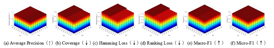
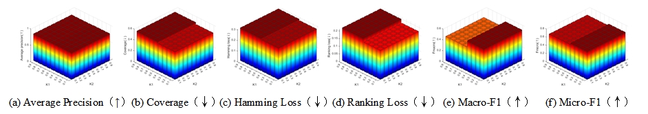
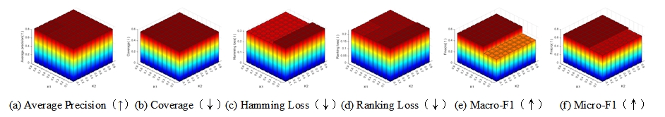
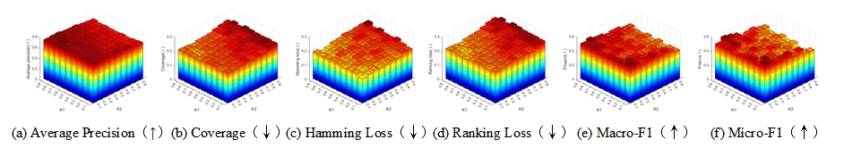
5.5 Parameter sensitivity analysis

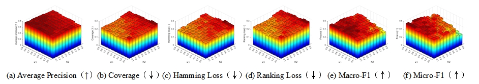
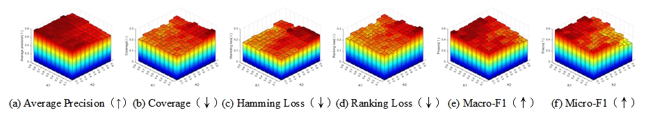
This section focuses on investigating the impact of parameters $k_{1}$ and $k_{2}$ on the FedCMFS using two datasets, Flags and Image. The analysis include diverse client numbers, with detailed outcomes presented in Figure 5 to Figure 10.

In the case of the low-dimensional Flags dataset, it was found that the parameter $k_{1}$ has a relatively small effect on the results, while $k_{2}$ has a negligible effect on the results. Specifically, when the number of clients is 3 and 5, setting $k_{1}$ in the range $\left[0.1,0.4\right]$ can obtain better experimental results. In contrast, for 10 customers, the optimal range of $k_{1}\in\left[0.4,0.9\right]$. This variation in results is attributed to the limited number of features in the Flags dataset, resulting in fewer feature bases filtered out by FedCFR and FedCFC, thus reducing the impact of $k_{1}$ and $k_{2}$. Therefore, it may be more effective to use only FedCFL and FedCFR for feature selection. In addition, the experimental results are affected by the number of clients, with an inversion of the effective parameter range at 10 clients. This variation may be caused by the uneven distribution of samples in the smaller dataset when simulating the federated environment

In the case of the high-dimensional Image dataset, the parameters $k_{1}$ and $k_{2}$ have a significant impact on the experimental results. In all three client scenarios, the results improve significantly when $k_{1}$ is set within $[0.6,0.9]$ and $k_{2}$ is set within $[0.1,0.3]$. This sensitivity is attributed to the large number of features of the dataset, which allows FedCFR and FedCFC to effectively process and screen more features due to the complex associations present in the high-dimensional data. By correcting the top 10% to 30% of possible erroneous features, FedCFR achieves the best performance. However, increasing the number of corrected features may lead to counterproductive adjustments, caused by excessive noise and strict symmetry constraints. Moreover, the complexity of the image dataset means that the data distribution is unlikely to be affected by the sampling method used to simulate the federated environment, making the number of clients irrelevant to the experimental results. The consistency of parameter sensitivities across different clients further demonstrates the effectiveness of FedCFR and FedCFC in the federated context.

Figure 5: Parameter sensitivity analysis of FedCMFS on the Flags dataset when the number of clients is 3.

Figure 6: Parameter sensitivity analysis of FedCMFS on the Flags dataset when the number of clients is 5.

Figure 7: Parameter sensitivity analysis of FedCMFS on the Flags dataset when the number of clients is 10.

Figure 8: Parameter sensitivity analysis of FedCMFS on the Image dataset when the number of clients is 3.

Figure 9: Parameter sensitivity analysis of FedCMFS on the Image dataset when the number of clients is 5.

Figure 10: Parameter sensitivity analysis of FedCMFS on the Image dataset when the number of clients is 10.

5.6 Statistical hypothesis testing

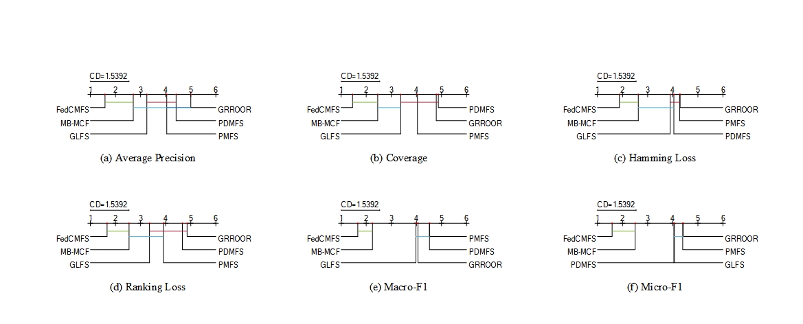
To fully establish the superiority of FedCMFS over prior methods, we conduct the Friedman test ($\alpha=0.05$) on the six metrics [36]. Table 9 shows the specific results. We observe that the Friedman statistic values on all metrics are higher than the critical value, which means the null hypothesis of no significant difference among the algorithms is rejected.

Table 9: Friedman test results.

Metric	$\mathbf{F_{F}}$	Critical Value($\alpha=0.05$)
AvP	18.2674	2.293
Cov	25.0398
HaL	9.4003
RaL	17.9430
Macro-F1	17.4678
Micro-F1	15.0658

Since rejecting the null hypothesis, we further employs the Nemenyi test [36] as a post-hoc test. The Nemenyi test indicates a significant difference in the performance of two methods if the mean rank difference between them exceed a critical difference (CD). The results are shown in Figure 11, where each rank is sequentially marked on the axis and the lowest is on the right. Notably, FedCMFS achieves the lowest rank across all metrics and significantly outperforms other methods.

Figure 11: Nemenyi Test Comparison between FedCMFS and Competitors

6 Conclusion and further work

To solve the problem of causal multi-label feature selection in the federated setting, this paper proposes the FedCMFS algorithm based on the local causal structure learning method and horizontal federated learning framework.

FedCMFS is compared with five advanced algorithms, and the results show that FedCMFS achieves the best experimental results on multiple datasets. Specifically, FedCMFS is able to directly determine the parent-child relationship of variables by mining the causal relationship between variables, thus providing excellent interpretability. Second, the FedCMFS algorithm operates in a distributed data environment and maintains data privacy during the transmission of encrypted semantics. Finally, FedCMFS is also able to effectively correct the effects of noise and differences in client data quality on algorithm performance. However, there are still issues that need to be further investigated to advance the field. We observe that FedCMFS, which is based on statistical methods, may incorrectly learn the causal relationships when the dataset is sparse, leading to incorrectly selected features, e.g., the algorithm does not perform well on extremely sparse datasets such as Yeast, Flags, etc. Therefore, exploring federated causal multi-label feature selection in sparse datasets is also a promising research direction [37].

References

- [1] M.-L. Zhang, Z.-H. Zhou, A review on multi-label learning algorithms, IEEE transactions on knowledge and data engineering 26 (8) (2013) 1819–1837.
- [2] Y. Tian, K. Bai, X. Yu, S. Zhu, Causal multi-label learning for image classification, Neural Networks 167 (2023) 626–637.
- [3] S. Kashef, H. Nezamabadi-pour, B. Nikpour, Multilabel feature selection: A comprehensive review and guiding experiments, Wiley Interdisciplinary Reviews: Data Mining and Knowledge Discovery 8 (2) (2018) e1240.
- [4] J. Li, K. Cheng, S. Wang, F. Morstatter, R. P. Trevino, J. Tang, H. Liu, Feature selection: A data perspective, ACM computing surveys (CSUR) 50 (6) (2017) 1–45.
- [5] X. Wu, B. Jiang, K. Yu, H. Chen, C. Miao, Multi-label causal feature selection, in: Proceedings of the AAAI conference on artificial intelligence, Vol. 34, 2020, pp. 6430–6437.
- [6] J. Pearl, Causality, Cambridge university press, 2009.
- [7] B. McMahan, E. Moore, D. Ramage, S. Hampson, B. A. y Arcas, Communication-efficient learning of deep networks from decentralized data, in: Artificial intelligence and statistics, PMLR, 2017, pp. 1273–1282.
- [8] Q. Yang, Y. Liu, T. Chen, Y. Tong, Federated machine learning: Concept and applications, ACM Transactions on Intelligent Systems and Technology (TIST) 10 (2) (2019) 1–19.
- [9] R. Cai, Z. Zhang, Z. Hao, Bassum: A bayesian semi-supervised method for classification feature selection, Pattern Recognition 44 (4) (2011) 811–820.
- [10] K. Yu, X. Guo, L. Liu, J. Li, H. Wang, Z. Ling, X. Wu, Causality-based feature selection: Methods and evaluations, ACM Computing Surveys (CSUR) 53 (5) (2020) 1–36.
- [11] R. B. Pereira, A. Plastino, B. Zadrozny, L. H. Merschmann, Categorizing feature selection methods for multi-label classification, Artificial intelligence review 49 (2018) 57–78.
- [12] J. Lee, D.-W. Kim, Fast multi-label feature selection based on information-theoretic feature ranking, Pattern Recognition 48 (9) (2015) 2761–2771.
- [13] J. Lee, D.-W. Kim, Scls: Multi-label feature selection based on scalable criterion for large label set, Pattern Recognition 66 (2017) 342–352.
- [14] J. Dai, W. Huang, C. Zhang, J. Liu, Multi-label feature selection by strongly relevant label gain and label mutual aid, Pattern Recognition 145 (2024) 109945.
- [15] Z. Ma, F. Nie, Y. Yang, J. R. Uijlings, N. Sebe, Web image annotation via subspace-sparsity collaborated feature selection, IEEE Transactions on Multimedia 14 (4) (2012) 1021–1030.
- [16] J. Huang, G. Li, Q. Huang, X. Wu, Joint feature selection and classification for multilabel learning, IEEE transactions on cybernetics 48 (3) (2017) 876–889.
- [17] M. Faraji, S. A. Seyedi, F. A. Tab, R. Mahmoodi, Multi-label feature selection with global and local label correlation, Expert Systems with Applications 246 (2024) 123198.
- [18] R. Huang, W. Jiang, G. Sun, Manifold-based constraint laplacian score for multi-label feature selection, Pattern Recognition Letters 112 (2018) 346–352.
- [19] Z. Cai, W. Zhu, Multi-label feature selection via feature manifold learning and sparsity regularization, International journal of machine learning and cybernetics 9 (2018) 1321–1334.
- [20] J. Zhang, Z. Luo, C. Li, C. Zhou, S. Li, Manifold regularized discriminative feature selection for multi-label learning, Pattern Recognition 95 (2019) 136–150.
- [21] Y. Fan, J. Liu, J. Tang, P. Liu, Y. Lin, Y. Du, Learning correlation information for multi-label feature selection, Pattern Recognition 145 (2024) 109899.
- [22] Y. Hu, Y. Zhang, D. Gong, X. Sun, Multi-participant federated feature selection algorithm with particle swarm optimizaiton for imbalanced data under privacy protection, IEEE Transactions on Artificial Intelligence.
- [23] S. Banerjee, E. Elmroth, M. Bhuyan, Fed-fis: A novel information-theoretic federated feature selection for learning stability, in: International Conference on Neural Information Processing, Springer, 2021, pp. 480–487.
- [24] J. Pearl, Probabilistic reasoning in intelligent systems: networks of plausible inference, Morgan kaufmann, 1988.
- [25] K. Yu, L. Liu, J. Li, A unified view of causal and non-causal feature selection, ACM Transactions on Knowledge Discovery from Data (TKDD) 15 (4) (2021) 1–46.
- [26] C. F. Aliferis, A. Statnikov, I. Tsamardinos, S. Mani, X. D. Koutsoukos, Local causal and markov blanket induction for causal discovery and feature selection for classification part i: algorithms and empirical evaluation., Journal of Machine Learning Research 11 (1).
- [27] N. Friedman, M. Linial, I. Nachman, D. Pe’er, Using bayesian networks to analyze expression data, in: Proceedings of the fourth annual international conference on Computational molecular biology, 2000, pp. 127–135.
- [28] J. Peng, P. Wang, N. Zhou, J. Zhu, Partial correlation estimation by joint sparse regression models, Journal of the American Statistical Association 104 (486) (2009) 735–746.
- [29] J. D. Owens, M. Houston, D. Luebke, S. Green, J. E. Stone, J. C. Phillips, Gpu computing, Proceedings of the IEEE 96 (5) (2008) 879–899.
- [30] J. Zhang, H. Wu, M. Jiang, J. Liu, S. Li, Y. Tang, J. Long, Group-preserving label-specific feature selection for multi-label learning, Expert Systems with Applications 213 (2023) 118861.
- [31] J. Miao, Y. Wang, Y. Cheng, F. Chen, Parallel dual-channel multi-label feature selection, Soft Computing 27 (11) (2023) 7115–7130.
- [32] J. Zhang, Y. Lin, M. Jiang, S. Li, Y. Tang, K. C. Tan, Multi-label feature selection via global relevance and redundancy optimization., in: IJCAI, 2020, pp. 2512–2518.
- [33] A. Hashemi, M. B. Dowlatshahi, H. Nezamabadi-pour, An efficient pareto-based feature selection algorithm for multi-label classification, Information Sciences 581 (2021) 428–447.
- [34] J. M. Pena, Learning gaussian graphical models of gene networks with false discovery rate control, in: European conference on evolutionary computation, machine learning and data mining in bioinformatics, Springer, 2008, pp. 165–176.
- [35] M.-L. Zhang, Z.-H. Zhou, Ml-knn: A lazy learning approach to multi-label learning, Pattern recognition 40 (7) (2007) 2038–2048.
- [36] J. Demšar, Statistical comparisons of classifiers over multiple data sets, The Journal of Machine learning research 7 (2006) 1–30.
- [37] G. Xiang, H. Wang, K. Yu, X. Guo, F. Cao, Y. Song, Bootstrap-based layer-wise refining for causal structure learning, IEEE Transactions on Artificial Intelligence.