Nonequilibrium Phase Transition in a 2D Ferromagnetic Spins with Effective Interactions

Abstract

We investigate nonequilibrium phase transitions in a 2D ferromagnetic Ising model on a square lattice with effective interactions using Monte Carlo-based computational algorithms. We verify the effective parameter $h$ by employing mean-field theory and derive self-consistent equations (SCEs) using two familiar dynamics: Metropolis and Glauber. For $-1<h<1$, both dynamics are expected to estimate the same SCE. We find the relation between $T_{c}$ and $T_{c}^{0}$ where $T_{c}$ ($T_{c}^{0}$) is the critical temperature of the model with (without) the effective interactions. Here, $T_{c}^{0}$ refers to the well-known analytical result of the equilibrium Ising model. We perform the simulations for different lattice sizes that enable us to measure physical quantities of interest. From numerical data, we determine $T_{c}$ and relevant exponents for various values of $h$ by employing finite-size scaling (FSS). We find that the FSS result of $T_{c}$, which is quite different from $T_{c}^{0}$, is in agreement with that of its analytical result, and the accuracy is good regardless of the types of model. The numerical results of the exponents are consistent with the analytical values of the equilibrium 2D Ising model, which belongs to the same universality class.

Keywords: Nnonequilibrium Steady State, Phase Transition, Ferromagnetic Ising Model, Spin Interactions, Metropolis, Monte Carlo, Critical Exponents

1 Introduction

In equilibrium systems, the fundamental principles and standard theory of the critical behavior at/near continuous PTs are currently well understood [1, 2, 3, 4]. Ongoing research and exploration have, however, continuously focused on the investigation of PTs between nonequilibrium statistical states [5, 6, 7, 8, 9, 13, 10, 11, 12, 14, 15, 16, 17]. Despite considerable efforts, research problems associated with the classification of nonequilibrium PTs are still not completely solved. In this paper, we will address the issue of nonequilibrium PT in ferromagnetic systems by using the well-established principles of contemporary concepts of PT in equilibrium systems since equilibrium and nonequilibrium critical phenomena are similar in many aspects [12]. In the equilibrium model, PT has generically represented by singularities in the free energy and its derivatives. Such singularity causes a discontinuous property of physical quantities near the critical point. The PT is phenomenologically characterized by an order parameter, which is vanishingly zero in the disordered phase and nonvanishing in the ordered phase [18, 19, 20]. Out-of-equilibrium systems exhibit a broad range of universality classes, such as “kinetic Ising models with competing dynamics” [21, 22, 23, 24, 25, 26, 27, 28, 29, 30].

Nonequilibrium PTs are a wide research area that is increasing in most situations that are intrinsically out of equilibrium, in which the standard tools of equilibrium statistical mechanics are usually not applicable. However, fundamental concepts, such as criticality and universality, have been extended to nonequilibrium prototypes. Nonequilibrium PTs can be classified into several types such as directed percolation, active matter, and self-organized criticality. These are just a few examples, there are more examples of nonequilibrium PTs. Each type of PT has its typical properties and mathematical formalism, and understanding these transitions is indispensable for studying broad fields of complex systems across multiple disciplines. Intriguingly, it is far less completely understood, although classes have of course been studied over the last decades.

Nonequilibrium PTs are an essential research field because much of their functional nature resides out-of-equilibrium, for example, quantum annealing is used for some contemporary quantum computers for which the Ising model is directly relevant. In addition to describing several magnetic systems, the Ising model can be used to examine critical behaviors in different gasses, alloys, glasses, and liquid helium mixtures [31]. The focus of this study, however, is specific to the application of the Ising model to phases and PTs in magnetic systems. More specifically, we consider a paradigmatic example of ferromagnetic phase and paramagnetic phase and the transitions between these phases and, therefore, we use the language of two-dimensional (2D) ferromagnetic spin system. Despite a lot of recent efforts on related works, the nature of nonequilibrium PTs in Ising ferromagnet with effective interactions has not yet been studied

In related paper [16], the Monte Carlo (MC) method through a modified Metropolis and a modified Glauber algorithms were proposed to study the nature of nonequilibrium PT in the 2D Ising model, including the order of the PT, as well as its universality class. More specifically, nonequilibrium PT, where the detailed balance condition (DBC) is not fulfilled and the system reaches a nonequilibrium steady state (NESS) which is not described by Boltzmann statistics, was addressed by the modified Metropolis algorithms. In the model studied there, “activity” was introduced by modifying the update rule in a way that makes the probability of occurrence of spin flips higher than that in the equilibrium 2D Ising model. The opposite case called a "persistent Ising Mode" in which spin flips are less likely to occur than in the equilibrium model was also studied. The name persistence model was used because the modified rule serves to increase the persistence time of spin configurations.

Recently [17], we implemented a supervised machine learning adaptive approach based on convolutional neural networks to predict the critical temperature of the nonequilibrium transition from paramagnetic to ferromagnetic state in 2D Ising model on a square lattice in which the MC simulation relies on that previous study [16]. Although the modified update rule was less accurate for the “persistent” regime, the agreement between the two numerical methods was remarkably excellent. However, further investigation has been hindered due to unusual of the update rule that stems from the mathematical model. To manage such a peculiar case in this present work, we propose a strategy in which an effective Hamiltonian suffices the nonequilibrium description of the mathematical model. Interestingly, the equilibrium 2D Ising model can be solved exactly [18]. This is very useful to successfully derive the exact solution (3.19) of the nonequilibrium transition temperature. We employ mean field approximation (MFA) which is the prominent method to exhibit the qualitative picture of the problem. We use the MC method [32, 33] to provide the numerical results in detail.

The rest of the sections are organized as follows: We present the model considered in this work, followed by a concise description of our methods in Section 2. Section 3 is mainly devoted to explaining the existence of effective parameters in line with the occurrence of PT using MFA by exhibiting some qualitative results. The numerical results of this study are then illustrated and discussed in Section 4 in detail. We conclude with a summary of the main finding, as provided in Section 5.

2 Methods and Model

2.1 Ferromagnetic Ising Model

We consider a 2D ferromagnetic Ising model on a square lattice of linear size $L$ comprising $V=L^{d}$ sites where $d$ denotes the number of spatial dimensions. Each site on the lattice contains a single spin pointing upwards or downwards, and the total number $N$ of spins is equal to the size of the system, $N=V$. Let a Hamiltonian describing PTs in Ising effective interactions consist of nearest-neighbor $\mathcal{H}_{0}$ and others $\mathcal{H}^{\prime}$ terms, $\mathcal{H}=\mathcal{H}_{0}+\mathcal{H}^{\prime}$ where $\mathcal{H}_{0}$ refers to the standard equilibrium Ising Hamiltonian while $\mathcal{H}^{\prime}$ in turn consists of $\mathcal{H}_{1}$ and $\mathcal{H}_{2}$ terms. By $\mathcal{H}_{1}$, we mean the interaction part other than $\mathcal{H}_{0}$. Therefore,

$$\mathcal{H}=\underbrace{-J\sum_{\langle i,j\rangle}S_{i}S_{j}}_{\mathcal{H}_{0}}-\underbrace{\underbrace{\sum_{ij^{\prime}\neq\langle ij\rangle}J_{ij^{\prime}}S_{i}S_{j^{\prime}}}_{\mathcal{H}_{1}}-\underbrace{\mathcal{B}\sum_{i}S_{i}}_{\mathcal{H}_{2}}}_{\mathrm{others}}.$$ (2.1)

where $S_{i}$ is the value of the spin variable at site $i=\{1,\cdots,N\}$ that can be either $\pm 1$(up or down), indices of sites $\langle i,j\rangle$ denotes the sum over all nearest-neighbor pairs [32, 33, 34] while $ij^{\prime}\neq\langle ij\rangle$ prompts sum over others except the nearest-neighbors while the third sum is over all $N$ sites. The statistical average of an observable $\langle\mathcal{O}\rangle$ derived from canonical partition sum $Z$ is

$$\langle\mathcal{O}\rangle=\frac{1}{Z}\sum\mathcal{O}\exp\left[-\frac{\mathcal{H}}{k_{B}T}\right]\texttt{,}$$ (2.2)

using

$$Z=\sum\exp\left[-\beta\mathcal{H}\right]\texttt{,}\mathrm{\;\;\;and\;\;\;}\beta=\frac{1}{k_{B}T}\texttt{,}$$

where $T$ is temperature and $k_{B}$ is Boltzmann constant. Classically, if distinction of the spin as an operator is not required, the total energy of the Ising spin model from (2.1) and (2.2) gives $E=E^{0}+E^{12}$ where $E^{0}=\langle\mathcal{H}_{0}\rangle$ and $E^{12}=\langle\mathcal{H}_{1}\rangle+\langle\mathcal{H}_{2}\rangle$. We define the nearest-neighbor equilibrium Ising energy as usual,

$$E^{0}=-J\sum_{\langle i,j\rangle}S_{i}S_{j}\texttt{.}$$ (2.3)

Let us now introduce a modified formalism, and perhaps conceptually simple approach of total energy calculation by considering all (other) interactions into account. The primary objective of this manifestation is to express $E^{12}$ in terms of $E^{0}$ (2.3) such that $E^{12}:=hE^{0}$, where $h$ is an effective parameter to be determined bearing on its qualification to establishing the model’s nonequilibrium nature(see A.1), without loss of generality. We have $E=E^{0}+E^{12}$ and $E^{12}=hE^{0}$ therefore, $E\equiv E(h)=(1+h)E^{0}$,

$$E(h)=-J(1+h)\sum_{\langle i,j\rangle}S_{i}S_{j}\texttt{,}$$ (2.4)

where $E^{0}$ can be retrieved with $h=0$. We emphasize that the term $J(1+h)$ in energy function (2.4) does not replace the exchange parameter $J$ of the equilibrium model (2.3). Rather, depending on the choice of $h$ that determines the stochastic dynamical behavior, this term may describe a nonequilibrium model, as will become clearer later (see Section 3 and A.1). Henceforward, we use $E^{0}=E(h=0)$ to represent the equilibrium Ising energy given in  Eq. (2.3), and $E=E(h\neq 0)$ represent the nonequilibrium Ising energy for the sake of simplicity. We also keep this notation consistent for others such as temperature $T^{0}=T(h=0)$ and $T=T(h\neq 0)$. Note that the unit of the temperature is related to that of $J/k_{B}$ where the ferromagnetic energy scale $J>0$ stands for the coupling strength of each spin to its nearest-neighbors. To simplify the notation, we will now set $k_{B}=1$, hence $T:=T/J$ is dimensionless.

Based on the postulates of equilibrium ($h=0$) statistical physics for the system in contact with a heat bath (thermal reservoir) at a temperature, each of the spin configurations $\{S\}$ happens with a probability $\mathcal{P}^{0}\propto\exp[-\beta^{0}E_{\{S\}}^{0}]$. The transition temperature of the equilibrium Ising model with $d-$number of spatial dimensions was derived [18] to be

$$T_{c}^{0}=\frac{zJ}{2\ln(1+\sqrt{2})},$$ (2.5)

where $z=2d$ represents the possible number of the nearest-neighbor spins. We aim to test and show how also this trend works for the case $h\neq 0$. At this point, it is natural to ask some questions: (i) What choice of the effective parameter $h$ determines the stochastic dynamical behavior? In other words: How does changing the values of $h$ affect the stochastic dynamical system? (ii) Does this also affect the nature of PT and its transition temperature $T_{c}$ different from (2.5)? If so, how is it changing with changing $h$, and how do we determine this $T_{c}$? In fact, we argue that the postulates is applicable also in the case of $h\neq 0$ for those values of $h$ in which the equilibrium condition holds for dynamic processes approaching thermal equilibrium. Here, stochastic dynamical processes play a crucial role in the equilibrium models, such as $N$-particle systems in contact with the heat bath at $T=T(h)$. At a limit of an asymptotically long time, this system approaches a statistically stationary state in which it gets through certain configuration $\{S\}$ according to a well-defined probability distribution . An explicit form of the above partition sum $Z=Z_{N}(h)$ is now given as

$$Z=\sum_{\{S\}}\exp[-\beta E_{\{S\}}]\equiv\sum_{\{S\}}\exp\left[-(1+h)\beta E_{\{S\}}^{0}\right],$$

where $E^{0}$ is from Eq. (2.3) and the sum runs over all possible $\{S\}$ configurations. Consequently, the effective $Z$ reads

$$Z\equiv\sum_{\{S\}}\left(\exp\left[-\beta E^{0}\right]\frac{}{}\right)^{(1+h)}=\sum_{\{S\}}\left(g\frac{}{}\right)^{(1+h)},$$ (2.6)

where $g=\exp\left[-\beta E^{0}\right]$ is the well known Gibs-Boltzmann distribution. Certain macroscopic quantities of interest can be derived from Eq. (2.6). Here, the system encounters a second order PT at temperature $T_{c}=T_{c}(h)$, and we will show that this is true for $-1<h<1$. For a value of $h$ in this range, the transition temperature is quite different from that of the transition for $h=0$, $T_{c}(|h|<1)\neq T_{c}^{0}$. The system magnetizes for $T<T_{c}$ where the resulting state is ferromagnetic or the ordered state. The system is in a disordered (or paramagnetic) state for $T>T_{c}$. The order parameter is usually given by average magnetization per site $\langle M\rangle/N$ where

$$M\equiv M(h)=\left|\sum_{i}S_{i}\right|\texttt{,}$$ (2.7)

and it quantitatively distinguishes the two phases realized by the system. That is, one can use Eq. (2.7) to describe how ordered the system is, where zero $\langle M\rangle/N$ refers to the state in which the orientation of spins is disordered and non-zero $\langle M\rangle/N$ corresponds to the state in which it is in a preferred direction. Determining $T_{c}$ and analyzing the nature of transition will be competent tasks of this paper. Primarily, however, we should have to appropriately prove and justify the existence of an effective parameter $h$.

2.2 Monte Carlo simulation method

Consider a system that generates stochastic spin flips when in contact with a thermal reservoir [35]. In the equilibrium Ising model, the system achieves thermal equilibrium after a sufficiently long time, and the description of the steady-state distribution is subject to the Boltzmann distribution. This permits one to define transition rates and calculate the flipping probabilities. Nonequilibrium PT is discussed with emphasis on general features such as the role of breaking DBC in generating effective interactions [36]. In principle, DBC can be sufficient$-$but it is not necessary to ensure equilibration. For this work, our model violates the DBC and causes the system to come out of equilibrium based on the nature of the effective interaction in consideration ($h\neq 0$). In agreement with the discussion in related work [16], there is a situation in which the system shows a disorder-order transition that is not similar to the usual equilibrium PT. As each spin flips from time to time due to the influence of thermal fluctuation, we use the master equation (ME) to develop this idea in terms of stochastic changes in its configurations. The intrinsic stochastic dynamics of the system allow us to compute its thermodynamic properties. In fact, most of our knowledge about equilibrium PT can be extended to the nonequilibrium case as well.

Denoting the spin configuration before the flip $\texttt{b}=\{S_{1},...,\pm S_{i},...,S_{N}\}$, the system’s state is described according to probability theory that the state has a configuration b at time $t$, with probability $\mathcal{P}_{b}(h,t)$. There are $2^{N}$ total configurations$-$thus we have an absolute stochastic form of the state at time $t$ if we can describe all the $2^{N}$ values of $\mathcal{P}_{b}(h,t)$ for each $b$s. The ME justifies how such a set of probabilities evolves with $t$. Assuming that the configuration after the flip will be $\texttt{a}=\{S_{1},...,\mp S_{i},...,S_{N}\}$, the transition changes from state b to a with rate of transition probability $W(b\rightarrow a)$ in a couple of time interval $\Delta t$ [34]. Consequently, the probability that the configuration of system being in state b decreases by $W(b\rightarrow a)\Delta t\mathcal{P}_{b}(h,t)$, since the system was in b with probability $\mathcal{P}_{b}(h,t)$ and then has changed to a with rate of transition probability $W(b\rightarrow a)$ in interval $\Delta t$. Correspondingly, the probability that it is in state b would be increased by $W(a\rightarrow b)\Delta t\mathcal{P}_{a}(h,t)$. The ME is basically a linear partial differential equation determining probability fluxes (net flow away from and into a configuration). We shall use a discrete form of ME, as it is for the implementation of MC simulation in mind, and define the net change of probability per small time interval $\Delta t$ as follows:

$$\frac{\Delta\mathcal{P}_{b}(h,t)}{\Delta t}=\sum_{a\neq b}W(a\rightarrow b)\mathcal{P}_{a}(h,t)-\sum_{a\neq b}W(b\rightarrow a)\mathcal{P}_{b}(h,t),$$ (2.8)

where $\Delta\mathcal{P}_{b}(h,t)=\mathcal{P}_{b}(h,t+\Delta t)-\mathcal{P}_{b}(h,t)$. This ME (2.8) is an implicit idea of Markov processes where the characteristic change of $\mathcal{P}_{b}(h,t)$ is completely described as an effective probability distribution at time $t$ while $h$ is fixed. Though a proposition that the dynamics are generated by heat baths secures that the rates (2.8) satisfy DB at some control parameters, we intended to deal with rates violating DB. In sufficiently long-time limit $t\to\infty$, a stochastic dynamical system approaches a statistically stationary state where it evolves through certain configuration according to a distinct probability distribution that does not change with time and $\Delta\mathcal{P}_{b}(h,t\to\infty)\approx 0$. The key advantage of this concept is the appearance of a Hamiltonian (2.1) relating each state of configuration $\{S\}$ with a certain effective energy (2.4). The ME is reduced to

$$\sum_{a\neq b}W(b\rightarrow a)\mathcal{P}_{b}(h)=\sum_{a\neq b}W(a\rightarrow b)\mathcal{P}_{a}(h),$$ (2.9)

which we refer to as global DBC for dynamical systems approaching thermal equilibrium. The global condition (2.9) requires a local condition,

$$W(b\rightarrow a)\mathcal{P}_{b}(h)=W(a\rightarrow b)\mathcal{P}_{a}(h)\texttt{.}$$ (2.10)

For $h=0$, the ratio of the transition rates (or probabilities) is equal to the Boltzmann weighting, $r(h=0)\equiv{\mathcal{P}_{a}}/{\mathcal{P}_{b}}=\mathrm{e}^{-\beta\Delta E^{0}}$, and it only specifies the ratio of weights but not their values. However, an intrinsic microscopic irreversibility will essentially produce macroscopic nonequilibrium properties and we intended to study nonequilibrium PT occurring due to violation of local DB. As a matter of fact, the distribution of stochastic dynamical approaching thermal equilibrium may not necessarily be the Gibbs-Boltzmann distribution [34]. Hence it will be customary for $h\neq 0$ to choose an appropriate weight in MC simulations that $\mathcal{P}_{b,a}(h)=\frac{1}{Z}\exp[-\beta E_{b,a}(h)]$ to get the ratio

$$r(h)=\mathrm{e}^{-\beta\Delta E}.$$ (2.11)

where $\Delta E=E_{\texttt{a}}(h)-E_{\texttt{b}}(h)$ is the energy change due to the transition from a present state b("before the flip") to a new state a("after the flip"). Using Eq. (2.4),

$$\Delta E=J(1+h)\sum\left(S_{i}^{\texttt{b}}-S_{i}^{\texttt{a}}\right)S_{j}=2J(1+h)S_{i}\sum_{j}S_{j}\texttt{,}$$

where the spin $S_{i}$ before and after the flip has opposite sign ($S_{i}^{\texttt{b}}=-S_{i}^{\texttt{a}}\equiv S_{i}$), while the nearest neighbors remain the same ($S_{j}^{\texttt{a}}=S_{j}^{\texttt{b}}\equiv S_{j}$). Here, $S_{j}$ represents the possible $z$ nearest neighbors of the $i^{\texttt{th}}$ site. Therefore, the effective change in energy becomes

$$\Delta E=(1+h)\Delta E^{0}\texttt{,}$$ (2.12)

where $\Delta E^{0}$ is defined as

$$\Delta E^{0}=2JS_{i}\sum_{j}S_{j}\texttt{,}$$ (2.13)

with $-\Delta E_{\texttt{max}}^{0}\leq\Delta E^{0}\leq\Delta E_{\texttt{max}}^{0}$. Using a simple version of the Ising (spin $1/2$) like Hamiltonian [37] described in Eq. (2.1) in which $\left\langle i,j\right\rangle$ refers to the sum over $z$ nearest neighbors, $\Delta E_{\texttt{max}}^{0}=2zJ$ where each spin is linked to other $z$ neighbors. The ratio (2.11) along with Eq. (2.12) can be used to describe the two most commonly used transition rates namely the Metropolis [38] update rule

$$W=\texttt{MIN}\left[1,\exp\left[-\beta\Delta E\right]\frac{}{}\right]\texttt{,}$$ (2.14)

and the Glauber [39, 40, 41] update rule

$$W=\frac{1}{2}\left(1-\tanh\left[\frac{\beta\Delta E}{2}\right]\right)\texttt{.}$$ (2.15)

We will modify these update rules (2.14) and (2.15) to intentionally break the DBC assuming that the sign of $h$ in Eq. (2.12) does not change with that of $\Delta E^{0}$,

$$h\Delta E^{0}=h|\Delta E^{0}|\texttt{,}$$ (2.16)

where $-1<h<1$ is the effective parameter and $\Delta E^{0}$ is readily found from (2.13). Remarkably, the usual form of both algorithms (which respect the DBC) can be retrieved if we set $h=0$. For a square lattice Ising in equilibrium ($h=0$), we have $z=4$ and $\Delta E^{0}$ can take a set of values $\Delta E^{0}=\{-8,-4,0,4,8\}$.

For results reported in Section 4, we manage the simulation of the model system specified by Eq. (2.4) on a square lattice of linear size $L$ applying periodic boundary condition in each direction. We start the simulations from the high value of $T$ in the range and set an initial state to be random configurations. The Markov process is governed by a single spin dynamics of the (effective) Metropolis algorithm (2.14). The dynamics is determined with $\Delta E$ (2.12) keeping the restriction (2.16) and calculate an actual energy difference as,

$$\Delta E=2S_{i}\sum_{j}S_{j}+2h\left|\sum S_{j}\right|\texttt{.}$$ (2.17)

Replacing $\Delta E$ in the update rule (2.14) by this modified version (2.17), we find that the modified Metropolis update rule conveniently breaks the DBC. Meaningfully, we compute the actual energy update using Eq. (2.4) without the restriction given (2.16). For each $T$ in the temperature list and a specified value of $h$, we choose a random site $i$ of spin $S_{i}$ from $L\times L$ lattice.

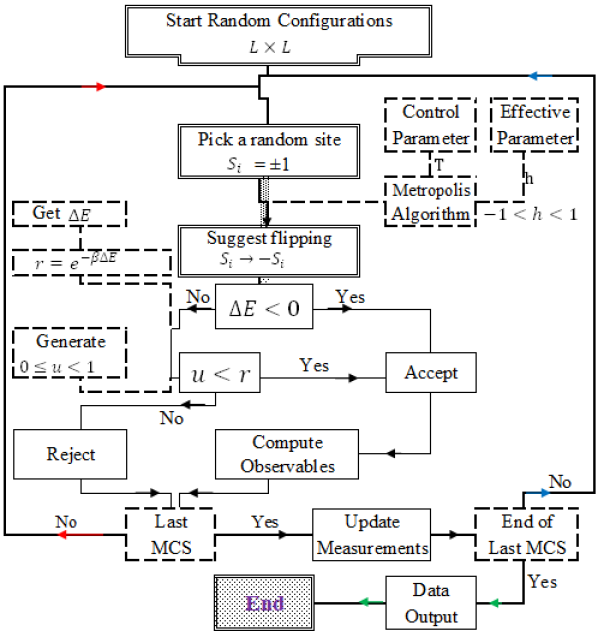
Figure 1: Schematic flow chart of the (modified) Metropolis algorithm (2.14) using $\Delta E$ given in Eq. (2.17).

The flow chart (Figure 1) summarizes the modified Metropolis algorithm which is the update rule to be implemented in this work. The basics of the flow chart are as follows. Suggest a transition from $S_{i}=\pm 1$ to $S_{i}=\mp 1$ and always accept the transition if it lowers the energy. If it raises the energy, accept the transition with a certain probability which requires to compute $r$ with Eq. (2.11). Then generate a random number $u$ distributed uniformly between $0\leq u<1$ and accept the transition if $u<r$. If $r>1$, it is actually unnecessary to bother generating $u$. This process would be repeated for $N$ sweeps as a MC step (MCS) per site where we discard the first $10^{5}$ MCS per site to allow it to attain NESS for all systems. Then again, we measure the averaged quantities of interest in completing more $10^{5}$ MCS per site. The average over the representatives is done using 100 independent measurements.

3 Phase Transitions and Effective Parameter Explained

This section is devoted mainly to explaining the existence of effective parameter $h$ and its verification with the occurrence of phase transition (PT). We treat the solution of the model in consideration using the mean-field (MF), also known as the Curie-Weiss molecular field approximation. In the context of this paper (and previous work), the occurrence of nonequilibrium PT solely relies on the existence of a parameter violating DBC. We discuss the computational algorithm under MF approximation (MFA) based on both Metropolis (2.14) and Glauber (2.15) dynamics to derive self-consistent equations (SCEs), and demonstrate the results quantitatively and qualitatively. Even though MF prediction is quantitatively not correct, the model’s qualitative behavior is outstandingly identical to the standard solution. In adopting and establishing nonequilibrium PTs, the effective values of parameter $h$ must be determined and explained. If $h$ exists and its value prescribes the violation of DBC, the transition should be regarded as nonequilibrium PT. Therefore, identifying and prescribing this parameter is very useful for actually describing the occurrence of PT, and also for the presentation and validation of the main results in Section 4.

3.1 Verification of effective parameter with MFA

In order to treat the general form of Hamiltonian (2.1) in MFA, we may begin with defining each spin in spin interaction terms as $S_{i}=\langle S_{i}\rangle+\triangle S_{i}$ where $\triangle S_{i}=S_{i}-\langle S_{i}\rangle$ refers to the fluctuations about the mean value of $S_{i}$ and the thermal average $\bar{m}\equiv\langle S_{i}\rangle$. In MFA we assume that each spin interacts with a kind of magnetic cloud [42] described by the mean magnetization. This means that MF estimates that each spin $S_{i}$ interacts with the effective field arising intrinsically from its interaction with all the neighboring spins. Contextually, the long-range regime of MFA has been examined in respective models [43]. The application of MC simulations to the MF Ising model has been also shown [44, 45]. In the equilibrium case, the dynamics of the system satisfy DBC. To establish the nonequilibrium properties, we choose an effective parameter $h$ as a prescription for the dynamics that violets DBC.

3.1.1 Metropolis dynamics:

Considering approximate schemes for accounting the interactions between particles (spins in this case), let us begin with the Metropolis dynamics of a single spin flip, $S_{i}\to-S_{i}$:

$$w=\texttt{MIN}\left[1,\exp\left[-\beta\Delta E\right]\right]\texttt{,}$$ (3.1)

where $\Delta E=\Delta E(\textsc{MF})$ is the energy difference due to the flip of spin $S_{i}$ and $\beta=1/T$ denotes the inverse of temperature $T(h)$. This is similar to Eq. (2.14) but here we use the MF formalism of $\Delta E$ in which $\Delta E^{0}:=2Jz\bar{m}S_{i}$, where $z=2d$ represents the possible number of neighbors for a given $d$-number of spatial dimensions. It follows that

$$\Delta E=2Jz\bar{m}(1+h)S_{i}\texttt{.}$$ (3.2)

Previously as introduced in Section 2, the modified version of the energy difference would be convenient to describe the stochastic dynamical system that breaks the DBC. Straightforward from Eq. (2.17), this compatibility requires that

$$\Delta E=2Jz\bar{m}(S_{i}+h)\texttt{,}$$ (3.3)

and substitute this (3.3) in (3.1) to get the MF rate of transition for Metropolis dynamics

$$w=\left\{\begin{array}[]{ll}\exp\left[-2\beta Jz\bar{m}(S_{i}+h)\right],&\hbox{}\Delta E\mathrm{\eqref{Eq:3.03}}>0;\\ 1,&\hbox{otherwise.}\end{array}\right.$$ (3.4)

Incorporating this MFA, let us now describe a SCE for $\bar{m}$ and so it will be solved numerically. Let the spin variable at site $i$ is $S_{i}=\{S_{\bullet},S_{\circ}\}$ where $S_{\bullet}=1$ and $S_{\circ}=-1$. Thus $w_{\bullet\rightarrow\circ}$ denotes the probability of flipping from $S_{\bullet}$ to $S_{\circ}$ and, similarly, $w_{\circ\rightarrow\bullet}$ denotes the probability of flipping from $S_{\circ}$ to $S_{\bullet}$ in the steady state of the system. Defining $r$ as the ratio (2.11) of these probabilities, which is a function of $\beta$, $m$, and $h$, it can be simplified as

$$r(\beta,\bar{m},h)=\frac{w_{\bullet\rightarrow\circ}}{w_{\circ\rightarrow\bullet}}\equiv\frac{\mathcal{P}_{\circ}}{\mathcal{P}_{\bullet}}\texttt{.}$$ (3.5)

Consequently, we can express MF magnetization $\bar{m}$ in terms of ratio $r$ to get the required SCE,

$$\bar{m}(h)=\frac{1}{Z}\sum_{\{s\}=\pm 1}\mathcal{P}_{\{s\}}S_{i}\texttt{,}\mathrm{\;where\;\;}Z=\mathrm{e}^{-\beta E_{\bullet}}+\mathrm{e}^{-\beta E_{\circ}}\texttt{,}$$

$$\bar{m}(h)=\frac{1-r(\beta,\bar{m},h)}{1+r(\beta,\bar{m},h)}\texttt{.}$$ (3.6)

This SCE can be solved merely for some values of $h$ for which the DBC is satisfied. Proceeding with equilibrium dynamics ($h=0$), $r(\beta,\bar{m},h=0)=\exp[-2\beta^{0}Jz\bar{m}]$ where here $\beta^{0}=\beta^{0}(\textsc{MF})$ denotes $1/T(h=0)$. Consequently

$$\bar{m}(h=0)=\frac{1-\exp[-2\beta^{0}Jz\bar{m}]}{1+\exp[-2\beta^{0}Jz\bar{m}]},$$

$$\bar{m}(h=0)=\tanh[\beta^{0}Jz\bar{m}]\texttt{ (Equilibrium SCE), }$$ (3.7)

which is the well-known SCE for the magnetization and we refer to this (3.7) as original SCE of the equilibrium Ising model.

Given the modified MF version of $\Delta E$(3.3), it is important to sort the following two statements: (i) If $\Delta E$ is always nonnegative, then $r=\exp[-4\beta Jz\bar{m}]$. Equation (3.6), therefore, satisfies a SCE of MF magnetization

$$\bar{m}(h\neq 0)=\frac{1-r}{1+r}=\tanh[2\beta Jz\bar{m}]\texttt{,}$$ (3.8)

which is independent of $h$. (ii) If $\Delta E$ is always non-positive, the ratio $r=1$ and therefore it turn outs that

$$\bar{m}(h\neq 0)=0\texttt{.}$$ (3.9)

In contrast, the purpose of this paper is mainly intended to the case of $h$-dependent SCE where imposing the constraint $-1<h<1$ implicitly admits establishing a microscopic irreversibility of the dynamics. This idea will be more clear in the following brief specification.

First consider the case for $\bar{m}<0$, and assume that $h$ can take any real values (the restriction $-1<h<1$ holds later). The dynamics defined in Eq. (3.4) now takes its explicit forms:

$$w_{\bullet\rightarrow\circ}^{(\bar{m}<0)}=\left\{\begin{array}[]{ll}\exp\left[-\beta(2Jz\bar{m}(1+h))\right],&\hbox{if }h<-1;\\ 1,&\hbox{if }h\geq-1\end{array}\texttt{,}\right.$$

and

$$w_{\circ\rightarrow\bullet}^{(\bar{m}<0)}=\left\{\begin{array}[]{ll}\exp\left[-\beta(-2Jz\bar{m}(1-h))\right],&\hbox{if }h<1;\\ 1,&\hbox{if }h\geq 1\end{array}\texttt{.}\right.$$

Looking for $h<-1$, this gives the ratio $r=\exp\left[-4\beta Jz\bar{m}\right]$ and the next SCE for $\bar{m}$:

$$\bar{m}(h<-1)=\frac{1-r}{1+r}=\tanh\left[2\beta Jz\bar{m}\right]\texttt{.}$$ (3.10)

One may refer this (3.10) as a SCE model for $h<-1$ though this is not of interest here. But for $h>1$, $r=1$ and $\bar{m}(h>1)=0$, indicating the negative $\bar{m}(h>1)$ has no SCE. For $-1<h<1$, we get the ratio $r=\exp\left[-2\beta Jz\bar{m}(1-h)\right]$ and this gives

$$\bar{m}(-1<h<1)=\tanh\left[\beta Jz\bar{m}(1-h)\right]\texttt{.}$$ (3.11)

Second consider the case $\bar{m}\geq 0$ in which is the transition probabilities would be,

$$w_{\bullet\rightarrow\circ}^{(\bar{m}\geq 0)}=\left\{\begin{array}[]{ll}\exp\left[-\beta(2Jz\bar{m}(1+h))\right],&\hbox{if }h>-1;\\ 1,&\hbox{if }h\leq-1\texttt{,}\end{array}\right.$$

and

$$w_{\circ\rightarrow\bullet}^{(\bar{m}\geq 0)}=\left\{\begin{array}[]{ll}\exp\left[-\beta(-2Jz\bar{m}(1-h))\right],&\hbox{if }h>1;\\ 1,&\hbox{if }h\leq 1\texttt{.}\end{array}\right.$$

For $h>1$, the ratio becomes $r=\exp\left[-4\beta Jzm\right]$ and we get the following SCE for $\bar{m}$:

$$\bar{m}(h>1)=\frac{1-r}{1+r}=\tanh\left[2\beta Jz\bar{m}\right]\texttt{,}$$ (3.12)

which is identical to the SCE (3.10). This means that the magnitude of $\bar{m}(h<-1)$ and that of $\bar{m}(h>1)$ are the same, and $\bar{m}(|h|>1)$ is independent of the parameter $h$. Comparing SCE (3.12) with SCE (3.7), for $h>1$, one can find the relation $2\beta_{c}=\beta_{c}^{0}$ as long as $\bar{m}$ is the same at critical. Hence, the critical temperature $T_{c}(h>1)\textsc{MF}=2T_{c}^{0}(\textsc{MF})$ is the same for all $h>1$ hence the PT is continuous as in the case of the equilibrium transitions. Intriguingly, we find $r=\exp\left[-2\beta Jz\bar{m}(1+h)\right]$ for $-1<h<1$, and

$$\bar{m}(-1<h<1)=\tanh\left[\beta Jz\bar{m}(1+h)\right]\texttt{.}$$ (3.13)

Note from SCE (3.11) that its MF solution must obey $\bar{m}(T,h)=-\bar{m}(T,-h)$ and hence $\tanh\left[\beta Jz\bar{m}(1-h)\right]=-\tanh\left[\beta Jz\bar{m}(1+h)\right]$. On the other hand, both $w_{\bullet\rightarrow\circ}$ and $w_{\circ\rightarrow\bullet}$ are equal to one and there is no SCE for $h\leq-1$ where $\bar{m}(h\leq-1)=0$.

It has been noticed from SCEs (3.10) and (3.12) that $\bar{m}(|h|>1)$ is independent of $h$. For the purpose of this paper, therefore, we proceed working with SCE (3.13) and compute $\bar{m}=\bar{m}(-1<h<1)$ in the form of,

$$\bar{m}=\tanh[\beta Jz|\bar{m}|(1+h)],\texttt{(Metropolis SCE).}$$ (3.14)

Amazingly, the same SCE (3.14) can be obtained also using $\Delta E$ (3.2) which means that the two different forms of $\Delta E$ give the same results for $-1<h<1$.

3.1.2 Glauber dynamics:

The update rule that introduced in Eq. (2.15) is also of theoretical interest. To go any further, we expect that Glauber SCE should be the same as that of the Metropolis SCE for both $\Delta E$(3.2) and $\Delta E$(3.3). Make use of the former (3.2) now we can easily solve the Glauber algorithm with a dynamics of single spin flip $S_{i}\rightarrow-S_{i}$ as

$$w=\frac{1}{2}\left(1-S_{i}\tanh[\beta Jz\bar{m}(1+h)]\frac{}{}\right)\texttt{.}$$ (3.15)

This result holds true also for $\Delta E$(3.3) luckily due to the fact that $\tanh(a-b)=-\tanh(b-a)$ and, therefore, $\tanh(S_{i}+h)=S_{i}\tanh(1+h)$ with $S_{i}=\pm 1$. Straightforward to the Metropolis dynamics, this Glauber dynamics gives $w_{\bullet\rightarrow\circ}=\frac{1}{2}\left(1-\tanh[\beta Jz\bar{m}(1+h)]\right)$, and $w_{\circ\rightarrow\bullet}=\frac{1}{2}\left(1+\tanh[\beta Jz\bar{m}(1+h)]\right)$. The ratio (3.5) now becomes

$$r(\beta,\bar{m},h)=\frac{1-\tanh[\beta Jz\bar{m}(1+h)]}{1+\tanh[\beta Jz\bar{m}(1+h)]},$$

thus, one can find $\bar{m}$ as in Eq. (3.6) providing a Glauber SCE: $\bar{m}(h)=\tanh[\beta Jz\bar{m}(1+h)]$. As expected, the Glauber SCE is the same as the Metropolis SCE (3.14) in the vicinity $-1<h<1$ where the DBC does not hold. The DBC holds for $h=0$ where $\bar{m}(h=0)=\tanh[\beta^{0}Jz\bar{m}]$, and for $h=1$ where $\bar{m}(h=1)=\tanh[2\beta Jz\bar{m}]$. In practice, numerically the modified form of energy difference for both dynamics is therefore,

$$\Delta E=\left\{\begin{array}[]{ll}2Jz\bar{m}(S_{i}+h),&\hbox{ if }-1\leq h\leq 1;\\ 4Jz\bar{m}S_{i},&\hbox{ if }|h|>1\texttt{,}\end{array}\right.$$ (3.16)

with the corresponding definition of magnetization SCEs (3.14).

3.1.3 Qualitative demonstration:

The MF results (3.14) and (3.16) help to derive the transition temperature $T_{c}(h\neq 0)$ using the commonly known $T_{c}(h=0)$ of the model in MF picture which can be also extended to explicitly determine the exact form of $T_{c}$ which will be useful for the verification of our standard MC calculation in Section 4. Though both dynamics can provide the same result, to make the discussion be specific, we prefer working with the Metropolis rule. For $h=0$, SCE (3.14) yields a similar result of $\bar{m}(h=0)=\tanh[\beta^{0}Jz\bar{m}]$ as in equilibrium SCE (3.7). If we consider two arbitrary values of $\beta$ at which $\bar{m}(h\neq 0)=\bar{m}(h=0)$, it follows that $\tanh[\beta Jz|\bar{m}|(1+h)]=\tanh[\beta^{0}Jz|\bar{m}|]$. This MFA gives $(1+h)\beta(\textsc{MF})=\beta^{0}(\textsc{MF})$ and

$$T(\textsc{MF})=(1+h)T^{0}(\textsc{MF}).$$ (3.17)

In particular, and remarkably, $\bar{m}(h\neq 0)$ and $\bar{m}(h=0)$ are equal at critical point, $\bar{m}(T_{c},h\neq 0)=\bar{m}(T_{c},h=0)$. Consequently, it becomes

$$T_{c}(\textsc{MF})=zJ(1+h).$$ (3.18)

Here, it is straightforward to determine $T_{c}^{0}(\textsc{MF})=Jz$ where $z=2d$ for a given number of spatial dimensions $d$. For example, $T_{c}^{0}(\textsc{MF})$ is equal to $4J$ for $d=2$, and $6J$ for $d=3$ (see Figure 2) with $J=1$ for this work. Results obtained from numerical solutions for $z=4$ and $z=6$ are shown in Figure 2 which are plots of the Metropolis-MF magnetization in SCE (3.14) versus the temperature ($\bar{m}$ vs $T$) for various values of $h$.

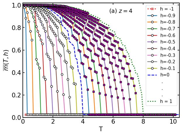
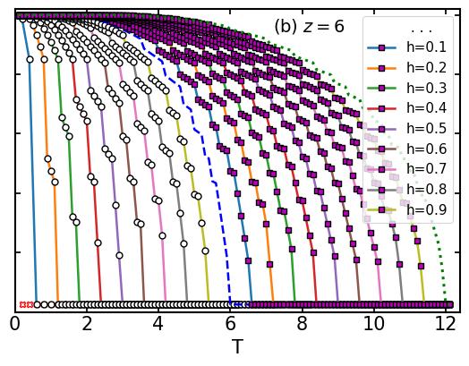
Figure 2: MF solution of magnetization per site $\bar{m}$ versus temperature $T$ for different values of $h$ (see keys). A numerical calculation of the Metropolis dynamics (3.14) for $z=2d$, (a) $d=2$ and (b) $d=3$. The dashed blue line refers to $T_{c}(h=0)=z$ and $T_{c}(h=1)=2z$ is shown by dotted line.

For $h=0$, the MF critical is $T_{c}^{0}=z$ as we expect. For $h>0$, $T_{c}$ increases with increasing $h$ and approaches $2z$ as $h\rightarrow 1$. For $h<0$, $T_{c}$ decreases with decreasing $h$ where $T_{c}\to 0$ as $h\rightarrow-1$. Specifically, at critical temperature, the figure verifies the results in Eq. (3.18) that $\bar{m}(T_{c},h)\approx 0$ for all $h$. The MFA for the model with given $z$ is therefore described as follows: For $T>T_{c}\equiv(1+h)zJ$, the system is paramagnetic (PM) with $\bar{m}=0$. For $T<T_{c}\equiv(1+h)zJ$, the system is ferromagnetic (FM) with $\bar{m}\neq 0$.

3.2 Occurrence of nonequilibrium phase transition

For the detailed numerical results Section (4), we implement the standard Metropolis algorithm as briefly introduced in Section 2. The PT should be discussed in line with the exact solution of the transition temperature $T_{c}(h)$. Here is an argument to extract the exact $T_{c}(h)$ using the result of MFA. If we replace $T_{c}^{0}$ in Eq. (3.18) with $T_{c}^{0}$ from Eq. (2.5), we get $T_{c}^{\texttt{exact}}\equiv T_{c}(h)=(1+h)T_{c}^{0}$. The exact form of the transition temperature as a function of $h$ for a given $z$ is therefore

$$T_{c}(h)=\frac{zJ(1+h)}{2\ln(1+\sqrt{2})}\texttt{.}$$ (3.19)

The simple method and direct solution of this result (3.19) has been given in A.1 (also more detail in [46]). In this sprit, Figure 2 recasts that the transition temperature would be $0\leq T_{c}(h)\leq 2T_{c}^{0}$, satisfying

$$T_{c}(h):=\left\{\begin{array}[]{ll}0<T_{c}(h)<T_{c}^{0}&\hbox{for }-1<h<0;\\ T_{c}^{0}<T_{c}(h)<2T_{c}^{0}&\hbox{for }0<h<1,\end{array}\right.$$ (3.20)

where $2T_{c}^{0}=zJ/\ln(1+\sqrt{2})$. For the fate of Section 4, we will be specific working with $z=4$ and $T_{c}(h)={2J(1+h)}/{\ln(1+\sqrt{2})}$ with $T_{c}^{0}=2J/\ln(1+\sqrt{2})\approx 2.2692$ and $2T_{c}^{0}\approx 4.5384$ are used. Dividing $T_{c}$ (3.19) to $T_{c}^{0}$ (2.5) and expressing this ratio as $k=T_{c}/T_{c}^{0}$, one can find an essential relation $k=1+h$. Thus, an alternative form of Eq. (3.20) may be defined as

$$k_{c}(h):=\left\{\begin{array}[]{ll}0<k<1&\hbox{for }-1<h<0;\\ 1<k<2&\hbox{for }0<h<1,\end{array}\right.$$ (3.21)

which reflects that the transition at $k$ is independent of $z$ (or $d$). That is; $k_{c}$ depends only on $h$ and it is the same for all $z$ regardless of the lattice structure $d$. The implication of this intuition can be explained that since $k_{c}(h)$ is the same for all $z$, only the knowledge of the equilibrium transition temperature $T_{c}(z,h=0)$ is required to determine $T_{c}(z,h\neq 0)$. Prospectively, a potential advantage of this approach (3.21) can be understood from replot of Figure 2. Further, the closed-form result of magnetization $m(h=0)$ [47] can be helpful. Figure 3 displays the magnetization $m(h=0)$ versus temperature curve for the ferromagnetic system undergoing a PT at $T=T_{c}^{0}$.

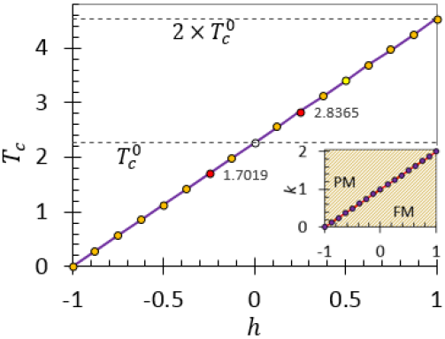
Figure 3: The transition temperature $T_{c}$ versus the parameter $h$, plot of Eq. (3.19). The horizontal dashed lines are $T_{c}(h=0)=T_{c}^{0}$ and $T_{c}(h=1)=2\times T_{c}^{0}$. For a detail numerical study, we choose $h=\pm 0.25$ where $T_{c}(h=+0.25)\approx 2.8365$ and $T_{c}(h=-0.25)\approx 1.7019$. The inset shows the ratio $k$ versus $h$ where $k=T_{c}/T_{c}^{0}$ and $T_{c}^{0}=2/\ln(1+\sqrt{2})$.

Since magnetization is a continuous quantity at $T=T_{c}^{0}$, the transition is defined to be a second-order PT. If nonequilibrium PT in the ferromagnetic Ising model appears to be in identical universality class to that of its equilibrium prototype, their critical exponents are expected to be consistent. This study is concerned with the nature of nonequilibrium transition deliberately imposing the the constraint $|h|<1$. Specifically, if we consider two $h$ values ($h=\pm 0.25$), conveniently we get that $T_{c}(h=+0.25)=5/\ln(3+2\sqrt{2})\approx 2.8365$ and $T_{c}(h=-0.25)=3/\ln(3+2\sqrt{2})\approx 1.7019$ (see Figure 3) and this is in agreement with the main results in Section 4.

4 Results and Discussion

We demonstrate the results of the MC simulation of the described model for various values of the parameter $h$ using the (modified) Metropolis algorithm, as introduced in Section 2. In the following, we briefly describe the NESS formalism of the required physical quantities, which includes magnetization, magnetic susceptibility, energy, and specific heat. Consequently, the practice of FSS analysis follows the same fashion. Then, we present some examples of the obtained numerical results and discuss them in detail.

4.1 Measurement of Physical Quantities

It has been previously argued [16] that physical quantities of interest such as the magnetization per site $m$, magnetic susceptibility $\chi$, average energy per site $\langle E\rangle/N$ and the specific-heat $C=C_{V}$ are defined in their usual forms;

$$m = \langle M\rangle/N,\mathrm{\;\;\;from\;Equation~{}\eqref{Eq:207}}\texttt{,}$$ (4.1a)

$$\chi = \left.\left(\langle M^{2}\rangle\frac{}{}-\langle M\rangle^{2}\right)\right/NT$$ (4.1b)

$$\langle E\rangle/N = \langle E\rangle\mathrm{\;per\;site\;from\;Eq.~{}\eqref{Eq:204}}\texttt{,}$$ (4.1c)

$$C = \left.\left(\langle E^{2}\rangle\frac{}{}-\langle E\rangle^{2}\right)\right/NT^{2}\texttt{.}$$ (4.1d)

Here $N=L^{2}$ is the total number of spins and the symbol $\langle\dots\rangle$ is intended to assign an average in the steady state at a given $T=T(h)$. Accordingly, the dependency of these quantities on the parameter $h$ can be tested both qualitatively and quantitatively. Making use of the modified algorithm, we perform Metropolis MC simulations of the model in consideration and measure all the required macroscopic quantities relevant to the investigation of PTs. In order to indicate the location of the transition temperature $T_{c}(h)$, we perform FSS analysis for the finite-size MC data of the Binder-cumulate $U_{4}$ associated with the distribution of the magnetization, computed as

$$U_{4}=1-\frac{\langle M^{4}\rangle}{3\langle M^{2}\rangle^{2}}\texttt{.}$$ (4.2)

Further, perusing the behavior of the system near its critical temperature is in fact a basic problem in the theory of PT. Noticeably, this behavior is well-marked as those physical quantities (4.1), and or their derivatives, possess singularities or discontinuities at the critical temperature. Here, the critical behaviors of $\chi$ and $C$ are common examples in the Ising model. In statistical physics, it is known that such singularities can be understood as a direct consequence of the fact that correlation length becomes infinitely large in the vicinity of the transition temperature. This indeed represents the correlation between spin positions in the lattice. As a result of such its infiniteness, the system becomes scale-invariance which means that the asymptotic behaviors of the relevant physical quantities near and/or at critical point are given by power laws. Continuous PTs are classified by their critical exponents, which characterize the behavior near/at the transition point. The most essential is $m\sim|T-T_{c}|^{\beta}$, $\chi\sim|T-T_{c}|^{-\gamma}$, $\xi\sim|T-T_{c}|^{-\nu}$, and $C\sim|T-T_{c}|^{-\alpha}$ where $\beta$, $\gamma$, $\nu$, $\alpha$ are critical exponents for magnetization, susceptibility, correlation length, and specific heat, respectively. For square lattice Ising model, the critical exponents $\beta=1/8$, $\gamma=7/4$, $\nu=1$, and $\alpha=0$ are known exactly. (Do not confuse the exponent $\beta$ with $1/T$. In Section 4 and 5, this symbol refers to critical exponent.)

We use FSS analysis which is convenient to examine the dependency of these quantities on $N$. For the equilibrium ($h=0$), the FSS is well known. Similarly, we treat the FSS form of quantities in NESS analogous to those quantities in thermodynamic equilibrium:

$$m \approx \mathcal{M}(1-T/T_{c})L^{(1-\beta)/\nu}\;\;\Longleftrightarrow mL^{\beta/\nu}\textsl{ vs }-\tau L^{1/\nu}$$ (4.3a)

$$\chi \approx -\mathcal{X}(1-T/T_{c})L^{(1+\gamma)/\nu}\Longleftrightarrow\chi L^{-\gamma/\nu}\textsl{ vs }\tau L^{1/\nu}$$ (4.3b)

$$C \approx -\mathcal{C}(1-T/T_{c})L^{(1+\alpha)/\nu}\Longleftrightarrow CL^{-\alpha/\nu}\textsl{ vs }\tau L^{1/\nu}\texttt{,}$$ (4.3c)

where $\mathcal{M}$, $\mathcal{X}$, $\mathcal{C}$ are their respective scaling functions and $\tau=(T-T_{c})/T_{c}$ has been used here with $\tau<0$, $\tau=0$ and $\tau>0$ for $T<T_{c}$, $T=T_{c}$ and $T>T_{c}$, respectively. For square lattice Ising model ($d=2$), the FSS relation [48, 49, 50] of the specific heat $C=C_{V}(T)$ is derived in A.2.

$\begin{array}[]{ccc}\includegraphics[width=130.08731pt]{figures/figure04a}&\includegraphics[width=130.08731pt]{figures/figure04b}&\includegraphics[width=130.08731pt]{figures/figure04c}\end{array}$

Figure 4: FSS analysis for $h=0$. (a) Binder-cumulant $U_{4}$ for different values of $L$ as a function of $T$. The intersection point provides the critical temperature $T_{c}^{\texttt{FSS}}(h=0)\approx 2.2686(4)$ and almost reconciled with $T_{c}^{0}=4/\ln(3+2\sqrt{2})$. (b)The value of maximum magnetic susceptibility $\chi^{\textsf{max}}(L)$ versus linear size $L$ in a log-log scale. (c) Maximum value of the specific heat $C^{\textsf{max}}(L)$ versus linear size $L$ while the inset shows a semi-log scale plot of the same data. The blue line is the best-fitted line to the form $\ell L^{\gamma/\nu}$ (b), $c\ln L$ (main c) and $c_{0}+c\ln L$ (inset c). Here $\ell=c/10$ was used to get $\gamma/\nu\approx 1.747\pm 0.006$ where the constant $c\approx 0.4995$ [50] and $c_{0}=c/3$.

The theory of FSS justifies how the singular properties of quantities defined in Eq. (4.1a)-$d$ near the critical point of a PT emerge when the system size becomes infinite. As usual, we use this theory from its phenomenological view of points. Therefore, we attempt to exactly demonstrate the implementation of the same FSS law in both cases ($h=0$ and $h\neq 0$). Figure 4 displays FSS analysis$-$ (a) Binder-cumulant $U_{4}$ for different values of $L$ as a function of temperature $T$ for $h=0$, and the (b) maximum value of magnetic susceptibility $\chi^{\textsf{max}}(L)$ versus linear size $L$ in a log-log scale, and (c) maximum value of the specific heat $C^{\textsf{max}}(L)$ versus linear size $L$ while the inset shows a semi-log scale plot of the same data. As we see from Figure 4, the intersection point provides the critical temperature $T_{c}^{\texttt{FSS}}(h=0)\approx 2.2686(4)$ and almost reconciled with $T_{c}^{0}=4/\ln(3+2\sqrt{2})$. The estimated values of the critical exponents are $\beta\approx 0.122\pm 0.001\equiv 0.122(1)$ and $\gamma\approx 1.747(5)$ where the exact $\nu=1$ and $\alpha=0$ (theory) were used.

4.2 Detailed Numerical Results

We now present numerical results and FSS analysis for the nonequilibrium ($-1<h<1$) model: (i) By varying the values of the parameter $h$ for a given system with fixed size $N=L^{2}$, and (ii) using a fixed value of $h$ for the system of various sizes. However, as introduced in Section 3.2, we consider $h=\pm 0.25$ for our detailed numerical results.

4.2.1 Using different $h$ values for a given system:

In the absence of an effective interaction ($h=0$), we have observed that equilibrium PT occurring at $T_{c}^{0}\approx 2.269$ as illustrated previously in Figure 4. Similarly, in the presence of effective interactions ($h\neq 0$), PTs also occur at $T_{c}(h)\neq T_{c}^{0}$. To begin with, we present in Figure 5 the plots of those physical quantities (4.1a$-$ 4.1d) as a function of $T(h)$ for various $h$ but here $L=80$ has been fixed.

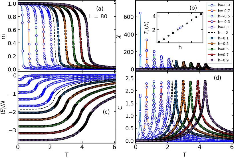
Figure 5: Plot of physical quantities (a) magnetization per spin $m$ (4.1a), (b) magnetic susceptibility $\chi$ (4.1b), (c) energy per spin $\langle E\rangle$ (4.1c) and (d) specific heat $C$ (4.1d) as a function of temperature $T$ with varying $h$ (see keys) but for fixed linear size $L=80$. For a given $h$, a peak position (panels b and d) provides an estimate of $T_{c}(h)$ where the inset within panel b is a plot of $T_{c}(h)$ versus $h$.

They all vary with varying $h$, and clearly the dashed "- -" line retrieves the equilibrium ($h=0$) quantities as expected. The peak positions of $\chi$ versus $T$ (b) and that of $C$ versus $T$ (d) give estimates of $T_{c}(h)$. In both plots (b and d), we observe the shifting of $T_{c}$ to its relatively higher values with increasing $h$. However, the position of the peaks decreases as $h$ increases with increasing $T$ for $\chi$ vs $T$ while almost unchanged for $C$ vs $T$ as expected.

4.2.2 Using a Fixed Parameter $h$ for System of Various Size

Let us proceed to analyze the critical behavior of the nonequilibrium PTs by means of FSS analysis for $h=\pm 0.25$. Figure 6 exhibits plots of physical quantities (4.1a-4.1d) as a function of temperature $T$ for (i) $h=0.25$ and (ii) $h=-0.25$ each for $L=\{30,40,60,80,120\}$.

$\begin{array}[]{cc}\texttt{(i) \;}h=0.25&\texttt{(ii) \;}h=-0.25\\ \includegraphics[width=225.48424pt]{figures/figure06a}&\includegraphics[width=225.48424pt]{figures/figure06b}\end{array}$

Figure 6: Plot of physical quantities (39) (a) $m$, (b) $\chi$, (c) $\langle E\rangle$ and (d) $C$ as a function of $T$ with varying $L$ (see keys) for each fixed parameter $h$ (i) $h=0.25$ and (ii) $h=-0.25$. In panel b and d, the vertical (orange) line represents the location of $T_{c}$ (3.19), $5/\ln(3+2\sqrt{2})\approx 2.8365$(b) and $3/\ln(3+2\sqrt{2})\approx 1.7019$(d).

In panel b and d, the vertical (orange) line represents the location of $T_{c}$ (3.19), $5/\ln(3+2\sqrt{2})\approx 2.8365$(b) and $3/\ln(3+2\sqrt{2})\approx 1.7019$(d). With increasing $L$, the maxima $\chi^{\mathrm{max}}$ and $C^{\mathrm{max}}$ clearly grow and the locations of peak points move toward the orange lines. For both $h=\pm 0.25$, all relevant properties are discussed (see Figure 7). Figure 7(a) discusses the Binder cumulant $U_{4}$ versus $T$ for various linear sizes $L$ for $h=0.25$(upper) and $h=-0.25$(lower). From the FSS relation associated with Binder (4.2), we clearly see that $U_{4}$ for various values of $L$ converge as $T\to T_{c}$ and the curves intersect at the same point. The interaction points yield a good estimation of the transition temperatures for $h=\pm 0.25$.

$\begin{array}[]{ccc}\includegraphics[width=138.76157pt]{figures/figure07hpa}&\includegraphics[width=138.76157pt]{figures/figure07hpb}&\includegraphics[width=138.76157pt]{figures/figure07hpc}\\ \includegraphics[width=138.76157pt]{figures/figure07hma}&\includegraphics[width=138.76157pt]{figures/figure07hmb}&\includegraphics[width=138.76157pt]{figures/figure07hmc}\end{array}$

Figure 7: (a) Binder cumulant $U_{4}$ computed for different values of $L$ plotted versus temperature $T$ for two values of $h=0.25$(Left) and $h=-0.25$ (Right) as shown. The intersection point provides the critical temperature $T_{c}^{\mathrm{fss}}(h)=2.8356(3)$for $h=0.25$ and $1.7012(1)$ for $h=-0.25$. (b) Plot of $\chi^{\texttt{max}}(L)$ versus $L$ in log-log scale for $h=0.25$ and $h=-0.25$. (c) Plot of $C^{\texttt{max}}(L)$ versus $L$ for $h=0.25$ and $h=-0.25$. This gives $\gamma/\nu\approx 1.748(2)$ for $h=0.25$ and $\gamma/\nu\approx 1.735(5)$ for $h=-0.25$. Note that the inset (c) shows semi-log scale for the same data of its linear scale where $C\sim c\ln L$ with $c=0.4995$ has been used.

$\begin{array}[]{c}\includegraphics[width=138.76157pt]{figures/figure08a}\includegraphics[width=112.73882pt]{figures/figure08b}\\ \includegraphics[width=138.76157pt]{figures/figure08c}\includegraphics[width=112.73882pt]{figures/figure08d}\end{array}$

Figure 8: Plot of $T_{c}^{*}(L)$ versus $1/L$ where $T_{c}^{*}(L)$ refers to the pseudo-critical point at which $\chi$(a & c) and $C$(b & d) attain their maxima. Results for $h=0.25$ (a and b) and $h=-0.25$ (c and d). The solid orange lines are the exact $T_{c}(h)$ and the dashed blue lines are $T_{c}^{\mathrm{fss}}(h=\pm 0.25)$. The solid blue lines are the best fitting line of the form Eq. (4.7). This yields (i) $T_{c}^{\mathrm{fss}}(h=0.25)\approx 2.836$ and (ii) $T_{c}^{\mathrm{fss}}(h=-0.25)\approx 1.701$, almost reconciled with $T_{c}=5/\ln(3+2\sqrt{2})$ and $T_{c}=3/\ln(3+2\sqrt{2})$.

Referring to Figure 6 (panel c), the magnetic susceptibility $\chi$ displays a peak of a size $L$-dependent transition at pseudo-critical $T_{c}^{*}(L)$. The horizontal position of the peaks shifts toward a dashed line with increasing $L$ while its vertical position increases with increasing $L$. Likewise, the specific heat $C$ (see panel d) also displays peaks that shift in agreement with that of $\chi$. If the FSS relation $\chi$ or $C$ in Eq. (4.3b) and (4.3c) peaks at certain point of value $\ell_{0}$, then the peak point $T_{c}^{*}(L)$ for a given value of $L$ changes with $L$ as

$$T_{c}^{*}(L)=\ell_{0}L^{-1/\nu}+T_{c}^{\mathrm{fss}}(h,\chi,C)\texttt{,}$$ (4.4)

where $\ell_{0}$ is a constant. On the other hand, the maximum value of the singular part of $\chi$ and $C$ in a finite-size system changes as

$$T_{c}^{*}(L)=\ell_{0}L^{-1/\nu}+T_{c}^{\mathrm{fss}}(h,\chi,C)\texttt{,}$$ (4.5)

where $\ell_{0}$ is a constant. On the other hand, the maximum value of the singular part of $\chi$ and $C$ in a finite-size system changes as

$$\chi_{L}(T=T_{c}^{*})=\chi^{\mathrm{max}}(L) \sim L^{\gamma/\nu}$$ (4.6a)

$$C_{L}(T=T_{c}^{*})=C^{\mathrm{max}}(L) \sim L^{\alpha/\nu}\texttt{,}$$ (4.6b)

and such scenarios are shown in Figure 7 (b and c). Figure 7(b) shows plots of $\chi^{\mathrm{max}}$ versus $L$ in a double log scale in which we clearly see a linear property that agrees with the power-law form of $\chi^{\mathrm{max}}$ given in (4.6a). The solid blue line is the best power-law fit that yields (i) $\gamma/\nu\approx 1.748(2)$ and (ii) $\gamma/\nu\approx 1.735(5)$. Similarly, Figure 7(c) shows a main plot of $C^{\mathrm{max}}$ versus $L$ and an inset plot on a semi-log scale for the same data. As we clearly see from the main plot, the negative curvature in data points recognizes that $C^{\mathrm{max}}$ has a weaker power-law dependence on $L$. It has been noticed from Figure 5(d) that $C^{\mathrm{max}}$ is also not sensitive to the parameter $h$ for fixed $L$. Thus it is good evidence to consider the critical exponent $\alpha\approx 0$ in the same manner as in the equilibrium (h=0) model. As a result, its plot on a semi-log scale in the inset of the main Figure (with logarithmically scaled $L$ axis) now distinctly shows a non-curvature linear property in which a blue straight line is the best fit to the form,

$$C^{\mathrm{max}}=c_{0}+c\ln L\texttt{,}$$ (4.7)

where $c_{0}\approx c/3$ is the regular part of the specific heat and $c\approx 0.4995$. In addition, we examine the validation of each of the results as shown in Figures 8 and 9. Figure 8 shows scatter plots of the peak positions $T_{c}^{*}$ versus $1/L$ as marked by $*$ symbol. Here $T_{c}^{*}(L)$ refers to the pseudo-critical point at which $\chi$(a & c) and $C$(b & d) attain their maxima. Results for $h=0.25$ (a and b) and $h=-0.25$ (c and d). The solid orange lines are the exact $T_{c}(h)$ and the dashed blue lines are $T_{c}^{\mathrm{fss}}(h)$. The solid blue lines are the best fitting line of the form $T_{c}^{*}(L)=\ell_{0}L^{-1/\nu}+T_{c}^{\mathrm{fss}}(h)$. This yields (i) $T_{c}^{\mathrm{fss}}(h)\approx 2.836$ and (ii) $T_{c}^{\mathrm{fss}}(h)\approx 1.701$, almost reconciled with $T_{c}=5/\ln(3+2\sqrt{2})$ and $T_{c}=3/\ln(3+2\sqrt{2})$.

$\begin{array}[]{c}\includegraphics[width=325.215pt]{figures/figure09a}\\ \includegraphics[width=325.215pt]{figures/figure09b}\end{array}$

Figure 9: FSS of magnetization (4.3a), susceptibility (4.3b) and specific heat (4.3c) for $h=0.25$ (upper panels) and $h=-0.25$ (lower panels). Plots of (a) $mL^{\beta/\nu}$ vs $-\tau L^{1/\nu}$, (b) $\chi L^{-\gamma/\nu}$ vs $\tau L^{1/\nu}$ and (c) $CL^{-\alpha/\nu}$ vs $\tau L^{1/\nu}$.

Further, Figure 9 shows the FSS of magnetization (4.3a), susceptibility (4.3b), and specific heat (4.3c) for $h=\pm 0.25$ (see upper and lower panels). As suggested in the FSS of magnetization (4.3a), Figure 9(a) exhibits a plot of $mL^{\beta/\nu}$ vs $-\tau L^{1/\nu}$ from which we have systematically determined the exponent $\beta/\nu$ that provides the best scaling collapse. Here we use the value of $T_{c}=T_{c}^{\mathrm{FSS}}$ as estimated above. Similarly, the FSS of susceptibility (4.3b) and that of specific heat (4.3c) are presented in Figure 9(b) and 9(c), respectively. The data collapses are excellent. The values of exponents that are used for $h=\pm 0.25$ are summarized as follows.

• For $h=0.25$, the plot of physical quantities (4.1a$-$ 4.1d) as a function of temperature $T$ with varying size $L$ are shown in Figure 6(i), and the relevant properties are presented in Figure 7 and discussed. The MC estimates of FSS critical temperature is $2.8356(3)$, $T_{c}^{\mathrm{fss}}\approx 2.8365\pm 0.0003$. The estimated values of the critical exponents are $\beta/\nu\approx 0.127(1)$ and $\gamma/\nu\approx 1.748(2)$ where $\alpha=0$ has been used.

• For $h=-0.25$, the plot of physical quantities (4.1a$-$ 4.1d) as a function of $T$ with varying $L$ are shown in Figure 6(ii). In the same manner, the relevant properties are discussed in Figure 7. The MC estimates of FSS are $T_{c}^{\mathrm{fss}}\approx 1.7012(1)$, $\beta/\nu\approx 0.128(1)$ and $\gamma/\nu\approx 1.735(5)$ where $\alpha=0$.

Therefore, as expected, the transition temperatures $T_{c}(h)$ for $h=\pm 0.25$ are quiet different from that of $T_{c}^{0}$, in agreement with Eq. (3.19) and (3.20). However, the exponents $\beta/\nu$ and $\gamma/\nu$ computed for $h=\pm 0.25$ are yet consistent with those for $h=0$, indicating that it belongs to the usual universality class of 2D Ising model in which their analytical values $\beta/\nu=1/8$ and $\gamma/\nu=7/4$ are well known. As it will be the subject of a future study, it is interesting to investigate the impact of the effective parameter $h$ on the nonequilibrium PT where the variable $T:=T_{c}(h)$ is assumed to be unchanged which means that $\tau=0$. In particular, one can set $T=T_{c}^{0}$ to be fixed and perform the simulation by varying the parameter $h$ as a main loop, see [46].

5 Summary and Conclusions

We have investigated the nature of PTs in a 2D ferromagnetic Ising model on a square lattice ($d=2$) with effective interactions using a nonzero parameter $h$ to account for all other interactions into consideration. An energy function describing a model system has been conceptually simplified to manage the computational algorithms, as we have briefly presented in Section 2 in which the importance of accounting for the effective interaction in establishing the nonequilibrium nature of the PT has been emphasized. Employing MF theory (Section 3), SCEs are derived based on the two usually known dynamics, Metropolis and Glauber, and the existence of the effective $h$ has verified to be $-1<h<1$ in which our results qualitatively demonstrate that both dynamics estimate the same SCE. Here, the parameter $h$ can be effective as long as the update rule has been modified in way that breaks the DBC. In the essence of qualifying the update rule, the restriction $|h|<1$ can be appreciated from the following arguments.

• The SCE is independent of $h$ for $h\geq 1$, so $T_{c}$ too.

• For $h=0$, the well-known equilibrium Ising model is restored.

• The Ising spin ferromagnet has lost its properties when $h<-1$ as it is exhibiting anti-ferromagnet.

For $-1<h<1$, more interestingly, the nature of PTs with DBC is identical to that of without DBC, and the critical temperature satisfies Eq. (3.20). This suggests that equilibrium and nonequilibrium PTs exhibit similar critical phenomena regardless of the modification adopted in the update rule, which is likely unexpected.

In section 4, the paper provided a numerical study of phases in the ferromagnetic system and their transitions in NESS of the prototypical 2D Ising model with effective interactions. Using the effective Metropolis update rule (2.14), we have performed standard MC simulations for finite systems of various lattice sizes with periodic boundary conditions. We measured physical quantities such as average magnetization per site (4.1a), magnetic susceptibility (4.1b) that computed from fluctuations of the magnetization, average energy per spin (4.1c), specific-heat (4.1d) that computed from fluctuations of the energy, and Binder cumulant (4.2), for various values of $h$ in general, and two values of $h=\pm 0.25$ in particular. Consequently, the transition temperature and relevant critical exponents have determined by employing the techniques of FSS as summarized in Table 1.

Table 1: (a) Example of critical temperature $T_{c}(h)$ for $h=\pm 0.25$ obtained by FSS analysis of the data measured via the (modified) Metropolis MC scheme (Figure 1) compared with analytical results (3.19) and (b) relevant critical exponents $\beta/\nu$ and $\gamma/\nu$. The numbers in the standard bracket denote error estimates in the last digit.

(a)
Parameter	Analytical (3.19)	Numerical (2.14)
$h$	$T_{c}(h)$	$T_{c}^{\mathrm{FSS}}(h)$
0	$2/\ln(1+\sqrt{2})\approx 2.2692$	$2.2686(4)$
0.25	$5/\ln(3+2\sqrt{2})\approx 2.8365$	$2.8356(3)$
-0.25	$3/\ln(3+2\sqrt{2})\approx 1.7019$	$1.7012(1)$

(b)
Parameter	Critical	Numerical	Analytical
$h$	Exponent	(this work)	(Literature)
	$\beta/\nu$	0.122(1)	$1/8$
$0$	$\gamma/\nu$	1.747 (6)	$7/4$
	$\beta/\nu$	0.127(1)
$0.25$	$\gamma/\nu$	1.748 (2)	$\hat{\hat{}}$
	$\beta/\nu$	0.128(1)
$-0.25$	$\gamma/\nu$	1.735 (5)	$\hat{\hat{}}$

We see from this table that the FSS estimation of $T_{c}(h)$ obtained from detailed numerical results for two $h=\pm 0.25$ values are accurately in agreement with analytical results (3.19) and are quite different from the known transition $T_{c}^{0}$ (2.5) as expected. However, the numerical results of the exponents $\beta/\nu$ and $\gamma/\nu$ are identical to analytical values of the equilibrium ($h=0$) where $\beta/\nu=1/8$ and $\gamma/\nu=7/4$. That means that the model studied with effective interactions belongs to the same universality class as the equilibrium Ising model on a square lattice, in agreement with the above arguments.

In conclusion, the obtained values of the critical exponents show that the numerical results of the scaling relations are in good agreement with the existing analytical results of the equilibrium Ising model. The numerical result of transition temperature is in excellent agreement with the exact solution regardless of the types of models (whether $h<0$ or $h>0$). In literature, the numerical result was likely less accurate for the “persistent model” though we solved such discrepancy in the present study. As will be a subject of future work, extending this investigation to the dynamic case would be enviable. Specifically, the critical behavior of the pertinent model will examined using the Langevin equation (instead of ME) and developing field-theoretic methods for the solution with the generation of long-range interactions and effects of dynamical anisotropies.

Abbreviations

DB(DBC)	Detailed Balance (Detailed Balance Condition)
FSS	Finite Size Scaling
MC (MCS)	Monte Carlo (Monte Carlo Steps)
ME	Master Equation
MF (MFA)	Mean Field ( Mean Field Approximation)
NESS	Nonequilibrium Steady States
PT	Phase Transition
SCE	Self-Consistent Equation

Acknowledgements

Mulugeta Bekele and DWT would like to thank The International Science Program, Uppsala University, Uppsala, Sweden-for the support in providing the facilities of Computational and Statistical Physics lab and in covering all local expenses during the visiting of research Professor. DWT would like to thank AAU and DDU for financial support during this research work.

Data Availability: The data that support the findings of this study are available upon request from the authors.

Appendix A Appendix (Supplementary Page)

A.1 Occurrence of Nonequilibrium Phase Transition

In equilibrium Ising model, the distribution in the steady state is given by Boltzmann distributions and the recognized ($h=0$) transition rate (2.14) can be written as

$$W=\texttt{MIN}\left[1,\texttt{e}^{-\beta^{0}\Delta E^{0}}\right],$$ (A.1)

where $W$ is a rate of transition from a state b to other state a, $\Delta E^{0}=E_{\texttt{a}}^{0}-E_{\texttt{b}}^{0}$, is the change in energy due to this transition. This algorithm satisfies DBC which means that the microscopic reversibility of each elementary process is balanced with its reverse processes (2.9). From Eq. (2.10), here the ratio $r(h=0)=\mathcal{P}_{\texttt{a}}^{0}/\mathcal{P}_{\texttt{b}}^{0}$ becomes

$$r(h=0)=\texttt{e}^{-\beta^{0}\Delta E^{0}}.$$ (A.2)

We want to deliberately violate the DBC to cause the system to go out of equilibrium in which the system shows an order-disorder transition that is not similar to the usual equilibrium PT. Assuming $h\neq 0$ denotes a parameter violating the DBC, $\Delta E^{0}$ in Eq. (A.1) is substituted by

$$\Delta E=\Delta E^{0}+h|\Delta E^{0}|\equiv\Delta E^{0}+\varepsilon\mathrm{,}$$ (A.3)

where $\varepsilon=h|\Delta E^{0}|$. Thus the ratio $r(h\neq 0)$ becomes

$$r(h\neq 0)=\mathrm{e}^{-\beta\Delta E}\equiv\mathrm{e}^{-\beta(\Delta E^{0}+\varepsilon)}.$$ (A.4)

It follows that $\Delta E>\Delta E^{0}$ for positive $h$ or ($\varepsilon>0$), and $\Delta E<\Delta E^{0}$ for negative $h$ (or $\varepsilon<0$). Here we notice that the former doesn’t promote the flipping of spins while the latter becomes highly probable for spins to flip. Compared to spins with the usual Metropolis, spins under these flipping rates efficiently experience different temperatures. For $\varepsilon<0$ ($\varepsilon>0$), the spins may be assumed as being coupled to a thermal bath at a higher(lower) effective temperature ($T_{\texttt{eff}}$) and this $T_{\texttt{eff}}$ is not the same for all the spins in the system [16]. Accordingly, this system is not in equilibrium and the PT would be a property of NESS of the system. Based on the modified Metropolis algorithm [17], the transition rate for flipping a spin $S_{i}^{\texttt{b}}\rightarrow S_{i}^{\texttt{a}}$ is

$$W(\pm S_{i}\rightarrow\mp S_{i})=\left\{\begin{array}[]{ll}\texttt{e}^{-\beta(\varepsilon\pm\Delta E^{0})},&\varepsilon\pm\Delta E>0;\\ 1,&\hbox{otherwise,}\end{array}\right.$$ (A.5)

where $\Delta E^{0}=\{-8,-4,0,4,8\}$. This algorithm (A.5) still respects the DBC for $|h|\geq 1$(or $|\varepsilon|\geq 8$). For $h\geq 1$ DBC is satisfied though at an effective temperature $T_{\mathrm{eff}}=T/2$ and, therefore, the critical temperatures at which an equilibrium transition takes place is given by $T_{c}(h\geq 1)=2T_{c}^{0}$, where $T_{c}^{0}\equiv T_{c}(h=0)=2/\ln(1+\sqrt{2})$ [18]. However, this algorithm (A.5) violates the DBC for $-1<h<1$ (with $h\neq 0$). Because, it is impossible to find a unique $T_{\mathrm{eff}}$ for which the transition probabilities for all possible values of $\Delta E^{0}$ satisfy DBC [17]. This realizes that the precise ratio of the transition probabilities depends upon the value of $\Delta E^{0}$ (promisingly on $h$) and, therefore, it is impossible to define a unique $T_{\mathrm{eff}}$. If a PT takes place in this case, then $T_{c}$ should fulfill

$$T_{c}=\left\{\begin{array}[]{ll}0<T_{c}<T_{c}^{0}&\hbox{for }-1<h<0,\;\mathrm{or\;}-8<\varepsilon<0;\\ T_{c}^{0}<T_{c}<2T_{c}^{0}&\hbox{for \; \; }0<h<1,\;\mathrm{or\;}0<\varepsilon<8\texttt{.}\end{array}\right.$$ (A.6)

Explicitly, $h$ can take any real values within the range $-1<h<1$ and so $-8<\varepsilon<8$ though only some of its values are essentially considered as shown in Figure 3. For these $h$ values, $T_{c}(h,\Delta E^{0})$ can be understood from the following argument. With positive $\Delta E^{0}=\{4,8\}$, the ratio (A.4) at a temperature $T=1/\beta$ becomes $\exp[-\beta(\Delta E^{0}+\varepsilon)]$. Equating this with the ratio (A.2) at temperature $T^{0}=1/\beta^{0}$, we get $\beta^{0}\Delta E^{0}=\beta(\Delta E^{0}+\varepsilon)$. Similarly for negative $\Delta E^{0}=\{-8,-4\}$, we get $\beta^{0}\Delta E^{0}=\beta(\Delta E^{0}-\varepsilon)$. Practically, it holds that,

$$\beta^{0}|\Delta E^{0}|=\beta(|\Delta E^{0}|+\varepsilon).$$ (A.7)

This Eq. (A.7) permits one to relate $T$ (nonequilibrium model) to $T^{0}$ (equilibrium model). Since this relation is different for different values of $\Delta E^{0}$, it is not possible to map the probability distribution in the NESS of this model to the equilibrium distributions at a unique temperature $T^{0}$. At the critical temperature $T_{c}\equiv 1/\beta_{c}$, Eq. (A.7) implies that $\beta^{0}_{c}|\Delta E^{0}|=\beta_{c}(|\Delta E^{0}|+\varepsilon)$, with $T^{0}_{c}=1/\beta^{0}_{c}$,

$$T_{c}(\varepsilon,\Delta E^{0})=\left(\frac{|\Delta E^{0}|+\varepsilon}{|\Delta E^{0}|}\right)T_{c}^{0}$$ (A.8)

If we would argue with [17], finding a unique value of $T_{c}$ requires to average over the different values of $T_{c}$ obtained for the possible values of $\Delta E^{0}$. Incredibly, this step is not important for the present approach as we can replace $\varepsilon=h|\Delta E^{0}|$ from (A.3) into (A.8) in which $|\Delta E^{0}|$ can be canceled and that it is exempt. Therefore, $T_{c}=(1+h)T_{c}^{0}$ get over the result recovered in (3.19) reflecting that the two parameters $h$ and $\varepsilon$ play the same role in violating DBC.

Simple way to Eq. (3.19):

Given an Ising model on the square lattice ($d=2$), let the linear size be $L=2$ so that $N=4$. Since the spin variable of each site can take $\pm 1$, there are $2^{N}=16$ possible $\{S\}$ where $\{S\}=\{S_{1},S_{2},S_{3},S_{4}\}$. Then the energy (2.4) takes a simple form, $E\equiv E_{\{S\}}=(1+h)E_{\{S\}}^{0}$ where $E_{\{S\}}^{0}=-S_{1}S_{2}+S_{2}S_{3}+S_{3}S_{4}+S_{4}S_{1}$,

$$E_{\{S\}}=\left\{\begin{array}[]{ll}-4(1+h),&\hbox{if }S_{1}=S_{2}=S_{3}=S_{4}=\pm 1;\\ 4(1+h),&\hbox{if }S_{1}=-S_{2}=S_{3}=-S_{4}=\pm 1;\\ 0,&\hbox{otherwise.}\end{array}\right.$$

Assuming the two (ferromagnetic and paramagnetic) states compete, one can infer from partition function (2.5) that the PT will occur when $Z^{\texttt{ferro}}=Z^{\texttt{para}}$ in which we find the relation $\texttt{e}^{4\beta J(1+h)}+\texttt{e}^{-4\beta J(1+h)}=6$. Now define $y=\texttt{e}^{4\beta J(1+h)}$ to obtain a quadratic equation $y^{2}-6y+1=0$ with one possible solution $y=3+2\sqrt{2}$. At transition point ($\beta\rightarrow\beta_{c}=1/T_{c}$), it follows that $4\beta_{c}J(1+h)=\ln(3+2\sqrt{2})$, $T_{c}(h)=4J(1+h)/\ln(3+2\sqrt{2})$. Furthermore, if we introduce the ratio $k=T_{c}/T_{c}^{0}$, one can fined an essential relation $k=1+h$. Thus, the nonequilibrium version of (exact) transition temperature follows that

$$T_{c}^{\texttt{exact}}=(1+h)T_{c}^{0}\mathrm{,}$$ (A.10)

and this is also similar to Eq. (A.8).

A.2 FSS and critical exponents

Using the modified Metropolis update rule, we simulate 2D Ising model on a square lattice to study the nature of PT and critical behavior. Noticeably, this behavior is well-marked as various physical quantities of the system possess singularities or discontinuities at the critical temperature. Here, the critical behaviors of $\chi$ and $C$ are common examples in the Ising model. In statistical physics, it is known that such singularities can be understood as a direct consequence of the fact that correlation length becomes infinitely large in the vicinity of the transition temperature. This indeed represents the correlation between spin positions in the lattice. As a result of its infiniteness, the system becomes scale-invariance which means that the asymptotic behaviors of the relevant physical quantities near the critical point are given by power laws. That is; $M\sim(T-T_{c})^{\delta}$, $\chi\sim|T-T_{c}|^{-\gamma}$, $\xi\sim|T-T_{c}|^{-\nu}$, and $C\sim|T-T_{c}|^{-\alpha}$ where $\delta$, $\gamma$, $\nu$, $\alpha$ are critical exponents for magnetization, susceptibility, correlation length, and specific heat, respectively. If $\xi(T)$ is less than linear size $L$, our MC data will be expected to yield results comparable to an infinite system. As it is known, however, the MC result is limited by finite-size effects for $T$ close to $T_{c}$. Since we can only simulate finite systems, it is challenging to get the estimated values of critical exponents $\beta$, $\gamma$, and $\alpha$ by varying $T$.

Qualitatively, the effects of finite size of the system can be treated using the following argument in which only essential length near $T_{c}$ is considered to be the correlation length. Assume the case of $\chi$ for example. If $\xi\gg 1$ but $\xi\ll L$, a power law behavior holds. Conversely, $\xi$ cannot change appreciably if it is comparable to $L$. As a result, the relation $\chi\sim|\tau|^{-\gamma}$ becomes no longer applicable. Such a qualitative change in the behavior of $\chi$ and other relevant quantities occurs for $\xi\sim L\sim|T-T_{c}|^{-\nu}$, and thus

$$|T_{c}-T_{c}(L)|\sim L^{-1/\nu}.$$ (A.11)

If $L$ and $\xi$ are considerably the same value, it follows that

$$\chi(T=T_{c})\approx\chi^{\mathrm{max}}\sim(L^{-1/\nu})^{-\gamma}\sim L^{\gamma/\nu},$$ (A.12)

which is consistent with the fact that the PT is defined only for systems of infinite size. This relation helps to find the ratio $\gamma/\nu$ and such a method is known as FSS analysis, therefore, $\gamma$ is determined using the theoretical value of $\nu\approx 1$. Similarly, the same reasoning can be used to find $\beta$. As an illustration, we calculate the exponent $\nu$ based on the data of specific heat. The specific free energy [48, 49] is defined as

$$f_{V}=\frac{\mathcal{F}(\tau L^{1/\nu},\tilde{h}L^{\beta\delta/\nu})}{V}\equiv\frac{1}{L^{d}}\mathcal{F}\left(\tau L^{1/\nu},hL^{\beta\delta/\nu}\right)\texttt{,}$$ (A.13)

where $\delta=(\beta+\gamma)/\beta$, $\tau=(T-T_{c})/T_{c}$ is a reduced temperature and $\tilde{h}$ is a reduced magnetic field . Note that $\tau>0$ for disordered phase ($T>T_{c}$) and $\tau<0$ for ordered phase ($T<T_{c}$). The last equivalent $\equiv$ comes from the fact that $V=L^{d}$ with Josephson scaling law $d\nu=2-\alpha$ in which we expect $\alpha\approx 0$ for $d=2$ as well as an assumption $h\sim\tilde{h}$ that to be tested. Make use of the definition $C_{V}\sim C_{L}=-\partial^{2}f/\partial\tau^{2}$ Eq. A.13 provides $C_{L}=L^{\alpha/\nu}\mathcal{F}(\tau L^{1/\nu},hL^{\beta\delta/\nu})$. Remarkably, it takes the following form since $\alpha=0$:

$$C_{L}=\mathcal{F}\left(\tau L^{1/\nu},hL^{\beta\delta/\nu}\right)\texttt{.}$$ (A.14)

Explicitly, the specific heat $C_{L}(\tau,h)$ in (A.14) becomes

$$C_{L}(\tau) = F\left(\tau L^{1/\nu}\right)\texttt{\; if \; }h=0\texttt{,}$$ (A.15)

$$C_{L}(h) = F\left(hL^{\beta\delta/\nu}\right)\texttt{\; if \; }\tau=0\texttt{,}$$ (A.16)

where $\mathcal{F}(x)$ refers to the FSS functions aka the shape function for $C_{L}$. For $C_{L}$ as a function of $T$, the plot of accompanying temperatures $T_{c}^{*}$ of specific heat maxima listed in Table 2 versus $L^{-1/\nu}$ has been displayed in Figures 5(c). For example, using Eq. (A.11), we compute $\nu$ as

$$\frac{T_{c}-T_{c}^{*}(L_{2})}{T_{c}-_{c}^{*}(L_{4})}=\left(\frac{L_{2}}{L_{4}}\right)^{-\frac{1}{\nu}}\Rightarrow\;\frac{0.0213}{0.0113}\approx\left(\frac{80}{40}\right)^{\frac{1}{\nu}}=2^{\frac{1}{\nu}},$$

thus $\nu\approx 1$. If we repeat this procedure for the case $h\neq 0$, we find the same result.

Table 2: The pseudo-critical temperature$T_{c}^{*}(L)$ and the corresponding values of specific heat $C^{\texttt{max}}(L)$ for the finite-sizes where $T_{c}\approx 2.2686(4)$ has been used. The critical exponents $\nu$ and $\alpha$ can be estimated using Eq. (A.11) and (A.13).

i	$L_{i}$	$C^{\texttt{max}}(L)$	$T_{c}^{*}(L)$	$C_{L}(T_{c})$	$T_{c}-T_{c}^{*}$
1	30	1.8584	2.2902	1.791058	0.0216
2	40	2.00871	2.2901	1.927502	0.0215
3	60	2.24086	2.2804	2.145568	0.0118
4	80	2.36462	2.2800	2.278572	0.0114
5	120	2.55436	2.2799	2.494307	0.0113
$...$	$\infty$		$T_{c}$	Theory	$\approx 0$

References

- [1] Kardar, M. Lattice Systems. In Statistical Physics of Fields, Cambridge, CUP, 2007, pp. 88–122. URL https://doi:10.1017/CBO9780511815881.007
- [2] Peters, T. Elements of Phase Transitions and Critical Phenomena (by H. Nishimori and G. Ortiz), Contemporary Physics10.1088/1742-5468/2011/01/P01030 2012, 53: 1, 78. URL https://doi.org/10.1080/00107514.2011.634926
- [3] Linares, J.; Cazelles, C.; Dahoo, P.-R.; Boukheddaden, K. A First Order Phase Transition Studied by an Ising-Like Model Solved by Entropic Sampling Monte Carlo Method. Symmetry 2021, 13, 587. URL https://doi.org/10.3390/sym13040587
- [4] Goldenfeld, N. Lectures on Phase Transitions and The Renormalization Group, CRC Press: Boca Raton, FL, USA, 2018. URL https://doi.org/10.1201/9780429493492
- [5] Mukamel, D. Nonequilibrium Dynamics, Metastability and Flow: In Soft and Fragile Matter; Cates, M.E., Evans, R., Eds.; CRC Press: Boca Raton, FL, USA 2000, pp. 237. URL https://doi.org/10.1201/9780367806354
- [6] Derrida, B. Non-equilibrium steady states: Fluctuations and large deviations of the density and of the current. J. Stat. Mech. 2007, 2007, P07023. URL https://doi.org/10.1088/1742-5468/2007/07/P07023
- [7] Derrida, B. Microscopic versus macroscopic approaches to non-equilibrium systems. J. Stat. Mech. 2011, 2011, P01030. URL https://doi.org/10.1088/1742-5468/2011/01/P01030
- [8] Bertini, L.; De Sole, A.; Gabrielli, D.; Jona-Lasinio, G.; Landim, C. Macroscopic fluctuation theory. Rev. Mod. Phys. 2015, 87, 593. URL https://doi.org/10.1103/RevModPhys.87.593
- [9] Godreche C.; Bray, A.J. Nonequilibrium stationary states and phase transitions in directed Ising models. J. Stat. Mech. 2009, 2009, P12016. ‘ URL https://doi.org/10.1088/1742-5468/2009/12/P12016
- [10] Stinchcombe, R. Stochastic non-equilibrium systems. Adv. Phys. 2010, 50, 431–496. URL https://doi.org/10.1080/00018730110099650
- [11] Odor, G. Universality classes in nonequilibrium lattice systems. Rev. Mod. Phys. 2004, 76, 663 URL https://doi.org/10.1103/RevModPhys.76.663
- [12] Hinrchsen, H. Non-equilibrium critical phenomena and phase transitions into absorbing states. Adv. Phys. 2000, 49, 815. URL https://doi.org/10.1080/00018730050198152
- [13] Henkel, M.; Pleimling, M. Non-equilibrium Phase Transitions, Vol. II: Ageing and Dynamical Scaling far from Equilibrium, Springer, Dordrecht 2010. URL https://doi.org/10.1007/978-90-481-2869-3
- [14] Acharyya, M. Nonequilibrium phase transition in the kinetic Ising model driven by propagating magnetic field wave, Phys. Scr. 2011, 84 035009. URL https://doi.org/10.1088/0031-8949/84/03/035009
- [15] Marro, J.; Dickman, R. Nonequilibrium Phase Transitions in Lattice Models, Cambridge University Press, Cambridge 1999 URL https://doi.org/10.1017/CBO9780511524288
- [16] Kumar, M.; Dasgupta, C. Nonequilibrium phase transition in an Ising model without detailed balance. Phys. Rev. E 2020, 102, 052111. URL https://doi.org/10.1103/PhysRevE.102.05211
- [17] Tola, D.W.; Bekele, M. Machine Learning of Nonequilibrium Phase Transition in an Ising Model on Square Lattice. Condens. Matter 2023, 8, 83. URL https://doi.org/10.3390/condmat8030083
- [18] Onsager, L. Crystal Statistics. I. A Two Dimensional Model with an Order-Disorder Transition. Phys. Rev. 1944, 65, 117–149. URL https://doi.org/10.1103/PhysRev.65.117
- [19] Yang, C.N.; Lee, L.D. Statistical theory of equations of state and phase transitions:I. Theory of condensation. Phys. Rev. 1952, 87, 404. URL https://doi.org/10.1103/PhysRev.87.404
- [20] Lee, L.D.; Yang, C.N. Statistical theory of equation of state and phase transition: II. Lattice gas and Ising model. Phys. Rev., 1952, 87, 410. URL https://doi.org/10.1103/PhysRev.87.410
- [21] Mallick, O.; Acharyya, M. Equilibrium and Nonequilibrium phase transitions in continuous symmetric classical magnets. Reference Module in Materials Science and Materials Engineering, Elsevier 2023. URL https://www.sciencedirect.com/science/article/pii/B9780323960205001576
- [22] Gonzalez-Miranda, J. M. ; Garido, P. L. ; Marro, J.; Lebowitz, J.L. Nonequilibrium phase diagram of Ising model with competing dynamics. Phys. Rev. Lett. 1987, 59, 1934. URL https://doi.org/10.1103/PhysRevLett.59.1934
- [23] Dickman, R. Nonequilibrium critical poisoning in a single-species model, Phys. Lett. A 1987, 122, 463. URL https://doi.org/10.1016/0375-9601(88)90087-4
- [24] A. Szolnoki, A. Phase transitions in the kinetic Ising model with competing dynamics. Phys. Rev. E 2000, 62, 7466. URL https://doi.org/10.1103/PhysRevE.62.7466
- [25] Tome, T.; de Oliveira, M.J. Self-organization in a kinetic Ising model. Phys. Rev. A 1989, 40, 6643. URL https://doi.org/10.1103/PhysRevA.40.6643
- [26] Tome, T.; de Oliveira, M.J.; Santos, M.A. Non-equilibrium Ising model with competing Glauber dynamics J. Phys. A:Math. Gen. 1991, 24, 3677. URL https://doi.org/10.1088/0305-4470/24/15/033
- [27] Marques, M. Nonequilibrium Ising model with competing dynamics: A MFRG approach Phys. Lett. A 1990, 145, 379. URL https://doi.org/10.1016/0375-9601(90)90954-M
- [28] Godoy, M.; Figueiredo, W. Mixed-spin Ising model with one-and two-spin competing dynamics Phys. Rev. E 2000, 61, 218. URL https://doi.org/10.1103/PhysRevE.61.218
- [29] Godoy, M.; Figueiredo, W. Critical behavior of the mixed-spin Ising model with two competing dynamics. Phys. Rev. E 2002, 65, 026111. URL https://doi.org/10.1103/PhysRevE.65.026111
- [30] Garrido, P. L.; Marro, J.; Gonzlez-Miranda, J. M. Nonequilibrium Ising models with competing, reaction-diffusion dynamics. Phys. Rev. A 1989 40, 5802. URL https://link.aps.org/doi/10.1103/PhysRevA.40.5802
- [31] Lipowski, A. Ising Model: Recent Developments and Exotic Applications. Entropy 2022, 24, 1834. URL https://doi.org/10.3390/e24121834
- [32] Berg, B. Markov Chain Monte Carlo Simulations and Their Statistical Analysis with Web-Based Fortran Code; World Scientific Publishing Company: Singapore, 2004, URL https://doi.org/10.1142/5602
- [33] Landau, D.P.; Binder, K. A Guide to Monte Carlo Simulations in Statistical Physics, 4th ed.; Cambridge University Press: Cambridge, MA, USA, 2014. URL https://doi.org/10.1017/CBO9781139696463
- [34] Nishimori, H.; Ortiz, G. "Numerical Methods", Oxford University Press (OUP) 2010, pp. 258–265. URL https://doi.org/10.1093/acprof:oso/9780199577224.003.0011
- [35] Glauber, R.J. Time-Dependent Statistics of the Ising Model. J. Math. Phys. 1963, 4, 294. URL https://doi.org/10.1063/1.1703954
- [36] Racz, Z. Nonequilibrium phase transitions. Lecture Notes, Les Houches 2002. URL http://arXiv.org/abs/cond-mat/0210435v1
- [37] Salinas, S. R. A. Introduction to Statistical Physics, Springer 2001. URL https://doi.org/10.1007/978-1-4757-3508-6_1
- [38] Metropolis, N.; Rosenbluth, A.W.; Rosenbluth, M.N.; Teller, A.H.; Teller, E. Equation of State Calculations by Fast Computing Machines. J. Chem. Phys. 1953, 21, 1087–1092.
- [39] Janke, W. Introduction to Simulation Techniques; Lect. Notes Phys. 716; Springer: Berlin, Germany 2007; pp. 207–260. URL https://doi.org/10.1007/3-540-69684-9_5
- [40] Janke, W. Computational Many-Particle Physics. Springer, New York 2008, pp. 79–140. URL https://doi.org/10.1007/978-3-540-74686-7_4
- [41] Suzuki, M.; Kubo, R. Dynamics of the Ising Model near the Critical Point. I J. Phys. Soc.Jpn. 1968, 24, 51. URL https://doi.org/10.1143/JPSJ.24.51
- [42] da Silva, R.; Venites, E.; Prado S.D.; Drugowich de Felicio, J.R. Mean-Field Criticality Explained by Random Matrices Theory. Braz. J. Phys. 2023, 80, 53, 3. URL https://doi.org/10.1007/s13538-023-01295-9
- [43] Spohn H 1995 Disorder and competition in soluble lattice models Journal of Statistical Physics 1995, 78(3) 1572–9613 URL https://doi.org/10.1007/BF02183711
- [44] Henriques, E. F.; Henriques, V. B.; Salinas, S. R. Monte Carlo mean-field method for spin systems Phys. Rev. B 1995, 51, 8621. URL https://doi.org/10.1103/PhysRevB.51.8621
- [45] Drugowich, J. R.; de Felício, V. Updating Monte Carlo algorithms. Am. J. Phys. 1996, 64, 1281. URL https://doi.org/10.1119/1.18371
- [46] Tola D W., Dasgupta C. and Bekele M. Nonequilibrium Phase Transition in a 2D Ferromagnetic Spins with Effective Interactions, 2024 (Preprint 2403.06162) URL http://arxiv.org/abs/2403.0616
- [47] McCoy, B. M. ; Wu, T. T. The two-dimensional Ising model, Harvard University Press, Cambridge, Mas sachusetts, 1973. URL https://doi.org/10.4159/harvard.9780674180758
- [48] Privman, V. (Ed.), Finite Size Scaling and Numerical Simulation of Statistical Systems, World Scientific, Singapore, 1990. URL https://api.semanticscholar.org/CorpusID:118693126
- [49] Aktekin, N. In Annual Reviews of Computational Physics, Vol.VII, (Ed. D. Stauffer), World Scientific, Singapore. 2000.
- [50] Gould, H; Tobochnik, J. Statistical and Thermal Physics: With Computer Applications, 2nd ed., Princeton University Press, 2021. URL https://books.google.com.et/books?id=0mpJmAEACAAJ