Algorithmic Collusion and Price Discrimination: The Over-Usage of Data

Abstract

As firms’ pricing strategies increasingly rely on algorithms, two concerns have received much attention: algorithmic tacit collusion and price discrimination. This paper investigates the interaction between these two issues through simulations. In each period, a new buyer arrives with independently and identically distributed willingness to pay (WTP), and each firm, observing private signals about WTP, adopts Q-learning algorithms to set prices. We document two novel mechanisms that lead to collusive outcomes. Under asymmetric information, the algorithm with information advantage adopts a Bait-and-Restrained-Exploit strategy, surrendering profits on some signals by setting higher prices, while exploiting limited profits on the remaining signals by setting much lower prices. Under a symmetric information structure, competition on some signals facilitates convergence to supra-competitive prices on the remaining signals. Algorithms tend to collude more on signals with higher expected WTP. Both uncertainty and the lack of correlated signals exacerbate the degree of collusion, thereby reducing both consumer surplus and social welfare. A key implication is that the over-usage of data, both payoff-relevant and non-relevant, by AIs in competitive contexts will reduce the degree of collusion and consequently lead to a decline in industry profits.

1 Introduction

The digitization of the economy has led to the development of algorithms and machine learning to process massive amounts of data and make decisions. As a result, important firm decisions, such as pricing and production levels, are determined autonomously by artificial intelligence. The growing reliance on artificial intelligence in market activities poses new challenges for market regulations. Two important issues that have raised great concern are algorithmic price discrimination and algorithmic tacit collusion. According to Gautier et al. (2020), price discrimination involves charging different prices for the same or similar products, while algorithmic tacit collusion implies that algorithms can sustain collusive outcomes without human pricing intervention. These two issues have been analyzed separately in the literature. It has been documented, both through simulation and empirical studies, that self-interested and autonomous algorithms can adapt to supra-competitive prices or collusive strategies. However, previous literature has studied the impact of price discrimination on collusion by assuming forward-looking and fully rational individuals. They examine how price discrimination limits collusive behavior to exclude off-equilibrium deviation. Our paper is, to the best of our knowledge, the first to investigate the interaction between these two issues. Our objective is to study collusive behavior of artificial intelligence in data-driven price discrimination towards consumers and provide potential explanations.

To achieve price discrimination, firms need to gather big data on consumers’ characteristics to train their models in predicting consumers’ types. Note that firms may adopt different training data set with possibly overlapping parts. Additionally, they may employ different algorithms to train their models and different customer tagging systems. Their predictions on customers’ types may therefore be different but correlated. The algorithms’ pricing strategies based on these different but correlated predictions echo with a fundamental topic in game theory, i.e. coordination and correlation. Coordination involves jointly choosing strategies, while correlation entails independently choosing strategies based on correlated signals. In this paper, we shift our focus from rational human being to artificial intelligence and investigate how autonomous and independent artificial intelligence adapt to coordinate on correlated signals.

We first study the static game to establish the competitive benchmark. A fixed number of firms produce perfectly substitutable goods with the same cost. A single consumer with an unknown willingness to pay (WTP) needs to purchase a single unit of the good. The firms set prices and engage in Bertrand competition upon observing noisy and correlated signals of the consumer’s WTP, subject to a given information structure. The consumer is expected to purchase the good from the firm that offers the lowest price. If multiple firms offer the same lowest price, the consumer will randomly choose one. We prove that, under any information structure, each firm earns exactly zero profit in every Bayesian Nash equilibrium.

We then construct AI pricing agents with Q-learning algorithms and allow them to interact with each other repeatedly in computer-simulated marketplaces. At each period, a single consumer with identically and independently distributed WTP entered the market. Imperfect and correlated signals regarding the consumer’s WTP were observed by each agent. Similar to previous literature without memory, these AI agents have adapted to supra-competitive prices. This is attributed to the failure of learning competitive strategies when facing a non-stationary environment. However, two novel mechanisms leading to collusive outcomes are documented. In asymmetric information structures, the more informed AI adopts a Bait-and-Restrained-Exploit strategy to “teach” less informed AI to collude. To bait the less informed AI into setting a high price, the more informed AI may set higher prices on certain signals while sacrificing profits. Conversely, to prevent less informed AI from lowering prices, more informed AI may set much lower prices on the remaining signals while accepting limited profits. In symmetric information structures, competition on certain signals can impede algorithms from learning competitive strategies on the remaining signals, which can facilitate collusion on those signals, and vise versa. Conversely, having more signals can lead to lower collusion levels in the mechanism. As demonstrated in our accompanying note (also included in the Appendix D), achieving the Bertrand Nash price level depends heavily on the process of sequential and alternating downward search. This process may be disrupted when low prices cannot be sustained. Competition on certain signals reduces the current stage payoff and, as a result, the Q values associated with these signals. If a low price is selected on one of the rest signals and it transits to one of the signals with competition, the corresponding Q value for this low price will decrease, making it less likely to sustain in the future. This can interrupt the process of sequential and alternating downward search on the rest signals, resulting in being stranded at a collusive outcome. Therefore, the degree of collusion is negatively correlated across signals. Then, on which signals are AI agents more likely to compete or collude? Our experiment shows that AI algorithms coordinate to collude more on signals with higher WTP in expectation.

Finally, a welfare analysis is conducted. In scenarios with symmetric information structures, we observed an inverted U-shaped trend in industry profits as information precision varied from Shannon Entropy (4,4) to (0,0). Initially, industry profits increased due to enhanced transaction efficiency and reduced collusion with more precise information. However, as the information became too precise, the diminishing returns from reduced collusion outweighed the benefits of enhanced efficiency, leading to decreased profits. Furthermore, algorithms that engage in precise price discrimination instead of pretending to be unaware of information may lead to lower profits for firms, indicating an over-usage of data. Moreover, in asymmetric scenarios, increased information generally leads to lower industry profits. In contrast, a more symmetric information structure often results in even lower profits. Conversely, the impact of AI information precision on consumer surplus and social welfare contradicted its effect on industry profits.

Our primary findings suggest that in competitive markets, the overuse of data by AIs for price discrimination weakens collusion, leading to lower industry profits. This aligns with earlier literature that did not consider algorithmic pricing (Miklós-Thal and Tucker 2019; Thisse and Vives 1988; Shaffer and Zhang 1995). Therefore, firms aiming to boost profits through AI adoption should take note of this drawback of artificial intelligence, in addition to the insights presented by Calvano et al. (2023b) and Bonelli (2022).

Furthermore, the study suggests that competition and algorithmic collusion could worsen price discrimination, resulting in increased collusion rates for consumers with a high WTP when information structure is symmetric.

The final implication is that permitting firms to leverage data may lead to reduced collusion and increased social welfare under algorithmic pricing. Even if only a single AI is allowed to engage in price discrimination, collusion levels can decrease, as it needs to set extremely low prices at certain signals to manipulate the competitor.

Related Literature. Our work is related to the emerging literature on algorithmic pricing and the possibility for algorithms to sustain supra-competitive outcomes. Calvano et al. (2020, 2021, 2023a) show that Q-learning can sustain a collusive outcome via collusive strategies with a finite phase of punishment followed by a gradual return to cooperation. Abada and Lambin (2023); Epivent and Lambin (2022) show that the seeming collusion may be due to imperfect exploration rather than excessive algorithmic sophistication. Asker et al. (2022, 2023) show that asynchronous updating can lead to pricing close to monopoly levels, while synchronous updating leads to competitive pricing. Banchio and Mantegazza (2023) show that a novel collusive channel relies on an endogenous statistical linkage in the algorithms’ estimates called spontaneous coupling. Banchio and Skrzypacz (2022) study auction design with Q-learning and find that first-price auctions without additional feedback lead to tacit collusive outcomes, while second-price auctions do not. They show that the difference is driven by the incentive in first-price auctions to outbid opponents by only one bid increment. Colliard et al. (2022) show that algorithmic market makers (AMs) charge a markup over the competitive price because the uncertainty of the environment may reduce the learning capacity of AMs. Dou et al. (2023) show that the collusion can be sustained through price-triggering strategies and learning biases. Other research also finds algorithmic collusion in different settings (Klein 2021; Johnson et al. 2023; Waltman and Kaymak 2007, 2008; Wu et al. 2023). In our work, we propose two new distinct mechanisms for securing collusion. We show that not only the uncertainty of the environment would affect the coordination of AIs, but also the number of signals can have a significant impact on the coordination. And the latter effect can sometimes be dominant.

This study is situated within the broader literature on price discrimination and collusion (Miklós-Thal and Tucker 2019). However, it is distinctly different in that it incorporates algorithmic pricing into its considerations. In addition, our work is consistent with the information structure literature (Aumann 1987; Bergemann and Morris 2016; Forges 1993; Harsanyi 1968), as we systematically consider the information structure of AIs. Furthermore, the study builds on the literature on Q-learning (Dearden et al. 1998; Watkins and Dayan 1992).

The rest of the paper is organized as follows. Section 2 presents the game model and its Bayesian Nash equilibrium. Section 3 describes the details of the setup. Section 4 and Section 5 report our experimental results in the symmetric and asymmetric cases, respectively. In Section 6, we performed a welfare analysis to summarize the economic implications of our results. Section 8 concludes. The proof of Proposition 1, the details of Q-learning, and the note on the channel underlying AI collusion can be found in the Appendix.

2 The Model

Consider $n$ firms $i\in N:=\{1,\ldots,n\}$ with equal marginal costs, where $c_{i}=0$ for all $i\in N$. These firms sell homogeneous goods and compete by setting prices.

At any time $t$, a buyer enters the market with a willingness to pay (WTP) $\omega(t)\in\Omega:=\{\omega_{1},\ldots,\omega_{m}\}$. In each period, the buyer’s WTP is drawn according to a distribution $F(\omega)$ and is independent across periods. If a firm $i$ sets a price $p_{i,t}$ such that $p_{i,t}\leq\omega(t)$, and $p_{i,t}$ is the minimum among the quoted prices of all firms, i.e., $p_{i,t}=\min\{p_{j,t}|j\in N\}$, then the demand for product $i$ is realized as $q_{i,t}=1$, with ties being resolved randomly. If these conditions are not satisfied, $q_{i,t}=0$. The payoff per period for firm $i$ is given by $\pi_{i,t}=p_{i,t}q_{i,t}$.

The information structure is captured by the 2-tuple $\left<S,\mu\right>$, where $S=\prod_{i\in N}S_{i}$ represents the signal space and $\mu(s,\omega)$ is a joint distribution for all $s\in S$ and $\omega\in\Omega$. Upon realization of $\omega$, each firm $i\in N$ receives a signal $s_{i}$ with probability $\mu(s|\omega)$, where $s=(s_{1},\ldots,s_{n})$.

The timing is as follows: Nature selects $\omega(t)$, and according to the information structure, signals are communicated to each seller. Armed with this information, sellers strategically set prices to maximize their revenue. In the static game, Proposition 1 describes the properties of the equilibrium.

Proposition 1.

If the action space is $\mathbb{R}$ and the distribution of the WTP and the information structure are the common knowledge:

1. There exists a Bayesian Nash equilibrium (BNE) characterized by every player quoting $p^{N}=0$ under every signal. Furthermore, in every BNE, every player receives $0$ profit.

2. In the two-player case, the BNE characterized in (1) is the unique BNE.

3. In the monopoly case, the optimal pricing strategy for a player is given by $p^{M}(s)=\arg\max_{p}p\cdot\operatorname{Prob}(\omega\geq p\mid s)$ under any signal.

The proof of Proposition 1 is by contradiction. Suppose there exists a state in which a transaction with a strictly positive price is executed with strictly positive probability, and let $\overline{\omega}$ be the state with the largest transaction price $\overline{p}$. Then there exist a pair of firms $i$ and $j$, and a pair of signals $s_{i}$ and $s_{j}$, such that these signals can be received by the corresponding players in state $\overline{\omega}$, and player $i$ chooses exactly $\overline{p}$ at signal $s_{i}$. Then it is strictly advantageous for player $j$ to deviate to $\overline{p}-\eta$ at signal $s_{j}$ if $\eta$ is small enough. Therefore, the original strategy profile is not a Bayesian Nash equilibrium.

Proposition 1 establishes the competitive and monopoly outcomes, respectively, which serve as the extremes of the collusion level. These two outcomes are necessary for evaluating the collusion level of the experimental results in the following sections.

3 Simulation Design

Q-learning is a model-free optimal algorithm that is widely used in economic activities such as pricing. See details of Q-learning in Appendix B. We have constructed Q-learning algorithms and let them interact in a repeated Bertrand oligopoly setting with incomplete information. For each information structure, an “experiment” consists of 1000 sessions. In each session, agents play against the same opponents until convergence, as defined below.

3.1 Information Structure

In the simulation we define the state space as $\Omega=\{5,6,\ldots,20\}$ with $m=16$ states. Each state is randomly drawn at each period, i.e., $F(\omega)=1/m$. In the baseline setting, we focus on the simplest and most commonly used information structure, which is interval partitioning. We sequentially divide the set of $m$ states into $k$ divisions, each corresponding to a signal, where $k\in\{1,2,4,8,16\}$ is a factor of $m$ to ensure an equal number of states per signal within the same structure. We use the reciprocal of the signal number $k$ to denote the information precision (abbreviated as $IP$) of the agent. An agent has $IP=1/k$ if it can receive $k$ different signals. For example, for an agent with $IP=1/2$, it will receive signal $1$ when $\omega\in\{5,6\}$ is realized, and signal $2$ when $\omega\in\{7,8\}$ occurs, and so on.

Shannon entropy was proposed by Shannon (1948) to measure uncertainty or randomness in a system. If $X$ is a discrete random variable with possible outcomes $x_{1},x_{2},\ldots,x_{n}$ and a probability mass function $P(X)$, then the Shannon entropy $H(X)$ is defined as

$$H(X)=-\sum_{i=1}^{n}P(x_{i})\log(P(x_{i})).$$ (1)

The entropy value increases as the uncertainty in the system increases, and we use the Shannon entropy of the signal to symbolize the uncertainty of its corresponding information structure, denoted by $H(IP)$ with a slight abuse of notation. In our context, the information precision $IP\in\{1,1/2,1/4,1/8,1/16\}$ corresponds to Shannon entropy values of $0,1,2,3,4$, respectively, continuously increasing by $1$.

3.2 Action Space

Since Q-learning requires a finite action space, we need to discretize the model. Here are two criteria for discretizing the continuous action space: the first ensures that in each signal Q has the same number of actions to choose from, and the second ensures that there is a unique Nash equilibrium. Let $\overline{\omega}(s)$ be the value of the maximum state in signal $s$. We define the set $A(s)$ of feasible prices as follows:

$$A(s)=\left[\overline{\omega}(s)\frac{2}{l},\overline{\omega}(s)\frac{3}{l},\ldots,\overline{\omega}(s),\overline{\omega}(s)\frac{l+1}{l}\right],$$ (2)

where $l:=\#A(s)$. Under this discretized setting, the unique Bertrand-Nash price is $p^{N}(s)=\overline{\omega}(s)\frac{2}{l}$ for $s\in S$. Moreover, the monopoly price is exactly in this set, and we allow a price slightly higher than the monopoly price. We discretize the action space relative to the largest state in the support of the posterior conditional on the signal. This practice ensures that the collusion index is nearly the same in each state partition/signal. Therefore, when analyzing different collusion indexes across signals, we can exclude the effect of how we partition the state space.

3.3 Multi-Agent Q-Learning

In each episode $t$ a buyer with $\omega(t)$ enters the market. After receiving $s_{i,t}$, agent $i$ chooses action $a_{i,t}$ according to the rule described in the following paragraph. After Q receives the immediate payoff $\pi_{i,t}$ and the next signal $s_{i,t+1}$, it updates the corresponding Q value using the standard Q learning update rule:

$$Q_{i,t+1}(s_{i,t},a_{i,t})=(1-\alpha)Q_{i,t}(s_{i,t},a_{i,t})+\alpha\left[\pi_{i,t}+\max_{a^{\prime}\in A_{i}(s_{i,t+1})}Q_{i,t}(s_{i,t+1},a^{\prime})\right].$$ (3)

To ensure that Q-learning sufficiently explores all states and actions, in this paper we use the $\varepsilon$-greedy strategy with a time-declining exploration rate. Specifically, we set $\varepsilon_{t}=e^{-\beta t}$, where $\beta>0$ is the exploration parameter. In episode $t$, with probability $1-\varepsilon_{t}$, Q chooses the action that is optimal according to the current Q-matrix, and it randomizes uniformly over all actions with probability $\varepsilon_{t}$. It is obvious that the exploration decreases faster as $\beta$ increases.

3.4 Collusion Index

To quantify the extent of collusion, we introduce a collusion index (CI), which is a normalized measure inspired by Calvano et al. (2020):

$$\operatorname{CI}:=\frac{\overline{\pi}-\pi^{N}}{\pi^{M}-\pi^{N}},$$ (4)

where $\overline{\pi}$ is the total profit at convergence, $\pi^{N}$ is the total profit in the static Bertrand-Nash equilibrium, and $\pi^{M}$ is the profit under monopoly. In asymmetric cases, $\pi^{M}$ denotes the profit under monopoly for the information-advantaged player. The CI reflects the percentage of supra-competitive profits achieved upon convergence. We compute the CI for each simulation and report the average CI over 1000 simulations.

Extending this concept further, we also define a CI specific to each signal $s$ (or state $\omega$):

$$\operatorname{CI}(s):=\frac{\overline{\pi}(s)-\pi^{N}(s)}{\pi^{M}(s)-\pi^{N}(s)},$$ (5)

where each parameter is adjusted based on the results corresponding to each signal (or state).

3.5 Baseline Setting

In the baseline simulation, the Q-learning algorithms are memoryless (see Calvano et al. (2020) for the memory setting). We focus on a baseline setting consisting of symmetric duopoly ($n=2$), where the state and information structure follow the above specifications with $l=200$ and $\delta=0.95$, $\alpha=0.15$ as in Calvano et al. (2020). To find reasonable values for $\beta$, it is useful to relate $\beta$ to the expected number of times a cell would be visited by pure random exploration over an infinite time horizon, denoted by $\nu$. In our model, we have

$$\nu=\frac{1}{kl\left(1-e^{-\beta}\right)}.$$ (6)

For our base scenario, we set $\beta=3\times 10^{-6}$, which corresponds to $\nu\approx 100$ in the information structure $IP=1$. In the following simulations, unless otherwise noted, the parameters are set according to the baseline scenario.

3.6 Convergence

For strategic games played by Q-learning algorithms there are no general convergence results. To verify convergence, we use the following piratical criterion: convergence is said to be achieved if, for each player, either the action chosen in each signal does not change for 100000 consecutive periods, which is slightly different from the criterion in Calvano et al. (2020). We stop the algorithms if they do not converge after 1 billion periods.

4 Asymmetric Information Structure

In this section, we study the scenario where firms have different capabilities to discriminate prices. Firms train their models to predict consumers’ WTP with a dataset of past transactions, either collected by themselves or purchased from data intermediaries. On the one hand, the different capabilities result from different training datasets. Large firms and especially large platforms have conducted large volumes of transactions with different consumers in the past. The generated data can then be transformed as part of the training dataset, leading to the data advantage of large firms. On the other hand, the different price discrimination capabilities may also be due to different training algorithms used. In order to process the large volume of transactional data, the efficiency of the algorithms and the computational power of the firms are crucial in determining the accuracy of the trained predictive model. Large firms can not only hire more computer scientists to improve their algorithms, but also purchase or rent more hardware to improve their computational power, which in turn leads to the data advantage of large firms. Accordingly, we focus on the case where one firm has a strict data advantage over the other firm. In other words, the information structure of one firm is strictly more informative in Blackwell order than that of the other firm. The main results in this section show that the collusive outcome can be sustained by the adoption of a Bait-and-Restrained-Exploit strategy by the firm possessing an information advantage.

Without loss of generality, we assume in the following simulation results that Firm 1 has more accurate information than Firm 2. Specifically, Firm 1 can effectively distinguish between different consumer segments, whereas Firm 2 may not have this ability.

Observation 1.

The results under asymmetric information structure are summarized as follows,

1. Collusive strategy: Under some signals, the more informed firm sets prices strictly higher than those of the less informed firm (bait). Under other signals, the more informed firm sets prices much lower than the minimum of the consumer’s WTP and the less informed firm’s prices (restrained exploit).

2. Market division: The less informed firm tends to capture markets with higher expected WTP, while the firm with information advantage tends to capture markets with lower expected WTP.

3. Profit: The less informed firm achieves almost the same average profit as the more informed firm, and sometimes even a strictly higher profit.

4. Collusion degree: The collusion index increases as the information asymmetry increases.

5. Collusion degree within and across signals: The collusion index decreases with WTP under the same signal of the less informed firm, but increases with WTP across signals of the less informed firm.

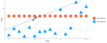
Figure 1: One sample convergent prices with Shannon Entropy=(0,4). The blue triangle represents the price of the more informed in different WTPs, and the orange rectangle represents the price of the less informed in different WTPs.

Figure 1 illustrates the Bait-and-Restrained-Exploit strategy in a representative sample with Shannon entropy $(0,4)$. The less informed AI offers a single price to all consumers, while the more informed AI can fully discriminate between consumers with different WTP. We can observe that for consumers whose WTP is 15, 18, 19, and 20, the more informed AI offers a strictly higher price. In other words, the more informed AI, although equipped with the full ability to discriminate prices, gives up the profits made in these segmented markets. Surrendering profits seems to be an irrational behavior, and given the strategy of the less informed AI, the more informed AI should adapt to lower its prices and thus capture profits in these markets. However, in an interactive context, this strategy component, called bait, entices the less informed AI to set a relatively high price at the cost of giving up profits in these markets. In turn, the more informed AI wins the remaining markets by setting a lower price. However, the price it offers is much lower than the minimum of consumers’ WTP and the price offered by the less informed AI. Again, leaving excess profit room seems irrational, and given the strategy of the less informed AI, the more informed AI should adapt to setting prices slightly lower than its opponent’s price or just exactly the same as consumers’ WTP (if its opponent’s price is well above consumers’ WTP). However, in a competitive environment, this strategy component, called restrained exploit, can exclude the less informed AI from downward deviations. If the AI with information disadvantage explores locally with lower prices, it not only loses profit margin in the markets where it already occupies the market share, but also fails to conquer more markets because its offer prices are still higher than its opponent’s prices. Therefore, the less informed AI is reinforced to maintain this high price level.

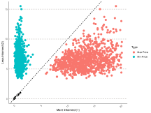
(a) Shannon Entropy=(0,4)

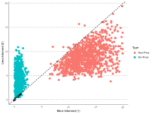
(b) Shannon Entropy=(0,3)

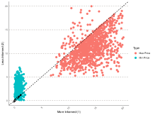
(c) Shannon Entropy=(0,2)

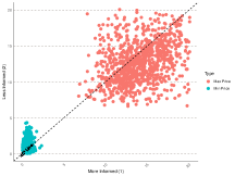
(d) Shannon Entropy=(0,1)

Figure 2: The maximum and minimum prices of firms. Each graph represents the two AIs’ prices with a pair of Shannon entropy. Each dot in figure represents a pair of convergent price in one simulation. The red dots represent the maximum prices set by two AIs, and the green dots represent the minimum prices.

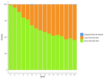
(a) Shannon Entropy=(0,4)

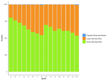
(b) Shannon Entropy=(0,3)

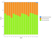
(c) Shannon Entropy=(0,2)

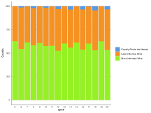
(d) Shannon Entropy=(0,1)

Figure 3: Market share of firms. Each graph depicts the market shares obtained by the more informed and the less informed firms under a pair of Shannon entropy values at different WTP levels. The green color represents the market share of the more informed firm, the yellow color represents the market share of the less informed firm, and blue indicates an equal split of the market between the two.

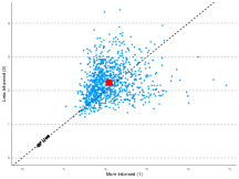
(a) Shannon Entropy=(0,4)

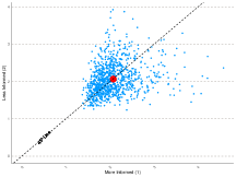
(b) Shannon Entropy=(0,3)

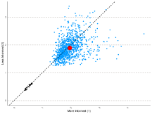
(c) Shannon Entropy=(0,2)

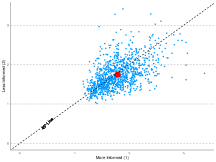
(d) Shannon Entropy=(0,1)

Figure 4: The profits of two firms with different Shannon entropy. The x-axis represents the profits of the more informed firms, while the y-axis represents the profits of the less informed firms. Each blue dot represents a pair of profits in one simulation, and red dots represent the average profits over 1000 simulations.

To demonstrate that the first part of Observation 1 is a general phenomenon, we plot the distribution of maximum and minimum prices offered by both AI agents in Figure 2.

The left figure 2(a) shows the scenario where one AI agent has full price discrimination capability, while the other AI agent can only offer a uniform price to consumers, i.e. with entropy level $(0,4)$. The mass of red dots, well below the 45-degree line, indicates that the information-advantaged AI consistently sets the maximum price strictly higher than that of the information-disadvantaged AI. Thus, the more informed AI is giving up profits in some markets. The mass of green dots, well above the 45 degree line with strictly positive gap, implies that the minimum prices set by the more informed AI are strictly lower than those set by the less informed AI. Therefore, the well-informed AI captures the remaining markets with restrained exploitation. The remaining three graphs document the pattern of maximum and minimum prices as information asymmetries decrease. The mass of red and green dots both moving towards the 45 degree line indicates that the gaps between the maximum prices of these two agents and between the minimum prices are both shrinking. This implicitly implies that the tendency to adopt the Bait-and-Restrained-Exploit strategy, a way to manipulate less informed AIs into colluding, is reduced as the information advantage of more informed AIs diminishes.

The Figure 3 illustrates the market division scheme for various degrees of information asymmetry. The left figure 3(a) shows the situation with the greatest information asymmetry, i.e. with an entropy level of $(0,4)$. The more informed AI dominates the market, which consists of consumers with low WTP. The AI with information advantage captures almost the whole market of consumers with WTP 5 and 6. As consumers’ WTP increases, this dominance in market shares weakens. In markets where consumers’ WTP exceeds 15, the more informed AI has only about 50 percent of the market share. In the remaining graphs of Figure 3, within the same partition of signals for the less informed AI, its market share of segmented markets increases as the value of the segmented markets increases. Thus, it shows that the AI with information advantage is more likely to forgo profits in high-value markets while exploiting profits in low-value markets. The rationale behind this phenomenon is that more informed AI must refrain from over-exploiting profits, i.e., there is a strictly positive gap between the consumer’s WTP and the price offered by more informed AI. Therefore, more informed AI is almost indifferent between high and low valued markets. Thus, its profit is primarily determined by the number of “markets” it can capture. If it gives up high-value signals/markets, it may only need to surrender a small number of markets to successfully trick the less informed AI into setting high prices.

Figure 4 illustrates the third part of Observation 1. We can see that when the Shannon entropy of the information structure for the less informed AI is $1$, $2$, and $3$, the profit pair is located around the 45 degree line, implying that their profits are roughly equal. This argument can be further verified since the average profit pair is almost on the 45 degree line. However, when the Shannon entropy of the information structure for the less informed AI is $4$, i.e., when the information asymmetry reaches its extreme, the less informed AI can actually achieve a strictly higher expected profit. This observation contradicts the conventional wisdom that data advantage translates into competitive advantage in the marketplace. One possible reason is that less informed AI, which can only offer a single price to all consumers, is more difficult to collude with because it has to give up low-value markets by raising its offered prices. In order to achieve collusion, the more informed AI must, on the one hand, give up more high-value markets and, on the other hand, lower its prices and thus limit its exploitation in low-value markets. Thus, competitive advantage is sacrificed in exchange for collusion.

Figure 5 illustrates the fourth part of the Observation 1, where we fix the Shannon entropy of Firm 1’s information structure at 0 and vary the Shannon entropy of Firm 2’s information structure from 0 to 4. As the informativeness of Firm 2’s information structure decreases, the CI increases.

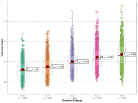
Figure 5: CIs with different Shannon entropy. The x-axis depicts the Shannon entropy under asymmetric information conditions. Each box represents the interquartile range, with the median indicated by the horizontal line and the mean by the red dot. The violin plot shows the distribution of the clustered sample set. Outliers, which are values outside 1.5 times the interquartile range above the upper quartile and below the lower quartile, have been excluded from the plot. The same below.

As the Shannon Entropy of the less informed AI increases, the average CI also increases from $0.26$ to $0.34$. Thus, information asymmetry leads to a higher degree of collusion. One possible explanation is that higher information asymmetry makes it easier for the more informed AI to manipulate the less informed AI and thus “teach” the less informed AI to collude.

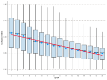
(a) Shannon Entropy=(0,4)

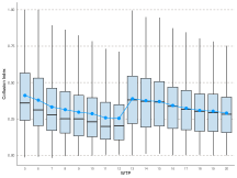
(b) Shannon Entropy=(0,3)

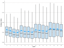
(c) Shannon Entropy=(0,2)

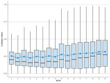
(d) Shannon Entropy=(0,1)

Figure 6: CIs of state (WTP) with different Shannon entropy. The x-axis represents WTP, and the y-axis represents the CI achieved at different WTP levels. Each box depicts the distribution of CIs under the corresponding Shannon entropy and WTP.

Finally, we draw the Figure 6 to show the last part of the Observation 1. In Figure 6, we plot a box plot of CI for each WTP under different pairs of Shannon entropies. We can see that within a single signal of the less informed AI, as WTP increases, the box goes lower and the regression line has a downward slope. Across the signals of the less informed AI, as WTP increases, the CI increases as WTP increases. In short, the trend of the CI shows a decrease within signals and an increase between signals.

Within a given signal scenario, the less informed firm can only offer a uniform pricing strategy. For those segments of WTP that are captured by the less informed firm, CI tends to decrease as WTP increases. Conversely, in segments where the more informed firm has a competitive advantage, although the price may increase as WTP increases, the increase is relatively modest and not proportional to the increase in WTP. This is due to the need for the price offered by the more informed firm to maintain a mark-up below the less informed firm’s uniform price in order to remain collusive. As a result, in these segments dominated by the more informed firm, CIs also show a downward trend.

In certain scenarios, such as when the less informed firm is completely unaware of the buyer’s WTP, it may strategically choose not to engage with buyers exhibiting low WTP in a monopolistic setting. This strategic choice implies that competition is inherently lower for segments with lower WTP than for those with higher WTP.

The observation that CI increases across signals serves as an extension of the Observation 4 noted in symmetric cases. The underlying rationale for this trend remains consistent in both scenarios. This pattern and its causes will be analyzed in detail in the next section.

5 Symmetric Information Structure

In this section, we consider the case where the two firms have a symmetric information structure. In reality, firms may buy data from the same third-party or even use the same third-party prediction. Sometimes competitors are forced to use the same consumer dataset. For example, when firms compete for a single advertising slot in Wechat moment, the Tencent increasingly relies on the first-price auction to allocate this slot. The Tencent will provide its own data to help companies evaluate the degree of match between the slot and their own products. Sometimes, the Tencent will close the interface to get access to firms’ own data. We find that strengthening price discrimination mitigates the collusion degree.

5.1 The Effect of Information Precision

We first examine how the degree of collusion varies with different levels of information precision, as indicated by Shannon entropy. Based on the evidence in Figure 9, we draw Observation 2.

Observation 2.

Collusion Index is increasing with respect to Shannon Entropy of the information structures.

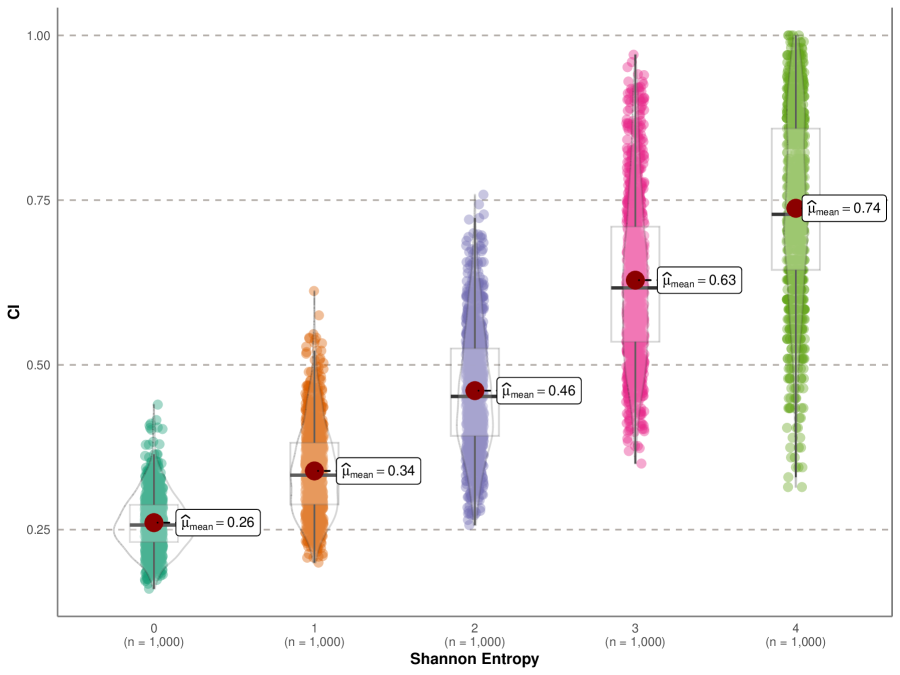
Figure 7: CIs of different Shannon entropy. Each group of graphs illustrates the distribution of the market-wide CI over 1000 simulations under the corresponding Shannon entropy.

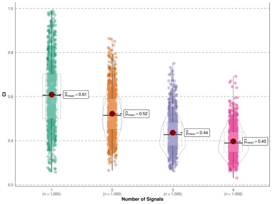
Figure 8: CIs of different number signals. For each of the 4 groups, each pair of AIs has 1, 2, 3 and 4 signals, respectively. The WTP is always 10, and all other settings are the same as the baseline.

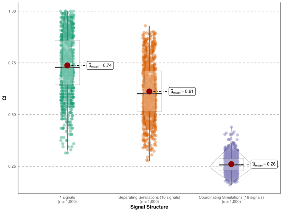
Figure 9: CIs of different signal structure. The first set shows single-signal outcome. In the second set, firms compete for one state. The last set shows coordinated competition across the most precise signals.

Figure 9 shows that as the Shannon entropy of the information structure increases, the average CI increases from $0.26$ to $0.74$. In addition, higher Shannon entropy also leads to higher variance in the CI. Intuitively, coarser information about consumers’ WTP introduces additional randomness into the system, and therefore the convergence outcome varies significantly if it is strictly above the Bertrand-Nash equilibrium.

This observation echoes with two classic arguments in industrial organization. First, in a static market game, more information increases competition and thus reduces firms’ profits, which is in the same spirit as the prisoner’s dilemma (see Thisse and Vives (1988); Shaffer and Zhang (1995)). However, this argument does not fit our setup perfectly, since it crucially relies on the assumptions of full rationality and a Bayesian decision maker. Moreover, Proposition 1 already implies that Bertrand competition is so fierce that any collusive outcome cannot be sustained by the equilibrium under any information structure. Second, in a repeated market game with more precise good signals, there should be stricter constraints on collusive behavior in the equilibrium path to preclude off-equilibrium deviations (see Miklós-Thal and Tucker (2019)). Again, this argument does NOT fit our framework, since Q-learning algorithms are not forward-looking, where they are programmed to make decisions based on what they have learned in the past. Moreover, the inactivation of one-step memory even precludes the possibility of making decisions depending on the opponent’s past behavior, a necessary assumption underlying the grim-trigger or carrot-stick strategy in repeated games.

This argument is also related to a recent paper Colliard et al. (2022), which shows that decreasing the uncertainty of the underlying state makes it easier for AI agents to learn competitive strategies and thus reduces the degree of collusion. However, the information structure in their paper is fixed, since AI agents always receive a single signal. Their framework cannot accommodate our setting where the information structure varies but the prior state distribution is fixed. To show that these three arguments cannot fully explain our results, we run the auxiliary experiments where the underlying state is certain and fixed at 10 (the expected WTP in the original experiments), and AI agents receive different numbers of payoff-irrelevant signals. The results are shown in Figure 9. Even in the absence of uncertainty, as the number of payoff-irrelevant signals increases from $1$ to $4$, the collusion index decreases from $0.60$ to $0.39$. This observation implies that, in addition to reducing uncertainty and enabling effective price discrimination, the information structure as a correlating device also plays a role in mitigating collusion. Before discussing how the correlating device works, we first compare the significance level of these two roles in mitigating collusion. Figure 9 compares the (average) collusion level under three scenarios: there are 16 uniformly distributed states with a single observed signal, there is only a single state, and there are 16 uniformly distributed states and 16 corresponding perfect-revealing signals. Compared to the first scenario, only the uncertainty is removed in the second scenario. Accordingly, the CI only decreases from 0.74 to 0.61. Compared to the second scenario, the third scenario includes a correlating device, but also removes uncertainty. The collusion index drops sharply from 0.61 to 0.26. Thus, in the original experiment, when the Shannon entropy is reduced from 4 to 0, the removal of uncertainty or the strengthening of price discrimination accounts for only 27.1 percent of the reduction in collusion, while the correlating device accounts for 72.9 percent of the reduction in collusion. Thus, the Observation 2 should be attributed more to the presence of the correlating device than to the removal of uncertainty or the reinforcement of price discrimination.

5.2 Potential Reasons

To address how the information structure affects the degree of collusion through the correlating device, we first answer how AI agents achieve collusive outcome under a single signal. Basically, similar to Colliard et al. (2022); Abada and Lambin (2023), we attribute the supra-competitive price to the failure to learn competitive prices. Suppose it starts with a price pair where player 2 wins the market. For any chosen price, as long as player 1 loses the market, his Q-value of that price decreases, forcing him to change his pricing strategy until he finds a lower price. Then it is player 2’s turn to search downward. We call this process sequential and alternating downward search. Ideally, as long as this process continues, the price level should converge to the Bertrand Nash equilibrium. However, this process can be interrupted because low prices cannot be maintained even if he wins the market and takes all the profit, because the Q-value of this low price is overestimated for some reason. If this process is interrupted, then both AI agents will search for other pricing strategies, and if by chance both agents choose the same relatively high pricing strategy at the same time, then they may converge at this supra-competitive price. For more details, see our accompanying note Xu et al. (2024), also attached in the Appendix D.

Then we move on to the multi-signal scenario. On the one hand, suppose that the AI agents are in fierce competition under certain signals $s_{a}$. The competition under these signals lowers their payoffs in the stage game and thus the Q-values of these signals. Under the remaining signals $s_{b}$, as the process of sequential and alternating downward search proceeds, suppose an AI agent $i$ has just found a lower price $p_{i}$ that can be sustained by the Q-value at signals $s_{b}$. Then it is the turn of the other AI agent $j$ to search downwards. During this process, if signals $s_{b}$ transition to signals $s_{a}$ with fierce competition, then the low Q-value at signal $s_{a}$ will significantly reduce the Q-value of price $p_{i}$ at signal $s_{b}$. This forces the AI agent $i$ to stop choosing $p_{i}$ at signal $s_{b}$ and to search for an appropriate price together with agent $j$, resulting in an interruption of the process of sequential and alternating downward search. Correspondingly, competition under certain signals increases the probability of interruption of the process of sequential and alternating downward search, thus increasing both the probability and the intensity of the collusive outcome under the remaining signals. And vice versa.

To support this reasoning, we further study the collusion degree among different signals by fixing the information structures. First, we study the empirical correlations between collusion levels among different signals. Pearson Correlation Coefficient is one of the classical correlation coefficients used to measure the strength and direction of the linear relationship between two continuous variables. The expression of Pearson Correlation Coefficient for CIs between signal $i$ and $j$ is

$$\rho_{ij}=\frac{\frac{1}{N}\sum_{t=1}^{N}(CI_{i}^{t}-\overline{CI}_{i})(CI_{j}^{t}-\overline{CI}_{j})}{\sqrt{\frac{1}{N}\sum_{t=1}^{N}(CI_{i}^{t}-\overline{CI}_{i})^{2}}\cdot\sqrt{\frac{1}{N}\sum_{t=1}^{N}(CI_{j}^{t}-\overline{CI}_{j})^{2}}}$$ (7)

where $N$ is the number of samples, $CI_{i}^{t}$ is the Collusion Index of the $t$ session under signal $i$, $\overline{CI_{i}}$ is the sample average of $\{CI_{i}^{t},t=1,2,\ldots,1000\}$. The correlation coefficients among collusion degree under various signals is plotted in Figure 10. Based on this figure, we then make Observation 3.

Observation 3.

Fixing information structure, collusion index among different signals are negatively correlated.

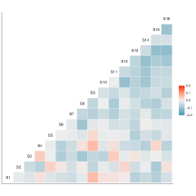
(a) Shannon Entropy=0

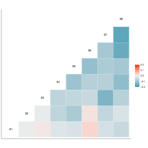
(b) Shannon Entropy=1

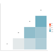
(c) Shannon Entropy=2

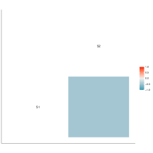
(d) Shannon Entropy=3

Figure 10: Correlation coefficient of CIs of different signals given information structure. The red block indicates a positive correlation in collusion level for the signals of the row and column corresponding to that block. And the blue block indicates a negative correlation.

Figure 10 shows the correlation coefficients of CIs between different signals at different levels of information precision. The graph is almost stacked with blue blocks, indicating negative correlations in collusion levels between signals. In other words, if both agents are in fierce competition on some signals, they are more likely to collude on the other signals. And vice versa.

It is argued that competition under certain signals facilitates collusive outcomes under the remaining signals. Then, under which signals are they more likely to compete or collude?

Observation 4.

The Collusion Index is higher in markets consisting of consumers with higher expected WTP.

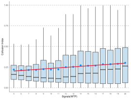
(a) Shannon Entropy=0

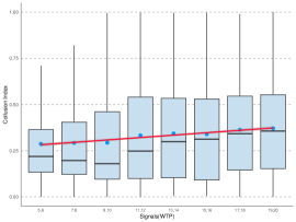
(b) Shannon Entropy=1

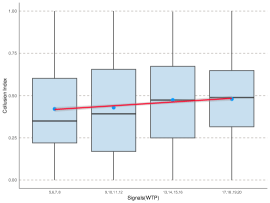
(c) Shannon Entropy=2

Figure 11: CIs of signals with different Shannon entropy. The blue dot represents the mean and the red line represents the regression line of CIs on signal groups. Outliers are omitted in the plot.

The Figure 11 plots the CI across signals for information structures with Shannon entropy $(0,0)$, $(1,1)$, and $(2,2)$, respectively. It shows that these AI agents seem to adapt to collude more in high-value markets, while competing fiercely in low-value markets. One possible explanation is that, given significant differences in WTP, a higher level of collusion in high-value markets generates a much higher level of Q-value compared to the Q-value in low-value markets. These higher levels of Q in high-value markets then stabilize the process of sequential and alternating downward search in low-value markets, facilitating the learning of competitive strategies. And vice versa. Therefore, it is more likely that AI agents will be more staggered in collusion outcomes. This observation is in stark contrast to the one in asymmetric information structure, where high-value markets in the same state partition end up with low collusion levels. This result again demonstrates that information structure also plays a key role in determining coordination among multi-agent reinforcement learning.

6 Welfare Analysis and Economic Implications

6.1 Welfare Analysis

AI’s use of data for price discrimination has profound implications for industry profits and consumer surplus. The critical questions revolve around the extent to which designers should provide data to AI to maximize the firm’s profit, and how to protect consumer surplus through data control measures.

We focus first on the impact of AI information precision on industry profits, as shown in Figure 12.

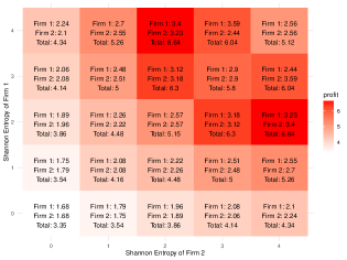
Figure 12: Industry Profits. Each block represents the average industry profits for each set of Shannon entropy in the respective group. Red indicates high industry profits, while white represents low industry profits.

Figure 12 shows that in symmetric scenarios, industry profits tend to decrease with increased data usage for discrimination, except in the extreme case of no data usage. Recall that in Observation 2, the CI is higher when the Shannon entropy is $(4,4)$ than when the Shannon entropy is $(3,3)$. However, the industry profits when the Shannon entropy is $(4,4)$ are lower than when the Shannon entropy is $(3,3)$. The main reason is that monopolistic profits are higher when the Shannon entropy is $(3,3)$ than when it is $(4,4)$. Moreover, one can see that from the Shannon entropy of $(4,4)$ to $(0,0)$, the industry profits first go up and then go down. This kind of inverted U-shaped trend is in line with certain theoretical results (e.g. Chen et al. (2001)). Moving from the Shannon entropy of $(4,4)$ to $(0,0)$, more precise information simultaneously increases transaction efficiency and reduces collusion. Once information precision exceeds a relatively modest benchmark of $1/8$ (the corresponding Shannon entropy is $(3,3)$), the adverse effects of reducing collusion begin to offset the gains in transaction efficiency, culminating in reduced profits.

In asymmetric situations, where the price discrimination ability of the more informed AI remains constant, the industry profits decrease as the less informed AI uses more data. Furthermore, we find that industry profits peak when the Shannon entropy pairs are either $(2,4)$ or $(4,2)$, and are lowest when both entities can perform first-order price discrimination. It is also apparent that blocks along the symmetry line appear more white than other nearby regions, indicating that the more symmetric information would tend to induce higher consumer surplus and lower industry profits.

For all situations, the numbers in Figure 12 illustrate the distribution of profits among firms by placing them in the context of a standard static game. The Nash equilibria of this game are at points $(2,4)$ or $(4,2)$. If firms choose their prediction precision in a manner similar to human competition, they will choose a precision level of $1/4$ (corresponding to a Shannon entropy of 2) or no prediction precision (Shannon entropy of 4) in the equilibria, even if they have the ability to fully differentiate between different consumers. However, if firms provide accurate consumer WTP information to the pricing algorithms, Q-learning cannot pretend not to know these accurate predictions, resulting in a market outcome where the Shannon entropy is $(0,0)$. We think the most likely reason is that Q-learning is incapable of learning such sophisticated strategies. We refer to the behavior of Q-learning always using the most accurate signals as the pricing algorithm’s over-usage of data.

If we look at consumer surplus and social welfare in Figure 13, we see that the effect of AI information accuracy is opposite to that of industry profit.

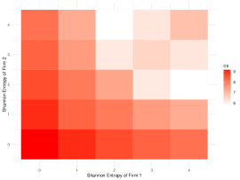
(a) Consumer Surplus

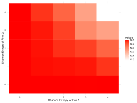
(b) Social Welfare

Figure 13: Consumer surplus and social welfare of different Shannon entropy. Each block represents the average consumer surplus (social welfare) for each set of Shannon entropy in the respective group. Red indicates high consumer surplus (social welfare), while white represents low consumer surplus (social welfare).

We observe that consumers generally benefit from firms’ data-driven discrimination, maximizing surplus when firms have the most accurate consumer information. This trend also holds for social welfare. For consumer surplus, blocks along the symmetry line appear more red than other nearby regions, indicating that more symmetric information would tend to induce higher consumer surplus and lower industry profits.

The reason for the effects of information precision is the same as we mentioned in the section on industry profits. On the one hand, as Shannon entropy decreases, firms gain more precise information about consumers, allowing flexible pricing strategies and increasing social welfare. On the other hand, lower entropy limits the ability of firms to collude effectively. Consumers benefit from both of the above channels, so that consumer surplus strictly increases as Shannon entropy decreases.

6.2 Economic Implication

The over-usage of data, which we propose in our analysis of industry profits, suggests that it may not always be beneficial for firms to incorporate extensive consumer data into their price discrimination systems. Therefore, for firms aiming to increase profits through big data and AI, this is one of the drawbacks of artificial intelligence, along with Calvano et al. (2023b); Bonelli (2022). Thus, firms aiming for high profits through algorithmic pricing should carefully choose the optimal information precision for algorithms, instead of providing the most precise data and letting the algorithm filter it.

It is important to note, however, that the reasoning behind our results is very different from human competition. In human competition, collecting more consumer data typically leads to higher profits, resembling a prisoner’s dilemma (Thisse and Vives 1988): regardless of opponents’ data holdings, acquiring more data is advantageous, even if it is detrimental to all parties if data collection increases across the board. However, in scenarios where AI replaces human participants, learning failures lead to collusive outcomes. In such situations, the accumulation of more data is always detrimental. Despite this, AI fails to recognize the detrimental effects and continues to engage in price discrimination, perpetuating the overuse of data.

Price discrimination can be exacerbated by competition, and algorithmic collusion is the second implication. Price discrimination involves setting different prices for different groups of consumers. According to Proposition 1, the Bayesian Nash equilibrium in human pricing involves both firms setting the lowest available action for each consumer. However, as shown in Observation 4, when firms use Q-learning to set prices, they tend to achieve higher collusion levels in markets with high WTP, resulting in generally higher prices for consumers with high WTP. As a result, algorithmic collusion could exacerbate price discrimination and raise fairness concerns.

The final implication underscores that allowing firms to exploit data is not necessarily detrimental to consumers, regardless of factors such as algorithmic recommendations that directly increase consumer utility. A primary concern regarding the use of data is that firms may use consumer data to maximize profits at the expense of consumer surplus. However, our results suggest that in scenarios involving data-driven price discrimination, firms’ use of data can increase consumer surplus and social welfare. Moreover, even if only a single AI is allowed to engage in data-driven price discrimination, collusion may be reduced because the AI must set exceptionally low prices at certain signals to manipulate competitors, thereby benefiting consumers.

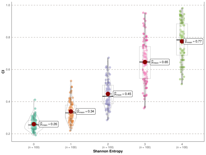
Figure 14: CIs of different Shannon entropy. Adjust the exploration rate of different information structure to make sure Q-learning can explore each cells of matrix 100 times, i.e., $\nu=100$.

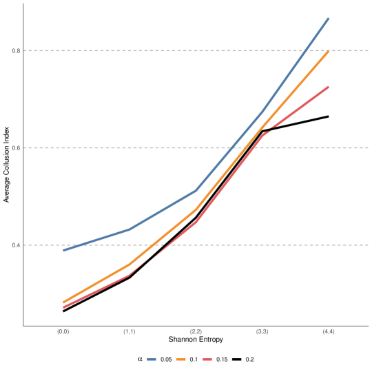
Figure 15: CIs of different Shannon entropy under different learning rate $\alpha$. Other parameters are set according to the baseline scenario.

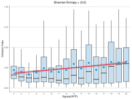
(a) Shannon Entropy=0

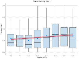
(b) Shannon Entropy=1

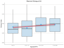
(c) Shannon Entropy=2

Figure 16: CIs of signals with different Shannon entropy. Adjust the exploration rate of different information structure to make sure Q-learning can explore each cells of matrix 100 times, i.e., $\nu=100$.

7 Robustness

In this preliminary vision, we focus on assessing the robustness of our baseline results to variations in specific parameters. In the future, we plan to conduct a more comprehensive evaluation of the stability of our results across different economic environments. All “experiments” in this section consists of 100 simulations.

Initially, we assumed a uniform value of $\beta$ in each information structure in our baseline simulations. This approach results in different frequencies of random exploration within each cell of the Q-matrix across different information structures. To address this, we aim to standardize the number of random exploration instances in each cell of the Q-matrix across all information structures to ensure uniformity. Specifically, we set $\nu=100$ as a constant number of random exploration instances for each cell. The corresponding $\beta$ values are then derived using the formula presented in Equation 6.

The results of our robustness evaluations are meticulously illustrated in Figure 15 and Figure 16. The CIs for each information structure are closely aligned with those observed in our baseline scenario. As a result, the Observation 2 remains valid. In addition, Figure 16 shows that, in general, the CI for each signal continues to show an upward trend along with the expected WTP.

Then, we explore the robustness of our results with respect to the learning rate, $\alpha$. Effective learning requires persistence, suggesting that $\alpha$ should be set to a relatively low value to ensure gradual integration of new information. In computer science, a commonly used value is 0.1, as highlighted in Calvano et al. (2020). To further validate the stability of our results, we examine the robustness of our findings across three additional values of $\alpha$, $0.05,0.1,0.2$. Figure 15 shows that regardless of the learning rate, the CI consistently increases with respect to the Shannon entropy of the information structures.

8 Concluding Remarks

We study Q-learning driven algorithmic collusion under different information structures in an uncertain environment, and identify two novel mechanisms that sustain collusion. Under asymmetric information structure, the AI with an information advantage employs a Bait-and-Restrained-Exploit strategy to lure the less informed AI into setting high prices. Under symmetric information, AIs compete in low-value markets to ensure the sustainability of collusion in high-value markets.

Furthermore, we observe that uncertainty, the absence of correlated signals, and information asymmetry intensify collusion, leading to a reduction in both consumer surplus and social welfare.

The implications of this article are threefold: First, the excessive use of data by AIs for price discrimination weakens collusion in competitive markets, highlighting an important drawback for firms to consider when adopting AI strategies. Second, competition and algorithmic collusion can exacerbate price discrimination, undermining fairness in the market. Furthermore, regardless of factors such as algorithmic recommendations that directly increase consumer utility, the results of this study suggest that firms using data do not necessarily harm consumers. Thus, a more nuanced perspective on companies that collect and use data is advisable.

For future research, three key areas merit attention. First, a more general theoretical exploration of algorithmic collusion is crucial to better understand its underlying mechanisms. Second, the study of market segmentation adds an interesting dimension to this work. Finally, providing empirical evidence on algorithmic collusion is essential to gain a deeper understanding of its dynamics.

Appendix A Proof of Proposition 1

It is straightforward that any player quoting $p^{N}=0$ is a BNE, and proving (3) is trivial.

(1) Let $P(p|\omega)$ denote the equilibrium transaction price distribution in state $\omega$ for $\omega\in\Omega$. We define $\overline{p}(\omega)$ as the maximum price in state $\omega$ with positive transaction probability, where $\overline{p}$ is the maximum of $\overline{p}(\omega)$ over all states in $\Omega$. The corresponding state is denoted by $\overline{\omega}$.

Suppose a player earns a positive profit, which implies the existence of a signal $s_{i}\in S_{i}$ for player $i$ with $\mu(s_{i}|\omega)>0$ and $p_{i}(s_{i})=\overline{p}$, with a positive probability of market participation under state $\overline{\omega}$. So there must also exist $s_{j}\in S_{j}$ for player $j$ with $\mu(s_{j}|\omega,s_{i})>0$ and $p_{j}(s_{j})\geq p_{i}(s_{i})$. Therefore, player $j$ optimally lowers the price quote on signal $s_{j}$ to $p_{i}(s_{i})-\eta$, where $\eta$ is small enough, since quoting the original price will at most share the market with others in any state. Consequently, in any equilibrium, $p(\omega)$ degenerates to a constant $0$ for all $\omega\in\Omega$.

(2) Without loss of generality, suppose that player $1$ offers $p_{1}>0$ under signal $s_{1}$. According to (1), there exists a signal $s_{2}$ such that $s_{1}$ and $s_{2}$ have a positive probability of occurring together, and player $2$ quotes $0$ under signal $s_{2}$. However, player $2$ has an incentive to bid higher on signal $s_{2}$ in order to make a positive profit.

Appendix B The Introduction of Q-Learning

B.1 Signal-Agent Q-Learning

Q-learning is a fundamental concept in reinforcement learning, a branch of machine learning where an agent learns to make decisions by interacting with an environment. At its core, Q-learning is a model-free, off-policy reinforcement learning algorithm used to find the optimal action-selection policy for a given finite Markov decision process.

In a stationary Markov decision process, in each period an agent observes a state variable $s\in S$ and then chooses an action $a\in A$. For any $s$ and $a$, the agent obtains a reward $\pi$, and the system moves to the next state $s^{\prime}$, according to a time-invariant (and possibly degenerate) probability distribution $P(s^{\prime},\pi|s,a)$. The goal of the agent is to find an optimal strategy $\Gamma^{\ast}:S\to A$ for choosing actions. A strategy $\Gamma(s)$ is optimal if in each state $s\in S$ it selects an action $a\in A$ that maximizes the agent’s cumulative payoff, which is the sum of its immediate payoff and its future payoffs.

Q-learning was proposed by Watkins (1989) to find an optimal strategy with no prior knowledge of the underlying model, i.e., the distribution $P(s^{\prime},\pi|s,a)$. The algorithm works by iteratively updating an action-value function $Q(s,a)$, which estimates the expected cumulative reward of taking action $a$ in state $s$. The key idea behind Q-learning is the Bellman optimal equation, which states that the optimal action-value function satisfies the equation:

$$Q(s,a)=\sum_{s^{\prime},\pi}P(s^{\prime},\pi|s,a)[\pi+\delta\max_{a^{\prime}}Q(s^{\prime},a^{\prime})],$$ (8)

where $0\leq\delta<1$ denotes the discount factor. If the values of the $Q$ function are known, an optimal strategy is given by

$$\Gamma^{*}(s)=\arg\max_{a\in A}Q(s,a).$$ (9)

Q-learning algorithm estimate the $Q$ values iteratively. Starting from an arbitrary initial matrix $\mathbf{Q}_{0}$, after choosing action $a$ in state $s$, the algorithm observes immediate payoff $\pi$ and next state $s^{\prime}$ and updates the estimated $Q$-values, denoted by $\hat{Q}$ using the update rule:

$$\hat{Q}(s,a)\leftarrow(1-\alpha)\hat{Q}(s,a)+\alpha[\pi+\delta\max_{a^{\prime}\in A}\hat{Q}(s^{\prime},a^{\prime})],$$ (10)

where $0<\alpha\leq 1$ is called the learning rate. Note that only for the cell $(s,a)$ visited, the corresponding $Q$-value $Q(s,a)$ is updated. It is proven in Watkins and Dayan (1992) that values $\hat{Q}(s,a)$ estimated will converge with probability $1$ to the optimal ones if each action is executed in each state an infinite number of times and $\alpha$ is decayed appropriately. In deterministic Markov decision process convergence of $\hat{Q}$ values can also be proven if a fixed value is used for $\alpha$ (Mitchell, 1997).

B.2 Exploration Policy

Exploration and exploitation are two fundamental concepts in reinforcement learning and decision-making processes. To have a chance to approximate the true $Q$ function starting from an arbitrary $\mathbf{Q}_{0}$, all actions must be tried in all states. Exploration allows the agent to discover the environment and learn about unknown states and actions. Exploitation, on the other hand, involves leveraging the information the agent already has to maximize immediate rewards. It entails choosing actions that are known to be rewarding based on past experiences or learned knowledge. Balancing exploration and exploitation is crucial for achieving optimal long-term performance in reinforcement learning tasks, as too much exploration may lead to inefficiency, while too much exploitation may cause the agent to miss out on potentially better actions or opportunities for learning. Strategies such as $\varepsilon$-greedy, Boltzmann exploration and upper confidence bound are commonly used in various reinforcement learning algorithms and decision-making contexts.

Appendix C Additional Figures

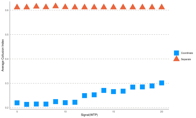
Figure 17: CIs of different signals with Shannon Entropy = (0,0). The blue rectangles represent the average CIs of the benchmark scenario, the orange triangles represent the average CIs when independently learning in different signals.

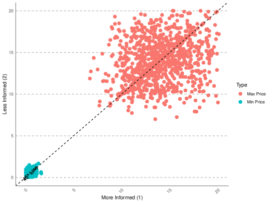
Figure 18: The maximum and minimum prices of firms when Shannon Entropy is (0,0).

Appendix D Note: Channel Underlying AI Collusion

In this note, we will explain why AIs cannot learn Nash equilibrium in most cases, even if there is no memory.

D.1 Q-Learning

Q-learning was proposed by Watkins (1989) to find an optimal strategy with no prior knowledge of the underlying model. Starting from an arbitrary initial matrix $\mathbf{Q}_{0}$, after choosing action $a$ in state $s$, the algorithm observes immediate payoff $r$ and next state $s^{\prime}$ and updates the one element of the Q-matrix corresponding to $(s,a)$ to be

$$(1-\alpha)\hat{Q}(s,a)+\alpha\left[r+\delta\max_{a^{\prime}}\hat{Q}(s^{\prime},a^{\prime})\right],$$ (11)

where $0<\alpha\leq 1$ is called the learning rate and $0\leq\delta<1$ denotes the discount factor.

To ensure that Q-learning sufficiently explores all states and actions, in this paper, we use the $\varepsilon$-greedy strategy. With probability $1-\varepsilon$, it chooses the action that is optimal according to the current Q-matrix and to randomize uniformly across all actions with probability $\varepsilon$. For a more detailed introduction to Q-learning, please see Appendix B.

In the special case that the environment is a Markov decision process that has only one state, this canonical Q-learning has a reduced form. Since the action taken in the current period does not affect the payoffs received in future periods, it follows that, in theory, maximizing the cumulative payoff is tantamount to maximizing the immediate payoff. Hence, the update rule reduces to

$$\hat{Q}(a)\leftarrow(1-\alpha)\hat{Q}(a)+\alpha r.$$ (12)

This signal-state Q-learning is a special case of the canonical Q-learning with the discount factor $\delta$ set to $0$. In the single-agent problems, if the environment has only one state, it is without loss of generality to use the reduced Q-learning algorithm. However, in multi-agent Q-learning framework, the discount factor $\delta$ is a crucial parameter that determines the game’s converging outcome, even if there is only one state. In the following context, “reduced Q-learning” refers to signal-state Q-learning, while “Q-learning” denotes the canonical Q-learning.

D.2 Experiment Design

We have constructed Q-learning algorithms and let them interact in a repeated Bertrand oligopoly setting. For each set of parameters, an “experiement” consists of 100 sessions. In each session, agent play against the same opponents until convergence as defined below.

Here we describe the economic environment in which the algorithms operate, discrete action space and other aspects of the numerical simulations.

D.2.1 Economic Environment

We take as our stage game the standard Bertrand pricing game. Consider firm $i\in N:=\{1,2,\ldots,n\}$ with marginal cost $c_{i}$. Firms sell homogeneous goods and compete by setting prices. The buyer’s reservation value for the good is denoted by $a$. In each period, a unit continuum of buyers enters the market. If there is no price lower than $a$, the buyers will leave the market without making a purchase. Otherwise, each buyer will randomly choose a firm with the lowest price to buy from. We denote the lowest price as $\underline{p}$. The set of firms with the lowest price (lower than $a$) is denoted by $\mathcal{I}:=\{i\mid p_{i}=\underline{p}\text{ and }p_{i}\leq a,\text{ for }i\in N\}$. We parameterize the model such that demand faced by firm $i$ is

$$q_{i}=\left\{\begin{aligned} &\frac{1}{\#\mathcal{I}}\quad&\text{if }i\in\mathcal{I},\\ &0\quad&\text{otherwise}.\end{aligned}\right.$$ (13)

The per-period reward accruing to firm $i$ is then $r_{i}=(p_{i}-c_{i})q_{i}$. In the symmetric setting, the unique Bertrand-Nash price $p^{N}$ is $c_{i}=c$ and the monopoly price $p^{M}$ is $a$ when the action space is continuous.

D.2.2 Action Space

Since Q-learning requires a finite action space, we need discretize the model. Similar to Calvano et al. (2020), we take the set $A$ of the feasible prices to be given by $m$ equally spaced points in the interval $\left[p^{N}+2\xi(p^{M}-p^{N}),p^{M}+\xi(p^{M}-p^{N}\right]$, where $\xi=1/m$. The rationale behind setting the lowest price as the Bertrand-Nash price plus twice the spacing is to ensure uniqueness of the Bertrand-Nash equilibrium in this discrete framework. Additionally, monopoly price is exactly in this set and we allow one price slightly higher than the monopoly price.

D.2.3 Other Settings

The following settings are the same as that in Calvano et al. (2020). Regarding the exploration mode, we also use the $\varepsilon$-greedy model with a time-declining exploration rate. Specifically, we set $\varepsilon_{t}=e^{-\beta t}$, where $\beta>0$ is a parameter. As for the initial matrix $\mathbf{Q}_{0}$, our baseline choice is to set the Q-values at $t=0$ at the discounted payoff that would accrue to player $i$ if opponents randomized uniformly.

D.3 Baseline Outcomes

In the baseline simulation, the Q-learning algorithms are memoryless (see Calvano et al. (2020) for the setting of memory). We focus on a baseline economic environment that consists of symmetric duopoly ($n=2$) with $c_{i}=c=0$, $a=1$, $\delta=0.95$, $m=20$. In the baseline simulation setup, we fix $\alpha=0.95$. To establish reasonable values for $\beta$, it is useful to relate $\beta$ to the expected number of times a cell would be visited purely through random exploration over an infinite time horizon, denoted by $\nu$. In the single-state without memory case, we have:

$$\nu=\frac{1}{m\left(1-e^{-\beta}\right)}.$$ (14)

For our baseline scenario, we set $\beta=5\times 10^{-4}$, which corresponds to $\nu\approx 100$ when $m=20$.

For strategic games played by Q-learning algorithms there are no general convergence results. To verify convergence, we use the following piratical criterion: convergence is deemed to be achieved if for each player either the action chosen in each state does not change for $100000$ consecutive periods which is a little different with the criterion in Calvano et al. (2020). We stop the algorithms if they do not converge after 1 billion periods.

To quantify the degree of collusion, we introduce a collusion index (CI), which is a normalized measure inspired by Calvano et al. (2020):

$$\operatorname{CI}:=\frac{\overline{r}-r^{N}}{r^{M}-r^{N}},$$ (15)

where $\overline{r}$ is the average total profit upon convergence, $r^{N}$ is the total profit in the Bertrand-Nash static equilibrium, and $r^{M}$ is the profit under monopoly. In our setting, $r^{N}$ is the lowest price in the discrete action space, ans $r^{M}$ is equal to buyer’s reservation value, $a$.

D.3.1 Collusion Index under Standard Q-Learning and Single-State Q-Learning

To compare the outcomes of the game played by standard Q agents and single-state Q agents, we focus on our baseline environment and explore the entire grid of the $20\times 21$ points by varying $\alpha$ in the range $[0.05,1]$ and $\beta$ in $[5\times 10^{-5},5\times 10^{-3}]$. Here, the lower and upper bounds of $\beta$ correspond to $\nu\approx 10$ and $\nu\approx 1000$ respectively.

Figure 19: Collusion Index for a Grid of Values of $\alpha$ and $\beta$ ($\delta=0.95$)

Figure 20: Collusion Index for a Grid of Values of $\alpha$ and $\beta$ ($\delta=0$)

Figure 20 and Figure 20 illustrate CI for grid values of $\alpha$ and $\beta$ in standard and single-state settings, respectively. It is evident that under standard Q with $\delta=0.95$, except for the region where $\alpha$ approaches $1$ and $\beta$ approaches $0$, the degree of collusion remains notably high. When $\alpha\leq 0.8$, even the lowest CI exceeds $0.59$. In contrast, under single-state Q, the CI is near $0$ across the grid, with the highest CI being $0.29$ occurring at $(\alpha,\beta)=(0.05,0.0018)$.

The first finding of the paper indicates that in a multi-agent game scenario, despite having only one state, standard Q agents and single-state Q agents exhibit notably distinct behaviors. Focusing solely on single-state Q agents within a one-state environment entails a loss of generality. Moreover, considering the uncertainty inherent in real economic environments or the prevalence and practicality of adding memory about past actions in algorithms, employing standard Q-learning to analyze single-state environments is more reasonable for a comprehensive depiction of reality.

Note that single-state Q-learning is merely a special case of standard Q-learning with $\delta=0$. The disparity in behavioral outcomes between the single-state Q agents and the standard Q agents in the game essentially stems from the variance in $\delta$. To delve deeper into the influence of the discount factor $\delta$ on collusive behavior among AI agents, Figure 22 demonstrates how CI fluctuates with variations in $\delta$ in the baseline environment. The trend indicates that with the increasing value of $\delta$, the degree of collusion tends to rise. This observation aligns with findings from Calvano et al. (2020), where Q-learning with memory was employed. When $\delta>0.7$, which is not overly stringent, CI surpasses $0.5$, indicating a significant level of collusion that cannot be ignored.

Figure 21: Collusion Index as a Function of the Discount Factor $\delta$ in the Baseline Setting

Figure 22: An Illustration of the Series of Q Values Throughout the Learning Process

D.4 Channel Underlying AI Collusion

To unveil the channels underlying AI collusion, we initially delve into the entire process of a single simulation. Figure 22 illustrates the series of Q-matrix values throughout the simulation. In the initial phase, the Q-values converge to nearly identical values, resulting in a Q-value “bubble”. Subsequently, agents sequentially and alternately downward search for lower prices to capture market share from their opponents. However, once their prices dip below a certain threshold, they rebound to the higher price and maintain it for an extended period. After numerous iterations of this process, in the third phase, they settle into a high collusion state as the exploration rate decays to zero.

To facilitate analysis, let us introduce some key concepts.

D.4.1 Sustainable Line and Stationary Line

We define a price as sustainable if, upon selection and monopolizing the entire market, its corresponding Q value will not decrease. Initially, we introduce the concept of a sustainable line, which represents the minimal price capable of sustaining the current chosen Q value. In our framework, the sustainable line is delineated by

$$p=(1-\delta)Q.$$ (16)

Should the selected price fall below the sustainable line, it fails to maintain its Q value. Even if it constitutes the best response to the opponent’s chosen price, the player will abandon this price in the subsequent period.

For a price profile $\mathbf{p}=(p_{1},p_{2})$, if it can sustain under Q-matrix $\mathbf{Q}$ indefinitely without exploration, we designate $\mathbf{p}$ as the stationary price profile under $\mathbf{Q}$. Notably, if $\mathbf{p}$ is a stationary price profile, then $p_{1}=p_{2}$. To simplify, we denote $p$ as a stationary price under $\mathbf{Q}$ if $\mathbf{p}=(p,p)$ represents the stationary price profile under $\mathbf{Q}$.

While a high price is sustainable, it may not persist as the stationary price. In the stationary price scenario, both agents choose the same price, resulting in each agent receiving half of the price as immediate profit. We introduce the stationary line as

$$p=2(1-\delta)Q.$$ (17)

If the price falls below the stationary line, it cannot remain as a stationary state under current Q-matrix. The stationary line is exactly twice the value of the sustainable line, allowing Q to search lower prices but preventing it from stabilizing at a low price.

D.4.2 Bubble

Due to the high exploration in the initial periods, the Q-values of each price converge to the same value, typically ranging from $6.5$ to $7.0$, regardless of the different initial values. This process injects a “bubble” into the Q-value, wherein it overestimates the discounted profit of lower prices. This bubble induces that prices lower than $0.32$ cannot be sustainable, and prices lower than $0.65$ cannot be stationary.

The crucial aspect of stabilizing at the lowest price lies in eliminating the bubble. However, accomplishing this debubbling process is highly challenging. Once they establish collusion at a high price, continuous exploration aimed at destabilizing the high price collusion will also inflate the bubble in the Q-value of lower prices. During the sequential and alternating downward search (as detailed in the next subsection), the bubble diminishes. However, when rebounding to a high price and stabilizing, efforts to debubble become futile.

D.4.3 Sequential and Alternating Downward Search

Figure 24, illustrating the descending phase within the second stage of Figure 22, depicts a mechanism leading towards the lowest value. This mechanism is commonly observed in 1000 simulations and is named sequential and alternating downward search. “Sequential” denotes the sequential decrease in price, while “alternating” signifies that agents lower their prices alternately.

Initially, starting from a high collusion point, after sufficient exploration (the last exploration being when agent $1$ [blue] explores to the lowest price, marked by a red background), agent $2$ (red) first learns to adjust its price downwards to maximize its profit. However, agent $1$ does not immediately respond due to the persistence of a high Q-value associated with the higher price. This delayed reaction leads to a rise in agent $2$’s Q-value corresponding to this new price. Subsequently, as agent $2$ begins to search for a more competitive price (i.e., a lower price), agent $1$ maintains its price at a constant level. This aspect can be viewed as a stationary learning process for agent $2$, enabling him to discover a lower price.

After the sequential and alternating downward search, agent $2$ first quotes a price below the sustainable line, indicating that the immediate payoff is insufficient to sustain its corresponding Q-value. Subsequently, agent $2$ abandons this price and explores other options. However, since agent $1$’s price is almost at the sustainable line, agent $2$ struggles to find a price that yields positive profit and is sustainable. As a result, agent $2$ occasionally revisits this price below the sustainable line. This situation hinders agent $1$ from maintaining their price, leading both agents to continually select prices in a chaotic manner.

D.4.4 Rebound

In this chaotic process, the Q-value gradually decreases, with the speed of decrease being slow and dependent on the learning rate $\alpha$. A higher $\alpha$ leads to a quicker decrease in the Q-value, reflecting a general decrease in the collusion index with an increase in $\alpha$. However, as the Q-value decreases, agents have a higher probability of sustaining at a high price, halting the Q-value decrease and transitioning to an increase.

The likelihood of both agents choosing the same high price is not low due to the relatively high Q-value associated with a high price, as it deviates from a collusion state. This higher Q-value increases the probability that agents will select a high price. Moreover, it is not necessary that they rebound to the same price simultaneously. If, at some point, they both opt for high prices, the agent with the relatively lower price will sustain, while the agent with the relatively higher price will sequentially lower his price. If he luckily finds that relatively lower price, they will establish a new collusion and stabilize there.

Furthermore, the stationary line may have a lower bound. If we approximate the chaotic process as random price selection, footnote 17 suggests that the lower bound of the stationary price is $0.67$, which is not insignificant. This convergence of the stationary line ensures that they will rebound to a high price again, albeit potentially different from the previous collusion.

Through the analysis above, we gain some insights into the underlying channel leading to collusion. The existence of a bubble is critical which results in two critical lines: the sustainable line and the stationary line. Even with agents learning to sequentially and alternately decrease their prices, once they surpass the sustainable line, their chosen price rebounds and often rebounds to higher prices. The stationary line, being sufficiently high, ensures that they ultimately rebound to a collusive state.

At the end, it is crucial to emphasize the dual effects of exploration. Firstly, exploration is pivotal in disrupting collusive states, leading to a phase of sequential and alternating downward search, thereby providing opportunities for Multi-agent Q-learning to converge to a Nash equilibrium. However, on the flip side, exploration is also the culprit behind bubble formation, preventing the stability of the minimum value and rebounding towards a collusive outcome. Moreover, a higher exploration rate accelerates the rate of bubble formation, making it more challenging to converge to a Nash equilibrium.

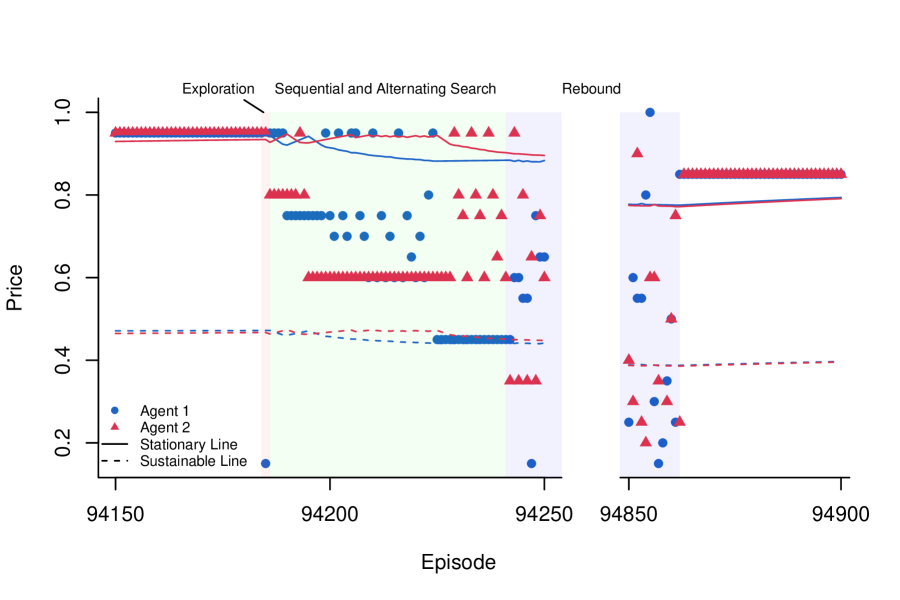
Figure 23: Visual Representation of Sequential and Alternating Downward Search and Rebound in the Baseline Setting

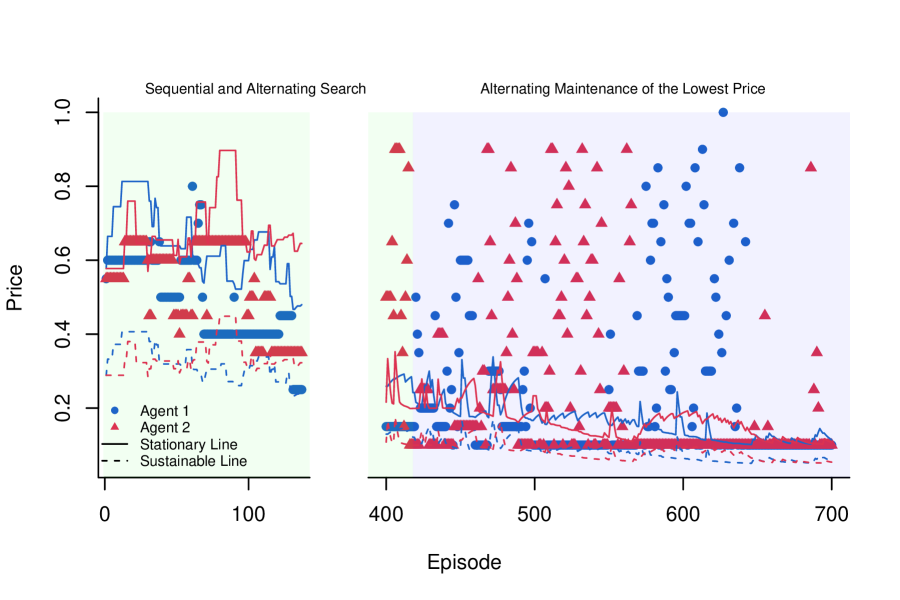
Figure 24: Visual Representation of Sequential and Alternating Downward Search and Alternating Maintenance of the Lowest Price ($\delta=0$, $\beta=0.005$)

D.5 Analysis of Parameters Effect

D.5.1 The Effect of the Discounted Factor

The emergence of bubbles sheds light on the effect of the discount factor $\delta$ on the degree of collusion. A higher $\delta$ leads to faster and more pronounced increases in the Q-values corresponding to lower prices, facilitating the formation of bubbles. In extreme cases, such as when $\delta=0$, the bubble phenomenon is absent.

If there were no bubble, after the initial extensive explorations, the Q-value for each price would be equal to the discounted profit in that price, assuming the opponent chooses prices randomly, equivalent to the initial Q-value we set. In a continuous action space $[0,1]$, the Q-value is easily calculated as $p(1-p)/(1-\delta)$, with the price yielding the maximum Q-value being $0.5$. In our discrete setting, the price with the maximum Q-value is $0.55$, setting the upper bound for collusion.

Figure 24 depicts the evolution of the best response price in a single simulation with $\delta=0$ and $\beta=0.005$. In the initial phase (green zone), agents engage in sequential and alternating downward search, as described earlier. Despite occasional rebounds due to high exploration rates, every chosen price must be sustainable due to the absence of the bubble, resulting in an overall downward search pattern. Around time $440$, agent $2$ (red) is the first to quote the lowest price of $0.1$. Subsequently, agent $1$ (blue) also adopts the lowest price. Once they reach the lowest price, the dynamic shifts, as rebounds become unlikely with no lower price to search for. However, because the lowest price is sustainable but unstable, transitioning to the stationary phase poses a challenge.

The subsequent phase (blue zone) describes this transition. Due to asymmetric Q-matrices, when both agents simultaneously choose the lowest price, one of them (agent $1$) is compelled to leave this price and search again, even though there are no more profitable alternatives available. Agent $2$ persists at the lowest price until agent $1$ recognizes that staying at the lowest price with only half the profit is beneficial. As a result, agent $2$ vacates the lowest price as agent $1$ returns and remains for an extended period. Subsequently, when agent $1$ leaves, agent $2$ returns, and vice versa, creating an alternating pattern of maintenance of the lowest price. The outcome is a decrease in Q-values to a level that ensures the lowest price becomes stationary.

As $\delta$ decreases, the lowest price becomes more likely to be sustainable. Consequently, the rebound process is replaced by the alternating maintenance of the lowest price. This shift ultimately leads from a collusive outcome to a competitive outcome.

D.5.2 Increasing the Lowest Action

The minimum action also significantly influences the degree of collusion. To investigate this, we varied the minimum value from 0.1 to 0.5 in increments of 0.01, resulting in 41 values, and conducted simulations in the baseline setting. Figure 26 depicts how the collusion index changes with the minimum action in the action space. Overall, it illustrates that as the minimum action increases, the collusion index decreases. Additionally, there exists a threshold $p^{\ast}$ around $0.3$. When the Bertrand-Nash price (i.e., the minimal price) $p^{N}\leq 0.26$, the collusion index hovers around $0.8$. Conversely, when $p^{N}\geq 0.33$, the collusion index drops to approximately $0$. In the interval $(0.26,0.33)$, the collusion index experiences a sharp decline.

Figure 25: Collusion Index and Price as a Function of the Lowest Action in the Action Space

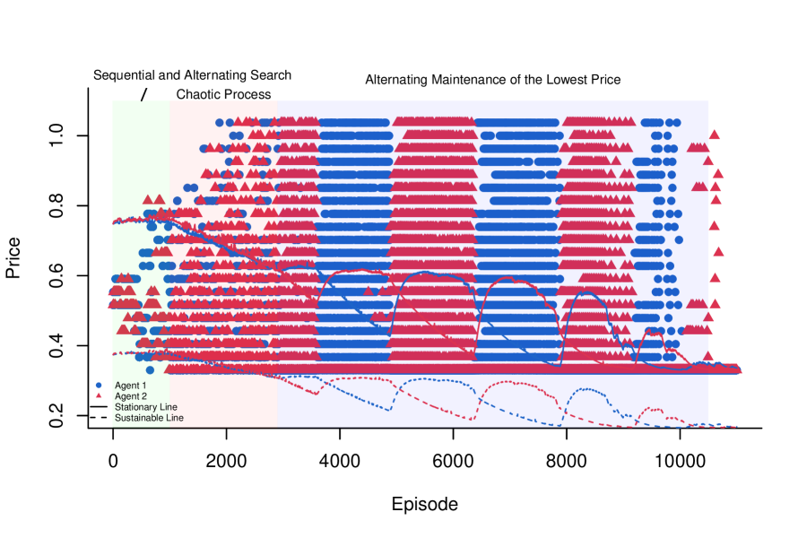
Figure 26: Visual Representation of Sequential and Alternating Downward Search and Alternating Maintenance of the Lowest Price (Minimal Action $p^{N}=0.33$)

The value $0.33$ is a familiar value that appears repeatedly in the preceding text. It represents the minimum price that the Q-value can sustain after random selection. When $0.33$ acts as the minimum value, the alternating maintenance of the lowest price occurs, leading to a competitive outcome. In Figure 26, we observe the evolution of the best response price in a single simulation where the minimal price is set to $0.33$. Initially, agents engage in sequential and alternating downward search. However, due to the presence of the bubble, $0.33$ proves unsustainable, resulting in a chaotic process and occasional rebounds to high prices. After several periods of random selection, $0.33$ becomes sustainable as the Q-values decrease during this chaotic process. Sequential and alternating downward searches persist during the chaotic process until the lowest price is identified, at which point the alternating maintenance of the lowest price becomes evident, particularly in the blue zone of the figure.

Conversely, when there are values falling below $0.33$, sequential and alternating downward search may result in unsustainable prices being selected, triggering rebounds and leading to a collusive outcome. Our analysis suggests that the occurrence of several values below $0.33$ (regardless of their exact number) impedes the alternating maintenance process and shifts towards rebounds, causing the collusion index to undergo a significant change around $0.3$, as we have observed.

The discount factor, $\delta$, is still a crucial parameter that influences the threshold value and the collusion index, especially when the minimum action is sufficiently low. The sustainability boundary is largely determined by the convergent Q-value following the initial high-frequency exploration phase. $\delta$ impacts not only the weight assigned to each cell of Q-matrix concerning the maximum Q-value but also the rate at which the bubble forms. When $\delta$ is sufficiently low, we cannot categorize the initial phase merely as a random selection process, and the convergent value of $6.7$ loses its effectiveness.

Figure 27: The Threshold as a Function of $\delta$

Figure 28: The Maximal Collusion Index as a Function of $\delta$

Figure 28 illustrates the variation of the threshold with $\delta$ ranging from $0.5$ to $0.99$, while Figure 28 illustrates the change in the maximal CI (CI under the minimal action) with $\delta$ in the same range. It is not surprising that both the threshold and maximal CI decrease with the decrease of $\delta$. The maximal CI exhibits an approximate linear relationship with $\delta$: when $\delta=0.99$, the corresponding maximal CI is $0.83$, while for $\delta=0.5$, it decreases to $0.25$, with a slope of approximately $1.2$. On the other hand, the threshold demonstrates an approximately logarithmic relationship with $\delta$. Specifically, when $\delta=0.99$, the threshold is $0.39$, whereas for $\delta<0.7$, it oscillates around $0.15$.

Figure 26 also depicts how the convergent price varies with changes in the minimum action. The minimum convergent price occurs at $p^{N}=0.33$, corresponding to $0.35$. While we introduce an exogenous markup over the competitive price, the additional markup induced by the dynamic learning process of Q-learning is disregarded. This finding bears economic implications: in the AI game, by allowing slight deterministic collusion (setting the minimum price they can choose higher than the competitive price), we can mitigate (and even almost eliminate) latent algorithmic collusion.

D.5.3 Increasing the Number of Actions

Since the action space is discrete, narrowing the price gap may impact collusion. Figure 31 illustrates the effect of the number of actions on collusion index when the minimum action is set to $0.2$ to $0.4$ with a $0.05$ spacing. The number of actions ranges from $10$ to $100$ with intervals of 10. To ensure sufficient exploration, we set different $\beta$ values corresponding to $\nu=100$. The results reveal a significant impact of the number of actions on points near the threshold $0.3$. As the number of actions increases, the collusion rate gradually decreases to around $0$ when the minimal price is near $0.3$. For example, if the minimal price is $0.3$, CI decreases from $0.77$ at $m=10$ to $0.02$ at $m=100$. However, the number of actions does not have a significant impact on the collusion index when the minimal price is near the two ends: $0.2$’s CI remains around $0.8$ and $0.4$ approaches $0$.

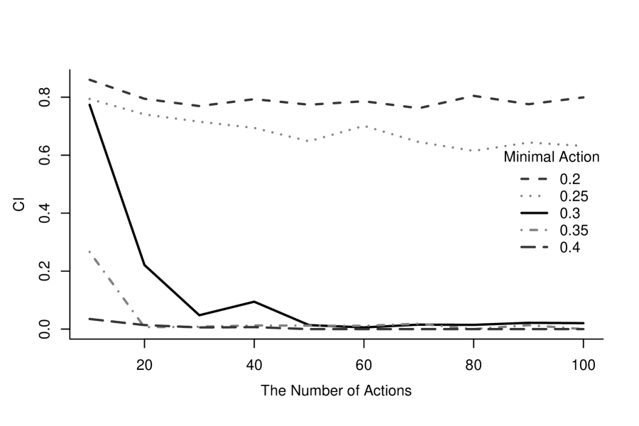
Figure 29: Collusion Index as a Function of the Size of the Action Space ($\nu=100$)

Figure 30: Collusion Index as a Function of the Lowest Action in the Action Space ($m=100$)

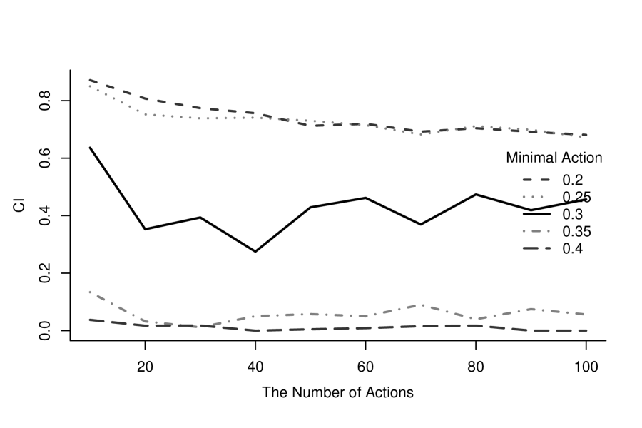
Figure 31: Collusion Index as a Function of the Size of the Action Space ($\beta=0.0005$)

Figure 31 illustrates CI as a function of the minimal action when the number of actions is $100$. The threshold in this case, with 100 actions, is $0.28$, which is lower than $0.3$. After initial exploration, the Q-value converges around $5.6$ when $m=100$, corresponding to a sustainable line at $p=0.28$. If the minimal price is larger than $0.28$, then alternating maintenance of the lowest price occurs; otherwise, rebounding is more likely, consistent with our previous analysis.

The last question pertains to why the convergent Q-value decreases with the number of actions. As the number of actions increases, exploration rates need to grow combinatorially rather than linearly to ensure thorough exploration of all price combinations. In the early periods, results can be seen as a combination of random and optimal selections. In our initial Q-value setting, optimal selections tend to favor lower prices, leading to a decrease in the convergent Q-value as the proportion of optimal selections increases with more actions.

Figure 31 also illustrates the effect of the number of actions but sets $\beta=0.0005$ as the baseline setting. We observe that the number of actions decreases collusion when the minimum action is lower but does not have a significant effect on the threshold. This implies the dual effect of exploration, as aforementioned: it disrupts collusion stability, thereby promoting competitiveness, and increases the speed of bubble generation, facilitating collusion outcomes. When the exploration rate remains constant as the number of actions increases, the inadequate learning, on one hand, fails to reach equilibrium results and thus does not significantly affect the threshold. On the other hand, premature convergence prevents bubbles from growing large enough to support high collusion, resulting in relatively mild collusion outcomes.

References

- Abada and Lambin (2023) Abada, I. and X. Lambin (2023, September). Artificial Intelligence: Can Seemingly Collusive Outcomes Be Avoided? Management Science 69(9), 5042–5065.
- Asker et al. (2022) Asker, J., C. Fershtman, and A. Pakes (2022). Artificial intelligence, algorithm design, and pricing. In AEA Papers and Proceedings, Volume 112, pp. 452–56.
- Asker et al. (2023) Asker, J., C. Fershtman, and A. Pakes (2023). The impact of artificial intelligence design on pricing. Journal of Economics & Management Strategy.
- Aumann (1987) Aumann, R. J. (1987). Correlated equilibrium as an expression of bayesian rationality. Econometrica, 1–18.
- Banchio and Mantegazza (2023) Banchio, M. and G. Mantegazza (2023). Adaptive algorithms and collusion via coupling. In Proceedings of the 24th ACM Conference on Economics and Computation, EC ’23, New York, NY, USA, pp. 208. Association for Computing Machinery.
- Banchio and Skrzypacz (2022) Banchio, M. and A. Skrzypacz (2022). Artificial intelligence and auction design. In Proceedings of the 23rd ACM Conference on Economics and Computation, EC ’22, New York, NY, USA, pp. 30–31. Association for Computing Machinery.
- Bergemann and Morris (2016) Bergemann, D. and S. Morris (2016). Bayes correlated equilibrium and the comparison of information structures in games. Theoretical Economics 11(2), 487–522.
- Bonelli (2022) Bonelli, M. (2022, November). Data-driven Investors.
- Calvano et al. (2020) Calvano, E., G. Calzolari, V. Denicolò, and S. Pastorello (2020, October). Artificial Intelligence, Algorithmic Pricing, and Collusion. American Economic Review 110(10), 3267–3297.
- Calvano et al. (2023a) Calvano, E., G. Calzolari, V. Denicolò, and S. Pastorello (2023a, September). Algorithmic collusion: Genuine or spurious? The 49th Annual Conference of the European Association for Research in Industrial Economics, Vienna, 2022 90, 102973.
- Calvano et al. (2023b) Calvano, E., G. Calzolari, V. Denicolò, and S. Pastorello (2023b). Artificial Intelligence, Algorithmic Recommendations and Competition. Algorithmic Recommendations and Competition (May 14, 2023).
- Calvano et al. (2021) Calvano, E., G. Calzolari, V. Denicoló, and S. Pastorello (2021, December). Algorithmic collusion with imperfect monitoring. International Journal of Industrial Organization 79, 102712.
- Chen et al. (2001) Chen, Y., C. Narasimhan, and Z. J. Zhang (2001). Individual marketing with imperfect targetability. Marketing Science 20(1), 23–41.
- Colliard et al. (2022) Colliard, J.-E., T. Foucault, and S. Lovo (2022). Algorithmic pricing and liquidity in securities markets. HEC Paris Research Paper.
- Dearden et al. (1998) Dearden, R., N. Friedman, and S. Russell (1998). Bayesian q-learning. Aaai/iaai 1998, 761–768.
- Dou et al. (2023) Dou, W. W., I. Goldstein, and Y. Ji (2023). Ai-powered trading, algorithmic collusion, and price efficiency. Available at SSRN 4452704.
- Epivent and Lambin (2022) Epivent, A. and X. Lambin (2022, August). On Algorithmic Collusion and Reward-Punishment Schemes.
- Forges (1993) Forges, F. (1993). Five legitimate definitions of correlated equilibrium in games with incomplete information. Theory and Decision 35, 277–310.
- Gautier et al. (2020) Gautier, A., A. Ittoo, and P. Van Cleynenbreugel (2020). Ai algorithms, price discrimination and collusion: A technological, economic and legal perspective. European Journal of Law and Economics 50(3), 405–435.
- Harsanyi (1968) Harsanyi, J. C. (1968). Games with incomplete information played by “bayesian” players part ii. bayesian equilibrium points. Management Science 14(5), 320–334.
- Johnson et al. (2023) Johnson, J. P., A. Rhodes, and M. Wildenbeest (2023). Platform design when sellers use pricing algorithms. Econometrica 91(5), 1841–1879.
- Klein (2021) Klein, T. (2021). Autonomous algorithmic collusion: Q-learning under sequential pricing. The RAND Journal of Economics 52(3), 538–558.
- Miklós-Thal and Tucker (2019) Miklós-Thal, J. and C. Tucker (2019). Collusion by algorithm: Does better demand prediction facilitate coordination between sellers? Management Science 65(4), 1552–1561.
- Mitchell (1997) Mitchell, T. M. (1997). Machine Learning.
- Shaffer and Zhang (1995) Shaffer, G. and Z. J. Zhang (1995). Competitive coupon targeting. Marketing Science 14(4), 395–416.
- Shannon (1948) Shannon, C. E. (1948). A mathematical theory of communication. The Bell System Technical Journal 27(3), 379–423.
- Thisse and Vives (1988) Thisse, J.-F. and X. Vives (1988). On the strategic choice of spatial price policy. American Economic Review 78(1), 122–137.
- Waltman and Kaymak (2007) Waltman, L. and U. Kaymak (2007). A theoretical analysis of cooperative behavior in multi-agent q-learning. In 2007 IEEE International Symposium on Approximate Dynamic Programming and Reinforcement Learning, pp. 84–91. IEEE.
- Waltman and Kaymak (2008) Waltman, L. and U. Kaymak (2008). Q-learning agents in a cournot oligopoly model. Journal of Economic Dynamics and Control 32(10), 3275–3293.
- Watkins and Dayan (1992) Watkins, C. J. and P. Dayan (1992). Q-Learning. Machine Learning 8, 279–292.
- Watkins (1989) Watkins, C. J. C. H. (1989). Learning from Delayed Rewards.
- Wu et al. (2023) Wu, J. X., Y. Wu, K.-Y. Chen, and L. Hua (2023). Building socially intelligent ai systems: Evidence from the trust game using artificial agents with deep learning. Management Science 69(12), 7236–7252.
- Xu et al. (2024) Xu, Z., M. Zhang, and W. Zhao (2024). Channel underlying ai collusion. Working Paper.