RADS : Restricted Anisotropic Diffusion Spectrum model for Axonal Health quantification in Multiple Sclerosis

Abstract

Axonal damage is the primary pathological correlate of long-term impairment in multiple sclerosis (MS). Our previous work using our method - diffusion basis spectrum imaging (DBSI) - demonstrated a strong, quantitative relationship between axial diffusivity and axonal damage. In the present work, we develop a variation and extension of DBSI which can be used to quantify the fraction of diseased and healthy axons in MS. In this method, we model the MRI signal with the axial diffusion (AD) spectrum for each fiber orientation, not just the mean axial diffusivity as is the case of basic DBSI. We use two component restricted anisotropic diffusion spectrum (RADS) to model the anisotropic component of the diffusion-weighted MRI signal. Diffusion coefficients and signal fractions are computed for the optimal model with the lowest Bayesian information criterion (BIC) score. This gives us the fractions of diseased and healthy axons based on the axial diffusivities of the diseased and healthy axons. We test our method using Monte-Carlo (MC) simulations with the MC simulation package developed as part of this work. First we test and validate our MC simulations for the basic RADS model. It accurately recovers the fiber and cell fractions simulated as well as the simulated diffusivities. For testing and validating RADS to quantify axonal loss, we simulate different fractions of diseased and healthy axons. Our method produces highly accurate quantification of diseased and healthy axons with Pearson’s correlation (predicted vs true proportion) of $r=0.99$ (p-value = 0.001); the one Sample t-test for proportion error gives the mean error of 2% (p-value = 0.034). Furthermore, the method finds the axial diffusivities of the diseased and healthy axons very accurately with mean error of 4% (p-value = 0.001). RADS modeling of the diffusion-weighted MRI signal has the potential to be used for Axonal Health quantification in Multiple Sclerosis.

1 Introduction

Multiple sclerosis (MS) is the most common progressive neurological disease of young adults, with a lifetime risk of one in 400 [7, 23, 5]. MS typically starts in young adults (mean age of onset, 20-30 years) and can lead to physical disability, cognitive impairment, and decreased quality of life [11]. It is an inflammatory-degenerative disease of the central nervous system (CNS) affecting approximately 2.3 million people worldwide, and affects nearly 1 million adults in the United States [25]. MS is characterized by inflammatory demyelination and irreversible axonal injury leading to permanent neurological disabilities [7, 23, 5, 11].

Axonal damage is the primary pathological correlate of long-term impairment in MS. The results in Ref. [[2]] demonstrate a strong, quantitative relationship between axial diffusivity and axonal damage. Diffusion tensor imaging (DTI) derived axial diffusivity and radial diffusivity have been previously used to detect and distinguish axon and myelin abnormalities [18, 8, 21, 22, 9, 12, 13]. In particular, decreased axial and increased radial diffusivity have been shown to reflect axonal and myelin injury respectively. Unfortunately, the DTI model does not address effects of inflammation-associated vasogenic oedema or increased cellularity. DTI is most accurate when applied to well-defined tightly packed white matter tracts without inflammation, as it is confounded by inflammation or crossing fibres [9]. The increased cellularity and vasogenic oedema associated with inflammation cannot be detected or separated from axon/myelin injury by DTI, limiting its clinical applications. To address these limitations of DTI based CNS imaging modalities, we developed diffusion basis spectrum imaging (DBSI) capable of characterizing water diffusion properties associated with axon/myelin injury and inflammation. DBSI thus provides a better imaging technique for early diagnosis of MS [10, 20, 15].

DBSI is an advanced multicompartment diffusion-based MRI technique that has the ability to isolate the signal contribution from different tissue compartments, thereby increasing the specificity for tissue subtypes and associated injuries. DBSI models myelinated and unmyelinated axons as anisotropic diffusion tensors, and cells and oedema/extracellular space as isotropic diffusion tensors to simultaneously quantify axonal injury, demyelination and inflammation in the CNS [26]. Diffusion basis spectrum imaging thus provides better insights into the MS pathology [10, 20, 15, 17, 4]. In the present work, we develop a variation and extension of DBSI which can be used to quantify the fraction of diseased and healthy axons based on the axial diffusivities of the axons in disease and in health.

2 Theory

In the case of anisotropic diffusion, the dependence of the normalized diffusion-weighted MRI signal $s$ on the diffusion tensor in a pulsed gradient spin echo experiment is given by the relation [14] :

$$s=\dfrac{s(b)}{s_{0}}=\exp{-b.\mathbb{r^{T}}\mathcal{D}\mathbb{r}},$$ (1)

where r is a unit column vector in the direction of the diffusion weighting gradient pulse, $\mathcal{D}$ is the diffusion tensor, $s_{0}$ is the signal without diffusion weighting, whereas $s(b)$ is the signal with diffusion weighting. The $b$ value is defined as :

$$b=\gamma^{2}G^{2}\delta^{2}\left(\Delta-\dfrac{\delta}{3}\right),$$

where $\gamma$ is the gyromagnetic ratio of hydrogen proton, $G$ and $\delta$ are the amplitude and duration of the diffusion gradient pulses, and $\Delta$ is the time between the leading edges of the gradient pulses.

Following Anderson’s work in [1], making the assumption that the diffusion tensor is axially symmetric, it can be diagonalized and written as

$$\mathbb{D}=\begin{pmatrix}\lambda_{\perp}&0&0\\ 0&\lambda_{\perp}&0\\ 0&0&\lambda_{\parallel}\\ \end{pmatrix}\,$$

in some coordinate system. Here $\lambda_{\perp}$ and $\lambda_{\parallel}$ are the radial and axial diffusivities of the axially symmetric tensor. Let $\alpha$ be the polar angle (the angle from the fiber axis) and $\psi$ be the azimuthal angle (relative to an arbitrary reference direction in the plane perpendicular to the fiber axis). Then diffusion in a particular direction, denoted by $D(\alpha$, $\psi)$, is given by

$$\begin{split}D(\alpha,\psi)=\\ \begin{bmatrix}\sin\alpha\cos\psi&\sin\alpha\sin\psi&\cos\alpha\\ \end{bmatrix}\begin{bmatrix}\lambda_{\perp}&0&0\\ 0&\lambda_{\perp}&0\\ 0&0&\lambda_{\parallel}\\ \end{bmatrix}\begin{bmatrix}\sin\alpha\cos\psi\\ \sin\alpha\sin\psi\\ \cos\alpha\end{bmatrix}\\ =\lambda_{\perp}+(\lambda_{\parallel}-\lambda_{\perp})\cos^{2}\alpha.\end{split}$$ (2)

In Diffusion basis spectrum imaging (DBSI) [26], the MRI signal is modeled as a linear combination of the isotropic and anistropic components. DBSI uses the simplification in Eq. 2 of axially symmetric tensor to model the anisotropic component of the signal. To account for muiltiple orientations of axons, the anisotropic component is modeled as a linear combination of signal contributions from different orientations. As a result, the signal in DBSI is modeled as :

$$s_{k}=\sum_{i=1}^{N_{aniso}}f_{i}e^{-b_{k}\lambda_{\perp i}}e^{-b_{k}(\lambda_{\parallel i}-\lambda_{\perp i})\cos^{2}\theta_{ik}}$$

$$+\int_{a}^{b}f(D)e^{-b_{k}D}d(D).$$ (3)

3 Methods

In the prsent work, we model the MRI signal with the axial diffusion spectrum for each fiber orientation, not just the mean axial ADC as in the case of basic DBSI. Furthermore, we assume fibers with the same radial diffusivity for each fiber orientation. Formally,

$$s_{k}=\sum_{i=1}^{N_{ori}}\sum_{h=1}^{N_{AD}}f_{ih}e^{-b_{k}\lambda_{\perp i}}e^{-b_{k}(\lambda_{\parallel ih}-\lambda_{\perp i})\cos^{2}\theta_{ik}}$$

$$+\int_{a}^{b}f(D)e^{-b_{k}D}d(D)$$ (4)

In Eq. 3, $s_{k}$ is the normalized diffusion-weighted signal corresponding to the $k$th diffusion gradient; $b_{k}$ is the b-value of the $k$th diffusion gradient ($k=1,2…N_{grads}$), where $N_{grads}$ is the number of gradient directions; $N_{ori}$ is the number of fiber orientations to be determined; $N_{AD}$ is the number of axial diffusion spectrum components to be determined; $\theta_{ik}$ is the unknown angle between the $k$th diffusion gradient and the $ith$ fiber direction; $\lambda_{\perp i}$ is the unknown radial diffusivity of the $i$-th anisotropic tensor corresponding to the $i$-th fiber orientation, and $\lambda_{\parallel ih}$ are the unknown axial diffusivities in the $h$-th component of the axial diffusion spectrum for the $i$-th fiber orientation; $f_{ih}$ is the unknown signal intensity fraction from the anisotropic tensor corresponding to the $i$-th fiber orientation and the $h$-th component of the axial diffusion spectrum; and $D$ is the diffusivity of the isotropic spectrum; and $a$ and $b$ are the low and high diffusivity limits for the isotropic diffusion spectrum $f(D)$.

For this work, we consider the case of a single fiber orientation, so that $N_{ori}=1$ and the corresponding radial diffusivity is $\lambda_{\perp}$. With these simplifications, the model in equation 3 reduces to -

$$s_{k}=\sum_{i=1}^{N_{AD}}f_{i}e^{-b_{k}\lambda_{\perp}}e^{-b_{k}(\lambda_{\parallel i}-\lambda_{\perp})\cos^{2}\theta_{ik}}$$

$$+\int_{a}^{b}f(D)e^{-b_{k}D}d(D),$$ (5)

where $f_{i}$ is the unknown signal intensity fraction from the anisotropic tensor corresponding to the $i$-th component of the axial diffusion spectrum; $\lambda_{\parallel i}$ are the unknown axial diffusivities in the axial diffusion spectrum.

3.1 Model Selection

For model selection as in Eq. 3, we solve a non-negative least squares problem. Choosing uniformly spaced $n_{1}$ points between $0$ and $3\times 10^{-3}mm^{2}/s$ for $\lambda_{\parallel}$ and $n_{2}$ discreet points between $0$ and $3\times 10^{-3}mm^{2}/s$ for $D$, and a fixed value for $\lambda_{\perp}$, we form the matrix $\mathcal{M}\in\mathbb{R}^{N\times{(n_{1}+n_{2})}}$ as follows.

$$\mathcal{M}=\begin{bmatrix}m_{1,1}&.&.&m_{1,n_{1}}&p_{1,1}&.&.&p_{1,(n_{1}+n_{2})}\\ m_{2,1}&.&.&m_{2,n_{1}}&p_{2,1}&.&.&.\\ .&.&.&.&.&.\\ &.&.&.&.&.\\ &.&.&.&.&.&.\\ m_{N,1}&.&.&m_{N,n_{1}}&p_{N,1}&.&.&p_{N,(n_{1}+n_{2})}\\ \end{bmatrix}$$ (6)

where

$$m_{k,i}=e^{-b_{k}\lambda_{\perp}}e^{-b_{k}(\lambda_{\parallel i}-\lambda_{\perp})\cos^{2}\theta_{ik}},$$ (7)

and

$$p_{k,i}=e^{-b_{k}D_{i}}.$$ (8)

With the above formulation, the model in Eq 3 can be rewritten in the discretized form as -

$$s_{k}=\sum_{i=1}^{n_{1}}f_{i}m_{ki}+\sum_{j=1}^{n_{2}}f_{j}p_{kj}.$$ (9)

In matrix form, the signal can be written as follows -

$$\begin{bmatrix}s_{1}\\ \dot{\textbullet}\\ \dot{\textbullet}\\ \dot{\textbullet}\\ s_{N}\end{bmatrix}=\begin{bmatrix}m_{1,1}&.&.&m_{1,n_{1}}&p_{1,1}&.&.&p_{1,(n_{1}+n_{2})}\\ m_{2,1}&.&.&m_{2,n_{1}}&p_{2,1}&.&.&.\\ .&.&.&.&.&.\\ &.&.&.&.&.\\ &.&.&.&.&.&.\\ m_{N,1}&.&.&m_{N,n_{1}}&p_{N,1}&.&.&p_{N,(n_{1}+n_{2})}\\ \end{bmatrix}\begin{bmatrix}f_{1}\\ \dot{\textbullet}\\ \dot{\textbullet}\\ \dot{\textbullet}\\ \dot{\textbullet}\\ \dot{\textbullet}\\ f_{(n_{1}+n_{2})}\end{bmatrix},$$ (10)

or, equivalently as

$$\mathbb{s=Mf}$$ (11)

The problem of model selection reduces to an optimization problem where our goal is to find the optimal values of $f_{i}$, $i=1,2,..(n_{1}+n_{2})$, with the constraints that $f_{i}$ take non-negative values. This is solved using non-negative least squares with $l2$ regularization as follows.

$$\min_{\mathbb{f}}\|\mathbb{s-Mf}\|+\beta\|\mathbb{f}\|_{2},\hskip 7.22743ptf_{i}>0\hskip 2.8903pt\forall i$$ (12)

For uniformly spaced values of $\lambda_{\perp}$ between $0$ and $0.4\times 10^{-3}mm^{2}/s$, we solve the minimization problem in Eq. 12, and pick the model with the least sum of squared residuals. This gives us the best fit model with the best fit radial diffusivity for the anisotropic component of the signal and the spectrum for the isotropic components.

3.2 Two component Restricted Anisotropic Diffusion Spectrum (RADS) model for Axonal Health

After solving the above minimization problem, we split the signal into anisotropic and isotropic components, and consider the anisotropic part of the signal $\mathbb{s^{an}}$ such that

$$s_{k}^{an}=s_{k}-\sum_{j=1}^{n_{2}}f_{j}p_{kj}.$$ (13)

While the isotropic components model the extra-axonal-extra-cellular and intra-cellular spins, the anisotropic component models the intra-axonal spins. For identifying the healthy and diseased axons, the anisotropic part of signal $s^{an}_{k}$ is modeled as a linear combination of average signal from each of the two components - healthy and diseased axons :

$$s_{k}^{an}=\underbrace{fe^{-b_{k}\lambda_{\perp}}e^{-b_{k}(\lambda_{\parallel 1}-\lambda_{\perp})\cos^{2}\theta_{1k}}}_{\text{unhealthy axons}}$$ (14)

$$+\underbrace{(1-f)e^{-b_{k}\lambda_{\perp}}e^{-b_{k}(\lambda_{\parallel 2}-\lambda_{\perp})\cos^{2}\theta_{2k}}}_{\text{healthy axons}}$$ (15)

where $f$ is the unknown signal intensity fraction from the anisotropic tensor corresponding to the unhealthy axons, and $(1-f)$ the signal intensity fraction from the anisotropic tensor corresponding to the healthy axons. With $\mathbb{M^{an}}$ defined as

$$\mathbb{M^{an}}=\begin{bmatrix}m_{1,1}&.&.&m_{1,n_{1}}\\ m_{2,1}&.&.&m_{2,n_{1}}\\ .&.&.&.\\ &.&.&.\\ &.&.&.\\ m_{N,1}&.&.&m_{N,n_{1}}\\ \end{bmatrix}=\begin{bmatrix}\mathbb{M^{an}_{1}}&\mathbb{M^{an}_{2}}&\ldots\mathbb{M^{an}_{n_{1}}}\end{bmatrix},$$ (16)

where the column vector $\mathbb{M^{an}_{n_{1}}}$ corresponds to the $\lambda_{\parallel}=2\times 10^{-3}mm^{2}/s$, assumed to be the axial diffusivity for the healthy axons. We solve the minimization problem again by using non-negative least squares for each value of $i$, $(1\leq i\leq n_{1}-1)$ :

$$\min_{f}\|\mathbb{s^{an}-M^{an}_{i}}f-\mathbb{M^{an}_{n_{1}}}(1-f)\|,\hskip 7.22743ptf>0.$$ (17)

This fitting process varied the $\lambda_{\parallel}$ values for the unhealthy compartment, keeping the $\lambda_{\parallel}$ for the healthy compartment fixed at $2\times 10^{-3}mm^{2}/s$; also the $\lambda_{\perp}$ was kept fixed at $0$. This minimization of the sum of squared residuals gives us $(n_{1}-1)$ models. We compare these models using Bayesian information criterion (BIC) [16], and the model with the lowest BIC score is chosen. The optimal model (having lowest BIC) gives us the fractions of diseased and healthy axons and the axial diffusivities of the diseased axons.

3.3 Monte-Carlo Simulations

Monte-Carlo (MC) simulations of spin diffusion as random walk are performed. The simulation geometry for the voxel includes uniformly spaced cylinders to model axons, and uniformly spaced spheres to model cells. The cylinders can penetrate the cells in the model. In a voxel as a cube with $100\mu m$ sides, we uniformly place cylinders modeling fibers with $1\mu m$ radius and $1\mu m$ inter-fiber distance ($3\mu m$ fiber center-to-center distance). For cells, we uniformly place spheres with $5.3\mu m$ radius. This is done such that the fibers make up $35\%$ of the voxel volume, and the cells make up $5\%$ of the voxel volume.

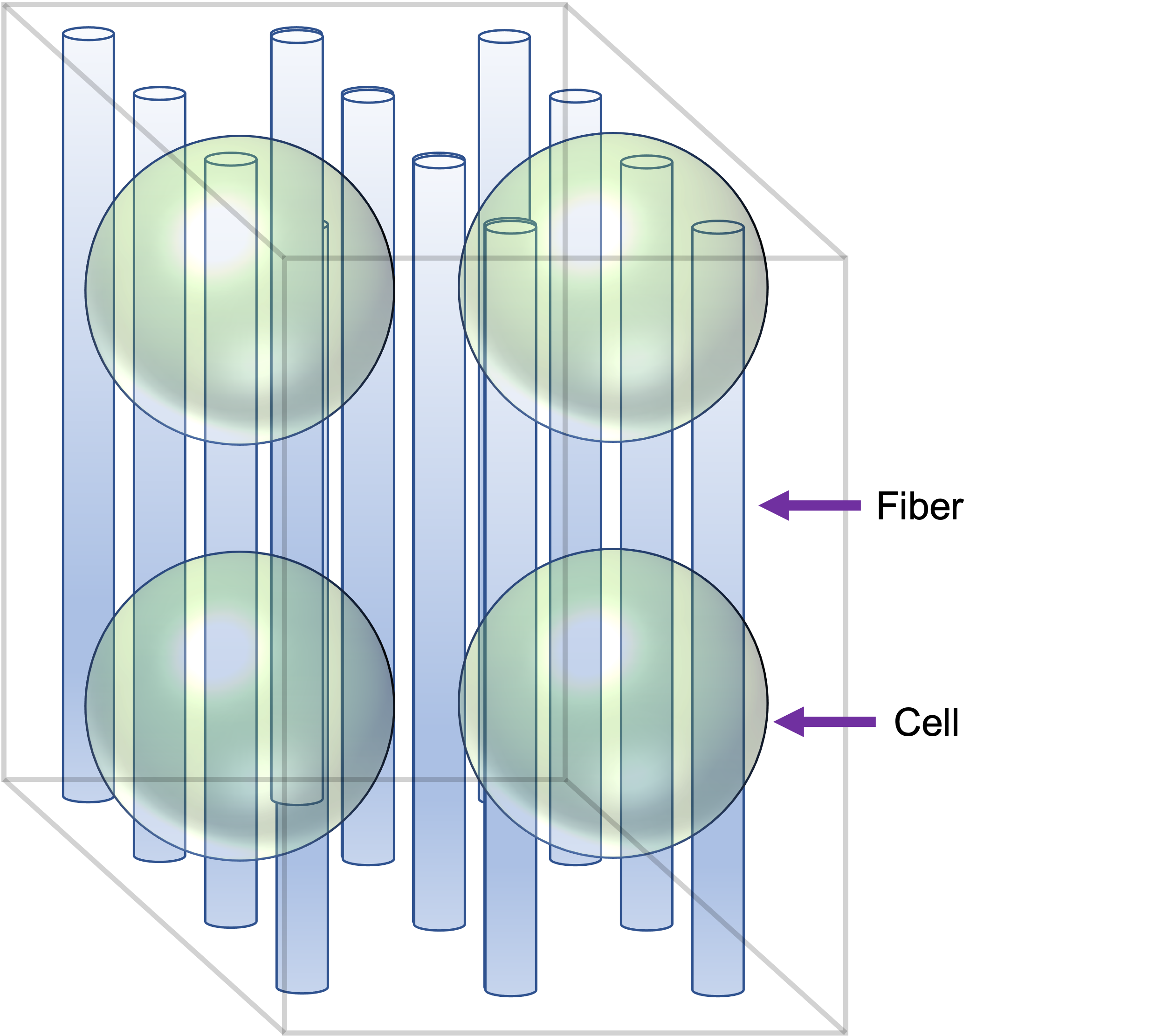
(a) Simulation Geometry

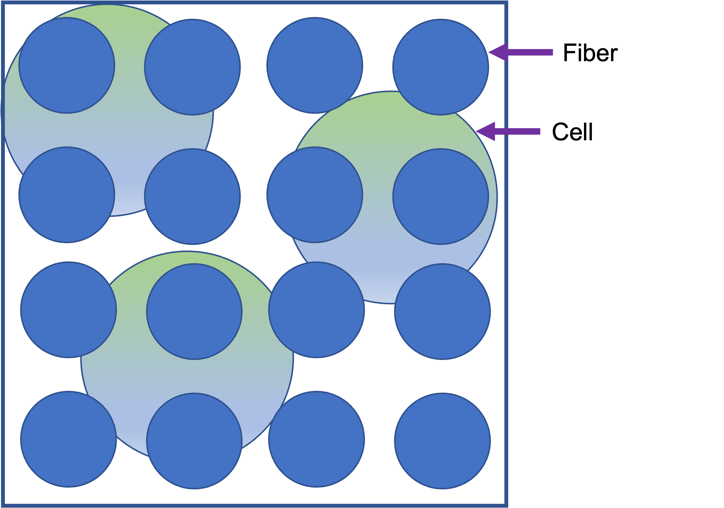
(b) Cross-sectional view

Figure 1: Monte-Carlo simulation geometry in a voxel with cylindrical axons, and spherical extra-axonal cells.

As the fibers pierce through the cells, the effective cellular volume was calculated as follows. Observe that the fiber volume enclosed in a sphere with radius $r$ centered at origin, with the fiber with radius $r_{1}$ centered at $(a,b,0)$ is the triple integral -

$$\int_{a-r_{1}}^{a+r_{1}}\int_{b-\sqrt{r_{1}-(x-a)^{2}}}^{b+\sqrt{r_{1}-(x-a)^{2}}}\int_{-\sqrt{r^{2}-(x^{2}+y^{2})}}^{\sqrt{r^{2}-(x^{2}+y^{2})}}dzdydx.$$ (18)

Subtracting the volume of all the fibers piercing through the sphere gives the net sphere volume. Observe that there will possibly be multiple configurations of fibers piercing the sphere which all need to be taken into account. With our voxel geometry, we get a cell fraction of $5\%$ with the spheres of $5.3\mu m$ radius.

As a result, we have three compartments in a voxel with different diffusion dynamics - Intra-axonal (IA), Intra-cellular-extra-axonal (ICEA), and extra-axonal-extra-cellular (EAEC). In the ICEA and EAEC compartments, the diffusivity is taken to be the free water diffusivity i.e. $3\times 10^{-3}mm^{2}/s$, whereas the diffusivity in the IA compatrment is assumed to be $2\times 10^{-3}mm^{2}/s$ for healthy axons.

For the random walk, we use $1,000,000$ spins distributed uniformly in the voxel. The number of spins is arrived at after detailed analysis of the number of spins required to stably and accurately produce the expected mean diffusivities as simulated. Recall that the squared displacement of the particles from their starting point over a time $\tau$ in free unrestricted diffusion (isotropic diffusion), averaged over all the sampled particles, is directly proportional to the observation time [6]. This is denoted as the Einstein Equation :

$$\left\langle r^{2}\right\rangle=6D\tau$$ (19)

where $\left\langle.\right\rangle$ accounts for the averaging operation, $r$ for the displacement and the scalar constant $D$, known as the self diffusion coefficient, measures the mobility of the particle ensemble. In the case of anisotropic diffusion, the analogous model is the diffusion tensor (DT) model proposed by Basser et al. [3]. Here the scalar diffusion coefficient D is replaced by a positive symmetric semi-definite matrix $\mathcal{D}$ representing diffusion, the diffusion tensor. Therefore, Einstein’s relation Eq. 19 is generalized, relating the covariance matrix of the net displacement vector $\textbf{R}\in\mathbb{R}^{3}$ and diffusion tensor $\mathcal{D}$ as

$$\mathcal{D}=\begin{pmatrix}\mathcal{D}_{xx}&\mathcal{D}_{xy}&\mathcal{D}_{xz}\\ \mathcal{D}_{xy}&\mathcal{D}_{yy}&\mathcal{D}_{yz}\\ \mathcal{D}_{xz}&\mathcal{D}_{yz}&\mathcal{D}_{zz}\\ \end{pmatrix}\,=\dfrac{1}{6\tau}\left\langle\textbf{R}\textbf{R}^{T}\right\rangle.$$

Diagonalization of diffusion tensor $\mathcal{D}$ gives the axial and radial diffusivities for the cylinderical IA compartment; for ICEA and EAEC compartments, the diagnolization gives the diffusivities in the $x,y,z$ directions. We use this diagnolization after using net displacements to find the number of spins that gives stable results in multiple simulation runs. We found that $1,000,000$ spins produce the required accuracy. With $1,000,000$, we get the expected mean diffusivities - radial and axial for anisotropic component, and isotropic diffusivities for free and cellular water - with acceptable variance for the purpose of our experiments.

Each spin takes a step in a random direction in the 3D space. This is achieved by using random 3D vector drawn from a normal 3D distribution, which is an effective and low cost method to get points uniformly spaced on a unit sphere, which gives uniformly distributed directions. The step size is taken to be $\sqrt{6Dt_{s}}$ where $t_{s}$ is the fixed time step, and $D$ is the diffusion coefficient. We use a time step of $5\mu s$ for our experiments. The detailed simulation parameters for the experiments are shown in Table 1.

Table 1: MC simulation parameters

Parameter	Simulated value
$\delta$	6 ms
$\Delta$	18 ms
Timestep	5 $\mu$s
Voxel side	100$\mu$m
Fibers volume	$35\%$
Cell volume	$5\%$
Fiber radius	$1-3\mu$m
Cell radius	$5-10\mu$m
No. of spins	$1,000,000$

When a spin encounters a barrier- either a fiber wall or a cell wall, the spin is reflected back from the barrier such that the spin remains in its compartment. The Figure 2 shows a few spin trajectories in the three different compartments. Diffusivity of water in EAEC and EAIC compartmets is taken to be $3\times 10^{-3}mm^{2}/s$. For fibers, we assume the diffusivity as $2\times 10^{-3}mm^{2}/s$ for the healthy axons.

(a) Spin trajectories in the three compartments

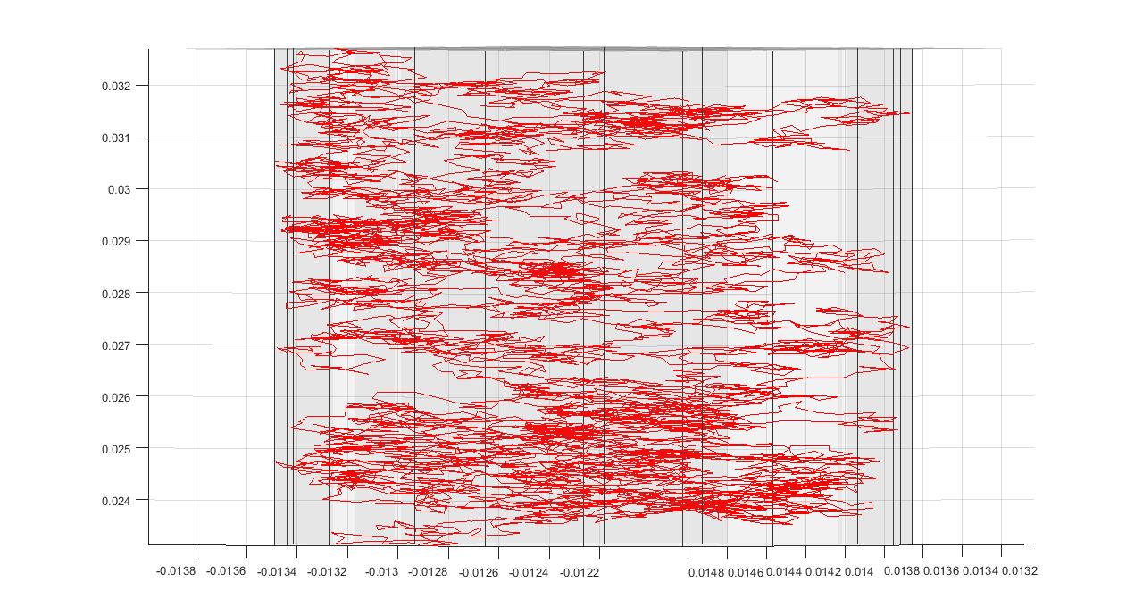
(b) Spin trajectory in the Fiber compartment

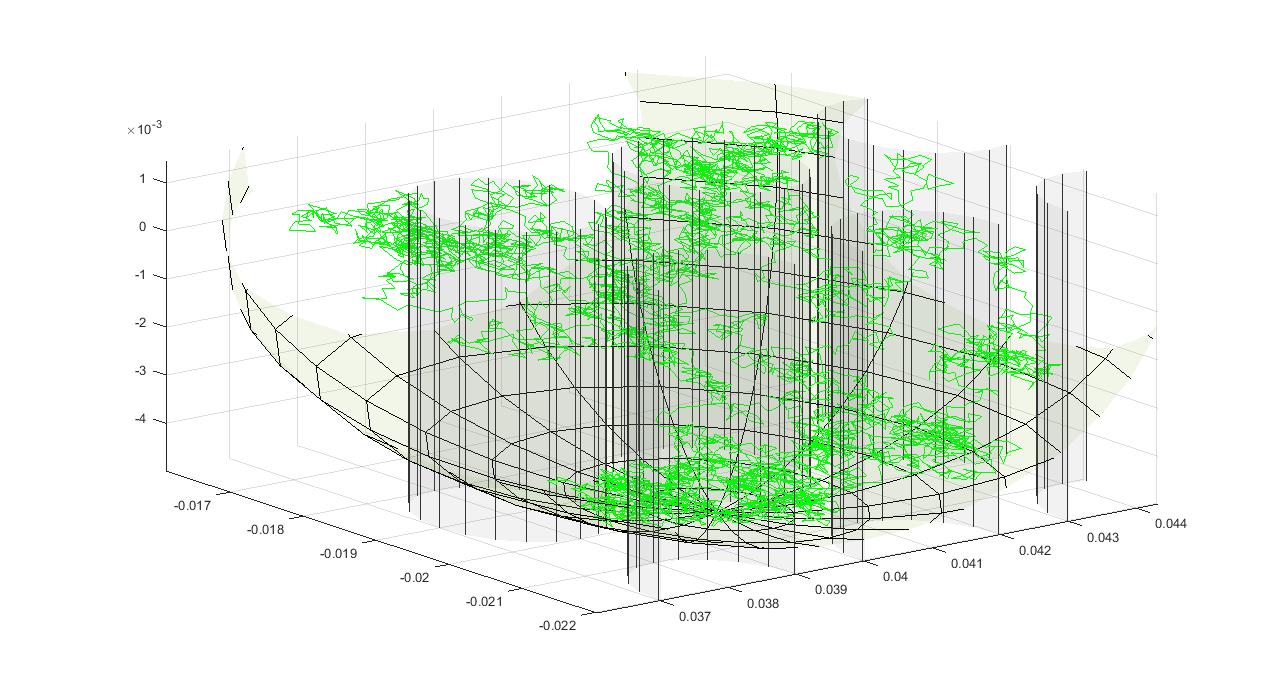
(c) Spin trajectory in the Cell compartment

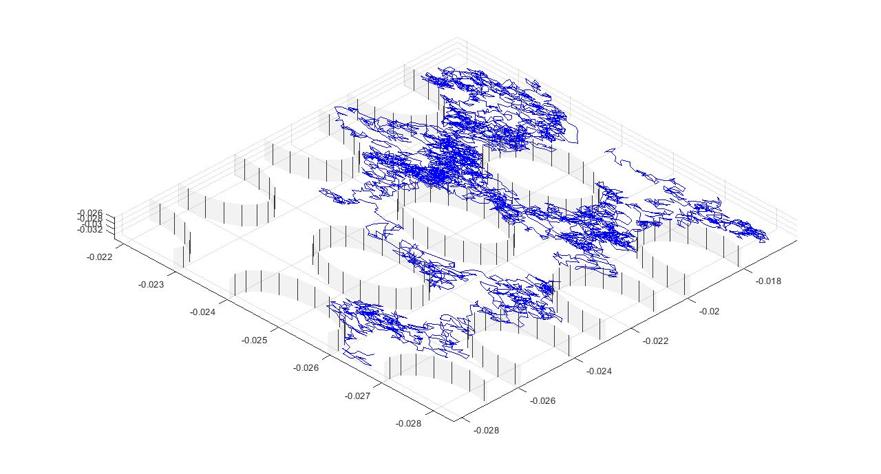
(d) Spin trajectory in the free compartment

Figure 2: Example Spin trajectories in MC simulations

3.4 PGSE Stejskal-Tanner sequence

The schematic of a Pulsed gradient spin-echo (PGSE) Stejskal-Tanner sequence [19, 24], used for simulations is shown in Figure 3.

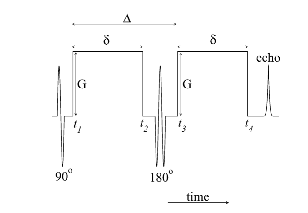
Figure 3: Pulsed gradient spin-echo (PGSE) Stejskal-Tanner sequence.

During the first half of the pulse sequence, a spin will accumulate a phase shift given by

$$\phi_{1}(\textbf{G},\delta)=\gamma\textbf{B}_{0}+\gamma\int_{t_{1}}^{t_{2}}\textbf{G}.\textbf{x}(t)dt,$$ (20)

where $\gamma$ is the proton gyromagnetic ratio (42 MHz/Tesla), G is the strength of the diffusion sensitizing gradient pulses, $\delta$ is the duration of the diffusion gradient pulses, and $\Delta=t_{3}-t_{1}$ is the time between diffusion gradient RF pulses. The phase shift experienced by each spin in the second half of the pulse sequence is given by

$$\phi_{2}(\textbf{G},\delta)=\gamma\textbf{B}_{0}+\gamma\int_{t_{3}}^{t_{4}}\textbf{G}.\textbf{x}(t)dt$$ (21)

The net phase shift experienced by a spin is the difference between the two phase shifts -

$$\phi(\textbf{G},\delta)=\phi_{1}(\textbf{G},\delta)-\phi_{2}(\textbf{G},\delta).$$ (22)

So, the net phase shift experienced by a spin is

$$\phi(\textbf{G},\delta)=\gamma\textbf{G}.\left(\int_{t_{1}}^{t_{2}}\textbf{x}(t)dt-\int_{t_{3}}^{t_{4}}\textbf{x}(t)dt\right)$$ (23)

For the system with the whole ensemble of spins, the signal is given by

$$S(t=TE)=S_{0}\int P(\phi,t)\mathrm{e}^{-i\phi}d\phi$$ (24)

The produced attenuated signal is then the result of the accumulated phase shift of the full assembly of spins at time TE, given by

$$S(t=TE)/{S_{0}}=\left\langle\mathrm{e}^{-i\int_{0}^{TE}\phi(t)dt}\right\rangle.$$ (25)

MC simulation uses finite number of spins $N_{s}$ so that the attenuated signal in Eq. 25 is approximated as

$$S(t=TE)/{S_{0}}=\dfrac{1}{N_{s}}\sum_{j=1}^{N_{s}}\mathrm{e}^{-i\sum_{1}^{N_{t}}\phi_{jk}(t)t_{s}},$$ (26)

where $N_{t}$ is the number of steps in the random walk, $\phi_{jk}$ is the phase shift of spin $j$ in step $k$, and $t_{s}$ is the time step.

We use fixed time step $t_{s}$, related to step length $l_{s}$ as

$$l_{s}=\sqrt{6Dt_{s}}$$ (27)

where $D$ is the diffusion coefficient. After the spin trajectories are simulated, the signal is computed using Eq. 26.

4 Results

Before simulating the axonal loss, we simulate and validate our model with simpler cases. These cases simulate a single average diffusivity for the random walk in all three compartments - the IA, the EAIC and the EAEC compartments. This is a useful first step to see what ADCs are observed for the isotropic components, and what axial and radial diffusivities are observed in the anisotropic part. We use the simple geometry of our voxel structure, to better control and observe the dynamics of the spins and how well our MC simulations and the model perform. To that end, as the first set of models, we consider only three directions diffusion weighting- $x,y,z$. Observe that in the $z$-direction, $\theta_{ik}=0$ and with a single average diffusivity in the IA compartment and , the the overall model in Eq. 3 reduces to :

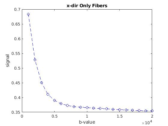
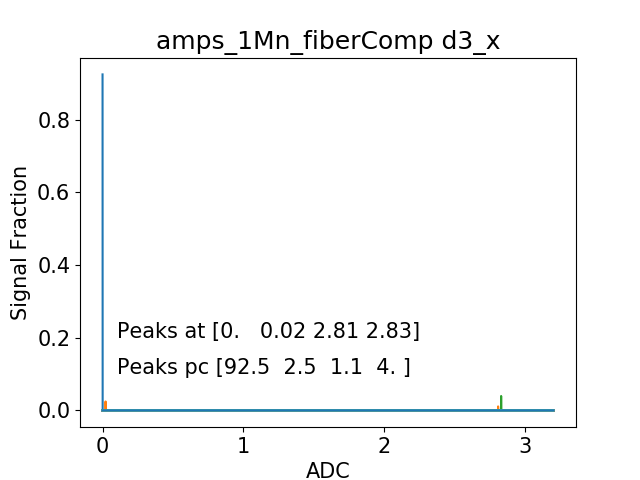
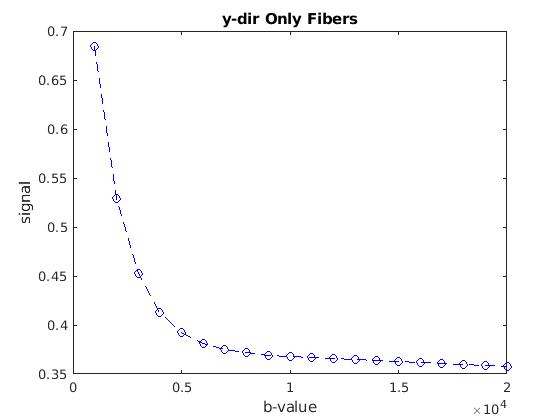
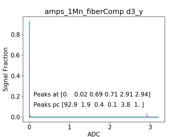
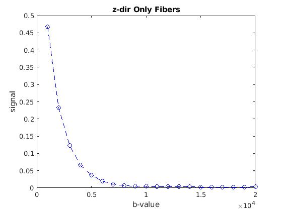
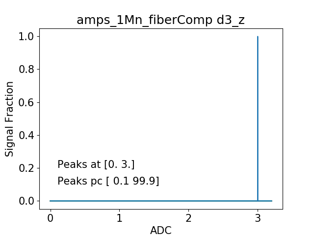
Figure 4: Fiber Compartment Signal and Signal Intensities.

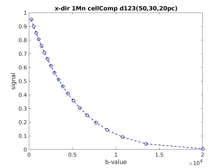
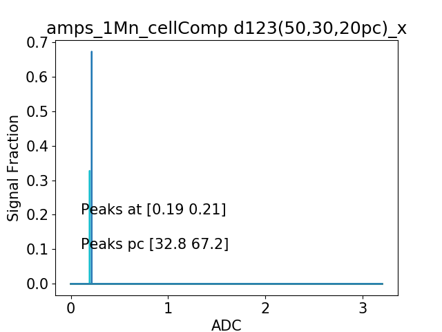
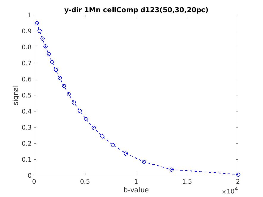
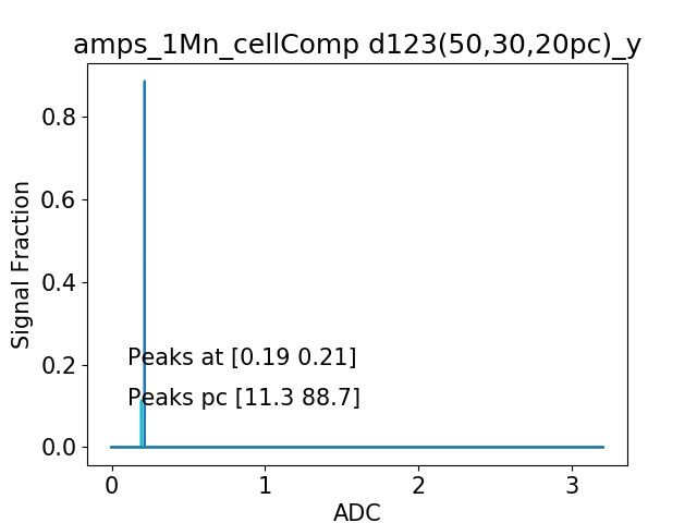
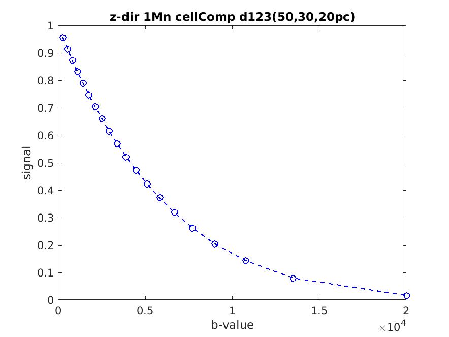
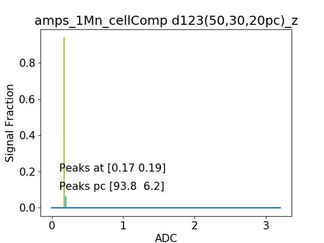
Figure 5: Cell Compartment Signal and Signal Intensities.

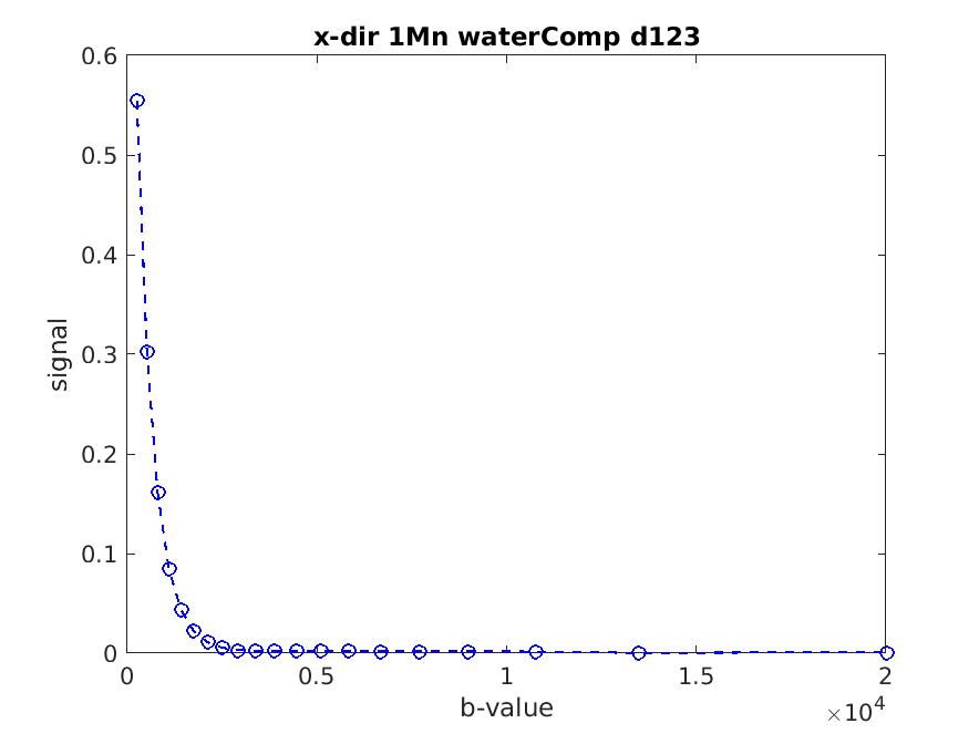
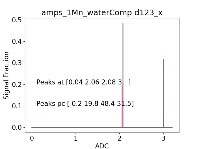
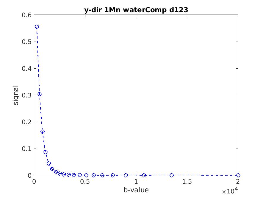
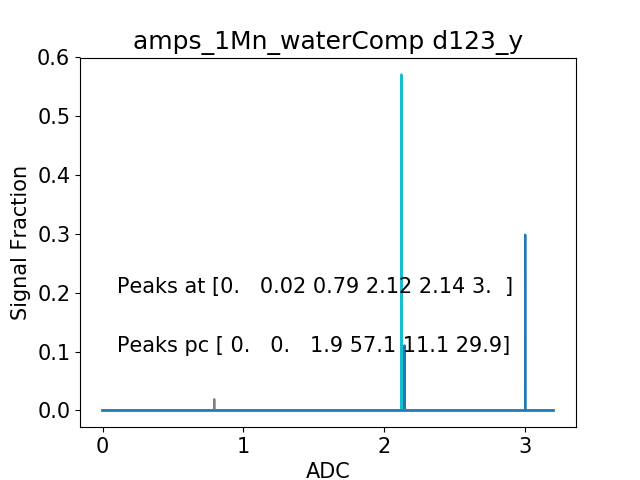
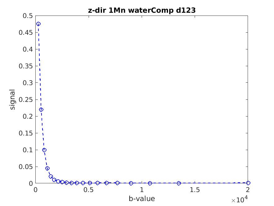
Figure 6: Free Water Compartment Signal and Signal Intensities.

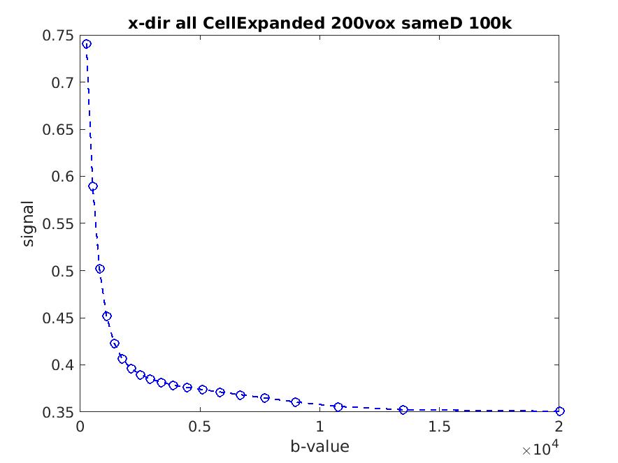
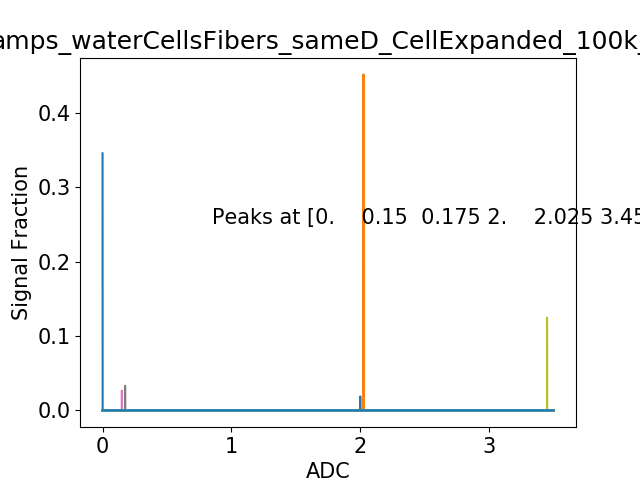
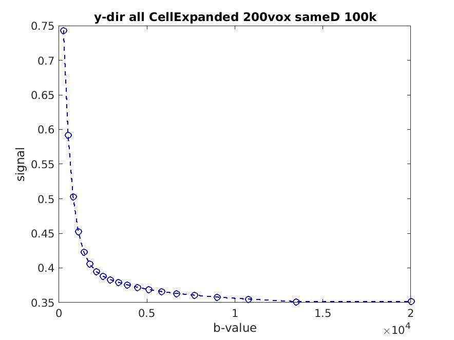
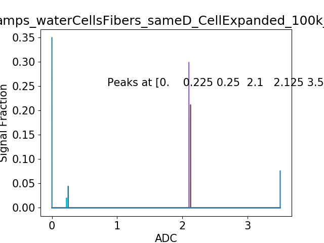
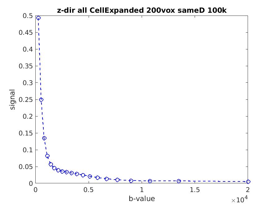
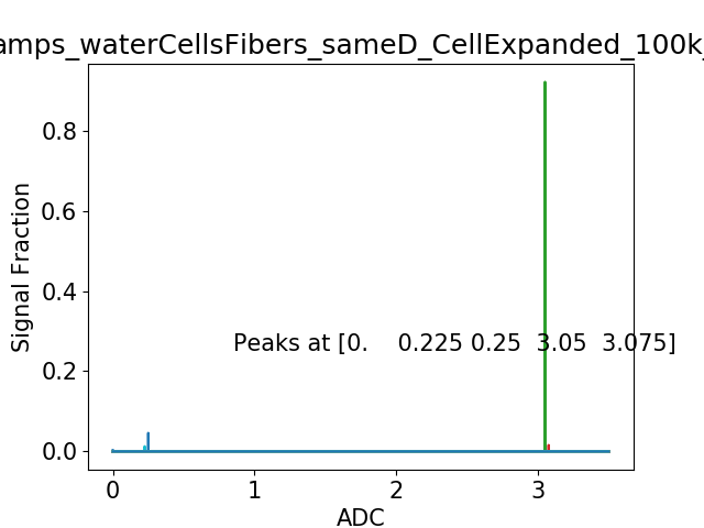
Figure 7: Full Structure Signal and Signal Intensities.

$$s_{k} =f_{1}e^{-b_{k}\lambda_{\perp}}e^{-b_{k}(\lambda_{\parallel i}-\lambda_{\perp})}+\sum_{j=2}^{n_{2}}f_{j}e^{-b_{k}D}$$ (28)

$$=f_{1}e^{-b_{k}(\lambda_{\parallel i})}+\sum_{j=2}^{n_{2}}f_{j}e^{-b_{k}D}$$ (29)

In the $x$ (and $y$)-direction, $\theta_{ik}=\pi/2$ and with a single average diffusivity in the IA compartment and , the the overall model in Eq. 3 reduces to :

$$s_{k} =f_{1}e^{-b_{k}\lambda_{\perp}}+\sum_{j=2}^{n_{2}}f_{j}e^{-b_{k}D}$$ (30)

Fitting the above two models for the three directions diffusion weighting- $x,y,z$- we get the signal as a combination of the exponential decay curves for each of the directions as shown in the figures below. Also shown are the corresponding signal intensities $f_{i}$ corresponding to each of the ADCs. Here, we simulate the following cases to validate our MC simulations and the model. The three compartments - the Fiber compartment, the cell compartment, and the Free water compartment - in the voxel are first simulated separately, and the model is validated. Then the full structure voxel is simulated and validated. The results are shown in Figures 4, 5, 6 and 7.

4.1 Key observations from $x,y,z$-directions diffusion weighted MC simulations

Based on the the basic MC simulations with for the three directions diffusion weighting- $x,y,z$, we discover that the best fit radial diffusivity $\lambda_{\perp}$ comes out to be $0$. Observe that in Figure 4, the signal decay in the $x$(and $y$)-direction is asymptotic to the signal intensity = 0.35, which is exactly the simulated fiber fraction. The corresponding ADC is made up primarily of $0$ (approx. $95\%$, if we include nearby ADC of $0.2\times 10^{-3}mm^{2}/s$); the remaining small fractions of higher ADCs can be explained by the model and simulation errors. As expected, for the cell compartment, the results shown in 5 are almost identical, with the small variability attributable to the sampling variability of the random walks.The average ADC in all the three directions is approximately $0.2\times 10^{-3}mm^{2}/s)$. For the water compartment, we get an average ADC of $2.33\times 10^{-3}mm^{2}/s)$ in the $x$(and $y$)-directions; and it is almost $3\times 10^{-3}mm^{2}/s)$ in the $z$-direction. A different and higher ADC in free water in the $z$-direction is an important insight into the diffusion dynamics in the voxel. This clearly tells us that there is some anisotropy present in the EAEC compartment in addition to the anisotropy of the fiber compartment. This is also confirmed by the Signal decay curves and corresponding ADC spectrum in the full structure as shown in Figure 7.

Having validated the baisc MC simulations and model, we simulate the axonal loss as follows. In the IA compartment, we simulate four cases where the fraction of axons with healthy axial diffusivity $\lambda_{\parallel}$, assumed to be $2\times 10^{-}3mm^{2}/s$, is reduced progressively from $100\%$ to $30\%$. The unhealthy axons are assumed to have $\lambda_{\parallel}$ as $1\times 10^{-}3mm^{2}/s$. The rest of the simulation parameters are the same as shown in table 1.

As detailed in the sections above, we first model the signal as in Eq. 9 and solved using the $l-2$ minimization problem as in Eq. 12. This is done with different values of radial diffusivity $\lambda_{\perp}$ between $0$ and $0.4\times 10^{-3}mm^{2}/s$, and finally the model with the least square residuals is selected. This first step in the DBSI-ADS method splits the signal into anisotropic and isotropic components. This model also gives us useful metrics - fiber fraction, cell fraction, best fit radial diffusivity $\lambda_{\perp}$. We run $10$ simulations with $1,000,000$ spins each. The results show a highly accurate recovery of the fiber and cell fractions.

While the ground truth fiber fraction is $35\%$, our model finds the fiber fraction very accurately. The One Sample t-test for fiber fraction gives the the fiber fraction as $34.83$, with 95 percent confidence interval: (34.10, 35.5) (P-value $<<0.0001$). Similarly for the cells, while the ground truth cell fraction is $35\%$, our model finds the cell fraction very accurately too. The One Sample t-test for fiber fraction gives the the fiber fraction as $5.37$, with 95 percent confidence interval: (4.98, 5.75) (P-value $<<0.0001$). The best fit radial diffusivity $\lambda_{\perp}$ comes out to be $0$, which also agrees with the results in the previous section.

In the second step, the anisotropic component of the signal is isolated. From this anisotropic part of the signal we have to deduct a small percentage of signal at the higher end of the anisotropic ADC spectrum which is from the anisotropy from the EAEC compartment. After extensive simulations and validations, we arrive at $4\%$ as the fraction that we deduct. The anisotropic component recovers the fiber and cell fractions very accurately, but axial diffusivity spectrum has a percentage of signal around ADC of $3\times 10^{-3}mm^{2}/s$, when the axial diffusivity simulated is $2\times 10^{-3}mm^{2}/s$ or less. This percentage varies between $3\%$ and $6\%$ of the anisotropic fraction of $35\%$; so in the full signal this is between $1\%$ and $2\%$ of the complete signal. We also note here that, although the EAEC anisotropic fraction in our setup is minimal, this will increase as the fiber density increases and the inter-fiber distance shrinks in case of a pathology. We did simulate such cases and confirmed this increase in the EAEC anisotropic fraction. But for the setup that we simulate here, a minimally adjusted anisotropic component works well.

4.2 Axonal Health

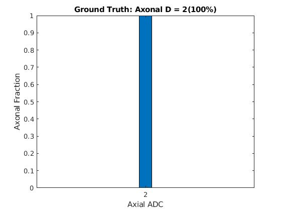
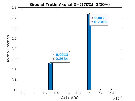
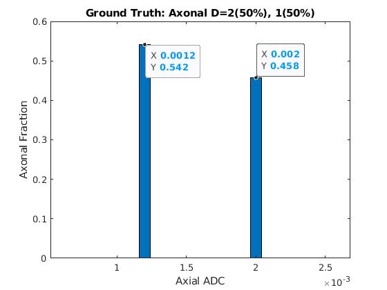
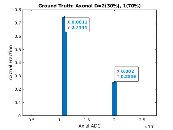
Figure 8: Axonal Health quantification using RADS. At the top of each plot is the simulated ground truth and the plots show the fractions recovered using RADS model.

We model the net anisotropic component of the signal as in Eq. 14 and solve as the minimization problem as in Eq. 17 for different values of unhealthy $\lambda_{\parallel}$, with $\lambda_{\parallel}=2$ for the healthy axons and $\lambda_{\perp}=0$. The model with the least BIC score is finally chosen. The results of the ‘Two component restricted anisotropic diffusion spectrum (RADS) model’ for quantifying Axonal Health are shown in Figure 8.

Our method produces highly accurate quantification of diseased and healthy axons with Pearson’s correlation (predicted vs true proportion) $r=0.99$ (p-value = 0.001); the one Sample t-test for proportion RMSE error gives the mean RMSE of 2% (p-value = 0.034). Furthermore, the method finds the axial diffusivities of the diseased and healthy axons very accurately with mean error of 4% (p-value = 0.001). For the Average vs predicted Average Axial ADC, we get the Pearson’s correlation (predicted vs true proportion) $r=0.98$ (p-value = 0.02). For the predicted Axial ADCs (predicted vs true ADCs), we get the Pearson’s correlation (predicted vs true proportion) $r=0.99$ (p-value $P<0.0001$).

5 Discussion

In the present work, we develop an extension of our previously developed method - DBSI- to quantify diseased axons in Multiple Sclerosis. The new method uses the anisotropic component of the diffusion-weighted signal to find the spectrum of axial diffusivities present in the anisotropic component. The modeling process is done in two steps. In the first step, we split the signal into its anisotropic and isotropic components and in the second step, the the anisotropic component of the signal is isolated and modeled as a linear combination of two parts - healthy and unhealthy axons based on the axial diffusivities. We developed a Monte-Carlo simulation package with the voxel geometry consisting of the three compartments - fiber compartment consisting of the uniformly spaced cylinders to model axons, the cell compartment consisting of uniformly spaced spheres to model cells, and the free water compartment. We run extensive MC simulations and validate our model. The first step of model recovers the fiber and cell fractions accurately with negligible variance, with Pearson’s correlation (predicted vs true proportion) of $r=0.999$ (p-value $<0.001$).

In the second step, we use two component restricted anisotropic diffusion spectrum (RADS) model to model the anisotropic component of the diffusion-weighted MRI signal. In this step, we model the anisotropic component as a linear combination of two parts - healthy and unhealthy axons based on the axial diffusivities. Bayesian information criterion (BIC) and model-fitting residuals were calculated to quantify model complexity and goodness of fit. Diffusion coefficients and signal fractions were computed for the optimal model (having lowest BIC). This gives us the fractions of diseased and healthy axons based on the axial diffusivities of the diseased and healthy axons. Using Monte-Carlo (MC) simulations, we simulate different fractions of diseased and healthy axons. Our method produces highly accurate quantification of diseased and healthy axons with Pearson’s correlation (predicted vs true proportion) of $r=0.99$ (p-value = 0.001); the one Sample t-test for proportion error gives the mean error of 2% (p-value = 0.034). Furthermore, the method finds the axial diffusivities of the diseased and healthy axons very accurately with mean error of 4% (p-value = 0.001).

References

- [1] Anderson AW. Measurement of fiber orientation distributions using high angular resolution diffusion imaging. Magn Reson Med., 54(5):1194–1206, 2005.
- [2] Matthew D. Budde, Mingqiang Xie, Anne H. Cross, and Sheng-Kwei Song. Axial diffusivity is the primary correlate of axonal injury in the experimental autoimmune encephalomyelitis spinal cord: A quantitative pixelwise analysis. Journal of Neuroscience, 29(9):2805–2813, 2009.
- [3] Pierpaoli C, Jezzard P, Basser PJ, Barnett A, and Di Chiro G. Diffusion tensor mr imaging of the human brain; 201(3). pages 637–648. Radiology, 1996.
- [4] Chia-Wen Chiang, Yong Wang, Peng Sun, Tsen-Hsuan Lin, Kathryn Trinkaus, Anne H. Cross, and Sheng-Kwei Song. Quantifying white matter tract diffusion parameters in the presence of increased extra-fiber cellularity and vasogenic edema. NeuroImage, 101:310–319, 2014.
- [5] A. Compston and A. Coles. Multiple sclerosis. Lancet (London, England), 359(9313):1221–1231, 2002.
- [6] A. Einstein. Über die von der molekularkinetischen theorie der wärme geforderte bewegung von in ruhenden flüssigkeiten suspendierten teilchen. Annalen der Physik, 322(8):549–560, 1905.
- [7] Charity Evans, Sarah-Gabrielle Beland, Sophie Kulaga, Christina Wolfson, Elaine Kingwell, James Marriott, Marcus Koch, Naila Makhani, Sarah Morrow, John Fisk, Jonathan Dykeman, Nathalie Jetté, Tamara Pringsheim, and Ruth Ann Marrie. Incidence and Prevalence of Multiple Sclerosis in the Americas: A Systematic Review. Neuroepidemiology, 40(3):195–210, 01 2013.
- [8] Joong Hee Kim, Matthew D. Budde, Hsiao-Fang Liang, Robyn S. Klein, John H. Russell, Anne H. Cross, and Sheng-Kwei Song. Detecting axon damage in spinal cord from a mouse model of multiple sclerosis. Neurobiology of Disease, 21(3):626–632, 2006.
- [9] Eric C. Klawiter, Robert E. Schmidt, Kathryn Trinkaus, Hsiao-Fang Liang, Matthew D. Budde, Robert T. Naismith, Sheng-Kwei Song, Anne H. Cross, and Tammie L. Benzinger. Radial diffusivity predicts demyelination in ex vivo multiple sclerosis spinal cords. NeuroImage, 55(4):1454–1460, 2011.
- [10] D.A. Lakhani, K.G. Schilling, J. Xu, and F. Bagnato. Advanced multicompartment diffusion mri models and their application in multiple sclerosis. American Journal of Neuroradiology, 41(5):751–757, 2020.
- [11] Marisa P. McGinley, Carolyn H. Goldschmidt, and Alexander D. Rae-Grant. Diagnosis and Treatment of Multiple Sclerosis: A Review. JAMA, 325(8):765–779, 02 2021.
- [12] R.T. Naismith, J. Xu, N.T. Tutlam, P.T. Scully, K. Trinkaus, A.Z. Snyder, S.-K. Song, and A.H. Cross. Increased diffusivity in acute multiple sclerosis lesions predicts risk of black hole. Neurology, 74(21):1694–1701, 2010.
- [13] R.T. Naismith, J. Xu, N.T. Tutlam, K. Trinkaus, A.H. Cross, and S.-K. Song. Radial diffusivity in remote optic neuritis discriminates visual outcomes. Neurology, 74(21):1702–1710, 2010.
- [14] Basser PJ, Mattiello J, and LeBihan D. Estimation of the effective self-diffusion tensor from the nmr spin echo. J Magn Reson B, 103(3):247–254, 1994.
- [15] Simona Schiavi, Maria Petracca, Peng Sun, Lazar Fleysher, Sirio Cocozza, Mohamed Mounir El Mendili, Alessio Signori, James S Babb, Kornelius Podranski, Sheng-Kwei Song, and Matilde Inglese. Non-invasive quantification of inflammation, axonal and myelin injury in multiple sclerosis. Brain, 144(1):213–223, 11 2020.
- [16] Gideon Schwarz. Estimating the dimension of a model. Ann. Statist., 6(2):461–464, 03 1978.
- [17] Afsaneh Shirani, Peng Sun, Robert E Schmidt, Kathryn Trinkaus, Robert T Naismith, Sheng-Kwei Song, and Anne H Cross. Histopathological correlation of diffusion basis spectrum imaging metrics of a biopsy-proven inflammatory demyelinating brain lesion: A brief report. Multiple Sclerosis Journal, 25(14):1937–1941, 2019. PMID: 29992856.
- [18] Sheng-Kwei Song, Shu-Wei Sun, Won-Kyu Ju, Shiow-Jiuan Lin, Anne H Cross, and Arthur H Neufeld. Diffusion tensor imaging detects and differentiates axon and myelin degeneration in mouse optic nerve after retinal ischemia. NeuroImage, 20(3):1714–1722, 2003.
- [19] Edward O Stejskal and John E Tanner. Spin diffusion measurements: spin echoes in the presence of a time-dependent field gradient. The journal of chemical physics, 42(1):288–292, 1965.
- [20] Peng Sun, Ajit George, Dana C. Perantie, Kathryn Trinkaus, Zezhong Ye, Robert T. Naismith, Sheng-Kwei Song, and Anne H. Cross. Diffusion basis spectrum imaging provides insights into ms pathology. Neurology - Neuroimmunology Neuroinflammation, 7(2), 2020.
- [21] Shu-Wei Sun, Hsiao-Fang Liang, Tuan Q. Le, Regina C. Armstrong, Anne H. Cross, and Sheng-Kwei Song. Differential sensitivity of in vivo and ex vivo diffusion tensor imaging to evolving optic nerve injury in mice with retinal ischemia. NeuroImage, 32(3):1195–1204, 2006.
- [22] Sun SW, Liang HF andTrinkaus K, Cross AH, Armstrong RC, and Song SK. Noninvasive detection of cuprizone induced axonal damage and demyelination in the mouse corpus callosum. Magn Reson Med, 55:302–8, 2006.
- [23] Amanuel Alemu Abajobir Valery L Feigin and et al. Kalkidan Hassen Abate. Global, regional, and national burden of neurological disorders during 1990–2015: a systematic analysis for the Global Burden of Disease Study 2015. Lancet Neurol. Nov; 16(11): 877–897., 16(11):877–897, Nov. 2017.
- [24] Marinus T. Vlaardingerbroek and Jacques A. den Boer. Magnetic Resonance Imaging: Theory and Practice, pages 67–68. Springer Berlin Heidelberg, Berlin, Heidelberg, 2003.
- [25] Mitchell T. Wallin, William J. Culpepper, Jonathan D. Campbell, Lorene M. Nelson, Annette Langer-Gould, Ruth Ann Marrie, Gary R. Cutter, Wendy E. Kaye, Laurie Wagner, Helen Tremlett, Stephen L. Buka, Piyameth Dilokthornsakul, Barbara Topol, Lie H. Chen, and Nicholas G. LaRocca. The prevalence of ms in the united states. Neurology, 92(10):e1029–e1040, 2019.
- [26] Yong Wang, Qing Wang, Justin P. Haldar, Fang-Cheng Yeh, Mingqiang Xie, Peng Sun, Tsang-Wei Tu, Kathryn Trinkaus, Robyn S. Klein, Anne Haney Cross, and Sheng-Kwei Song. Quantification of increased cellularity during inflammatory demyelination. Brain : a journal of neurology, 134 Pt 12:3590–601, 2011.