Estimating the Jet Power from Broadband SED modeling of Mkn 501 for different particle distributions

Abstract

We consider the broadband spectral energy distribution of the high energy peaked (HBL) blazar Mkn 501 using Swift-XRT/UVOT, NuSTAR and Fermi-LAT observations taken between 2013 and 2022. The spectra were fitted with a one-zone leptonic model using synchrotron and synchrotron self-Compton emission from different particle energy distributions such as a broken power-law, log-parabola, as well as distributions expected when the diffusion or the acceleration time scale are energy dependent. The jet power estimated for a broken power-law distribution was $\sim 10^{47}(10^{44})$ erg s^-1 for a minimum electron energy $\gamma_{\text{min}}\sim 10(10^{3})$. However, for electron energy distributions with intrinsic curvature (such as the log-parabola form), the jet power is significantly lower at a few times $10^{42}$ erg s^-1 which is a few percent of the Eddington luminosity of a $10^{7}$ M_⊙ black hole, suggesting that the jet may be powered by accretion processes. We discuss the implications of these results.

1 INTRODUCTION

Blazars are jetted objects, the subclass of Active Galactic Nuclei (AGN) where the jet is directly pointed towards the observer (Urry & Padovani, 1995b). Significant properties include its Spectral Energy Distribution (SEDs) ranging from Radio - TeV gamma rays, non-thermal radiation, rapid variability, radio-loud features, and double hump structure (Urry, 1998; Massaro et al., 2004a). Blazars are broadly classified into BL Lacs and Flat Spectrum Radio Quasars (FSRQs) based on their optical emission lines. FSRQs show strong emission lines in the optical band whereas BL Lacs show faint emission lines (Urry & Padovani, 1995a; Antonucci, 1993). Blazars are also classified into three classes based on the peak of the emission of the synchrotron component. For low-Energy peaked (LBL)/Low - Synchrotron peaked (LSP) BL Lacs, the low-energy hump peaks at the optical/UV band. For High energy peaked (HBL)/high synchrotron peaked (HSP) BL Lacs, the component peaks in the X-ray band and the Intermediate peaked BL Lacs (IBL) have a peak in between the X-rays and optical/UV band (Ghisellini et al., 1997; Fossati et al., 1998). The broadband SED is composed of two peaks with the lower one attributed to synchrotron emission. The radiative processes responsible for the second component in the high-energy regime are still unresolved. In the leptonic model interpretation, the component is assumed to be due to inverse Compton (IC) scattering (Dermer et al., 1992; Dermer & Schlickeiser, 1993). The seed photons for the IC processes may either be the synchrotron photons (i.e. the Synchrotron Self Compton (SSC) process) or they may be external photons from outside the jet (Marscher & Gear, 1985; Dermer & Schlickeiser, 1993; Khatoon et al., 2022).

One of the main challenges in understanding these systems, is the identification of the energy-generating process which results in these jets having such high powers, as inferred from broadband spectral fitting. For example, Paliya et al. (2017) have fitted the spectra of several blazars (both $\gamma$-ray loud and quiet) and have inferred total jet powers with an average value of few times $10^{47}$ erg s^-1 and with some sources exceeding $10^{48}$ erg s^-1. Such jet powers exceed the Eddington luminosity of super-massive black holes and hence they cannot be powered by accretion and instead require alternate energy production processes (e.g., Ghisellini et al. (2014)). In this interpretation, most of the jet power is in the kinetic energy of the protons whose number density is assumed to be the same as that of the non-thermal electrons. The inclusion of electron-positron pairs may decrease the power requirement, but it is unlikely that the pair fraction is substantial due to Compton drag effects and unobserved spectral signatures (e.g. Sikora & Madejski, 2000; Celotti & Ghisellini, 2008; Sikora et al., 2016). If instead of a leptonic origin for the VHE, one considers a hadronic one, then the jet power required is even higher and can exceed $10^{49}$ erg s^-1 (e.g. Zdziarski & Böttcher, 2015; Abe et al., 2023).

Since the jet power is dominated by the number of protons, the inferred jet power depends on the number of relativistic electrons. Typically the energy distribution of electrons is assumed to be a broken power-law form and the number of electrons then depends on the lowest lorentz factor of the distribution i.e. $\gamma_{\text{min}}$, which is often assumed to be of the order of unity or tens. Employing large values of $\gamma_{\text{min}}\sim 1000$, as permitted by the data can lead to a reduction in the jet power. However, the rationale behind having the minimum energy of the electrons to be that high remains unclear. Even then, assuming $\gamma_{\text{min}}=1000$, for the low flux state of Mkn 501, the jet power can still be as high as $\sim 10^{44}$ erg s^-1 (e.g. Abe et al., 2023).

The jet power estimations above have been primarily based on the assumption that the underlying electron energy distribution is a broken power-law (or a smoothened broken power-law). There have been some evidences based on the X-ray and $\gamma$-ray data that the observed spectrum has significant curvature deviating from a power-law (Massaro et al., 2004a; Tanihata et al., 2004; Tramacere, A. et al., 2007). This may indicate that the underlying electron energy distribution has a curvature which may have the shape of a log-parabola distribution (Massaro et al., 2004a). Physically motivated models have also been used such as distributions where the high energy cutoff is due to radiative losses ($\gamma$-max models), or where the curvature is due to energy-dependent acceleration (EDA) or energy-dependent diffusion (EDD) (Sinha et al., 2017; Goswami et al., 2018; Hota et al., 2021; Khatoon et al., 2022). Typically, these different interpretations are often spectrally degenerate, but perhaps may be distinguished by studying how physical are the observed correlations between the best fit spectral parameters for different models (Hota et al., 2021; Khatoon et al., 2022).

Electron energy distributions which are different from a broken power-law one, are expected to provide different estimates of the jet power. The motivation of this work is to estimate these different jet powers with statistical errors, by fitting a set of broadband SED of a bright blazar, with models having different electron distributions. To do this, we consider the HBL source Mkn 501 at a redshift of z = 0.034 which is among the most well studied blazars with VHE emission. It shows extreme HBL characteristics during flaring as reported by Ahnen, M. L. et al. (2018) and Sahu et al. (2020). It was first detected in 1995 by the Whipple observatory (Quinn et al., 1996). It is one of the brightest blazar sources in the catalog after Mkn 421, and has been studied through several multi-wavelength missions. Moreover, Mkn 501 shows significant curvature in the SED as investigated by Tavecchio et al. (2001), which may be described by a log parabola distribution (Massaro et al., 2004b). As reported by Abe et al. (2023), during 15 years of swift observations, the Swift-XRT flux rate was high from 2012 to 2014, with the highest X-ray flaring activity during March-October 2014. A recent multi-wavelength study by Furniss et al. (2015) with NuSTAR observations reported hard X-ray variability in the timescale $\sim$ 7 hours in the range from 7-30 keV which was not previously observed. For this work, we analyzed multi-wavelength observations from Swift-XRT/UVOT, NuSTAR, and Fermi-LAT during the period from 2013 to 2022 covering the high and historically low activity state of Mkn 501, giving ten near simultaneous broadband SED, which we fit using different models. The section 2 describes the observations and the data analysis technique. In section 3, the broadband spectral analysis is reported, whose results are presented in section 4. We summarise and discuss the results in the section 5. In this work, the cosmological constant is considered in accordance with the $\Lambda$CDM model with $H_{0}$ = 71 km s^-1 Mpc ^-1, $\Omega_{\Lambda}=0.73$, $\Omega_{M}=0.27$ (Komatsu et al., 2011).

2 Observations and Data Analysis

2.1 NuSTAR

Nuclear Spectroscopic Telescope Array (NuSTAR) is a space-based X-ray telescope used for nuclear spectroscopy. It was launched by NASA on 13 June 2012 which uses a Wolter Telescope. It consists of two Focal Plane modules FPMA and FPMB (Harrison et al., 2013). Several observations of Mkn 501 were obtained between 2013 to 2022 which are summarized in Table 1.

The software package, "nupipeline" which is integrated with Heasoft-6.28, has been used for the generation of cleaned data files for the analysis. "XSELECT V2.4k" was used for plotting the event fits files (cl.evt) in ds9. Source extraction of 30 arcseconds and background of 60 arcseconds had been carried out for all the NuSTAR observations. The "nuproducts" tool was used for the generation of spectrum files (PHA), ancillary files (ARF), and response matrix files (RMF). The "grppha" tool was used to obtain the grouped spectra with all the obtained products to have counts of 30 per bin.

2.2 Swift-XRT

We considered observations undertaken by Swift-XRT which are nearly simultaneous with the NuSTAR ones. The detector has an area of 135 cm² covering an energy range of (0.2 - 10 keV). Observations for the instruments NuSTAR and Swift-XRT are provided by NASA’s HEASARC archive. Corresponding to the NuSTAR observation during March 2022, there are two Swift-XRT observations for which the analysis was carried out separately i.e. without summing the two Swift-XRT spectra. The observation details are listed in Table 1.

We have used the software package "xrtpipeline" which is integrated with Heasoft-6.28, for the generation of cleaned data and used "XSELECT V2.4K" for plotting the event fits files (cl.evt) in ds9. For the observations taken during 2013, 2021, and 2022 the Swift-XRT counts were comparatively higher than the ones during 2017 and 2018. Among the 10 observations, 9 observations of Swift-XRT are in the Windowed Timing (WT) mode, which are free from pile-up. For all the non-piled-up observations, a source region of 10 pixels and a background region of 20 pixels are extracted. However, "Obs ID 00035023170" was found to be piled up since it is in the "photon counting" (PC) mode. For this observation, we extracted an annular region with an inner radius of 7 pixels and an outer radius of 18 pixels, and a background region of 36 pixels which was free from source contamination. Using "XSELECT V2.4k", the light curve and spectrum are extracted, and using "xrtmkarf" and "quzcif" tools the ancillary (ARF) and response matrix files (RMF) were generated respectively. Like NuSTAR, Swift-XRT spectrum was grouped such that there were at least 30 counts per bin.

2.3 Swift-UVOT

The UV observations for the data sets were taken from Swift-UVOT. The Swift-UVOT covers both the optical and UV bands of the EM spectrum and consists of three optical filters (B, V, U) and three UV filters (uvw1, uvw2, uvm2) (Roming et al., 2005). However, for the observations under consideration, only the UV filters were available. The source and background regions of 8 arcsecs and 16 arcsecs were extracted. The tool "UVOTSOURCE" was used to calculate the magnitude in the AB magnitude system. We have used the relation $\frac{A_{v}}{E(B-V)}=3.1$ for the magnitude correction, where A_v is the galactic extinction and $E(B-V)$ is the interstellar reddening which has been taken to be 0.017 mag (Schlafly & Finkbeiner, 2011).

From the magnitude values, the flux was calculated with the help of photometric zero points and conversion factors adopted from Breeveld et al. (2011); Larionov et al. (2016). The flux points and energies of UVOT observations were converted to "XSPEC version 12.11.1" (Arnaud, 1996) readable (PHA) format using the tool "ftflx2xsp".

2.4 Fermi-LAT

The Large Area Telescope onboard the Fermi Gamma-ray Space Telescope Fermi-LAT, operates in the energy range from 20 MeV to more than 300 GeV (Atwood et al., 2009). In order to get a significant detection and spectra, we considered the 4 months Fermi-LAT observations keeping the NuSTAR observations in the middle of the total duration. We analyzed the data spanning from February 2013 to May 2022 using the open-source tools fermipy . We considered the region of interest (ROI) to be 15^∘ to carry out the analysis and followed the standard procedure as mentioned in the documentation (Wood et al., 2017). The energy range considered was from 100 MeV to 300 GeV with evclass=128 and evtype=3. The latest instrument function (IRF) "P8R3 SOURCE V3" has been used. To generate XML files, the galactic diffusion "gll iem v07.fits" and the isotropic background model "iso P8R3 SOURCE V3 v1.txt" have been used. Using the latest Fermi-LAT 4FGL catalog (Abdollahi et al., 2020), we have acquired the XML model file encompassing all sources within the ROI. Along with it, the fourth Fermi source catalog providing the spectral models and parameters for the sources located within the ROI are considered. Finally, the flux points and energies of Fermi-LAT observations are converted to XSPEC readable (PHA) format using the tool "ftflx2xsp".

Table 1: Summary of NuSTAR and Swift-XRT/UVOT observations of the source Mkn 501.

NuSTAR Swift-XRT / UVOT Obs ID Date and Time MJD Exposure (ks) Obs ID Date and Time Exposure (XRT) (ks) Exposure (UVOT) (ks) S₁ 60002024002 2013-04-13 T02:31:07 56395 18.27 00080176001 2013-04-13 T01:20:59 9.65 9.46 S₂ 60002024006 2013-07-12 T21:31:07 56485 10.85 00030793233 2013-07-12 T00:54:59 1.02 1.01 S₃ 60002024008 2013-07-13 T20:16:07 56486 10.34 00030793236 2013-07-13 T07:20:58 1.01 1.00 S₄ 60202049002 2017-04-27 T22:26:09 57870 23.15 00035023156 2017-04-27 T23:02:56 1.07 1.06 S₅ 60202049004 2017-05-24 T22:11:09 57897 23.83 00035023170 2017-05-24 T07:58:57 0.96 0.95 S₆ 60466006002 2018-04-19 T15:06:09 58227 23.11 00035023212 2018-04-19 T22:19:57 1.00 0.98 S₇ 60702062002 2021-07-13 T17:36:09 59408 20.63 00011184138 2021-07-12 T22:39:35 0.81 0.80 S₈ 60701032002 2022-03-09 T10:01:09 59647 19.72 00011184179 2022-03-09 T02:58:36 0.99 0.97 S₉ 60701032002 2022-03-09 T10:01:09 59647 19.72 00011184180 2022-03-09 T22:19:57 1.02 1.01 S₁₀ 60702062004 2022-03-27 T01:26:09 59665 20.29 00011184187 2022-03-27 T03:49:36 0.93 0.92

3 Broadband Spectral Analysis

The source Mkn 501 is well known to have the X-ray emission from synchrotron radiation, however, the hump in the higher energy is attributed mainly to the inverse Compton (IC) process. In our broadband spectral fitting of Mkn 501, we have considered the leptonic model with a single emitting region. We assume a spherical region having a radius R, filled with a tangled magnetic field, B, and isotropic electron distribution, n($\gamma$), moving with bulk lorentz factor $\Gamma$ at an angle $\theta$ with respect to the observer’s direction. The seed photons of the IC process are the synchrotron photons i.e. the synchrotron self-Compton (SSC) process. We fit the broadband using a local model in XSPEC as described below. For the spectral fit, we have used the "Tbabs" model (Wilms et al., 2000) to account for the Galactic absorption. The hydrogen column density for the X-ray observations, ${N_{\text{H}}}=1.69\times 10^{20}$ $\text{cm}^{-2}$ was considered and kept fixed, which was obtained in the LAB survey (Kalberla et al., 2005). However, for the UV the $N_{\text{H}}$ value was fixed at 0 since the UV flux was dereddened initially. For error calculation, we have adopted Markov Chain Monte Carlo (MCMC) method using the python-based code XSPEC_EMCEE. We have used 50 walkers with 5000 iterations and burnt the first 2000. The errors were calculated within a confidence range of 2$\sigma$. EMCEE is an extensible, pure-Python implementation of Goodman & Weare’s Affine Invariant Markov chain Monte Carlo (MCMC) Ensemble sampler.

Since the objective is to fit the broadband spectra with different electron energy distributions, $n(\gamma)$, it is convenient to use a convolution model in XSPEC such that it can be used along with a function that represents the electron distribution. In particular, we follow Hota et al. (2021); Khatoon et al. (2022) to represent the synchrotron flux at an energy $\epsilon$ to be,

$$F_{\text{syn}}(\epsilon)=\frac{\delta^{3}(1+z)}{d_{L}^{2}}V\mathbb{A}\int_{\xi_{\text{min}}}^{\xi_{\text{max}}}f\left(\frac{\epsilon}{\xi^{2}}\right)n(\xi)d\xi$$ (1)

where $d_{L}$ is the luminosity distance and V is the volume of the emission region, $\mathbb{A}=\frac{\sqrt{3}\pi e^{3}B}{16m_{e}c^{2}\sqrt{C}}$ and $f(x)$ is the synchrotron emissivity function. Instead of using the electron’s lorentz factor $\gamma$, the electron energy distribution is represented by $n(\xi)$. The transformation is given by $\xi=\gamma\sqrt{\mathbb{C}}$, where $\mathbb{C}=1.36\times 10^{-11}\frac{\delta B}{1+z}$ keV with $\delta$ as the doppler factor, B as the magnetic field, and z being the redshift of the source. Note that $\xi$ represents $\gamma$ and $\xi^{2}$ has dimension of keV. Similarly, the synchrotron self-Comptonization flux is determined as a function of $F_{\text{syn}}(\epsilon)$ and $n(\xi)$. The expressions used for the flux are given in Sahayanathan et al. (2018) and references therein, with $\gamma$ transformed to $\xi$. Thus we have a local XSPEC convolution model, sscicon. which can be convolved with any particle distribution using the XSPEC model form (sscicon*n($\xi$)). The convolution model sscicon has the following parameters, bulk lorentz factor $\Gamma$, redshift $z$, magnetic field $B$, viewing angle $i$, and size $R$. The other parameters including normalization $K$, arise from the specific particle distribution form as described below. The model has the provision to have as a parameter, the jet power $P_{\text{j}}$, instead of normalization, $K$. We describe the different particle distributions used in this work below.

3.1 Logparabola model

We consider the particle density to be described by the log parabola function,

$$n({\xi})=K\left(\frac{\xi}{\xi_{r}}\right)^{-\alpha-\beta\text{log}\left(\frac{\xi}{\xi_{r}}\right)}$$ (2)

Here, particle spectral index is $\alpha$ at the reference energy $\xi_{r}$, while $\beta$ and $K$ are the spectral curvature parameter and the normalization. The reference $\xi_{r}^{2}$ was fixed at 1 keV during the spectral fit and the other three parameters $\alpha,\beta$ and norm $K$ were kept free.

3.2 Broken Power Law

We considered a Broken power law (BPL) distribution of the particles to fit the spectrum.

$$n(\xi)=\begin{cases}K(\xi/1\sqrt{{\text{keV}}})^{-p}&\text{for}\hskip 3.0pt\xi<\xi_{\text{break}}\\ K\xi^{q-p}_{\text{break}}(\xi/1\sqrt{{\text{keV}}})^{-q}&\text{for}\hskip 3.0pt\xi>\xi_{\text{break}}\end{cases}$$ (3)

Where $\xi_{\text{break}}$ is the break energy, p is the electron spectral index for $\xi$ < $\xi_{\text{break}}$ and q is the electron spectral index for $\xi>\xi_{\text{break}}$ and the transformation is given by $\xi=\gamma\sqrt{\mathbb{C}}$. We consider the broken power-law particle distribution to exist only between a minimum and maximum $\gamma$ i.e. $n(\xi)$ is non-zero for $\xi_{\text{min}}<\xi<\xi_{\text{max}}$, where $\xi_{\text{min}}=\gamma_{\text{min}}\sqrt{\mathbb{C}}$ and $\xi_{\text{max}}=\gamma_{\text{max}}\sqrt{\mathbb{C}}$.

3.3 Particle distribution with a maximum electron energy

We consider the case where there is acceleration and electrons lose energy through the radiative processes. The evolution of the particles in the acceleration region is governed by the kinetic equation which is given by,

$$\scriptsize\frac{\partial}{\partial\gamma}\left[\left(\frac{\gamma}{\tau_{\text{acc}}}-\beta_{s}\gamma^{2}\right)n_{a}\right]+\frac{n_{a}}{\tau_{\text{esc}}}=Q\delta(\gamma-\gamma_{0})$$ (4)

Where the $\tau_{\text{acc}}$ and $\tau_{esc}$ are the acceleration and escape time scales of the electrons. $\beta_{s}$ is the cooling term is given by, $\beta_{s}=\frac{4}{3}\frac{\sigma_{T}B^{2}}{8\pi m_{e}c^{2}}$, where B is the magnetic field, $\sigma_{T}$ is the Thomson’s cross-section, and $m_{e}$ is the mass of the electron. Q is the mono-energetic injection of electrons at minimum energy $\gamma_{0}$. The solution is given by,

$$\scriptsize n(\xi)=K\xi^{-p}(1-(\xi/\xi_{\text{max}}))^{(p-2)}$$ (5)

where, $p=\frac{\tau_{\text{acc}}}{\tau_{\text{esc}}}+1$, $\xi_{\text{max}}=\gamma_{\text{max}}\sqrt{\mathbb{C}}$, $\gamma_{\text{max}}=\frac{1}{\beta_{s}\tau_{\text{acc}}}$

The particle distribution exists only for $\xi>\xi_{\text{min}}$, where $\xi_{\text{min}}=\gamma_{\text{min}}\sqrt{\mathbb{C}}$ .

3.4 Energy dependent time-scale models:

We also employed models incorporating energy-dependent escape or acceleration timescales to provide a possible interpretation of the curvature in the observed spectrum (Hota et al., 2021; Khatoon et al., 2022).

3.4.1 Energy dependent diffusion model (EDD)

The diffusion takes place within a region containing a tangled magnetic field, causing the escape time scale to depend on the electron’s gyration radius. In this context, the escape time scale ($\tau_{\text{esc}}$) maybe energy dependent as

$$\tau_{esc}=\tau_{esc,R}\left(\frac{\gamma}{\gamma_{R}}\right)^{-k}$$ (6)

where, $\tau_{esc,R}$ corresponds to $\tau_{esc}$, when the electron energy is $\gamma_{R}mc^{2}$, and $k$ is the index of the assumed power-law energy dependence. As $\gamma_{R}$ cannot be greater than the free streaming value $\tau_{esc,R}$ which restricts the equation to $\gamma<\gamma_{R}$, where $\gamma_{R}$ denotes the energy at which this limit is obtained. If we make the assumption that $\gamma_{R}$ is significantly greater than any $\gamma$ of interest and ignore the synchrotron losses, we obtain the following electron energy distribution,

$$n(\xi)=Q_{0}\tau_{acc}\sqrt{\mathbb{C}}\xi^{-1}exp\left[-\frac{n_{R}}{k}\left(\left(\frac{\xi}{\xi_{R}}\right)^{k}-\left(\frac{\xi_{0}}{\xi_{R}}\right)^{k}\right)\right]$$ (7)

where, $\xi_{R}=\sqrt{\mathbb{C}}\gamma_{R}$, $\xi_{0}=\sqrt{\mathbb{C}}\gamma_{0}$ and $\eta\equiv\frac{\tau_{acc}}{\tau_{esc,R}}$

It is convenient to recast the distribution as follows,

$$n(\xi)=K(\xi)^{-1}exp\left[-\frac{\psi}{k}\xi^{k}\right]$$ (8)

with $K$, $\psi$, and $k$ representing the free parameters. It can be shown that,

$$\psi=\eta_{R}(\mathbb{C}\gamma^{2}_{R})^{-k/2}=\eta_{R}\xi_{R}^{-k}$$

and that the normalization is given by,

$$K=Q_{0}\tau_{acc}\text{exp}\left[\frac{n_{R}}{k}\left(\frac{\xi_{0}}{\xi_{R}}\right)^{k}\right]$$

3.4.2 Energy dependent acceleration (EDA) model

We consider the prospect that acceleration time-scale is energy-dependent and we assume its functional form to be given by,

$$\tau_{acc}=\tau_{acc,R}\left(\frac{\gamma}{\gamma_{R}}\right)^{k}$$ (9)

Where, $\tau_{acc,R}$ corresponds to $\tau_{acc}$, when the electron energy is $\gamma_{R}mc^{2}$ and $k$ is the index of the energy dependence. Similar to the case of the EDD model, the corresponding electron energy distribution is given by,

$$\scriptsize n(\xi)=Q_{0}\tau_{acc}\sqrt{\mathbb{C}}\xi_{R}^{-k}\xi^{k-1}\text{exp}\left[-\frac{n_{R}}{k}\left(\left(\frac{\xi}{\xi_{R}}\right)^{k}-\left(\frac{\xi_{0}}{\xi_{R}}\right)^{k}\right)\right]$$ (10)

which can be recast as,

$$\scriptsize n(\xi)=K(\xi)^{k-1}\text{exp}\left[-\frac{\psi}{k}\xi^{k}\right]$$ (11)

where,

$$\psi=\eta_{R}(\mathbb{C}\gamma^{2}_{R})^{(-k/2)}=\eta_{R}\xi_{R}^{-k}$$

K is the normalization which is given by,

$$K=Q_{0}\tau_{acc}\xi_{R}^{-k}\text{exp}\left[\frac{n_{R}}{k}\left(\frac{\xi_{0}}{\xi_{R}}\right)^{k}\right]$$

4 Results

We performed the fitting of the observations listed in Table 1 using the various particle distributions discussed in the preceding section. We fixed the bulk lorentz factor, $\Gamma=15$, and the viewing angle, $i=0$, and allowed for the other parameters to vary. Note that for synchrotron and synchrotron-self Compton processes considered here, the relevant parameter is the doppler factor $\delta=1/(\Gamma(1-\beta\text{cos}i)$ which for $i=0$, $\delta=2\Gamma$.

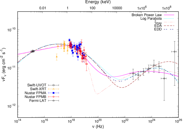
Figure 1: Broadband SED plot of the observation s4 (MJD 57870) of Mkn 501 for all the five particle distribution models.

For observations made during 2013 (listed as S₂ and S₃ in Table 1), none of the models considered provided a reasonable fit. This was because the Swift-XRT spectra seemed to have a high energy excess, incompatible with the NuSTAR spectra. We were unable to find the reason for this and diferred a more detailed investigation of this to a later work. Thus, for these two observations, the Swift-XRT spectra were omitted. Using the different particle distributions, we achieved reasonable fits for all ten broadband spectra, and the corresponding best-fit parameters are listed in Table 2. A representative spectrum for the observation during MJD 57870 ( listed as S₄ in Table 1) is shown in Figure 1, with the different best-fit model spectra overlayed. For some of the observations, especially the latter ones during 2022, the broken power-law distribution provides a better fit than the others. We note that the majority of the $\chi^{2}$ contribution originates from the X-ray spectra and in general for all the particle distribution considered, broadband SED is reasonably represented.

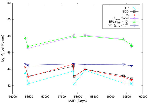
Figure 2: Variation of jet power for different particle distribution models.

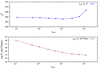
Figure 3: Variation of $\chi^{2}$ (top panel) and Jet Power (bottom panel) with $\gamma_{\text{min}}$ for the observation (MJD 57870) for BPL particle distribution.

The estimated jet power differs significantly for the different particle distributions as shown in Figure 2 where the jet power is plotted against MJD. The models that have intrinsic curvature in the particle energy distributions (i.e. log-parabola, EDD and EDA) require nearly two orders of magnitude less jet power than the broken power-law and gamma-max distributions. For the latter two distributions, the jet power depends sensitively on the minimum energy of the electrons, $\gamma_{\text{min}}$. Figure 3 shows the variation of $\chi^{2}$ (top panel) and jet power as a function of $\gamma_{\text{min}}$ for the broken power-law distribution for a representative data set. As expected the jet power decreases with increasing $\gamma_{\text{min}}$ for large values, the $\chi^{2}$ increases because the UV flux is no longer consistent. For a value as large as $\gamma_{\text{min}}\sim 10^{3}$, the jet power for the broken power-law model is $\sim 10^{44}$ erg s^-1, which is still significantly larger than the power estimated for the log-parabola model in Figure 2.

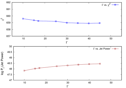
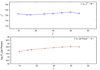
Figure 4: Variation of $\chi^{2}$ (Top panel) and Jet Power (bottom panel) with $\Gamma$ for the observation (MJD 57870) for BPL (left panel) and LP (right panel) particle distribution.

In the above analysis, it was assumed that the bulk lorentz factor $\Gamma=15$. For a representative data set, the top panels of Figure 4 show the variation of $\chi^{2}$ as a function of $\Gamma$ for the broken power-law (left panel) and log-parabola (right panel) models. The bottom panels show the dependence of jet power with $\Gamma$. As can be seen, $\Gamma$ is not constrained since the $\chi^{2}$ does not change with increasing $\Gamma$. The jet power increases with $\Gamma$ but only marginally, a factor of two increase when $\Gamma$ increases from 10 to 45. Thus the broad estimates of the jet powers presented here with $\Gamma=15$ are not sensitive to that assumption.

5 Summary and Conclusions

We collated ten broadband spectral energy distributions for Mkn 501, spanning 2013 to 2022, using data from Swift-UVOT, Swift-XRT, NuSTAR, and Fermi-LAT. We fitted the broad band spectra using a single zone leptonic model taking into account synchrotron and synchrotron-self Compton emission from a non-thermal electron distribution. Different electron energy distributions were considered such as a broken power-law, power-law with a maximum energy due to radiative cooling ($\gamma$-max model), log-parabola, energy-dependent diffusion time-scale (EDD) and energy-dependent acceleration time-scale (EDA). We determined that all these models adequately explained the broadband spectra and may be considered spectrally degenerate.

We estimated the total jet power with errors for the different observations and for different particle energy distributions. We found as reported before, that the jet power for broken power-law and $\gamma$-max models, was as high as $\sim 10^{47}$ erg s^-1 for a minimum lorentz factor $\gamma_{\text{min}}=10$ and reduced to $\sim 10^{44}$ erg s^-1 for $\gamma_{\text{min}}=10^{3}$, which was the maximum value allowed for spectral fitting. On the other hand, for the other energy particle distributions with intrinsic curvature, the jet power turned out to be $\sim 10^{43}$ erg s^-1, independent of $\gamma_{\text{min}}$. We show that these estimates for jet power are nearly independent of the chosen value of the bulk lorentz factor $\Gamma$.

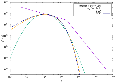
Figure 5: Particle energy distributions for the observation s3 (MJD 56486).

To illustrate the reason for the difference in jet power among various particle distributions, we plotted Figure 5 that shows the particle distributions $\gamma^{2}n(\gamma)$ as a function of $\gamma$ for the broken power-law, log-parabola, EDA, and EDD models for observation S₃. The peak of the function indicates the energies at which most of the particle energy dominates. In the case of the broken power-law distribution, the peak occurs at $\gamma_{\text{min}}$ and is significantly higher than for the other distributions, resulting in a higher jet power. It’s noteworthy that the X-ray emission at $\sim$ 1 keV arises from electrons with $\gamma$ values of $\sim$ 1.6 × 10⁶, 7.5 × 10⁴, 1.25 × 10⁵, and 1.25 × 10⁵ for the broken power-law, log-parabola, EDA, and EDD models, respectively.

The comparatively lower jet power estimated for the intrinsically curved particle energy distributions (especially the log-parabola one) of $\sim 10^{43}$ erg s^-1 makes it about a few percent of the Eddington luminosity for a $10^{7}$ M_⊙ blackhole, $L_{\text{Edd}}\sim 10^{45}$ erg s^-1. This has an important ramification that such a jet may be directly powered by the accretion process, which in turn may provide a framework to understand the jet-disc connections inferred from the correlation between disc and jet parameters in non-beamed systems (Cao & Jiang, 1999; Ho & Peng, 2001; Ghisellini et al., 2014; Sbarrato et al., 2016). Furthermore, the results will have a bearing on galaxy evolution studies which invoke AGN feedback through a powerful jet (Fabian, 2012; Cielo et al., 2018). A low jet power also indicates a smaller reservoir of energy in the jet, which may be depleted due to shocks and radiative losses in a shorter time scale. This provides an incentive to make a detailed study of the time evolution of such systems that have intrinsically curved particle distributions and hence lower jet power.

The intrinsically curved particle distributions assumed in this work, are empirical in the sense that the curvature is due to an assumed energy dependence of the diffusion or acceleration time-scales. Clearly, a more detailed study considering the micro-physics of the processes needs to be undertaken to validate the assumed dependence. Finally, the analysis needs to be extended to different blazars, especially other kinds of blazars, such as FSRQs, to get a more comprehensive picture.

DATA AVAILABILITY

The data and software used in this study can be accessed via NASA’s HEASARC webpages and the Fermi Science Support Center (FSSC), for which the corresponding links and references are provided within the manuscript.

Table 2: The table reports the best-fitting spectral parameters obtained by fitting the broadband spectrum with the one-zone leptonic model with various particle distributions. For all the models the bulk Lorentz factor is fixed at, $\Gamma=15$. The magnetic field is in the units of Gauss (G), Radius of the emitting region R and Jet Power $P_{j}$ are in logarithmic scale with the units of cm and erg s^-1. For the BPL distribution, $\xi_{\text{max}}=10^{5}$ $\sqrt{\text{keV}}$ and $\xi_{\text{min}}=10^{-5}$ $\sqrt{\text{keV}}$, and for $\xi_{\text{max}}$ distribution,$\xi_{\text{min}}=10^{-5}\sqrt{\text{keV}}$ have been considered.

				Log Parabola
	Obs	$\alpha$	$\beta$	B (G)	log R(cm)	log $P_{j}$	$\chi^{2}_{\text{red}}(\text{dof})$
	S1	3.09${}^{+0.01}_{-0.01}$	0.32${}^{+0.01}_{-0.01}$	0.043${}^{+0.01}_{-0.01}$	15.9${}^{+0.01}_{-0.08}$	43.55${}^{+0.02}_{-0.02}$	1.06 (847)
	S2	2.77${}^{+0.01}_{-0.01}$	0.45${}^{+0.02}_{-0.02}$	0.68${}^{+0.30}_{-0.04}$	15${}^{+0.18}_{-0.18}$	42.38${}^{+0.002}_{-0.002}$	1.04 (680)
	S3	2.81${}^{+0.01}_{-0.01}$	0.48${}^{+0.02}_{-0.02}$	3.16${}^{+1.07}_{-0.2}$	14.44${}^{+0.08}_{-0.08}$	42.20${}^{+0.001}_{-0.001}$	1.04(634)
	S4	3.08${}^{+0.01}_{-0.01}$	0.25${}^{+0.02}_{-0.02}$	0.39${}^{+0.27}_{-0.29}$	15.26${}^{+0.96}_{-1.2}$	44.03${}^{+0.003}_{-0.003}$	1.19 (605)
	S5	3.81${}^{+0.04}_{-0.03}$	0.79${}^{+0.06}_{-0.05}$	0.048${}^{+0.02}_{-0.004}$	16.03${}^{+0.007}_{-0.14}$	42.23${}^{+0.1}_{-0.06}$	1.04 (294)
	S6	3.17${}^{+0.04}_{-0.04}$	0.24${}^{+0.01}_{-0.01}$	0.0063${}^{+0.07}_{-0.006}$	16.83${}^{+0.66}_{-2.04}$	43.85${}^{+0.6}_{-0.47}$	0.88 (201)
	S7	3.34${}^{+0.01}_{-0.01}$	0.62${}^{+0.01}_{-0.01}$	1.52${}^{+2.03}_{-0.77}$	14.67${}^{+0.19}_{-0.32}$	42.30${}^{+0.06}_{-0.07}$	1.18 (540)
	S8	3.04${}^{+0.01}_{-0.01}$	0.61${}^{+0.02}_{-0.02}$	1.19${}^{+1.2}_{-0.58}$	14.82${}^{+0.4}_{-0.5}$	42.3${}^{+0.06}_{-0.07}$	1.68 (791)
	S9	3.05${}^{+0.01}_{-0.01}$	0.63${}^{+0.02}_{-0.02}$	1.58${}^{+1.16}_{-0.87}$	14.72${}^{+0.44}_{-0.44}$	42.18${}^{+0.16}_{-0.03}$	1.55 (797)
	S10	2.86${}^{+0.01}_{-0.01}$	0.5${}^{+0.02}_{-0.02}$	1.55${}^{+0.16}_{-0.28}$	14.77${}^{+0.24}_{-0.53}$	42.27${}^{+0.14}_{-0.03}$	1.57 (956)
				Broken power law
Obs	p	q	$\xi_{\text{break}}$ $\sqrt{\text{(keV)}}$	B (G) (10-3)	log R(cm)	log $P_{j}$	$\chi^{2}_{\text{red}}(\text{dof})$
S1	2.76${}^{+0.01}_{-0.01}$	3.64${}^{+0.02}_{-0.05}$	1.5${}^{+0.07}_{-0.07}$	1.8${}^{+0.002}_{-0.0004}$	17.49${}^{+0.57}_{-0.51}$	47.7${}^{+0.003}_{-0.003}$	1.06 (846)
S2	2.41${}^{+0.02}_{-0.03}$	3.72${}^{+0.16}_{-0.15}$	2.44${}^{+0.26}_{-0.26}$	1.1${}^{+0.26}_{-0.02}$	17.5${}^{+0.0008}_{-0.12}$	46.6${}^{+0.002}_{-0.002}$	1.08 (679)
S3	2.43${}^{+0.03}_{-0.02}$	3.88${}^{+0.49}_{-0.24}$	2.52${}^{+0.44}_{-0.29}$	1.0${}^{+0.0008}_{-0.0008}$	17.49${}^{+0.01}_{-0.17}$	46.75${}^{+0.003}_{-0.003}$	1.008(633)
S4	2.86${}^{+0.02}_{-0.02}$	3.99${}^{+0.42}_{-0.36}$	2.58${}^{+0.50}_{-0.54}$	3.7${}^{+0.001}_{-0.002}$	17.32${}^{+0.6}_{-0.8}$	48.01${}^{+0.05}_{-0.07}$	1.09 (604)
S5	2.81${}^{+0.05}_{-0.05}$	4.57${}^{+0.15}_{-0.12}$	0.98${}^{+0.13}_{-0.11}$	2.02${}^{+0.001}_{-0.0002}$	17.50${}^{+0.01}_{-0.15}$	47.8${}^{+0.03}_{-0.03}$	0.94 (293)
S6	2.94${}^{+0.03}_{-0.03}$	4.69${}^{+0.16}_{-0.1}$	0.88${}^{+0.08}_{-0.03}$	1.21${}^{+0.0005}_{-0.0005}$	17.86${}^{+0.12}_{-0.25}$	48.01${}^{+0.003}_{-0.003}$	0.93 (200)
S7	2.69${}^{+0.02}_{-0.03}$	4.23${}^{+0.11}_{-0.12}$	1.46${}^{+0.11}_{-0.13}$	2.40${}^{+0.001}_{-0.0001}$	17.30${}^{+0.004}_{-0.24}$	47.61${}^{+0.03}_{-0.003}$	1.06 (539)
S8	2.51${}^{+0.02}_{-0.02}$	4.37${}^{+0.16}_{-0.14}$	1.95${}^{+0.09}_{-0.1}$	4.64${}^{+0.003}_{-0.0003}$	17.01${}^{+0.003}_{-0.26}$	46.9${}^{+0.003}_{-0.03}$	1.13 (790)
S9	2.49${}^{+0.02}_{-0.02}$	4.3${}^{+0.36}_{-0.13}$	1.86${}^{+0.26}_{-0.1}$	1.24${}^{+0.001}_{-0.0001}$	17.5${}^{+0.001}_{-0.45}$	46.9${}^{+0.003}_{-0.03}$	1.06 (796)
S10	2.45${}^{+0.01}_{-0.01}$	4.03${}^{+0.11}_{-0.10}$	2.19${}^{+0.11}_{-0.1}$	1.07${}^{+0.0002}_{-0.0005}$	17.5${}^{+0.06}_{-2.25}$	46.7${}^{+0.003}_{-0.003}$	1.07 (955)
				$\xi_{\text{max}}$
	Obs	p	$\xi_{\text{max}}$ $\sqrt{\text{(keV)}}$	B (G) (10-3)	log R(cm)	log $P_{j}$	$\chi^{2}_{\text{red}}(\text{dof})$
	S1	2.76${}^{+0.03}_{-0.03}$	6.09${}^{+0.35}_{-0.35}$	2.1${}^{+0.009}_{-0.001}$	17.5${}^{+0.008}_{-0.22}$	47.8${}^{+0.003}_{-0.003}$	1.09 (847)
	S2	2.41${}^{+0.01}_{-0.01}$	6.61${}^{+0.27}_{-0.23}$	1.0${}^{+0.0005}_{-0.0005}$	17.5${}^{+0.0008}_{-0.12}$	46.74${}^{+0.003}_{-0.003}$	1.04 (680)
	S3	2.36${}^{+0.03}_{-0.02}$	7.9${}^{+0.47}_{-0.36}$	3.2${}^{+0.002}_{-0.0003}$	16.99${}^{+0.002}_{-0.32}$	46.5${}^{+0.003}_{-0.003}$	1.01(634)
	S4	2.81${}^{+0.01}_{-0.01}$	8.48${}^{+0.5}_{-0.48}$	2.2${}^{+0.001}_{-0.002}$	17.49${}^{+0.66}_{-1.05}$	47.9${}^{+0.003}_{-0.003}$	1.09 (605)
	S5	2.91${}^{+0.02}_{-0.01}$	3.76${}^{+0.1}_{-0.1}$	1.0${}^{+0.0005}_{-0.0005}$	17.84${}^{+0.01}_{-0.14}$	48.15${}^{+0.003}_{-0.003}$	0.97(294)
	S6	2.98${}^{+0.02}_{-0.02}$	3.07${}^{+0.12}_{-0.17}$	1.0${}^{+0.0004}_{-0.0004}$	17.86${}^{+0.009}_{-0.12}$	48.19${}^{+0.003}_{-0.003}$	0.87 (201)
	S7	2.69${}^{+0.01}_{-0.01}$	4.46${}^{+0.15}_{-0.14}$	1.53${}^{+0.0011}_{-0.0012}$	17.50${}^{+0.003}_{-0.35}$	47.63${}^{+0.003}_{-0.003}$	1.15 (540)
	S8	2.43${}^{+0.02}_{-0.01}$	5.37${}^{+0.12}_{-0.13}$	4.14${}^{+0.002}_{-0.0002}$	17.01${}^{+0.005}_{-0.22}$	46.7${}^{+0.003}_{-0.003}$	1.2 (791)
	S9	2.49${}^{+0.02}_{-0.02}$	4.46${}^{+0.12}_{-0.17}$	18.3${}^{+0.012}_{-0.001}$	16.5${}^{+0.001}_{-0.3}$	46.8${}^{+0.003}_{-0.003}$	1.2 (797)
	S10	2.45${}^{+0.01}_{-0.009}$	5.36${}^{+0.12}_{-0.08}$	1.35${}^{+0.0001}_{-0.0001}$	17.5${}^{+0.15}_{-2.02}$	46.8${}^{+0.003}_{-0.003}$	1.17 (956)
				EDA
	Obs	k	$\psi$	B (G)	log R(cm)	log $P_{j}$	$\chi^{2}_{\text{red}}(\text{dof})$
	S1	0.13${}^{+0.006}_{-0.008}$	2.21${}^{+0.01}_{-0.01}$	0.01${}^{+0.004}_{-0.0003}$	16.49${}^{+0.009}_{-0.11}$	44.28${}^{+0.03}_{-0.12}$	1.05 (847)
	S2	0.20${}^{+0.01}_{-0.009}$	1.91${}^{+0.02}_{-0.01}$	0.16${}^{+0.01}_{-0.05}$	15.49${}^{+0.004}_{-0.08}$	43.07${}^{+0.01}_{-0.04}$	1.04 (680)
	S3	0.21${}^{+0.01}_{-0.009}$	1.96${}^{+0.01}_{-0.01}$	0.15${}^{+0.05}_{-0.01}$	15.49${}^{+0.01}_{-0.08}$	43.05${}^{+0.003}_{-0.003}$	1.01(634)
	S4	0.10${}^{+0.008}_{-0.006}$	2.17${}^{+0.016}_{-0.019}$	0.22${}^{+0.26}_{-0.01}$	15.5${}^{+0.003}_{-0.64}$	45.06${}^{+0.003}_{-0.003}$	1.17 (605)
	S5	0.25${}^{+0.02}_{-0.01}$	2.99${}^{+0.06}_{-0.04}$	0.58${}^{+0.3}_{-0.03}$	15.08${}^{+0.008}_{-0.20}$	43.11${}^{+0.006}_{-0.006}$	0.96 (294)
	S6	0.24${}^{+0.01}_{-0.01}$	3.17${}^{+0.04}_{-0.04}$	0.006${}^{+0.07}_{-0.006}$	16.83${}^{+0.66}_{-2.04}$	43.95${}^{+0.007}_{-0.007}$	0.88 (201)
	S7	0.23${}^{+0.005}_{-0.005}$	2.51${}^{+0.01}_{-0.01}$	1.01${}^{+1.2}_{-0.5}$	14.83${}^{+0.27}_{-0.15}$	43.02${}^{+0.09}_{-0.07}$	1.12 (540)
	S8	0.26${}^{+0.008}_{-0.008}$	2.22${}^{+0.01}_{-0.01}$	0.71${}^{+0.58}_{-0.41}$	15.00${}^{+0.01}_{-0.01}$	42.68${}^{+0.22}_{-0.07}$	1.52 (791)
	S9	0.26${}^{+0.008}_{-0.008}$	2.23${}^{+0.01}_{-0.01}$	0.71${}^{+0.16}_{-0.29}$	14.99${}^{+0.48}_{-0.59}$	42.65${}^{+0.2}_{-0.07}$	1.4 (797)
	S10	0.23${}^{+0.007}_{-0.007}$	2.03${}^{+0.007}_{-0.007}$	0.81${}^{+0.24}_{-0.13}$	15.00${}^{+0.01}_{-0.01}$	42.73${}^{+0.18}_{-0.16}$	1.4 (956)
				EDD
	Obs	k	$\psi$	B (G)	log R(cm)	log $P_{j}$	$\chi^{2}_{\text{red}}(\text{dof})$
	S1	0.14${}^{+0.007}_{-0.007}$	2.07${}^{+0.01}_{-0.01}$	0.018${}^{+0.009}_{-0.001}$	16.33${}^{+0.85}_{-0.63}$	44.26${}^{+0.33}_{-0.20}$	1.05 (847)
	S2	0.22${}^{+0.01}_{-0.01}$	1.7${}^{+0.01}_{-0.01}$	0.16${}^{+0.061}_{-0.018}$	15.5${}^{+0.021}_{-0.08}$	43.15${}^{+0.2}_{-0.2}$	1.04 (680)
	S3	0.24${}^{+0.01}_{-0.01}$	1.73${}^{+0.01}_{-0.01}$	0.15${}^{+0.05}_{-0.01}$	15.49${}^{+0.01}_{-0.1}$	43.13${}^{+0.21}_{-0.25}$	1.01(634)
	S4	0.11${}^{+0.007}_{-0.007}$	2.07${}^{+0.01}_{-0.01}$	0.22${}^{+0.16}_{-0.18}$	15.5${}^{+0.009}_{-0.08}$	45.1${}^{+0.003}_{-0.003}$	1.17 (605)
	S5	0.28${}^{+0.01}_{-0.01}$	2.72${}^{+0.02}_{-0.02}$	0.54${}^{+1.0}_{-0.3}$	15.1${}^{+0.2}_{-1.1}$	43.11${}^{+0.006}_{-0.006}$	0.96 (294)
	S6	0.26${}^{+0.01}_{-0.01}$	2.92${}^{+0.03}_{-0.03}$	0.003${}^{+0.005}_{-0.003}$	17.0${}^{+0.53}_{-2.3}$	43.97${}^{+0.41}_{-0.49}$	0.87 (201)
	S7	0.26${}^{+0.01}_{-0.01}$	2.26${}^{+0.01}_{-0.01}$	0.64${}^{+0.24}_{-0.05}$	15.0${}^{+0.01}_{-0.15}$	43.19${}^{+0.09}_{-0.14}$	1.11 (540)
	S8	0.29${}^{+0.01}_{-0.01}$	1.95${}^{+0.01}_{-0.007}$	0.54${}^{+0.4}_{-0.2}$	15.09${}^{+0.5}_{-0.6}$	42.83${}^{+0.22}_{-0.16}$	1.5 (791)
	S9	0.3${}^{+0.01}_{-0.01}$	1.95${}^{+0.01}_{-0.01}$	0.71${}^{+0.37}_{-0.24}$	15.00${}^{+0.53}_{-0.56}$	42.77${}^{+0.18}_{-0.08}$	1.38 (797)
	S10	0.26${}^{+0.01}_{-0.009}$	1.78${}^{+0.01}_{-0.01}$	0.81${}^{+0.08}_{-0.13}$	15.00${}^{+0.55}_{-0.65}$	42.83${}^{+0.19}_{-0.10}$	1.42 (956)

References

- Abdollahi et al. (2020) Abdollahi S., et al., 2020, ApJS, 247, 33
- Abe et al. (2023) Abe H., et al., 2023, The Astrophysical Journal Supplement Series, 266, 37
- Ahnen, M. L. et al. (2018) Ahnen, M. L. et al., 2018, A&A, 620, A181
- Antonucci (1993) Antonucci R., 1993, Annual review of astronomy and astrophysics, 31, 473
- Arnaud (1996) Arnaud K. A., 1996, in Jacoby G. H., Barnes J., eds, Astronomical Society of the Pacific Conference Series Vol. 101, Astronomical Data Analysis Software and Systems V. p. 17
- Atwood et al. (2009) Atwood W. B., et al., 2009, The Astrophysical Journal, 697, 1071
- Breeveld et al. (2011) Breeveld A. A., Landsman W., Holland S. T., Roming P., Kuin N. P. M., Page M. J., 2011, in McEnery J. E., Racusin J. L., Gehrels N., eds, American Institute of Physics Conference Series Vol. 1358, Gamma Ray Bursts 2010. pp 373–376 (arXiv:1102.4717), doi:10.1063/1.3621807
- Cao & Jiang (1999) Cao X., Jiang D. R., 1999, Monthly Notices of the Royal Astronomical Society, 307, 802
- Celotti & Ghisellini (2008) Celotti A., Ghisellini G., 2008, Monthly Notices of the Royal Astronomical Society, 385, 283
- Cielo et al. (2018) Cielo S., Bieri R., Volonteri M., Wagner A. Y., Dubois Y., 2018, Monthly Notices of the Royal Astronomical Society, 477, 1336
- Dermer & Schlickeiser (1993) Dermer C. D., Schlickeiser R., 1993, ApJ, 416, 458
- Dermer et al. (1992) Dermer C. D., Schlickeiser R., Mastichiadis A., 1992, A&A, 256, L27
- Fabian (2012) Fabian A., 2012, Annual Review of Astronomy and Astrophysics, 50, 455
- Fossati et al. (1998) Fossati G., Maraschi L., Celotti A., Comastri A., Ghisellini G., 1998, MNRAS, 299, 433
- Furniss et al. (2015) Furniss A., et al., 2015, The Astrophysical Journal, 812, 65
- Ghisellini et al. (1997) Ghisellini G., et al., 1997, arXiv preprint astro-ph/9706254
- Ghisellini et al. (2014) Ghisellini G., Tavecchio F., Maraschi L., Celotti A., Sbarrato T., 2014, Nature, 515, 376
- Goswami et al. (2018) Goswami P., Sahayanathan S., Sinha A., Misra R., Gogoi R., 2018, Monthly Notices of the Royal Astronomical Society, 480, 2046
- Harrison et al. (2013) Harrison F. A., et al., 2013, The Astrophysical Journal, 770, 103
- Ho & Peng (2001) Ho L. C., Peng C. Y., 2001, The Astrophysical Journal, 555, 650
- Hota et al. (2021) Hota J., Shah Z., Khatoon R., Misra R., Pradhan A. C., Gogoi R., 2021, Monthly Notices of the Royal Astronomical Society, 508, 5921
- Kalberla et al. (2005) Kalberla P. M. W., Burton W. B., Hartmann D., Arnal E. M., Bajaja E., Morras R., Pöppel W. G. L., 2005, A&A, 440, 775
- Khatoon et al. (2022) Khatoon R., Shah Z., Hota J., Misra R., Gogoi R., Pradhan A. C., 2022, Monthly Notices of the Royal Astronomical Society, 515, 3749
- Komatsu et al. (2011) Komatsu E., et al., 2011, The Astrophysical Journal Supplement Series, 192, 18
- Larionov et al. (2016) Larionov V. M., et al., 2016, Monthly Notices of the Royal Astronomical Society, 461, 3047
- Marscher & Gear (1985) Marscher A. P., Gear W. K., 1985, ApJ, 298, 114
- Massaro et al. (2004a) Massaro E., Perri M., Giommi P., Nesci R., 2004a, Astronomy & Astrophysics, 413, 489
- Massaro et al. (2004b) Massaro E., Perri M., Giommi P., Nesci R., Verrecchia F., 2004b, A&A, 422, 103
- Paliya et al. (2017) Paliya V. S., Marcotulli L., Ajello M., Joshi M., Sahayanathan S., Rao A. R., Hartmann D., 2017, The Astrophysical Journal, 851, 33
- Quinn et al. (1996) Quinn J., et al., 1996, ApJ, 456, L83
- Roming et al. (2005) Roming P. W. A., et al., 2005, Space Sci. Rev., 120, 95
- Sahayanathan et al. (2018) Sahayanathan S., Sinha A., Misra R., 2018, Research in Astronomy and Astrophysics, 18, 035
- Sahu et al. (2020) Sahu S., Fortín C. E. L., Hernández L. H. C., Nagataki S., Rajpoot S., 2020, The Astrophysical Journal, 901, 132
- Sbarrato et al. (2016) Sbarrato T., et al., 2016, Monthly Notices of the Royal Astronomical Society, 462, 1542
- Schlafly & Finkbeiner (2011) Schlafly E. F., Finkbeiner D. P., 2011, The Astrophysical Journal, 737, 103
- Sikora & Madejski (2000) Sikora M., Madejski G., 2000, The Astrophysical Journal, 534, 109
- Sikora et al. (2016) Sikora M., Rutkowski M., Begelman M. C., 2016, Monthly Notices of the Royal Astronomical Society, 457, 1352
- Sinha et al. (2017) Sinha A., Sahayanathan S., Acharya B. S., Anupama G. C., Chitnis V. R., Singh B. B., 2017, The Astrophysical Journal, 836, 83
- Tanihata et al. (2004) Tanihata C., Kataoka J., Takahashi T., Madejski G. M., 2004, The Astrophysical Journal, 601, 759
- Tavecchio et al. (2001) Tavecchio F., et al., 2001, The Astrophysical Journal, 554, 725
- Tramacere, A. et al. (2007) Tramacere, A. et al., 2007, A&A, 467, 501
- Urry (1998) Urry C. M., 1998, Advances in Space Research, 21, 89
- Urry & Padovani (1995a) Urry C. M., Padovani P., 1995a, PASP, 107, 803
- Urry & Padovani (1995b) Urry C. M., Padovani P., 1995b, Publications of the Astronomical Society of the Pacific, 107, 803
- Wilms et al. (2000) Wilms J., Allen A., McCray R., 2000, The Astrophysical Journal, 542, 914
- Wood et al. (2017) Wood M., Caputo R., Charles E., Di Mauro M., Magill J., Perkins J. S., Fermi-LAT Collaboration 2017, in 35th International Cosmic Ray Conference (ICRC2017). p. 824 (arXiv:1707.09551), doi:10.22323/1.301.0824
- Zdziarski & Böttcher (2015) Zdziarski A. A., Böttcher M., 2015, Monthly Notices of the Royal Astronomical Society: Letters, 450, L21