Diffusion Models Trained with Large Data Are Transferable Visual Models

Abstract

We show that, simply initializing image understanding models using a pre-trained UNet (or transformer) of diffusion models, it is possible to achieve remarkable transferable performance on fundamental vision perception tasks using a moderate amount of target data (even synthetic data only), including monocular depth, surface normal, image segmentation, matting, human pose estimation, among virtually many others. Previous works have adapted diffusion models for various perception tasks, often reformulating these tasks as generation processes to align with the diffusion process. In sharp contrast, we demonstrate that fine-tuning these models with minimal adjustments can be a more effective alternative, offering the advantages of being embarrassingly simple and significantly faster. As the backbone network of Stable Diffusion models is trained on giant datasets comprising billions of images, we observe very robust generalization capabilities of the diffusion backbone. Experimental results showcase the remarkable transferability of the backbone of diffusion models across diverse tasks and real-world datasets.

1 Introduction

Tremendous strides have been made in advancing unified representations for Natural Language Processing (NLP) [58, 59, 13, 35, 71]. The success of NLP can be attributed to two primary factors: model architecture and data scales. Presently, large language models (LLMs) have predominantly converged on an autoregressive architecture, facilitated by next-token prediction. This architecture has proven effective and scalable, particularly when confronted with billion-scale text corpora.

In contrast, the field of computer vision (CV) is still in the process of determining the optimal foundation model. Diffusion models [63], autoregression models [5, 23] and masked models [76, 9] are among the candidate list. The discrepancy in scale between the pretraining data utilized in computer vision (CV) and natural language processing (NLP) domains stems primarily from the inherent challenges associated with annotating data samples at the NLP scale within the conventional image pretraining paradigm, encompassing both supervised and self-supervised learning methodologies. For instance, prevalent practices in CV pretraining predominantly involve image classification tasks. Notable image backbone architectures, such as ResNet [33] and Vision Transformer (ViT) [19], have undergone pretraining on datasets like ImageNet 1K [17], which comprises 1.28 million annotated images with $1000$ classes. This extensive pretraining significantly augments performance across diverse downstream image comprehension tasks. Furthermore, recent advancements exemplified by SAM [41] have showcased the efficacy of employing vast datasets, such as 11 million labeled images, for training image segmentation models. The utilization of such extensive training datasets has demonstrated robust generalization capabilities to real-world image data. Consequently, there exists a prevailing consensus within the community emphasizing the indispensability of massive data for effectively training foundational vision models. An illustrative example of self-supervised pretraining is encapsulated by DINOv2 [51], which has elucidated that self-supervised techniques hold the potential to engender universal image features when pretrained with a diverse array of images sourced from various origins, totaling 142 million images. Nonetheless, the overarching data processing pipeline of DINOv2 entails intricate steps including image embedding, deduplication, and retrieval, underscoring the substantial manual effort required in such endeavors. Compared to supervised and self-supervised counterparts, currently text-guided generative pretrain for CV has seen a more diverse source of images. For example, Stable Diffusion [63] is pretrained on the massive LAION-5B [67] dataset, around 5 billion text-image pairs, for the text-to-image generation task. Currently the CV community provides a range of generative models that are readily available for use. By opting for these pre-built solutions instead of creating a custom model for image understanding tasks, significant time and resources can be conserved.

In this work, we explore if pre-trained diffusion models is capable of serving as a vision foundation model, since it used by far the largest image-text pairs to train on the text-to-image generation task, compared to any other vision models in the literature (GPT-4V [50] or similar proprietary models may have seen more images). We tackle the problem of learning strong computer vision models for various image understanding tasks. Ideally, the trained models should be able to be directly deployed to the open world, and perform well on unseen images in the wild without the need of fine-tuning on target datasets.

Nevertheless, utilizing pre-trained Text-to-Image (T2I) models as priors for image understanding tasks poses challenges due to the inherent differences between diffusion models and traditional image backbones trained via discriminative learning. This disparity primarily stems from the fact that diffusion models are tailored for stochastic text-to-image generation, while image prediction tasks demand determinism. To address this misalignment, we reassess certain design aspects of diffusion models through the lens of image perception tasks. Specifically, inspired by Cold Diffusion [6], we reframe the diffusion process as an interpolation between the RGB input images and their corresponding perception targets. This reformulation involves progressively increasing the blending weight of RGB images while concurrently decreasing the weight of perception targets throughout the diffusion process. Consequently, we mitigate the stochasticity introduced by the random Gaussian sampling process. However, empirical observations reveal that the RGB-target interpolation paradigm tends to retain some RGB texture in the final output, which is undesirable. To remedy this issue, we discovered that simplifying the diffusion model from a multi-step denoising process to a deterministic one-step inference significantly alleviates this problem. By doing so, we enhance the fidelity of the output and align it more closely with the deterministic nature required for image perception tasks.

We conduct extensive quantitative and qualitative experiments on the foundamental image perception tasks, e.g., monocular depth estimation, surface normal estimation, image segmentation, matting, and human pose estimation. To verify the generalization capacity of the diffusion model, we only perform fine tuning on a small amount of data for all the tasks. Our contributions be can summarized as follows:

• We propose GenPercept, a simple paradigm unleashing the power of pretrained UNet of diffusion models for downstream image understanding tasks. Using a pre-trained U-Net model CV tasks does not involve image generation. Instead, it refers to leveraging a previously trained U-Net model for tasks such as image segmentation.

• We show that pretrained UNet models of diffusion models, even fine tuned on a small amount of synthetic data only, are transferable on fundamental downstream image understanding tasks, including monocular depth, surface normal, semantic segmentation, dichotomous image segmentation, matting, and human pose estimation.

2 Method

Aiming at transferring the prior knowledge of pre-trained diffusion models to computer vision tasks, we propose to reformulate the input and output of diffusion models and simplify the stochastic multi-step generation process to a deterministic one-step perception paradigm. The comparisons of these different paradigms are shown in Fig. 1.

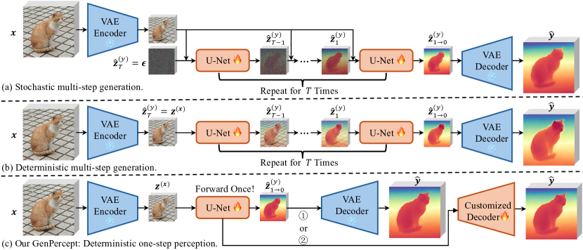
Figure 1: Comparisons of three different pipelines. Ours can not only infer in one step but also support customized decoders and loss functions. The VAE encoder’s original architecture is kept intact for our method, maintaining the encoding process’s consistency. However, we can use customized task-specific decoders by replacing the VAE decoder, which is designed and trained for image synthesis only.

2.1 Stochastic Multi-Step Generation

Standard diffusion models [63, 10, 70, 34] define a forward process to inject Gaussian noise $\bm{\epsilon}$ into the input data and a reverse denoising process to estimate noises and generate clean images with a denoiser $\bm{v}_{\theta}$. For latent diffusion models, the forward and reverse diffusion processes are performed in a latent space compressed by the encoder $\mathcal{E}$ and decoder $\mathcal{D}$ of variational autoencoder (VAE [40]).

While diffusion models generate images from noise, the visual perception tasks take RGB images as input. One approach to address the disparity is to reframe perception tasks as an RGB image-conditioned denoising diffusion generation process [39]. By doing so, we can seamlessly integrate the requirements of visual perception tasks with the capabilities of diffusion models, thereby leveraging the strengths of both paradigms.

For the training process, the RGB image $\mathbf{x}$ and ground-truth label $\mathbf{y}$ are encoded into the latent space with the VAE encoder $\mathbf{z}^{(\mathbf{x})}=\mathcal{E}(\mathbf{x})$, $\mathbf{z}^{(\mathbf{y})}=\mathcal{E}(\mathbf{y})$. The Gaussian noise $\bm{\epsilon}$ is added to the ground-truth label latent $\mathbf{z}^{(\mathbf{y})}$, and the noisy label latent $\mathbf{z}^{(\mathbf{y})}_{t}$ is concatenated with the clean image latent $\mathbf{z}^{(\mathbf{x})}$ as U-Net input $\mathbf{z}_{t}$ for each timestep:

$$\begin{gathered}\mathbf{z}^{(\mathbf{y})}_{t}=\sqrt{\bar{\alpha}_{t}}\mathbf{z}^{(\mathbf{y})}+\sqrt{1-\bar{\alpha}_{t}}\bm{\epsilon},~{}~{}t=[1,...,T],\\ \mathbf{z}_{t}=\text{concat}(\mathbf{z}^{(\mathbf{y})}_{t},\mathbf{z}^{(\mathbf{x})}),\end{gathered}$$ (1)

where $\bar{\alpha}_{t}=\prod_{s=1}^{t}{(1-\beta_{s})}$, and $\beta_{s}$ is sampled from a variance schedule $\{\beta_{t}\in(0,1)\}_{t=1}^{T}$. Then, the denoiser $\bm{v}_{\theta}(\cdot,\cdot)$ is enforced to learn the velocity of “v-prediction” [65] from a timestep $t$ and the corresponding input $\mathbf{z}_{t}$. During training, the parameters of VAE are frozen, and only the denoiser $\bm{v}_{\theta}$ is fine-tuned. The timestep is uniformly sampled from 1 to $T$.

$$\begin{gathered}\mathcal{L}=\mathbb{E}_{\mathbf{z}^{(\mathbf{y})},\bm{\epsilon}\sim\mathcal{N}(0,I),t\sim\mathcal{U}(T)}\left\|(\sqrt{\bar{\alpha}_{t}}\bm{\epsilon}-\sqrt{1-\bar{\alpha}_{t}}\mathbf{z}^{(\mathbf{y})})-\bm{v}_{\theta}(\mathbf{z}_{t},t)\right\|^{2}_{2}.\end{gathered}$$ (2)

For inference, a Gaussian noise $\bm{\epsilon}_{t}$ is randomly sampled and denoised step by step with the denoiser $\bm{v}_{\theta}(\cdot,\cdot)$.

$$\begin{gathered}\hat{\mathbf{z}}^{(\mathbf{y})}_{T}=\bm{\epsilon},~{}~{}\mathbf{z}_{t}=\text{concat}(\hat{\mathbf{z}}^{(\mathbf{y})}_{t},\mathbf{z}^{(\mathbf{x})}),~{}~{}t=[T,...,1],\\ \hat{\mathbf{z}}^{(\mathbf{y})}_{t\rightarrow 0}=\sqrt{\bar{\alpha}_{t}}\cdot\hat{\mathbf{z}}^{(\mathbf{y})}_{t}-\sqrt{1-\bar{\alpha}_{t}}\cdot\bm{v}_{\theta}(\mathbf{z}_{t},t),~{}~{}\hat{\bm{\bm{\epsilon}}}_{t}=\sqrt{\bar{\alpha}_{t}}\cdot\bm{v}_{\theta}(\mathbf{z}_{t},t)-\sqrt{1-\bar{\alpha}_{t}}\cdot\hat{\mathbf{z}}^{(\mathbf{y})}_{t},\\ \hat{\mathbf{z}}^{(\mathbf{y})}_{t-1}=\sqrt{\bar{\alpha}_{t-1}}\cdot\hat{\mathbf{z}}^{(\mathbf{y})}_{t\rightarrow 0}+\sqrt{1-\bar{\alpha}_{t-1}}\cdot\hat{\bm{\bm{\epsilon}}}_{t},~{}~{}\hat{\mathbf{y}}=\mathcal{D}(\hat{\mathbf{z}}^{(\mathbf{y})}_{1\rightarrow 0}).\end{gathered}$$ (3)

where the denoising process first computes the estimated noise $\hat{\bm{\bm{\epsilon}}}_{t}$ and the predicted clean latent code $\hat{\mathbf{z}}^{(\mathbf{y})}_{t\rightarrow 0}$ of timestep $t$ from the current latent code $\hat{\mathbf{z}}^{(\mathbf{y})}_{t}$ and the predicted velocity $\bm{v}_{\theta}(\mathbf{z}_{t},t)$. Then, it adds the computed noise $\hat{\bm{\bm{\epsilon}}}_{t}$ back to $\hat{\mathbf{z}}^{(\mathbf{y})}_{t\rightarrow 0}$ to get the latent code of timestep $t-1$. After repeating it for $T$ times, the predicted clean latent code $\hat{\mathbf{z}}^{(\mathbf{y})}_{1\rightarrow 0}$ is computed and sent to the VAE decoder $\mathcal{D}$ and estimate the target label $\hat{\mathbf{y}}$. During inference, $m$ randomly sampled noises are introduced to estimate $m$ different predictions, and they are averaged with an ensemble process to reduce the randomness of prediction and improve performance.

Weakness. The stochastic multi-step generation process performs well but faces two significant drawbacks. Firstly, its stochastic nature conflicts with the deterministic nature of perception tasks. Secondly, the high-computation ensemble strategy poses challenges across various perception tasks.

2.2 Deterministic Multi-Step Generation

The inherent random nature of diffusion models makes them challenging to apply to perceptual tasks, which typically aim for accurate results. As a result, existing works have replaced the original Gaussian noise with the target image as RGB noise [6, 43]. Technically, rather than introducing the random Gaussian noise $\bm{\epsilon}$ , we blend the ground-truth label latent $\mathbf{z}^{(\mathbf{y})}=\mathcal{E}(\mathbf{y})$ with the RGB image latent $\mathbf{z}^{(\mathbf{x})}=\mathcal{E}(\mathbf{x})$, which is formulated as:

$$\begin{gathered}\mathbf{z}_{t}=\mathbf{z}^{(\mathbf{y})}_{t}=\sqrt{\bar{\alpha}_{t}}\mathbf{z}^{(\mathbf{y})}+\sqrt{1-\bar{\alpha}_{t}}\mathbf{z}^{(\mathbf{x})},~{}~{}t=[1,...,T],\\ \end{gathered}$$ (4)

Furthermore, the input latent has been modified to the latent code of input image $\mathbf{z}^{(\mathbf{x})}$ instead of random Gaussian. Consequently, the learning objective function and the inference process are reformulated as follows.

$$\begin{gathered}\mathcal{L}=\mathbb{E}_{(\mathbf{z}^{(\mathbf{x})},\mathbf{z}^{(\mathbf{y})}),t\sim\mathcal{U}(T)}\left\|(\sqrt{\bar{\alpha}_{t}}\mathbf{z}^{(\mathbf{x})}-\sqrt{1-\bar{\alpha}_{t}}\mathbf{z}^{(\mathbf{y})})-\bm{v}_{\theta}(\mathbf{z}_{t},t)\right\|^{2}_{2}.\end{gathered}$$ (5)

$$\begin{gathered}\hat{\mathbf{z}}^{(\mathbf{y})}_{T}=\mathbf{z}^{(\mathbf{x})},~{}~{}t=[T,...,1],\\ \hat{\mathbf{z}}^{(\mathbf{y})}_{t\rightarrow 0}=\sqrt{\bar{\alpha}_{t}}\cdot\hat{\mathbf{z}}^{(\mathbf{y})}_{t}-\sqrt{1-\bar{\alpha}_{t}}\cdot\bm{v}_{\theta}(\hat{\mathbf{z}}^{(\mathbf{y})}_{t},t),\hat{\mathbf{z}}^{(\mathbf{x})}_{t}=\sqrt{\bar{\alpha}_{t}}\cdot\bm{v}_{\theta}(\hat{\mathbf{z}}^{(\mathbf{y})}_{t},t)-\sqrt{1-\bar{\alpha}_{t}}\cdot\hat{\mathbf{z}}^{(\mathbf{y})}_{t},\\ \hat{\mathbf{z}}^{(\mathbf{y})}_{t-1}=\sqrt{\bar{\alpha}_{t-1}}\cdot\hat{\mathbf{z}}^{(\mathbf{y})}_{t\rightarrow 0}+\sqrt{1-\bar{\alpha}_{t-1}}\cdot\hat{\mathbf{z}}^{(\mathbf{x})}_{t},~{}~{}\hat{\mathbf{y}}=\mathcal{D}(\hat{\mathbf{z}}^{(\mathbf{y})}_{1\rightarrow 0}).\end{gathered}$$ (6)

where $\hat{\mathbf{z}}^{(\mathbf{x})}_{t}$ denotes the predicted RGB noise of timestep $t$.

Weakness. The deterministic multi-step generation method effectively addresses the uncertainty inherent in the process. Nevertheless, when visualizing the estimated outcomes, the persistence of RGB texture in the generated perception predictions can detrimentally impact accuracy. This phenomenon is particularly evident in tasks such as surface normal estimation, as exemplified in Fig. 2.

2.3 Ours: Directly Using the Pre-trained UNet as Initialization

Analysis and Solution. To interpret this phenomenon, we suppose that blending with the RGB image is much simpler compared to a Gaussian noise. Therefore, we increase the blending proportion of the RGB image to make it more difficult. Practically, we realize it by increasing the initial value $\beta_{0}$ and final values $\beta_{T}$ of the variance schedule.

According to Fig. 2 and our ablation study, we find the results become better with the increase of RGB blending proportion. Therefore, we boldly try to purely input the RGB latent code, and it also works well. Mathematically, all the beta values $\{\beta_{t}\}_{t=1}^{T}$ are set to 1, and $\bar{\alpha}_{t}=\prod_{s=1}^{t}{(1-\beta_{s})}=0$, the formulation of Eq. 4 to Eq. 6 can be greatly simplified as follows.

$$\begin{gathered}\mathbf{z}_{t}=\mathbf{z}^{(\mathbf{y})}_{t}=\mathbf{z}^{(\mathbf{x})},~{}~{}\mathcal{L}=\mathbb{E}_{(\mathbf{z}^{(\mathbf{x})},\mathbf{z}^{(\mathbf{y})}),t\sim\mathcal{U}(T)}\left\|-\mathbf{z}^{(\mathbf{y})}-\bm{v}_{\theta}(\mathbf{z}_{t},t)\right\|^{2}_{2},\\ \hat{\mathbf{z}}^{(\mathbf{y})}_{T}=\mathbf{z}^{(\mathbf{x})},~{}~{}\hat{\mathbf{z}}^{(\mathbf{y})}_{t-1}=-\hat{\mathbf{z}}^{(\mathbf{y})}_{t},~{}~{}\hat{\mathbf{z}}^{(\mathbf{y})}_{1\rightarrow 0}=-\bm{v}_{\theta}(\hat{\mathbf{z}}^{(\mathbf{y})}_{1},t=1),~{}~{}\hat{\mathbf{y}}=\mathcal{D}(\hat{\mathbf{z}}^{(\mathbf{y})}_{1\rightarrow 0}).\end{gathered}$$ (7)

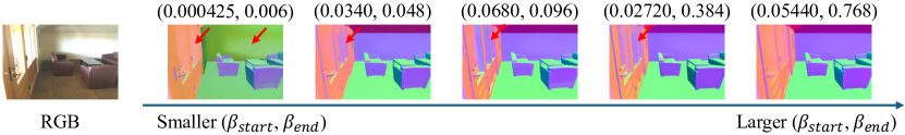
Figure 2: After increasing the blending proportion of the RGB image, the potential RGB information in the generated surface normal map becomes less.

Our Method. The input of the U-Net is an RGB latent code, and the output becomes the ground-truth latent code, with no relationship to the timestep $t$. Experimentally, we find that the number of timesteps $T$ will not affect the perception accuracy and therefore can be set to 1. Up to now, the quantitative changes have led to a change in quality, the stochastic multi-step generation has been transferred to the deterministic one-step perception, i.e., fine-tuning diffusion models as perception models within one step.

$$\begin{gathered}\mathcal{L}=\mathbb{E}_{(\mathbf{z}^{(\mathbf{x})},\mathbf{z}^{(\mathbf{y})})}\left\|-\mathbf{z}^{(\mathbf{y})}-\bm{v}_{\theta}(\mathbf{z}^{(\mathbf{x})},t=1)\right\|^{2}_{2},\\ \hat{\mathbf{z}}^{(\mathbf{y})}_{1\rightarrow 0}=-\bm{v}_{\theta}(\mathbf{z}^{(\mathbf{x})},t=1),~{}~{}\hat{\mathbf{y}}=\mathcal{D}(\hat{\mathbf{z}}^{(\mathbf{y})}_{1\rightarrow 0}).\end{gathered}$$ (8)

Note that this is simply to initialize the network using the pre-trained UNet and fine tune the model using labeled data.

Discussions. First, the training of the diffusion models is nothing more than training a denoising auto-encoder by adding multi-level noises to the latent VAE code. Thus, compared to self-supervised representation learning methods such as MAE [31], diffusion training follows the same overall idea of MAE; and they only differ in the subtle design of encoders and decoders and the types of noises used.

From the perspective of text-to-image (T2I) synthesis, T2I synthesis is likely to be effective for representation learning due to the following reasons: 1) Textual descriptions provide context and semantic information that can be used to guide the generation of images. 2) The ability to learn a mapping between text and images can lead to improved understanding and generation of both modalities. 3) The availability of large datasets, such as LAION, with paired text and image data, facilitates the training of T2I models.

Essentially, T2I is another form of supervision of text and image interaction. Recall that CLIP [57] associates text and images by applying a contrastive learning approach. This involves pushing apart incompatible text-image pairs and pulling closer compatible ones, adhering to conventional metric learning methodologies. According to CoCa of [86] on image captioning (I2T) for learning representations, the process leads to robust representations that can be effectively utilized for a wide range of downstream tasks with minimal adaptation or zero-shot transfer. Based on this observation, we anticipate that text-to-image (T2I) synthesis will also be capable of learning efficient image representations.

Customized Task-specific Decoder and Loss. Similar to traditional perception models, our GenPercept can leverage various customized perception decoders. The main advantages include: 1) Compared to the VAE decoder, the customized one can personalize the output channels, offering great flexibility. 2) Various losses can be used to further improve the performance. 3) The standard noise objective in Eq. 2 and Eq. 5 requires dense ground-truth labels to be encoded to latent space. However, for depth estimation, some ground-truth labels captured from sensors are sparse (LiDAR) or semi-dense (RGB-D cameras). The customized loss enables discarding the invalid regions and leveraging the valid ones.

3 Experiments

We empirically show the robust transfer ability of our GenPercept on diverse visual tasks. Then, ablation studies and analyses are shown in §3.5.

3.1 Geometric Estimation

Monocular Depth Estimation. The monocular depth estimation aims to predict the vertical distance between the observed object and the camera from an RGB image. The estimated depth is formulated as affine-invariant depth [84, 61, 60], and should be recovered by performing least square regression with the ground truth. The evaluation is performed on KITTI [29], NYU [69], DIODE [73], and ETH3D [66]. We compute the absolute relative error (AbsRel$\downarrow$) and percentage of accurate valid depth pixels ($\delta_{1}$$\uparrow$). Invalid regions are filtered out and the metrics are averaged on all images.

Table 1: Quantitative comparison of affine-invariant depth estimation.

Method	Synthetic	KITTI [29]		NYU [69]		DIODE [73]		ETH3D [66]
	Data Only?	AbsRel$\downarrow$	$\delta_{1}$$\uparrow$	AbsRel$\downarrow$	$\delta_{1}$$\uparrow$	AbsRel$\downarrow$	$\delta_{1}$$\uparrow$	AbsRel$\downarrow$	$\delta_{1}$$\uparrow$
DiverseDepth [83]	No	0.190	0.704	0.117	0.875	0.376	0.631	0.228	0.694
MiDaS [61]	No	0.236	0.630	0.111	0.885	0.332	0.715	0.184	0.752
LeReS [84]	No	0.149	0.784	0.090	0.916	0.271	0.766	0.171	0.777
Omnidata [21]	No	0.149	0.835	0.074	0.945	0.339	0.742	0.166	0.778
HDN [87]	No	0.115	0.867	0.069	0.948	0.246	0.780	0.121	0.833
DPT-large [60]	No	0.100	0.901	0.098	0.903	0.182	0.758	0.078	0.946
GenPercept	Yes	0.099	0.904	0.056	0.960	0.357	0.756	0.062	0.958

Table 2: Surface normal accuracy on NYUv2 [69] and ScanNet [16].

Method	Train Dataset	Test Dataset	Mean	Median	RMSE	$11.25^{\circ}$	$22.5^{\circ}$	$30^{\circ}$
FrameNet[38]	ScanNet [16]	NYU [69]	18.6	11.0	26.8	50.7	72.0	79.5
VPLNet[75]			18.0	9.8	-	54.3	73.8	80.7
TiltedSN[18]			16.1	8.1	25.1	59.8	77.4	83.4
Bae et al. [3]			16.0	8.4	24.7	59.0	77.5	83.7
GenPercept	Hypersim [62]	NYU [69]	16.9	9.2	26.5	58.3	79.0	84.7
Bae et al. [3]	NYU [69]	ScanNet [16]	23.1	14.0	33.114	43.3	65.5	73.6
GenPercept	Hypersim [62]	ScanNet [16]	18.6	9.7	29.5	55.8	76.6	82.6

Surface Normal Estimation. The surface normal estimation aims to predict a vector perpendicular to the tangent plane of the surface at each point P, which represents the orientation of the object’s surface. For evaluation, we follow Bae et al. [3] to compute the angular error on NYU [69] and ScanNet [16], whose ground-truth normal maps are provided by Ladicky et al. [42] and FrameNet [38]. The mean $\downarrow$, median $\downarrow$, root-mean-squared error (RMSE $\downarrow$), and the percentages of pixels $\uparrow$ with error below thresholds [11.25^∘, 22.5^∘, 30^∘] are reported. Invalid regions are filtered out and the metrics are averaged on all images.

Implementation Details. 1) The depth model is trained on Hypersim [62] and virtual KITTI [29]. We use the VAE encoder and U-Net of Stable Diffusion v2.1 and decode the feature with a DPT [60] decoder. Only the VAE encoder is frozen during training. The resolution is 768, the batch size is 16, and the learning rate is 3e-5 with linear decay. We use the VNL [82] loss, the HDN [87] loss, the MSE (mean squared error) loss, and the L1 loss as the customized loss. 2) The normal model is trained on Hypersim [62]. We use the original frozen VAE decoder and supervise MSE loss on the latent code space. The resolution, batch size, and learning rate are the same as those of depth estimation.

Quantitative Evaluation. Quantitative results on monocular depth estimation and surface normal estimation are shown in Table 1 and Tab. 2, respectively. Even trained on synthetic datasets only, we show much robustness and achieve promising performance on diverse unseen scenes.

Qualitative Results. Qualitative visualizations are shown in Fig. 3. We observe excellent generalization of our models in that they can estimate accurate geometric information not only on diverse real scenes and synthetic scenes, but also on comics, color drafts, and even some sketches that have a sense of depth.

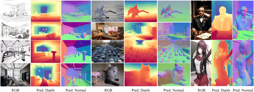
Figure 3: Qualitative results of monocular depth and surface normal estimation. Remarkably, the model works surprisingly well on out-of-domain images (sketch and cartoon images). Best viewed on screen.

3.2 Image Segmentation

Semantic Image Segmentation is a fundamental computer vision problem. We conducted ablation studies to assess the generation capability of our proposed architecture on the semantic segmentation task through cross-dataset evaluation. Our approach involves a two-stage pipeline. In the initial stage, we define semantic class labels using colormaps similar to [76], leveraging pre-training on latent space by supervising the output of UNet with color maps encoded by the VAE encoder using L2 loss. Subsequently, in the second stage, we incorporate a custom segmentation head, namely UperNet [80], onto the multi-level features extracted by UNet.

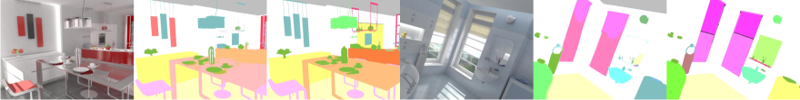
Figure 4: Visualization of the semantic segmentation output of the VAE decoder. Left: input image. Middle: VAE decoder output. Right: ground-truth colormaps.

For training, we utilized the indoor synthetic dataset, HyperSim [62], which comprises 40 semantic segmentation class labels. The evaluation was performed on a subset of the ADE20k dataset’s [93] validation set, which shares classes overlapping with HyperSim [62]. Table 3 showcases our model’s performance compared to DINOv2 [51] with ViT-Giant. Although our model exhibits lower inter-dataset performance compared to DINO-v2, it demonstrates similar intra-dataset generalization capacity. As shown in Fig. 4, we found the first stage pre-training on latent space can produce fine-grained masks by decoding the latent with the VAE decoder.

Table 3: Quantitative comparison of semantic segmentation on Hypersim [62] and ADE20k [93]. Both DINOv2 [51] and our model are trained on the Hypersim [62] dataset alone. FT: fine-tuning of backbone networks.

Method	Backbone	Params	Train. data	FT.	mIoU$\uparrow$ (Hypersim)	mIoU$\uparrow$ (ADE20K)
DINOv2 [51]	ViT-Giant	1100M	Hypersim		51.5	37.1
DINOv2 [51]	ViT-Giant	1100M	Hypersim	✓	58.6	41.2
Ours	U-Net	860M	Hypersim		46.0	34.1
Ours	U-Net	860M	Hypersim	✓	52.9	38.3

Dichotomous Image Segmentation. This is a category-agnostic, high-quality object segmentation task that accurately separates the object from the background in an image. Consistent with previous methods, we use the six evaluation metrics specified in the DIS task, which include maximal F-measure ($maxF_{\beta}\uparrow$) [1], weighted F-measure ($F^{w}_{\beta}\uparrow$) [47], mean absolute error ($~{}M\downarrow$) [52], structural measure ($S_{\alpha}\uparrow$) [24], mean enhanced alignment measure ($E_{\phi}^{m}\uparrow$) [25, 27] and human correction efforts (${\rm HCE}_{\gamma}\downarrow$) [54]. We choose DIS5K [54] as the training and testing dataset. We utilize DIS-TR for training and evaluate our model on DIS-VD and DIS-TE subsets. For training, we initialize the weights using Stable Diffusion v2.1 [63], and only fine-tune the U-Net while freezing the parameters of the remaining parts. The model is trained for 30,000 iterations with an initial learning rate of 3e$-5$ and a batch size of 32. We use the original VAE decoder to generate the output mask. In post-processing, we normalize predicted pixel values to $[0,1]$ using max-min normalization. Values below 0.5 are set to 0; and others are set to 1.

Table 4: Quantitative results of dichotomous image segmentation on DIS5K validation and testing sets. Additional cross-dataset evaluation is provided in the supplementary material.

Dataset	DIS-VD						DIS-TE4						Overall DIS-TE (1-4)
Metric	$maxF_{\beta}\uparrow$	$F^{w}_{\beta}\uparrow$	$~{}M\downarrow$	$S_{\alpha}\uparrow$	$E_{\phi}^{m}\uparrow$	${\rm HCE}_{\gamma}\downarrow$	$maxF_{\beta}\uparrow$	$F^{w}_{\beta}\uparrow$	$~{}M\downarrow$	$S_{\alpha}\uparrow$	$E_{\phi}^{m}\uparrow$	${\rm HCE}_{\gamma}\downarrow$	$maxF_{\beta}\uparrow$	$F^{w}_{\beta}\uparrow$	$~{}M\downarrow$	$S_{\alpha}\uparrow$	$E_{\phi}^{m}\uparrow$	${\rm HCE}_{\gamma}\downarrow$
U2Net[55]	0.748	0.656	0.090	0.781	0.823	1413	0.795	0.705	0.087	0.807	0.847	3653	0.761	0.670	0.083	0.791	0.835	1333
SINetV2[26]	0.665	0.584	0.110	0.727	0.798	1568	0.699	0.616	0.113	0.744	0.824	3683	0.693	0.608	0.101	0.747	0.822	1411
HySM[49]	0.734	0.640	0.096	0.773	0.814	1324	0.782	0.693	0.091	0.802	0.842	3331	0.757	0.665	0.084	0.792	0.834	1218
IS-Net[54]	0.791	0.717	0.074	0.813	0.856	1116	0.827	0.753	0.072	0.830	0.870	2888	0.799	0.726	0.070	0.819	0.858	1016
Ours	0.844	0.824	0.044	0.863	0.924	1495	0.841	0.823	0.049	0.849	0.934	3719	0.840	0.817	0.044	0.860	0.920	1333

Quantitative Evaluation. To conduct a comprehensive evaluation, we compare our approach with some previous models [55, 26, 49] and the model IS-Net [54] specifically trained for DIS. Due to length limitations, we only show partial results in Table 4, with complete results available in the Sup. Mat. Our proposed model outperforms all other methods by a significant margin on this challenging dataset across most evaluation metrics. The results highlight the effectiveness of our approach for DIS. Compared to previous methods, the segmentation results of our approach are more refined, providing a more detailed foreground mask. For thin lines and meticulous objects that are difficult for previous methods to process, our method can also output accurate segmentation results. The qualitative comparisons of our model and other models are shown in Fig. 5.

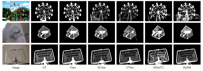
Figure 5: Qualitative comparison of dichotomous image segmentation.

3.3 Image Matting

Image Matting aims to predict the foreground, background, and alpha mask from a single input image. Therefore, an auxiliary input like the trimap, which divides the image into three types of areas: foreground, background, and unknown regions, is often required to mitigate the uncertainty. Recently, automatic image matting has been developed to eliminate the dependence on auxiliary inputs. We show that our paradigm is capable of predicting alpha masks from a single image without any additional auxiliary inputs.

Datasets We use P3M10K [44], the largest portrait matting dataset with high-resolution portrait images along with high-quality alpha masks. We train our model with 9,421 images in the training set, and evaluate the prediction result using P3M-500-NP which including 500 public celebrity images from the Internet without face obfuscation.

Implementation Details. For training, we initialize the weights using Stable Diffusion v2.1 [63], and only fine-tune the U-Net while freezing the parameters of the remaining parts. The model uses the DDPM scheduler [34] with 1,000 steps, training for 20,000 iterations with an initial learning rate of 3e-5 and a batch size of 32. For inference, the model uses the DDIM scheduler [70] with 51 steps. For post-processing, we scale the predicted pixel values to $[0,1]$ using max-min, we empirically set values greater than 0.95 to 1, and values less than 0.1 to 0.

Evaluation. As shown in Table 6, our pipeline is comparable with the state-of-the-art method, P3M [44] on the P3M-500-NP test set. We use the evaluation metrics including the sum of absolute differences (SAD), mean squared error (MSE), mean absolute difference (MAD), gradient (Grad.), and Connectivity (Conn.). We showcase our Image matting estimation results in Fig. 6.

Table 5: Image Matting on P3M-500-NP.

Method	SAD $\downarrow$	MAD $\downarrow$	MSE $\downarrow$	CONN $\downarrow$
P3M[44]	11.23	0.0065	0.0035	12.51
GenPercept	12.44	0.0071	0.0037	11.77

Table 6: Pose estimation on COCO.

Metrics	AP $\uparrow$	AP .5 $\uparrow$	AP .75 $\uparrow$	AP (M) $\uparrow$	AP (L) $\uparrow$
Painter[76]	0.721	0.900	0.781	0.686	0.786
GenPercept	0.752	0.907	0.824	0.691	0.778

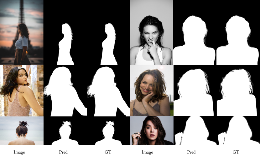
Figure 6: Visualization of image matting on the P3M-500-NP test set.

Figure 7: Generalized test results of keypoint detection.

3.4 Human Pose Estimation

Task Definition Human Pose Estimation is a task aimed at determining the spatial configuration of a person or object in a given image or video. This involves identifying and predicting the coordinates of particular keypoints.

Implementation Details For human keypoint detection, we use Simple Baseline[79] for person detection, and perform training on the COCO training set with 15K training samples. Performance is evaluated on the COCO [46] validation set. As shown in Fig. 7, our method is generalizable to unseen objects in the training set. To evaluate the performance on COCO, we use the keypoint head of ViTPose [81] for decoding the output. The quantitative results compared with a generalist model, Painter[76] is shown in Table 6.

3.5 Ablation Study

In this subsection, we perform detailed ablation studies and concentrate on the robustness and key components of our GenPercept.

Implementation Details. By default, experiments in this subsection are trained on the Hypersim dataset to estimate monocular depth. The Stable Diffusion v2.1 model is leveraged to provide prior knowledge of perception. We take an RGB image as input, freeze the VAE AutoEncoder, and fine-tune the U-Net to estimate the ground-truth label latent, with a resolution of 768, a batch size of 16, and a learning rate of 3e-5 with linear decay.

Multi-Step Generation vs. One-Step Perception. Following the development process of our GenPercept in §2, we perform quantitative comparisons of different ways to leverage diffusion model priors in Table 7. “Stochastic Multi-Step Generation” in §2.1 brings randomness to the perception tasks and can be time-consuming for the ensemble process. “Deterministic Multi-Step Generation” in §2.2 replaces the random noise with the RGB latent to remove the uncertainty, but it suffers from the residue of RGB information for the prediction. In Table 8, we find that it can be alleviated by increasing the proportion of RGB images during blending. Different from previous paradigms, our GenPercept introduced in §2.3 reformulates it as a perception task, and can not only save around $70\%$ inference time but also significantly improve the performance.

Table 7: Comparisons of different paradigms to leverage diffusion model priors. MS: multi-step diffusion. OS: one-step inference.

Setting	Inference	GPU	KITTI [29]		NYU [69]		DIODE [73]		ETH3D [66]
	Time (Sec.)	Memory	AbsRel$\downarrow$	$\delta_{1}$$\uparrow$	AbsRel$\downarrow$	$\delta_{1}$$\uparrow$	AbsRel$\downarrow$	$\delta_{1}$$\uparrow$	AbsRel$\downarrow$	$\delta_{1}$$\uparrow$
Stochastic MS Gen. (w. ensemble)	10$\times$10 ($\sim$20s)	42GB	0.185	0.719	0.078	0.929	0.424	0.730	0.075	0.942
Stochastic MS Gen. (w/o ensemble)	1$\times$10 ($\sim$1.25s)	9.7GB	0.191	0.698	0.078	0.929	0.416	0.727	0.076	0.939
Deterministic MS Gen.	1$\times$10 ($\sim$1.25s)	9.7GB	0.310	0.528	Failed		Failed		0.094	0.913
Deterministic OS infer.  (Ours)	1$\times$1 ($\sim$0.4s)	9.7GB	0.140	0.809	0.059	0.958	0.373	0.749	0.066	0.955

Table 8: Comparisons of different $\beta$ values in the “Deterministic Multi-Step Generation” paradigm. “($\beta_{start}$, $\beta_{end}$)” means the start and end values of $\beta$ curve in DDIM [70] scheduler. A larger $\beta$ value brings a larger proportion of RGB images during blending.

($\beta_{start}$, $\beta_{end}$)	KITTI [29]		NYU [69]		DIODE [73]		ETH3D [66]
	AbsRel$\downarrow$	$\delta_{1}$$\uparrow$	AbsRel$\downarrow$	$\delta_{1}$$\uparrow$	AbsRel$\downarrow$	$\delta_{1}$$\uparrow$	AbsRel$\downarrow$	$\delta_{1}$$\uparrow$
(0.00085, 0.012)	0.310	0.528	Failed		Failed		0.094	0.913
(0.00340, 0.048)	0.190	0.702	0.078	0.935	0.475	0.738	0.073	0.942
(0.1360, 0.192)	0.168	0.751	0.068	0.949	0.420	0.746	0.069	0.951
(0.5440, 0.768)	0.142	0.811	0.064	0.954	0.415	0.748	0.069	0.952

Table 9: Analysis for key components of GenPercept on affine-invariant monocular depth estimation.

Setting	KITTI [29]		NYU [69]		DIODE [73]		ETH3D [66]
	AbsRel$\downarrow$	$\delta_{1}$$\uparrow$	AbsRel$\downarrow$	$\delta_{1}$$\uparrow$	AbsRel$\downarrow$	$\delta_{1}$$\uparrow$	AbsRel$\downarrow$	$\delta_{1}$$\uparrow$
Baseline	0.140	0.809	0.059	0.958	0.373	0.749	0.066	0.955
Train U-Net from scratch	0.326	0.517	0.162	0.782	0.474	0.628	0.170	0.791
Fine-tune U-Net + DPT [60] decoder	0.166	0.747	0.058	0.960	0.351	0.745	0.074	0.941
Customized VAE encoder + Fine-tune U-Net	0.205	0.671	0.073	0.940	0.439	0.713	0.093	0.917
Freeze U-Net + Fine-tune DPT [60] decoder	0.330	0.442	0.104	0.899	0.423	0.655	0.164	0.784

Key Components Analysis. In Table 9, we explore the key components of Stable Diffusion v2.1 by replacing them one by one with other candidates.

1) We reinitialize the U-Net parameter and train it on Hypersim for 200K iterations. Without prior knowledge of large data from LAION-5B, the network performs poorly and loses the generalization. It shows the importance of large pre-train data for the U-Net.

2) We replace the pre-trained VAE decoder with the DPT decoder initialized from scratch. After fine-tuning for 30K iterations, it performs comparable to the baseline result, indicating that the parameter and architecture of the latent code decoder are not so significant.

3) To explore the importance of the VAE encoder, we simply train a VAE AutoEncoder on the Hypersim dataset only, freeze the trained VAE encoder, and finetune the U-Net as the previous experiments did. Without the pre-trained VAE decoder, the fine-tuned model is less accurate, but it still shows quite robust generalization on diverse datasets.

4) Simply freezing the U-Net, regarding it as an image feature extractor, and training a decoder on synthetic data is not a good choice. After freezing the U-Net, although a DPT decoder is trained on the Hypersim dataset, the performance is still poor. A possible reason is that the origin Stable Diffusion takes the blending of noise and RGB latent as input, and therefore can not perfectly handle the pure RGB latent input for perception tasks.

Table 10: Ablation study of the U-Net architecture on affine-invariant monocular depth estimation.

Setting	KITTI [29]		NYU [69]		DIODE [73]		ETH3D [66]
	AbsRel$\downarrow$	$\delta_{1}$$\uparrow$	AbsRel$\downarrow$	$\delta_{1}$$\uparrow$	AbsRel$\downarrow$	$\delta_{1}$$\uparrow$	AbsRel$\downarrow$	$\delta_{1}$$\uparrow$
GenPercent (SDv2.1 [63])	0.145	0.799	0.060	0.956	0.380	0.744	0.070	0.949
GenPercent (PixArt-$\alpha$ [10])	0.213	0.648	0.082	0.924	0.398	0.737	0.073	0.951

Robustness. The proposed one-step perception paradigm is not limited to the convolutional architecture of U-Net. As shown in Table 10, we replace the U-Net with transformer-based architecture PixArt-$\alpha$ [10]. With the strong transformer network, it can also generalize well to diverse test datasets. However, the PixArt-$\alpha$ model is trained on 25 million data (around 1% of Stable Diffusion v2.1), therefore it achieves less accurate performance.

Table 11: Comparison to DINOv2 [51] pre-training on affine-invariant monocular depth estimation.

Setting	KITTI [29]		NYU [69]		DIODE [73]		ETH3D [66]
	AbsRel$\downarrow$	$\delta_{1}$$\uparrow$	AbsRel$\downarrow$	$\delta_{1}$$\uparrow$	AbsRel$\downarrow$	$\delta_{1}$$\uparrow$	AbsRel$\downarrow$	$\delta_{1}$$\uparrow$
Genpercept + DPT [60] decoder	0.166	0.747	0.058	0.960	0.351	0.745	0.074	0.941
DINOv2 [51] + DPT [60] decoder	0.185	0.696	0.050	0.969	0.340	0.761	0.067	0.953

Comparison to Traditional Pre-trained Backbones. Comparisons to the strong DINOv2 [51] backbone are shown in Table 11. We adopt the U-Net of Stable Diffusion v2.1 (SD v2.1) and “dinov2-giant” strong backbone of DINOV2, followed with a DPT decoder and fine-tune them separately. With more parameters, the DINOv2 performs slightly better than SD v2.1, but worse performance on KITTI. We consider it as the strong generalization of SD v2.1, because it can generalize well to outdoor scenes although only trained on the Hypersim indoor dataset.

Table 12: Ablation study on the amount of training data on affine-invariant monocular depth estimation.

Amount of Data	KITTI [29]		NYU [69]		DIODE [73]		ETH3D [66]
	AbsRel$\downarrow$	$\delta_{1}$$\uparrow$	AbsRel$\downarrow$	$\delta_{1}$$\uparrow$	AbsRel$\downarrow$	$\delta_{1}$$\uparrow$	AbsRel$\downarrow$	$\delta_{1}$$\uparrow$
44K (1/1)	0.140	0.809	0.059	0.958	0.373	0.749	0.066	0.955
22K (1/2)	0.161	0.754	0.060	0.959	0.342	0.745	0.069	0.949
11K (1/4)	0.175	0.720	0.064	0.953	0.370	0.728	0.076	0.940
5.5K (1/8)	0.192	0.672	0.067	0.951	0.355	0.729	0.079	0.934
2.7K (1/16)	0.225	0.592	0.071	0.946	0.371	0.713	0.099	0.898
1.4K (1/32)	0.259	0.525	0.077	0.934	0.369	0.699	0.114	0.874
0.6K (1/64)	0.295	0.479	0.086	0.923	0.371	0.694	0.132	0.839
0.3K (1/128)	0.335	0.422	0.106	0.890	0.368	0.681	0.150	0.805

Requirements for Finetuning Data. With only around 44K synthetic data (Hypersim [62]) for fine-tuning, GenPercept can generalize well to diverse tasks and datasets. How much data is needed for transferring at least? We gradually reduce the amount of training data. As shown in Table 12, less training data results in worse performance. But it’s surprising that even trained with 300 images, the quantitative performance and visualization are still not bad.

4 Related work

Diffusion Models. Diffusion probability models and related training and sampling methods, such as Denoising Diffusion Probability Models[34], Denoising Diffusion Implicit Models[70], and score-based diffusion[70], have laid the foundation for recent advancements in large-scale image generation. In the domain of text-based image generation, Rombach et al. trained a latent diffusion model called Stable Diffusion[63] on a large-scale image and text dataset, LAION-5B, and demonstrated previously unachievable image synthesis quality. In contrast to Stable Diffusion, DeepFloyd IF operates directly in the pixel space. PixArt[10] utilizes Diffusion Transformer as the underlying architecture for handling text-to-image tasks. These models extract internet-scale image collections as model weights, thereby developing a rich prior understanding of scenes.

Transferring Pre-Trained Models. Models pretrained on large-scale datasets possess powerful feature extraction capabilities, enabling them to be effectively transferred to a wide range of visual tasks. For instance, the ResNet[33] model pretrained on ImageNet can be fine-tuned and applied to perception tasks. By means of contrastive learning, MoCo[32] and CLIP[57] acquire rich visual and semantic representations, leveraging their advantages in joint visual and semantic modeling to enhance the performance of multimodal tasks. DINO[88], through self-distillation, endows Vision Transformer and convolutional networks with comparable visual representation quality and demonstrates that self-supervised ViT representations contain explicit semantic segmentation information. In our work, we leverage Stable Diffusion[63] as a prior for scene understanding and transfer it to various perception tasks.

Perceptual Prior of Generative Models. Several works explore to use the priors of generative models for perceptual tasks. Some works [8, 20] demonstrate that generative models encode property maps of the scene. By finding latent variable offsets, using LoRA [37], etc., generative models can directly produce intrinsic images like surface normals, depth, albedo, etc. LDMSeg [72] devises an image-conditioned sampling process, enabling diffusion models to directly output panoptic segmentation. UniGS [53] proposes location-aware color encoding and decoding strategies, allowing diffusion models to support referring segmentation and entity segmentation. Marigold [39] fine-tunes diffusion model on limited synthetic data, enabling it to support affine-invariant monocular depth estimation and exhibit strong generalization performance. However, Marigold is time-consuming due to the need for multiple iterations of denoising. Additionally, the Gaussian noise leads to inconsistent results across inferences, requiring aggregation over multiple inferences. Xiang et al. [78] train a denoising auto-encoder for image classification. The difference of their method compared with traditional denoising auto-encoder is that input images are encoded into a latent code and denoising is performed in the latent space rather than the pixel space. They show good results on very small-scale datasets (CIFAR and ImageNet-tiny) to prove the concept and no results were reported on larger datasets.

5 Conclusion

In this work, We have introduced GenPercept, an embarrassingly straightforward yet powerful approach to re-use the off-the-shelf UNet trained using diffusion processes. In essence, we initialize our image perception networks using pre-trained U-Net or transformer models trained on the extensive LAION dataset, without making many modifications. GenPercept demonstrates the capability to effectively leverage pre-trained diffusion models across a range of downstream perception tasks. We contend that our proposed methodology provides an efficient and potent paradigm for harnessing the capabilities of pre-trained diffusion models in vision perception tasks.

Appendix 0.A More Analysis Experiments

Comparison to Traditional Pre-trained Backbones. Comparisons to the CLIP [57] vision model is shown in Table 13 and Fig. 8. We adopt the U-Net of Stable Diffusion v2.1 [63] (SD v2.1) and the “CLIP-ViT-bigG-14” strong CLIP model followed by a DPT [60] decoder. Both the adopted network and the decoder are fine-tuned during training. Our GenPercept can not only achieve better performance but also estimate the perception details from RGB images. For the CLIP model experiment, we set the learning rates of the CLIP model and the DPT decoder to 3e-6 and 1e-4, respectively. Other settings are the same as the ablation study in the main paper.

Table 13: Comparison to CLIP [57] pre-training on affine-invariant monocular depth estimation.

Setting	KITTI [29]		NYU [69]		DIODE [73]		ETH3D [66]
	AbsRel$\downarrow$	$\delta_{1}$$\uparrow$	AbsRel$\downarrow$	$\delta_{1}$$\uparrow$	AbsRel$\downarrow$	$\delta_{1}$$\uparrow$	AbsRel$\downarrow$	$\delta_{1}$$\uparrow$
GenPercept + DPT [60] decoder	0.166	0.747	0.058	0.960	0.351	0.745	0.074	0.941
CLIP [57] + DPT [60] decoder	0.227	0.607	0.080	0.936	0.360	0.718	0.106	0.901

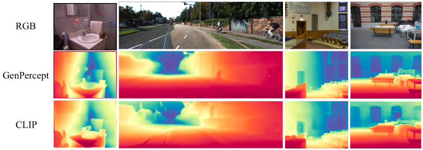
Figure 8: Qualitative comparisons of two different pre-trained backbones: U-Net of Stable Diffusion v2.1 [63] and “ViT-bigG-14” of CLIP [57].

Apart from fine-tuning. We compare the fine-tuning training paradigm to LoRA [37] and ControlNet [89] in Table 14 and Fig. 9. Both LoRA and ControlNet can hardly predict accurate details of monocular depth. The learning rates of LoRA and ControlNet are set to 1e$-4$ and 3e$-5$.

Table 14: Besides fine-tuning, we also adopt the training paradigm of LoRA [37] and ControlNet [89] to adapt U-Net to perception tasks.

Setting	KITTI [29]		NYU [69]		DIODE [73]		ETH3D [66]
	AbsRel$\downarrow$	$\delta_{1}$$\uparrow$	AbsRel$\downarrow$	$\delta_{1}$$\uparrow$	AbsRel$\downarrow$	$\delta_{1}$$\uparrow$	AbsRel$\downarrow$	$\delta_{1}$$\uparrow$
Fine-tuning	0.140	0.809	0.059	0.958	0.373	0.749	0.066	0.955
LoRA [37]	0.295	0.473	0.086	0.929	0.388	0.710	0.106	0.891
ControlNet [89]	0.248	0.567	0.124	0.855	0.386	0.708	0.112	0.877

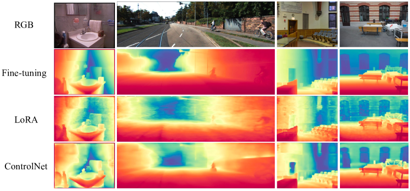
Figure 9: Qualitative comparisons of three different training paradigms: fine-tuning, LoRA [37], and ControlNet [89].

Appendix 0.B More Detailed Experiments

0.B.1 Monocular Depth Estimation

Affine-invariant Depth. Given an RGB image, the monocular depth estimation aims to recover the 3D geometry structure by predicting the vertical distance between the observed object and the camera. The estimated depth is usually formulated as affine-invariant depth [84, 61, 60], i.e., the transformation between the ground-truth depth and the predicted depth is an unknown affine transformation. Usually, the scale and shift of affine transformation can be recovered by performing least square regression [84, 61, 60] with the ground truth.

Datasets. KITTI [29] and NYU [69] are captured by LIDAR on outdoor streets and Kinect in indoor rooms, whose test splits contain 652 and 654 images, respectively. DIODE [73] includes 771 high-resolution RGB-D pairs of both indoor and outdoor scenes. The test split of ETH3D [66] covers 454 images and their ground-truth geometry was obtained with a high-precision laser scanner. For ETH3D, we resize the high-resolution images to $504\times 756$. For KITTI, “kb_crop” is performed. For KITTI and NYU, we follow Eigen et al. [22] to filter out invalid regions of image edges. For DIODE, the official invalid regions are used to filter out ground-truth depth. For ETH3D, we resize the high-resolution images to (504, 756) for fast evaluation. Note that the ground-truth depth maps for outdoor scenes of DIODE are noisy, therefore the performance of DIODE will not be exact.

Implementation Details. For the Hypersim dataset, we filter out the invalid RGB images and depth maps, which contain “NaN (not a number)”, “infinitive”, and “all-zero” values. The ground truth of Hypersim is actually the distance from a point to the camera, and it is converted to the vertical distance to the camera plane (i.e., depth values). The prompts of the text encoder are fixed to empty. During training, the extreme depth values that are larger than 98% or smaller than 2% are clipped before normalization. For Virtual KITTI, depth values larger than 500m are filtered out before clipping. The shortest edge of images is resized to 768 while keeping the aspect ratio. Then, a center crop of (768, 768) is performed, and the images are normalized to (-1, 1) before passing through the pre-trained VAE encoder. The timestep input of U-Net is set to 1 for our one-step GenPerception. The last ReLU [30] activation function of the DPT decoder is replaced by ELU [14] plus 1, i.e., $y=ELU(x)+1$.

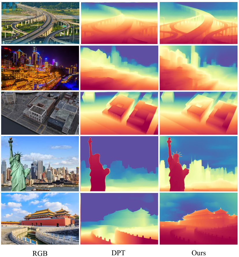
Figure 12: More qualitative results for monocular depth estimation.

More Qualitative Evaluation. We show the robustness of the monocular depth estimation model in diverse scenes in Fig. 12. Compared to DPT [60], our Genpercept performs better on estimating details and shows much better robustness even on some sketches.

0.B.2 Surface Normal Estimation

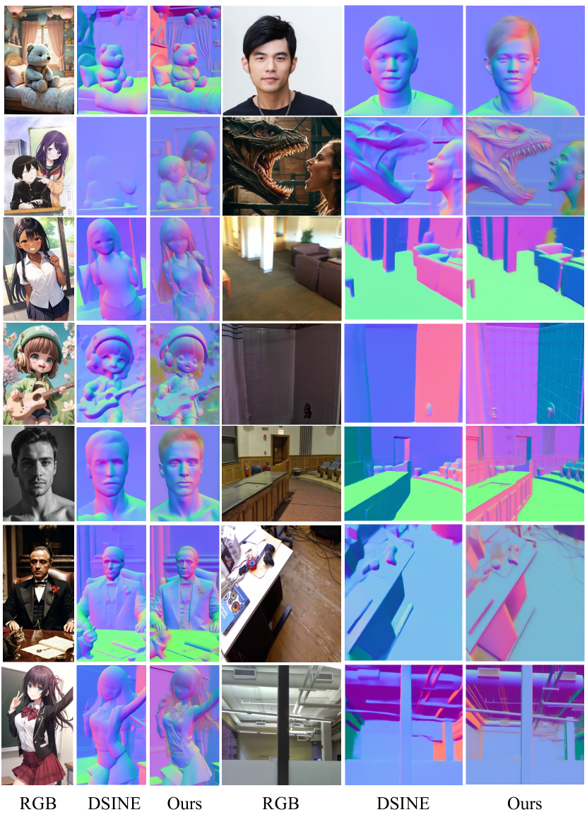
Figure 13: More qualitative comparisons of surface normal estimation. Our GenPercept can achieve more detailed results, even compared to the competitive CVPR’24 method DSINE [4]. Note that these two visualization coordinate systems are slightly different.

More Qualitative Evaluation. In Fig. 13, we showcase more qualitative results for the surface normal estimation. DSINE [4] is trained on 160K images of 10 datasets, including both real and synthetic data. Our GenPercept is only trained on one synthetic dataset (Hypersim [62]), and can estimate much more detailed surface normal maps.

0.B.3 Dichotomous Image Segmentation

Dichotomous Image Segmentation. This is a category-agnostic, high-quality object segmentation task that accurately separates the object from the background in an image. In comparison to previous segmentation tasks, DIS demands higher segmentation accuracy while disregarding the category and characteristics of the segmented objects. Due to its superior segmentation results, DIS can be applied in various domains, such as image editing, 3D reconstruction, medical image processing, etc.

Datasets. We choose DIS5K [54] as the training and testing dataset. DIS5K comprises 5,470 images of high resolutions with corresponding high-quality segmentation annotations and encompasses challenging segmentation scenarios, such as camouflaged objects or intricate objects with cavities. It is divided into three subsets: DIS-TR (3,000), DIS-VD (470) and DIS-TE (2,000) for training, validation and testing. Specifically, DIS-TE is further subdivided into four subsets (DIS-TE1 to DIS-TE4) based on structure complexities and boundary complexities, ranging from easy to difficult, each containing 500 images.

More Quantitative Evaluation. To conduct a comprehensive evaluation, we compare our approach with numerous previous models including models for medical image segmentation [64], salient object detection [56, 92, 77, 12, 55], camouflaged object detection [26, 48], semantic segmentation [91, 11, 74, 85, 90, 36, 28, 49] and the model IS-Net [54] specifically trained for DIS. As shown in Table 15, our proposed model significantly outperforms other methods across most evaluation metrics on this challenging dataset. The results highlight the effectiveness of our approach for DIS.

Table 15: Quantitative results on DIS5K validation and testing sets.

Dataset	Metric	UNet [64]	BASNet [56]	GateNet [92]	F3Net [77]	GCPANet [12]	U2Net [55]	SINetV2 [26]	PFNet [48]	PSPNet [91]	DLV3+ [11]	HRNet [74]	BSV1 [85]	ICNet [90]	MBV3 [36]	STDC [28]	HySM [49]	IS-Net [54]	Ours
DIS-VD	$maxF_{\beta}\uparrow$	0.692	0.731	0.678	0.685	0.648	0.748	0.665	0.691	0.691	0.660	0.726	0.662	0.697	0.714	0.696	0.734	0.791	0.844
	$F^{w}_{\beta}\uparrow$	0.586	0.641	0.574	0.595	0.542	0.656	0.584	0.604	0.603	0.568	0.641	0.548	0.609	0.642	0.613	0.640	0.717	0.824
	$~{}M~{}\downarrow$	0.113	0.094	0.110	0.107	0.118	0.090	0.110	0.106	0.102	0.114	0.095	0.116	0.102	0.092	0.103	0.096	0.074	0.044
	$S_{\alpha}\uparrow$	0.745	0.768	0.723	0.733	0.718	0.781	0.727	0.740	0.744	0.716	0.767	0.728	0.747	0.758	0.740	0.773	0.813	0.863
	$E_{\phi}^{m}\uparrow$	0.785	0.816	0.783	0.800	0.765	0.823	0.798	0.811	0.802	0.796	0.824	0.767	0.811	0.841	0.817	0.814	0.856	0.924
	${\rm HCE}_{\gamma}\downarrow$	1337	1402	1493	1567	1555	1413	1568	1606	1588	1520	1560	1660	1503	1625	1598	1324	1116	1495
DIS-TE1	$maxF_{\beta}\uparrow$	0.625	0.688	0.620	0.640	0.598	0.694	0.644	0.646	0.645	0.601	0.668	0.595	0.631	0.669	0.648	0.695	0.740	0.807
	$F^{w}_{\beta}\uparrow$	0.514	0.595	0.517	0.549	0.495	0.601	0.558	0.552	0.557	0.506	0.579	0.474	0.535	0.595	0.562	0.597	0.662	0.781
	$~{}M~{}\downarrow$	0.106	0.084	0.099	0.095	0.103	0.083	0.094	0.094	0.089	0.102	0.088	0.108	0.095	0.083	0.090	0.082	0.074	0.043
	$S_{\alpha}\uparrow$	0.716	0.754	0.701	0.721	0.705	0.760	0.727	0.722	0.725	0.694	0.742	0.695	0.716	0.740	0.723	0.761	0.787	0.852
	$E_{\phi}^{m}\uparrow$	0.750	0.801	0.766	0.783	0.750	0.801	0.791	0.786	0.791	0.772	0.797	0.741	0.784	0.818	0.798	0.803	0.820	0.889
	${\rm HCE}_{\gamma}\downarrow$	233	220	230	244	271	224	274	253	267	234	262	288	234	274	249	205	149	198
DIS-TE2	$maxF_{\beta}\uparrow$	0.703	0.755	0.702	0.712	0.673	0.756	0.700	0.720	0.724	0.681	0.747	0.680	0.716	0.743	0.720	0.759	0.799	0.849
	$F^{w}_{\beta}\uparrow$	0.597	0.668	0.598	0.620	0.570	0.668	0.618	0.633	0.636	0.587	0.664	0.564	0.627	0.672	0.636	0.667	0.728	0.827
	$~{}M~{}\downarrow$	0.107	0.084	0.102	0.097	0.109	0.085	0.099	0.096	0.092	0.105	0.087	0.111	0.095	0.083	0.092	0.085	0.070	0.042
	$S_{\alpha}\uparrow$	0.755	0.786	0.737	0.755	0.735	0.788	0.753	0.761	0.763	0.729	0.784	0.740	0.759	0.777	0.759	0.794	0.823	0.869
	$E_{\phi}^{m}\uparrow$	0.796	0.836	0.804	0.820	0.786	0.833	0.823	0.829	0.828	0.813	0.840	0.781	0.826	0.856	0.834	0.832	0.858	0.922
	${\rm HCE}_{\gamma}\downarrow$	474	480	501	542	574	490	593	567	586	516	555	621	512	600	556	451	340	460
DIS-TE3	$maxF_{\beta}\uparrow$	0.748	0.785	0.726	0.743	0.699	0.798	0.730	0.751	0.747	0.717	0.784	0.710	0.752	0.772	0.745	0.792	0.830	0.862
	$F^{w}_{\beta}\uparrow$	0.644	0.696	0.620	0.656	0.590	0.707	0.641	0.664	0.657	0.623	0.700	0.595	0.664	0.702	0.662	0.701	0.758	0.839
	$~{}M~{}\downarrow$	0.098	0.083	0.103	0.092	0.109	0.079	0.096	0.092	0.092	0.102	0.080	0.109	0.091	0.078	0.090	0.079	0.064	0.042
	$S_{\alpha}\uparrow$	0.780	0.798	0.747	0.773	0.748	0.809	0.766	0.777	0.774	0.749	0.805	0.757	0.780	0.794	0.771	0.811	0.836	0.869
	$E_{\phi}^{m}\uparrow$	0.827	0.856	0.815	0.848	0.801	0.858	0.849	0.854	0.843	0.833	0.869	0.801	0.852	0.880	0.855	0.857	0.883	0.935
	${\rm HCE}_{\gamma}\downarrow$	883	948	972	1059	1058	965	1096	1082	1111	999	1049	1146	1001	1136	1081	887	687	956
DIS-TE4	$maxF_{\beta}\uparrow$	0.759	0.780	0.729	0.721	0.670	0.795	0.699	0.731	0.725	0.715	0.772	0.710	0.749	0.736	0.731	0.782	0.827	0.841
	$F^{w}_{\beta}\uparrow$	0.659	0.693	0.625	0.633	0.559	0.705	0.616	0.647	0.630	0.621	0.687	0.598	0.663	0.664	0.652	0.693	0.753	0.823
	$~{}M~{}\downarrow$	0.102	0.091	0.109	0.107	0.127	0.087	0.113	0.107	0.107	0.111	0.092	0.114	0.099	0.098	0.102	0.091	0.072	0.049
	$S_{\alpha}\uparrow$	0.784	0.794	0.743	0.752	0.723	0.807	0.744	0.763	0.758	0.744	0.792	0.755	0.776	0.770	0.762	0.802	0.830	0.849
	$E_{\phi}^{m}\uparrow$	0.821	0.848	0.803	0.825	0.767	0.847	0.824	0.838	0.815	0.820	0.854	0.788	0.837	0.848	0.841	0.842	0.870	0.934
	${\rm HCE}_{\gamma}\downarrow$	3218	3601	3654	3760	3678	3653	3683	3803	3806	3709	3864	3999	3690	3817	3819	3331	2888	3719
Overall DIS-TE (1-4)	$maxF_{\beta}\uparrow$	0.708	0.752	0.694	0.704	0.660	0.761	0.693	0.712	0.710	0.678	0.743	0.674	0.711	0.729	0.710	0.757	0.799	0.840
	$F^{w}_{\beta}\uparrow$	0.603	0.663	0.590	0.614	0.554	0.670	0.608	0.624	0.620	0.584	0.658	0.558	0.622	0.658	0.628	0.665	0.726	0.817
	$~{}M~{}\downarrow$	0.103	0.086	0.103	0.098	0.112	0.083	0.101	0.097	0.095	0.105	0.087	0.110	0.095	0.085	0.094	0.084	0.070	0.044
	$S_{\alpha}\uparrow$	0.759	0.783	0.732	0.750	0.728	0.791	0.747	0.756	0.755	0.729	0.781	0.737	0.758	0.770	0.754	0.792	0.819	0.860
	$E_{\phi}^{m}\uparrow$	0.798	0.835	0.797	0.819	0.776	0.835	0.822	0.827	0.819	0.810	0.840	0.778	0.825	0.850	0.832	0.834	0.858	0.920
	${\rm HCE}_{\gamma}\downarrow$	1202	1313	1339	1401	1395	1333	1411	1427	1442	1365	1432	1513	1359	1457	1426	1218	1016	1333

More Qualitative Evaluation. As shown in Fig. 14, our method yields more refined segmentation results, providing cleaner foreground masks. It also produces precise outputs for intricate lines that are challenging for previous approaches to handle.

Cross Dataset Evaluation. To test the generalization ability of our model, we randomly select some images from other datasets[2, 46, 68] for experiments. As shown in Fig. 10, compared to IS-Net and IS-Net-General-Use[54], our approach exhibits finer segmentation quality across diverse images, providing cleaner foreground masks. It is noteworthy that IS-Net-General-Use is fine-tuned on extra datasets to enhance generalization, which indicates that our method has a stronger generalization ability.

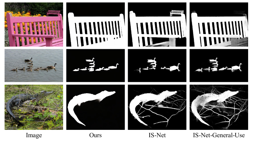
Figure 10: Cross dataset comparison of our model and other models.

Failure Cases of DIS. Our method also has some limitations. For Instance, it may fail to generate accurate foreground masks when the foreground and background colors are similar. As shown in Fig. 11 (a) and (b), when encountering camouflaged objects, the model cannot produce a complete mask for the camouflaged parts whose colors blend into the background. Additionally, the segmentation granularity of the model may not always align with the ground truth, especially when there are multiple feasible segmentation results for foreground objects in the image. As shown in Fig. 11 (c), the model predicts a mask for just the chairs and the flowerpot while the ground truth mask treats the chairs, the flowerpot, and the swing as one integral whole.

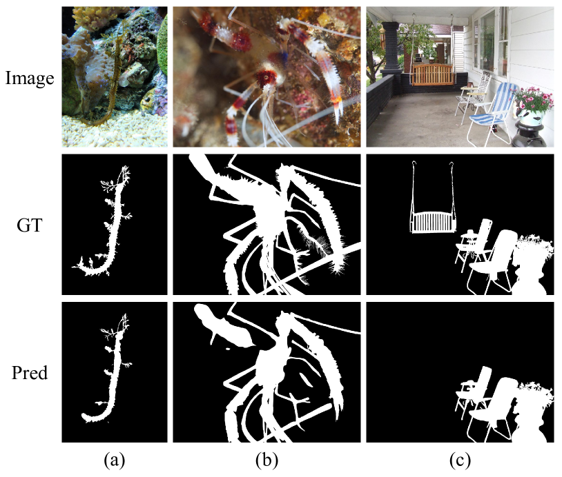
Figure 11: Typical failure cases.

0.B.4 Image Matting

More Qualitative Evaluation. In Fig. 15, we showcase more qualitative results for the image matting task. It is worth noting that our model works well in various resolutions, light environments, human poses, and human orientations. Please zoom in for better visualization and more details.

0.B.5 Human Pose Estimation

More Qualitative Evaluation. In Fig.16, we showcase more qualitative results for the human pose estimation. We conduct experiments on MHP dataset[45], and we use mmpose[15] to render the human pose following the setting of [5].

0.B.6 Anomaly Detection

Task Definition Anomaly detection refers to the analytical process of scrutinizing individual data points to identify uncommon events or observations. The focus of anomaly detection lies in its capacity to discern subtle irregularities within a dataset, which are often indicative of critical, underlying issues.

Datasets MVTec AD [7] is a benchmark dataset specialized for evaluating anomaly detection techniques, particularly in industrial inspection contexts. It includes more than 5000 high-resolution images across 15 diverse categories of objects and textures. For each category, the dataset provides defect-free images for training and a test set that includes both defective and non-defective images.

Evaluation Our experiments show that our method reaches 91.97% pixel AUC on MVTec AD [7], Fig. 17 demonstrates the qualitative results.

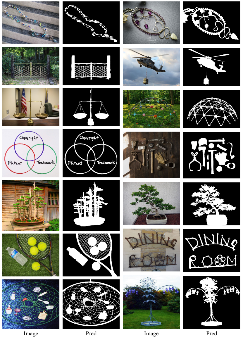
Figure 14: Qualitative results of dichotomous image segmentation.

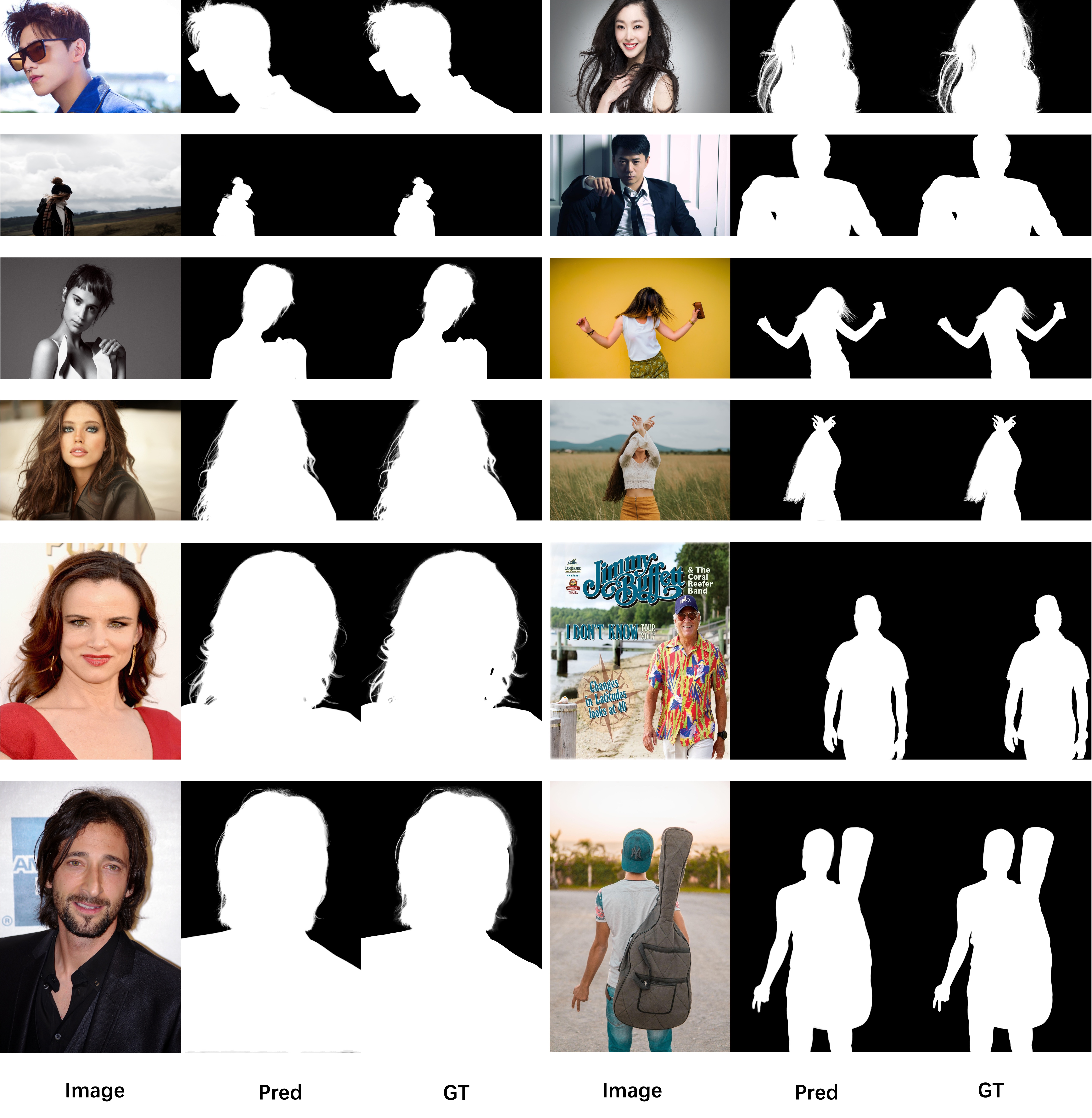
Figure 15: More qualitative results for image matting.

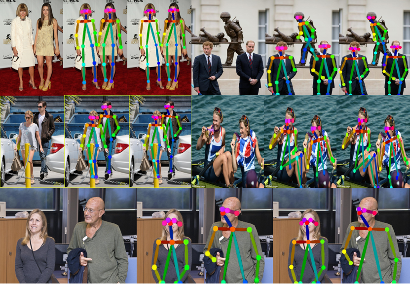
Figure 16: More qualitative results for human pose estimation. (Left: original Image, Mid: prediction, Right: ground truth)

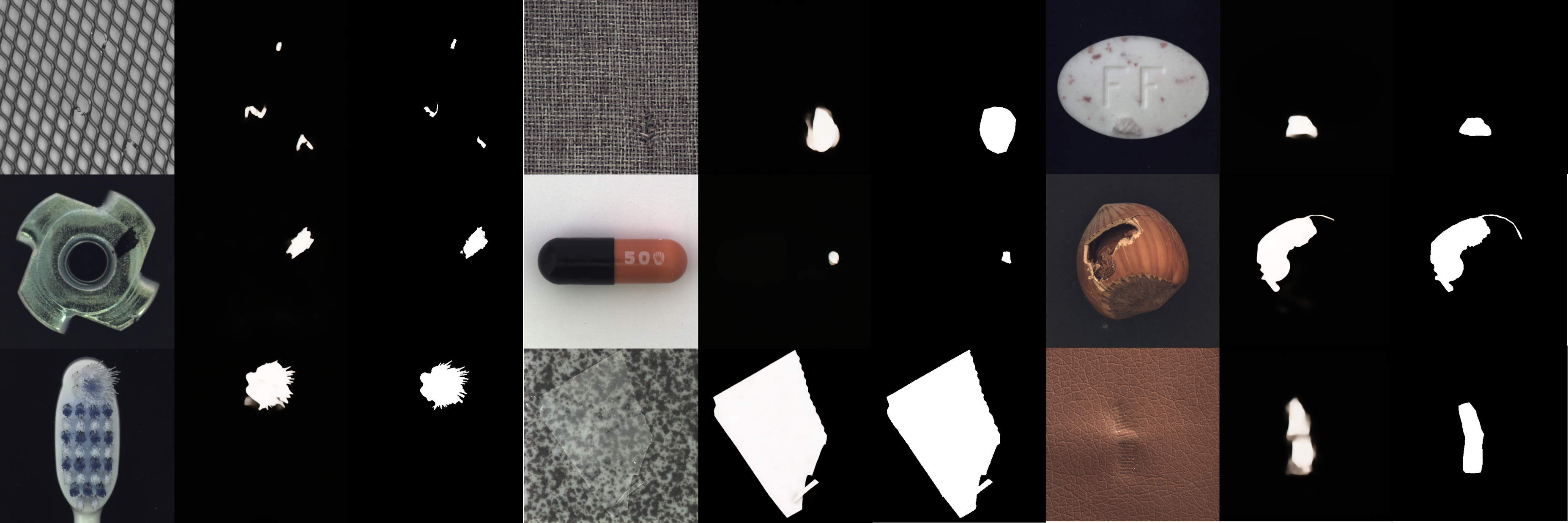
Figure 17: Defect Detection Results. (Left: original image, Middle: prediction, Right: ground truth)

References

- [1] Radhakrishna Achanta, Sheila Hemami, Francisco Estrada, and Sabine Susstrunk. Frequency-tuned salient region detection. In Proc. IEEE Conf. Comp. Vis. Patt. Recogn., 2009.
- [2] Eirikur Agustsson and Radu Timofte. Ntire 2017 challenge on single image super-resolution: Dataset and study. In IEEE Conf. Ccomputer Vision and Pattern Recognition Workshops, 2017.
- [3] Gwangbin Bae, Ignas Budvytis, and Roberto Cipolla. Estimating and exploiting the aleatoric uncertainty in surface normal estimation. In Proc. IEEE Int. Conf. Comp. Vis., 2021.
- [4] Gwangbin Bae and Andrew J Davison. Rethinking inductive biases for surface normal estimation. arXiv preprint arXiv:2403.00712, 2024.
- [5] Yutong Bai, Xinyang Geng, Karttikeya Mangalam, Amir Bar, Alan Yuille, Trevor Darrell, Jitendra Malik, and Alexei A Efros. Sequential modeling enables scalable learning for large vision models. arXiv: Comp. Res. Repository, 2023.
- [6] Arpit Bansal, Eitan Borgnia, Hong-Min Chu, Jie Li, Hamid Kazemi, Furong Huang, Micah Goldblum, Jonas Geiping, and Tom Goldstein. Cold diffusion: Inverting arbitrary image transforms without noise. Proc. Advances in Neural Inf. Process. Syst., 2024.
- [7] Paul Bergmann, Kilian Batzner, Michael Fauser, David Sattlegger, and Carsten Steger. The mvtec anomaly detection dataset: a comprehensive real-world dataset for unsupervised anomaly detection. Int. J. Comput. Vision, 2021.
- [8] Anand Bhattad, Daniel McKee, Derek Hoiem, and David Forsyth. Stylegan knows normal, depth, albedo, and more. Proc. Advances in Neural Inf. Process. Syst., 2024.
- [9] Jake Bruce, Michael Dennis, Ashley Edwards, Jack Parker-Holder, Yuge Shi, Edward Hughes, Matthew Lai, Aditi Mavalankar, Richie Steigerwald, Chris Apps, et al. Genie: Generative interactive environments. arXiv: Comp. Res. Repository, 2024.
- [10] Junsong Chen, YU Jincheng, GE Chongjian, Lewei Yao, Enze Xie, Zhongdao Wang, James Kwok, Ping Luo, Huchuan Lu, and Zhenguo Li. Pixart-: Fast training of diffusion transformer for photorealistic text-to-image synthesis. In Proc. Int. Conf. Learn. Representations, 2023.
- [11] Liang-Chieh Chen, Yukun Zhu, George Papandreou, Florian Schroff, and Hartwig Adam. Encoder-decoder with atrous separable convolution for semantic image segmentation. In Proc. Eur. Conf. Comp. Vis., 2018.
- [12] Zuyao Chen, Qianqian Xu, Runmin Cong, and Qingming Huang. Global context-aware progressive aggregation network for salient object detection. In Proc. AAAI Conf. Artificial Intell., 2020.
- [13] Aakanksha Chowdhery, Sharan Narang, Jacob Devlin, Maarten Bosma, Gaurav Mishra, Adam Roberts, Paul Barham, Hyung Won Chung, Charles Sutton, Sebastian Gehrmann, et al. Palm: Scaling language modeling with pathways. J. Mach. Learn. Res., 2023.
- [14] Djork-Arné Clevert, Thomas Unterthiner, and Sepp Hochreiter. Fast and accurate deep network learning by exponential linear units (elus). In Proc. Int. Conf. Learn. Representations, 2016.
- [15] MMPose Contributors. Openmmlab pose estimation toolbox and benchmark. https://github.com/open-mmlab/mmpose, 2020.
- [16] Angela Dai, Angel X Chang, Manolis Savva, Maciej Halber, Thomas Funkhouser, and Matthias Nießner. Scannet: Richly-annotated 3d reconstructions of indoor scenes. In Proc. IEEE Conf. Comp. Vis. Patt. Recogn., 2017.
- [17] Jia Deng, Wei Dong, Richard Socher, Li-Jia Li, Kai Li, and Li Fei-Fei. Imagenet: A large-scale hierarchical image database. In arXiv: Comp. Res. Repository, 2009.
- [18] Tien Do, Khiem Vuong, Stergios I Roumeliotis, and Hyun Soo Park. Surface normal estimation of tilted images via spatial rectifier. In Proc. Eur. Conf. Comp. Vis., 2020.
- [19] Alexey Dosovitskiy, Lucas Beyer, Alexander Kolesnikov, Dirk Weissenborn, Xiaohua Zhai, Thomas Unterthiner, Mostafa Dehghani, Matthias Minderer, Georg Heigold, Sylvain Gelly, et al. An image is worth 16x16 words: Transformers for image recognition at scale. In Proc. Int. Conf. Learn. Representations, 2021.
- [20] Xiaodan Du, Nicholas Kolkin, Greg Shakhnarovich, and Anand Bhattad. Generative models: What do they know? do they know things? let’s find out! arXiv: Comp. Res. Repository, 2023.
- [21] Ainaz Eftekhar, Alexander Sax, Jitendra Malik, and Amir Zamir. Omnidata: A scalable pipeline for making multi-task mid-level vision datasets from 3d scans. In Proc. IEEE Int. Conf. Comp. Vis., 2021.
- [22] David Eigen, Christian Puhrsch, and Rob Fergus. Depth map prediction from a single image using a multi-scale deep network. Advances in neural information processing systems, 27, 2014.
- [23] Alaaeldin El-Nouby, Michal Klein, Shuangfei Zhai, Miguel Angel Bautista, Alexander Toshev, Vaishaal Shankar, Joshua M Susskind, and Armand Joulin. Scalable pre-training of large autoregressive image models. arXiv: Comp. Res. Repository, 2024.
- [24] D Fan, M Cheng, Y Liu, T Li, and A Borji. A new way to evaluate foreground maps. In Proc. IEEE Conf. Comp. Vis. Patt. Recogn., 2017.
- [25] Deng-Ping Fan, Cheng Gong, Yang Cao, Bo Ren, Ming-Ming Cheng, and Ali Borji. Enhanced-alignment measure for binary foreground map evaluation. In Proc. International Joint Conf. Artificial Intelligence, 2018.
- [26] Deng-Ping Fan, Ge-Peng Ji, Ming-Ming Cheng, and Ling Shao. Concealed object detection. IEEE Trans. Pattern Anal. Mach. Intell., 2021.
- [27] Deng-Ping Fan, Ge-Peng Ji, Xuebin Qin, and Ming-Ming Cheng. Cognitive vision inspired object segmentation metric and loss function. Scientia Sinica Informationis, 2021.
- [28] Mingyuan Fan, Shenqi Lai, Junshi Huang, Xiaoming Wei, Zhenhua Chai, Junfeng Luo, and Xiaolin Wei. Rethinking bisenet for real-time semantic segmentation. In Proc. IEEE Conf. Comp. Vis. Patt. Recogn., 2021.
- [29] Andreas Geiger, Philip Lenz, Christoph Stiller, and Raquel Urtasun. Vision meets robotics: The kitti dataset. Int. J. Robotics Research, 2013.
- [30] Xavier Glorot, Antoine Bordes, and Yoshua Bengio. Deep sparse rectifier neural networks. In Proceedings of the fourteenth international conference on artificial intelligence and statistics, pages 315–323. JMLR Workshop and Conference Proceedings, 2011.
- [31] Kaiming He, Xinlei Chen, Saining Xie, Yanghao Li, Piotr Dollár, and Ross Girshick. Masked autoencoders are scalable vision learners. In Proc. IEEE Conf. Comp. Vis. Patt. Recogn., 2022.
- [32] Kaiming He, Haoqi Fan, Yuxin Wu, Saining Xie, and Ross Girshick. Momentum contrast for unsupervised visual representation learning. In Proc. IEEE Conf. Comp. Vis. Patt. Recogn., 2020.
- [33] Kaiming He, Xiangyu Zhang, Shaoqing Ren, and Jian Sun. Deep residual learning for image recognition. In Proc. IEEE Conf. Comp. Vis. Patt. Recogn., 2016.
- [34] Jonathan Ho, Ajay Jain, and Pieter Abbeel. Denoising diffusion probabilistic models. Proc. Advances in Neural Inf. Process. Syst., 2020.
- [35] Jordan Hoffmann, Sebastian Borgeaud, Arthur Mensch, Elena Buchatskaya, Trevor Cai, Eliza Rutherford, Diego de Las Casas, Lisa Anne Hendricks, Johannes Welbl, Aidan Clark, et al. Training compute-optimal large language models. arXiv: Comp. Res. Repository, 2022.
- [36] Andrew Howard, Mark Sandler, Grace Chu, Liang-Chieh Chen, Bo Chen, Mingxing Tan, Weijun Wang, Yukun Zhu, Ruoming Pang, Vijay Vasudevan, et al. Searching for mobilenetv3. In Proc. IEEE Int. Conf. Comp. Vis., 2019.
- [37] Edward J Hu, Yelong Shen, Phillip Wallis, Zeyuan Allen-Zhu, Yuanzhi Li, Shean Wang, Lu Wang, and Weizhu Chen. LoRA: Low-rank adaptation of large language models. In Proc. Int. Conf. Learn. Representations, 2022.
- [38] Jingwei Huang, Yichao Zhou, Thomas Funkhouser, and Leonidas J Guibas. Framenet: Learning local canonical frames of 3d surfaces from a single rgb image. In Proc. IEEE Int. Conf. Comp. Vis., 2019.
- [39] Bingxin Ke, Anton Obukhov, Shengyu Huang, Nando Metzger, Rodrigo Caye Daudt, and Konrad Schindler. Repurposing diffusion-based image generators for monocular depth estimation. arXiv: Comp. Res. Repository, 2023.
- [40] Diederik P Kingma and Max Welling. Auto-encoding variational Bayes. In Proc. Int. Conf. Learn. Representations, 2014.
- [41] Alexander Kirillov, Eric Mintun, Nikhila Ravi, Hanzi Mao, Chloe Rolland, Laura Gustafson, Tete Xiao, Spencer Whitehead, Alexander C. Berg, Wan-Yen Lo, Piotr Dollár, and Ross Girshick. Segment anything. Proc. IEEE Int. Conf. Comp. Vis., 2023.
- [42] Lubor Ladicky, Bernhard Zeisl, and Marc Pollefeys. Discriminatively trained dense surface normal estimation. In Proc. Eur. Conf. Comp. Vis., 2014.
- [43] Hsin-Ying Lee, Hung-Yu Tseng, and Ming-Hsuan Yang. Exploiting diffusion prior for generalizable pixel-level semantic prediction. arXiv: Comp. Res. Repository, 2023.
- [44] Jizhizi Li, Sihan Ma, Jing Zhang, and Dacheng Tao. Privacy-preserving portrait matting. In Proc. ACM Int. Conf. Multimedia, 2021.
- [45] Jianshu Li, Jian Zhao, Yunchao Wei, Congyan Lang, Yidong Li, Terence Sim, Shuicheng Yan, and Jiashi Feng. Multiple-human parsing in the wild. arXiv preprint arXiv: 1705.07206, 2017.
- [46] Tsung-Yi Lin, Michael Maire, Serge Belongie, James Hays, Pietro Perona, Deva Ramanan, Piotr Dollár, and C Lawrence Zitnick. Microsoft coco: Common objects in context. In Proc. Eur. Conf. Comp. Vis., 2014.
- [47] Ran Margolin, Lihi Zelnik-Manor, and Ayellet Tal. How to evaluate foreground maps? In Proc. IEEE Conf. Comp. Vis. Patt. Recogn., 2014.
- [48] Haiyang Mei, Ge-Peng Ji, Ziqi Wei, Xin Yang, Xiaopeng Wei, and Deng-Ping Fan. Camouflaged object segmentation with distraction mining. In Proc. IEEE Conf. Comp. Vis. Patt. Recogn., 2021.
- [49] Yuval Nirkin, Lior Wolf, and Tal Hassner. Hyperseg: Patch-wise hypernetwork for real-time semantic segmentation. In Proc. IEEE Conf. Comp. Vis. Patt. Recogn., 2021.
- [50] openai. GPT-4V(ision) technical work and authors. Technical report, 2023.
- [51] Maxime Oquab, Timothée Darcet, Théo Moutakanni, Huy Vo, and Marc Szafraniec et al. DINOv2: Learning robust visual features without supervision. Trans. Mach. Learn. Research, 2024.
- [52] Federico Perazzi, Philipp Krähenbühl, Yael Pritch, and Alexander Hornung. Saliency filters: Contrast based filtering for salient region detection. In Proc. IEEE Conf. Comp. Vis. Patt. Recogn., 2012.
- [53] Lu Qi, Lehan Yang, Weidong Guo, Yu Xu, Bo Du, Varun Jampani, and Ming-Hsuan Yang. Unigs: Unified representation for image generation and segmentation. arXiv: Comp. Res. Repository, 2023.
- [54] Xuebin Qin, Hang Dai, Xiaobin Hu, Deng-Ping Fan, Ling Shao, and Luc Van Gool. Highly accurate dichotomous image segmentation. In Proc. Eur. Conf. Comp. Vis., 2022.
- [55] Xuebin Qin, Zichen Zhang, Chenyang Huang, Masood Dehghan, Osmar R Zaiane, and Martin Jagersand. U2-net: Going deeper with nested u-structure for salient object detection. Pattern Recogn., 2020.
- [56] Xuebin Qin, Zichen Zhang, Chenyang Huang, Chao Gao, Masood Dehghan, and Martin Jagersand. Basnet: Boundary-aware salient object detection. In Proc. IEEE Conf. Comp. Vis. Patt. Recogn., 2019.
- [57] Alec Radford, Jong Wook Kim, Chris Hallacy, Aditya Ramesh, Gabriel Goh, Sandhini Agarwal, Girish Sastry, Amanda Askell, Pamela Mishkin, Jack Clark, et al. Learning transferable visual models from natural language supervision. In Proc. Int. Conf. Mach. Learn., 2021.
- [58] Alec Radford, Jeffrey Wu, Rewon Child, David Luan, Dario Amodei, Ilya Sutskever, et al. Language models are unsupervised multitask learners. OpenAI Blog, 2019.
- [59] Colin Raffel, Noam Shazeer, Adam Roberts, Katherine Lee, Sharan Narang, Michael Matena, Yanqi Zhou, Wei Li, Peter J Liu, et al. Exploring the limits of transfer learning with a unified text-to-text transformer. J. Mach. Learn. Res., 2020.
- [60] René Ranftl, Alexey Bochkovskiy, and Vladlen Koltun. Vision transformers for dense prediction. In Proc. IEEE Int. Conf. Comp. Vis., 2021.
- [61] René Ranftl, Katrin Lasinger, David Hafner, Konrad Schindler, and Vladlen Koltun. Towards robust monocular depth estimation: Mixing datasets for zero-shot cross-dataset transfer. IEEE Trans. Pattern Anal. Mach. Intell., 2020.
- [62] Mike Roberts, Jason Ramapuram, Anurag Ranjan, Atulit Kumar, Miguel Angel Bautista, Nathan Paczan, Russ Webb, and Joshua M. Susskind. Hypersim: A photorealistic synthetic dataset for holistic indoor scene understanding. In Proc. IEEE Int. Conf. Comp. Vis., 2021.
- [63] Robin Rombach, Andreas Blattmann, Dominik Lorenz, Patrick Esser, and Bjorn Ommer. High-resolution image synthesis with latent diffusion models. In Proc. IEEE Conf. Comp. Vis. Patt. Recogn., 2022.
- [64] Olaf Ronneberger, Philipp Fischer, and Thomas Brox. U-net: Convolutional networks for biomedical image segmentation. In Proc. Medical Image Computing and Computer-Assisted Intervention, 2015.
- [65] Tim Salimans and Jonathan Ho. Progressive distillation for fast sampling of diffusion models. In Proc. Int. Conf. Learn. Representations, 2021.
- [66] Thomas Schops, Johannes L Schonberger, Silvano Galliani, Torsten Sattler, Konrad Schindler, Marc Pollefeys, and Andreas Geiger. A multi-view stereo benchmark with high-resolution images and multi-camera videos. In Proc. IEEE Conf. Comp. Vis. Patt. Recogn., 2017.
- [67] Christoph Schuhmann, Romain Beaumont, Richard Vencu, Cade Gordon, Ross Wightman, Mehdi Cherti, Theo Coombes, Aarush Katta, Clayton Mullis, Mitchell Wortsman, Patrick Schramowski, Srivatsa Kundurthy, Katherine Crowson, Ludwig Schmidt, Robert Kaczmarczyk, and Jenia Jitsev. LAION-5B: An open large-scale dataset for training next generation image-text models. Proc. Advances in Neural Inf. Process. Syst., 2022.
- [68] Shuai Shao, Zeming Li, Tianyuan Zhang, Chao Peng, Gang Yu, Xiangyu Zhang, Jing Li, and Jian Sun. Objects365: A large-scale, high-quality dataset for object detection. In Proc. IEEE Int. Conf. Comp. Vis., 2019.
- [69] Nathan Silberman, Derek Hoiem, Pushmeet Kohli, and Rob Fergus. Indoor segmentation and support inference from rgbd images. In Proc. Eur. Conf. Comp. Vis., 2012.
- [70] Jiaming Song, Chenlin Meng, and Stefano Ermon. Denoising diffusion implicit models. In Proc. Int. Conf. Learn. Representations, 2020.
- [71] Hugo Touvron, Thibaut Lavril, Gautier Izacard, Xavier Martinet, Marie-Anne Lachaux, Timothée Lacroix, Baptiste Rozière, Naman Goyal, Eric Hambro, Faisal Azhar, Aurelien Rodriguez, Armand Joulin, Edouard Grave, and Guillaume Lample. LLaMA: Open and efficient foundation language models. arXiv: Comp. Res. Repository, 2023.
- [72] Wouter Van Gansbeke and Bert De Brabandere. A simple latent diffusion approach for panoptic segmentation and mask inpainting. arXiv: Comp. Res. Repository, 2024.
- [73] Igor Vasiljevic, Nick Kolkin, Shanyi Zhang, Ruotian Luo, Haochen Wang, Falcon Z. Dai, Andrea F. Daniele, Mohammadreza Mostajabi, Steven Basart, Matthew R. Walter, and Gregory Shakhnarovich. DIODE: A Dense Indoor and Outdoor DEpth Dataset. arXiv: Comp. Res. Repository, 2019.
- [74] Jingdong Wang, Ke Sun, Tianheng Cheng, Borui Jiang, Chaorui Deng, Yang Zhao, Dong Liu, Yadong Mu, Mingkui Tan, Xinggang Wang, et al. Deep high-resolution representation learning for visual recognition. IEEE Trans. Pattern Anal. Mach. Intell., 2020.
- [75] Rui Wang, David Geraghty, Kevin Matzen, Richard Szeliski, and Jan-Michael Frahm. Vplnet: Deep single view normal estimation with vanishing points and lines. In Proc. IEEE Conf. Comp. Vis. Patt. Recogn., 2020.
- [76] Xinlong Wang, Wen Wang, Yue Cao, Chunhua Shen, and Tiejun Huang. Images speak in images: A generalist painter for in-context visual learning. In Proc. IEEE Conf. Comp. Vis. Patt. Recogn., 2023.
- [77] Jun Wei, Shuhui Wang, and Qingming Huang. F3net: fusion, feedback and focus for salient object detection. In Proc. AAAI Conf. Artificial Intell., 2020.
- [78] Weilai Xiang, Hongyu Yang, Di Huang, and Yunhong Wang. Denoising diffusion autoencoders are unified self-supervised learners. In Proc. IEEE Int. Conf. Comp. Vis., 2023.
- [79] Bin Xiao, Haiping Wu, and Yichen Wei. Simple baselines for human pose estimation and tracking. In Proc. Eur. Conf. Comp. Vis., 2018.
- [80] Tete Xiao, Yingcheng Liu, Bolei Zhou, Yuning Jiang, and Jian Sun. Unified perceptual parsing for scene understanding. In Proc. Eur. Conf. Comp. Vis., 2018.
- [81] Yufei Xu, Jing Zhang, Qiming Zhang, and Dacheng Tao. ViTPose: Simple vision transformer baselines for human pose estimation. In Proc. Advances in Neural Inf. Process. Syst., 2022.
- [82] Wei Yin, Yifan Liu, Chunhua Shen, and Youliang Yan. Enforcing geometric constraints of virtual normal for depth prediction. In Proc. IEEE Int. Conf. Comp. Vis., 2019.
- [83] Wei Yin, Xinlong Wang, Chunhua Shen, Yifan Liu, Zhi Tian, Songcen Xu, Changming Sun, and Dou Renyin. Diversedepth: Affine-invariant depth prediction using diverse data. arXiv: Comp. Res. Repository, 2020.
- [84] Wei Yin, Jianming Zhang, Oliver Wang, Simon Niklaus, Long Mai, Simon Chen, and Chunhua Shen. Learning to recover 3d scene shape from a single image. In Proc. IEEE Conf. Comp. Vis. Patt. Recogn., 2021.
- [85] Changqian Yu, Jingbo Wang, Chao Peng, Changxin Gao, Gang Yu, and Nong Sang. Bisenet: Bilateral segmentation network for real-time semantic segmentation. In Proc. Eur. Conf. Comp. Vis., 2018.
- [86] Jiahui Yu, Zirui Wang, Vijay Vasudevan, Legg Yeung, Mojtaba Seyedhosseini, and Yonghui Wu. Coca: Contrastive captioners are image-text foundation models. Trans. Machine Learning Research, 2022.
- [87] Chi Zhang, Wei Yin, Billzb Wang, Gang Yu, Bin Fu, and Chunhua Shen. Hierarchical normalization for robust monocular depth estimation. Proc. Advances in Neural Inf. Process. Syst., 2022.
- [88] Hao Zhang, Feng Li, Shilong Liu, Lei Zhang, Hang Su, Jun Zhu, Lionel Ni, and Heung-Yeung Shum. Dino: Detr with improved denoising anchor boxes for end-to-end object detection. In Proc. Int. Conf. Learn. Representations, 2022.
- [89] Lvmin Zhang, Anyi Rao, and Maneesh Agrawala. Adding conditional control to text-to-image diffusion models. In Proceedings of the IEEE/CVF International Conference on Computer Vision, pages 3836–3847, 2023.
- [90] Hengshuang Zhao, Xiaojuan Qi, Xiaoyong Shen, Jianping Shi, and Jiaya Jia. Icnet for real-time semantic segmentation on high-resolution images. In Proc. Eur. Conf. Comp. Vis., 2018.
- [91] Hengshuang Zhao, Jianping Shi, Xiaojuan Qi, Xiaogang Wang, and Jiaya Jia. Pyramid scene parsing network. In Proc. IEEE Conf. Comp. Vis. Patt. Recogn., 2017.
- [92] Xiaoqi Zhao, Youwei Pang, Lihe Zhang, Huchuan Lu, and Lei Zhang. Suppress and balance: A simple gated network for salient object detection. In Proc. Eur. Conf. Comp. Vis., 2020.
- [93] Bolei Zhou, Hang Zhao, Xavier Puig, Sanja Fidler, Adela Barriuso, and Antonio Torralba. Scene parsing through ade20k dataset. In Proc. IEEE Conf. Comp. Vis. Patt. Recogn., 2017.