pETNNs: Partial Evolutionary Tensor Neural Networks for Solving Time-dependent Partial Differential Equations

Abstract

We present partial evolutionary tensor neural networks (pETNNs), a novel framework for solving time-dependent partial differential equations with both of high accuracy and remarkable extrapolation. Our proposed architecture leverages the inherent accuracy of tensor neural networks, while incorporating evolutionary parameters that enable remarkable extrapolation capabilities. By adopting innovative parameter update strategies, the pETNNs achieve a significant reduction in computational cost while maintaining precision and robustness. Notably, the pETNNs enhance the accuracy of conventional evolutional deep neural networks and empowers computational abilities to address high-dimensional problems. Numerical experiments demonstrate the superior performance of the pETNNs in solving time-dependent complex equations, including the Navier-Stokes equations, high-dimensional heat equation, high-dimensional transport equation and Korteweg-de Vries type equation.

Keywords. time-dependent partial differential equations, tensor neural networks, evolutional deep neural networks, partial evolutionary tensor neural networks, high-dimensional problems.

1 Introduction

Partial differential equations (PDEs) are ubiquitous in modeling phenomena across scientific and engineering disciplines. They serve as indispensable tools in the modeling of continuum mechanics, electromagnetic theory, quantum mechanics, and a myriad of other fields where the evolution of systems across space and time is of interest. Traditional numerical approaches for solving PDEs, such as finite difference [14], finite element [4], and spectral methods [22], have been widely used. However, the computational burden imposed by these methods grows exponentially with the increase in dimensionality of the problem, often rendering them impractical for high-dimensional systems. This phenomenon, known as the “curse of dimensionality”, has been a persistent impediment to progress in various scientific domains.

The emergence of machine learning has introduced a novel set of tools to the scientific community, offering a potential panacea to the curse of dimensionality. Deep learning, a class of machine learning characterized by deep neural networks (DNNs), has been particularly successful in areas where traditional algorithms falter due to the complexity and volume of the data involved, such as [6, 13, 16, 17]. The universal approximation theorem underpins this capability, suggesting that a neural network can approximate any continuous function to a desired degree of accuracy [5, 10]. Leveraging this, researchers have proposed various frameworks where DNNs are trained to satisfy the differential operators, initial conditions, and boundary conditions of PDEs.

A notable advancement in the field is the emergence of deep Galerkin method (DGM) [23], deep Ritz method (DRM) [8], and particularly physics-informed neural networks (PINNs) [21]. They embed the governing physical laws, encapsulated by PDEs, into the architecture of deep learning models. By incorporating the PDEs directly into the loss function, PINNs ensure that the learned solutions are not merely data-driven but also conform to the underlying physical principles. This integration of physical laws into the learning process imbues PINNs with the ability to generalize beyond the data they were trained on, making them particularly adept at handling scenarios where data is scarce or expensive to acquire.

However, the efficacy of PINNs is predominantly confined to the temporal domain for which they have been trained, typically within the interval $[0,T]$. Their ability to extrapolate beyond this training window is limited, which is a manifestation of neural networks’ inherent weakness in out-of-distribution (OOD) generalization. This limitation hinders their predictive capacity, rendering them less effective for forecasting future states of the system under study.

The evolutional deep neural networks (EDNNs) [7], which can address this challenge, have been developed as an innovative approach to solve time-dependent PDEs. The EDNNs are designed to evolve in tandem with the temporal dynamics they model, thus possessing an enhanced capability for prediction. This is achieved by structuring the neural network in a way that it intrinsically accounts for the temporal evolution, allowing for a more robust extrapolation into future times. The methodology derived by the EDNNs has attracted significant attention. The authors in [3] employed this to build upon the foundational results established in [1]. Specifically, they move away from the traditional method of training DNNs for PDEs and adopt a new strategy that uses the Dirac-Frenkel variational principle to evolve the network parameters through a system of ordinary differential equations (ODEs). Subsequently, they have enhanced its computational efficiency by randomized sparse neural Galerkin schemes in [2]. Furthermore, the authors in [12] conducted a comprehensive investigation into the boundary treatment of EDNNs, leading to significant improvements.

Despite the method of the EDNNs can effectively compute the time-dependent PDEs and reasonably predict the related solutions, it seems unable to yield high-precision due to its reliance on the Monte Carlo approach in the process of computing integrals. On the other hand, many works that delve into various techniques aimed at improving the accuracy and efficiency of deep learning-based solver for PDEs, such as [11, 18, 25, 9, 19]. Among them, the tensor neural networks (TNNs) emerge as a methodological innovation [15, 26, 27], characterized by a restructured network architecture that can employ Gaussian quadrature formula as an alternative to Monte Carlo integration, thus substantially enhances the accuracy of solutions. Nonetheless, the current implementation of this approach is exclusively tailored to stationary partial differential equations, and its utilization in the context of time-dependent differential equations has not been studied in the extant scholarly discourse.

This paper advances the TNNs framework, endowing it with the augmented capacity for the computation of time-dependent equations with maintaining high accuracy. Furthermore, novel parameter update strategies (only update partial parameters) have been developed to optimize the allocation of computational resources. Thus, our work is named as partial evolutionary tensor neural networks (pETNNs, pronounced “$Peten$”). Numerical experiments show that pETNNs can significantly curtail computational cost without compromising the related accuracy. The numerical solutions obtained by pETNNs not only achieve higher accuracy than the conventional EDNNs but also demonstrate marked superiority in resolving the complexities of the Navier-Stokes equations, Korteweg-de Vries (KdV) type equation, high-dimensional heat equation, and high-dimensional transport equation.

This paper is organized as follows. We propose the main results about the pETNNs in Section 2, including the derivation process, and the corresponding algorithms. Extensive numerical experiments are carried out to validate the efficiency of the proposed pETNNs in Section 3. We finally present our conclusion and discussion in Section 4.

2 Partial Evolutionary Tensor Neural Networks

In this section, we will show the structure and derivation of pETNNs. Before this, TNNs proposed in [26] are introduced, which are mainly designed for solving stationary PDEs.

2.1 Tensor Neural Networks

For clarity, we primarily discuss the method of approximating a scalar function using the TNNs, and it should be noted that the approach can be extended to high-dimensional cases straightforwardly. The function $u(x)$ is approximated by the TNNs as follows:

$$u(x;\theta)=\sum_{j=1}^{p}u_{1,j}\left(x_{1};\theta_{1}\right)u_{2,j}\left(x_{2};\theta_{2}\right)\cdots u_{d,j}\left(x_{d};\theta_{d}\right)=\sum_{j=1}^{p}\prod_{i=1}^{d}u_{i,j}\left(x_{i};\theta_{i}\right),$$ (2.1)

where $\theta=\{\theta_{1},\cdots,\theta_{d}\}$ denotes all parameters of the whole architecture. Fig. 1 shows the details about the TNNs which have $d$ sub-networks.

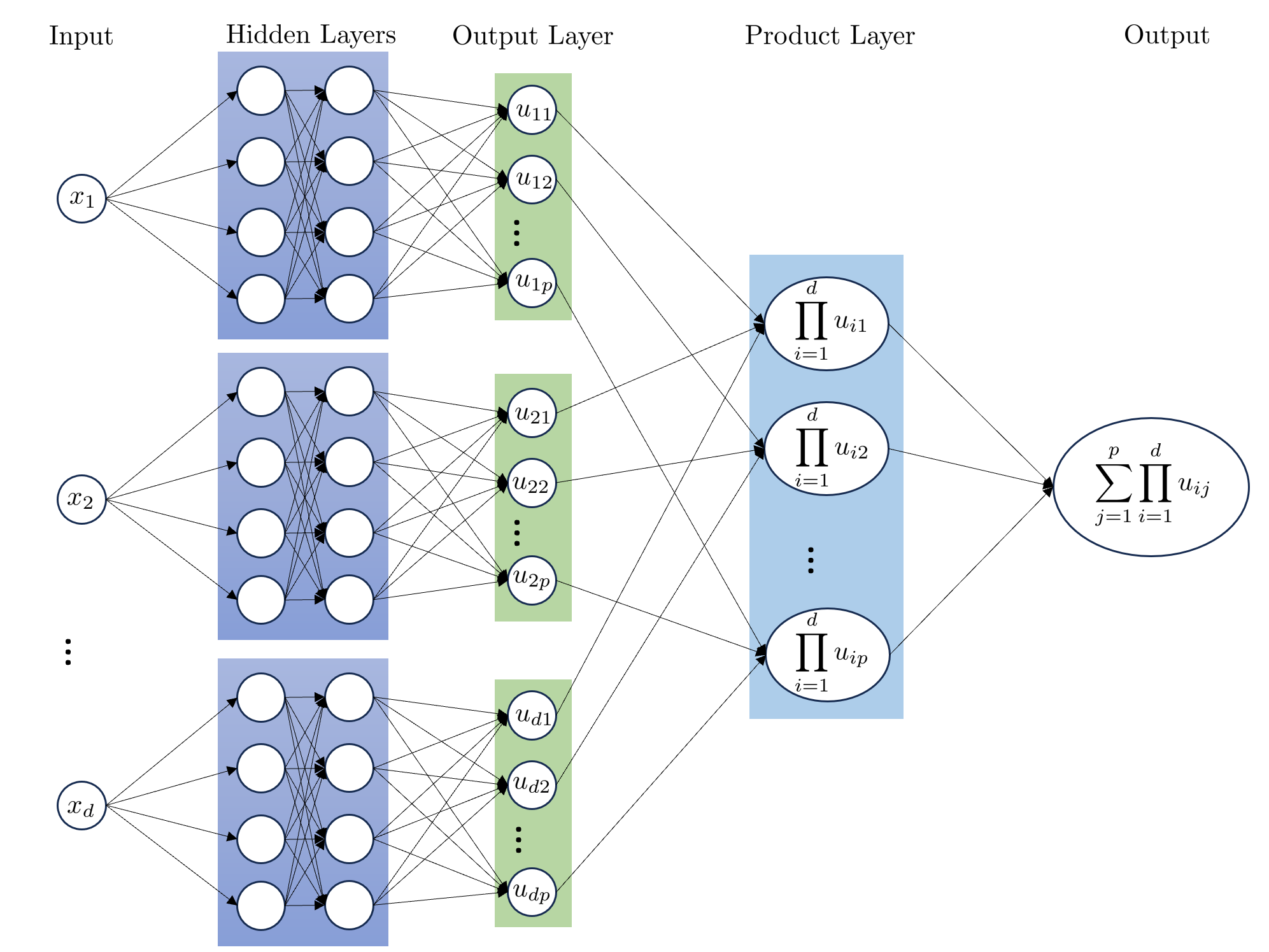
Figure 1: Schematic diagram of the tensor neural networks (TNNs).

One of the most advantages of the TNNs is that functions approximated by TNNs can be integrated using conventional Gaussian quadrature schemes, which offer higher precision compared to the Monte Carlo methods. This approach can be effectively incorporated into the formulation of loss functions, especially those based on the Mean Squared Error (MSE) criterion, thereby improving the precision of solutions to PDEs obtained via deep neural network frameworks. Furthermore, representing a function with the TNNs leads to a remarkable decrease in computational complexity for its numerical integration, which overcomes the curse of dimensionality in some sense. For a comprehensive discussion, refer to [26, 27].

2.2 Partial Evolutionary Tensor Neural Networks

We now provide a detailed introduction to the pETNNs for solving time-dependent PDEs, which is inspired by [7]. Here is the time-dependent general nonlinear partial differential equation,

$$\frac{\partial u}{\partial t}-\mathcal{N}(u) =0,\qquad(x,t)\in\Omega\times[0,T],$$ (2.2)

$$u(x,t=0) =u_{0}(x)$$

where $\Omega\subseteq\mathbb{R}^{d}$ denotes the spatial domain of the computation, $T$ represents the termination time for the simulation, $u=u(x,t)$ is the state function on both space and time, and $\mathcal{N}$ is a nonlinear differential operator. Fig. 2 shows the schematic diagram of the pETNNs. In this architecture, the embedding layer is used [24]. In this paper, the embedding for periodic boundary conditions is adopted as

$$x_{i}\rightarrow a[\cos(bx_{i}),\sin(bx_{i})],$$

where $a$ and $b$ are used to adjust the computational domain and the periodic frequency, respectively.

It is widely recognized that several prominent techniques for solving time-dependent PDEs with DNNs, such as the physics-informed neural network (PINN) [21], the deep Galerkin method (DGM) [23], and the deep Ritz method (DRM) [8], incorporate both time and spatial variables as inputs and have yielded impressive results. However, the structure of these methods is hard to make predictions beyond the training horizon. In order to forecast solutions without further training and achieve high accuracy, we propose the following pETNNs.

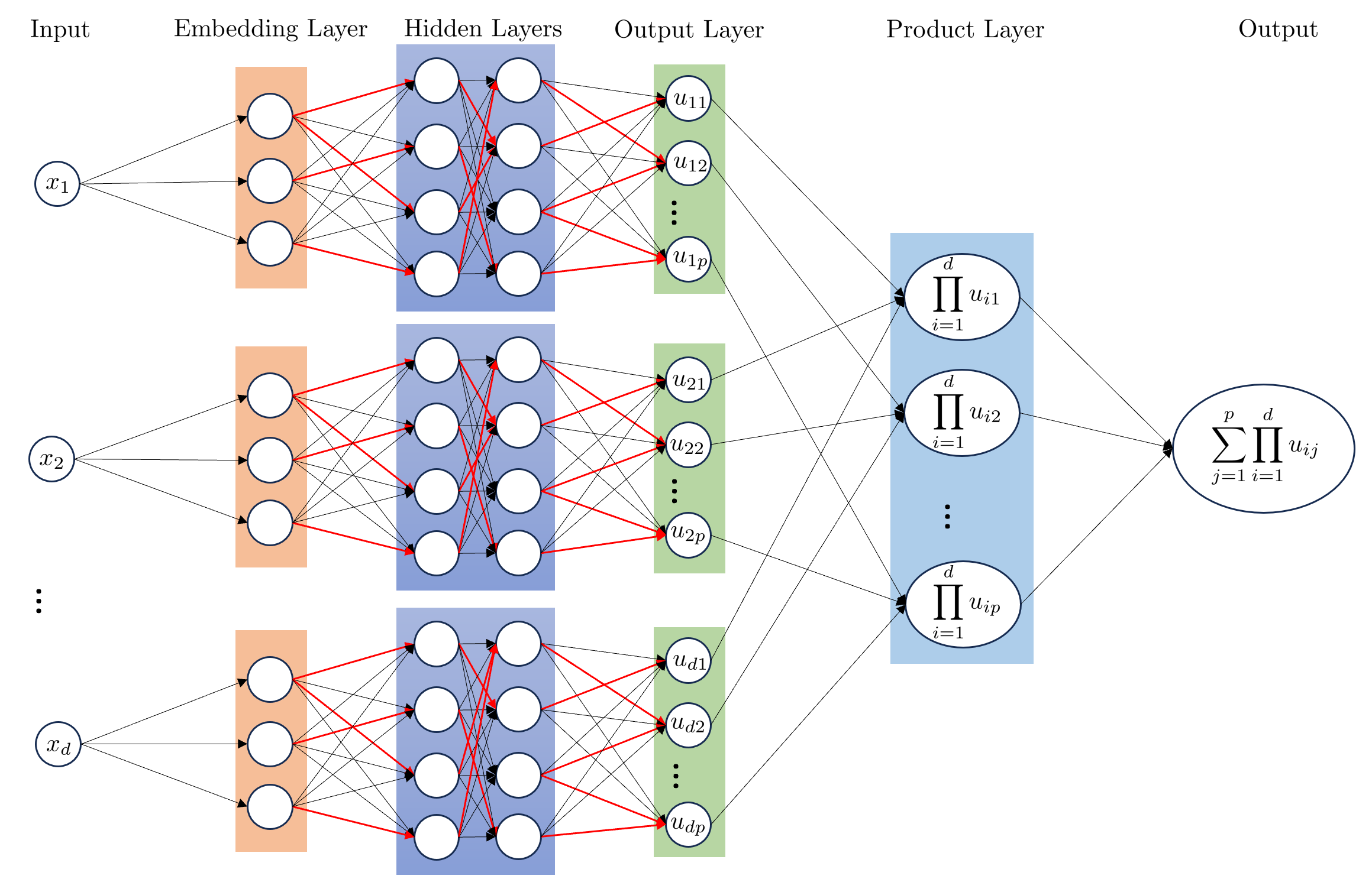
Figure 2: Schematic diagram of the partial evolutionary tensor neural networks (pETNNs). The thick red line represents the updated parameters and other parameters remain unchanged. The embedding layer is used.

As depicted in Fig. 2 and referred back to (2.1), the parameters are divided into two parts, constants (thin black lines) and time-varying variables (thick red lines), i.e., $\theta=\{\hat{\theta}(t),\tilde{\theta}\}$, and then we can obtain the approach,

$$\hat{u}(x,\theta(t))=\sum_{j=1}^{p}\prod_{i=1}^{d}\hat{u}_{i,j}\left(x_{i},\{\hat{\theta}_{i}(t),\tilde{\theta}_{i}\}\right).$$ (2.3)

In this context, the set $\{\hat{\theta}_{i}(t),\tilde{\theta}_{i}\}$ constitutes the collection of parameters associated with the $i$-th sub-network, where $\hat{\theta}_{i}(t)$ is designated as a function varying with time, and $\tilde{\theta}_{i}$ is time-independent.

The time derivative of solution $\hat{u}$ in (2.3) can be calculated by

$$\frac{\partial\hat{u}}{\partial t}=\frac{\partial\hat{u}}{\partial\hat{\theta}}\frac{d\hat{\theta}}{dt}.$$

Thus, to solve the PDE (2.2) is translated to find the solution to the optimization problem,

$$\frac{d\hat{\theta}}{dt} =\text{argmin}~{}J(\gamma),$$ (2.4)

$$\text{where}\quad J(\gamma) =\frac{1}{2}\int_{\Omega}\left|\frac{\partial\hat{u}}{\partial\hat{\theta}}\gamma-\mathcal{N}(\hat{u})\right|^{2}dx.$$

According to first-order optimality condition, the optimal solution $\gamma_{opt}$ to (2.4) satisfies

$$\left(\int_{\Omega}\left(\frac{\partial\hat{u}}{\partial\hat{\theta}}\right)^{T}\left(\frac{\partial\hat{u}}{\partial\hat{\theta}}\right)dx\right)\gamma_{opt}=\int_{\Omega}\frac{\partial\hat{u}^{T}}{\partial\hat{\theta}}\mathcal{N}(\hat{u})dx.$$ (2.5)

It should be pointed out that the first term on the left-hand side of the equation, inside the parentheses, is a matrix, whose $(i,j)$ entry is

$$\left(\int_{\Omega}\left(\frac{\partial\hat{u}}{\partial\hat{\theta}}\right)^{T}\left(\frac{\partial\hat{u}}{\partial\hat{\theta}}\right)dx\right)_{ij}=\left(\int_{\Omega}\frac{\partial\hat{u}}{\partial w_{i}}\frac{\partial\hat{u}}{\partial w_{j}}dx\right).$$ (2.6)

Here $w_{i}\in\hat{\theta}(t)$ is a specific neural network weight, and the corresponding derivative can be calculated by (2.3),

$$\frac{\partial\hat{u}}{\partial w_{i}} =\frac{\partial\sum_{j=1}^{p}\prod_{i=1}^{d}\hat{u}_{i,j}\left(x_{i},\hat{\theta}_{i}\right)}{\partial w_{i}}$$ (2.7)

$$=\sum_{j=1}^{p}\frac{\partial\hat{u}_{k,j}\left(x_{k},\hat{\theta}_{k}\right)}{\partial w_{i}}\prod_{i=1,i\neq k}^{d}\hat{u}_{i,j}\left(x_{i},\hat{\theta}_{i}\right)\qquad(\text{if}~{}~{}w_{i}\in\hat{\theta}_{k})$$

$$=:\sum_{j=1}^{p}\prod_{i=1}^{d}\check{u}_{i,j}\left(x_{i},\hat{\theta}_{i}\right),$$

The last line represents $\check{u}_{i,j}(x_{i},\hat{\theta}_{i})=\begin{cases}\frac{\partial\hat{u}_{k,j}\left(x_{k},\hat{\theta}_{k}\right)}{\partial w_{i}},&w_{i}\in\hat{\theta}_{k},\\ \hat{u}_{i,j}(x_{i},\hat{\theta}_{i}),&\text{others}.\end{cases}$

The optimal solution $\gamma_{opt}$ in (2.5) is solved by the least square method with an acceptable relative condition number. And according to (2.4), the parameters $\hat{\theta}(t)$ are evolved by traditional numerical methods, and in this paper, we use the predictor-corrector (modified-Euler) method.

$\bullet$ Predictive Step (explicit Euler method):

$$\hat{\theta}_{n}^{p}=\hat{\theta}_{n}+\Delta t\gamma_{opt}(\hat{\theta}_{n});$$

$\bullet$ Corrective Step (implicit Euler method):

$$\hat{\theta}_{n+1}=\hat{\theta}_{n}+\frac{\Delta t}{2}\left(\gamma_{opt}(\hat{\theta}_{n})+\gamma_{opt}(\hat{\theta}_{n}^{p})\right).$$

Here $\hat{\theta}_{n}=\hat{\theta}(n\Delta t)$ with $\Delta t$ the time step size and $n$ the index of time step.

In the initial phase of the procedure, we train the tensor neural networks, $\hat{u}(x,\theta(t))$, to approximate $u(x,t)$ at $t=0$. The implementation, including embedded constraints and Dirichlet boundary conditions, follows the methodology outlined in [7]. Specifically, we train the tensor neural network with a sufficient accuracy by the loss

$$\|\hat{u}(x,\theta_{0})-u_{0}(x)\|.$$

Here $\|*\|$ represents $L_{2}$ norm, which can be directly calculated by conventional Gaussian quadrature schemes in the TNNs architecture.

The entire procedure can be found delineated in Algorithm 1.

Algorithm 1 Partial Evolutionary Tensor Neural Networks with Fixed Parameter Update for Solving PDEs

1: Input: PDE (2.2) with boundary conditions and initial values, Gauss points and quadrature weights, tolerance for the least squares method, time step size $\Delta t$, computation time $T$

2: Output: Highly accurate solutions to the PDE (2.2) represented by the TNNs over the interval $[0,T]$

3:Randomly initialize the parameters $\theta$ of the TNNs

4:Train the TNNs to approximate $u(x,t=0)$ and obtain $\theta_{0}$

5:Partition $\theta_{0}$ into time-dependent $\hat{\theta}_{0}$ and time-independent $\tilde{\theta}$

6:while $t<T$ do

7:     Apply Automatic Differentiation (AD) to $\hat{\theta}_{n}$ in (2.7) and integrate (2.6) using the TNNs structure

8:     Solve for $\gamma_{\text{opt}}(\hat{\theta}_{n})$ in (2.5) by the least squares method

9:     Predictive step: $\hat{\theta}_{n}^{p}\leftarrow\hat{\theta}_{n}+\Delta t\gamma_{\text{opt}}(\hat{\theta}_{n})$

10:     Apply AD to $\hat{\theta}_{n}^{p}$ in (2.7) and integrate (2.6)

11:     Solve for $\gamma_{\text{opt}}(\hat{\theta}_{n}^{p})$ in (2.5) by the least squares method

12:     Corrective step: $\hat{\theta}_{n+1}\leftarrow\hat{\theta}_{n}+\frac{\Delta t}{2}(\gamma_{\text{opt}}(\hat{\theta}_{n})+\gamma_{\text{opt}}(\hat{\theta}_{n}^{p}))$

13:     Update and save parameters $\hat{\theta}_{n+1}$ and update the time $t$

14:end while

15:return The updated TNNs with parameters $\theta$ at time $T$

Noting that in the numerical solution of the ordinary differential equation (2.4), the iterative computation unfolds across a series of discrete temporal intervals. Within each interval, we can partition the parameter $\theta$ into time-dependent $\hat{\theta}$ and time-independent $\tilde{\theta}$. Therefore we present the corresponding Algorithm 2. It is noteworthy to mention that Algorithm 1 may be regarded as a particular instantiation of Algorithm 2, characterized by the constancy of parameters across successive time steps.

Algorithm 2 Partial Evolutionary Tensor Neural Networks with Randomized Parameter Update for Solving PDEs

1: Input: PDE (2.2) with boundary conditions and initial values, Gauss points and quadrature weights, tolerance for the least squares method, time step size $\Delta t$, computation time $T$

2: Output: Highly accurate solutions to the PDE (2.2) represented by the TNNs over the interval $[0,T]$

3:Randomly initialize the parameters $\theta$ of the TNNs

4:Train the TNNs to approximate $u(x,t=0)$ and obtain $\theta_{0}$

5:while $t<T$ do

6:     Partition $\theta_{n}$ randomly into time-dependent $\hat{\theta}_{n}$ and time-independent $\tilde{\theta}_{n}$

7:     Apply AD to $\hat{\theta}_{n}$ in (2.7) and integrate (2.6) using the TNNs structure

8:     Solve for $\gamma_{\text{opt}}(\hat{\theta}_{n})$ in (2.5) by the least squares method

9:     Predictive step: $\hat{\theta}_{n}^{p}\leftarrow\hat{\theta}_{n}+\Delta t\gamma_{\text{opt}}(\hat{\theta}_{n})$

10:     Apply AD to $\hat{\theta}_{n}^{p}$ in (2.7) and integrate (2.6)

11:     Solve for $\gamma_{\text{opt}}(\hat{\theta}_{n}^{p})$ in (2.5) by the least squares method

12:     Corrective step: $\hat{\theta}_{n+1}\leftarrow\hat{\theta}_{n}+\frac{\Delta t}{2}(\gamma_{\text{opt}}(\hat{\theta}_{n})+\gamma_{\text{opt}}(\hat{\theta}_{n}^{p}))$

13:     Update and save parameters $\theta_{n+1}=\{\hat{\theta}_{n+1},\tilde{\theta}_{n}\}$ and update the time $t$

14:end while

15:return The updated TNNs with parameters $\theta$ at time $T$

Remark 2.1

It is widely acknowledged the DNNs exhibit inherent parameter redundancy. The redundancy not only bolsters robustness but also enables us to attain results that match or surpass those of full updates through updating partial parameters, either randomly or with careful selection. However, constantly updating a fixed subset of parameters (Algorithm 1) might result in numerical instability which could, in turn, degrade the network’s predictive capability over an extended period, which is demonstrated by the numerical experiments. In this paper, we thus predominantly employ the strategy delineated in Algorithm 2.

3 Numerical Experiments

We present numerous numerical examples designed to demonstrate the efficacy of the pETNNs. We commence by examining the performance of various parameter update strategies within the pETNNs, including whole parameters update, partial parameters update (Algorithm 1 and 2). To illustrate the superiority of the pETNNs in accuracy, comparative experiments delineating its performance relative to the EDNNs are conducted. The long-term stability of the pETNNs is also demonstrated by an experiment with an ultra-long time. Additionally, we intend to employ the pETNNs for the approximate solutions of time-dependent complex PDEs with periodic and homogeneous Dirichlet boundary conditions, such as the 2D incompressible Navier-Stokes equations, the 10D heat equation, the 10D transport equation, and the 10D, 15D and 20D Korteweg-de Vries (KdV) type equation.

3.1 Comparisons and parameter update strategies

In the first experiment we intend to use the following transport equation to compare the ETNNs and EDNNs, and demonstrate the parameter update strategies, Algorithm 1 and 2 with partial and all updates. The considered transport equation reads as

$$\frac{\partial u}{\partial t}+\sum_{i=1}^{d}\frac{\partial u}{\partial x_{i}}=0,\quad x\in\Omega=[-1,1]^{d}$$

with the initial values

$$u(x,t=0)=\prod_{i=1}^{d}\sin\left(\pi x_{i}\right)$$

and periodic boundary conditions. The analytical solutions are

$$u(x,t)=\prod_{i=1}^{d}\sin\left(\pi\left(x_{i}-t\right)\right),$$

where $d=2,3.$ The absolute error $\epsilon$ and relative error $\varepsilon$ are defined as

$$\epsilon=\|\hat{u}(t)-u(t)\|,\qquad\varepsilon=\frac{\|\hat{u}(t)-u(t)\|}{\|u(t)\|}.$$

For the EDNNs, the architecture in the 2D case includes three hidden layers with 20 neurons per layer, whereas in the 3D case, it has four hidden layers with 32 neurons per layer. In contrast, the ETNNs maintain a consistent structure across 2D and 3D cases, with each sub-network containing two hidden layers of 20 neurons each. Table 1 shows the relative errors of the EDNNs and ETNNs (pETNNs with all parameter update) for solving the 2D transport equation, and Table 2 enumerates the relative errors for their 3D counterparts. It is clear that ETNNs have a higher accuracy due to the special structure of the tensor neural networks. Additionally, it is imperative to note that empirical evidence from our numerical experiments indicates that our ETNNs exhibit a substantial and significant computational time superiority relative to the EDNNs. This efficiency is particularly beneficial for solving high-dimensional PDEs, which has been specifically analyzed in [26].

	relative error
	t=0	t=2	t=4	t=6	t=8	t=10
ETNNs	1.79E-05	1.96E-05	2.36E-05	2.66E-05	3.24E-05	3.56E-05
EDNNs	1.15E-04	1.15E-04	1.16E-04	1.17E-04	1.20E-04	1.23E-04

Table 1: Relative errors of EDNNs and ETNNs for solving the 2D transport equation

	relative error
	t=0	t=1	t=2	t=3	t=4	t=5
ETNNs	3.23E-05	3.27E-05	3.32E-05	3.38E-05	3.49E-05	3.61E-05
EDNNs	2.87E-04	2.88E-04	2.87E-04	2.87E-04	2.89E-04	2.91E-04

Table 2: Relative errors of EDNNs and ETNNs for solving the 3D transport equation

Table 3 shows the results of different parameter update strategies in Algorithm 1. In the table, Alg1($*$) means pETNNs ($*$) in Algorithm 1, and pETNN ($*$) denotes that just $*$ of parameters are updated, for example, pETNNs ($1/2$) denotes that half of parameters are fixed to evolve with the time. The parameters that are fixed are chosen via a random process, and we carry out experiments with other random selections as well. For example, we have two pETNNs ($1/2$) and they correspond to different fixed subsets of parameters. The results show that Algorithm 1 exhibits enhanced accuracy in short time, however, pETNNs with fixed parameter update in this algorithm demonstrate a diminished robustness in long-term cases, so we only compute it up to $t=2$. This may be attributed to the redundancy inherent in the neural network parameters, see Remark 2.1.

	relative error
		t=0	t=0.5	t=1	t=1.5	t=2
Alg1(1/3)	seed1	3.23E-05	5.67E-05	1.46E-04	2.58E-04	4.78E-04
	seed2	3.23E-05	4.06E-05	6.52E-05	1.25E-04	3.07E-04
Alg1(1/2)	seed1	3.23E-05	3.89E-05	5.82E-05	9.99E-05	3.10E-04
	seed2	3.23E-05	3.57E-05	4.78E-05	7.25E-05	9.27E-05
Alg1(2/3)	seed1	3.23E-05	3.38E-05	4.10E-05	6.02E-05	9.21E-05
	seed2	3.23E-05	3.34E-05	4.20E-05	5.66E-05	8.48E-05
Alg1(5/6)	seed1	3.23E-05	3.39E-05	3.77E-05	4.51E-05	5.81E-05
	seed2	3.23E-05	3.27E-05	3.77E-05	4.78E-05	5.32E-05
ETNNs(all)		3.23E-05	3.25E-05	3.41E-05	3.52E-05	3.79E-05

Table 3: Results of different parameter update strategies in Algorithm 1. Alg1($*$) means pETNNs ($*$) in Algorithm 1, and denotes that only $*$ of parameters are updated. $``seed1"~{}\text{and}~{}``seed2"$ correspond to different fixed subsets of parameters.

Compared to Algorithm 1, Algorithm 2 can address the numerical instability problem. Table 4 shows the results of different parameter update strategies in Algorithm 2. It shows that the efficacy of randomly updating a subset of parameters is comparable to that of updating the entire set of parameters, and even randomly updating $1/6$ of parameters can achieve excellent results, including both of numerical accuracy and stability. Thus, we adopt Algorithm 2 in the following numerical experiments.

	relative error
	t=0	t=1	t=2	t=3	t=4	t=5
Alg2(1/6)	3.23E-05	4.53E-05	5.87E-05	7.52E-05	8.95E-05	1.04E-04
Alg2(1/3)	3.23E-05	3.31E-05	3.47E-05	3.70E-05	3.85E-05	4.02E-05
Alg2(1/2)	3.23E-05	3.26E-05	3.33E-05	3.42E-05	3.54E-05	3.73E-05
Alg2(2/3)	3.23E-05	3.26E-05	3.30E-05	3.38E-05	3.45E-05	3.57E-05
Alg2(5/6)	3.23E-05	3.26E-05	3.31E-05	3.39E-05	3.44E-05	3.56E-05
ETNNs(all)	3.23E-05	3.27E-05	3.32E-05	3.38E-05	3.49E-05	3.61E-05

Table 4: Results of different parameter update strategies in Algorithm 2. Alg2($*$) means pETNNs ($*$) in Algorithm 2, and denotes that only $*$ of parameters are updated.

We also test the robustness of Algorithm 2 with respect to the initial parameters, i.e., $\theta_{0}$. Starting with different satisfactory initial parameters, $\theta_{0}$, we choose to update 1/3 of the parameters randomly at each iteration. The averaged absolute errors, calculated as the mean of results from three independent runs, within the interval $[0,5]$ of the 3D case, are illustrated in Fig. 3. The very narrow error band (about $2.5\times 10^{-5}$) observed indicates a high degree of methodological stability with respect to the initial parameters.

To assess the stability of Algorithm 2 over extended periods, we conduct a very-long time numerical experiment, $[0,50]$. To mitigate the cumulative numerical errors inherent to such experiment, we select the Runge-Kutta method (RK4) as the control group for comparison in our study. Here we still select 1/3 of parameters for update, where the averaged absolute error is calculated as mean values from three different runs, and our parameter update strategy employs two distinct approaches: the first consistently incorporates the first layer in update (denoted by “w/ first layer”), while the second imposes no mandatory inclusion of any specific layer (denoted by “vanilla”). We draw the results in Fig. 4, and even by time $t=50$, the averaged absolute error remains on the order of $10^{-5}$, demonstrating the method’s sustained stability over a long time. Furthermore, recognizing the potential superiority of the “with first layer” strategy for parameter updates, we replicate the experimental framework to conduct an additional experiment over an ultra-long time, $[0,500]$. The results of this experiment, which are depicted in Fig. 5, underscore our algorithm’s exceptional accuracy and remarkable stability over an extensively prolonged period.

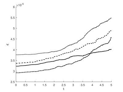
Figure 3: Averaged absolute errors of updating 1/3 of the parameters randomly per iteration from four different initial $\theta_{0}$ configurations.

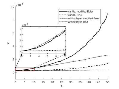
Figure 4: Averaged absolute errors of updating 1/3 of the parameters randomly per iteration. $``vanilla"$ represents random update in every time step; $``w/~{}first~{}layer"$ represents that the inclusion of the update parameters in the first layer is mandatory; $``modified~{}Euler"$ represents predictor-corrector (modified-Euler) method, and $``RK4"$ represents explicit fourth-order Runge-Kutta method.

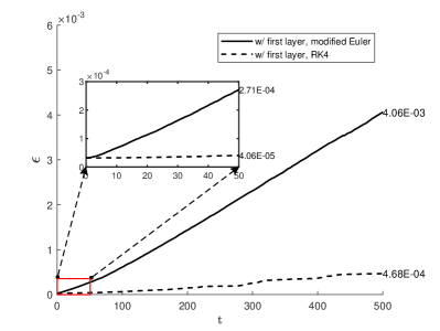
Figure 5: Averaged absolute errors of updating 1/3 of the parameters randomly per iteration. $``w/~{}first~{}layer"$ represents that the inclusion of the update parameters in the first layer is mandatory; $``modified~{}Euler"$ represents predictor-corrector (modified-Euler) method, and $``RK4"$ represents explicit fourth-order Runge-Kutta method.

3.2 The Navier-Stokes Equations

The incompressible Navier-Stokes (NS) equations are a set of nonlinear PDEs that describe the motion of fluid substances such as liquids and gases. The incompressible NS equations read as

$$\frac{\partial\mathbf{u}}{\partial t}+(\mathbf{u}\cdot\nabla)\mathbf{u} =-\nabla p+\nu\nabla^{2}\mathbf{u}+\mathbf{f},$$

$$\nabla\cdot\mathbf{u} =0,$$

where $\mathbf{u}=(u,v)$ denotes the velocity, $p$ is the pressure, $\mathbf{f}$ is the source term and $\nu$ is the viscosity. Here we consider the Taylor-Green vortex, an analytical expression of the NS equations:

$$u(x,y,t) =U_{0}\cos(x)\sin(y)e^{-2\nu t},$$

$$v(x,y,t) =-U_{0}\sin(x)\cos(y)e^{-2\nu t}$$

with $U_{0}=1,~{}\nu=1.$ The computational domain is $[-\pi,\pi]$. We assume that $u=\psi_{y},v=-\psi_{x}$ for some function $\psi(x,y,t)$, and we solve $\psi(x,y,t)$ in this experiment.

In this experiment, for the two sub-networks, we adopt $tanh$ activation and set two hidden layers with 30 neurons in each layer. Fig.6 shows the results of pETNNs with 200 parameters to update in each sub-network for solving the Taylor-Green vortex. The solution derived from the pETNNs (200) closely approximates the analytical solution, as evidenced by the error plots that show deviations on the order of $10^{-7}$, significantly surpassing the accuracy of the solution by the PINNs [20, 21]. Furthermore, we also compare the solutions obtained from the pETNNs with different ratios of updating parameters. Fig.7 demonstrates the results of updating 200, 400, 600 parameters in each sub-network and all parameters, which have similar absolute errors.

(a) Analytical solution, $\psi_{A}$

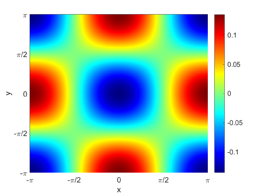
(b) Solution by pETNNs (200), $\psi_{p}$

(c) $\psi_{A}-\psi_{p}$

Figure 6: Profile of the solutions, $\psi$, to the Navier-Stokes equations at time $t=1$. The left (a) is the analytical solution denoted by $\psi_{A}$, the center (b) is the solution obtained by pETNNs (200 parameters to update randomly in each sub-network), denoted by $\psi_{p}$, and the right (c) depicts the discrepancy between the analytical solution and the numerical approximation, that is, $\psi_{A}-\psi_{p}$.

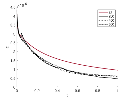
Figure 7: Absolute errors of the pETNNs with different subsets of parameters for solving the incompressible Navier-Stokes equations. There are 200, 400, 600 parameters in each sub-network and all of parameters to update.

3.3 High-dimensional Heat Equation

The heat equation is a fundamental PDE in the field of mathematics, physics, and engineering which describes the distribution of heat in a given region over time. It is a parabolic PDE and is the cornerstone of Fourier theory and heat conduction analysis. Here we consider the 10-dimensional heat equation,

$$\frac{\partial u}{\partial t}=v\Delta u,\quad x\in\Omega=[-1,1]^{10},v=1/\pi^{2},$$

with the initial values

$$u(x,t=0)=\prod_{i=1}^{10}\sin\left(\pi x_{i}\right),$$

and the Dirichlet boundary conditions, and its analytical solution is

$$u(x)=\prod_{i=1}^{10}\sin\left(\pi x_{i}\right)\exp(-dt).$$

In this experiment, each sub-network has three hidden layers with 30 neurons in each layer. The results obtained by pETNNs with different update parameters are plotted in Fig.8. We can see that they all have high accuracy, which demonstrate the efficacy of our pETNNs.

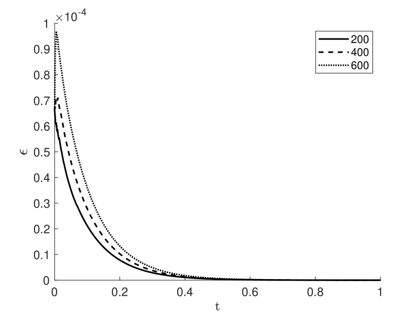
(a) Absolute error

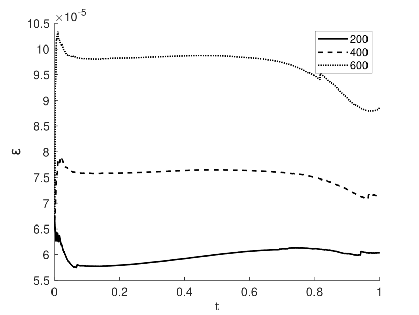
(b) Relative error

Figure 8: Absolute and Relative errors of pETNNs for solving 10D heat equation. Here 200, 400 and 600 parameters in each sub-network are updated randomly in every time step.

3.4 High-dimensional Transport Equation

We have used 2D and 3D transport equation to validate our pETNNs in the first experiment. Here we will adopt the pETNNs to solve the 10D transport equation to demonstrate the efficacy of our method for solving high-dimensional transport PDE. Here is the 10D transport equation,

$$\frac{\partial u}{\partial t}+c\sum_{i=1}^{d}\frac{\partial u}{\partial x_{i}}=0,\quad x\in\Omega=[-1,1]^{d}$$

with the initial values

$$u(x,t=0)=\prod_{i=1}^{d}\sin\left(\pi x_{i}\right),$$

and periodic boundary conditions. The analytical solutions are

$$u(x,t)=\prod_{i=1}^{d}\sin\left(\pi\left(x_{i}-ct\right)\right)$$

with $c=1$. We set that each sub-network consists of two hidden layers and each layer has 30 neurons. Fig.9 shows the results of employing Algorithm 2 to the 10D transport equation. The very small relative and absolute errors both demonstrate that our pETNNs perform well for solving high-dimensional transport equation. Additionally, we have also investigated the impact of parameter selection on numerical accuracy and stability. Within each sub-network, we fixed the update to 300 parameters. Various strategies were employed, including random update, mandatory update of the first layer’s parameters with each iteration, deliberately excluding the first layer’s parameters from update, and omitting bias from the updating process. The numerical results of these strategies are illustrated in Fig.10. The experimental results indicate that there is little difference in the precision of the results obtained by these update methods, which underscores the efficiency of Algorithm 2.

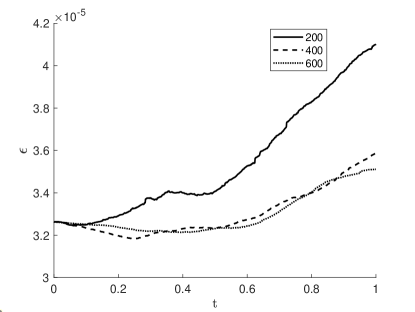
Figure 9: Absolute errors of pETNNs with randomized parameter update strategy for solving the 10D transport equation. Here 200, 400 and 600 parameters in each sub-network are updated randomly in every time step.

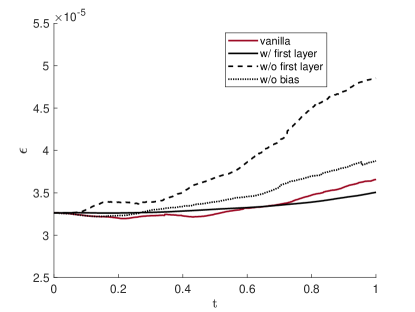
Figure 10: Absolute errors of pETNNs with 300 update parameters for solving the 10D transport equation. $``vanilla"$ denotes that the update parameters are randomly chosen in every time step; $``w/~{}first~{}layer"$ denotes that the inclusion of the update parameters in the first layer is mandatory, whereas $``w/o~{}first~{}layer"$ signifies precisely the opposite, indicating the exclusion; and $``w/o~{}bias"$ denotes the update parameters without the bias in every time step.

3.5 KdV-type Equation

In the last experiment, let us consider the KdV-type equation as follows:

$$\frac{\partial u}{\partial t}+c\sum_{i=1}^{d}\frac{\partial^{3}u}{\partial x_{i}^{3}}=f,\quad x\in\Omega=[-1,1]^{d},c=1/\pi^{3}.$$

The exact solution is

$$u(x,t)=\prod_{i=1}^{d}\sin\left(\pi x_{i}\right)\exp(-t)$$

with the corresponding source term

$$f=-\prod_{i=1}^{d}\sin(\pi x_{i})\exp(-t)-\sum_{i=1}^{d}\cos(\pi x_{i})\prod_{j=1,j\neq i}^{d}\sin(\pi x_{j})\exp(-t).$$

Here we choose $d=10,15$ and $20$, and for all cases, the sub-network has two hidden layers with 30 neurons in each layer. The absolute and relative errors are depicted in Figs. 11,12,13. All results show that our pETNNs show excellent performances for high-dimensional KdV-type equation with high accuracy.

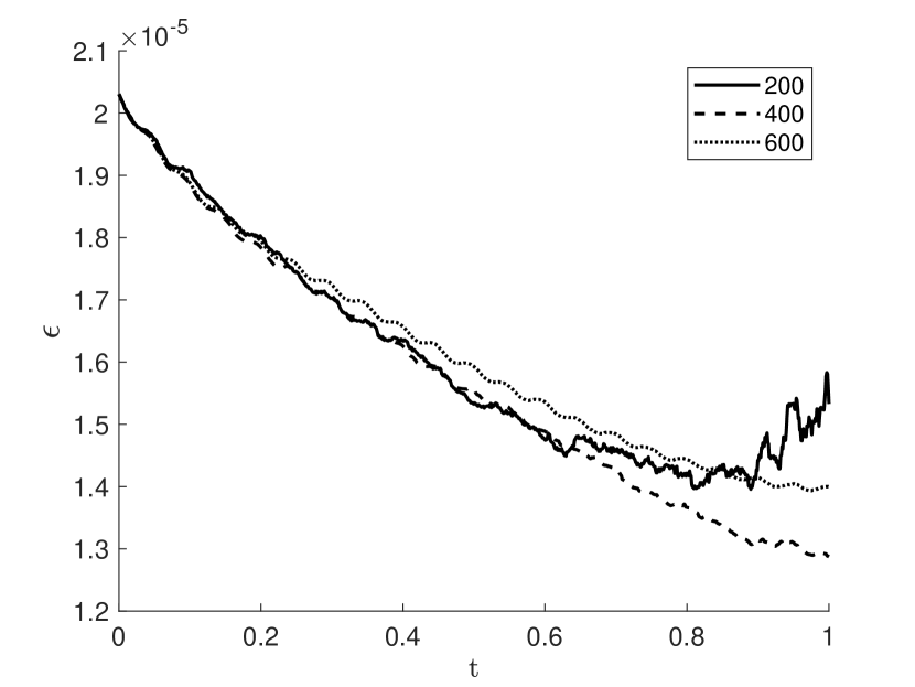
(a) Absolute error

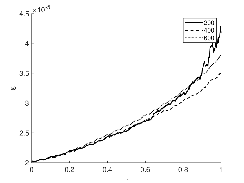
(b) Relative error

Figure 11: Absolute and relative errors of pETNNs for solving the 10D KdV-type equation. Here 200, 400 and 600 parameters in each sub-network are updated randomly in every time step.

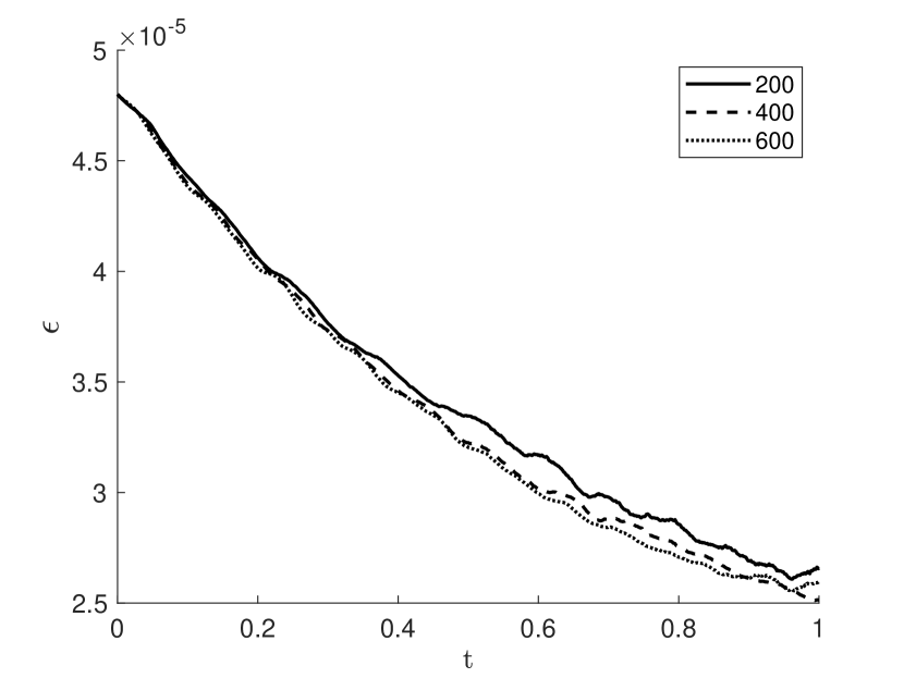
(a) Absolute error

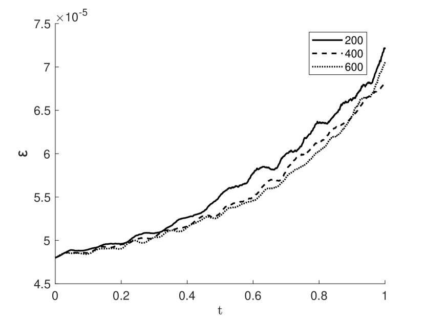
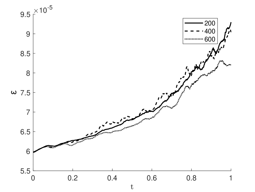
(b) Relative error

Figure 12: Absolute and relative errors of pETNNs for solving the 15D KdV-type equation. Here 200, 400 and 600 parameters in each sub-network are updated randomly in every time step.

(a) Absolute error

(b) Relative error

Figure 13: Absolute and relative errors of pETNNs for solving the 20D KdV-type equation. Here 200, 400 and 600 parameters in each sub-network are updated randomly in every time step.

4 Conclusions

This paper introduces the partial evolutionary tensor neural networks (pETNNs) framework as a groundbreaking solution for solving time-dependent partial differential equations (PDEs). The pETNNs blend the structural advantages of tensor neural networks (TNNs) with evolutionary parameters, yielding not only superior accuracy compared to conventional evolutional deep neural networks (EDNNs) but also exceptional extrapolation capabilities. By employing innovative strategies for parameter update, the proposed pETNNs can reduce computational cost significantly, and demonstrate their computational prowess in addressing high-dimensional time-dependent problems, expanding their utility beyond traditional applications. Numerical experiments conducted on various challenging equations, such as the incompressible Navier-Stokes equations, high-dimensional heat equation, and high-dimensional transport equation and Korteweg-de Vries type equation, highlight the superior performance of the pETNNs in accurately solving these complex problems. The findings indicate that the pETNNs make a noteworthy contribution to the field of computational methods for time-dependent equations and could play a significant role in advancing scientific research across various disciplines. On the other hand, although the implementation of pETNNs has demonstrated success, future research will aim to comprehensively investigate the scalability and applicability of the method. This investigation into scalability will include the adaptation of pETNNs to accommodate irregular boundary conditions, a systematic examination of parameter update methodologies, and an assessment of long-term stability. In terms of applicability, efforts will be directed towards employing this method to specific physical models, notably in addressing challenges raised in Bose-Einstein condensates [28], quasicrystals [29], liquid crystals [30], etc.

Code and Data Availability

Data and code are available from the corresponding author upon reasonable request for research purposes.

References

- [1] William Anderson and Mohammad Farazmand. Evolution of nonlinear reduced-order solutions for pdes with conserved quantities. SIAM Journal on Scientific Computing, 44(1):A176–A197, 2022.
- [2] Jules Berman and Benjamin Peherstorfer. Randomized sparse neural galerkin schemes for solving evolution equations with deep networks. In A. Oh, T. Neumann, A. Globerson, K. Saenko, M. Hardt, and S. Levine, editors, Advances in Neural Information Processing Systems, volume 36, pages 4097–4114. Curran Associates, Inc., 2023.
- [3] Joan Bruna, Benjamin Peherstorfer, and Eric Vanden-Eijnden. Neural galerkin schemes with active learning for high-dimensional evolution equations. Journal of Computational Physics, 496:112588, 2024.
- [4] Philippe G. Ciarlet. The Finite Element Method for Elliptic Problems. Classics in Applied Mathematics. Society for Industrial and Applied Mathematics, Philadelphia, PA, classics in applied mathematics edition, 2002.
- [5] George Cybenko. Approximation by superpositions of a sigmoidal function. Mathematics of Control, Signals and Systems, 2:303–314, 1989.
- [6] M. W. M. G. Dissanayake and N. Phan-Thien. Neural-network-based approximations for solving partial differential equations. Communications in Numerical Methods in Engineering, 10(3):195–201, 1994.
- [7] Yifan Du and Tamer A. Zaki. Evolutional deep neural network. Physical Review E, 104:045303, Oct 2021.
- [8] Weinan E and Bing Yu. The deep ritz method: A deep learning-based numerical algorithm for solving variational problems. Communications in Mathematics and Statistics, 6:1–12, 2018.
- [9] Zhiwei Gao, Liang Yan, and Tao Zhou. Failure-informed adaptive sampling for pinns. SIAM Journal on Scientific Computing, 45(4):A1971–A1994, 2023.
- [10] Kurt Hornik, Maxwell Stinchcombe, and Halbert White. Multilayer feedforward networks are universal approximators. Neural Networks, 2:359–366, 1989.
- [11] Ameya D. Jagtap, Kenji Kawaguchi, and George Em Karniadakis. Adaptive activation functions accelerate convergence in deep and physics-informed neural networks. Journal of Computational Physics, 404:109136, 2020.
- [12] Mariella Kast and Jan S Hesthaven. Positional embeddings for solving pdes with evolutional deep neural networks. arXiv e-prints, page arXiv: 2308.03461, 2023.
- [13] I.E. Lagaris, A. Likas, and D.I. Fotiadis. Artificial neural networks for solving ordinary and partial differential equations. IEEE Transactions on Neural Networks, 9(5):987–1000, 1998.
- [14] Randall J. LeVeque. Finite Difference Methods for Ordinary and Partial Differential Equations: Steady-State and Time-Dependent Problems. Society for Industrial and Applied Mathematics, Philadelphia, PA, 2007.
- [15] Yangfei Liao, Yifan Wang, and Hehu Xie. Solving high dimensional partial differential equations using tensor type discretization and optimization process. arXiv e-prints, page arXiv:2211.16548, 2022.
- [16] Zichao Long, Yiping Lu, and Bin Dong. PDE-Net 2.0: Learning PDEs from data with a numeric-symbolic hybrid deep network. Journal of Computational Physics, 399:108925, 2019.
- [17] Zichao Long, Yiping Lu, Xianzhong Ma, and Bin Dong. PDE-Net: Learning PDEs from data. In International Conference on Machine Learning, pages 3208–3216, 2018.
- [18] Lu Lu, Xuhui Meng, Zhiping Mao, and George Em Karniadakis. Deepxde: A deep learning library for solving differential equations. SIAM Review, 63(1):208–228, 2021.
- [19] Johannes Müller and Marius Zeinhofer. Achieving high accuracy with pinns via energy natural gradients. arXiv e-prints, page arXiv: 2302.13163, 2023.
- [20] Pi-Yueh Chuang and Lorena A. Barba. Experience report of physics-informed neural networks in fluid simulations: pitfalls and frustration. In Meghann Agarwal, Chris Calloway, Dillon Niederhut, and David Shupe, editors, Proceedings of the 21st Python in Science Conference, pages 28 – 36, 2022.
- [21] M. Raissi, P. Perdikaris, and G.E. Karniadakis. Physics-informed neural networks: A deep learning framework for solving forward and inverse problems involving nonlinear partial differential equations. Journal of Computational Physics, 378:686–707, 2019.
- [22] Jie Shen, Tao Tang, and Li-Lian Wang. Spectral Methods: Algorithms, Analysis and Applications, volume 41 of Springer Series in Computational Mathematics. Springer, Berlin, Heidelberg, 2011.
- [23] Justin Sirignano and Konstantinos Spiliopoulos. Dgm: A deep learning algorithm for solving partial differential equations. Journal of Computational Physics, 375:1339–1364, 2018.
- [24] Matthew Tancik, Pratul P. Srinivasan, Ben Mildenhall, Sara Fridovich-Keil, Nithin Raghavan, Utkarsh Singhal, Ravi Ramamoorthi, Jonathan T. Barron, and Ren Ng. Fourier Features Let Networks Learn High Frequency Functions in Low Dimensional Domains. Advances in Neural Information Processing Systems 33, pages 7537–7547, June 2020.
- [25] Chuwei Wang, Shanda Li, Di He, and Liwei Wang. Is physics informed loss always suitable for training physics informed neural network? In S. Koyejo, S. Mohamed, A. Agarwal, D. Belgrave, K. Cho, and A. Oh, editors, Advances in Neural Information Processing Systems, volume 35, pages 8278–8290. Curran Associates, Inc., 2022.
- [26] Yifan Wang, Pengzhan Jin, and Hehu Xie. Tensor neural network and its numerical integration. arXiv e-prints, page arXiv: 2207.02754, 2023.
- [27] Yifan Wang, Zhongshuo Lin, Yangfei Liao, Haochen Liu, and Hehu Xie. Solving high dimensional partial differential equations using tensor neural network and a posteriori error estimators. arXiv e-prints, page arXiv:2311.02732, 2023.
- [28] Jianyuan Yin, Zhen Huang, Yongyong Cai, Qiang Du, and Lei Zhang. Revealing excited states of rotational bose-einstein condensates. The Innovation, 5(1), 2024.
- [29] Jianyuan Yin, Kai Jiang, An-Chang Shi, Pingwen Zhang, and Lei Zhang. Transition pathways connecting crystals and quasicrystals. Proceedings of the National Academy of Sciences, 118(49):e2106230118, 2021.
- [30] Jianyuan Yin, Yiwei Wang, Jeff Z. Y. Chen, Pingwen Zhang, and Lei Zhang. Construction of a pathway map on a complicated energy landscape. Phys. Rev. Lett., 124:090601, Mar 2020.