FrameQuant: Flexible Low-Bit Quantization for Transformers

Abstract

Transformers are the backbone of powerful foundation models for many Vision and Natural Language Processing tasks. But their compute and memory/storage footprint is large, and so, serving such models is expensive often requiring high-end hardware. To mitigate this difficulty, Post-Training Quantization seeks to modify a pre-trained model and quantize it to eight bits or lower, significantly boosting compute/memory/latency efficiency. Such models have been successfully quantized to four bits with some performance loss. In this work, we outline a simple scheme to quantize Transformer-based models to just two bits (plus some overhead) with only a small drop in accuracy. Key to our formulation is a concept borrowed from Harmonic analysis called Fusion Frames. Our main finding is that the quantization must take place not in the original weight space, but instead in the Fusion Frame representations. If quantization is interpreted as the addition of noise, our casting of the problem allows invoking an extensive body of known consistent recovery and noise robustness guarantees. Further, if desired, de-noising filters are known in closed form. We show empirically, via a variety of experiments, that (almost) two-bit quantization for Transformer models promises sizable efficiency gains.

1 Introduction

Transformer-based Large Language Models (LLMs) dominate the landscape for Natural Language Processing tasks such as language translation and text summarization Zhang et al. (2023); Touvron et al. (2023); Zhang et al. (2022a). Vision Transformers (VITs) adapt this idea for computer vision, and achieve state-of-the-art results on image classification Zhai et al. (2022), object detection Zhang et al. (2022b), generation Chang et al. (2022); Hudson and Zitnick (2021) and segmentation Cheng et al. (2022); Ranftl et al. (2021). There is general agreement that scale provides remarkable new capabilities.

While large models offer strong performance improvements, their deployment as a module within a product creates unique challenges. For example, serving these models on expensive hardware can drastically increase data center costs. Even loading these models on consumer-grade machines is difficult, and the ability to handle heterogeneous resource-constrained devices is almost infeasible. This has led to various efficiency-focused strategies for model compression including but not limited to distillation Hinton et al. (2015); Zhu et al. (2021), pruning Chen and Zhao (2019), sparsity Yu et al. (2012); Yun et al. (2020) and quantization Han et al. (2016); Banner et al. (2019). Among these methods, Post-Training Quantization offers unique advantages in that it does not change the model architecture or training scheme.

This paper presents a new Post-Training Quantization scheme, FrameQuant, that offers much more flexibility to strike a balance between reducing model size and preserving model quality. Specifically, FrameQuant offers what may be considered equivalent to using a fractional number of bits for quantization, e.g., 2.1 or 2.2 bits: this is valuable because for large Transformer-based models like GPT, model quality deteriorates fast Frantar et al. (2023) as we reduce bit width in the low-bit quantization regime (e.g., 2-bit). Further, depending on the accuracy needs of the downstream task at hand or a desire to control the worst-off error, more flexibility offers the user more control. Towards this goal, our main idea is to compute a specific type of redundant/over-complete representation of a pre-trained weight matrix and quantize the matrix in that representation. We will see how robustness to quantization error will follow naturally from our choice of representation. The de-quantization step uses a straightforward scheme to re-construct the full-precision weights. We leverage a mature concept from Harmonic analysis, Fusion Frames, as the foundation for our proposal.

Fusion Frames Donoho et al. (1998); Christensen (2018) serve an important role in signal processing in analog-to-digital conversion and signal transmission. Frames are guaranteed to be robust when the Frame coefficients are corrupted by additive noise. They are very numerically stable, and if additional compute/memory overhead is acceptable, denoising filters with good theoretical properties or provably optimal recovery schemes are known. To our knowledge, Frame theory for neural network quantization is unexplored. Our key contributions include (a) an approach that offers fractional bit quantization capabilities with theoretical guarantees. (b) We empirically verify that Transformer-based models can be quantized to two bits (or 2.x bits), on an extensive basket of 15 popular Vision Transformers and Large Language Models from the OPT Zhang et al. (2022a) as well as Llama2 Touvron et al. (2023) classes. We achieve consistent improvements over all existing baselines.

1.1 Related Work

Given the growth in the scale of foundation models common in our community, model compression is an active topic of research. Distillation Hinton et al. (2015); Zhu et al. (2021), pruning/shrinking Chen and Zhao (2019) and the use of sparsity is quite common Yu et al. (2012); Yun et al. (2020). There is growing interest Rokh et al. (2023); Gholami et al. (2022) in approaches that perform model compression via quantization either (i) during training or (ii) post-training since minimal changes to the architecture are needed. Quantization during training works well Gholami et al. (2022); Nagel et al. (2021), but models must be re-trained. Post-training quantization (PTQ) methods Nagel et al. (2019) simply quantize a pre-trained model on a small calibration set, and involve much less work. These methods are effective for large language models like OPT Zhang et al. (2022a), BLOOM Scao et al. (2023) and can reduce the bit-width with only a small degradation in performance. For example, Nagel et al. (2020) analyzed the effect of data-dependent rounding. A layer-wise proxy loss was studied and AdaRound quantization was proposed to efficiently minimize this loss. The approach in Frantar and Alistarh (2022) minimizes the squared error similar to Nagel et al. (2020), but quantizes each layer individually while adjusting the remaining unquantized weights using the Hessian of the proxy loss term following Lecun et al. (1989); Hassibi et al. (1993). OPTQ Frantar et al. (2023)(formerly GPTQ) extended upon the ideas in OBQ Frantar and Alistarh (2022), and offered other adjustments that yielded a stable scheme that could compress large language models like OPT-175B or BLOOM-176B to 3 or 4 bits per parameter without a large loss in accuracy. For Vision Transformers, PTQ4ViT Yuan et al. (2022) quantifies the weights in two stages, and uses a Hessian-guided search for the optimal scale for the weights. In Liu et al. (2021a), a feature map is used to search for the optimal quantization interval for maintaining similarity between the quantized and original feature maps. The method also chooses different bit widths for each layer. Other strategies proposed for PTQ include Ding et al. (2022); Li et al. (2023). We note a recent concurrent result for two-bit quantization for language models reported in Chee et al. (2023). Our approaches are based on different starting points: our choice of Frame theory to minimize quantization error versus the choice in Chee et al. (2023) of using incoherence as a pre and post-processing step, which is later shown to offer desirable theoretical properties. But fundamentally, both methods work well due to similar underlying principles related to basis expansions (on a space-filling basis). We discuss later how Chee et al. (2023) can be viewed as a special version of our formulation (but with no redundancy).

2 Finite Frame Theory and Fusion Frames

Frames generalize the Orthogonal basis decomposition of a Hilbert space and provide redundant representations. Finite frames find applications in robust signal transmission with quantization and erasures Goyal et al. (1998, 2001); Casazza and Kovačević (2003), Coding theory Strohmer and Heath Jr (2003), distributed processing Casazza et al. (2008), Compressed Sensing Boufounos et al. (2009) among others. We start with a brief review of relevant concepts. Readers familiar with these concepts may skim this section.

Consider a finite-dimensional Hilbert space $\mathcal{H}$ of dimension $d$. Throughout the paper, we denote this space as $\mathcal{H}^{d}$.

Definition 2.1 (Frames).

A family of $k$ vectors $\upphi=(\varphi_{i})_{i=1}^{k}$ in $\mathcal{H}^{d}$ is called a frame for $\mathcal{H}^{d}$ if there exist constants $0<A\leq B<\infty$ such that

$$A||x||^{2}\leq\sum_{i=1}^{k}|\langle x,{\color[rgb]{0.1,0.0499999999999999,0.96}\varphi_{i}}\rangle|^{2}\leq B||x||^{2}$$ (1)

for all $x\in\mathcal{H}^{d}$ where $\langle\cdot,\cdot\rangle$ is the dot-product. The constants $A$ and $B$ are the lower and upper frame bounds.

Figure 1: Examples of Tight Frames examples $\mathbb{R}^{2}$ for $k=4,5,\dots$ 11

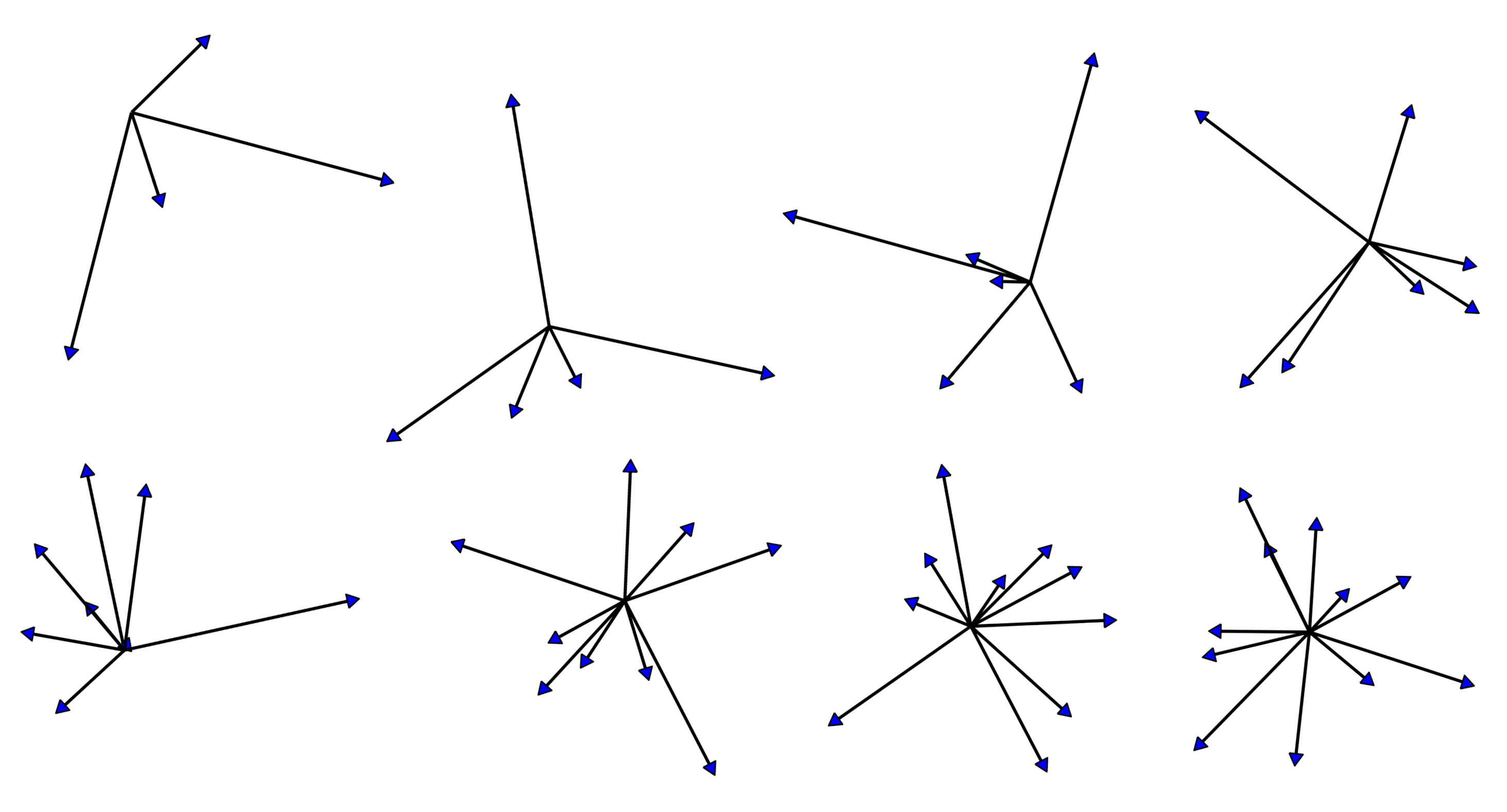
If $A$ and $B$ are not too large, the sandwich expression suggests that $x$ will not be poorly distorted when we calculate its inner products with a frame. When $A=B$, $\upphi$ is called a A-tight frame. When $A=B=1$, we get a Parseval’s frame. Fig. 1 shows examples of Tight Frames for $\mathbb{R}^{2}$ for different $k$’s. The lower bound is equivalent to asking that $\upphi$ span $\mathcal{H}$. So, for a frame, we always have $k\geq d$. If $k=3d$, the redundancy is $r=3$.

Fusion Frames provide a way for fusing “smaller” frames to construct large frames, offering various efficiency and robustness properties Eldar and Michaeli (2008). Formally,

Definition 2.2 (Fusion Frames).

Let ${\color[rgb]{0,0,1}(\mathcal{W}_{i})}_{i=1}^{k}$ be a family of subspaces in $\mathcal{H}^{d}$, and let $(w_{i})_{i=1}^{k}\subseteq\mathbb{R}^{+}$ be a family of weights. Then, $({\color[rgb]{0,0,1}(\mathcal{W}_{i},w_{i})})_{i=1}^{k}$ is a fusion frame for $\mathcal{H}^{d}$, if there exists constants $0<A\leq B<\infty$ such that

$$A||x||^{2}\leq\sum_{i=1}^{k}w_{i}^{2}||U_{i}(x)||^{2}\leq B||x||^{2}\quad\text{for all }x\in\mathcal{H}^{d}$$

where ${\color[rgb]{0,1,1}U_{i}}$ denotes the orthonormal projection onto the subspace ${\color[rgb]{0,0,1}\mathcal{W}_{i}}$ for each $i$. The constants $A$ and $B$ still denote the lower and upper fusion frame bounds respectively.

Similar to the Frames case, the Fusion Frame $({\color[rgb]{0,0,1}(\mathcal{W}_{i},w_{i})})_{i=1}^{k}$ is referred to as a tight fusion frame if $A=B$ and as a Parseval fusion frame if $A=B=1$. Finally, if $w_{i}=1$ for all $i$, we simply utilize the notation ${\color[rgb]{0,0,1}(\mathcal{W}_{i})}_{i=1}^{k}$.

2.1 Operators in Fusion Frames

Fusion Frame (FF) operators can be formally defined using Hilbert direct sum. Since we use the operators for model quantization, without loss of generality, we describe them in terms of vectors and matrices, to keep notations simple. Let $({\color[rgb]{0,0,1}(\mathcal{W}_{i},w_{i})})_{i=1}^{k}$ be a Fusion Frame for $\mathcal{H}^{d}$ with orthonormal basis ${\color[rgb]{0.1,0.0499999999999999,0.96}(P_{i})}_{i=1}^{k}$ respectively.

The Analysis operator $\mathcal{T}_{\mathcal{W}}$ takes a signal $x\in\mathcal{H}^{d}$ and computes its dot product with all the basis ${\color[rgb]{0.1,0.0499999999999999,0.96}(P_{i})}_{i=1}^{k}$. The results represent $x$ w.r.t. the FF as

$$\mathcal{T}_{\mathcal{W}}:x\mapsto(w_{i}{\color[rgb]{0,1,0}P_{i}^{T}(x)})_{i=1}^{k}$$ (2)

The Synthesis operator $\mathcal{T}^{*}_{\mathcal{W}}$ is the adjoint of the analysis operator, and takes a sequence of representation vectors ${\color[rgb]{0,1,0}{(y_{i})}_{i=1}^{k}}$ and outputs a signal in $\mathcal{H}^{d}$: the reconstruction of the original signal from its FF representation defined as

$$\mathcal{T}^{*}_{\mathcal{W}}:{\color[rgb]{0,1,0}(y_{i})}_{i=1}^{k}\mapsto\sum_{i=1}^{k}w_{i}{\color[rgb]{0.1,0.0499999999999999,0.96}P_{i}}({\color[rgb]{0,1,0}y_{i}})$$ (3)

The Fusion Frame operator $\mathcal{S}_{\mathcal{W}}$ is defined as the composition of these two operators. It first computes the FF representation of a signal in $\mathcal{H}^{d}$ in different subspaces using the Analysis operator. Then, when needed, we can reconstruct the signal back from these representations using the Synthesis operator. When the Fusion Frame is tight, the reconstruction is exact Casazza et al. (2011). Formally,

$$\mathcal{S}_{\mathcal{W}}=\mathcal{T}^{*}_{\mathcal{W}}\mathcal{T}_{\mathcal{W}}:x\mapsto\sum_{i=1}^{k}w_{i}^{2}{\color[rgb]{0,1,1}U_{i}(x)}$$ (4)

Here, ${\color[rgb]{0,1,1}U_{i}}={\color[rgb]{0.1,0.0499999999999999,0.96}P_{i}}{\color[rgb]{0.1,0.0499999999999999,0.96}P_{i}}^{T}$ is the orthogonal projection onto the subspace ${\color[rgb]{0,0,1}\mathcal{W}_{i}}$. If the Fusion Frame is tight, we have $\mathcal{S}_{\mathcal{W}}=AI_{d}$ where $I_{d}$ is the $d\times d$ Identity Matrix. Throughout, we will use Parseval Fusion Frames, where the frame bounds $A=B=1$. Fusion Frames offer many other properties but due to space, we will keep the presentation focused.

How will Fusion Frames be used? An easy way to see Fusion Frames in practice is to work out a simple example,

Example 1.

Consider the Euclidean space $\mathcal{H}^{d}=\mathbb{R}^{4}$. Say, an oracle gives us a Fusion Frame where we have $k=3$ subspaces, and each subspace is of equal dimension $\rho=2$. For notational ease, we represent these subspaces with their Synthesis operator $\mathcal{T}^{*}_{\mathcal{W}}$

$$=\left({\color[rgb]{0.1,0.0499999999999999,0.96}\begin{bmatrix}0.57&0.00\\ 0.00&0.57\\ 0.57&0.00\\ 0.00&0.57\end{bmatrix},}{\color[rgb]{0.1,0.0499999999999999,0.96}\begin{bmatrix}0.57&0.00\\ 0.00&0.57\\ -0.28&0.50\\ -0.50&-0.28\end{bmatrix},}{\color[rgb]{0.1,0.0499999999999999,0.96}\begin{bmatrix}0.57&0.00\\ 0.00&0.57\\ -0.28&-0.50\\ 0.50&-0.28\end{bmatrix}}\right)$$

We want to compute the FF representation of a signal $x=\begin{bmatrix}-1&-0.5&0.5&1\end{bmatrix}^{T}$. To do so, we must apply the Analysis operator $\mathcal{T}_{\mathcal{W}}$ on $x$. The Analysis operator is simply based on the individual transposes in $\mathcal{T}^{*}_{\mathcal{W}}$ defined above.

$${\color[rgb]{0.1,0.0499999999999999,0.96}\begin{bmatrix}0.57&0.00&0.57&0.00\\ 0.00&0.57&0.00&0.57\end{bmatrix},}{\color[rgb]{0.1,0.0499999999999999,0.96}\begin{bmatrix}0.57&0.00&-0.28&-0.50\\ 0.00&0.57&0.50&-0.28\end{bmatrix}}\cdots$$

Applying $\mathcal{T}_{\mathcal{W}}$ on $x$, we get the FF representations

$${\color[rgb]{0,1,0}\mathcal{T}_{\mathcal{W}}(x)}=\left({\color[rgb]{0,1,0}\begin{bmatrix}-0.28\\ 0.28\end{bmatrix},}{\color[rgb]{0,1,0}\begin{bmatrix}-1.22\\ -0.32\end{bmatrix},}{\color[rgb]{0,1,0}\begin{bmatrix}-0.22\\ -0.82\end{bmatrix}}\right)$$

To get the actual projections of $x$ onto different subspaces ${\color[rgb]{0,0,1}\mathcal{W}_{i}}$, we multiply these coefficients with the scaled orthonormal basis $(w_{i}{\color[rgb]{0.1,0.0499999999999999,0.96}P_{i}})_{i=1}^{k}$ of their corresponding subspaces

$$(w_{i}^{2}{\color[rgb]{0,1,1}U_{i}(x)})_{i=1}^{3}=\left({\color[rgb]{0,1,1}\begin{bmatrix}-0.1667\\ 0.1667\\ -0.1667\\ 0.1667\end{bmatrix}},{\color[rgb]{0,1,1}\begin{bmatrix}-0.7053\\ -0.1890\\ 0.1890\\ 0.7053\end{bmatrix}},{\color[rgb]{0,1,1}\begin{bmatrix}-0.1280\\ -0.4777\\ 0.4777\\ 0.1280\end{bmatrix}}\right)$$

We can verify by checking the identity $\mathcal{S}_{\mathcal{W}}=I_{d}$ or checking that $\sum_{i=1}^{3}w_{i}^{2}{\color[rgb]{0,1,1}U_{i}(x)}=x$ that this Fusion Frame is a Parseval’s frame. Applying the Synthesis operator $\mathcal{T}^{*}_{\mathcal{W}}$ on the projections above recovers $x$ perfectly.

Corrupting FF representations by noise. What happens when the Fusion frame representations are corrupted by noise, say due to erasure or quantization? Because of redundancy in the representation of a signal, we expect some immunity to corruptions in the representations due to noise. In the current example, this is indeed the case. If we add noise to $\mathcal{T}_{\mathcal{W}}(x)$ with an SNR of $10$dB and use the noisy coefficients to reconstruct $x$ back, we observe an MSE reduction of $33\%$ at a redundancy factor of $r=1.5\times$ and $50\%$ MSE reduction $r=2\times$, consistent with theory Goyal et al. (1998).

Quantizing Transformer layers. Let us consider quantizing each layer in a Transformer model as in Nagel et al. (2020); Frantar and Alistarh (2022); Frantar et al. (2023); Yuan et al. (2022), e.g., by quantizing individual weights or columns, one by one. First, notice that the quantization error/noise is weight-dependent. Further, the error will also depend on how all other weights are quantized. The only way to guide a quantization scheme is the evaluation of a loss (to be described shortly) on a small calibration dataset $\mathcal{D}$. In this regime, even with strong assumptions on the noise, it is difficult to say much about the quality of the de-quantization. On the other hand, far more is known Goyal et al. (1998); Waldron (2019); Casazza and Kutyniok (2012) about the behavior of quantization of data given in an appropriate Frame basis (e.g., Fusion Frames), and error bounds on the reconstruction are available. Put simply, quantization noise in the space of Frame projections incurs far less error in the reconstructions due to the robustness of Frame representations. §3 will leverage this principle.

2.2 Tight Fusion Frames and their construction

We first define the type of Fusion Frames we will use and then describe how they can be constructed.

Definition 2.3 (Tight Fusion Frames or TFF).

For $A>0$ and with $I_{d}$ giving the $d\times d$ Identity matrix, a $(k,\rho,d)$-TFF is a sequence $\{{\color[rgb]{0,1,1}U_{i}}\}_{i=1}^{k}$ of $d\times d$ orthogonal projection matrices of rank $\rho$ and scalars $\{w_{i}\}_{i=1}^{k},w_{i}>0$ such that

$$\sum_{i=1}^{k}w_{i}^{2}{\color[rgb]{0,1,1}U_{i}}=AI_{d}.\vspace{-10pt}$$ (5)

A $(k,\rho,d)$-TFF is a sequence of $k$ equidimensional sub-spaces of dimension $\rho$ in a $d$-dimensional space, and ${\color[rgb]{0,1,1}U_{i}}$ is the orthogonal projection matrix onto the $i^{th}$ sub-space.

Constructing TFFs. The algorithm in Casazza et al. (2011) can be used to generate TFFs if we provide the dimension $d$, the number $k$ of subspaces we need, and the dimension $\rho$ of each of these subspaces. The algorithm has two main steps. First, one generates a Tight Frame of $d$ unit norm vectors for the complex domain $\mathbb{C}^{\rho}$. Then, this Frame is modulated with the square roots of unity to generate the $k$ subspaces for $\mathbb{C}^{d}$. We use a simple construction described in Fickus et al. (2023) to extend these Fusion Frames to $\mathbb{R}^{d}$. Since it can be used as a black-box module, we skip the details and include a brief synopsis in Appendix §I.

Remarks. A few properties are useful to note. This Fusion Frame construction is sparse/block diagonal and can be generated one sub-space at a time. To generate another Fusion Frame, we can hit it with a random rotation. Depending on the Transformer model at hand, the dimension of the activations of the layer determines $d$. For a desired redundancy factor ($k\times\rho\geq d$) in our frames, given $d$ we simply choose a $k$ and $\rho$ such that they are valid (i.e., a TFF exists for the triple $(k,\rho,d)$) according to Casazza et al. (2011). If not, we simply use a slightly lower redundancy factor $r$ knowing that we will always have a trivial solution for $k=1$ and $\rho=d$.

3 Fusion Frames based Quantization

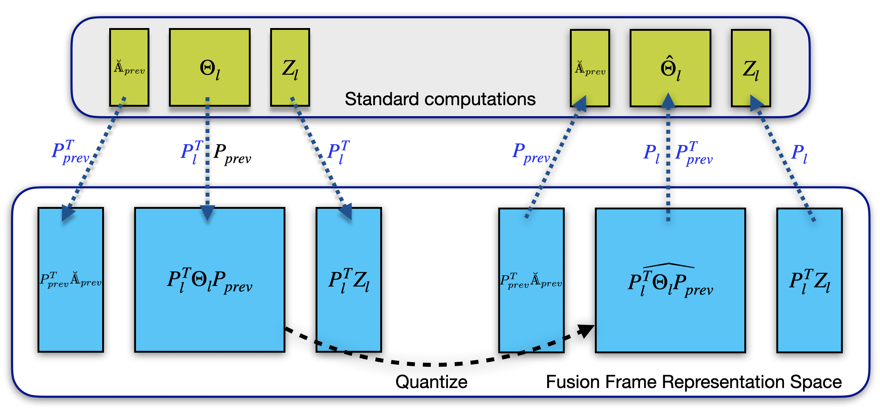
We can now leverage the ideas described in the preceding sections for quantizing the parameters of a Transformer model. Consistent with common PTQ approaches Nagel et al. (2020); Frantar and Alistarh (2022); Frantar et al. (2023); Yuan et al. (2022), we perform quantization layer-by-layer, minimizing the proxy loss between the quantized and non-quantized output of the layer. Fig. 2 gives a graphical view of our algorithm.

Figure 2: Illustration of standard calculation (on top) versus the corresponding calculations in FF space (bottom)

What are analogous calculations in FF space? Consider a layer $l$ in a Transformer model, with parameters $\Theta_{l}$. Let ${\breve{\mathds{A}}}_{\rm prev}$ be the activation of the already quantized previous layer for the examples in the calibration set $\mathcal{D}$. The (non-quantized) output $Z_{l}$ of layer $l$ is

$${Z}_{l}=\Theta_{l}{\breve{\mathds{A}}}_{\rm prev}$$ (6)

Here, $\Theta_{l}$ maps the input ${\breve{\mathds{A}}}_{\rm prev}$ to the output $Z_{l}$. To avoid directly quantizing $\Theta_{l}$, we want the quantization noise to instead impact the analogous terms in the Fusion Frame representation (but equivalent calculation as (6)). To this end, let us set up some notations. In general, the dimension of $Z_{l}$ and ${\breve{\mathds{A}}}_{\rm prev}$ may not be the same. So, the number of subspaces in their respective Fusion Frames will be different. Let $k,k_{\rm prev}$ denote the number of subspaces for $Z_{l}$ and ${\breve{\mathds{A}}}_{\rm prev}$ respectively. In other words, ${\color[rgb]{0,0,1}\mathcal{W}^{l}}={\color[rgb]{0,0,1}(\mathcal{W}_{i}^{l})}_{i=1}^{k}$ and ${\color[rgb]{0,0,1}\mathcal{W}^{\rm prev}}={\color[rgb]{0,0,1}(\mathcal{W}_{i}^{\rm prev})}_{i=1}^{k_{\rm prev}}$. Let the sequence of orthonormal basis for the subspaces of ${\color[rgb]{0,0,1}\mathcal{W}^{l}}$ and ${\color[rgb]{0,0,1}\mathcal{W}^{\rm prev}}$ be given by ${\color[rgb]{0.1,0.0499999999999999,0.96}(P_{i}^{l})}_{i=1}^{k}$ and ${\color[rgb]{0.1,0.0499999999999999,0.96}(P_{i}^{\rm prev})}_{i=1}^{k_{\rm prev}}$ respectively. To reduce notational clutter, we absorb the scalars $w_{i}$ into ${\color[rgb]{0.1,0.0499999999999999,0.96}P_{i}}$. To write down the expression in FF space, for simplicity, let us vectorize the set of orthogonal basis above and define

$${\color[rgb]{0.1,0.0499999999999999,0.96}P_{l}}=[{\color[rgb]{0.1,0.0499999999999999,0.96}P^{l}_{1}}{\color[rgb]{0.1,0.0499999999999999,0.96}P^{l}_{2}\dots P^{l}_{k}}]\;\text{and}\;{\color[rgb]{0.1,0.0499999999999999,0.96}P_{\rm prev}}=[{\color[rgb]{0.1,0.0499999999999999,0.96}P^{\rm prev}_{1}P^{\rm prev}_{2}\dots P^{\rm prev}_{k_{\rm prev}}}]$$

Taking the FF representations of the output $Z_{l}$ means

$${\color[rgb]{0,1,0}P_{l}^{T}Z_{l}}={\color[rgb]{0.1,0.0499999999999999,0.96}P_{l}^{T}}\underbrace{\Theta_{l}{\breve{\mathds{A}}}_{\rm prev}}_{=Z_{l}}$$ (7)

Rearranging brackets,

$${\color[rgb]{0.1,0.0499999999999999,0.96}P_{l}^{T}}\Theta_{l}{\breve{\mathds{A}}}_{\rm prev} ={\color[rgb]{0.1,0.0499999999999999,0.96}P_{l}^{T}}\Theta_{l}({\color[rgb]{0.1,0.0499999999999999,0.96}P_{\rm prev}P_{\rm prev}^{T}}){\breve{\mathds{A}}}_{\rm prev}$$ (8)

$$=({\color[rgb]{0.1,0.0499999999999999,0.96}P_{l}^{T}}\Theta_{l}{\color[rgb]{0.1,0.0499999999999999,0.96}P_{\rm prev}})({\color[rgb]{0,1,0}P_{\rm prev}^{T}{\breve{\mathds{A}}}_{\rm prev}})$$ (9)

In the above expression, the object $({\color[rgb]{0.1,0.0499999999999999,0.96}P_{l}^{T}}\Theta_{l}{\color[rgb]{0.1,0.0499999999999999,0.96}P_{\rm prev}})$ maps the FF representation of $\breve{\mathds{A}}_{\rm prev}$, i.e., $({\color[rgb]{0,1,0}P_{\rm prev}^{T}{\breve{\mathds{A}}}_{\rm prev}})$, to the FF representation of $({\color[rgb]{0,1,0}P_{l}^{T}Z_{l}})$. This operation is completely in the FF representation space as desired.

A notation simplification allows us to cross-reference what our FF-space calculations are doing w.r.t. the objective function. Let ${\color[rgb]{0,1,0}C_{\rm prev}}={\color[rgb]{0,1,0}P_{\rm prev}^{T}{\breve{\mathds{A}}}_{prev}}$ and $D_{l}={\color[rgb]{0.1,0.0499999999999999,0.96}P_{l}^{T}}\Theta_{l}{\color[rgb]{0.1,0.0499999999999999,0.96}P_{\rm prev}}$. Our objective is to quantize $D_{l}$ to $\hat{D}_{l}$ while minimizing the proxy loss in terms of FF representations,

$$\mathcal{L}(\hat{D}_{l}) =||D_{l}{\color[rgb]{0,1,0}C_{\rm prev}}-\hat{D}_{l}{\color[rgb]{0,1,0}C_{\rm prev}}||_{F}^{2}$$

$$=\text{tr}((D_{l}-\hat{D}_{l})^{T}{\color[rgb]{0,1,0}C_{\rm prev}^{T}C_{\rm prev}}(D_{l}-\hat{D}_{l}))$$

$$=\text{tr}((D_{l}-\hat{D}_{l}){\color[rgb]{0,1,0}C_{\rm prev}C_{\rm prev}^{T}}(D_{l}-\hat{D}_{l})^{T})$$

The term $\tilde{H}={\color[rgb]{0,1,0}C_{\rm prev}C_{\rm prev}^{T}}$ corresponds to the Hessian prominent in most published results on PTQ strategies Nagel et al. (2020); Frantar and Alistarh (2022); Frantar et al. (2023); Chee et al. (2023). So, our loss is the same as others, except that we are operating in the FF representation space and enjoy all the associated noise robustness properties. Further, because the loss for quantizing the transformed weights $D_{l}$ is the same as e.g., Frantar et al. (2023), we can directly use the Hessian-based iterative quantization algorithms in Frantar and Alistarh (2022); Frantar et al. (2023) with minimal changes. Finally, following recent results in Post-training Quantization Nagel et al. (2020); Frantar and Alistarh (2022); Frantar et al. (2023); Chee et al. (2023) and to facilitate fair comparisons, we only quantize the transformed weights $(D_{l})$ while leaving the activation projections ${\color[rgb]{0,1,0}C_{\rm prev}}$ unchanged, noting that successful activation quantization has also been reported separately for up to four bits Ding et al. (2022); Yuan et al. (2022).

0:  Weight matrix $\Theta_{l}$, previous layer activations ${\breve{\mathds{A}}}_{prev}$, input and output Fusion Frames ${\color[rgb]{0.1,0.0499999999999999,0.96}P_{l}},{\color[rgb]{0.1,0.0499999999999999,0.96}P_{\rm prev}}$, block size $B$

  1: Compute ${\color[rgb]{0,1,0}C_{\rm prev}}={\color[rgb]{0,1,0}P_{\rm prev}^{T}A_{\rm prev}}$, $D_{l}={\color[rgb]{0.1,0.0499999999999999,0.96}P_{l}^{T}}\Theta_{l}{\color[rgb]{0.1,0.0499999999999999,0.96}P_{\rm prev}}$

  2: Compute $\sigma=std(D_{l}),\;\;\;\mu=mean(D_{l})$

  3: $D_{l}=2\sigma\text{ clip}(D_{l},\mu-2\sigma,\mu+2\sigma)$

  4: $\hat{D}_{l}=quantize(D_{l},{\color[rgb]{0,1,0}C_{\rm prev}},B)$  // modified GPTQ

  5: Store $\hat{D}_{l}$      // store the quantized matrix $\hat{D}_{l}$

  return ${\color[rgb]{0.1,0.0499999999999999,0.96}P_{l}}\hat{D}_{l}{\color[rgb]{0,1,0}C_{\rm prev}}$  // return quantized layer activations

Algorithm 1 FrameQuant

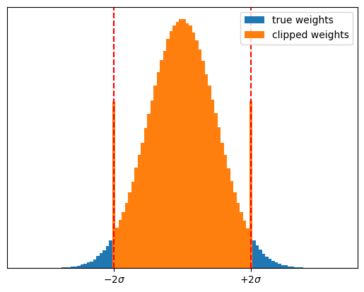
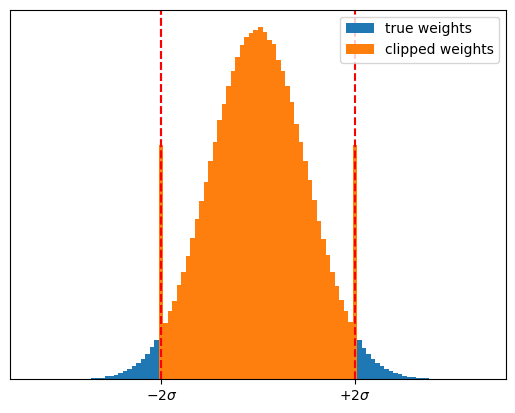
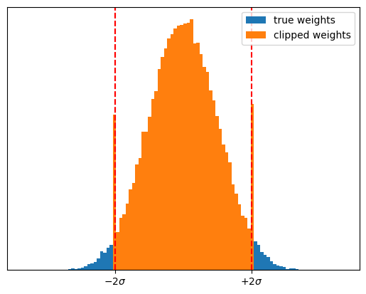
Details of the quantization procedure. Other than working in the FF space, the quantization itself is almost identical to Frantar et al. (2023). We use the iterative method from Frantar et al. (2023) with some modifications to improve the stability of our algorithm. For example, we found that clipping the weights before calling the iterative scheme from GPTQ reduces the weight range during quantization. This effectively adds more quantization noise to the outlier weights that are too large. Since Fusion Frames spread out the energy uniformly among different subspaces, we observe that there are only a few outliers in the transformed Weight matrices, and hence clipping them boosts performance. We found that simply clipping the weights at $2\sigma$ (assuming a Normal distribution), where $\sigma$ is the standard deviation of $D_{l}$, works well in practice. We observe that this change also helps the method in Chee et al. (2023) (and this modified algorithm is also included in our baselines). Alg. 1 shows the sequence of steps in FrameQuant.

3.1 Robustness of Fusion Frames

We now state some technical results that apply to both Frames and Fusion Frames.

1. Redundancy related guarantees. During quantization, the Fusion Frame coefficients are corrupted. This can be modeled as an additive noise being added to these coefficients. Assume that the redundancy factor is $r>1$. Even with classical analysis, the result in Rozell and Johnson (2005); Goyal et al. (1998) shows that when using Tight Frames to reconstruct the signal from noisy coefficients, for memoryless quantization, we get an MSE reduction of $\mathcal{O}(1/r)$. A rate of $\mathcal{O}(1/r^{2})$ for consistent reconstruction can also be achieved by solving an LP during the dequantization step Goyal et al. (1998). While this may not be preferred in practice, we know that if adopted, this matches the lower bound of $(1/r^{2})$, see Ch. 2 in Goyal et al. (1998).

2. Another benefit of Frame representations is that reconstruction can “denoise” using filters available in closed form. For example, with Tight Frames, it is known that the Wiener filter provably minimizes the MSE, see Ch. 13 in Casazza and Kutyniok (2012), Kutyniok et al. (2009). In our experiments, we found that even a diagonal approximation of the Wiener filter helps. However our experimental results are reported without utilizing this boost.

3.2 Inference Procedure

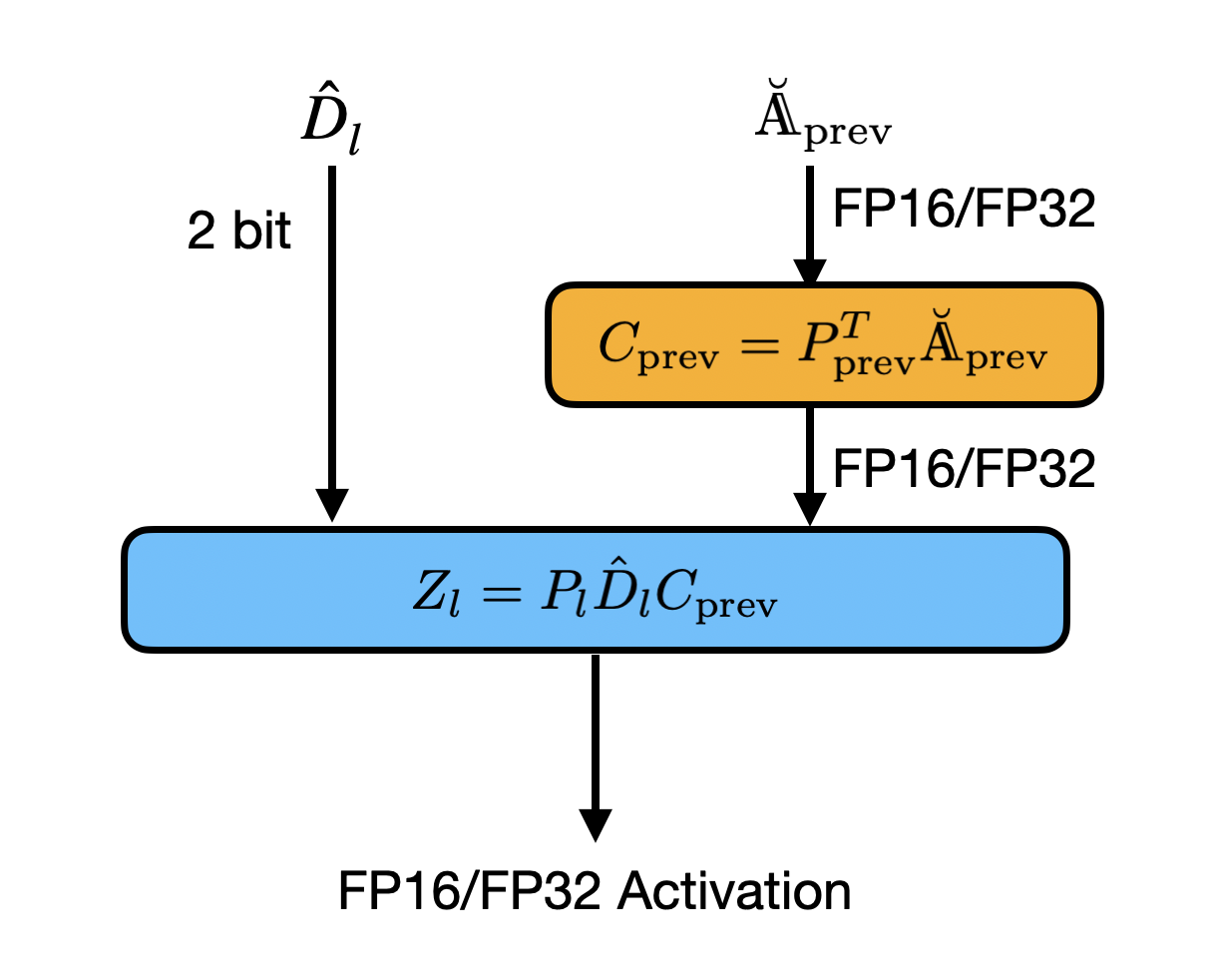
During inference, the quantized model is loaded into memory. At each layer, the inputs to the layer (${\breve{\mathds{A}}}_{prev}$) are first transformed into their Fusion Frame representations using the analysis operator ${\color[rgb]{0.1,0.0499999999999999,0.96}P^{T}_{\rm prev}}$. The FF representations are then transformed by the quantized weights ($D_{l}$) for this layer into the FF representations of the output. Finally the synthesis operator ${\color[rgb]{0.1,0.0499999999999999,0.96}P_{l}}$ is used to compute the layer outputs. Figure 3 shows this dequantization process and the bit widths of each of these operations for a single layer in a network.

Method	#bits	ViT				DeiT			Swin
		T	S	S/32	B	T	S	B	S	B	B/384
Full-Precision	32	75.46	81.39	75.99	85.10	72.16	79.85	81.98	82.88	84.67	86.02
PTQ4ViT	2	0.33	0.55	0.71	0.41	1.51	4.47	25.54	12.54	0.15	0.15
GPTQ	2	0.40	0.40	0.39	29.26	1.60	4.23	41.00	43.54	47.38	57.52
QuIP	2	1.42	21.98	19.00	77.54	12.93	51.62	75.51	71.58	74.91	79.85
QuIP (with our $2\sigma$ clip)	2	9.10	48.96	41.41	79.54	30.49	65.70	77.69	76.34	79.17	82.40
FrameQuant ($r=1.0$)	2	8.92	48.10	41.16	79.53	31.73	66.35	77.62	77.91	80.16	82.44
FrameQuant ($r=1.1$)	2.2	25.79	61.51	53.85	80.93	46.48	70.43	78.67	78.77	81.33	83.42
PTQ4ViT	3	18.32	36.18	22.20	21.43	51.73	69.65	75.35	73.01	69.46	70.68

Table 1: ImageNet-1k Top-1 validation accuracy of Tiny to Base sized Vision Transformer-based models when quantized to 2 (or 3) bits by different methods. FrameQuant with a redundancy factor of $r=1$ already performs better or on par with Quip Chee et al. (2023). With a slightly higher redundancy factor of $r=1.1$, we get the best performance of all the methods under consideration.

4 Experiments

We performed an extensive set of experiments comparing FrameQuant with several quantization baselines for Vision models and Language models. The goal is to assess (a) performance metrics of different methods on benchmark tasks and (b) how close low-bit quantization can approach the full precision performance with a small degree of representation redundancy. We use image classification task Deng et al. (2009) for Vision models and Perplexity for Language models.

We start with an introduction to our experimental setup. We present the evaluation results of FrameQuant on 15+ Vision Transformer architectures+configurations for image classification. Next, we conduct an ablation study on image classification task to better understand the behavior of different components of FrameQuant. We then present results on Language models such as OPT Zhang et al. (2022a) and Llama2 Touvron et al. (2023) by comparing perplexity and accuracy in downstream tasks. Please see the appendix for additional experiments.

4.1 Experimental Setup

Figure 3: Inference for a FrameQuant quantized model.

We evaluate our method on the ImageNet-1K classification task. For quantizing the model weights of the pre-trained models obtained from the Huggingface hub Wightman (2019), we use 128 images randomly selected images from the training dataset as calibration dataset $\mathcal{D}$. We quantize the parameter matrices of the layers sequentially from shallow layers to deep layers, similar to Frantar et al. (2023). After quantizing each layer, we pass the inputs to the layer again and send the output with the quantized weights to the next layer. Finally, we evaluate the quantized models on the ImageNet-1K validation dataset and report the top-1 accuracy. All our “base” experiments correspond to $2$ bits. We note that one of the baselines, PTQ4ViT Yuan et al. (2022), performs activation quantization together with weight quantization, but was not tested in the extreme $2$ bit quantization setting. To ensure fair comparisons to that method, we switch off activation quantization in their method and also add another experiment with $3$ bits.

4.2 Results on ImageNet Classification Task

Method	#bits	ViT		DeiT III		Swin
		L	H	L	H	L
Full-Precision	32	85.84	87.59	86.97	87.19	85.95
PTQ4ViT	2	37.05	00.18	2.14	55.57	-
GPTQ	2	63.08	42.63	68.43	28.20	71.69
QuIP	2	82.22	84.58	84.76	86.27	83.61
QuIP (our $2\sigma$ clip)	2	83.17	85.31	85.48	86.38	84.27
FrameQuant ($r=1.0$)	2	83.22	85.49	85.45	86.62	84.25
FrameQuant ($r=1.1$)	2.2	83.67	85.99	85.75	86.68	84.42
PTQ4ViT	3	81.26	78.92	83.63	85.39	-

Table 2: ImageNet-1K Top-1 validation accuracy of Large and Huge sized Vision Transformer-based models when quantized to 2 (or 3) bits by different methods.

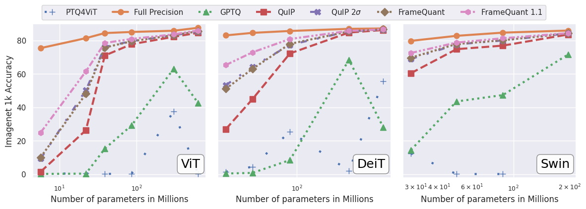
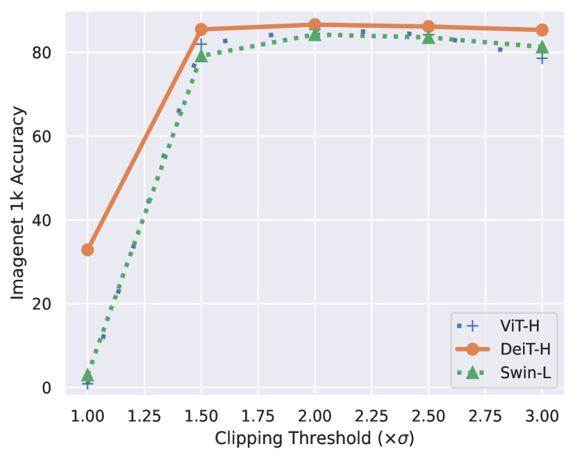
We use model architectures (including ViT Dosovitskiy et al. (2021), DeiT Touvron et al. (2021), DeiT III Touvron et al. (2022), and Swin Liu et al. (2021b)) and model sizes (including small, medium, large, huge) that are available on the Huggingface hub Wightman (2019). Our main highlight results are shown in Tables 1–2. Figure 4 shows the performance of the different classes of models on the ImageNet-1K dataset. We observed that clipping the weights at $2\sigma$ also helps QuIP Chee et al. (2023), so we include it as an additional baseline. Even with a redundancy factor of $r=1$, FrameQuant achieves better accuracy compared to most of the baselines under consideration. Further, with a redundancy factor of $r=1.1$, we outperform all baselines by a significant margin and are respectably close to the full precision model, underscoring the robustness of Fusion Frames in the presence of quantization noise. We observe that adding more redundancy to the Frame representations continues to improve the performance of the quantized models, especially when the models are small. See §A for more details. We note that the codebase for PTQ4ViT Yuan et al. (2022) was not compatible with the Swin-L model, so we could not report their performance for this model.

Figure 4: Validation accuracies of Vision Transformers on ImageNet-1K dataset. We can see FrameQuant closing the gap between the full precision model with increasing redundancy.

4.3 Ablation Study

Figure 5: The distribution of weights in a ViT layer and the $2\sigma$ thresholds for clipping.

In this section, we dissect FrameQuant to understand the contribution of different components of our algorithm. Table 3 shows the results of this experiment. We use GPTQ Frantar et al. (2023) as our starting point. With GPTQ Frantar et al. (2023) alone, the performance drops in the quantized models are significant: as high as $82\%$ for the DeiT III Touvron et al. (2022) Base model. Simply with the FF representation added (column TFF), we see improvements in performance across all models, with a maximum improvement of $56\%$ for DeiT III-H. We note that some of the smaller-sized models are yet to see all the benefits of FF representations. That is because these models have outliers in the weights (much larger than the remaining weights) which results in higher quantization errors. The FF representation yields a nice enough distribution that we can fit a Normal distribution. So, after we clip these weights at the $\pm 2\sigma$ level, we see improvements in performance because of the outlier removal. Finally, we add a redundancy factor of $r=1.1$ and the FF representations take advantage of this redundancy: we see the best performance across the board.

GPTQ	TFF	$2\sigma$ clip	Redundancy	ViT			DeiT III			Swin
			$r=1.1$	S	B	H	S	B	H	S	B	L
ON	OFF	OFF	OFF	$0.4$	$29.26$	$42.63$	$0.45$	$8.5$	$28.2$	$43.54$	$47.38$	$71.69$
ON	ON	OFF	OFF	$0.88$	$59.87$	$68.75$	$1.48$	$29.92$	$84.33$	$61.01$	$60.21$	$79.52$
ON	ON	ON	OFF	$48.10$	$79.53$	$85.49$	$51.13$	$77.99$	$86.62$	$77.91$	$80.16$	$84.25$
ON	ON	ON	ON	$\bm{61.51}$	$\bm{80.93}$	$\bm{85.99}$	$\bm{65.33}$	$\bm{80.91}$	$\bm{86.68}$	$\bm{78.77}$	$\bm{81.33}$	$\bm{84.42}$
			Full Precision	$81.39$	$85.1$	$87.59$	$83.06$	$85.7$	$87.19$	$82.79$	$84.7$	$85.95$

Table 3: Incremental impact of various steps in FrameQuant on ImageNet-1k accuracy for different Transformer models in Vision

Impact of Gaussian assumption on the weights distribution. Figure 5 shows a representative example of the distribution of weights in a model from the ViT family and why the $2\sigma$ clipping seems reasonable for capturing most of the mass. The weights distribution for models from DeiT and Swin Transformer are shown in Figure §14.

4.4 Results on Language Models

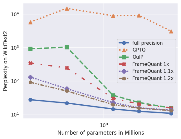
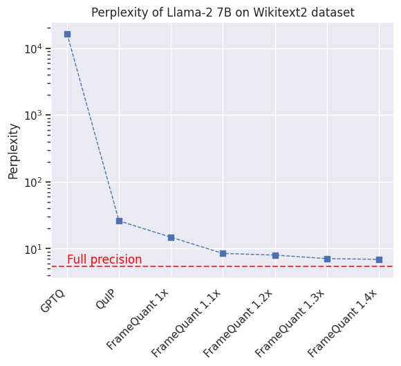
In this experiment, we evaluate the perplexity of quantized models from the OPT Zhang et al. (2022a) and Llama2 Touvron et al. (2023) family on two datasets - WikiText2 Merity et al. (2017) and C4 Raffel et al. (2020). Figure 6 shows the perplexity of models from the OPT family as the size is increased. We see that FrameQuant at $1\times$ redundancy performs better than all other quantization methods. With a redundancy factor of $1.1\times$, FrameQuant reduces the performance gap with the full precision models as suggested by the theory. We see similar results for models from the Llama2 family as well.

Method	bits	OPT				Llama2
		125M	1.3B	2.7B	6.7B	7B	70B
Full-Precision	16	27.65	14.62	12.47	10.86	5.68	3.32
GPTQ	2	5.7e3	8.9e3	9.1e3	3.1e3	6.4e3	140.5
QuIP	2	913.0	37.59	22.86	15.67	26.02	6.21
FrameQuant	2	345.7	30.54	20.67	15.72	14.85	5.50
FrameQuant	2.2	131.2	22.68	15.86	13.53	8.48	4.67

Table 4: Perplexity (lower is better) of Llama2 and OPT models on WikiText2 dataset when quantized to 2 (or 2.2) bits by different methods.

We also finetuned the Llama2-7B model quantized by various methods on diverse downstream tasks and observed a maximum accuracy boost of $41\%$ by FrameQuant at $r=1.1\times$ compared to vanilla GPTQ. Table 4 summarizes the perplexity of all the models under consideration on the WikiText2 Merity et al. (2017) dataset. Appendix §G provides all results on downstream tasks and additional datasets.

(a) Perplexity on WikiText2

(b) Perplexity on C4

Figure 6: Perplexity of models from OPT family on WikiText2 and C4 datasets. FrameQuant performs better than all other quantization methods under consideration. We can also see that the performance gap between the quantized models and the unquantized model goes down as the size of the models increases.

5 Discussion

We cover a few additional aspects that were not explicitly discussed thus far. (1) Can we reduce to one bit?This appears non-trivial. We performed experiments with redundancy of $1.8\times$ with $1$ bit per weight but were unsuccessful. For one bit, once the redundancy has exceeded $r=2$, it makes more sense to just use two bits. (2) Can FrameQuant run as QuIP?For each layer, if we choose a Fusion Frame with a redundancy factor $r=1$ and the random orthonormal basis $P_{l},P_{\rm prev}$, we get a setup similar to QuIP Chee et al. (2023) after removing the $2\sigma$ weight clipping. In this way, our method generalizes their approach. Hence, when QuIP is augmented with our $2\sigma$ clipping we see similar results to FrameQuant with $1\times$ redundancy. (3) Additional storage needed?: Since there are efficient deterministic algorithms to generate Fusion Frames, during inference, only knowledge of $(k,\rho,d)$ is needed. For rotation, we only need knowledge of the seed. Also, since many layers in a Transformer model have the same shape, these parameters can be shared across layers. Additional details on the storage benefits are given in §J.1 (4) Why is flexibility useful?If the performance hit at the two-bit level is unacceptable for an application, the only recourse currently is to move up to three bits for existing methods ($50\%$ increase). However, FrameQuant allows flexibility through the choice of the redundancy factor $r$. (5) Higher bitwidths?The main focus of this work is to evaluate 2-bit quantization of the weights in Vision and Language models and to check the benefits of applying Fusion Frames in terms of flexible bit-widths. Higher bit widths such as 3 or 4-bit quantization have been studied Frantar et al. (2023); Chee et al. (2023) and also used in practice Gerganov (2023). (6) Computational Complexity during Inference:The core FF-related compute is similar to alternatives Chee et al. (2023) with a small overhead related to the number of subspaces $k$. During inference, we need an additional compute of $\mathcal{O}(d^{2}(kr+\log{d}))$ for transforming the weights from the Fusion Frame representation space to the regular weight space. Any quantization scheme in the low-bit regime will incur a cost of $\mathcal{O}(d^{2})$ to transform the quantized weights by scaling and shifting them. More details are provided in §J.2.

6 Conclusions

The paper describes FrameQuant, a Frames based algorithm for flexible low-bit quantization. Quantization is motivated by the need to efficiently serve Large Language Models on heterogeneous devices and flexibility here means that while we retain the option to go as low as two bits; depending on the needs of the downstream task, the user also has the flexibility to seek models with a net footprint of 2.x bits on average. Across most widely used Vision Transformer models and Large Language models, we find that effective quantization is possible with only a small loss in performance relative to the full-precision model. Further, flexibility for a minor increase in redundancy is available and uniformly helps close the gap with full precision models. We observe, consistent with the literature, that quantization to low bit width is more favorable for larger models (in terms of a performance hit) than a similar quantization applied to smaller models. While some benefits (e.g., model loading time, loading larger models) are immediate, tighter integration with the hardware can unlock far more efficiency gains. The code is publicly available.

Figure 7: Effect of flexibility/redundancy on activation maps for ViT-S. Figure showing attention maps of ViT-S as the redundancy is increased from $r=1$ to $r=1.3$ in the increments of $0.1$ from left to right. The first column shows the image and the ground truth label, and the rest of the columns show the regions that the model is attending to in the final transformer block. We see that as the redundancy is increased, the model gets more focused, with the attention regions concentrating on the objects of interest.

In this Appendix, we provide additional details related to the experiments reported in the main paper. This Appendix is organized as follows. In Section A we analyze the impact of redundancy on the performance of the model in terms of classification accuracy on the ImageNet-1k dataset. In Section B, we study this effect on the performance of Vision Transformer models, evaluated using activation maps. Next, in Section C, we study the effect of the size of the calibration data used for quantizing various Vision Models. In Section D, we analyze the choice of the $2\sigma$ threshold for clipping the weights during quantization. We provide empirical evidence for different classes of Vision models. Section E shows the distribution of weights in the DeiT and Swin Transformer models. In Section F, we present a framework for quantizing activations and show how the FF representation of activations inherently addresses the key pain points described in previous works. In Section G, we present more experiments on Language models on different datasets and downstream tasks as mentioned in the main paper. Then, in Section H, we provide an expanded synopsis of the theoretical results that apply to our setting, as briefly described in the main paper. In Section I we provide a brief synopsis of the algorithm used to generate a TFF for the curious reader. Finally in section J we give a detailed analysis of the storage benefits of FrameQuant and the computational complexity during inference.

Appendix A Impact of redundancy in representations

We consider the impact of redundancy in our Frame representation moving forward from 2 bits, incrementally increasing redundancy. Table 5 shows the performance of different models at different levels of redundancy. We observe that for large models, the original performance without any redundancy was already high, and adding redundancy did not impact their performance significantly. However, this is not the case for smaller models. Here, we see significant performance improvements (around $+21\%$ for the ViT-S model).

Redundancy	bits	ViT			DeiT III			Swin
		S	B	H	S	B	H	S	B	L
$r=1.00$	$(2.0~{}\text{bits})$	$48.10$	$79.53$	$85.49$	$51.13$	$77.99$	$86.62$	$77.91$	$80.16$	$84.25$
$r=1.05$	$(2.1~{}\text{bits})$	$56.19$	$79.97$	$85.67$	$58.74$	$79.59$	$86.58$	$78.47$	$80.41$	$84.26$
$r=1.10$	$(2.2~{}\text{bits})$	$61.51$	$80.93$	$85.99$	$65.33$	$80.91$	$86.68$	$78.77$	$81.33$	$84.42$
$r=1.15$	$(2.3~{}\text{bits})$	$65.17$	$81.27$	$86.04$	$69.54$	$81.69$	$86.67$	$78.87$	$81.88$	$84.51$
$r=1.20$	$(2.4~{}\text{bits})$	$66.53$	$81.59$	$86.11$	$71.07$	$81.98$	$86.61$	$79.56$	$82.02$	$84.56$
$r=1.25$	$(2.5~{}\text{bits})$	$68.57$	$81.74$	$86.06$	$73.48$	$82.51$	$86.55$	$79.99$	$82.26$	$84.51$
$r=1.30$	$(2.6~{}\text{bits})$	$69.02$	$81.77$	$85.99$	$74.40$	$82.54$	$86.38$	$79.92$	$82.39$	$84.65$
Full Precision	-	$81.39$	$85.1$	$87.59$	$83.06$	$85.7$	$87.19$	$82.79$	$84.7$	$85.95$

Table 5: Performance of various quantized models on ImageNet-1K classification task as the redundancy in FrameQuant is increased. We see that increasing the redundancy closes the gap between the performance of the quantized model and the Full precision model

Appendix B Does redundancy impact attention maps?

Figure 8: Trend of accuracies in small size models as we increase the redundancy

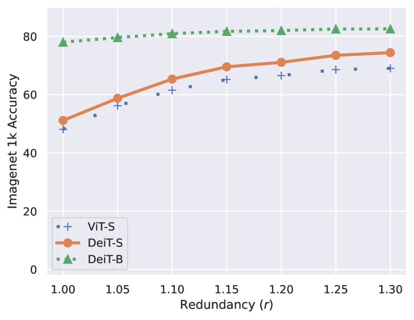
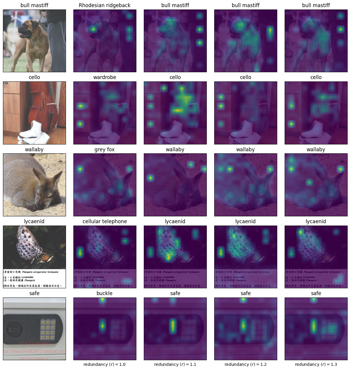
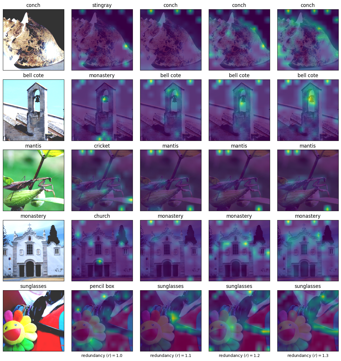
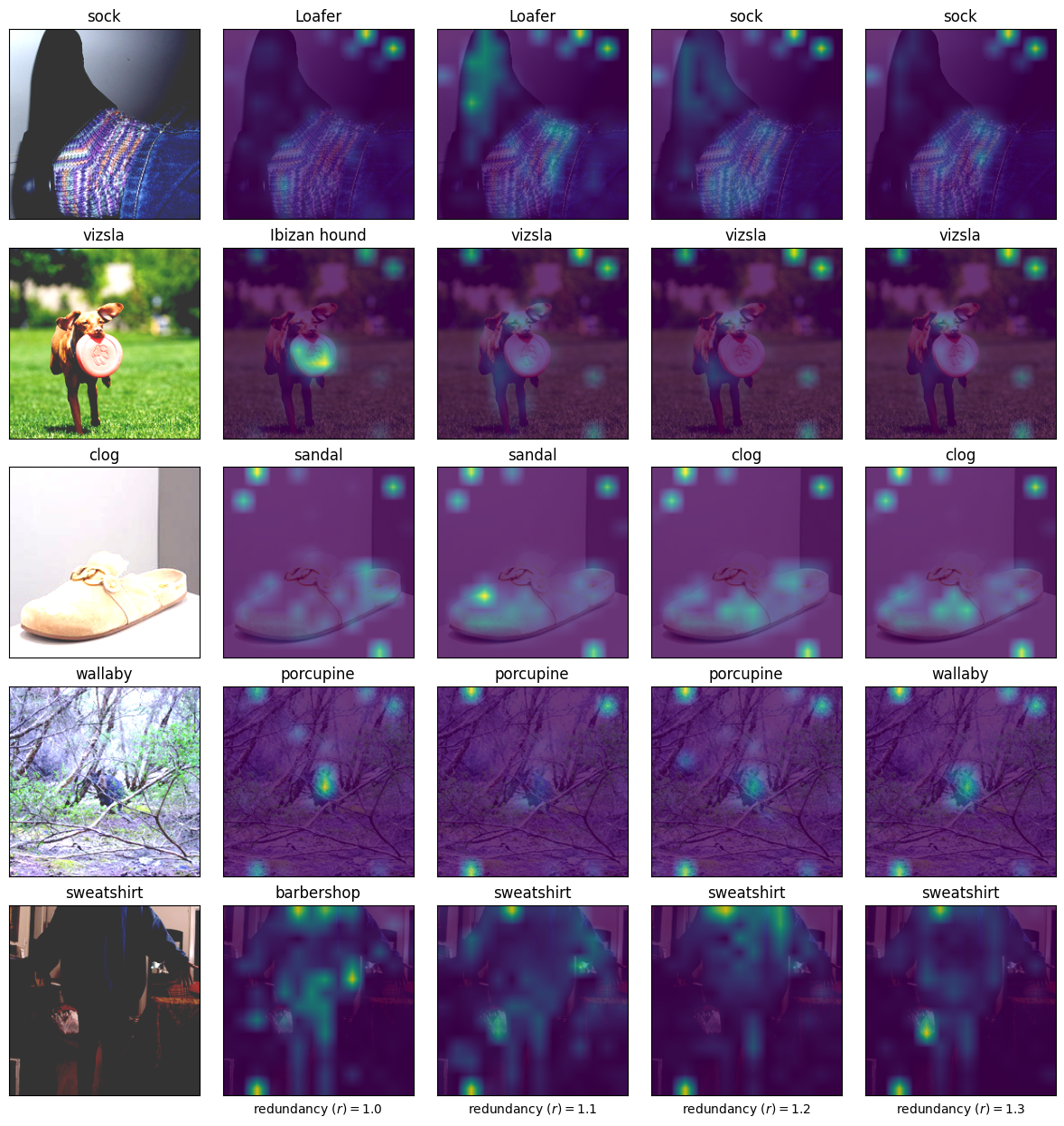
In the main paper, we discussed how the performance of the models improves as we increase the redundancy in the Fusion Frames during quantization. This section provides additional details on how redundancy affects the attention maps of Vision Transformers from different classes. We will focus mainly on the small and base models where we see significant improvement in the validation accuracy on ImageNet as we increase the redundancy. Figures 7, 9 and 10 show the attention maps of Vit-S, DeiT III -S, and Deit III - B models respectively. These models show an improvement in the range of $4.55\%$ to $23.27\%$ as we increase the redundancy from $r=1$ to $r=1.3$. This is reflected in the attention maps as well. We see that as the redundancy increases, the attention regions systematically concentrate on the objects of interest. This is consistent with the improvement in accuracy and can also be seen in Figure 8.

Figure 9: Effect of flexibility/redundancy on activation maps for DeiT III-S. Figure showing attention maps of DeiT III -S as the redundancy is increased from $r=1$ to $r=1.3$ in the increments of $0.1$ from left to right.

Figure 10: Effect of flexibility/redundancy on activation maps for DeiT III-B. Figure showing attention maps of DeiT III -B as the redundancy is increased from $r=1$ to $r=1.3$ in the increments of $0.1$ from left to right.

Appendix C Does the calibration set size matter?

We noted that a small calibration set size was sufficient in the main paper. In this section, we report on experiments varying the number of calibration images and observe the performance of different classes of models on ImageNet-1K. We use a redundancy factor of $r=1$ in this experiment. Table 6 shows the validation accuracies for different classes of models as the number of calibration images is increased from $128$ to $256$. We can see that performance improvement is only seen in small models from the ViT and DeiT III classes. So, we will focus on reporting results for these models. Figure 11 shows the accuracies of ViT-S and DeiT III-S models as the number of calibration images is increased from $128$ to $512$. We can see that there is a small improvement as the number of images is increased from $128$ to $200$, but the benefits taper off quickly as we increase it further. This shows that if access to the calibration is not limited, a small increase in the number of images used for quantization can provide benefits in terms of the final accuracies of the models, especially for smaller models.

Appendix D How does $2\sigma$  Clipping affect performance?

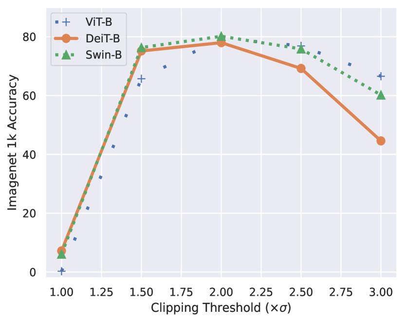
In the main paper, we discussed a simple clipping threshold at the $2\sigma$ level. In this section, we analyze the benefits of this choice and its effect on the performance of different classes of models on ImageNet-1K. As in the previous section, we use a redundancy factor of $r=1$ for these experiments and focus on the impact of clipping the weights at different levels based on their distribution. Figure 12 shows the accuracies of different classes of models as the threshold for the weights is varied from $\pm\sigma$ to $\pm 3\sigma$. We can see that the performance of all the models peaks in the neighborhood of $\pm 2\sigma$. Clipping at $\pm\sigma$ restricts the range of the weights too aggressively, incurring errors. At $\pm 3\sigma$ level, which is close to allowing the entire range, we are stretching the effective scale of the weights to allow all the extreme entries to be represented within the range. This in turn increases the width of the quantization levels, which affects the majority of the weights impacting performance. $\pm 2\sigma$ seems to be the sweet spot.

#images	ViT			DeiT III			Swin
	S	B	H	S	B	H	S	B	L
$128$	$48.1$	$79.5$	$85.4$	$51.1$	$77.9$	$86.6$	$77.9$	$80.1$	$84.2$
$200$	$51.4$	$79.8$	$85.6$	$53.7$	$78.3$	$86.6$	$77.6$	$80.1$	$84.0$
$256$	$51.6$	$79.8$	$85.7$	$54.7$	$79.0$	$86.4$	$77.9$	$80.6$	$84.3$

Table 6: ImageNet-1K Top-1 validation accuracies of models from different classes as the number of calibration images is increased.

Figure 11: Trend of accuracies in small size models as we increase the number of calibration images

(a) Accuracies of Small models

(b) Accuracies of Base models

(c) Accuracies of Large models

Figure 12: Figure showing the impact of clipping at different thresholds based on $\sigma$

(a) Activations after the first block in ViT-M

(b) FF representations of ViT-M first block activations

Figure 13: Activations of the first Transformer Block of Vit-M model and their FF representations. We can see the outliers in the activations (shown in red) on the left, while the FF representations are well-behaved.

Appendix E Distribution of weights in the DeiT and Swin Transformer models

This section presents the distribution of the weights in the DeiT and Swin Transformer models. Figure 14 shows the distribution of weights in a linear layer from the DeiT and Swin Transformer families. We can see that the distribution is well behaved and the $2\sigma$ threshold captures most of the mass well.

(a) Weight distribution in DeiT

(b) Weight distribution in Swin Transformer

Figure 14: Weights distribution in DeiT and Swin Transformer models.

Appendix F FrameQuant for Activation Quantization?

In the main paper, we restricted the experimental setup to weight quantization for meaningful comparisons to recent PTQ papers. This is because activation quantization in this low-bit regime has not been reported and each baseline will need modifications to report the best possible results. In this section, we provide some details regarding applying FrameQuant for activation Quantization with the caveat that a comprehensive head-to-head comparison to all reported baselines is difficult for the reasons above.

Since we operate in the FF representation space, we first compute the FF representations of the previous layer activations,

$${\color[rgb]{0,1,0}C_{\rm prev}}={\color[rgb]{0,1,0}P_{\rm prev}^{T}A_{\rm prev}}$$ (10)

and quantize these directly. Also, since activation quantization happens dynamically, during inference time, we keep the activation quantization procedure simple and just use the nearest rounding method. This can be written as:

$${\color[rgb]{0,1,0}\bar{C}_{\rm prev}}=\lfloor\frac{{\color[rgb]{0,1,0}C_{\rm prev}}}{\Delta_{C}}\rceil,\quad\Delta_{C}=\frac{\max{|{\color[rgb]{0,1,0}C_{\rm prev}}|}}{2^{\rm N-1}-1}$$ (11)

where ${\color[rgb]{0,1,0}\bar{C}_{\rm prev}}$ is in INT8 form and is the quantized version of the FF representations of the activations (${\color[rgb]{0,1,0}C_{\rm prev}}$). $\lfloor\cdot\rceil$ represents nearest rounding. We can substitute with $\lfloor\cdot\rfloor$ or $\lceil\cdot\rceil$ to get the floor or the ceil operation. We have found that FrameQuant-based quantization of ${\color[rgb]{0,1,0}\bar{C}_{\rm prev}}$ to eight, six or even four bits works well.

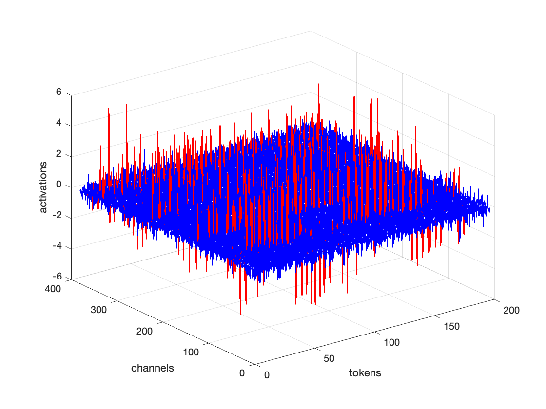
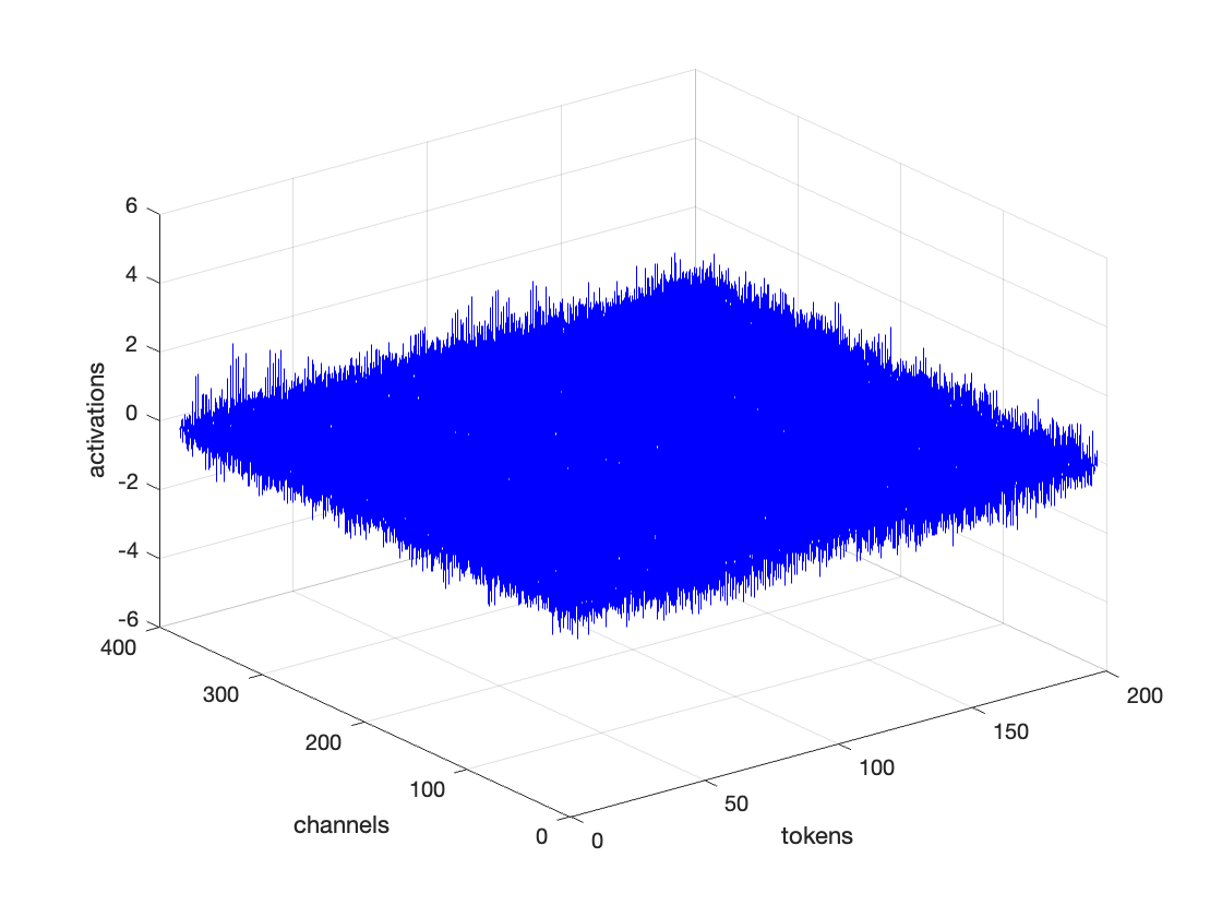
Benefits of well-behaved FF representations. As noted by Xiao et al. [2023], we also observe that the activations have large outliers in some of the channels whose values are more than $100\times$ larger than the activations of other channels on average and this behavior is consistent across the tokens. This is shown in Figure 13(a) So, to quantize the outliers, we need a large-scale factor $\Delta_{C}$ which will quantize all small values to zero. The other option is to use per-channel quantization – where we have different scale factors for different channels. This would solve the outlier problem, but it is not ideal because we cannot use integer kernels for matrix multiplications in the Linear Layers. To use integer arithmetic for the matrix multiplications in the Linear layers, we can only perform per-token quantization for the activations and per-channel quantization for the weights. To solve this problem, Xiao et al. [2023] shifts the scale from activations to weights that are well-behaved. They dynamically search for different amounts of shifts between the weights and activations using a calibration set and use that during inference. Since we operate in the FF representation space, we observe that after we compute the FF representations of the activations, they are well-behaved. Figure 13(b) shows the FF representation of activation of the first Transformer block in the ViT-M model. So, we do not need to perform further scaling to reduce the range. This makes FrameQuant to be amenable to activation quantization if necessary in practice.

Appendix G Additional Experiments on Language models

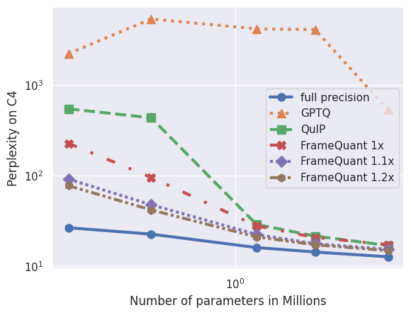
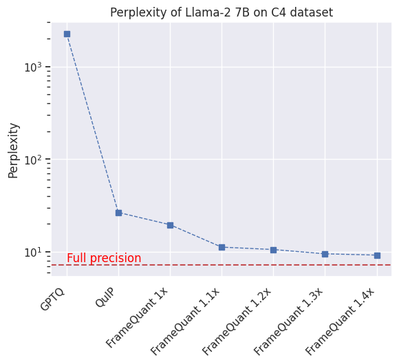
G.1 Evaluation on the C4 dataset

This section is a continuation of section 4.4. Here, we present the perplexity of different models from OPT and Llama2 classes on the C4 Raffel et al. [2020] dataset. Consistent with our previous experiments, we see that FrameQuant with $1\times$ the redundancy performs better than all the methods under consideration. With an additional redundancy of $r=1.1\times$, FrameQuant closes the gap between the full precision model across all the sizes from different families of Large Language Models. The results are shown in table 7.

Method	#bits	OPT					Llama2
		125M	350M	1.3B	2.7B	6.7B	7B	70B
Full-Precision	16	$26.56$	$22.58$	$16.07$	$14.34$	$12.71$	$7.26$	$5.71$
GPTQ	2	$2203.89$	$5325.65$	$4139.91$	$4058.41$	$528.41$	$2265.09$	$68.83$
QuIP	2	$543.63$	$432.56$	$28.91$	$21.49$	$16.92$	$26.61$	$8.65$
FrameQuant ($r=1.0$)	2	$226.15$	$95.38$	$27.90$	$20.74$	$17.28$	$19.62$	$7.85$
FrameQuant ($r=1.1$)	2.2	$\bm{91.29}$	$\bm{47.62}$	$\bm{22.39}$	$\bm{17.75}$	$\bm{15.33}$	$\bm{11.23}$	$\bm{6.86}$

Table 7: Perplexity (smaller the better) of Llama2 and OPT models on C4 dataset when quantized to 2 (or 2.2) bits by different methods.

G.2 Perplexity of Quantized Llama2 7B

Figure 15 shows the perplexity of Llama2-7B model quantized by different quantization schemes. We see that FrameQuant with a redundancy of 1x already performs better than all other methods. With increasing redundancy, the performance becomes closer to the Full precision model.

(a) Perplexity of Llama2-7B model on WikiText2

(b) Perplexity of Llama2-7B model on C4 dataset

Figure 15: Perplexity of Llama2-7B model on WikiText2 and C4 datasets. FrameQuant performs better than all quantization methods tested. With increasing redundancy, we see that the performance of the model also improves as indicated by the theory.

G.3 Performance on Downstream tasks

In this experiment, we finetune the Llama2-7B model on downstream tasks. We ran experiments on ARC challenge, ARC easy Clark et al. [2018], BoolQ Clark et al. [2019], HellaSwag Zellers et al. [2019], PIQA Bisk et al. [2020] and WinoGrande Sakaguchi et al. [2021]. We used LM-evaluation harness Gao et al. [2023] for running our experiments on these diverse tasks. The results are presented in table 8. We can see that again in line with our previous experiments, the LLM quantized with FrameQuant with no redundancy already performs better than all the other methods on the downstream tasks. With added redundancy, this performance goes up across all the tasks under consideration. Based on our previous experiments and as observed in Chee et al. [2023], we expect the performance gap between the full precision model and the quantized model to go down as the size of the models increases.

Method	#bits	ARC (challenge)	ARC (easy)	BoolQ	HellaSwag	PIQA	WinoGrande
Full-Precision	16	$43.43$	$76.35$	$77.71$	$57.16$	$78.07$	$69.06$
GPTQ	2	$22.44$	$24.58$	$41.19$	$25.93$	$51.85$	$50.43$
QuIP	2	$22.27$	$42.76$	$50.31$	$34.04$	$61.75$	$52.64$
FrameQuant ($r=1.0$)	2	$23.98$	$55.39$	$63.52$	$36.76$	$66.65$	$55.80$
FrameQuant ($r=1.1$)	2.2	31.91	65.53	67.95	46.46	73.07	63.61

Table 8: Evaluating Llama2-7B model quantized with different methods on a range of downstream tasks.

Appendix H Robustness guarantees

We provide additional details on two specific results (mentioned in the main paper) that apply to our construction. We encourage the interested reader to refer to Christensen [2018], Casazza and Kutyniok [2012] for a more comprehensive treatment of the topic.
LMMSE estimation from fusion frame measurements. For a given layer $l$ FrameQuant quantizes the transformed weights matrix $D_{l}$ which is given by $D_{l}={\color[rgb]{0.1,0.0499999999999999,0.96}P_{l}^{T}}(\Theta_{l}{\color[rgb]{0.1,0.0499999999999999,0.96}P_{\rm prev}})$. We can treat $\hat{D}_{l}$ as a projection of $\Theta_{l}{\color[rgb]{0.1,0.0499999999999999,0.96}P_{\rm prev}}$ which is corrupted by noise. During inference, the activations of this layer are given by $Z_{l}={\color[rgb]{0.1,0.0499999999999999,0.96}P_{l}}\hat{D}_{l}{\color[rgb]{0,1,0}C_{\rm prev}}$. But, can we do better? Instead of directly applying the synthesis operator ${\color[rgb]{0.1,0.0499999999999999,0.96}P_{l}}$ to compute $Z_{l}$ from its FF representations $\hat{D}_{l}{\color[rgb]{0,1,0}C_{\rm prev}}$, we can design a simple linear filter $F$ that minimizes the MSE in $Z_{l}$ because we are using a quantized $\hat{D}_{l}$. The final expression for the computation of the output of the layer will be $Z_{l}=F\hat{D}_{l}{\color[rgb]{0,1,0}C_{\rm prev}}$. This linear MSE minimizer $F$ is known to be the Wiener Filter and has a closed-form expression with various levels of approximation. The following theorem states that the Wiener filter minimizes MSE when the Fusion Frame is tight.

Theorem H.1.

Kutyniok et al. [2009] For the model described above, the MSE in linearly estimating the signal from its noisy projections is minimized when the Fusion Frame is tight

Consistent Reconstruction. Assuming the same mode of representing the modified weights $D_{l}$ as above, during inference, we can get a consistent estimate of the weights ($\hat{\Theta}_{l}$) from $\hat{D}_{l}$ if one were to solve a linear program for $\hat{X}$

$$\begin{bmatrix}{\color[rgb]{0.1,0.0499999999999999,0.96}P_{l}}\\ {\color[rgb]{0.1,0.0499999999999999,0.96}-P_{l}}\end{bmatrix}\hat{X}_{l}\leq\begin{bmatrix}\frac{\Delta}{2}+\hat{D}_{l}\\ \frac{\Delta}{2}-\hat{D}_{l}\end{bmatrix},$$

where $\Delta$ is the quantization level. Here, the constraints in the Linear Program make sure that $\hat{X}$ belongs to the regions where valid unquantized values must lie, thereby removing the out-of-sub-space error Goyal et al. [1998]. We can get the estimated weights from $\hat{X}_{l}$ as $\hat{\Theta}_{l}=\hat{X}_{l}{\color[rgb]{0.1,0.0499999999999999,0.96}P^{T}_{\rm prev}}$. Using this consistent reconstruction yields estimates with an MSE which is upper bounded by $\mathcal{O}(1/r^{2})$ Goyal et al. [1998]

Appendix I Synopsis of Construction of Tight Fusion Frames

Here, we give a brief synopsis of an algorithm for generating Tight Fusion Frames for the curious reader. Casazza et al. [2011] was the first to introduce a systematic method for constructing UNTFs (Unit Norm Tight Frames) that play a key role in constructing Tight Fusion Frames. They also characterize the $(k,\rho,d)$ values for which a Tight Fusion Frame exists. Whenever such a TFF exists, we can construct Tight Fusion Frames by using their algorithm. There are two main parts to the algorithm.

1. Play Spectral Tetris to generate a UNTF of $d$ elements in $\mathbb{C}^{\rho}$

2. Modulate this UNTF with complex roots of unity to generate a $(k,\rho,d)$ TFF for $\mathbb{C}^{d}$

So, the first step is to generate a “smaller” frame and in the next step, we modulate the smaller frame to generate a “larger” Tight Fusion Frame. After generating a TFF for $\mathbb{C}^{d}$ we can easily extend it to the Real Field by applying the entrywise map $x+iy\mapsto\begin{bmatrix}x&-y\\ y&x\end{bmatrix}$. We describe the algorithm with the help of an example for the simplicity of explanation. We aim to construct a (5,4,11) TFF. So, $k=5,\rho=3,d=11$.

I.1 Spectral Tetris

As the name suggests UNTFs are Tight frames where each frame vector has a unit norm. We construct a $4\times 11$ matrix $F$ whose columns are the frame vectors for $\mathbb{C}^{4}$ which satisfies

• Columns of unit norm

• Orthogonal rows, meaning $FF^{*}$ is diagonal

• Rows of constant norm, meaning $FF^{*}$ is a constant multiple of identity matrix with the constant being $\frac{11}{4}$

We start with a matrix

$$F=\setcounter{MaxMatrixCols}{11}\begin{bmatrix}1&1&?&?&?&?&?&?&?&?&?\\ ?&?&?&?&?&?&?&?&?&?&?\\ ?&?&?&?&?&?&?&?&?&?&?\\ ?&?&?&?&?&?&?&?&?&?&?\\ \end{bmatrix}$$

This leaves a norm of $\frac{11}{4}-2=\frac{3}{4}$ to be filled in the first row. This can easily be added using a $2\times 2$ matrix $T(x)$ where $x=\frac{3}{4}$. $T(x)$ is defined as:

$$T(x)\vcentcolon=\frac{1}{\sqrt{2}}\begin{bmatrix}\sqrt{x}&\sqrt{x}\\ \sqrt{2-x}&-\sqrt{2-x}\end{bmatrix},\quad\quad T(x)T^{*}(x)=\begin{bmatrix}x&0\\ 0&2-x\end{bmatrix}$$

After inserting $T(x)$, $F$ is now

$$F=\setcounter{MaxMatrixCols}{11}\begin{bmatrix}1&1&\frac{\sqrt{3}}{\sqrt{8}}&\frac{\sqrt{3}}{\sqrt{8}}&0&0&0&0&0&0&0\\ 0&0&\frac{\sqrt{5}}{\sqrt{8}}&-\frac{\sqrt{5}}{\sqrt{8}}&?&?&?&?&?&?&?\\ 0&0&0&0&?&?&?&?&?&?&?\\ 0&0&0&0&?&?&?&?&?&?&?\\ \end{bmatrix}$$

Then we continue adding ones in row two until the norm becomes less than $\frac{11}{4}$.

$$F=\setcounter{MaxMatrixCols}{11}\begin{bmatrix}1&1&\frac{\sqrt{3}}{\sqrt{8}}&\frac{\sqrt{3}}{\sqrt{8}}&0&0&0&0&0&0&0\\ 0&0&\frac{\sqrt{5}}{\sqrt{8}}&-\frac{\sqrt{5}}{\sqrt{8}}&1&?&?&?&?&?&?\\ 0&0&0&0&0&?&?&?&?&?&?\\ 0&0&0&0&0&?&?&?&?&?&?\\ \end{bmatrix}$$

Now we insert $T(x)$ with the remaining norm. We repeat this process until all the rows are filled. The Final $F$ is given by

$$F=\setcounter{MaxMatrixCols}{11}\begin{bmatrix}1&1&\frac{\sqrt{3}}{\sqrt{8}}&\frac{\sqrt{3}}{\sqrt{8}}&0&0&0&0&0&0&0\\ 0&0&\frac{\sqrt{5}}{\sqrt{8}}&-\frac{\sqrt{5}}{\sqrt{8}}&1&\frac{\sqrt{2}}{\sqrt{8}}&\frac{\sqrt{2}}{\sqrt{8}}&0&0&0&0\\ 0&0&0&0&0&\frac{\sqrt{6}}{\sqrt{8}}&-\frac{\sqrt{6}}{\sqrt{8}}&1&\frac{\sqrt{7}}{\sqrt{8}}&\frac{\sqrt{7}}{\sqrt{8}}&0\\ 0&0&0&0&0&0&0&0&\frac{\sqrt{7}}{\sqrt{8}}&-\frac{\sqrt{7}}{\sqrt{8}}&1\\ \end{bmatrix}$$

I.2 Modulation

In the second step, we modulate the $F$ matrix with complex roots of unity, one subspace at a time. So, for each $k_{i}=0,1,2,\dots k-1$, we construct a row vector

$$w_{k_{i}}=[\left(e^{\frac{i2\pi k_{i}}{k}}\right)^{0}\left(e^{\frac{i2\pi k_{i}}{k}}\right)^{1}\left(e^{\frac{i2\pi k_{i}}{k}}\right)^{2}\dots\left(e^{\frac{i2\pi k_{i}}{k}}\right)^{d-1}]$$

We multiply each row of $F$ with $w_{k_{i}}$ to generate the orthogonal basis for different subspaces indexed by $k_{i}$. Theorem $14$ by Casazza et al. [2011] proves that the Fusion Frames generated by this algorithm are Tight. The Final Fusion Frame vectors are shown in Table 9.

$$\setcounter{MaxMatrixCols}{11}\begin{bmatrix}[l]1&1&\frac{\sqrt{3}}{\sqrt{8}}&\frac{\sqrt{3}}{\sqrt{8}}&0&0&0&0&0&0&0\\ 1&\omega&\frac{\sqrt{3}}{\sqrt{8}}\omega^{2}&\frac{\sqrt{3}}{\sqrt{8}}\omega^{3}&0&0&0&0&0&0&0\\ 1&\omega^{2}&\frac{\sqrt{3}}{\sqrt{8}}\omega^{4}&\frac{\sqrt{3}}{\sqrt{8}}\omega&0&0&0&0&0&0&0\\ 1&\omega^{3}&\frac{\sqrt{3}}{\sqrt{8}}\omega&\frac{\sqrt{3}}{\sqrt{8}}\omega^{4}&0&0&0&0&0&0&0\\ 1&\omega^{4}&\frac{\sqrt{3}}{\sqrt{8}}\omega^{3}&\frac{\sqrt{3}}{\sqrt{8}}\omega^{2}&0&0&0&0&0&0&0\\ 0&0&\frac{\sqrt{5}}{\sqrt{8}}&-\frac{\sqrt{3}}{\sqrt{8}}&1&\frac{\sqrt{2}}{\sqrt{8}}&\frac{\sqrt{2}}{\sqrt{8}}&0&0&0&0\\ 0&0&\frac{\sqrt{5}}{\sqrt{8}}\omega^{2}&-\frac{\sqrt{3}}{\sqrt{8}}\omega^{3}&\omega^{4}&\frac{\sqrt{2}}{\sqrt{8}}&\frac{\sqrt{2}}{\sqrt{8}}\omega&0&0&0&0\\ 0&0&\frac{\sqrt{5}}{\sqrt{8}}\omega^{4}&-\frac{\sqrt{3}}{\sqrt{8}}\omega&\omega^{3}&\frac{\sqrt{2}}{\sqrt{8}}&\frac{\sqrt{2}}{\sqrt{8}}\omega^{2}&0&0&0&0\\ 0&0&\frac{\sqrt{5}}{\sqrt{8}}\omega&-\frac{\sqrt{3}}{\sqrt{8}}\omega^{4}&\omega^{2}&\frac{\sqrt{2}}{\sqrt{8}}&\frac{\sqrt{2}}{\sqrt{8}}\omega^{3}&0&0&0&0\\ 0&0&\frac{\sqrt{5}}{\sqrt{8}}\omega^{3}&-\frac{\sqrt{3}}{\sqrt{8}}\omega^{2}&\omega&\frac{\sqrt{2}}{\sqrt{8}}&\frac{\sqrt{2}}{\sqrt{8}}\omega^{4}&0&0&0&0\\ 0&0&0&0&0&\frac{\sqrt{6}}{\sqrt{8}}&-\frac{\sqrt{6}}{\sqrt{8}}&1&\frac{\sqrt{7}}{\sqrt{8}}&\frac{\sqrt{7}}{\sqrt{8}}&0\\ 0&0&0&0&0&\frac{\sqrt{6}}{\sqrt{8}}&-\frac{\sqrt{6}}{\sqrt{8}}\omega&\omega^{2}&\frac{\sqrt{7}}{\sqrt{8}}\omega^{3}&\frac{\sqrt{7}}{\sqrt{8}}\omega^{4}&0\\ 0&0&0&0&0&\frac{\sqrt{6}}{\sqrt{8}}&-\frac{\sqrt{6}}{\sqrt{8}}\omega^{2}&\omega^{4}&\frac{\sqrt{7}}{\sqrt{8}}\omega&\frac{\sqrt{7}}{\sqrt{8}}\omega^{3}&0\\ 0&0&0&0&0&\frac{\sqrt{6}}{\sqrt{8}}&-\frac{\sqrt{6}}{\sqrt{8}}\omega^{3}&\omega&\frac{\sqrt{7}}{\sqrt{8}}\omega^{4}&\frac{\sqrt{7}}{\sqrt{8}}\omega^{2}&0\\ 0&0&0&0&0&\frac{\sqrt{6}}{\sqrt{8}}&-\frac{\sqrt{6}}{\sqrt{8}}\omega^{4}&\omega^{3}&\frac{\sqrt{7}}{\sqrt{8}}\omega^{2}&\frac{\sqrt{7}}{\sqrt{8}}\omega^{1}&0\\ 0&0&0&0&0&0&0&0&\frac{\sqrt{7}}{\sqrt{8}}&-\frac{\sqrt{7}}{\sqrt{8}}&1\\ 0&0&0&0&0&0&0&0&\frac{\sqrt{7}}{\sqrt{8}}\omega^{3}&-\frac{\sqrt{7}}{\sqrt{8}}\omega^{4}&1\\ 0&0&0&0&0&0&0&0&\frac{\sqrt{7}}{\sqrt{8}}\omega&-\frac{\sqrt{7}}{\sqrt{8}}\omega^{3}&1\\ 0&0&0&0&0&0&0&0&\frac{\sqrt{7}}{\sqrt{8}}\omega^{4}&-\frac{\sqrt{7}}{\sqrt{8}}\omega^{2}&1\\ 0&0&0&0&0&0&0&0&\frac{\sqrt{7}}{\sqrt{8}}\omega^{2}&-\frac{\sqrt{7}}{\sqrt{8}}\omega&1\\ \end{bmatrix}$$

Table 9: $\bm{(5,4,11)}$-TFF for $\mathbb{C}^{11}$. Here, $\omega=e^{i2\pi/5}$. Each pair of rows belongs to the same subspace if their indices differ by a multiple of 5

Appendix J Storage benefits and Computational complexity during inference

J.1 Storage benefits

Consider an example where we are quantizing a weight matrix $\Theta_{l}$ of dimension $1024\times 1024$ using FrameQuant with a redundancy factor of $r=1.1\times$. The size of the original matrix using FP32 is 4MB. After transforming the weights to map within the FF representation space, the transformed weights $D_{l}$ have dimensions $1126\times 1126$, which are quantized and represented using 2 bits. This quantized weight $\hat{D}_{l}$ has a size of 0.3MB. Along with the quantized weights, we need to store the bias and scale values for each row leading to an additional storage of 1024 FP32 values, which will incur an additional cost of 0.007MB. All this sums up to a storage of 0.307MB from an initial 4MB giving a savings of 13x in the storage requirements. Since we can generate the Fusion Frames on the fly, we just need to store the $(k,\rho,d)$ values, and a seed to generate the random rotation matrix which incurs negligible storage costs.

J.2 Computational Complexity during Inference

Consider a linear layer in a transformer model with weights $\Theta_{l}$ of dimensions $d\times d$. Using FrameQuant these weights are transformed to $D_{l}$ and the quantized weights $\hat{D}_{l}$ are stored. Let the parameters of the TFF used for quantization be $(k,\rho,d)$. As a recap, $k$ is the number of subspaces, $\rho$ is the dimension of each subspace and $d$ is the dimension of the Hilbert space we are operating in. So, the redundancy in Frame representations is $r=\frac{k\rho}{d}$. Let, ${\color[rgb]{0.1,0.0499999999999999,0.96}T_{l}},{\color[rgb]{0.1,0.0499999999999999,0.96}T_{\rm prev}}\in\mathbb{R}^{d\times k\rho}$ be the vectorized Orthonormal basis for the current layer, and the previous layer respectively. During inference, the quantized weights $\hat{D}_{l}$ are transformed to the weight space as $\hat{\Theta}_{l}={\color[rgb]{0.1,0.0499999999999999,0.96}P_{l}}\hat{D}_{l}{\color[rgb]{0.1,0.0499999999999999,0.96}P_{\rm prev}^{T}}$. Here, ${\color[rgb]{0.1,0.0499999999999999,0.96}P_{l}}=R_{l}({\color[rgb]{0.1,0.0499999999999999,0.96}T_{l}}),{\color[rgb]{0.1,0.0499999999999999,0.96}P_{\rm prev}}=R_{\rm prev}({\color[rgb]{0.1,0.0499999999999999,0.96}T_{\rm prev}})$, where $R_{l},R_{\rm prev}\in\mathbb{R}^{d\times d}$ denote the rotation matrices for the current and the previous layers respectively. So, the overall operation is $\hat{\Theta}_{l}=R_{l}{\color[rgb]{0.1,0.0499999999999999,0.96}T_{l}}\hat{D}_{l}{\color[rgb]{0.1,0.0499999999999999,0.96}T_{\rm prev}}^{T}R^{T}_{\rm prev}$.
Let us first look at the $\hat{D}_{l}{\color[rgb]{0.1,0.0499999999999999,0.96}T_{\rm prev}}^{T}$ operation. ${\color[rgb]{0.1,0.0499999999999999,0.96}T_{\rm prev}}^{T}$ is a block diagonal matrix constructed as defined in section 2.2. It has $\rho$ blocks along the diagonal, each with $k$ rows and at most $\lceil\frac{d}{\rho}\rceil+2$ columns. The order of the computations required to generate this matrix is $\mathcal{O}(dk)$. The computation complexity of $\hat{D}_{l}{\color[rgb]{0.1,0.0499999999999999,0.96}T_{\rm prev}}^{T}$ is $\mathcal{O}(\frac{d}{\rho}k\rho dr)=\mathcal{O}(d^{2}kr)$. So, the overall computational complexity for the computation of ${\color[rgb]{0.1,0.0499999999999999,0.96}T_{\rm prev}}^{T}$ and multiplication with $\hat{D}_{l}$ is $\mathcal{O}(d^{2}kr)$.
Now, consider the left multiplication with ${\color[rgb]{0.1,0.0499999999999999,0.96}T_{l}}$. ${\color[rgb]{0.1,0.0499999999999999,0.96}T_{l}}$ is again a block diagonal matrix similar to ${\color[rgb]{0.1,0.0499999999999999,0.96}T_{\rm prev}}^{T}$. But it is multiplying a quantity with dimensions $k\rho\times d$. Hence this multiplication has a computational complexity of $\mathcal{O}(d^{2}k)$. The worst-case computational complexity of multiplication with the TFF orthonormal basis of current and previous layers is $\mathcal{O}(d^{2}kr)$.
The final $R_{l},R_{\rm prev}^{T}$ are orthogonal rotation matrices which can be efficiently computed in $\mathcal{O}(d^{2}\log{d})$ time using random projections such as Le et al. [2013] or any other efficient implementation. Combining all these calculations, the overall computational complexity of transforming the weights during inference is $\mathcal{O}(d^{2}(kr+\log{d}))$. Note that since all of these are matrix operations, they run on GPU in a vectorized manner.

References

- Zhang et al. [2023] Biao Zhang, Barry Haddow, and Alexandra Birch. Prompting large language model for machine translation: A case study. In Proceedings of the 40th International Conference on Machine Learning, ICML’23, 2023.
- Touvron et al. [2023] Hugo Touvron, Louis Martin, Kevin Stone, et al. Llama 2: Open foundation and fine-tuned chat models, 2023.
- Zhang et al. [2022a] Susan Zhang, Stephen Roller, Naman Goyal, et al. Opt: Open pre-trained transformer language models, 2022a.
- Zhai et al. [2022] Xiaohua Zhai, Alexander Kolesnikov, Neil Houlsby, and Lucas Beyer. Scaling vision transformers. In Proceedings of the IEEE/CVF Conference on Computer Vision and Pattern Recognition, 2022.
- Zhang et al. [2022b] Hao Zhang, Feng Li, Shilong Liu, Lei Zhang, Hang Su, Jun Zhu, Lionel M. Ni, and Heung-Yeung Shum. Dino: Detr with improved denoising anchor boxes for end-to-end object detection, 2022b.
- Chang et al. [2022] Huiwen Chang, Han Zhang, Lu Jiang, Ce Liu, and William T. Freeman. Maskgit: Masked generative image transformer. In Proceedings of the IEEE/CVF Conference on Computer Vision and Pattern Recognition (CVPR), June 2022.
- Hudson and Zitnick [2021] Drew A Hudson and Larry Zitnick. Generative adversarial transformers. In Marina Meila and Tong Zhang, editors, Proceedings of the 38th International Conference on Machine Learning, volume 139 of Proceedings of Machine Learning Research. PMLR, 18–24 Jul 2021.
- Cheng et al. [2022] Bowen Cheng, Ishan Misra, Alexander G Schwing, Alexander Kirillov, and Rohit Girdhar. Masked-attention mask transformer for universal image segmentation. In Proceedings of the IEEE/CVF conference on computer vision and pattern recognition, 2022.
- Ranftl et al. [2021] René Ranftl, Alexey Bochkovskiy, and Vladlen Koltun. Vision transformers for dense prediction. In Proceedings of the IEEE/CVF international conference on computer vision, 2021.
- Hinton et al. [2015] Geoffrey Hinton, Oriol Vinyals, and Jeff Dean. Distilling the knowledge in a neural network, 2015.
- Zhu et al. [2021] Zhuangdi Zhu, Junyuan Hong, and Jiayu Zhou. Data-free knowledge distillation for heterogeneous federated learning. In International conference on machine learning, pages 12878–12889. PMLR, 2021.
- Chen and Zhao [2019] Shi Chen and Qi Zhao. Shallowing deep networks: Layer-wise pruning based on feature representations. IEEE Transactions on Pattern Analysis and Machine Intelligence, 41(12):3048–3056, 2019. doi: 10.1109/TPAMI.2018.2874634.
- Yu et al. [2012] Dong Yu, Frank Seide, Gang Li, and Li Deng. Exploiting sparseness in deep neural networks for large vocabulary speech recognition. In 2012 IEEE International Conference on Acoustics, Speech and Signal Processing (ICASSP), pages 4409–4412, 2012. doi: 10.1109/ICASSP.2012.6288897.
- Yun et al. [2020] Chulhee Yun, Yin-Wen Chang, Srinadh Bhojanapalli, Ankit Singh Rawat, Sashank Reddi, and Sanjiv Kumar. O (n) connections are expressive enough: Universal approximability of sparse transformers. Advances in Neural Information Processing Systems, 33:13783–13794, 2020.
- Han et al. [2016] Song Han, Huizi Mao, and William J. Dally. Deep compression: Compressing deep neural network with pruning, trained quantization and huffman coding. In Yoshua Bengio and Yann LeCun, editors, 4th International Conference on Learning Representations, ICLR 2016, San Juan, Puerto Rico, May 2-4, 2016, Conference Track Proceedings, 2016. URL http://arxiv.org/abs/1510.00149.
- Banner et al. [2019] Ron Banner, Yury Nahshan, and Daniel Soudry. Post training 4-bit quantization of convolutional networks for rapid-deployment. Advances in Neural Information Processing Systems, 32, 2019.
- Frantar et al. [2023] Elias Frantar, Saleh Ashkboos, Torsten Hoefler, and Dan Alistarh. OPTQ: Accurate quantization for generative pre-trained transformers. In The Eleventh International Conference on Learning Representations, 2023. URL https://openreview.net/forum?id=tcbBPnfwxS.
- Donoho et al. [1998] D.L. Donoho, M. Vetterli, R.A. DeVore, and I. Daubechies. Data compression and harmonic analysis. IEEE Transactions on Information Theory, 44(6), 1998. doi: 10.1109/18.720544.
- Christensen [2018] Ole Christensen. An introduction to frames and riesz bases, 2018. URL https://link.springer.com/book/10.1007/978-3-319-25613-9.
- Rokh et al. [2023] Babak Rokh, Ali Azarpeyvand, and Alireza Khanteymoori. A comprehensive survey on model quantization for deep neural networks in image classification. ACM Transactions on Intelligent Systems and Technology, 14(6):1–50, November 2023. ISSN 2157-6912. doi: 10.1145/3623402. URL http://dx.doi.org/10.1145/3623402.
- Gholami et al. [2022] Amir Gholami, Sehoon Kim, Zhen Dong, Zhewei Yao, Michael W Mahoney, and Kurt Keutzer. A survey of quantization methods for efficient neural network inference. In Low-Power Computer Vision. Chapman and Hall/CRC, 2022.
- Nagel et al. [2021] Markus Nagel, Marios Fournarakis, Rana Ali Amjad, Yelysei Bondarenko, Mart van Baalen, and Tijmen Blankevoort. A white paper on neural network quantization. ArXiv, abs/2106.08295, 2021. URL https://api.semanticscholar.org/CorpusID:235435934.
- Nagel et al. [2019] Markus Nagel, Mart van Baalen, Tijmen Blankevoort, and Max Welling. Data-free quantization through weight equalization and bias correction. In Proceedings of the IEEE/CVF International Conference on Computer Vision, 2019.
- Scao et al. [2023] Teven Le Scao, Angela Fan, et al. Bloom: A 176b-parameter open-access multilingual language model, 2023.
- Nagel et al. [2020] Markus Nagel, Rana Ali Amjad, Mart Van Baalen, Christos Louizos, and Tijmen Blankevoort. Up or down? Adaptive rounding for post-training quantization. In Hal Daumé III and Aarti Singh, editors, Proceedings of the 37th International Conference on Machine Learning, volume 119 of Proceedings of Machine Learning Research. PMLR, 13–18 Jul 2020. URL https://proceedings.mlr.press/v119/nagel20a.html.
- Frantar and Alistarh [2022] Elias Frantar and Dan Alistarh. Optimal brain compression: A framework for accurate post-training quantization and pruning. Advances in Neural Information Processing Systems, 35, 2022.
- Lecun et al. [1989] Yann Lecun, John Denker, and Sara Solla. Optimal brain damage. In Advances in Neural Information Processing Systems, volume 2, 01 1989.
- Hassibi et al. [1993] Babak Hassibi, David G Stork, and Gregory J Wolff. Optimal brain surgeon and general network pruning. In IEEE international conference on neural networks. IEEE, 1993.
- Yuan et al. [2022] Zhihang Yuan, Chenhao Xue, Yiqi Chen, Qiang Wu, and Guangyu Sun. Ptq4vit: Post-training quantization for vision transformers with twin uniform quantization. In European Conference on Computer Vision, 2022.
- Liu et al. [2021a] Zhenhua Liu, Yunhe Wang, Kai Han, Wei Zhang, Siwei Ma, and Wen Gao. Post-training quantization for vision transformer. Advances in Neural Information Processing Systems, 34, 2021a.
- Ding et al. [2022] Yifu Ding, Haotong Qin, Qinghua Yan, Zhenhua Chai, Junjie Liu, Xiaolin Wei, and Xianglong Liu. Towards accurate post-training quantization for vision transformer. In Proceedings of the 30th ACM International Conference on Multimedia, MM ’22, New York, NY, USA, 2022. ISBN 9781450392037. doi: 10.1145/3503161.3547826. URL https://doi.org/10.1145/3503161.3547826.
- Li et al. [2023] Zhikai Li, Junrui Xiao, Lianwei Yang, and Qingyi Gu. Repq-vit: Scale reparameterization for post-training quantization of vision transformers. In Proceedings of the IEEE/CVF International Conference on Computer Vision, 2023.
- Chee et al. [2023] Jerry Chee, Yaohui Cai, Volodymyr Kuleshov, and Christopher De Sa. QuIP: 2-bit quantization of large language models with guarantees. In Thirty-seventh Conference on Neural Information Processing Systems, 2023. URL https://openreview.net/forum?id=xrk9g5vcXR.
- Goyal et al. [1998] V.K. Goyal, M. Vetterli, and N.T. Thao. Quantized overcomplete expansions in : analysis, synthesis, and algorithms. IEEE Transactions on Information Theory, 44(1), 1998. doi: 10.1109/18.650985.
- Goyal et al. [2001] Vivek K. Goyal, Jelena Kovačević, and Jonathan A. Kelner. Quantized frame expansions with erasures. Applied and Computational Harmonic Analysis, 10(3), 2001. ISSN 1063-5203. doi: https://doi.org/10.1006/acha.2000.0340. URL https://www.sciencedirect.com/science/article/pii/S1063520300903403.
- Casazza and Kovačević [2003] Peter G Casazza and Jelena Kovačević. Equal-norm tight frames with erasures. Advances in Computational Mathematics, 18, 2003.
- Strohmer and Heath Jr [2003] Thomas Strohmer and Robert W Heath Jr. Grassmannian frames with applications to coding and communication. Applied and computational harmonic analysis, 14(3), 2003.
- Casazza et al. [2008] Peter G Casazza, Gitta Kutyniok, and Shidong Li. Fusion frames and distributed processing. Applied and computational harmonic analysis, 25(1), 2008.
- Boufounos et al. [2009] Petros Boufounos, Gitta Kutyniok, and Holger Rauhut. Compressed sensing for fusion frames. Proceedings of SPIE - The International Society for Optical Engineering, 10 2009. doi: 10.1117/12.826327.
- Eldar and Michaeli [2008] Yonina C. Eldar and Tomer Michaeli. Beyond bandlimited sampling: Nonlinearities, smoothness and sparsity. ArXiv, abs/0812.3066, 2008. URL https://api.semanticscholar.org/CorpusID:8702589.
- Casazza et al. [2011] Peter G. Casazza, Matthew Fickus, Dustin G. Mixon, Yang Wang, and Zhengfang Zhou. Constructing tight fusion frames. Applied and Computational Harmonic Analysis, 30(2), 2011. ISSN 1063-5203. doi: https://doi.org/10.1016/j.acha.2010.05.002. URL https://www.sciencedirect.com/science/article/pii/S1063520310000850.
- Waldron [2019] Shayne F. D. Waldron. An introduction to finite tight frames, 2019. URL https://link.springer.com/book/10.1007/978-0-8176-4815-2.
- Casazza and Kutyniok [2012] Peter G. Casazza and Gitta Kutyniok. Finite frames, theory and applications, 2012. URL https://link.springer.com/book/10.1007/978-0-8176-8373-3.
- Fickus et al. [2023] Matthew Fickus, Joseph W. Iverson, John Jasper, and Dustin G. Mixon. Harmonic grassmannian codes. Applied and Computational Harmonic Analysis, 65, 2023. ISSN 1063-5203. doi: https://doi.org/10.1016/j.acha.2023.01.009. URL https://www.sciencedirect.com/science/article/pii/S1063520323000106.
- Rozell and Johnson [2005] C.J. Rozell and Don Johnson. Analysis of noise reduction in redundant expansions under distributed processing requirements. In Proceedings. (ICASSP ’05). IEEE International Conference on Acoustics, Speech, and Signal Processing, 2005., volume 4, 04 2005. ISBN 0-7803-8874-7. doi: 10.1109/ICASSP.2005.1415976.
- Kutyniok et al. [2009] Gitta Kutyniok, Ali Pezeshki, Robert Calderbank, and Taotao Liu. Robust dimension reduction, fusion frames, and grassmannian packings. Applied and Computational Harmonic Analysis, 26(1):64–76, 2009. ISSN 1063-5203. doi: https://doi.org/10.1016/j.acha.2008.03.001. URL https://www.sciencedirect.com/science/article/pii/S1063520308000249.
- Deng et al. [2009] Jia Deng, Wei Dong, Richard Socher, Li-Jia Li, Kai Li, and Li Fei-Fei. Imagenet: A large-scale hierarchical image database. In 2009 IEEE conference on computer vision and pattern recognition, 2009.
- Wightman [2019] Ross Wightman. Pytorch image models. https://github.com/rwightman/pytorch-image-models, 2019.
- Dosovitskiy et al. [2021] Alexey Dosovitskiy, Lucas Beyer, Alexander Kolesnikov, Dirk Weissenborn, Xiaohua Zhai, Thomas Unterthiner, Mostafa Dehghani, Matthias Minderer, Georg Heigold, Sylvain Gelly, Jakob Uszkoreit, and Neil Houlsby. An image is worth 16x16 words: Transformers for image recognition at scale. In International Conference on Learning Representations, 2021. URL https://openreview.net/forum?id=YicbFdNTTy.
- Touvron et al. [2021] Hugo Touvron, Matthieu Cord, Matthijs Douze, Francisco Massa, Alexandre Sablayrolles, and Herve Jegou. Training data-efficient image transformers; distillation through attention. In International Conference on Machine Learning, volume 139, July 2021.
- Touvron et al. [2022] Hugo Touvron, Matthieu Cord, and Hervé Jégou. Deit iii: Revenge of the vit. In European Conference on Computer Vision. Springer, 2022.
- Liu et al. [2021b] Ze Liu, Yutong Lin, Yue Cao, Han Hu, Yixuan Wei, Zheng Zhang, Stephen Lin, and Baining Guo. Swin transformer: Hierarchical vision transformer using shifted windows. In Proceedings of the IEEE/CVF international conference on computer vision, 2021b.
- Merity et al. [2017] Stephen Merity, Caiming Xiong, James Bradbury, and Richard Socher. Pointer sentinel mixture models. In International Conference on Learning Representations, 2017. URL https://openreview.net/forum?id=Byj72udxe.
- Raffel et al. [2020] Colin Raffel, Noam Shazeer, Adam Roberts, Katherine Lee, Sharan Narang, Michael Matena, Yanqi Zhou, Wei Li, and Peter J. Liu. Exploring the limits of transfer learning with a unified text-to-text transformer. Journal of Machine Learning Research, 21(140):1–67, 2020. URL http://jmlr.org/papers/v21/20-074.html.
- Gerganov [2023] Georgi Gerganov. llama.cpp, 2023. URL https://github.com/ggerganov/llama.cpp.
- Xiao et al. [2023] Guangxuan Xiao, Ji Lin, Mickael Seznec, Hao Wu, Julien Demouth, and Song Han. SmoothQuant: Accurate and efficient post-training quantization for large language models. In Proceedings of the 40th International Conference on Machine Learning, 2023.
- Clark et al. [2018] Peter Clark, Isaac Cowhey, Oren Etzioni, Tushar Khot, Ashish Sabharwal, Carissa Schoenick, and Oyvind Tafjord. Think you have solved question answering? try arc, the ai2 reasoning challenge. arXiv preprint arXiv:1803.05457, 2018.
- Clark et al. [2019] Christopher Clark, Kenton Lee, Ming-Wei Chang, Tom Kwiatkowski, Michael Collins, and Kristina Toutanova. Boolq: Exploring the surprising difficulty of natural yes/no questions. arXiv preprint arXiv:1905.10044, 2019.
- Zellers et al. [2019] Rowan Zellers, Ari Holtzman, Yonatan Bisk, Ali Farhadi, and Yejin Choi. Hellaswag: Can a machine really finish your sentence? arXiv preprint arXiv:1905.07830, 2019.
- Bisk et al. [2020] Yonatan Bisk, Rowan Zellers, Jianfeng Gao, Yejin Choi, et al. Piqa: Reasoning about physical commonsense in natural language. In Proceedings of the AAAI conference on artificial intelligence, 2020.
- Sakaguchi et al. [2021] Keisuke Sakaguchi, Ronan Le Bras, Chandra Bhagavatula, and Yejin Choi. Winogrande: An adversarial winograd schema challenge at scale. Communications of the ACM, 64(9):99–106, 2021.
- Gao et al. [2023] Leo Gao, Jonathan Tow, Baber Abbasi, Stella Biderman, Sid Black, Anthony DiPofi, Charles Foster, Laurence Golding, Jeffrey Hsu, Alain Le Noac’h, Haonan Li, Kyle McDonell, Niklas Muennighoff, Chris Ociepa, Jason Phang, Laria Reynolds, Hailey Schoelkopf, Aviya Skowron, Lintang Sutawika, Eric Tang, Anish Thite, Ben Wang, Kevin Wang, and Andy Zou. A framework for few-shot language model evaluation, 12 2023. URL https://zenodo.org/records/10256836.
- Le et al. [2013] Quoc Le, Tamás Sarlós, Alex Smola, et al. Fastfood-approximating kernel expansions in loglinear time. In Proceedings of the international conference on machine learning, volume 85, page 8, 2013.