Generalization of Graph Neural Networks through the Lens of Homomorphism

Abstract

Despite the celebrated popularity of Graph Neural Networks (GNNs) across numerous applications, the ability of GNNs to generalize remains less explored. In this work, we propose to study the generalization of GNNs through a novel perspective — analyzing the entropy of graph homomorphism. By linking graph homomorphism with information-theoretic measures, we derive generalization bounds for both graph and node classifications. These bounds are capable of capturing subtleties inherent in various graph structures, including but not limited to paths, cycles and cliques. This enables a data-dependent generalization analysis with robust theoretical guarantees. To shed light on the generality of of our proposed bounds, we present a unifying framework that can characterize a broad spectrum of GNN models through the lens of graph homomorphism. We validate the practical applicability of our theoretical findings by showing the alignment between the proposed bounds and the empirically observed generalization gaps over both real-world and synthetic datasets.

1 Introduction

Generalization is a fundamental area of machine learning research. Although understanding the generalization of neural networks remains a major challenge, recent findings (Zhang et al., 2017) show that neural networks demonstrate good generalization ability in the deep, over-parameterized regime. However, this observation does not apply to Graph Neural Networks (GNNs). As shown by Cong et al. (2021a), the generalization ability of GNNs tends to deteriorate with deeper architectures. This hints that the understanding of GNN generalization might require perspectives different from standard neural networks.

The success of GNNs in various learning tasks on network data has drawn growing attention to the study of GNN generalization. The correlation between observed generalization gap and complexity promotes analysis using classical complexity measures from statistical learning theory, such as Rademacher complexity, Vapnik–Chervonenkis (VC) dimension, and PAC-Bayes (Esser et al., 2021; Garg et al., 2020; Scarselli et al., 2018; Liao et al., 2021). Nevertheless, these generalization bounds are mostly vacuous and rely on classical graph parameters such as the maximum degree that fails to fully capture the complex and intricate structures of graphs. The recent work of  Morris et al. (2023) derives another VC-dimension bound that relates to the 1-dimensional Weisfeiler–Leman algorithm (1-WL) (Weisfeiler & Leman, 1968). Although their analysis is insightful, the bound itself remains vacuous for most real-world applications.

In this work, we analyse GNN generalization from a novel angle - the entropy of graph homomorphism. Through this, we establish a connection with the generalization measure by Chuang et al. (2021) which arises from optimal transport costs between training subsets. We demonstrate that the entropy of graph homomorphism serves as a good indicator for GNN generalization. Built on this insight, we propose non-vacuous generalization bounds. In contrast to existing GNN generalization bounds that are often limited to a small class of (and sometimes simplified) models, the proposed generalization bounds are widely applicable. We demonstrate this by designing a GNN framework based on graph homomorphism, and unify a wide class of GNNs under this framework, for example:

• 1-WL GNN and k-WL GNN, e.g. (Xu et al., 2019; Kipf & Welling, 2017; Morris et al., 2019a; Maron et al., 2019)

• Homomorphism-Injected GNN (HI-GNN) (Barceló et al., 2021)

• Subgraph-Injected GNN (SI-GNN) (Bouritsas et al., 2023; Zhao et al., 2022; Zhang & Li, 2021; Bevilacqua et al., 2022; Zhang et al., 2023).

Our contributions are three-fold:

• We show that a wide range of GNNs can be unified using graph homomorphism, which enables the analysis of generalization under one framework.

• By establishing a connection between graph homomorphism and information-theoretic measures, we propose widely-applicable and non-vacuous GNN generalization bounds that capture complex graph structures, for both graph and node classification.

• We empirically verify that the proposed bounds are able to characterise generalization errors on both real-world benchmark and synthetic datasets.

2 Related Work

Generalization Bounds

From the findings on over-parameterized deep learning (Zhang et al., 2017), it has been argued that classical model complexity-based notions such as VC-dimensions (Blumer et al., 1989) and Rademacher complexity (Bartlett & Mendelson, 2002) are lacking explanatory power in understanding generalization of deep neural networks. This motivates works to propose new generalization bounds from the perspective of algorithm stability and robustness (Kawaguchi et al., 2022; Dziugaite & Roy, 2018), information theory (Gálvez et al., 2021; Sefidgaran et al., 2022; Arora et al., 2018), fractal dimensions (Camuto et al., 2021; Dupuis et al., 2023) and loss landscape (Chiang et al., 2023). Our work is closely related to the Wasserstein distance-based margin-based generalization bound proposed by Chuang et al. (2021).

Generalization in GNNs

We first discuss GNN generalization studies in the node classification setting. Verma & Zhang (2019) derive generalization bounds of a single-layer GCN based on algorithmic stability. Zhang et al. (2020) also focus on the simplified single-layer design and analyze GNN generalization using tensor initialization and accelerated gradient descent. Zhou & Wang (2021) extends the algorithmic stability analysis from single-layer to general multi-layer GCN and shows that the generalization gap tends to enlarge with deeper layers. Cong et al. (2021b) observe the same trends on deeper GNNs and propose the detach weight matrices from feature propagation in order to improve GNN generalization. Oono & Suzuki (2020); Esser et al. (2021) analyze the problem from the angle of the classical Rademacher complexity. Tang & Liu (2023) establish a bound in terms of node degree, training iteration, Lipschitz constant, etc. Li et al. (2022) investigate GNNs that have a topology sampling strategy and characterize conditions where sampling improves generalization.

Several works study GNN generalization in the graph classification setting. Garg et al. (2020) propose a Rademacher complexity-based bound that is tighter than the VC-bound by Scarselli et al. (2018). Liao et al. (2021) develop a PAC-Bayesian bound that depends on the maximum node degree and the spectral norm of the weights. Ju et al. (2023) present improved generalization bounds for GNNs that scale with the largest singular value of the diffusion matrix. Maskey et al. (2022) assume that graphs are drawn from a random graph model and show that GNNs generalize better when trained on larger graphs. Morris et al. (2023) link VC-dimensions to 1-WL algorithm and bound it by the number of distinguishable graphs.

Homomorphism and Subgraph GNNs

Nguyen & Maehara (2020) first explore the use of graph homomorphism counts in GNNs, showing their universality in approximating invariant functions. Barceló et al. (2021) suggest to combine homomorphism counts with a GNN. On a slightly different route, Bevilacqua et al. (2022) represent graphs as a collection of subgraphs from a predetermined policy. Zhao et al. (2022) and Zhang & Li (2021) extend this idea by representing graphs with a set of induced subgraphs. Bouritsas et al. (2023) use isomorphism counts of small subgraph patterns to represent a graph. In a similar spirit, Thiede et al. (2021) applied convolutions on automorphism groups of subgraph patterns. Instead of directly using subgraph counts, Wijesinghe & Wang (2022); Wang et al. (2023) propose to inject local structure information into neighbour aggregation. The latter further shows the model expressivity grows with the size of subgraph patterns and the radius of aggregation. These works are also related to graph kernel methods that use subgraph patterns (Shervashidze et al., 2011; Horváth et al., 2004; Costa & Grave, 2010)

3 Preliminaries

3.1 Graph Homomorphism and Entropy

We consider undirected and unlabelled graphs. Given two graphs $F=(V_{F},E_{F})$ and $G=(V_{G},E_{G})$, a homomorphism $\varphi$ is a mapping $\varphi:V_{F}\rightarrow V_{G}$ such that $\{\varphi(u),\varphi(v)\}\in E_{G}$ for all $\{u,v\}\in E_{F}$. The set of all homomorphisms from $F$ to $G$ is denoted as $\Phi_{F\rightarrow G}$. We denote by $\operatorname{hom}(F,G)$ the number of homomorphisms from $F$ to $G$.

Let $X_{F\rightarrow G}$ be a random variable representing a homomorphism $\varphi$ uniformly chosen from $\Phi_{F\rightarrow G}$. Similarly, $X_{\mathcal{F}\rightarrow G}:=\left(X_{F_{1}\rightarrow G},\dots,X_{F_{|\mathcal{F}|}\rightarrow G}\right)$ is a collection of such random variables. The entropy of $X_{F\rightarrow G}$ is $\mathrm{H}(X_{F\rightarrow G}):=\log(\operatorname{hom}(F,G))$. The entropy of $X_{\mathcal{F}\rightarrow G}$, denoted $\mathrm{H}(X_{\mathcal{F}\rightarrow G})$, is defined as the joint entropy $\mathrm{H}(X_{F_{1}\rightarrow G},\dots,X_{F_{|\mathcal{F}|}\rightarrow G})$. We can further extend the definition of joint entropy to a set of i.i.d graphs.

Definition 3.1 (Entropy of Homomorphism).

Given that $\mathcal{G}=\{G_{1},\dots,G_{|\mathcal{G}|}\}$ is a set of i.i.d graphs and $\mathcal{F}$ is a set of graph patterns, the entropy of a homomorphism from $F\in\mathcal{F}$ into $\mathcal{G}$ is

$$\mathrm{H}(X_{F\rightarrow\mathcal{G}})=\mathrm{H}(X_{F\rightarrow G_{1}},\dots,X_{F\rightarrow G_{|\mathcal{G}|}}).$$

The entropy of homomorphism from $\mathcal{F}$ into $\mathcal{G}$ is

$$\mathrm{H}(X_{\mathcal{F}\rightarrow\mathcal{G}})=\mathrm{H}(X_{\mathcal{F}\rightarrow G_{1}},\dots,X_{\mathcal{F}\rightarrow G_{|\mathcal{G}|}}).$$

3.2 Homomorphic Image and Spasm

Given two graphs $F$ and $F^{\prime}$, if there exists a homomorphism $\varphi$ from $F$ to $F^{\prime}$, then $F^{\prime}$ is a homomorphism image of $F$. If $\varphi$ is surjective, we call $F^{\prime}$ a homomorphic image of $F$. In other words, $F^{\prime}$ is a simple graph that can be obtained from $F$ by possibly merging zero or more non-adjacent vertices (Curticapean et al., 2017). For instance, is a homomorphic image of . Curticapean et al. (2017) proposed the concept of spasm as the set of all homomorphic images of a given graph. For example, the spasm of , denoted as $\operatorname{spasm}(\leavevmode\hbox to13.86pt{\vbox to13.86pt{\text{[drawing]}}})$, is

$$\operatorname{spasm}(\leavevmode\hbox to13.86pt{\vbox to13.86pt{\text{[drawing]}}})=\{\leavevmode\hbox to13.86pt{\vbox to13.86pt{\text{[drawing]}}},\leavevmode\hbox to16.41pt{\vbox to14.67pt{\text{[drawing]}}},\leavevmode\hbox to13.23pt{\vbox to3.23pt{\text{[drawing]}}}\}.$$

Curticapean et al. (2017) further uses the multiset of homomorphism counts $\{\!\!\{\operatorname{hom}(F^{\prime},G)|F^{\prime}\in\operatorname{spasm}(F)\}\!\!\}$ as a basis to obtain the subgraph counts of $F$ in $G$.

3.3 $\mathcal{F}$-pattern Trees

Dvorák (2010) and Dell et al. (2018) explore an connection between tree-based substructures and $k$-WL test (Cai et al., 1992). Barceló et al. (2021) extends it to the concept of $\mathcal{F}$-pattern trees. Let $G^{v}$ denote the rooted graph $G$ whose root is vertex $v$. A join graph $(F_{1}\star F_{2})^{v}$ is formed by combining $F_{1}^{v}$ and $F_{2}^{u}$ in a disjoint union by merging $u$ into $v$ and making $v$ the new root. As an example, the join graph of and is , where coloured nodes represent roots. Let $\mathcal{F}=\{F_{1}^{r},\dots,F_{|\mathcal{F}|}^{r}\}$ be a set of rooted graphs, and $T^{r}=(V,E)$ be a tree with root $r$. An $\mathcal{F}$-pattern tree is obtained from the rooted tree $T^{r}$ followed by joining every vertex $w\in V$ with any number of copies of patterns from $\mathcal{F}$. The tree $T^{r}$ is called the backbone of the $\mathcal{F}$-pattern tree. The depth of an $\mathcal{F}$-pattern tree is the depth of its backbone. For example, given the backbone , the corresponding $\{\leavevmode\hbox to16.41pt{\vbox to14.67pt{\text{[drawing]}}}\}$-pattern trees includes , , and , where in the first and the last graphs, zero and two copies of the pattern are joined to the backbone, respectively, and in the second and third, the pattern is joined to the root and non-root of the backbone, respectively. Any tree can be used as the backbone to construct a $\mathcal{F}$-pattern tree. We refer readers to Barceló et al. (2021) for detailed examples. Patterns in $\mathcal{F}$ can be either rooted or unrooted. In practice, for symmetric patterns such as cliques or cycles, the choice of root node is irrelevant.

3.4 Graph Neural Networks

Given a graph $G=(V,E)$, where $V$ is the node set and $E$ is the edge set, most GNNs take the following basic form:

$$h_{v}^{(l+1)}=f_{\text{upd}}\left(h_{v}^{(l)},{f_{\text{agg}}}\left(\{\!\!\{h_{u}^{(l)}|u\in N(v)\}\!\!\}\right)\right)$$ (1)

where $l$ is the GNN layer number, $h_{v}$ is the vector representation of a node $v\in V$. $N(v)$ is a set of neighbours of $v$, which can be defined differently depending on specific GNNs. $f_{\text{agg}}$ is an aggregation function summarizing the representations of neighbours, and $f_{\text{upd}}$ is an update function that combines the aggregated representation with the representation of node $v$ in the previous layer. The representation power of GNNs is often characterized by how one defines the aggregation and update functions along with the neighbourhood nodes. When graph-level representation is required, an additional function $f_{\text{comb}}$ is often used to combine representations of all nodes in a graph, i.e.

$$h_{G}^{(l+1)}=f_{\text{comb}}(\{\!\!\{h_{v}^{(l+1)}|v\in V\}\!\!\}),$$ (2)

where $h_{G}$ is the vector representation of a graph $G$. When $f_{\text{upd}}$, $f_{\text{agg}}$ and $f_{\text{comb}}$ are injective and $N(v)$ is the set of direct neighbours of $v$, as shown by Xu et al. (2019) and Morris et al. (2019a), GNNs of this form are bounded by the 1-dimensional Weisfeiler-Lehman test (1-WL) in distinguishing non-isomorphic graphs.

Higher-order GNNs have been proposed to increase the expressivity beyond 1-WL, following the algorithmic design of k-WL. k-WL adopts a similar iterative refinement process as 1-WL, but instead of updating colours on nodes, k-WL updates colours on k-tuples of nodes ($k>2$). While some of these GNNs are as strong as $k$-WL (Maron et al., 2019) and some are weaker (Morris et al., 2019b), they are all provably stronger than 1-WL.

Some GNNs integrate substructure information, in the form of either subgraphs (Bouritsas et al., 2023; Zhao et al., 2022; Zhang & Li, 2021; Bevilacqua et al., 2022; Zhang et al., 2023), or homomorphism images (Barceló et al., 2021), into a GNN layer. That is, Equation 1 is adapted as

$$h_{v}^{(l+1)}=f_{\text{upd}}\left(h^{(l)}_{v},f_{\text{agg}}\left(\{\!\!\{f_{\operatorname{sub}}(Z)|Z\in\mathcal{Z}\}\!\!\}\right)\right)$$ (3)

where $\mathcal{Z}$ is a multiset of substructures, $f_{\operatorname{sub}}$ is a function that aggregates features from the substructure $Z$. Different from substructure injection, Welke et al. (2023) concatenate substructure counts into the final graph representations obtained from GNNs. These GNNs can all go beyond 1-WL in terms of expressivity.

4 GNNs through the Lens of Homomorphism

Given a set of patterns $\mathcal{F}=\{F_{1},\dots,F_{|\mathcal{F}|}\}$, we can stack their homomorphism numbers to $G$ to form a Lovász vector (Welke et al., 2023) $\operatorname{Hom}(\mathcal{F},G)=\left(\operatorname{hom}(F_{1},G),\dots,\operatorname{hom}(F_{|\mathcal{F}|},G)\right)$. Homomorphism numbers are isomorphism invariant, i.e., if two graphs $G_{1}$ and $G_{2}$ are isomorphic, then their Lovász vectors $\operatorname{Hom}(\mathcal{F},G_{1})$ and $\operatorname{Hom}(\mathcal{F},G_{2})$. When $\mathcal{F}$ contains all graphs of size up to $|V_{G}|$, the Lovász vector is graph isomorphism complete, i.e., two graphs have the same Lovász vector if and only if they are isomorphic (Lovász, 2012). In this section, we unify k-WL GNNs and substructure-injected GNNs described in Section 1 and Section 3.4 under one formalization.

Definition 4.1 (HOM-GNN).

A hommomorphism GNN (HOM-GNN) parameterized by a set of patterns $\mathcal{F}$ iteratively updates the node representation $h_{v}$ of target node $v$ and the graph representation $h_{G}$ via

$$h^{(l+1)}_{\varphi}= f_{\text{agg}}\left(\{\!\!\{h^{(l)}_{\varphi(u)}|u\in V_{F}\}\!\!\}\right)$$ (4)

$$h^{(l+1)}_{F\rightarrow G^{v}}= f_{\text{comb}}\left(\{\!\!\{h^{(l+1)}_{\varphi}|\varphi\in\Phi_{F\rightarrow G^{v}}\}\!\!\}\right)$$ (5)

$$h^{(l+1)}_{v}= f_{\text{upd}}\left(h^{(l)}_{v},\{\!\!\{h^{(l+1)}_{F\rightarrow G^{v}}|F\in\mathcal{F}\}\!\!\}\right)$$ (6)

$$h^{(l+1)}_{G}= f_{\operatorname{readout}}\left(\left\{\!\!\left\{h^{(l+1)}_{v}|v\in V_{G}\right\}\!\!\right\}\right)$$ (7)

where $\varphi$ is a homomorphism from $F$ to $G^{v}$, $h_{\varphi}$ is the representation of the homomorphism image under $\varphi$, $h_{F\rightarrow G^{v}}$ is the aggregated representation of all homomorphism images of $F$ inside $G^{v}$. $h_{\varphi(u)}$ can be either a node feature or a node representation when used together with another GNN.

It is easy to see that $h_{G}$ in Equation 7 resembles a Lovász vector when $f_{\text{agg}}$ is an indicator function for non-empty multisets and $f_{\text{comb}}$ is a sum function. Some of the equivalence in the following lemma has been informally mentioned by Barceló et al. (2021). We restate them formally here as they serve as stepping stones to our later analysis. If two GNN models $A$ and $B$ are equivalent in terms of expressivity, we denote it as $A\simeq B$.

Corollary 4.2.

Given a HOM-GNN parameterised by $\mathcal{F}$, the following holds:

• k-WL GNN $\simeq$ HOM-GNN for $\mathcal{F}=\{F:\operatorname{tw}(F)\leq k\}$, where $\operatorname{tw}(F)$ is the treewidth of $F$.

• HI-GNN $\simeq$ HOM-GNN for $\mathcal{F}=\mathcal{F}_{\operatorname{hom}}$ where $\mathcal{F}_{\operatorname{hom}}$ is the set of homomorphism patterns of HI-GNN.

• SI-GNN $\simeq$ HOM-GNN for $\mathcal{F}=\operatorname{spasm}(\mathcal{F}_{\operatorname{sub}})$, where $\mathcal{F}_{\operatorname{sub}}$ is the set of subgraph patterns of SI-GNN.

Let $T_{L}(\mathcal{F})$ and $T^{r}_{L}(\mathcal{F})$ denote the sets of unrooted and rooted $\mathcal{F}$-pattern trees of depth up to $L$, respectively. From Barceló et al. (2021), we know that two nodes $v$ and $w$ in a graph $G$ are indistinguishable by HOM-GNN if and only if $\operatorname{hom}(T^{r},G^{v})=\operatorname{hom}(T^{r},G^{w})$ for every $T^{r}\in T^{r}_{L}(\mathcal{F})$. Similarly, two graphs $G$ and $H$ are indistinguishable if and only if $\operatorname{hom}(T,G)=\operatorname{hom}(T,H)$ for every $T\in T_{L}(\mathcal{F})$.

Due to the above nice properties, we can compare the expressivity of HOM-GNNs by comparing their set relation of $\mathcal{F}$. That is, a model A with a pattern set $\mathcal{F}_{A}$ is strictly more expressive than a model B with a pattern set $\mathcal{F}_{B}$ if and only if $\mathcal{F}_{B}\subset\mathcal{F}_{A}$. The expressivity gap between these two models can be quantified by $\mathcal{F}_{A}\setminus\mathcal{F}_{B}$.

5 Generalization Bounds through Homomorphism

In this section, we propose generalization bounds for GNNs through homomorphism on graph classification. We then extend our analysis to node classification.

Analysis Setup.

For a classification problem of $K$ classes, let $\mathcal{X}$ be the input space of graphs (or nodes) and $\mathcal{Y}=\{1,\dots,K\}$ be the output space. Following Chuang et al. (2021), we consider GNN as a composite hypythesis $f\circ\phi^{\mathcal{F},L}$ with a classifier $f\in\Psi$ and an encoder $\phi^{\mathcal{F},L}\in\Theta$. $f$ is a score-based classifier $f=[f_{1},\dots,f_{K}]$ and $f_{k}\in\Psi_{k}$. $\phi^{\mathcal{F},L}$ is parameterized by the pattern set $\mathcal{F}$ and the number of layers $L$, and learns the graph representation (or node representation) $\phi^{\mathcal{F},L}(x)$. The prediction for $x\in\mathcal{X}$ is determined by $\arg\max_{y\in\mathcal{Y}}f(\phi^{\mathcal{F},L}(x))$. Same as Chuang et al. (2021); Liao et al. (2021), we assume that the multi-class $\gamma$-margin loss function is used. For a datapoint $(x,y)$, the margin of $f$ is defined by

$$\rho_{f}(\phi^{\mathcal{F},L}(x),y):=f_{y}(\phi^{\mathcal{F},L}(x))-\max_{y^{\prime}\neq y}f_{y^{\prime}}(\phi^{\mathcal{F},L}(x))$$ (8)

where $f$ misclassifies if $\rho_{f}(\phi^{\mathcal{F},L}(x),y)<0$. Let $\mu$ be a distribution over $\mathcal{X}\times\mathcal{Y}$. The dataset $S=\{x_{i},y_{i}\}^{m}_{i=1}$ is drawn i.i.d from $\mu$. Define $\mu_{c}$ as the marginal distribution over a class $c\in\mathcal{Y}$, $m_{c}$ as the number of samples in class $c$, and $\pi$ as the distribution of classes. Denote the pushforward measure of $\mu_{c}$ w.r.t $\phi^{\mathcal{F},L}$ as $\phi_{\#}^{\mathcal{F},L}\mu_{c}$.

Let $R_{\mu}(f\circ\phi^{\mathcal{F},L})=\mathbb{E}_{(x,y)\sim\mu}\left[\mathbbm{1}_{\rho_{f}(\phi^{\mathcal{F},L}(x),y)\leq 0}\right]$ be the expected zero-one population loss and $\hat{R}_{\gamma,m}(f\circ\phi^{\mathcal{F},L})=\mathbb{E}_{(x,y)\sim S}\left[\mathbbm{1}_{\rho_{f}(\phi^{\mathcal{F},L}(x),y)\leq\gamma}\right]$ be the $\gamma$-margin empirical loss. We seek to bound the generalization gap $\operatorname{gen}(f\circ\phi^{\mathcal{F},L})=R_{\mu}(f\circ\phi^{\mathcal{F},L})-\hat{R}_{\gamma,m}(f\circ\phi^{\mathcal{F},L})$.

5.1 Graph-level Generalization Bound by Homomorphism Entropy

Assumption 5.1.

For graph classification, we assume that graphs are i.i.d samples.

Let $\Omega(x)=\sqrt{\min(\frac{1}{2}x,1-\exp(-x))}$, $\Delta(\cdot)$ be the diameter of a space, $\beta_{c}=\Delta(\phi_{\#}^{\mathcal{F},L}\mu_{c})$, $L_{c}=\operatorname{Lip}\left(\rho_{f}(\cdot,c)\right)$, and $T_{L}(\mathcal{F})$ be the set of all $\mathcal{F}$-pattern trees up to depth $L$. We have the following corollary.

Corollary 5.2 (Expectation Bound for Graph Classification).

Suppose that the dimension of $\phi_{\#}^{\mathcal{F},L}\mu_{c}$ is sufficiently large. Given $m$ i.i.d graph samples, with probability at least $1-\delta>0$, we have

$$\operatorname{gen}(f\circ\phi^{\mathcal{F},L})\leq$$

$$\mathbb{E}_{c\sim\pi}\left[\frac{L_{c}}{\gamma}\mathbb{E}_{S\sim\mu_{c}^{m_{c}}}\left[\beta_{c}\Omega\left(\mathrm{H}(X_{T_{L}(\mathcal{F})\rightarrow S})\right)\right]\right]+\sqrt{\frac{\log(2/\delta)}{2m}}.$$

While the bound in Corollary 5.2 is useful for theoretical and data-independent comparison between GNNs, the expectation term over $S\sim\mu_{c}^{m_{c}}$ is intractable in general. To address this drawback, we derive another bound in Lemma 5.3, which can be computed via sampling.

Lemma 5.3 (Data-dependent Bound for Graph Classification).

Given 5.1 and $K$ classes, let $\{S^{j},\tilde{S}^{j}\}^{n}_{j=1}$ be $n$ pairs of samples where each $S^{j},\tilde{S}^{j}\sim\mu^{\lfloor m_{c}/2n\rfloor}_{c}$, and $\hat{\mu}_{S_{j}}$ and $\hat{\mu}_{\tilde{S}^{j}}$ be the corresponding empirical distributions, respectively. Also, let $\widetilde{D}_{KL}(\phi_{\#}^{\mathcal{F},L}\mu_{c})=\frac{1}{n}\sum_{j=1}^{n}\left(\beta_{c}\Omega\left(D_{KL}(\phi_{\#}^{\mathcal{F},L}\hat{\mu}_{S^{j}}\parallel\phi_{\#}^{\mathcal{F},L}\hat{\mu}_{\tilde{S}^{j}})\right)\right)$ and $m=\sum_{c=1}^{K}\lfloor\frac{m_{c}}{2n}\rfloor$. With probability at least $1-\delta>0$, we have

$$\operatorname{gen} (f\circ\phi^{\mathcal{F},L})\leq$$

$$\mathbb{E}_{c\sim\pi}\left[\frac{L_{c}}{\gamma}\left(\widetilde{D}_{KL}(\phi_{\#}^{\mathcal{F},L}\mu_{c})+2\beta_{c}\sqrt{\frac{\log(\frac{2K}{\delta})}{n\lfloor\frac{m_{c}}{2n}\rfloor}}\right)\right]$$

$$+\sqrt{\frac{\log(2/\delta)}{2m}}.$$

5.2 Extending to Node-level Generalization Bound

The above generalization bounds can be extended to node-level, subjecting to an additional strong assumption below. We define $L$-hop ego-graph of a node $v$ as the induced subgraph formed by nodes within $L$ hops from $v$.

Assumption 5.4.

Following Wu et al. (2022); Garg et al. (2020); Verma & Zhang (2019), we assume that each node and its $L$-hop ego-graph are i.i.d.

With a slight abuse of notation, let $\nu_{c}$ be the marginal distribution of nodes and labels on $\mathcal{X}\times\mathcal{Y}$ in the class $c$, $\phi_{\#}^{\mathcal{F},L}\nu_{c}$ be the pushforward measure of $\nu_{c}$ w.r.t $\phi^{\mathcal{F},L}$, $\alpha_{c}=\Delta(\phi_{\#}^{\mathcal{F},L}\nu_{c})$, $L_{c}=\operatorname{Lip}\left(\rho_{f}(\cdot,c)\right)$, and $N_{L}(S)$ be the set of $L$-hop ego-graph of each node in $S$.

Corollary 5.5 (Expectation Bound for Node Classification).

Suppose that the dimension of $\phi_{\#}^{\mathcal{F},L}\nu_{c}$ is sufficiently large. Given $m$ samples and 5.4, with probability at least $1-\delta>0$, we have

$$\operatorname{gen} (f\circ\phi^{\mathcal{F},L})\leq$$

$$\mathbb{E}_{c\sim\pi}\left[\frac{L_{c}}{\gamma}\mathbb{E}_{S\sim\nu_{c}^{m_{c}}}\left[\alpha_{c}\Omega\left(\mathrm{H}(X_{T_{L}(\mathcal{F})\rightarrow N_{L}(S)})\right)\right]\right]$$

$$+\sqrt{\frac{\log(2/\delta)}{2m}}.$$

Lemma 5.6 (Data-dependent Bound for Node Classification).

Given 5.4 and $K$ classes, let $\{S^{j},\tilde{S}^{j}\}^{n}_{j=1}$ be $n$ samples where $S^{j},\tilde{S}^{j}\sim\nu^{\lfloor m_{c}/2n\rfloor}_{c}$ and $\hat{\nu}_{S_{j}}$ and $\hat{\nu}_{\tilde{S}^{j}}$ be the corresponding empirical distributions, respectively. Also, let $\widetilde{D}_{KL}(\phi_{\#}^{\mathcal{F},L}\nu_{c})=\frac{1}{n}\sum_{j=1}^{n}\left(\alpha_{c}\Omega\left(D_{KL}(\phi_{\#}^{\mathcal{F},L}\hat{\nu}_{S^{j}}\parallel\phi_{\#}^{\mathcal{F},L}\hat{\nu}_{\tilde{S}^{j}})\right)\right)$. Then with probability at least $1-\delta>0$, we have

$$\operatorname{gen} (f\circ\phi^{\mathcal{F},L})\leq$$

$$\mathbb{E}_{c\sim\pi}\left[\frac{L_{c}}{\gamma}\left(\widetilde{D}_{KL}(\phi_{\#}^{\mathcal{F},L}\nu_{c})+2\alpha_{c}\sqrt{\frac{\log(\frac{2K}{\delta})}{n\lfloor\frac{m_{c}}{2n}\rfloor}}\right)\right]$$

$$+\sqrt{\frac{\log(2/\delta)}{2m}}.$$

6 Data-independent Analysis

Given HOM-GNN described in  Section 4, we seek to answer the question: how is the generalization bound affected by the choice of $\mathcal{F}$? In this section, we answer the question based on Corollary 5.2. We first compare the entropy $\mathrm{H}(X_{T_{L}(\mathcal{F})\rightarrow S})$ on different choices of $\mathcal{F}$. We then discuss how $\beta_{c}$ and $L$ affect generalization bounds. Finally, we compare the bounds of GNNs described in Section 4. For brevity, this section focuses on graph-level bounds, but similar results apply to node-level bounds.

6.1 Implication of $\mathrm{H}(X_{T_{L}(\mathcal{F})\rightarrow S})$

In the following, we show two cases where $\mathrm{H}(X_{T_{L}(\mathcal{F})\rightarrow S})$ can be directly compared given different choices of $\mathcal{F}$.

Case 1: Gluing product of patterns.

We start with the gluing product (disconnected union) of two patterns, e.g., the gluing product of and is . If $F_{1}$ and $F_{2}$ are in $\mathcal{F}$, additionally adding the gluing product of $F_{1}$ and $F_{2}$, denoted $F_{1}F_{2}$, to $\mathcal{F}$ does not increase $\mathrm{H}(X_{T_{L}(\mathcal{F})\rightarrow S})$. This is because $\operatorname{hom}(F_{1}F_{2},S)=\operatorname{hom}(F_{1},S)\operatorname{hom}(F_{2},S)$ (Lovász, 2012). For rooted patterns, similar results can be obtained for the joining operation as described by Barceló et al. (2021).

Case 2: Spasm of patterns

If $F_{1}\in\operatorname{spasm}(F_{2})$, then $F_{1}$ can be constructed from $F_{2}$ by contracting zero or more non-adjacent nodes, i.e. $\operatorname{hom}(F_{2},F_{1})>0$. Then it is easy to see $\Phi_{F_{1}\rightarrow S}\subseteq\Phi_{F_{2}\rightarrow S}$. The same can be derived for the corresponding $\mathcal{F}$-pattern trees. Hence, if $F_{1}\in\operatorname{spasm}(F_{2})$, then $\mathrm{H}(X_{T_{L}(\{F_{1}\})\rightarrow S})\leq\mathrm{H}(X_{T_{L}(\{F_{2}\})\rightarrow S})$.

In general, given a set of patterns $\mathcal{F}=\{F_{1},\dots,F_{n}\}$, the increase in entropy introduced by adding $F_{n+1}$ to $\mathcal{F}$ can be measured by the conditional entropy $\mathrm{H}(X_{T_{L}(\{F_{n+1}\})\rightarrow S}|X_{\mathcal{F}\rightarrow S})$. While the exact increase in entropy cannot be computed due to the unknown distributions $\mu_{c}$ and $\pi$, we can use Shear’s lemma to obtain an upper bound for the potential entropy increase, which allows for a rough comparison between patterns.

Lemma 6.1.

(Shearer’s lemma (Chung et al., 1986)) Let $\mathcal{Q}$ be a family of subsets of $[n]=\{1,\dots,n\}$ (possibly with repeats) such that each member of $[n]$ appears in at least $t$ times across $\mathcal{Q}$. For a random vector $(X_{1},\dots,X_{n})$,

$$\mathrm{H}(X_{1},\dots,X_{n})\leq\frac{1}{t}\sum_{Q\in\mathcal{Q}}\mathrm{H}(X_{Q})$$

where $X_{Q}=(X_{j}:j\in Q)$.

We hereby give an example of using Shearer’s lemma. Suppose that the graph $C_{3}=\leavevmode\hbox to16.41pt{\vbox to14.67pt{\text{[drawing]}}}$ has the vertex set $\{1,2,3\}$. Let $\{\varphi(1),\varphi(2),\varphi(3)\}$ be a set of nodes that corresponds to the homomophism $\varphi$. Let $P_{2}=\leavevmode\hbox to13.23pt{\vbox to3.23pt{\text{[drawing]}}}$, using Shearer’s Lemma, we have

$$\mathrm{H} (X_{C_{3}\rightarrow S})=\frac{1}{2}\mathrm{H}(X_{\varphi(1)\rightarrow S},X_{\varphi(2)\rightarrow S},X_{\varphi(3)\rightarrow S})$$

$$\leq\frac{1}{2}(\mathrm{H}(X_{\varphi(1)\rightarrow S},X_{\varphi(2)\rightarrow S})+\mathrm{H}(X_{\varphi(2)\rightarrow S},X_{\varphi(3)\rightarrow S})$$

$$\text{\;\;\;\;}+\mathrm{H}(X_{\varphi(2)\rightarrow S},X_{\varphi(3)\rightarrow S}))$$

$$=\frac{3}{2}\mathrm{H}(X_{P_{2}\rightarrow S})$$

Let $C_{4}=\leavevmode\hbox to13.86pt{\vbox to13.86pt{\text{[drawing]}}}$ be another pattern. Similarly, we can obtain $\mathrm{H}(X_{C_{4}\rightarrow S})\leq 2\mathrm{H}(X_{P_{2}\rightarrow S})$. Thus, the entropy of using as a pattern is likely to be lower than . Note that $P_{2}$ is used as the base for comparison in this example, but other base patterns can also be used as long as they are in the common $\operatorname{spasm}$ set of the patterns to compare. For example, can be used as the base to compare and .

6.2 Implication of $\beta_{c}$ and $L$

$\Omega(\cdot)$ is upper bounded by 1. Thus, when the graphs in $S$ are structurally diverse, $\Omega(\mathrm{H}(X_{T_{L}(\mathcal{F}\rightarrow S)}))$ can reach the upper bound. In this case, the diameter $\beta_{c}=\Delta(\phi_{\#}^{\mathcal{F},L}\mu_{c})$ plays a dominant role in the bound. Because the Wasserstein distance is defined in terms of Euclidean distance, $\beta_{c}$ is also measured by Euclidean distance. Hence, when $|\mathcal{F}|$ grows, $\beta_{c}$ is likely to increase, or at least remain the same. The latter case holds, if $\mathcal{F}$ contains superfluous patterns as discussed earlier in Case 1 of Section 6.1, or some patterns in $\mathcal{F}$ have zero homomorphisms in $S$. The same result holds for $L$, as a larger $L$ leads to a larger $T_{L}(\mathcal{F})$.

Corollary 6.2.

The following holds for the generalization bounds described in Corollary 5.2 and Corollary 5.5.

1. For a fixed $\mathcal{F}$, the bound at $L+1$ is larger or equal to the bound at $L$.

2. Given $\mathcal{F}^{\prime}_{\operatorname{hom}}\supset\mathcal{F}^{\prime}_{\operatorname{hom}}$ ($\mathcal{F}^{\prime}_{\operatorname{sub}}\supset\mathcal{F}^{\prime}_{\operatorname{sub}}$, resp.), for a fixed $L$, the bound of the HI-GNN (SI-GNN resp.) with $\mathcal{F}^{\prime}_{\operatorname{hom}}$ ($\mathcal{F}^{\prime}_{\operatorname{sub}}$ resp.) is higher than the HI-GNN (SI-GNN resp.) with $\mathcal{F}_{\operatorname{hom}}$ ($\mathcal{F}_{\operatorname{sub}}$ resp.)

3. Given a fixed $L$, if $\mathcal{F}_{\operatorname{hom}}\neq\varnothing$ ($\mathcal{F}_{\operatorname{sub}}\neq\varnothing$, resp.), the bound for HI-GNN (SI-GNN resp.) is larger than or equal to the one for 1-WL GNN. The equality holds when $\mathcal{F}_{\operatorname{hom}}=\{\leavevmode\hbox to3.23pt{\vbox to3.23pt{\text{[drawing]}}}\}$ ($\mathcal{F}_{\operatorname{sub}}=\{\leavevmode\hbox to3.23pt{\vbox to3.23pt{\text{[drawing]}}}\}$, resp.).

4. Given a fixed $L$, the bound for HI-GNN (SI-GNN resp.) is smaller than $k$-WL GNNs where $k$ is the largest treewidth of a pattern in $\mathcal{F}_{\operatorname{hom}}$ ($\mathcal{F}_{\operatorname{sub}}$ resp.) and $k>1$.

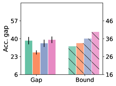
(a) ENZYMES

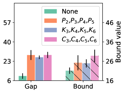
(b) PROTEINS

Figure 1: Accuracy gap and bound value using different homomorphism pattern sets, obtained from GCN of 4 layers.

7 Empirical Studies

Compute $\phi_{\#}^{\mathcal{F},L}\mu_{c}$ and $\phi_{\#}^{\mathcal{F},L}\nu_{c}$.

An intuitive choice of $\phi_{\#}^{\mathcal{F},L}\mu_{c}$ is the Lovász vector where each element in the vector is a homomorphism count of a pattern in $T_{L}(\mathcal{F})$. However, for GNNs listed in Section 4, the corresponding $T_{L}(\mathcal{F})$ is too large to compute the homomorphism counts explicitly: for 1-WL GNNs, $T_{L}(\mathcal{F})$ contains all trees up to depth $L$, for homomorphism-injected GNNs, $T_{L}(\mathcal{F})$ contains all $\mathcal{F}$-pattern trees up to depth $L$ (Barceló et al., 2021). Fortunately, we can use colour histograms obtained from the $\mathcal{F}$-WL (Barceló et al., 2021) algorithm as an equally expressive choice for $\phi_{\#}^{\mathcal{F},L}\mu_{c}$.

A colour histogram is essentially a vector representation of a graph, where each element is the count of the appearance of a particular node colour. The node-level $\phi_{\#}^{\mathcal{F},L}\nu_{c}$ can also be computed in this way, where a node is represented as a histogram of its neighbours’ node colours. We stack node colour counts of each iteration to form the final node representation. Details about colour histogram representation can be found in the well-known work of WL subtree graph kernel (Shervashidze et al., 2011).

Estimate KL Divergence.

The KL divergence in Lemma 5.3 and Lemma 5.6 measures the divergence of two sampled distributions. Because the distributions are multi-dimensional, we estimate the corresponding multivariate KL divergence according to Pérez-Cruz (2008).

7.1 Experiment Evaluation

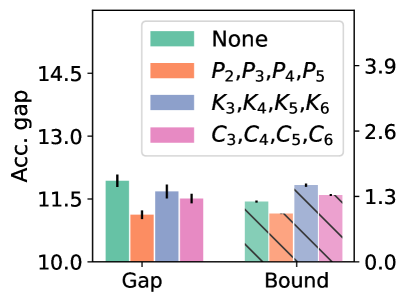
(a) PubMed: 4 layers

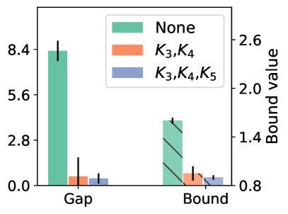
(b) PATTERN: 16 layers

Figure 2: Accuracy gap and bound value using different homomorphism pattern sets

We investigate how well the bounds align with observed generalization gap. In particular, we evaluate the generalization gaps of GCN on several datasets across node and graph classification tasks, with different numbers of layers and pattern sets, then compare the gaps with the proposed generalization bounds.

Tasks and Datasets

We evaluate graph and node classification tasks. For graph classification, we use ENZYMES, PROTEINS and PTC-MR from the TU datasets (Morris et al., 2020). Each dataset is randomly split into 90%/10% for training and test. For node classification, we evaluated the generalization gap on Cora, CiteSeer, and PubMed citation datasets (Sen et al., 2008; Yang et al., 2016), each of which is divided into 60% /40% for training and test. We use the differences in accuracy and loss between training and test as indicators of the generalization gap. We train 2,000 and 500 iterations for node and graph classification tasks, respectively. Each training is repeated five times to obtain mean accuracy and standard deviation. For node classification, we additionally evaluate the inductive setting on the PATTERN dataset (Dwivedi et al., 2023), which has over 12,000 artificially generated graphs resembling social networks or communities. The node classification task on PATTERN predicts whether a node belongs to a particular cluster or pattern. As shown by Barceló et al. (2021), classification accuracy is greatly improved on PATTERN after injecting homomorphism information.

Setup and Configuration

To calculate the bounds in Lemma 5.3 and Lemma 5.6, one needs to compute the ratio of Lipschitz constant and loss margin $\frac{L_{c}}{\gamma}$. As we focus on the upper-bound generalization gap, it is easier computationally to set the ratio to a “safe” constant. In practice, we set $\frac{L_{c}}{\gamma}$ to 3 and 6 for graph and node tasks respectively. The two numbers are “safe” because empirically they are larger than the ones estimated following the method used by Chuang et al. (2021). We use the largest pair-wise distance from the training set as the value of diameter in Lemma 5.3 and Lemma 5.6. We set $\delta$ to 0.01, so the computed bound is of high probability.

We use GCN (Kipf & Welling, 2017) as the base model and inspect how the bounds capture the trend of changes in generalization gaps w.r.t. (i) number of layers, and (ii) ingested homomorphism and subgraph counts .

7.2 Results and Discussion

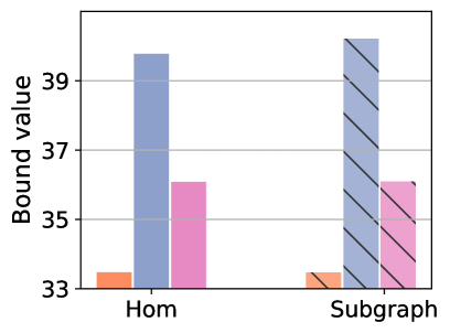
(a) ENZYMES

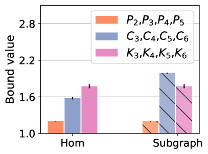
(b) PubMed

Figure 3: Bounds of homomorphism-injected and subgraph-injected models of 4 layers.

Layer		Dataset
		ENZYMES	PROTEINS	PTC-MR
1	Acc. gap	18.92±4.28	7.22±1.14	38.92±5.54
	Loss gap	0.69±0.06	0.11±0.00	1.03±0.12
	Bound	1.64±0.0.00	1.51±0.47	1.74±0.00
	# Histogram	586	929	200
2	Acc. gap	20.78±4.23	7.65±3.77	40.24±3.01
	Loss gap	0.64±0.08	0.10±0.01	0.95±0.09
	Bound	10.02±0.00	5.72±0.71	3.70±0.03
	# Histogram	595	996	257
3	Acc. gap	32.48±1.57	9.33±0.85	48.94±5.88
	Loss gap	0.89±0.06	0.15±0.15	1.25±0.14
	Bound	23.21±0.00	14.82±1.15	7.98±0.08
	# Histogram	595	996	258
4	Acc. gap	38.18±3.50	10.05±2.43	47.13±1.46
	Loss gap	1.12±0.07	0.21±0.03	1.48±0.25
	Bound	31.73±0.00	21.13±1.63	13.43±0.17
	# Histogram	595	996	258
5	Acc. gap	43.22±3.92	11.10±1.23	44.15±4.72
	Loss gap	1.28±0.21	0.28±0.04	1.61±0.20
	Bound	36.10±0.00	25.88±2.23	18.26±0.27
	# Histogram	595	996	258
6	Acc. gap	41.03±3.07	12.30±3.96	47.40±3.67
	Loss gap	1.38±0.14	0.32±0.07	1.60±0.04
	Bound	40.73±0.00	29.13±3.10	21.25±0.08
	# Histogram	595	996	258

Table 1: Graph classification accuracy and loss gap using different numbers of layers, compared with bound and number of colour histograms (graphs distinguishable by 1-WL).

Bound w.r.t Number of Layers.

As listed in Table 1 and Table 2, increasing layers increases both accuracy and loss gaps, as well as the generalization bound. We also listed the VC dimension bound proposed by Morris et al. (2023) in Table 1, which is essentially the number of graphs distinguishable by 1-WL (number of colour histograms). Compared with our bound, the VC bound cannot reflect generalization gap changes after the number of colour histograms stabilizes. For example, the number of colour histograms no longer changes after two layers for ENZYMES while the generalization gap continues to increase. Compared with the bounds in Liao et al. (2021); Garg et al. (2020) that are at least in the order of $10^{4}$, our bound is less vacuous as it matches the scale of the empirical gap.

Bound w.r.t Graph Patterns.

Beyond the vanilla GCN, we are interested in understanding if the proposed bound can reflect changes in the generalization gap w.r.t. different graph patterns that are used to inject homomorphism and subgraph counts. The evaluated HI-GNN corresponds to LGP-GNN (Barceló et al., 2021), the evaluated SI-GNN corresponds to a variant of GSN (Bouritsas et al., 2023) without dividing subgraph counts by the number of automorphisms. In Figure 1, we plot the accuracy gap vs generalization bound from three different pattern sets, compared with the vanilla GCN. We use $P_{n}$, $K_{n}$ and $C_{n}$ to denote n-path, n-clique and n-cycle graphs, respectively, and use “None” to denote vanilla GCN. We observe that different pattern sets cause different changes in the generalization gap. Namely, in ENZYMES, the path patterns lead to a smaller gap than cliques and cycle. Cycles lead to a larger gap than cliques. These changes in the generalization gap are also reflected in the corresponding bound, except for ENZYMES, where the gap for vanilla GCN is higher than others but the bound is lower. We also observe a similar trend in Figure 2 for node classification. We found that in cases where injecting homomorphism information reduces generalization gaps, the corresponding $\mathcal{F}$-WL algorithm requires fewer iterations than 1-WL to stabilise. This contributes to smaller diameter and KL divergence and further leads to smaller bounds.

Homomorphism vs Subgraph Counts.

Finally, we compare homomorphism-injected models with subgraph-injected models using the same pattern set, as shown in Figure 3. We note for cycles, subgraph counts tend to cause a higher bound value than homomorphism counts, while the two bound values are the same for paths and cliques. Recall a pattern $F$’s subgraph count can be derived from homomorphism counts of the corresponding $\operatorname{spasm}(F)$. This observation matches the expectation that, in general, subgraph counts have a larger entropy than homomorphism counts, thus results in a larger bound value. For cliques, the $\operatorname{spasm}$ of a clique only contains itself, i.e. the homomorphism count of a clique equals its subgraph count, so the bound value remains the same. For paths, the $\operatorname{spasm}$ of each path in $\{P_{2},P_{3},P_{4},P_{5}\}$ largely overlaps with the set itself $\{P_{2},P_{3},P_{4},P_{5}\}$, leading to a smaller variance and thus smaller bound value. For cycles, the $\operatorname{spasm}$ of each cycle contains paths of smaller size, and these paths do not overlap with the cycle set, leading to larger variance and entropy and, thus, a larger bound value.

Layer		Dataset
		Cora	CiteSeer	PubMed
1	Acc. gap	13.73±0.04	25.51±0.03	1.64±0.01
	Loss gap	0.48±0.00	1.12±0.01	0.03±0.00
	Bound	4.18±0.00	4.63±0.02	0.47±0.01
2	Acc. gap	13.41±0.19	28.16±0.21	4.46±0.20
	Loss gap	0.60±0.01	1.84±0.03	0.11±0.00
	Bound	4.57±0.00	4.63±0.02	0.55±0.02
3	Acc. gap	14.09±0.49	29.72±0.35	10.36±0.10
	Loss gap	0.98±0.04	2.83±0.12	0.34±0.00
	Bound	6.09±0.13	5.09±0.02	1.03±0.05
4	Acc. gap	14.39±0.34	30.48±0.13	11.93±1.47
	Loss gap	1.21±0.08	3.79±0.08	0.46±0.02
	Bound	6.97±0.14	5.73±0.03	1.45±0.02
5	Acc. gap	14.65±0.55	30.77±0.41	11.99±0.12
	Loss gap	1.62±0.12	5.15±0.22	0.52±0.02
	Bound	7.96±0.15	6.48±0.05	1.77±0.02
6	Acc. gap	14.96±0.68	30.22±0.41	11.90±0.25
	Loss gap	1.93±0.11	6.52±0.25	0.52±0.02
	Bound	7.96±0.15	7.24±0.06	1.77±0.02

Table 2: Node classification accuracy and loss gap using different numbers of layers, compared with bound value.

8 Conclusion

In this study, we delve into the generalization ability of GNNs by examining the entropy inherent in graph homomorphism, and integrating it with information-theoretic measures. This approach enables us to devise graph structure-aware generalization bounds that are useful for both graph and node classification tasks. These bounds, applicable to various GNNs within a unified homomorphism framework, closely match the actual generalization gaps observed in empirical evaluations on both real-world and synthetic datasets.

Impact Statement

This paper presents work whose goal is to advance the field of machine learning. There are many potential societal consequences of our work, none of which we feel must be specifically highlighted here.

Appendix A Notations

We list the notations used in Table 3.

$f_{\text{agg}}$, $f_{\text{upd}}$, $f_{\text{comb}}$ $f_{\operatorname{readout}}$	functions used in the aggregation, update, combine and readout steps of GNN
$h_{v}$, $h_{G}$	the vector representation of node $v$, graph $G$ resp.
$h_{\varphi}$	the vector representation of the homomorphism image under $\varphi$
$h_{F\rightarrow G}$	the aggregated representation of all homomorphism images from $F$ to $G$
$F$, $G$	graphs
$V_{G}$, $E_{G}$	the ndoe and edge sets of G
$\varphi:V_{F}\rightarrow V_{G}$	a homomorphism mapping from F to G
$\Phi_{F\rightarrow G}$	the set of all homomorphism mappings from $F$ to $G$
$\mathcal{F}$	a set of graph patterns
$F_{i}$	a unrooted pattern graph
$F^{r}_{i}$	a pattern graph rooted at node $r$
$\operatorname{hom}(F,G)$	the count of homomorphisms from $F$ to $G$
$\operatorname{Hom}(\mathcal{F},G)$	Lovász vector $\left(\operatorname{hom}(F_{1},G),\dots,\operatorname{hom}(F_{|\mathcal{F}|},G)\right)$
$X_{F\rightarrow G}$	a random variables representing a homomorphism mapping $\varphi$ uniformly chosen from $\Phi_{F\rightarrow G}$.
$X_{\mathcal{F}\rightarrow G}$	a collection of random variables $\left(X_{F_{1}\rightarrow G},\dots,X_{F_{|\mathcal{F}|}\rightarrow G}\right)$
$\mathrm{H}(X_{F\rightarrow G})$	the entropy of the random variable $X_{F\rightarrow G}$
$\mathrm{H}(X_{\mathcal{F}\rightarrow G})$	the joint entropy $\mathrm{H}(X_{F_{1}\rightarrow G},\dots,X_{F_{|\mathcal{F}|}\rightarrow G})$
$\operatorname{spasm}(G)$	the set of all homomorphic images of G
$\mathcal{W}_{p}(\mu,\nu)$	$p$-Wasserstein distance of two probability distributions $\mu$ and $\nu$
$\operatorname{TV}(\mu,\nu)$	total variation between two distributions $\mu$ and $\nu$
$\Delta(\mathcal{X})$	the diameter of the space $\mathcal{X}$
$D_{\text{KL}}(\mu\|\nu)$	KL-divergence of distributions $\mu$ and $\nu$
$\operatorname{Var}_{k,p}(\mu)$	Wasserstein-$p$ $k$-variance of the distribution $\mu$
$\operatorname{Var}_{k}(\mu)$	Wasserstein-$1$ $k$-variance of the distribution $\mu$
$\phi$, $\Theta$	a feature learner and its space
$f$, $\Psi$	a classifier and its function space
$\mathcal{Y}$	output space of a classifier of $K$ classes
$\mathcal{X}$	vector input space of a feature learner
$\rho_{f}(\cdot)$	a multi-class margin loss function of the classifier $f$
$\hat{R}_{\mu}(\cdot)$	expected population loss
$\hat{R}_{\gamma,m}(\cdot)$	$\gamma$-margin empirical loss on $m$ samples
$m$	the number of samples
$m_{c}$	the number of samples in class $c$
$\mu_{c}$, $\nu_{c}$	the marginal distribution of data in class $c$
$\phi_{\#}\mu$	the push-forward measure of the distribution $\mu$ w.r.t the feature learner $\phi$
$p$	the distribution of classes
$\operatorname{gen}(f\circ\phi)$	the generalization gap of a model compose of $f$ and $\phi$
$\operatorname{Lip}(\cdot)$	the margin Lipschitz constant of a function
$\operatorname{tw}(F)$	the tree width of $F$
$\operatorname{td}(F)$	the depth of the tree graph $F$
$\Delta(\cdot)$	diameter of a space
$T_{L}(\mathcal{F})$	the set of rooted $\mathcal{F}$-pattern trees of depth at most $L$
$\mathcal{F}_{\operatorname{hom}}$, $\mathcal{F}_{\operatorname{sub}}$	the set of homomorphism/subgraph patterns used by HI-GNN/SI-GNN

Table 3: Notatoin Table

Appendix B Additional Experiment Configuration

We follow the same setup from Morris et al. (2023); Tang & Liu (2023); Cong et al. (2021a) to remove regularizations including dropout and weight decay, and use the Adam optimizer. We use 64 as the inner dimension for intermediate layers. We have also run the experiments with 128 inner dimension and observed similar results. We train for 2000 and 500 iterations for node and graph tasks, both using 0.001 as the learning rate. We record the best accuracy and loss for both training and test set and report the difference.

Appendix C Missing Proofs

See 4.2

Proof.

We prove the above statements one by one.

• Given that $\mathcal{F}$ contains all graphs of treewidth up to $k$, the corresponding $\mathcal{F}$-pattern trees contain at least all graphs of treewidth up to $k$ too. Since the construction of $\mathcal{F}$-pattern trees does not increase treewidth, the maximum treewidth of the $\mathcal{F}$-pattern trees remains to be $k$. According to Dvorák (2010); Dell et al. (2018); Barceló et al. (2021), we know that HOM-GNN with $\mathcal{F}$ is equivalent in expressivity to k-WL GNN.

• It is easy to see that HOM-GNN and HI-GNN have the same form when $R^{v}=\{\!\!\{\varphi(u)|u\in V_{F^{v}}\}\!\!\}$.

• SI-GNN enriches node features using subgraph counts in the same way as HI-GNN using homomorphism counts. So it suffices to show that subgraph counts can be computed from homomorphism counts. Let the subgraph counts of $F$ in $G$ as $\operatorname{sub}(F,G)$. Curticapean et al. (2017) shows that $\operatorname{sub}(F,G)$ can be computed from a linear combination of $\operatorname{hom}(F_{i},G),\dots,\operatorname{hom}(F_{n},G)$, where $F_{i},\dots,F_{n}$ are the patterns in the $\operatorname{spasm}(F)$. Supposing that $f_{\text{agg}}$ is a universal learner such as MLP, the linear combination can be learned by $f_{\text{agg}}$. Thus, SI-GNN has the same expressivity as HOM-GNN with $\mathcal{F}=\operatorname{spasm}(\mathcal{F}_{\operatorname{sub}})$.

The proof is done.

∎

Before we prove the proposed bounds, we introduce a few definitions and theorems from previous works, as they are useful in the later proofs.

C.1 Margin Bound with Wasserstein Distance

Definition C.1 ($p$-Wasserstein Distance (Chuang et al., 2021)).

Let $\mu$ and $\nu\in\textsc{Prob}(\mathbb{R}^{d})$ be two probability measures. The $p$-Wasserstein distance with the Euclidean cost function $\parallel\cdot\parallel$ is defined as

$$\mathcal{W}_{p}(\mu,\nu):=\inf_{\pi\in\Pi(\mu,\nu)}\left(\mathbb{E}_{(x,y)\sim\pi}\parallel x-y\parallel^{p}\right)^{\frac{1}{p}}$$

where $\Pi(\mu,\nu)\subseteq\textsc{Prob}(\mathbb{R}^{d}\times\mathbb{R}^{d})$ denotes the set of all couplings measure whose marginals are $\mu$ and $\nu$, respectively.

Remark C.2.

Wasserstein distance measures the minimal cost to transport a distribution $\mu$ to a distribution $\nu$.

Definition C.3 (Wasserstein-$p$ $k$-variance (Solomon et al., 2022)).

Given a probability distribution $\mu\in\textsc{Prob}(\mathbb{R}^{d})$ and a parameter $k\in\mathbb{N}$, the Wasserstein-$p$ $k$-variance is defined as

$$\operatorname{Var}_{k,p}(\mu)=c_{p}(k,d)\cdot\mathbb{E}_{S,\tilde{S}\sim\mu^{k}}\left[\mathcal{W}^{p}_{p}(\mu_{S},\mu_{\tilde{S}})\right],$$

where $\mu_{S}$ and $\mu_{\tilde{S}}$ are empirical measures of the same size and $c_{p}(k,d)$ is a normalization term.

Remark C.4 (Wasserstein-$1$ $k$-variance).

In this work, we focus on the Wasserstein-1 $k$-variance:

$$\operatorname{Var}_{k}(\mu):=\mathbb{E}_{S,\tilde{S}\sim\mu^{k}}[\mathcal{W}_{1}(\mu_{S},\mu_{\tilde{S}})].$$

Chuang et al. (2021) studied generalization using Wasserstein distance and revealed that the concentration and separation of features play crucial roles in generalization.

Lemma C.5 (Chuang et al. (2021)).

Let $f=[f_{1},\dots,f_{K}]\in\Psi$ where $\Psi=\Psi_{1}\times\dots\times\Psi_{K}$, $f_{i}\in\Psi_{i}$, and $\Psi_{i}:\mathcal{X}\rightarrow\mathbb{R}$. Fix $\gamma>0$. Denote the generalization gap as $\operatorname{gen}(f\circ\phi)=R_{\mu}(f\circ\phi)-\hat{R}_{\gamma,m}(f\circ\phi)$. The following bound holds for all $f\in\Psi$ with probability at least $1-\delta>0$:

$$\operatorname{gen}(f\circ\phi)\leq \mathbb{E}_{c\sim\pi}\left[\frac{\operatorname{Lip}\left(\rho_{f}(\cdot,c)\right)}{\gamma}\operatorname{Var}_{m_{c}}\left(\phi_{\#}\mu_{c}\right)\right]$$

$$+\sqrt{\frac{\log(1/\delta)}{2m}},$$

where $\operatorname{Lip}\left(\rho_{f}(\cdot,c)\right)=\sup_{x,x^{\prime}\in\mathcal{X}}\frac{\left|\rho_{f}(\phi(x),c)-\rho_{f}\left(\phi\left(x^{\prime}\right),c\right)\right|}{\left\|\phi(x)-\phi\left(x^{\prime}\right)\right\|_{2}}$ is the margin Lipschitz constant w.r.t $\phi$.

C.2 Total Variation and KL-divergence

Definition C.6 (Total Variation).

The total variation between two distributions $\mu$ and $\nu$ on $\mathbb{R}^{d}$ is

$$\operatorname{TV}(\mu,\nu):=\sup_{A\in\mathbb{R}^{d}}\{\mu(A)-\nu(A)\}.$$

where $\mu(A)$ and $\nu(A)$ are the cumulative probabilities on $\mu$ and $\nu$ respectively over the set $A$.

Theorem C.7 (Theorem 6.15 (Villani et al., 2009)).

The 1-Wasserstein distance is dominated by the total variation, i.e. let $\mu$ and $\nu$ be two distributions on $\mathcal{M}\in\mathbb{R}^{d}$, $\Delta(\mathcal{M})$ be the diameter of $\mathcal{M}$, we have $\mathcal{W}_{1}(\mu,\nu)\leq\Delta(\mathcal{M})\operatorname{TV}(\mu,\nu)$.

Lemma C.8 (Pinsker’s and Bretagnolle–Huber’s (BH) inequalities (Polyanskiy & Wu, 2014)).

Let $\mu$ and $\nu$ be two probability distributions on $\mathcal{M}$, and $D_{\text{KL}}(\mu\|\nu)$ be the KL-divergence. Then

$$\operatorname{TV}(\mu,\nu)\leq\sqrt{\min(\frac{1}{2}D_{\text{KL}}(\mu\|\nu),1-\exp(-D_{\text{KL}}(\mu\|\nu)))}.$$

C.3 $\mathcal{F}$-pattern Trees and Homomorphism

We introduce Theorem 1 from Barceló et al. (2021).

Theorem C.9 (Theorem 1 of Barceló et al. (2021)).

For any finite collection $\mathcal{F}$ of patterns, vertices $v$ and $w$ in a graph $G$ $\operatorname{hom}(T^{r},G^{v})=\operatorname{hom}(T^{r},G^{w})$ for every rooted $\mathcal{F}$-pattern tree $T^{r}$. Similarly, $G$ and $H$ are undistinguishable by the $\mathcal{F}$-WL-test if and only if $\operatorname{hom}(T,G)=hom(T,H)$, for every (unrooted) $\mathcal{F}$-pattern tree.

Theorem C.9 is generalized to $\mathcal{F}$-WL of $L$ iterations by Barceló et al. (2021) in their proof.

Theorem C.10 (Proof of Theorem 1 in Barceló et al. (2021)).

For any finite collection $\mathcal{F}$ of patterns, graphs $G$ and $H$, vertices $v\in V_{G}$ and $w\in V_{H}$ and $L\geq 0$:

$$(G,v)\equiv^{(L)}_{\mathcal{F}\text{-WL}}(H,w)\Longleftrightarrow\operatorname{hom}(T^{r},G^{v})=\operatorname{hom}(T^{r},H^{w}),$$

for every $\mathcal{F}$-pattern tree $T^{r}$ of depth at most $L$. Similarly,

$$G\equiv^{(L)}_{\mathcal{F}\text{-WL}}H\Longleftrightarrow\operatorname{hom}(T,G)=\operatorname{hom}(T,H),$$

for every (unrooted) $\mathcal{F}$-pattern tree of depth at most $L$.

Now we prove the proposed bounds.

See 5.2

Proof.

Recall the bound in Lemma C.5,

$$\operatorname{gen}(f\circ\phi)\leq\mathbb{E}_{c\sim p}\left[\frac{L_{c}}{\gamma}\operatorname{Var}_{m_{c}}\left(\phi^{\mathcal{F},L}_{\#}\mu_{c}\right)\right]+\sqrt{\frac{\log(1/\delta)}{2m}}$$

Now we seek to bound $\operatorname{Var_{m_{c}}}(\phi_{\#}^{\mathcal{F},L}\mu_{c})$. By definition,

$$\operatorname{Var}_{m_{c}}(\phi_{\#}^{\mathcal{F},L}\mu_{c})=\mathbb{E}_{S,\tilde{S}\sim\mu_{c}^{m_{c}}}[\mathcal{W}_{1}(\phi_{\#}^{\mathcal{F},L}\mu_{S},\phi_{\#}^{\mathcal{F},L}\mu_{\tilde{S}})]$$

By Theorem C.7, we have

$$\mathcal{W}_{1}(\phi_{\#}^{\mathcal{F},L}\mu_{S},\phi_{\#}^{\mathcal{F},L}\mu_{\tilde{S}})\leq\beta_{c}\operatorname{TV}(\phi_{\#}^{\mathcal{F},L}\mu_{S},\phi_{\#}^{\mathcal{F},L}\mu_{\tilde{S}})$$

Further by Lemma C.8, we have

$$\operatorname{TV}(\phi_{\#}^{\mathcal{F},L}\mu_{S},\phi_{\#}^{\mathcal{F},L}\mu_{\tilde{S}})\leq\Omega\left(D_{KL}\left(\phi_{\#}^{\mathcal{F},L}\mu_{S},\phi_{\#}^{\mathcal{F},L}\mu_{\tilde{S}}\right)\right)$$

Under HOM-GNN, according to Theorem C.9 and Theorem C.10, $\phi_{\#}^{\mathcal{F},L}$ encode the same amount of information as Lovász vector, i.e. $\mathrm{H}(\phi_{\#}^{\mathcal{F},L}\mu_{S})=\mathrm{H}(X_{T_{L}(\mathcal{F})\rightarrow S})$ and $\mathrm{H}(\phi_{\#}^{\mathcal{F},L}\mu_{\tilde{S}})=\mathrm{H}(X_{T_{L}(\mathcal{F})\rightarrow\tilde{S}})$. We have

$$D_{KL} \left(\phi_{\#}^{\mathcal{F},L}\mu_{S},\phi_{\#}^{\mathcal{F},L}\mu_{\tilde{S}}\right)=$$

$$D_{KL}\left(X_{T_{L}(\mathcal{F})\rightarrow S}\parallel X_{T_{L}(\mathcal{F})\rightarrow\tilde{S}}\right)$$

According to the definition of KL divergence, we know

$$D_{KL} \left(X_{T_{L}(\mathcal{F})\rightarrow S}\parallel X_{T_{L}(\mathcal{F})\rightarrow\tilde{S}}\right)$$

$$=\mathrm{H}(X_{T_{L}(\mathcal{F})\rightarrow S},X_{T_{L}(\mathcal{F})\rightarrow\tilde{S}})-\mathrm{H}(\mathrm{X_{T_{L}(\mathcal{F})\rightarrow S})}$$

Because $\mathrm{H}(X_{T_{L}(\mathcal{F})\rightarrow S},X_{T_{L}(\mathcal{F})\rightarrow\tilde{S}})$ is a joint entropy, and $S$ and $\tilde{S}$ are independent because of 5.1, we have

$$\mathrm{H} (X_{T_{L}(\mathcal{F})\rightarrow S},X_{T_{L}(\mathcal{F})\rightarrow\tilde{S}})=$$

$$\mathrm{H}(X_{T_{L}(\mathcal{F})\rightarrow S})+\mathrm{H}(X_{T_{L}(\mathcal{F})\rightarrow\tilde{S}})$$

Hence,

$$D_{KL}\left(X_{T_{L}(\mathcal{F})\rightarrow S}\parallel X_{T_{L}(\mathcal{F})\rightarrow\tilde{S}}\right)\leq\mathrm{H}(\mathrm{X}_{T_{L}(\mathcal{F})\rightarrow\tilde{S}})$$

For simplicity of notation, we swap $\tilde{S}$ with $S$ and land on

$$\operatorname{gen}(f\circ\phi^{\mathcal{F},L})\leq$$

$$\mathbb{E}_{c\sim\pi}\left[\frac{L_{c}}{\gamma}\mathbb{E}_{S\sim\mu_{c}^{m_{c}}}\left[\beta_{c}\Omega\left(\mathrm{H}(X_{T_{L}(\mathcal{F})\rightarrow S})\right)\right]\right]+\sqrt{\frac{\log(2/\delta)}{2m}}$$

The proof is done.

∎

See 5.3

Proof.

Recall the bound in Lemma C.5,

$$\operatorname{gen}(f\circ\phi)\leq\mathbb{E}_{c\sim p}\left[\frac{L_{c}}{\gamma}\operatorname{Var}_{m_{c}}\left(\phi^{\mathcal{F},L}_{\#}\mu_{c}\right)\right]+\sqrt{\frac{\log(1/\delta)}{2m}}$$

Chuang et al. (2021) (Lemma 5) show the $k$-variance $\operatorname{Var}_{k}(\mu)$ can be estimated empirically by $\widehat{\operatorname{Var}}_{k,n}(\phi_{\#}^{\mathcal{F},L}\mu_{c})$,

$$\operatorname{Var}_{k}(\phi_{\#}^{\mathcal{F},L}\mu_{c})\leq\widehat{\operatorname{Var}}_{k,n}(\phi_{\#}^{\mathcal{F},L}\mu_{c})+\sqrt{\frac{2\beta_{c}^{2}\log(1/\delta)}{nk}}$$

where

$$\widehat{\operatorname{Var}}_{k,n}(\phi_{\#}^{\mathcal{F},L}\mu_{c})=\frac{1}{n}\sum_{j=1}^{n}\mathcal{W}_{1}(\phi_{\#}^{\mathcal{F},L}\mu_{S^{j}},\phi_{\#}^{\mathcal{F},L}\mu_{\tilde{S}^{j}})$$

$\widehat{\operatorname{Var}}_{k,n}(\phi_{\#}^{\mathcal{F},L}\mu_{c})$ can be computed using $n$ samples $\{S^{j},\tilde{S}^{j}\}^{n}_{j=1}$ where each $S^{j},\tilde{S}^{j}\sim\mu^{k}$. With probability at least $1-\delta$, for $m=\sum_{c=1}^{K}\lfloor\frac{m_{c}}{2n}\rfloor$, $\operatorname{gen}(f\circ\phi^{\mathcal{F},L})$ is bounded by

$$\mathbb{E}_{c\sim\pi} \left[\frac{L_{c}}{\gamma}\left(\widehat{\operatorname{Var}}_{\lfloor\frac{m_{c}}{2n}\rfloor,n}(\phi_{\#}^{\mathcal{F},L}\mu_{c})+2\beta_{c}\sqrt{\frac{\log(\frac{2K}{\delta})}{n\lfloor\frac{m_{c}}{2n}\rfloor}}\right)\right]$$

$$+\sqrt{\frac{\log(2/\delta)}{2m}}$$ (9)

Now we seek to upper bound the term $\mathcal{W}_{1}(\phi_{\#}^{\mathcal{F},L}\mu_{S^{j}},\phi_{\#}^{\mathcal{F},L}\mu_{\tilde{S}^{j}})$ in $\widehat{\operatorname{Var}}_{k,n}(\phi_{\#}^{\mathcal{F},L}\mu_{c})$ using KL divergence.

By Theorem C.7, we have

$$\mathcal{W}_{1}(\phi_{\#}^{\mathcal{F},L}\mu_{S^{j}},\phi_{\#}^{\mathcal{F},L}\mu_{\tilde{S}^{j}})\leq\beta_{c}\operatorname{TV}(\phi_{\#}^{\mathcal{F},L}\mu_{S^{j}},\phi_{\#}^{\mathcal{F},L}\mu_{\tilde{S}^{j}})$$

Further by Lemma C.8, we have

$$\operatorname{TV}(\phi_{\#}^{\mathcal{F},L}\mu_{S^{j}},\phi_{\#}^{\mathcal{F},L}\mu_{\tilde{S}^{j}})\leq\Omega\left(D_{KL}\left(\phi_{\#}^{\mathcal{F},L}\mu_{S^{j}},\phi_{\#}^{\mathcal{F},L}\mu_{\tilde{S}^{j}}\right)\right)$$

Putting together, we have

$$\widehat{\operatorname{Var}}_{k,n}(\phi_{\#}^{\mathcal{F},L}\mu_{c})\leq\frac{1}{n}\sum_{j=1}^{n}\left(\beta_{c}\Omega\left(D_{KL}(\phi_{\#}^{\mathcal{F},L}\mu_{S^{j}}\parallel\phi_{\#}^{\mathcal{F},L}\mu_{\tilde{S}^{j}})\right)\right)$$

Apply the inequality to Section C.3, then with probability at least $1-\delta>1$, we have $\operatorname{gen}(f\circ\phi^{\mathcal{F},L})$ is upper bounded by

$$\mathbb{E}_{c\sim\pi} \left[\frac{L_{c}}{\gamma}\left(\widetilde{D}_{KL}(\phi_{\#}^{\mathcal{F},L}\mu_{c})+2\beta_{c}\sqrt{\frac{\log(\frac{2K}{\delta})}{n\lfloor\frac{m_{c}}{2n}\rfloor}}\right)\right]$$

$$+\sqrt{\frac{\log(2/\delta)}{2m}}$$

The proof is done. ∎

See 5.5

Proof.

The proof is carried out in a similar way as Corollary 5.2. We consider patterns in $\mathcal{F}$ as rooted. Recall the bound in Lemma C.5,

$$\operatorname{gen}(f\circ\phi)\leq\mathbb{E}_{c\sim p}\left[\frac{L_{c}}{\gamma}\operatorname{Var}_{m_{c}}\left(\phi^{\mathcal{F},L}_{\#}\nu_{c}\right)\right]+\sqrt{\frac{\log(1/\delta)}{2m}}$$

Now we seek to bound $\operatorname{Var_{m_{c}}}(\phi_{\#}^{\mathcal{F},L}\nu_{c})$. By definition,

$$\operatorname{Var}_{m_{c}}(\phi_{\#}^{\mathcal{F},L}\nu_{c})=\mathbb{E}_{S,\tilde{S}\sim\nu_{c}^{m_{c}}}[\mathcal{W}_{1}(\phi_{\#}^{\mathcal{F},L}\nu_{S},\phi_{\#}^{\mathcal{F},L}\nu_{\tilde{S}})]$$

By Theorem C.7, we have

$$\mathcal{W}_{1}(\phi_{\#}^{\mathcal{F},L}\nu_{S},\phi_{\#}^{\mathcal{F},L}\nu_{\tilde{S}})\leq\beta_{c}\operatorname{TV}(\phi_{\#}^{\mathcal{F},L}\nu_{S},\phi_{\#}^{\mathcal{F},L}\nu_{\tilde{S}})$$

Further by Lemma C.8, we have

$$\operatorname{TV}(\phi_{\#}^{\mathcal{F},L}\nu_{S},\phi_{\#}^{\mathcal{F},L}\nu_{\tilde{S}})\leq\Omega\left(D_{KL}\left(\phi_{\#}^{\mathcal{F},L}\nu_{S},\phi_{\#}^{\mathcal{F},L}\nu_{\tilde{S}}\right)\right)$$

Under HOM-GNN, $\phi_{\#}^{\mathcal{F},L}$ encode the same information as Lovász vector for $N_{L}(S)$ and $N_{L}(\tilde{S})$, i.e. $\mathrm{H}(\phi_{\#}^{\mathcal{F},L}\nu_{S})=\mathrm{H}(X_{T_{L}(\mathcal{F})\rightarrow N_{L}(S)})$ and $\mathrm{H}(\phi_{\#}^{\mathcal{F},L}\nu_{\tilde{S}})=\mathrm{H}(X_{T_{L}(\mathcal{F})\rightarrow N_{L}(\tilde{S})})$ we have

$$D_{KL} \left(\phi_{\#}^{\mathcal{F},L}\nu_{S},\phi_{\#}^{\mathcal{F},L}\nu_{\tilde{S}}\right)=$$

$$D_{KL}\left(X_{T_{L}(\mathcal{F})\rightarrow N_{L}(S)}\parallel X_{T_{L}(\mathcal{F})\rightarrow N_{L}(\tilde{S})}\right)$$

According to the definition of KL divergence, we know

$$D_{KL}\left(X_{T_{L}(\mathcal{F})\rightarrow N_{L}(S)}\parallel X_{T_{L}(\mathcal{F})\rightarrow N_{L}(\tilde{S})}\right)$$

$$=\mathrm{H}(X_{T_{L}(\mathcal{F})\rightarrow N_{L}(S)},X_{T_{L}(\mathcal{F})\rightarrow N_{L}(\tilde{S})})-\mathrm{H}(\mathrm{X_{T_{L}(\mathcal{F})\rightarrow N_{L}(S)})}$$

Because $\mathrm{H}(X_{T_{L}(\mathcal{F})\rightarrow N_{L}(S)},X_{T_{L}(\mathcal{F})\rightarrow N_{L}(\tilde{S})})$ is a joint entropy, and $N_{L}(S)$ and $N_{L}(\tilde{S})$ are independent because of 5.4, we have

$$\mathrm{H} (X_{T_{L}(\mathcal{F})\rightarrow N_{L}(S)},X_{T_{L}(\mathcal{F})\rightarrow N_{L}(\tilde{S})})=$$

$$\mathrm{H}(X_{T_{L}(\mathcal{F})\rightarrow N_{L}(S)})+\mathrm{H}(X_{T_{L}(\mathcal{F})\rightarrow N_{L}(\tilde{S})})$$

Hence,

$$D_{KL} \left(X_{T_{L}(\mathcal{F})\rightarrow N_{L}(S)}\parallel X_{T_{L}(\mathcal{F})\rightarrow N_{L}(\tilde{S})}\right)$$

$$\leq\mathrm{H}(\mathrm{X}_{T_{L}(\mathcal{F})\rightarrow N_{L}(\tilde{S})})$$

For simplicity of notation, we swap $\tilde{S}$ with $S$ and land on

$$\operatorname{gen}(f\circ \phi^{\mathcal{F},L})\leq$$

$$\mathbb{E}_{c\sim\pi}\left[\frac{L_{c}}{\gamma}\mathbb{E}_{S\sim\nu_{c}^{m_{c}}}\left[\beta_{c}\Omega\left(\mathrm{H}(X_{T_{L}(\mathcal{F})\rightarrow N_{L}(S)})\right)\right]\right]$$

$$+\sqrt{\frac{\log(2/\delta)}{2m}}$$

The proof is done. ∎

See 5.6

Proof.

The proof is carried out in a similar way as Lemma 5.3. We consider patterns in $\mathcal{F}$ as rooted.

Recall the bound in Lemma C.5,

$$\operatorname{gen}(f\circ\phi)\leq\mathbb{E}_{c\sim p}\left[\frac{L_{c}}{\gamma}\operatorname{Var}_{m_{c}}\left(\phi^{\mathcal{F},L}_{\#}\nu_{c}\right)\right]+\sqrt{\frac{\log(1/\delta)}{2m}}$$

Chuang et al. (2021) (Lemma 5) show the $k$-variance $\operatorname{Var}_{k}(\nu)$ can be estimated empirically by $\widehat{\operatorname{Var}}_{k,n}(\phi_{\#}^{\mathcal{F},L}\nu_{c})$,

$$\operatorname{Var}_{k}(\phi_{\#}^{\mathcal{F},L}\nu_{c})\leq\widehat{\operatorname{Var}}_{k,n}(\phi_{\#}^{\mathcal{F},L}\nu_{c})+\sqrt{\frac{2\alpha_{c}^{2}\log(1/\delta)}{nk}}$$

where

$$\widehat{\operatorname{Var}}_{k,n}(\phi_{\#}^{\mathcal{F},L}\nu_{c})=\frac{1}{n}\sum_{j=1}^{n}\mathcal{W}_{1}(\phi_{\#}^{\mathcal{F},L}\nu_{S^{j}},\phi_{\#}^{\mathcal{F},L}\nu_{\tilde{S}^{j}})$$

$\widehat{\operatorname{Var}}_{k,n}(\phi_{\#}^{\mathcal{F},L}\nu_{c})$ can be computed using $n$ samples $\{S^{j},\tilde{S}^{j}\}^{n}_{j=1}$ where each $S^{j},\tilde{S}^{j}\sim\nu^{k}$. With probability at least $1-\delta$, for $m=\sum_{c=1}^{K}\lfloor\frac{m_{c}}{2n}\rfloor$, $\operatorname{gen}(f\circ\phi^{\mathcal{F},L})$ is bounded by

$$\mathbb{E}_{c\sim\pi} \left[\frac{L_{c}}{\gamma}\left(\widehat{\operatorname{Var}}_{\lfloor\frac{m_{c}}{2n}\rfloor,n}(\phi_{\#}^{\mathcal{F},L}\nu_{c})+2\alpha_{c}\sqrt{\frac{\log(\frac{2K}{\delta})}{n\lfloor\frac{m_{c}}{2n}\rfloor}}\right)\right]$$

$$+\sqrt{\frac{\log(2/\delta)}{2m}}$$ (10)

Now we seek to upper bound the term $\mathcal{W}_{1}(\phi_{\#}^{\mathcal{F},L}\nu_{S^{j}},\phi_{\#}^{\mathcal{F},L}\nu_{\tilde{S}^{j}})$ in $\widehat{\operatorname{Var}}_{k,n}(\phi_{\#}^{\mathcal{F},L}\nu_{c})$ using KL divergence.

By Theorem C.7, we have

$$\mathcal{W}_{1}(\phi_{\#}^{\mathcal{F},L}\nu_{S^{j}},\phi_{\#}^{\mathcal{F},L}\nu_{\tilde{S}^{j}})\leq\alpha_{c}\operatorname{TV}(\phi_{\#}^{\mathcal{F},L}\nu_{S^{j}},\phi_{\#}^{\mathcal{F},L}\nu_{\tilde{S}^{j}})$$

Further by Lemma C.8, we have

$$\operatorname{TV}(\phi_{\#}^{\mathcal{F},L}\nu_{S^{j}},\phi_{\#}^{\mathcal{F},L}\nu_{\tilde{S}^{j}})\leq\Omega\left(D_{KL}\left(\phi_{\#}^{\mathcal{F},L}\nu_{S^{j}},\phi_{\#}^{\mathcal{F},L}\nu_{\tilde{S}^{j}}\right)\right)$$

Putting together, we have

$$\widehat{\operatorname{Var}}_{k,n}(\phi_{\#}^{\mathcal{F},L}\nu_{c})\leq\frac{1}{n}\sum_{j=1}^{n}\left(\alpha_{c}\Omega\left(D_{KL}(\phi_{\#}^{\mathcal{F},L}\nu_{S^{j}}\parallel\phi_{\#}^{\mathcal{F},L}\nu_{\tilde{S}^{j}})\right)\right)$$

Apply the inequality to Section C.3, then with probability at least $1-\delta>1$, we have $\operatorname{gen}(f\circ\phi^{\mathcal{F},L})$ is upper bounded by

$$\mathbb{E}_{c\sim\pi} \left[\frac{L_{c}}{\gamma}\left(\widetilde{D}_{KL}(\phi_{\#}^{\mathcal{F},L}\nu_{c})+2\alpha_{c}\sqrt{\frac{\log(\frac{2K}{\delta})}{n\lfloor\frac{m_{c}}{2n}\rfloor}}\right)\right]$$

$$+\sqrt{\frac{\log(2/\delta)}{2m}}$$

The proof is done. ∎

See 6.2

Proof.

We prove the bullet points one by one.

1. We look at the two control factor of the bound separately: $\mathrm{H}(X_{T_{L}(\mathcal{F})\rightarrow S})$ and $\beta_{c}$. Barceló et al. (2021) shows that a $\mathcal{F}$-WL is run for $L$ rounds corresponds to the $\mathcal{F}$-pattern trees of depth $L$. So $|T_{L}(\mathcal{F})|$ grows with $L$. As discussed in Section 6, larger $|T_{L}(\mathcal{F})|$ does not necessarily result in a larger $X_{T_{L}(\mathcal{F})\rightarrow S}$, but $X_{T_{L}(\mathcal{F})\rightarrow S}$ does not decrease on $|T_{L}(\mathcal{F}|$. Now we look at $\beta_{c}$, given $\beta_{c}$ captures the diameter of $\phi^{\mathcal{F},L}_{\#}\mu_{c}$, larger $\beta_{c}$ at $L+1$ is larger or equal to $\beta_{c}$ at $L$. So the bound described in Corollary 5.2, at layer $L+1$, is larger or equal to the bound at layer $L$.

2. This bullet point can be proved in a similar way as the first bullet point.

3. It is easy to see that when $\mathcal{F}_{\operatorname{hom}}=\{\leavevmode\hbox to3.23pt{\vbox to3.23pt{\text{[drawing]}}}\}$, HOM-GNN is equivalent to 1-WL GNN, since $T_{L}(\{\leavevmode\hbox to3.23pt{\vbox to3.23pt{\text{[drawing]}}})$ contains all trees up to depth $L$ (Barceló et al., 2021). So when $\mathcal{F}$ has more patterns, $T_{L}(\mathcal{F})$ becomes larger. As a result, the bound value becomes higher.

4. From Corollary 4.2, we know $\mathcal{F}$ is a infinite set of graphs up to treewidth $k$. It is easy to see the set of $\mathcal{F}$-pattern trees of SI-GNN and HI-GNN , where each pattern has bounded treewidth up to $K$, is a subset of the $\mathcal{F}$-pattern tree for a k-WL GNN. So we know k-WL GNN has a higher bound value than SI-GNN and HI-GNN.

∎

References

- Arora et al. (2018) Arora, S., Ge, R., Neyshabur, B., and Zhang, Y. Stronger generalization bounds for deep nets via a compression approach. In Proceedings of the 35th International Conference on Machine Learning, volume 80, pp. 254–263, 2018.
- Barceló et al. (2021) Barceló, P., Geerts, F., Reutter, J., and Ryschkov, M. Graph neural networks with local graph parameters. Advances in Neural Information Processing Systems, 34:25280–25293, 2021.
- Bartlett & Mendelson (2002) Bartlett, P. L. and Mendelson, S. Rademacher and gaussian complexities: Risk bounds and structural results. Journal of Machine Learning Research, 3(Nov):463–482, 2002.
- Bevilacqua et al. (2022) Bevilacqua, B., Frasca, F., Lim, D., Srinivasan, B., Cai, C., Balamurugan, G., Bronstein, M. M., and Maron, H. Equivariant subgraph aggregation networks. In International Conference on Learning Representations, 2022.
- Blumer et al. (1989) Blumer, A., Haussler, D., and Warmuth, M. K. Learnability and the vapnik-chervonenkis dimension. Journal of the ACM (JACM), 36(4):929–965, 1989.
- Bouritsas et al. (2023) Bouritsas, G., Frasca, F., Zafeiriou, S., and Bronstein, M. M. Improving graph neural network expressivity via subgraph isomorphism counting. IEEE Trans. Pattern Anal. Mach. Intell., 45(1):657–668, 2023.
- Cai et al. (1992) Cai, J.-Y., Fürer, M., and Immerman, N. An optimal lower bound on the number of variables for graph identification. Combinatorica, 12(4):389–410, 1992.
- Camuto et al. (2021) Camuto, A., Deligiannidis, G., Erdogdu, M. A., Gürbüzbalaban, M., Simsekli, U., and Zhu, L. Fractal structure and generalization properties of stochastic optimization algorithms. In Advances in Neural Information Processing Systems, pp. 18774–18788, 2021.
- Chiang et al. (2023) Chiang, P., Ni, R., Miller, D. Y., Bansal, A., Geiping, J., Goldblum, M., and Goldstein, T. Loss landscapes are all you need: Neural network generalization can be explained without the implicit bias of gradient descent. In International Conference on Learning Representations, 2023.
- Chuang et al. (2021) Chuang, C.-Y., Mroueh, Y., Greenewald, K. H., Torralba, A., and Jegelka, S. Measuring generalization with optimal transport. Advances in Neural Information Processing Systems, 2021.
- Chung et al. (1986) Chung, F. R. K., Graham, R. L., Frankl, P., and Shearer, J. B. Some intersection theorems for ordered sets and graphs. J. Comb. Theory, Ser. A, 43(1):23–37, 1986.
- Cong et al. (2021a) Cong, W., Ramezani, M., and Mahdavi, M. On provable benefits of depth in training graph convolutional networks. In Advances in Neural Information Processing Systems, pp. 9936–9949, 2021a.
- Cong et al. (2021b) Cong, W., Ramezani, M., and Mahdavi, M. On provable benefits of depth in training graph convolutional networks. Advances in Neural Information Processing Systems, 34:9936–9949, 2021b.
- Costa & Grave (2010) Costa, F. and Grave, K. D. Fast neighborhood subgraph pairwise distance kernel. In International Conference on Machine Learning, pp. 255–262, 2010.
- Curticapean et al. (2017) Curticapean, R., Dell, H., and Marx, D. Homomorphisms are a good basis for counting small subgraphs. In Symposium on Theory of Computing, pp. 210–223, 2017.
- Dell et al. (2018) Dell, H., Grohe, M., and Rattan, G. Lovász meets weisfeiler and leman. In International Colloquium on Automata, Languages, and Programming, 2018.
- Dupuis et al. (2023) Dupuis, B., Deligiannidis, G., and Simsekli, U. Generalization bounds using data-dependent fractal dimensions. In International Conference on Machine Learning, volume 202, pp. 8922–8968, 2023.
- Dvorák (2010) Dvorák, Z. On recognizing graphs by numbers of homomorphisms. J. Graph Theory, 64(4):330–342, 2010.
- Dwivedi et al. (2023) Dwivedi, V. P., Joshi, C. K., Luu, A. T., Laurent, T., Bengio, Y., and Bresson, X. Benchmarking graph neural networks. J. Mach. Learn. Res., 24:43:1–43:48, 2023.
- Dziugaite & Roy (2018) Dziugaite, G. K. and Roy, D. M. Data-dependent pac-bayes priors via differential privacy. In Advances in Neural Information Processing Systems, pp. 8440–8450, 2018.
- Esser et al. (2021) Esser, P. M., Vankadara, L. C., and Ghoshdastidar, D. Learning theory can (sometimes) explain generalisation in graph neural networks. In Annual Conference on Neural Information Processing Systems, pp. 27043–27056, 2021.
- Gálvez et al. (2021) Gálvez, B. R., Bassi, G., Thobaben, R., and Skoglund, M. Tighter expected generalization error bounds via wasserstein distance. In Advances in Neural Information Processing Systems, pp. 19109–19121, 2021.
- Garg et al. (2020) Garg, V. K., Jegelka, S., and Jaakkola, T. S. Generalization and representational limits of graph neural networks. In International Conference on Machine Learning, volume 119, pp. 3419–3430, 2020.
- Horváth et al. (2004) Horváth, T., Gärtner, T., and Wrobel, S. Cyclic pattern kernels for predictive graph mining. In International Conference on Knowledge Discovery and Data Mining, pp. 158–167, 2004.
- Ju et al. (2023) Ju, H., Li, D., Sharma, A., and Zhang, H. R. Generalization in graph neural networks: Improved pac-bayesian bounds on graph diffusion. In International Conference on Artificial Intelligence and Statistics, volume 206, pp. 6314–6341, 2023.
- Kawaguchi et al. (2022) Kawaguchi, K., Deng, Z., Luh, K., and Huang, J. Robustness implies generalization via data-dependent generalization bounds. In International Conference on Machine Learning, volume 162, pp. 10866–10894, 2022.
- Kipf & Welling (2017) Kipf, T. N. and Welling, M. Semi-supervised classification with graph convolutional networks. In International Conference on Learning Representations, 2017.
- Li et al. (2022) Li, H., Wang, M., Liu, S., Chen, P.-Y., and Xiong, J. Generalization guarantee of training graph convolutional networks with graph topology sampling. In International Conference on Machine Learning, volume 162, pp. 13014–13051, 2022.
- Liao et al. (2021) Liao, R., Urtasun, R., and Zemel, R. S. A pac-bayesian approach to generalization bounds for graph neural networks. In International Conference on Learning Representations, 2021.
- Lovász (2012) Lovász, L. Large Networks and Graph Limits, volume 60 of Colloquium Publications. American Mathematical Society, 2012. ISBN 978-0-8218-9085-1.
- Maron et al. (2019) Maron, H., Ben-Hamu, H., Serviansky, H., and Lipman, Y. Provably powerful graph networks. In Advances in Neural Information Processing Systems, volume 32, 2019.
- Maskey et al. (2022) Maskey, S., Levie, R., Lee, Y., and Kutyniok, G. Generalization analysis of message passing neural networks on large random graphs. In Advances in Neural Information Processing Systems, 2022.
- Morris et al. (2019a) Morris, C., Ritzert, M., Fey, M., Hamilton, W. L., Lenssen, J. E., Rattan, G., and Grohe, M. Weisfeiler and leman go neural: Higher-order graph neural networks. In AAAI Conference on Artificial Intelligence, pp. 4602–4609, 2019a.
- Morris et al. (2019b) Morris, C., Ritzert, M., Fey, M., Hamilton, W. L., Lenssen, J. E., Rattan, G., and Grohe, M. Weisfeiler and leman go neural: Higher-order graph neural networks. In AAAI Conference on Artificial Intelligence, volume 33, pp. 4602–4609, 2019b.
- Morris et al. (2020) Morris, C., Kriege, N. M., Bause, F., Kersting, K., Mutzel, P., and Neumann, M. Tudataset: A collection of benchmark datasets for learning with graphs. In ICML 2020 Workshop on Graph Representation Learning and Beyond (GRL+ 2020), 2020.
- Morris et al. (2023) Morris, C., Geerts, F., Tönshoff, J., and Grohe, M. WL meet VC. In International Conference on Machine Learning, volume 202, pp. 25275–25302, 2023.
- Nguyen & Maehara (2020) Nguyen, H. and Maehara, T. Graph homomorphism convolution. In International Conference on Machine Learning, volume 119, pp. 7306–7316, 2020.
- Oono & Suzuki (2020) Oono, K. and Suzuki, T. Optimization and generalization analysis of transduction through gradient boosting and application to multi-scale graph neural networks. Advances in Neural Information Processing Systems, 33, 2020.
- Pérez-Cruz (2008) Pérez-Cruz, F. Kullback-leibler divergence estimation of continuous distributions. In 2008 IEEE International Symposium on Information Theory, ISIT, pp. 1666–1670, 2008.
- Polyanskiy & Wu (2014) Polyanskiy, Y. and Wu, Y. Lecture notes on information theory. Lecture Notes for ECE563 (UIUC) and, 6(2012-2016):7, 2014.
- Scarselli et al. (2018) Scarselli, F., Tsoi, A. C., and Hagenbuchner, M. The vapnik-chervonenkis dimension of graph and recursive neural networks. Neural Networks, 108:248–259, 2018.
- Sefidgaran et al. (2022) Sefidgaran, M., Chor, R., and Zaidi, A. Rate-distortion theoretic bounds on generalization error for distributed learning. In Advances in Neural Information Processing Systems, 2022.
- Sen et al. (2008) Sen, P., Namata, G., Bilgic, M., Getoor, L., Gallagher, B., and Eliassi-Rad, T. Collective classification in network data. AI Mag., 29(3):93–106, 2008.
- Shervashidze et al. (2011) Shervashidze, N., Schweitzer, P., Van Leeuwen, E. J., Mehlhorn, K., and Borgwardt, K. M. Weisfeiler-lehman graph kernels. Journal of Machine Learning Research, 12(9), 2011.
- Solomon et al. (2022) Solomon, J., Greenewald, K. H., and Nagaraja, H. N. $k$-variance: A clustered notion of variance. SIAM J. Math. Data Sci., 4(3):957–978, 2022.
- Tang & Liu (2023) Tang, H. and Liu, Y. Towards understanding the generalization of graph neural networks. In International Conference on Machine Learning, 2023.
- Thiede et al. (2021) Thiede, E. H., Zhou, W., and Kondor, R. Autobahn: Automorphism-based graph neural nets. In Annual Conference on Neural Information Processing Systems, pp. 29922–29934, 2021.
- Verma & Zhang (2019) Verma, S. and Zhang, Z. Stability and generalization of graph convolutional neural networks. In International Conference on Knowledge Discovery & Data Mining, pp. 1539–1548, 2019.
- Villani et al. (2009) Villani, C. et al. Optimal transport: old and new, volume 338. Springer, 2009.
- Wang et al. (2023) Wang, Q., Chen, D., Wijesinghe, A., Li, S., and Farhan, M. N-wl: A new hierarchy of expressivity for graph neural networks. In International Conference on Learning Representations, 2023.
- Weisfeiler & Leman (1968) Weisfeiler, B. and Leman, A. The reduction of a graph to canonical form and the algebra which appears therein. Nauchno-Technicheskaya Informatsia, 2:12–16, 1968.
- Welke et al. (2023) Welke, P., Thiessen, M., Jogl, F., and Gärtner, T. Expectation-complete graph representations with homomorphisms. In International Conference on Machine Learning, 2023.
- Wijesinghe & Wang (2022) Wijesinghe, A. and Wang, Q. A new perspective on ”how graph neural networks go beyond weisfeiler-lehman?”. In International Conference on Learning Representations, 2022.
- Wu et al. (2022) Wu, Q., Zhang, H., Yan, J., and Wipf, D. P. Handling distribution shifts on graphs: An invariance perspective. In International Conference on Learning Representations, 2022.
- Xu et al. (2019) Xu, K., Hu, W., Leskovec, J., and Jegelka, S. How powerful are graph neural networks? In International Conference on Learning Representations, 2019.
- Yang et al. (2016) Yang, Z., Cohen, W. W., and Salakhutdinov, R. Revisiting semi-supervised learning with graph embeddings. In Proceedings of the 33nd International Conference on Machine Learning, volume 48, pp. 40–48, 2016.
- Zhang et al. (2023) Zhang, B., Feng, G., Du, Y., He, D., and Wang, L. A complete expressiveness hierarchy for subgraph GNNs via subgraph Weisfeiler-Lehman tests. In International Conference on Machine Learning, 2023.
- Zhang et al. (2017) Zhang, C., Bengio, S., Hardt, M., Recht, B., and Vinyals, O. Understanding deep learning requires rethinking generalization. In International Conference on Learning Representations, 2017.
- Zhang & Li (2021) Zhang, M. and Li, P. Nested graph neural networks. In Advances in Neural Information Processing Systems, pp. 15734–15747, 2021.
- Zhang et al. (2020) Zhang, S., Wang, M., Liu, S., Chen, P.-Y., and Xiong, J. Fast learning of graph neural networks with guaranteed generalizability: one-hidden-layer case. In International Conference on Machine Learning, 2020.
- Zhao et al. (2022) Zhao, L., Jin, W., Akoglu, L., and Shah, N. From stars to subgraphs: Uplifting any GNN with local structure awareness. In International Conference on Learning Representations, 2022.
- Zhou & Wang (2021) Zhou, X. and Wang, H. The generalization error of graph convolutional networks may enlarge with more layers. Neurocomputing, 424:97–106, 2021.