Implicit Image-to-Image Schrödinger Bridge for CT Super-Resolution and Denoising

Abstract

Conditional diffusion models have gained recognition for their effectiveness in image restoration tasks, yet their iterative denoising process, starting from Gaussian noise, often leads to slow inference speeds. As a promising alternative, the Image-to-Image Schrödinger Bridge (I²SB) initializes the generative process from corrupted images and integrates training techniques from conditional diffusion models. In this study, we extended the I²SB method by introducing the Implicit Image-to-Image Schrödinger Bridge (I³SB), transitioning its generative process to a non-Markovian process by incorporating corrupted images in each generative step. This enhancement empowers I³SB to generate images with better texture restoration using a small number of generative steps. The proposed method was validated on CT super-resolution and denoising tasks and outperformed existing methods, including the conditional denoising diffusion probabilistic model (cDDPM) and I²SB, in both visual quality and quantitative metrics. These findings underscore the potential of I³SB in improving medical image restoration by providing fast and accurate generative modeling.

1 Introduction

Restoration of high-quality images accurately from corrupted inputs is a common and challenging task in medical imaging processing such as denoising and super-resolution. In recent years, conditional diffusion models[10, 12] have demonstrated promising performance in tackling this task. Based on stochastic process theories, diffusion models provide a more stable solution to sample from complex distributions compared to Generative Adversarial Networks (GANs)[14]. However, diffusion models suffer from slow inference speed due to the large number of iterative denoising steps required to generate clean images starting from pure Gaussian noise.

Instead of starting from Gaussian noise, Schrödinger bridges[2, 3, 5] establish diffusion bridges between the distributions of clean and corrupted images. By initiating the diffusion process with the corrupted image that is closer to the clean one compared to Gaussian noise, Schrödinger bridges provide a promising approach to generate high-quality conditional samples with fewer diffusion steps. As a special case, the Image-to-Image Schrödinger Bridge (I²SB)[11] models the diffusion bridge between paired clean-corrupted samples, and enables efficient training through connecting it with the standard score-based diffusion model. Despite the reduction of the needed sampling steps compared to conventional diffusion models, it has been observed that I²SB tends to produce smoothed images[4] using small number of sampling steps, due to the so-called "regression to the mean effect"[6].

Inspired by the success of introducing non-Markovian process into the denoising diffusion probabilistic model (DDPM)[8] to formulate the denoising diffusion implicit model (DDIM)[13], we proposed a novel method, Implicit Image-to-Image Schrödinger Bridge (I³SB), which uses non-Markovian process during the inference of I²SB. The training process of the proposed I³SB is same with I²SB, but during testing, the initial corrupted image is incorporated in each step besides the current image and the estimated mean. A single parameter was proposed to balance between the Markovian (I²SB) and the non-Markovian (I³SB) components, which can be adjusted across the diffusion process for better image restoration. We validated the method on two image restoration tasks, including quarter-dose abdominal CT image denoising and 4$\times$ chest CT super-resolution. The proposed I³SB was compared to I²SB and conditional DDPM (cDDPM) and demonstrated improved texture restoration.

2 Method

Notation: Let $X_{t}\in R^{d}$ represent a d-dimensional stochastic process indexed by $t\in\left[0,1\right]$, and $N$ denote the number of generative steps. We denote the discrete generative time steps as $0=t_{0}<\cdots t_{n}\cdots<t_{N}=1$, and shorthand $X_{n}\equiv X_{t_{n}}$.

2.1 Image-to-Image Schrödinger Bridge

The I²SB establishes direct diffusion bridges between the clean image distribution $A$ and the corrupted image distribution $B$. Assuming paired data can be obtained during training, with $X_{0}$ denoting the sample from distribution $A$ and $X_{1}$ denoting the corresponding sample from distribution $B$, $X_{t}$ is designed to follow the distribution $q\left(X_{t}|X_{0},X_{1}\right)$:

$$q\left(X_{t}|X_{0},X_{1}\right)=\mathcal{N}\left(X_{t};\frac{\overline{\sigma}_{t}^{2}}{\overline{\sigma}_{t}^{2}+\sigma_{t}^{2}}X_{0}+\frac{{\sigma}_{t}^{2}}{\overline{\sigma}_{t}^{2}+\sigma_{t}^{2}}X_{1},\frac{{\sigma}_{t}^{2}\overline{\sigma}_{t}^{2}}{\overline{\sigma}_{t}^{2}+\sigma_{t}^{2}}I\right),$$ (1)

where ${\sigma}_{t}^{2}=\int_{0}^{t}\beta_{\tau}d\tau$ and $\overline{\sigma}_{t}^{2}=\int_{t}^{1}\beta_{\tau}d\tau$ represent variances accumulated from either side, and $\beta$ determines the speed of diffusion. As $X_{t}$ can be sampled analytically using equation (1), the network $\epsilon_{\theta}$ can be efficiently trained to predict the difference between $X_{t}$ and $X_{0}$ by minimizing the loss function:

$$\theta^{*}=\arg\min_{\theta}E_{X_{0},X_{1},y}E_{t\sim\mathcal{U}[0,1],X_{t}\sim q\left(X_{t}|X_{0},X_{1}\right)}\|\epsilon_{\theta}\left(X_{t},t,y\right)-\frac{X_{t}-X_{0}}{\sigma_{t}}\|,$$ (2)

where $y$ denotes any potential conditions.

In the generative process, I²SB begins with the corrupted image $X_{N}$ and iteratively approaches the clean image $X_{0}$. In the step from $X_{n+1}$ to $X_{n}$, $\hat{X}_{0}$, an approximation of $X_{0}$, is first calculated using the trained network $\epsilon_{\theta^{*}}$ and $X_{n+1}$:

$$\hat{X}_{0}=X_{n+1}-\sigma_{n+1}\epsilon_{\theta^{*}}\left(X_{n+1},t_{n+1},y\right),$$ (3)

where we use $\sigma_{n}\equiv\sigma_{t_{n}}$. Subsequently, $X_{n}$ is sampled from the DDPM posterior $p$ using $\hat{X}_{0}$ and $X_{n+1}$:

$$X_{n}\sim p\left(X_{n}|\hat{X}_{0},X_{n+1}\right).$$ (4)

Here, the DDPM posterior $p$ is expressed as

$$p\left(X_{n}|X_{0},X_{n+1}\right)=\mathcal{N}\left(X_{n};\frac{\alpha_{n}^{2}}{\alpha_{n}^{2}+\sigma_{n}^{2}}X_{0}+\frac{\sigma_{n}^{2}}{\alpha_{n}^{2}+\sigma_{n}^{2}}X_{n+1},\frac{\sigma_{n}^{2}\alpha_{n}^{2}}{\alpha_{n}^{2}+\sigma_{n}^{2}}I\right),$$ (5)

where $\alpha_{n}^{2}=\int_{t_{n}}^{t_{n+1}}\beta_{\tau}d\tau$ denotes the accumulated variance between consecutive time steps $t_{n}$ and $t_{n+1}$. The DDPM posterior $p$ satisfies the equation

$$q\left(X_{n}|X_{0},X_{N}\right)=\int p\left(X_{n}|X_{0},X_{n+1}\right)q\left(X_{n+1}|X_{0},X_{N}\right)dX_{n+1},$$ (6)

which guarantees that $X_{n}$ sampled using equation (4) is exactly a sample from $q\left(X_{n}|X_{0},X_{N}\right)$ assuming the trained network $\epsilon_{\theta^{*}}$ is perfect.

2.2 Implicit Image-to-Image Schrödinger Bridge

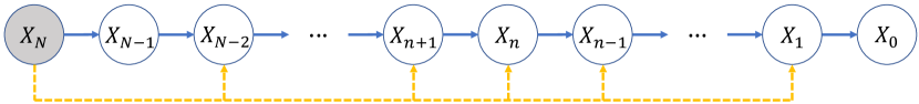
Figure 1: Non-Markovian generative process of I³SB. Solid arrows denote original dependencies in I²SB, and dotted arrows signify additional dependencies in I³SB.

Algorithm 1 Generation Procedures of I³SB

0:  $N$, $\left\{t_{n}\right\}$, $X_{N}\sim p_{B}\left(X_{N}\right)$, condition $y$, trained network $\epsilon_{\theta^{*}}$

  for $n=N$ to $1$ do

     Predict $\hat{X}_{0}$ using $\epsilon_{\theta^{*}}\left(X_{n},t_{n},y\right)$

     if $n==N$ then

        Sample $X_{n-1}$ from $p\left(X_{n-1}|\hat{X}_{0},X_{n}\right)$

     else if $1<n<N$ then

        Sample $X_{n-1}$ from $p_{G}\left(X_{n-1}|\hat{X}_{0},X_{n},X_{N}\right)$

     else

        $X_{0}=\hat{X}_{0}$

     end if

  end for

  return  $X_{0}$

We preserve the training process of I²SB and modify its generative process in our proposed I³SB. The generative process of I²SB is essentially a Markovian process, as $X_{n}$ is solely dependent on $X_{n+1}$ given the trained network $\epsilon_{\theta^{*}}$ and the condition $y$ ($\hat{X}_{0}$ is also a function of $X_{n+1}$). I³SB is non-Markovian by conditioning $X_{n}$ on both $X_{n+1}$ and $X_{N}$, as shown in Fig. 1. In the generative step from $X_{n+1}$ to $X_{n}$, we first compute $\hat{X}_{0}$ using equation (3) and then sample $X_{n}$ from the distribution $p_{G}$:

$$X_{n}\sim p_{G}\left(X_{n}|\hat{X}_{0},X_{n+1},X_{N}\right),$$ (7)

where $X_{N}$ is included. $p_{G}$ should satisfy the equation:

$$q\left(X_{n}|X_{0},X_{N}\right)=\int p_{G}\left(X_{n}|X_{0},X_{n+1},X_{N}\right)q\left(X_{n+1}|X_{0},X_{N}\right)dX_{n+1},$$ (8)

to guarantee that $X_{n}$ sampled using equation (7) is precisely a sample from $q\left(X_{n}|X_{0},X_{N}\right)$ assuming the trained network $\epsilon_{\theta^{*}}$ is perfect. Assuming that $p_{G}$ is a Gaussian distribution with a linear combination of $X_{0}$, $X_{n+1}$ and $X_{N}$ as its mean, $p_{G}$ can be expressed as

$$p_{G}\left(X_{n}|X_{0},X_{n+1},X_{N}\right)=\mathcal{N}\left(X_{n};A_{n}X_{0}+B_{n}X_{n+1}+C_{n}X_{N},g_{n}^{2}I\right),$$ (9)

where $A_{n}$, $B_{n}$ and $C_{n}$ represent the weights of $X_{0}$, $X_{n+1}$ and $X_{N}$, respectively, and $g_{n}^{2}I$ is the variance of $p_{G}$. Substituting equation (9) into equation (8), the weights $A_{n}$, $B_{n}$ and $C_{n}$ can be analytically expressed in terms of $g_{n}$:

$$A_{n}=\frac{\overline{\sigma}_{n}^{2}}{\sigma_{n}^{2}+\overline{\sigma}_{n}^{2}}-\frac{\overline{\sigma}_{n+1}^{2}}{\sigma_{n+1}^{2}+\overline{\sigma}_{n+1}^{2}}\frac{\sqrt{\sigma_{n}^{2}\overline{\sigma}_{n}^{2}-g_{n}^{2}\left(\sigma_{n}^{2}+\overline{\sigma}_{n}^{2}\right)}}{\sigma_{n+1}\overline{\sigma}_{n+1}},$$ (10)

$$B_{n}=\frac{\sqrt{\sigma_{n}^{2}\overline{\sigma}_{n}^{2}-g_{n}^{2}\left(\sigma_{n}^{2}+\overline{\sigma}_{n}^{2}\right)}}{\sigma_{n+1}\overline{\sigma}_{n+1}},$$ (11)

and

$$C_{n}=\frac{\sigma_{n}^{2}}{\sigma_{n}^{2}+\overline{\sigma}_{n}^{2}}-\frac{\sigma_{n+1}^{2}}{\sigma_{n+1}^{2}+\overline{\sigma}_{n+1}^{2}}\frac{\sqrt{\sigma_{n}^{2}\overline{\sigma}_{n}^{2}-g_{n}^{2}\left(\sigma_{n}^{2}+\overline{\sigma}_{n}^{2}\right)}}{\sigma_{n+1}\overline{\sigma}_{n+1}}.$$ (12)

Consequently, $p_{G}$ can be expressed analytically, and $X_{n}$ can be efficiently sampled using equation (7). The generation procedures of I³SB are summarized in Algorithm 1.

The term $g_{n}$ can be designed freely, provided it adheres to the constraint:

$$g_{n}\leq\frac{\sigma_{n}\overline{\sigma}_{n}}{\sqrt{\sigma_{n}^{2}+\overline{\sigma}_{n}^{2}}},$$ (13)

to ensure the meaningfulness of taking the square root in equations (10), (11) and (12). When $g_{n}$ equals to $\sigma_{n}\alpha_{n}/\sqrt{\sigma_{n}^{2}+\alpha_{n}^{2}}$ for any $n$, $p_{G}$ becomes equivalent to the DDPM posterior $p$, and the generative process of I³SB reverts to that of I²SB.

Notably, $g_{n}$ may be changed at different steps during one sampling, to emphasize different contributions from $\hat{X}_{0}$, $X_{n+1}$ and $X_{N}$ at different stage to encourage better image restoration. At early stage where $n$ is closer to $N$, a larger $g_{n}$ would emphasize $A_{n}\hat{X}_{0}$ but downplay $B_{n}X_{n+1}+C_{n}X_{N}$. It is desired given that $X_{n+1}$ and $X_{N}$ contains less information on the clean image than $\hat{X}_{0}$. As $n$ approaches $0$, $X_{n+1}$ starts to contain more information, and a smaller $g_{n}$ is preferred to emphasize $A_{n}\hat{X}_{0}+B_{n}X_{n+1}$ but suppress $C_{n}X_{N}$ alone.

Based on this rationale, we parameterized $g_{n}$ with a simple step function:

$$g_{n}=k_{n}\frac{\sigma_{n}\alpha_{n}}{\sqrt{\sigma_{n}^{2}+\alpha_{n}^{2}}},$$ (14)

where

$$k_{n}=\left\{\begin{aligned} 0,&&{\frac{n}{N}\leq r},\\ 1,&&{\frac{n}{N}>r},\end{aligned}\right.$$ (15)

where $r$ is a hyperparameter ranging from $0$ to $1$.

2.3 Implementation Details

We validated our proposed model on both CT super-resolution and denoising tasks. For the CT super-resolution task, we utilized the RPLHR-CT-tiny dataset consisting of anonymized chest CT volumes[16]. The original CT images were considered high resolution (HR) and were downsampled by a factor of 4 in the projection domain to generate corresponding low-resolution (LR) images. 20 cases (6195 slices) were used for training and 5 cases (1425 slices) were used for testing. For the CT denoising task, we utilized the Mayo Grand Challenge dataset[1]. The dataset includes anonymized abdominal CT scans from 10 patients (5936 slices) with matched full-dose (FD) data and simulated quarter-dose (QD) data. We used 8 patients for training and 2 for testing in our experiment.

The neural network $\epsilon_{\theta}\left(X_{n},t_{n},y\right)$ is a 2D residual U-Net with the same architecture used in DDPM[8]. The condition $y$ contains $X_{N}$ and the positional encodings and is concatenated to $X_{n}$ along the channel dimension. During training, we utilized 1000 diffusion time steps with quadratic discretization, and adopted a symmetric scheduling of $\beta_{t}$ with a maximum value of $0.15$ at $t=0.5$ [2, 5]. The model was trained on randomly cropped patches of size 128 $\times$ 128 and tested on the entire 512 $\times$ 512 images. A batch size of 64 was employed during training, using the Adam algorithm with a learning rate of $8\times 10^{-5}$ for 200,000 iterations. The number of generative steps $N$ was set to 20, 50, and 100, with $r$ set to 0.2.

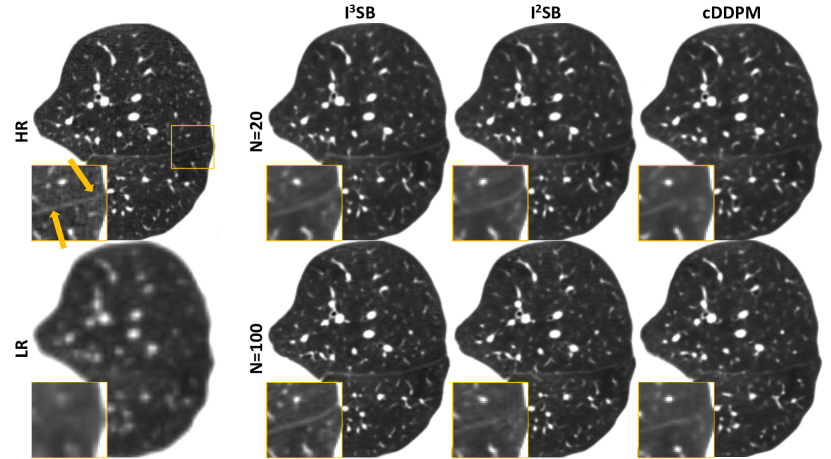
Figure 2: Results from the 4$\times$ chest CT super-resolution task. The restored anatomical features within the yellow box are zoomed in for enhanced visual clarity. The display window for the entire images is set to [-1000, -250] HU, and for the zoomed regions is set to [-1000, -550] HU.

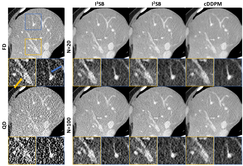
Figure 3: Results from the quarter-dose abdominal CT denoising task. The restored anatomical features within the yellow and blue boxes are zoomed in for enhanced visual clarity. The display window for the entire images is set to [-160, 240] HU, and for the zoomed regions is set to [50, 230] HU.

Table 1: Quantitative results of tested methods for the CT super resolution task. For 1000 steps cDDPM, the normalized Haralick feature distance is 0.507 and SSIM is 0.9323.

	Haralick (LR: 2.773)			SSIM (LR: 0.8757)
N	20	50	100	20	50	100
cDDPM	1.881	1.530	1.250	0.9492	0.9470	0.9443
I2SB	1.679	1.218	0.908	0.9482	0.9442	0.9405
I3SB	1.596	1.103	0.780	0.9476	0.9429	0.9384

Table 2: Quantitative results of tested methods for the CT denoising task. For 1000 steps cDDPM, the normalized Haralick feature distance is 0.391 and SSIM is 0.9429.

	Haralick (QD: 1.863)			SSIM (QD: 0.8731)
N	20	50	100	20	50	100
cDDPM	1.183	1.002	0.835	0.9539	0.9558	0.9541
I2SB	0.953	0.736	0.594	0.9581	0.9544	0.9510
I3SB	0.924	0.693	0.540	0.9577	0.9535	0.9495

3 Results

We conducted a comparative analysis between our proposed I³SB, I²SB and cDDPM. Apart from selecting $\beta_{t}$ according to the sigmoid schedule[9] in cDDPM, we maintained consistent network architecture and all training settings across all methods to ensure a fair comparison. Representative results are visualized in Fig. 2 and Fig. 3. A region containing a pulmonary fissure in the chest CT images and two regions containing hepatic veins in the abdominal CT images are zoomed in for enhanced visual clarity. I³SB and I²SB have better texture recovery and less oversmoothing at both 20 and 100 steps for both tasks compared to cDDPM. Compared to I²SB, I³SB managed to recover the entire fissure with $N=100$, where I²SB showed broken ends using the same time steps at the location indicated by the yellow arrow in Fig. 2. I³SB also has better recovery of the subtle vessel as pointed by the blue arrow as demonstrated in the $N=100$ results in Fig. 3.

For quantitative assessment of the texture restoration ability of these models, we calculated normalized Haralick feature distances [7, 15] within the external bounding box of the lungs for the chest CT dataset (window [-1000, 200] HU) and within the external bounding box of the liver for the abdominal CT dataset (window [-160, 240] HU). Additionally, to evaluate the models’ fidelity to the ground truth, structural similarity index measures (SSIMs) were computed within the external bounding box encompassing the entire chest or abdomen (window [-1000, 2000] HU). The quantitative results for the super resolution task are detailed in Table 1, and for the denoising task are detailed in Table 2.

Notably, the same tendency can be observed in both the CT super-resolution task and the CT denoising task. As $N$ increases, the normalized Haralick feature distances of both I²SB and I³SB become better, while the SSIMs worsen. This occurs because with an increased number of generative steps, these models tend to generate more details at the expense of some distortion from ground truth[4]. With the same number of generative steps, the SSIMs of cDDPM are negligibly better than those of I²SB and I³SB, with a difference of less than 0.5% for most of the cases, indicating that the three methods have similar level of fidelity of the restored images. However, cDDPM’s normalized Haralick feature distances are much worse, with relative increases from 15% to 60%. This is inline with our observation from Figs. 2 and 3 that cDDPM produces oversmoothing results compared to the other two. Compared with I²SB, our proposed I³SB achieves 5% to 10% better normalized Haralick feature distances with negligible worse SSIMs (<0.5%), suggesting that I³SB can generate more detailed images while maintaining consistency with ground truth established by I²SB.

4 Conclusion and Discussion

In conclusion, we proposed I³SB, a novel model that extends the generative process of I²SB to a non-Markovian process that incorporates corrupted images in each generative step. This innovation enables the generation of more detailed images without increasing distortion. Compared to I²SB and cDDPM, I³SB achieved similar fidelity but improved texture recovery in both CT super-resolution and denoising tasks. Furthermore, the hyperparameter $g_{n}$ introduces flexibility into the inference of I²SB with almost no additional cost.

I³SB shows promise for further refinement in the design of $g_{n}$, which regulates stochastic uncertainty and the weighting of $\hat{X}_{0}$, $X_{n+1}$, and $X_{N}$ during image generation. While $g_{n}$ is currently a simple step function of $n$, our future work aims to develop $g_{n}$ as a function of $\hat{X}_{0}$, $X_{n+1}$, $X_{N}$, and $n$. Additionally, we intend to integrate reinforcement learning into I³SB to enable $g_{n}$ to adapt autonomously, potentially offering significant enhancements to our proposed model.

References

- [1] AAPM: Low dose ct grand challenge. [Online] (2017), available: http://www.aapm.org/GrandChallenge/LowDoseCT/
- [2] Chen, T., Liu, G.H., Theodorou, E.A.: Likelihood training of schrödinger bridge using forward-backward sdes theory. arXiv preprint arXiv:2110.11291 (2021)
- [3] Chen, Y., Georgiou, T.T., Pavon, M.: Stochastic control liaisons: Richard sinkhorn meets gaspard monge on a schrodinger bridge. Siam Review 63(2), 249–313 (2021)
- [4] Chung, H., Kim, J., Ye, J.C.: Direct diffusion bridge using data consistency for inverse problems. Advances in Neural Information Processing Systems 36 (2024)
- [5] De Bortoli, V., Thornton, J., Heng, J., Doucet, A.: Diffusion schrödinger bridge with applications to score-based generative modeling. Advances in Neural Information Processing Systems 34, 17695–17709 (2021)
- [6] Delbracio, M., Milanfar, P.: Inversion by direct iteration: An alternative to denoising diffusion for image restoration. arXiv preprint arXiv:2303.11435 (2023)
- [7] Haralick, R.M., Shanmugam, K., Dinstein, I.H.: Textural features for image classification. IEEE Transactions on systems, man, and cybernetics 3(6), 610–621 (1973)
- [8] Ho, J., Jain, A., Abbeel, P.: Denoising diffusion probabilistic models. Advances in neural information processing systems 33, 6840–6851 (2020)
- [9] Jabri, A., Fleet, D., Chen, T.: Scalable adaptive computation for iterative generation. arXiv preprint arXiv:2212.11972 (2022)
- [10] Li, H., Yang, Y., Chang, M., Chen, S., Feng, H., Xu, Z., Li, Q., Chen, Y.: Srdiff: Single image super-resolution with diffusion probabilistic models. Neurocomputing 479, 47–59 (2022)
- [11] Liu, G.H., Vahdat, A., Huang, D.A., Theodorou, E.A., Nie, W., Anandkumar, A.: I2sb: Image-to-image schrödinger bridge. arXiv preprint arXiv:2302.05872 (2023)
- [12] Saharia, C., Ho, J., Chan, W., Salimans, T., Fleet, D.J., Norouzi, M.: Image super-resolution via iterative refinement. IEEE Transactions on Pattern Analysis and Machine Intelligence 45(4), 4713–4726 (2022)
- [13] Song, J., Meng, C., Ermon, S.: Denoising diffusion implicit models. arXiv preprint arXiv:2010.02502 (2020)
- [14] Wang, X., Xie, L., Dong, C., Shan, Y.: Real-esrgan: Training real-world blind super-resolution with pure synthetic data. In: Proceedings of the IEEE/CVF international conference on computer vision. pp. 1905–1914 (2021)
- [15] Wu, D., Kim, K., El Fakhri, G., Li, Q.: Iterative low-dose ct reconstruction with priors trained by artificial neural network. IEEE transactions on medical imaging 36(12), 2479–2486 (2017)
- [16] Yu, P., Zhang, H., Kang, H., Tang, W., Arnold, C.W., Zhang, R.: Rplhr-ct dataset and transformer baseline for volumetric super-resolution from ct scans. In: International Conference on Medical Image Computing and Computer-Assisted Intervention. pp. 344–353. Springer (2022)