Decoupled Data Consistency with Diffusion Purification for Image Restoration

Abstract

Diffusion models have recently gained traction as a powerful class of deep generative priors, excelling in a wide range of image restoration tasks due to their exceptional ability to model data distributions. To solve image restoration problems, many existing techniques achieve data consistency by incorporating additional likelihood gradient steps into the reverse sampling process of diffusion models. However, the additional gradient steps pose a challenge for real-world practical applications as they incur a large computational overhead, thereby increasing inference time. They also present additional difficulties when using accelerated diffusion model samplers, as the number of data consistency steps is limited by the number of reverse sampling steps. In this work, we propose a novel diffusion-based image restoration solver that addresses these issues by decoupling the reverse process from the data consistency steps. Our method involves alternating between a reconstruction phase to maintain data consistency and a refinement phase that enforces the prior via diffusion purification. Our approach demonstrates versatility, making it highly adaptable for efficient problem-solving in latent space. Additionally, it reduces the necessity for numerous sampling steps through the integration of consistency models. The efficacy of our approach is validated through comprehensive experiments across various image restoration tasks, including image denoising, deblurring, inpainting, and super-resolution.

Keywords: diffusion model, inverse problem, image restoration, consistency model, latent diffusion, diffusion purification

1 Introduction

Image restoration problems naturally arise in many computer vision and biomedical imaging applications, examples of which include image denoising, deblurring, inpainting, and super-resolution [1, 2, 3]. The objective of solving an image restoration problem, also known as an inverse problem, is to estimate an unknown signal $\bm{x}_{\star}\in\mathbb{R}^{n}$ from its corrupted or subsampled measurements $\bm{y}\in\mathbb{R}^{m}$ of the following form:

$$\bm{y}\;=\;\mathcal{A}(\bm{x}_{\star})+\bm{n},$$ (1)

where $\mathcal{A}:\mathbb{R}^{n}\rightarrow\mathbb{R}^{m}$ is a (nonlinear) forward operator, and $\bm{n}\in\mathbb{R}^{m}$ is additive noise.

In practice, the number of observed measurements is often significantly smaller than the input dimension (i.e., $m\ll n$), making the problem highly ill-posed and resulting in infinitely many solutions that satisfy Equation (1). To deal with this challenge, a common approach is to regularize the solution via enforcing image priors. In the field of image restoration, traditional priors such as sparsity have been thoroughly explored [2]. However, recent advancements have shifted focus towards employing deep generative models as learned priors for image restoration. This shift largely came to fruition by the work of Bora et al. [4], who demonstrated that deep generative models could achieve superior image reconstruction quality with fewer number of measurements compared to traditional sparsity-based methods [4, 5, 6]. Following this groundbreaking study, there has been a surge of interest in investigating and exploring various deep generative models for solving image restoration tasks, including deep image priors [7], compressed sensing with generative models (CSGM) [4], and their subsequent developments [1].

More recently, there has been a lot of attention in using diffusion models as image priors, as diffusion models have shown to achieve superior image sampling quality compared to existing generative methods [8, 9, 10, 11]. However, unlike with other types of generative models, adapting diffusion models as image priors to solve inverse problems is not straightforward. This is because the sampling (or generative) process for diffusion models is generally formulated for sampling from an unconditional distribution $p(\bm{x})$, where $p(\bm{x})$ denotes the data distribution. In contrast, solving inverse problems involves sampling from the conditional distribution $p(\bm{x}|\bm{y})$ to ensure data consistency. To sample from this conditional distribution, we need access to the likelihood gradients $\nabla_{\bm{x}_{t}}\log p(\bm{y}|\bm{x}_{t})$, which are intractable. Many earlier existing works tackle this issue with projection-type methods that project the unconditional sample $\bm{x}_{t}$ at each iteration $t$ onto the measurement subspace during the sampling process [9, 12, 13, 14, 15]. However, since the projection step is vulnerable to measurement noise and can only be applied to linear inverse problems, more recent works deal with this issue by directly approximating the conditional score function $\nabla_{\bm{x}_{t}}\log p(\bm{y}|\bm{x}_{t})$ throughout the sampling process under certain assumptions [16, 17, 18].

However, most (if not all) of these existing techniques encounter inherent challenges due to the coupled nature of data consistency and the sampling process. That is, the data consistency step usually takes place within the reverse sampling process of diffusion models, resulting in several fundamental limitations. Firstly, notice that the quality of the reconstructed image is highly dependent on the total number of data consistency steps that we perform. Since data consistency occurs within the reverse sampling process, the total number of data consistency steps can only be at most the total number of sampling steps. This severely limits the usage of accelerated diffusion model samplers, such as denoising diffusion implicit models (DDIMs) [11] and consistency models [19], which perform one-step sampling. Secondly, this coupling also makes it difficult to generalize existing methods to latent (or stable) diffusion, as recent works [20, 21] have demonstrated that simply adding the likelihood gradient for data consistency in the presence of latent diffusion models is insufficient for maintaining data consistency. This restriction hinders usability in large-scale image restoration tasks, where fast and accurate inference is essential.

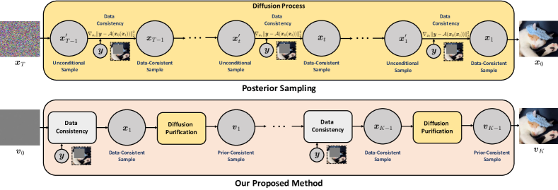
Figure 1: Illustration of the difference between our proposed method and existing posterior sampling techniques for image restoration. Our method decouples the data consistency step from the diffusion process, whereas existing methods incorporate data consistency into the reverse sampling process of diffusion models by taking an additional gradient step towards the measurement space.

Our Contributions.

In this study, we address these challenges by decoupling the data consistency and reverse sampling processes. Our algorithm involves a two-stage process that alternates between (i) generating initial estimations that are consistent with the measurements by minimizing the data fidelity objective and (ii) refining the initial estimations by incorporating the image prior via diffusion purification [22]. This effectively decouples the two processes, which consequently has two advantages over the state-of-the-art diffusion model methods for image restoration:

• Framework Versatility. Compared to existing methods, our framework can easily incorporate any diffusion model in a plug-and-play fashion. We demonstrate this flexibility by presenting experimental results that effectively leverage both latent diffusion and consistency models for image restoration.

• Improved Efficiency. We demonstrate that by decoupling these processes, we can significantly reduce inference time by more than $5\times$, all while achieving state-of-the-art performance. This contribution is particularly notable because we can incorporate accelerated samplers without approximating the conditional score functions, as was done in previous works.

We conduct thorough experiments to validate our method and its advantages across a wide range of image restoration problems, including super-resolution, inpainting, and image deblurring.

Throughout these tasks, we demonstrate that our method can outperform existing methods across several quantitative metrics and perform extensive ablation studies to highlight our approach.

Notation and Organization.

The remainder of this paper is organized as follows. In Section 2, we briefly discuss the essential preliminaries. Subsequently, we introduce our proposed framework in Section 3. Moreover, we further introduce acceleration techniques of our approach in Section 4. In Section 5, we validate the effectiveness of our algorithm with experiments on various image restoration problems. In Sections 6 and 7, we discuss the relationship of our work with prior art, limitation and future directions. All extra technical details are postponed to the appendices.

We denote scalar (function) as regular lower-case letters (e.g. $s_{t},f(t)$), vectors (function) with bold lower-case letters (e.g. $\bm{x},\bm{s}(\bm{x}_{t},t)$). We use $[N]$ to denote the set $\{1,2,\ldots,N\}$, $\mathbb{P}(\cdot)$ to denote the probability, $\mathbb{E}\left[\cdot\right]$ to denote expectation, $||\cdot||_{2}$ to denote L2 norm, $\mathcal{N}(\cdot)$ to denote gaussian distribution. We use $\bm{x}_{t}$ to denote a sample $\bm{x}$ at time step $t$. We use $\bm{x}_{0}$ to denote a clean sample, and use $\bm{s}_{\bm{\theta}}$ and $\bm{s}_{\bm{\phi}}$ for the estimated score functions in the pixel and latent spaces, respectively (discussed in detail later).

2 Preliminaries

In this section, we first briefly review the basic fundamentals of diffusion models [23, 8, 9, 10, 24, 25] and then discuss how to adapt them for solving image restoration problems. Subsequently, we present the main ideas behind diffusion purification, which serve as the backbone of our proposed method.

2.1 Unconditional Diffusion Models

Diffusion models [23, 8, 9, 10] generate an image with two processes, generally referred to as forward and reverse processes. The forward process is to diffuse the data distribution $p_{0}(\bm{x})$ to a standard Gaussian $p_{T}(\bm{x})=\mathcal{N}(\bm{0},\bm{I})$ by gradually injecting noise. In the variance-preserving (VP) setting [26], the forward process can be written as a stochastic differential equation (SDE) of the form

$$d\bm{x}_{t}\;=\;-\frac{\beta_{t}}{2}\bm{x}_{t}dt+\sqrt{\beta_{t}}d\bm{w},$$ (2)

where $\beta_{t}>0$ controls the speed of diffusion and $\bm{w}$ follows the standard Wiener process. To sample an image, we can employ the reverse SDE, which takes the form

$$d\bm{x}_{t}\;=\; \left[-\frac{\beta_{t}}{2}{\bm{x}_{t}}-\beta_{t}\nabla_{\bm{x}_{t}}\log p_{t}(\bm{x}_{t})\right]dt+\sqrt{\beta_{t}}d\bar{\bm{w}},$$ (3)

where $p_{t}(\bm{x}_{t})$ is the distribution of $\bm{x}_{t}$ at the time $t$, $\nabla_{\bm{x}_{t}}\log p_{t}(\bm{x}_{t})$ is the (Stein) score function, and $\bar{\bm{w}}$ follows the reverse Wiener process [27]. In practice, we estimate the score function using a deep neural network $\bm{s}_{\bm{\theta}}:\mathbb{R}^{n}\times[0,1]\rightarrow\mathbb{R}^{n}$ parameterized by $\bm{\theta}$, which is trained using the denoising score matching objective [28]:

$$\underset{\bm{\theta}}{\min}\,\mathbb{E}_{t,\bm{x}_{0},\bm{x}_{t}|\bm{x}_{0}}\left[\left\|\bm{s}_{\bm{\theta}}(\bm{x}_{t},t)-\nabla_{\bm{x}_{t}}\log p_{0t}(\bm{x}_{t}|\bm{x}_{0})\right\|_{2}\right],$$

where $t\sim\mathcal{U}(0,1)$, $\bm{x}_{0}\sim p_{0}(\bm{x})$, and $\bm{x}_{t}|\bm{x}_{0}\sim p_{0t}(\bm{x}_{t}|\bm{x}_{0})$. In practice, both the forward and reverse SDE can be discretized, with

$$\bm{x}_{t} =\sqrt{1-\beta_{t}}\bm{x}_{t-1}+\sqrt{\beta_{t}}\bm{\epsilon}_{t-1},$$

$$\bm{x}_{t-1} =\frac{1}{\sqrt{1-\beta_{t}}}\left(\bm{x}_{t}+\beta_{t}\nabla_{\bm{x}_{t}}\log p_{t}(\bm{x}_{t})\right)+\sqrt{\beta_{t}}\bm{\epsilon}_{t},$$

where $\bm{\epsilon}_{t}\sim\mathcal{N}(0,\bm{I})$.

2.2 Diffusion Models for Image Restoration Problems

To solve image restoration problems with diffusion models, one of the most commonly used techniques is to modify the unconditional reverse sampling process in Equation 3 by replacing the unconditional score with a conditional score function $\nabla_{\bm{x}_{t}}\log p_{t}(\bm{x}_{t}|\bm{y})$ based on $\bm{y}$. As such, the conditional reverse SDE has the following form

$$d\bm{x}_{t}\;=\;\left[-\frac{\beta_{t}}{2}{\bm{x}_{t}}-\beta_{t}\{\nabla_{\bm{x}_{t}}\log p_{t}(\bm{x}_{t}|\bm{y})\}\right]dt+\sqrt{\beta_{t}}d\bar{\bm{w}}.$$

Then, by Bayes rule, we can decompose the conditional score function $\nabla_{\bm{x}_{t}}\log p_{t}(\bm{x}_{t}|\bm{y})$ into

$$\nabla_{\bm{x}_{t}}\log p_{t}(\bm{x}_{t}|\bm{y})=\nabla_{\bm{x}_{t}}\log p_{t}(\bm{x}_{t})+\nabla_{\bm{x}_{t}}\log p_{t}(\bm{y}|\bm{x}_{t}).$$

While the unconditional prior score $\nabla_{\bm{x}_{t}}\log p_{t}(\bm{x}_{t})$ can be obtained from a pre-trained diffusion model, the likelihood gradient $\nabla_{\bm{x}_{t}}\log p_{t}(\bm{y}|\bm{x}_{t})$ is usually intractable.

To tackle this issue, recent works [16, 17, 18] resort to approximating the likelihood term with tractable surrogates, built upon the idea of diffusion posterior sampling (DPS) [16]. DPS approximates the likelihood gradient with

$$\nabla_{\bm{x}_{t}}\log p_{t}(\bm{y}|\bm{x}_{t})\approx\eta\nabla_{\bm{x}_{t}}\|\mathcal{A}(\hat{\bm{x}}_{0}(\bm{x}_{t}))-\bm{y}\|_{2}^{2},$$ (4)

where $\eta>0$ can be viewed as a step size for controlling the data consistency strength and $\hat{\bm{x}}_{0}(\bm{x}_{t}):=\mathbb{E}[\bm{x}_{0}|\bm{x}_{t}]$ is the posterior mean, which can be estimated through Tweedie’s formula [29, 30]:

$$\hat{\bm{x}}_{0}(\bm{x}_{t}) =\frac{1}{\bar{\alpha}_{t}}(\bm{x}_{t}-\sqrt{1-\bar{\alpha}_{t}}\nabla_{\bm{x}_{t}}\log p(\bm{x}_{t}))$$

$$\approx\frac{1}{\bar{\alpha}_{t}}(\bm{x}_{t}-\sqrt{1-\bar{\alpha}_{t}}\bm{s}_{\bm{\theta}}(\bm{x}_{t},t)).$$

However, despite being one of the most recognized algorithms, DPS suffers from several limitations, as previously briefly illustrated. Firstly, the inference time of the reverse sampling process is significantly increased, as the likelihood estimation needs to backpropagate over the entire score function $\bm{s}_{\bm{\theta}}(\bm{x}_{t},t)$ for each iteration $t$ of the sampling process. Since the score function is generally parameterized as a large deep network, this process can be computationally challenging, especially for tasks involving high-dimensional images. Secondly, as the data consistency steps take place within the reverse sampling process, the number of gradient steps for data consistency is limited by the reverse sampling steps, which could lead to insufficient data consistency when using accelerated samplers such as consistency models [19]. Furthermore, the performance of DPS is sensitive to the step size $\eta$ due to the coupled data consistency and reverse sampling. When $\eta$ is small, the reconstructions will not be consistent with the measurements $\bm{y}$. On the other hand, a large $\eta$ may push $\bm{x}_{t}$ away from the noisy data manifold on which the diffusion model is trained, resulting in serious artifacts. Lastly, naively adapting DPS to latent diffusion models often fails due to the nonlinearity of the decoder. Since most diffusion-based image restoration solvers are built upon the idea of DPS, they all suffer from these fundamental issues, motivating the need to decouple the data consistency and reverse sampling processses.

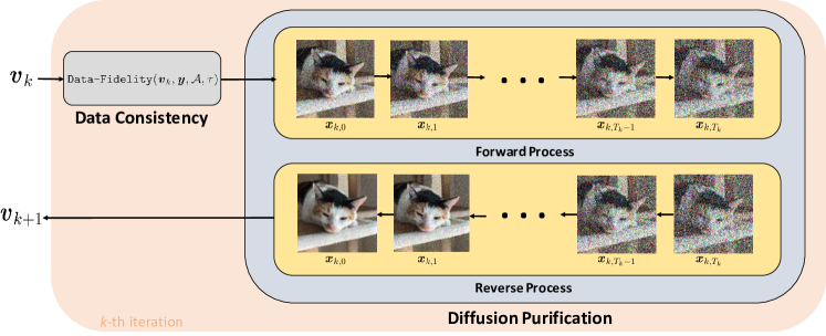
Figure 2: An illustration of our overall framework. Our algorithm involves a total of $K$ iterations which alternate between (i) generating an initial reconstruction by solely optimizing the data fidelity objective and (ii) refining the image via diffusion purification.

2.3 Diffusion Purification

Recently, diffusion purification has shown to be an effective approach for removing adversarial perturbations [22, 31] and for image editing [32]. Specifically, for a given noisy or perturbed image $\bm{x}_{\textrm{adv}}$, this process involves first running the diffusion forward process as described in Equation (2) starting from $\bm{x}_{\textrm{adv}}$ to some intermediate timestep $T$. In the discrete case, $\bm{x}_{T}$ takes the form

$$\bm{x}_{T}=\sqrt{\bar{\alpha}_{T}}\bm{x}_{\textrm{adv}}+\sqrt{(1-\bar{\alpha}_{T})}\bm{\epsilon}\>,$$ (5)

where $\bar{\alpha}_{T}=\prod_{t=1}^{T}(1-\beta_{t})$. Starting with $\bm{x}_{T}$, we implement the reverse diffusion process with Equation (3) to produce a “purified” image $\bm{x}_{\textrm{purified}}$, effectively eliminating the adversarial perturbations. The rationale behind this is that by carefully selecting $T$, the adversarial noise within $\bm{x}_{\textrm{adv}}$ becomes overwhelmed by the noise introduced during the forward phase, yet the core semantic information is preserved. Consequently, executing the reverse diffusion process leads to a “clean” image reconstruction. In our work, we use diffusion purification as the backbone of our approach, yet with a distinct objective diverging from existing methods that use diffusion purification to enhance the robustness of DNN-based classifiers [22] or remove artifacts in medical imaging [33, 31].

3 Proposed Methods

In this section, we first introduce our method for image restoration based upon variable splitting (Section 3.1). Then, in Section 3.2, we discuss enforcing data consistency, followed by our proposed method to use diffusion models as an image prior via diffusion purification (Section 3.3). The entire procedure of the proposed method is outlined in Algorithm 1.

3.1 Methods with Variable Splitting

Our proposed algorithm is inspired by the classical variable splitting technique [34, 35, 36, 37] in optimization. Specifically, consider the following regularized optimization formulation for the image restoration problem in Equation 1,

$$\min_{\bm{x}}\frac{1}{2}\left\|\mathcal{A}(\bm{x})-\bm{y}\right\|_{2}^{2}+\lambda\mathcal{R}(\bm{x}),$$

where $\mathcal{R}(\cdot)$ is the regularization for image prior, and $\lambda>0$ controls the penalty strength. The idea of variable splitting is to introduce an auxiliary variable $\bm{v}=\bm{x}$ to pose an equivalent problem

$$\min_{\bm{x},\bm{v}}\frac{1}{2}\left\|\mathcal{A}(\bm{x})-\bm{y}\right\|_{2}^{2}+\lambda\mathcal{R}(\bm{v}),\;\mathrm{s.t.}\;\bm{x}=\bm{v}.$$ (6)

This constrained optimization problem can be relaxed into an unconstrained problem by the half quadratic splitting technique (HQS) [38, 37], which we can reformulate as

$$\min_{\bm{x},\bm{v}}\underbrace{\frac{1}{2}\left\|\mathcal{A}(\bm{x})-\bm{y}\right\|_{2}^{2}+\frac{\mu}{2}\|\bm{x}-\bm{v}\|_{2}^{2}+\lambda\mathcal{R}(\bm{v})\>,}_{=:\mathcal{L}(\bm{x},\bm{v})}$$ (7)

for some properly chosen $\mu>0$. Then, to solve Equation 7, we can use an iterative method such that for every iteration $k$, we can leverage the extra variable $\bm{v}$ to split the optimization into two sub-problems of the form

$$\bm{x}_{k}=\operatorname*{\text{arg~{}min}}_{\bm{x}}\;\mathcal{L}(\bm{x},\bm{v}_{k-1}),$$ (8)

$$\bm{v}_{k}=\operatorname*{\text{arg~{}min}}_{\bm{v}}\;\mathcal{L}(\bm{x}_{k},\bm{v}),$$ (9)

that decouples the data consistency term $\left\|\mathcal{A}(\bm{x})-\bm{y}\right\|_{2}^{2}$ from the regularization term $\mathcal{R}(\bm{v})$. Then, instead of having an explicit regularizer $\mathcal{R(\cdot)}$ (e.g., $\ell_{1}$-norm to induce sparsity), we can use implicit regularizers. More specifically, we can constrain the output space as the range of the diffusion model via diffusion purification that acts as a form of regularization or prior. To enforce this implicit regularizer, our method involves alternating between the two following steps:

1. Data Consistency. Generate measurement-consistent reconstructions, which may have various artifacts, by solving the data consistency optimization problem Equation 8.

2. Regularization via Diffusion Purification. Refine the obtained reconstruction from the previous step with a pre-trained diffusion model via diffusion purification.

In the following subsections, we dive into the technical details of each step and present an illustration of our method in Figure 2. We also conduct an ablation study in Section 5.3, demonstrating that alternating between these two steps can decrease the distance between the reconstructed and the target image.

Algorithm 1 Image Restoration with Decoupled Data Consistency and Diffusion Model Prior

measurements $\bm{y}$, forward operator $\mathcal{A}(\cdot)$, pretrained model $\bm{s}_{\bm{\theta}}$, total number of iterations $K$, decaying time schedule $\{T_{k}\}_{k\in[K]}$ for diffusion purification, iteration number $\tau$, and $\bm{v}_{0}=\bm{0}\in\mathbb{R}^{n}$

for $k=1,\dots,K$ do

     $\bm{x}_{k}=\texttt{Data-Fidelity}(\bm{v}_{k-1},\bm{y},\mathcal{A},\tau)$ $\triangleright$ solve via gradient based methods

     $\bm{v}_{k}=\texttt{DPUR}(\bm{x}_{k},\bm{s}_{\bm{\theta}},T_{k})$ $\triangleright$ Diffusion Purification

end for

Return $\bm{v}_{k}$

3.2 Enforcing Data Consistency

Recall that the sub-problem in Equation (8) for maintaining data consistency can be written as

$$\bm{x}_{k}=\operatorname*{\text{arg~{}min}}_{\bm{x}}\;\frac{1}{2}\|\mathcal{A}(\bm{x})-\bm{y}\|_{2}^{2}+\mu\|\bm{x}-\bm{v}_{k-1}\|_{2}^{2}\>.$$

The difficulty behind directly solving the above problem lies in selecting the proper hyperparameter $\mu$, as it may need to be frequently tuned. To tackle this issue, we instead seek an approximate solution $\bm{x}_{k}$ that minimizes solely the data fidelity term $\frac{1}{2}\|\mathcal{A}(\bm{x})-\bm{y}\|_{2}^{2}$ but starting the optimization with $\bm{v}_{k-1}$ as the initial point and run a limited number of $\tau$ gradient steps, resulting in a measurement-consistent reconstruction $\bm{x}_{k}$. The rationale behind this is two-fold: (i) by taking $\bm{v}_{k-1}$ as the initial point, we can obtain an output $\bm{x}_{k}$ that is sufficiently close to $\bm{v}_{k-1}$ without having to tune $\mu$, and (ii) taking a limited number of gradient steps $\tau$ reduces the computational burden. Overall, for simplicity, we denote this step as

$$\bm{x}_{k}=\texttt{Data-Fidelity}(\bm{v}_{k-1},\bm{y},\mathcal{A},\tau).$$ (10)

Lastly, we want to highlight that our technique for enforcing data consistency is significantly more efficient than existing methods, as our method does not require back propagation over the entire score function (i.e., the neural network) and hence is (very) computationally efficient. Furthermore, to enforce data consistency, we can use any momentum-based gradient descent optimizer (e.g., SGD, ADAM) for Equation 10. Throughout the experiment we fix the number of gradient steps $\tau$ for each round of the data fidelity optimization. When the measurements are corrupted by noise, one can further reduce the number of iteration to prevent overfitting. We discuss our choice of optimizers in Appendix A.

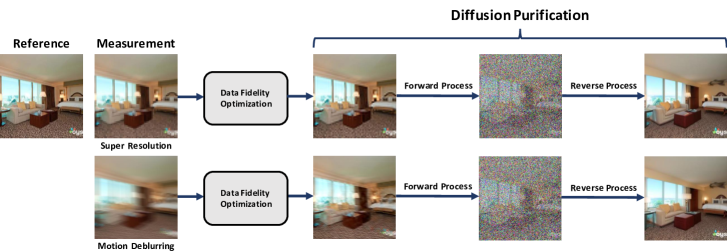
Figure 3: Demonstrating the regularization effects of diffusion purification. The estimates from the data fidelity step contain artifacts, making the overall reconstruction inaccurate, whereas regularization via diffusion purification can remove such artifacts.

3.3 Implicit Regularization by Diffusion Purification

Due to the underdetermined nature of the problem (1), the initial reconstruction $\bm{x}_{k}$ obtained from Equation 10 will suffer from task specific artifacts, as shown in Figure 3 (the third column). The next step is to refine $\bm{x}_{k}$ via enforcing the image prior learned by the diffusion model. To do so, we propose to utilize diffusion purification described in Section 2.3 as an implicit regularizer for effectively removing the artifacts in $\bm{x}_{k}$ as shown in Figure 3. More specifically, let $T_{k}$ denote the diffusion purification strength at iteration $k$. Following the diffusion purification step in Equation (5), we first define $\bm{x}_{k,0}:=\bm{x}_{k}$ and submerge this sample with noise up to time $T_{k}$:

$$\bm{x}_{k,T_{k}}=\sqrt{\bar{\alpha}_{T_{k}}}\bm{x}_{k,0}+\sqrt{1-\bar{\alpha}_{T_{k}}}\bm{\epsilon}.$$ (11)

Then, we run unconditional reverse sampling via the reverse SDE in Equation 3 starting from $\bm{x}_{k,T_{k}}$ to obtain the output $\bm{v}_{k}$. Concretely, the discretized version of the reverse SDE can be described as

$$\bm{x}_{k,t-1}= \frac{1}{\sqrt{1-\beta_{t}}}\left(\bm{x}_{k,t}+\beta_{t}\bm{s}_{\bm{\theta}}(\bm{x}_{k,t},t)\right)+\sqrt{\beta_{t}}\bm{\epsilon}_{t},$$ (12)

for $t=T_{k},T_{k}-1,\ldots,1$. Here, recall that $\bm{s}_{\bm{\theta}}(\bm{x},t)$ denotes the score function which can be estimated by a pre-trained unconditional diffusion model. For simplicity, we denote this overall regularization step by

$$\bm{v}_{k}=\texttt{DPUR}(\bm{x}_{k},\bm{s}_{\bm{\theta}},T_{k}).$$ (13)

For the choice of $T_{k}$, we propose to use a linear decaying schedule for robust performance, which is capable of addressing the “hallucination” issue brought by the stochasticity of the diffusion purification process. In the early iterations of our method, when $T_{k}$ is relatively large, the resulting $\bm{v}_{k}$, though may be inconsistent with the measurements, will be free from artifacts and can serve as good starting point for the subsequent iteration of data consistency optimization. As $T_{k}$ keeps decreasing, the algorithm will converge to an equilibrium point which is both consistent with the measurements and free from the artifacts. More technical details are deferred to Appendix A, and we study the convergence in Section 5.3.

4 Adaptability to Accelerated Samplers & Latent Diffusion

One of the main drawbacks of diffusion models is the increased inference time of the iterative sampling process compared to traditional methods such as variational autoencoders (VAEs) [39] and generative adversarial networks (GANs) [40]. In the literature, many advancements have been made to address this issue, which involve either decreasing the number of iterations via accelerated sampling techniques such as DDIMs [11] or carrying out the sampling process in a lower-dimensional, latent space [24, 25]. In the following sections, we briefly introduce these techniques and demonstrate how they can be used to decrease the inference time of diffusion purification, thereby accelerating our algorithm.

4.1 Faster Diffusion Purification

To improve sampling efficiency, we can adopt the use of accelerated samplers to decrease the sampling time of the reverse process of diffusion purification. For example, we can use the accelerated sampler DDIM, which constructs a non-Markovian chain of the reverse process. By doing so, we can perform each round of diffusion purification with as few as $20$ unconditional reverse sampling steps (i.e., $20$ number of function evaluations (NFEs)), with minimal performance degradation.

Here, we would like to remark that existing methods such as DPS do not have this advantage. DPS typically requires approximately $1000$ reverse sampling steps, as it requires more iterations to ensure “sufficient” data consistency steps.

In the following, we discuss the adaptability of our approach using one-step sampling approaches, including consistency models and approximations via Tweedie’s formula.

Consistency Models.

Recently, Song et al. [19] proposed a class of diffusion models termed consistency models (CMs), which can effectively generate high-quality samples in a single (or at least very few) time steps. CMs build on the fact that there exists a deterministic ODE for every corresponding SDE sampling trajectory of Equation 3 in the form of

$$d\bm{x}_{t}\;=\;\left[-\frac{\beta_{t}}{2}{\bm{x}_{t}}-\frac{\beta_{t}}{2}\nabla_{\bm{x}_{t}}\log p_{t}(\bm{x}_{t})\right]dt,$$ (14)

with which it shares the same probability densities $p_{t}(\bm{x}_{t})$ for all $t\in[0,1]$ [9]. This implies that for any image $\bm{x}_{0}$, there exists a unique ODE trajectory $\{\bm{x}_{t}\}_{t=0}^{1}$. By leveraging this property, CMs train a deep network $f_{\bm{\theta}}:\mathbb{R}^{d}\times[0,1]\rightarrow\mathbb{R}^{d}$ parameterized by $\bm{\theta}$ to map any point $\bm{x}_{t}$ to its corresponding $\bm{x}_{0}$ in a single step.

This approach can be seamlessly incorporated into our framework. Specifically, with a pre-trained consistency model $f_{\bm{\theta}}$, the diffusion purification step in Equation 13 in Algorithm 1 can be performed in a single step as

$$\bm{v}_{k}=\texttt{DPUR}(\bm{f}_{\bm{\theta}},\bm{x}_{k},T_{k}):=f_{\bm{\theta}}(\bm{x}_{k},T_{k}).$$ (15)

Approximation via Tweedie’s Formula.

Under a Gaussian assumption, Tweedie’s formula [29, 30] provides a way of computing the posterior mean by using

$$\mathbb{E}\left[\bm{x}_{0}\mid\bm{x}_{t}\right]=\frac{1}{\bar{\alpha}_{t}}(\bm{x}_{t}-\sqrt{1-\bar{\alpha}_{t}}\nabla_{\bm{x}_{t}}\log p(\bm{x}_{t})),$$

where $\bm{x}_{0}$ denotes a sample from the “clean” data distribution. Equipped with this formula, instead of running the reverse SDE in Equation 12 for diffusion purification, one can estimate the ground truth in a single step using this formula. Specifically, we can approximate $\bm{v}_{k}$ using

$$\bm{v}_{k} =\mathbb{E}\left[\bm{x}_{k,0}\mid\bm{x}_{k,T_{k}}\right]\approx\frac{1}{\sqrt{\bar{\alpha}_{T_{k}}}}(\bm{x}_{k,T_{k}}+\sqrt{1-\bar{\alpha}_{T_{k}}}\bm{s}_{\bm{\theta}}(\bm{x}_{k,T_{k}},T_{k}))\>,$$

where the approximation arises from the score function estimation and $\bm{x}_{k,T_{k}}$ is a sample at iteration $k$ diffused upto switching time $T_{k}$ via the forward process.

Compared to reverse SDE sampling, employing Tweedie’s formula will lead to a tradeoff between computation time and reconstruction quality. As evidenced by our experimental results in Section 5, using Tweedie’s formula for approximating the reverse SDE may result in blurry reconstructions with lower perceptual quality, a phenomenon partly attributed to the ”regression to the mean” effects [41].

Algorithm 2 LDM Version of Our Method

measurements $\bm{y}$, forward operator $\mathcal{A}(\cdot)$, pretrained LDM $\bm{s}_{\bm{\phi}}$, a pair of pretrained encoder $\mathcal{E}$ and decoder $\mathcal{D}$, total number of iterations $K$, decaying time schedule $\{T_{k}\}_{k\in[K]}$ for diffusion purification, iteration number $\tau$, and $\widehat{\bm{v}}_{0}\sim\mathcal{N}(\bm{0},\bm{I})$ if enforcing data consistency in the latent space or $\mathcal{D}(\widehat{\bm{v}}_{0})=\bm{0}$ if enforcing data consistency in the pixel space.

for $k=1,\dots,K$ do

     if Approach I: enforcing data consistency in the latent space  then

         $\bm{z}_{k}=\texttt{Data-Fidelity-LDM}(\widehat{\bm{v}}_{k-1},\bm{y},\mathcal{A},\mathcal{D},\tau)$ $\triangleright$ Enforcing data consistency in the latent space

         $\bm{z}_{k}\leftarrow\mathcal{E}(\mathcal{D}(\bm{z}_{k}))$$\triangleright$ Re-Encode

     else if Approach II: enforcing data consistency in the pixel space  then

         $\bm{x}_{k}=\texttt{Data-Fidelity}(\mathcal{D}(\widehat{\bm{v}}_{k-1}),\bm{y},\mathcal{A},\tau)$ $\triangleright$ Enforcing data consistency in the pixel space

         $\bm{z}_{k}=\mathcal{E}(\bm{x}_{k})$ $\triangleright$ Mapping to the latent space

     end if

     $\widehat{\bm{v}}_{k}=\texttt{DPUR}(\bm{z}_{k},\bm{s}_{\bm{\phi}},T_{k})$ $\triangleright$ Latent diffusion purification

     $\bm{x}_{k}=\mathcal{D}(\bm{v}_{k})$ $\triangleright$ Mapping to the pixel space

end for

Return $\mathcal{D}(\bm{v}_{k})$

Lastly, notice that this approximation may seem similar to CMs, as they both necessitate only a single NFE. However, CMs avoid some of the tradeoffs discussed previously, as CMs were designed specifically for single-step sampling. Nevertheless, we illustrate the effectiveness of our framework on both techniques, demonstrating that one can use any model that is more readily available.

4.2 Adaptation to Latent Diffusion

Latent diffusion models (LDMs) [24, 25] operate in a lower-dimensional latent space by training a pair of encoder and decoder [42] to address the slow inference time of diffusion models. Specifically, given an encoder $\mathcal{E}:\mathbb{R}^{d}\to\mathbb{R}^{r}$ and a decoder $\mathcal{D}:\mathbb{R}^{r}\to\mathbb{R}^{d}$ where $r\ll d$, LDMs reduce the computational complexity by mapping each $\bm{x}\in\mathbb{R}^{d}$ to $\bm{z}=\mathcal{E}(\bm{x})\in\mathbb{R}^{r}$ and performing the entire diffusion process in the latent space. Then, upon running the reverse steps within the latent space, one can pass the sampled latent code $\bm{z}_{0}$ through the decoder to obtain a synthesized image $\bm{x}_{0}=\mathcal{D}(\bm{z}_{0})$.

Unlike previous methods [20, 21], the flexibility of our framework allows us to (almost) seamlessly incorporate LDMs. Similar to Section 3.1, we alternate between enforcing data consistency and diffusion purification but both in the latent space:

$$\bm{z}_{k} =\operatorname*{\text{arg~{}min}}_{\bm{z}}\;\mathcal{L}_{\mathrm{LDM}}(\bm{z},\widehat{\bm{v}}_{k-1}),$$ (16)

$$\widehat{\bm{v}}_{k} =\texttt{DPUR}(\bm{z}_{k},\bm{s}_{\bm{\phi}},T_{k}),$$ (17)

where $\mathcal{L}_{\mathrm{LDM}}$ is a loss function tailored for the latent space (discussed later), $\bm{s}_{\bm{\phi}}$ is the score function in the latent space, and $\bm{z}=\mathcal{E}(\bm{x})$ and $\widehat{\bm{v}}=\mathcal{E}(\bm{v})$. Once our method converges to a specific stopping criteria, we map the converged solution back to the pixel space through the decoder $\mathcal{D}$. The overall method is presented in Algorithm 2. In the following subsections, we discuss two approaches for enforcing DC using LDMs.

Approach I: Enforcing DC in the Latent Space.

One way of enforcing data consistency (DC) is strictly in the latent space. Specfically, we can consider the modified problem

$$\bm{z}_{k} =\operatorname*{\text{arg~{}min}}_{\bm{z}}\frac{1}{2}\|\bm{y}-\mathcal{A}(\mathcal{D}(\bm{z}))\|_{2}^{2}+\frac{\mu}{2}\|\bm{z}-\widehat{\bm{v}}_{k-1}\|_{2}^{2},$$

where $\widehat{\bm{v}}_{k-1}$ is the outcome of the previous diffusion purification step in the latent space. We remark that this problem is similar to the CSGM problem considered in [4].

Then, similar to Section 3.2, we can approximately solve the above problem by taking a limited number of gradient based steps on $\frac{1}{2}\|\bm{y}-\mathcal{A}(\mathcal{D}(\bm{z}))\|_{2}^{2}$ w.r.t. $\bm{z}$ starting from $\widehat{\bm{v}}_{k-1}$:

$$\bm{z}_{k}=\texttt{Data-Fidelity-LDM}(\widehat{\bm{v}}_{k-1},\bm{y},\mathcal{A},\mathcal{D},\tau).$$ (18)

Before the diffusion purification step, we run an extra step on the solution obtained from Equation 18

$$\bm{z}_{k} \leftarrow\mathcal{E}(\mathcal{D}(\bm{z}_{k})),$$ (19)

which we label “Re-Encode”. The rationale behind this seemingly unnecessary step is that due to the nonlinearity of the encoder $\mathcal{E}$, there exist infinitely many solutions $\bm{z}$ for the optimization problem in Equation 18. However, since the LDMs are trained only on $\bm{z}=\mathcal{E}(x)$, we need to first map $\bm{z}_{k}$ back to the image space with $\bm{x}_{k}=\mathcal{D}(\bm{z}_{k})$ and then re-encode $x_{k}$ as $z_{k}=\mathcal{E}(\bm{x}_{k})$.

Approach II: Enforcing DC in the Pixel Space.

Alternatively, we can also directly enforce the data consistency in the pixel space. Specifically, given $\widehat{\bm{v}}_{k-1}$ as the outcome of the previous diffusion purification step in the latent space, we can run

$$\bm{x}_{k} =\operatorname*{\text{arg~{}min}}_{\bm{x}}\frac{1}{2}\|\bm{y}-\mathcal{A}(\bm{x})\|_{2}^{2}+\frac{\mu}{2}\|\bm{x}-\mathcal{D}(\widehat{\bm{v}}_{k-1})\|_{2}^{2}.$$

Again, we can approximately solve the above problem by taking a limited number of gradient based steps on $\frac{1}{2}||\bm{y}-\mathcal{A}(\bm{x})||_{2}^{2}$ w.r.t. $\bm{x}$ starting from $\mathcal{D}(\widehat{\bm{v}}_{k-1})$:

$$\bm{x}_{k} =\texttt{Data-Fidelity}(\mathcal{D}(\widehat{\bm{v}}_{k-1}),\bm{y},\mathcal{A},\tau),$$ (20)

which is the same as Equation 10 with $\bm{v}_{k-1}=\mathcal{D}(\widehat{\bm{v}}_{k-1})$. Followed by this, we run

$$\bm{z}_{k} =\mathcal{E}(\bm{x}_{k}),$$

to use the encoder $\mathcal{E}$ to map $\bm{x}_{k}$ into the latent space $\bm{z}_{k}$ for the subsequent diffusion purification step in Equation 17.

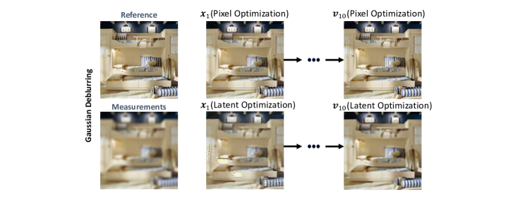
Figure 15: Comparison between Pixel Space Optimization and Latent Space Optimization for Gaussian Deblurring. Initial Reconstructions obtained via Pixel Space Optimization have much better quality compared to the ones obtained from Latent Space Optimization which in turn result in final reconstructions with higher quality.

Compared to Approach I, it is worth noting that Approach II is much more efficient. This is because here we do not require back propogation through the deep decoder $\mathcal{D}$ for computing the gradient. In practice, both methods are effective for a range of image restoration problems. However, we observe that Approach II tends to be more suitable for specific types of problems like motion deblurring and Gaussian deblurring. This is because it has a better capability to produce $\bm{x}_{k}$’s with superior quality compared to Approach I. See Figures 15 and 14 in Section A.1 for more detail.

5 Experiments

In this section, we demonstrate the effectiveness of our method under various settings. First, we introduce the basic experiment setup in Section 5.1. Second, we show our main experimental results in Section 5.2. Finally, we provide an ablation study in Section 5.3 in terms of noise robustness, computational efficiency, and convergence.

5.1 Experimental Setup

Types of Image Restoration Problems.

To demonstrate the effectiveness of our algorithm, we consider the following image restoration problems:

• Image inpainting with a $100\times 100$ size box mask.

• Image super-resolution with $4\times$ down sampling.

• Gaussian image deblurring with Gaussian kernel of size $61\times 61$ and standard deviation $\sigma=3.0$.

• Motion image deblurring with motion deblurring kernel size $61\times 61$ and intensity value $0.5$.

These image restoration problems are commonly explored in numerous relevant works [20, 21, 16, 13] and also arise in many practical applications.

Evaluation Datasets and Metrics.

To demonstrate the effectiveness of our method, we conducted experiments on the FFHQ [43] and LSUN-Bedroom [44] datasets, which have an image size of $256\times 256\times 3$. For CMs, we test our method only on the LSUN-Bedroom dataset as a proof-of-concept. Generally, images of bedrooms have more complicated structures than those in “face” image datasets, making them a good indicator of the efficacy of our algorithm.

To quantitatively evaluate the performance of the algorithms, we use standard metrics: (i) Peak Signal-to-Noise-Ratio (PSNR), (ii) Structural Similarity Index Measure (SSIM) [45] and (iii) Learned Perceptual Image Patch Similarity (LPIPS) [46]. These metrics are commonly used in existing works that evaluate image restoration techniques [21], and are shown to be an accurate indicator of reconstruction performance.

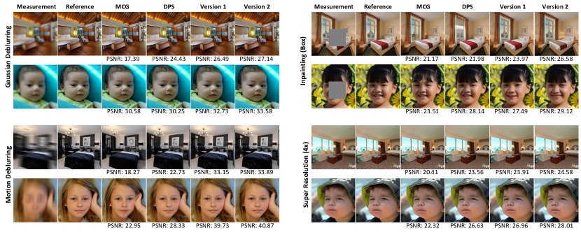
Figure 4: Pixel space diffusion models for solving various image restoration problems. These results demonstrate the effectiveness of our algorithm. We can consistently recover images with the highest PSNR.

Method	Super Resolution $4\times$			Inpainting (Box)
	LPIPS$\downarrow$	PSNR$\uparrow$	SSIM$\uparrow$	LPIPS$\downarrow$	PSNR$\uparrow$	SSIM$\uparrow$
DPS [16]	$\underline{0.225}$ $\pm 0.05$	$25.37\pm 3.17$	$0.717\pm 0.09$	$0.155\pm 0.04$	$\underline{23.58}\pm 3.49$	$0.795\pm 0.09$
MCG [13]	$0.282\pm 0.11$	$18.94\pm 4.34$	$0.561\pm 0.15$	$0.159\pm 0.04$	$20.32\pm 3.54$	$0.789\pm 0.06$
ADMM-PnP [47]	$0.349\pm 0.04$	$21.56\pm 2.16$	$0.676\pm 0.07$	$0.232\pm 0.02$	$18.41\pm 2.09$	$0.728\pm 0.03$
Ours Pixel (Version 1)	$\bm{0.215}\pm 0.05$	$\underline{26.10}\pm 3.12$	$\underline{0.768}\pm 0.08$	$\underline{0.098}\pm 0.01$	$20.79\pm 2.66$	$\underline{0.880}\pm 0.02$
Ours Pixel (Version 2)	$0.229\pm 0.05$	$\bm{26.92}\pm 3.33$	$\bm{0.800}\pm 0.07$	$\bm{0.094}\pm 0.02$	$\bm{23.66}\pm 3.42$	$\bm{0.906}\pm 0.02$
Latent-DPS	$0.415\pm 0.06$	$22.96\pm 2.62$	$0.573\pm 0.11$	$0.312\pm 0.05$	$18.66\pm 2.53$	$0.656\pm 0.08$
PSLD [20]	$0.353\pm 0.07$	$24.53\pm 2.66$	$0.694\pm 0.10$	$0.336\pm 0.07$	$22.01\pm 3.15$	$0.708\pm 0.11$
ReSample [21]	$\bm{0.187}\pm 0.04$	$25.92\pm 3.20$	$0.764\pm 0.08$	$\bm{0.195}\pm 0.04$	$21.05\pm 3.11$	$0.762\pm 0.07$
Ours LDMs (Version 1)	$\underline{0.244}\pm 0.05$	$\underline{26.52}\pm 3.21$	$\underline{0.778}\pm 0.08$	$\underline{0.215}\pm 0.04$	$\underline{23.75}\pm 3.32$	$\bm{0.831}\pm 0.05$
Ours LDMs (Version 2)	$0.259\pm 0.05$	$\bm{26.88}\pm 3.28$	$\bm{0.789}\pm 0.08$	$0.239\pm 0.04$	$\bm{24.22}\pm 3.65$	$\underline{0.828}\pm 0.05$
Ours CMs	$0.208\pm 0.05$	$26.17\pm 3.19$	$0.774\pm 0.08$	$0.108\pm 0.02$	$19.66\pm 2.48$	$0.874\pm 0.02$

Table 1: Quantitative results of super resolution and inpainting on the LSUN-Bedrooms dataset for both pixel-based and LDMs. The results colored in blue and in orange are for LDMs and CMs respectively, while the others are for pixel space diffusion models. The best results are in bold and second best results are underlined for pixel space models and LDMs respectively.

Comparison Baselines.

Since we conduct experiments involving both pixel space and latent space, we consider the following baselines:

• Diffusion Models in Pixel Space. For the pixel space diffusion models, we compare our algorithm to DPS [16], Manifold Constrained Gradients (MCG) [13] and Plug-and-Play ADMM [47] (PnP-ADMM).

• Diffusion Models in Latent Space. For the experiments with LDMs, we compare to Latent-DPS [21], ReSample [21], and Posterior Sampling with Latent Diffusion Models (PSLD) [20].

To ensure a fair comparison, we use pre-trained pixel-space diffusion models from Chung et al.[16] and Dhariwal et al.[10], as well as pre-trained CMs from Song et al. [19], for both the baseline techniques and our methods in the pixel space. Similarly, for diffusion models in the latent space, we use models provided by Rombach et al. [24], which were previously used in existing methods [21].

Method	Gaussian Deblurring			Motion Deblurring
	LPIPS$\downarrow$	PSNR$\uparrow$	SSIM$\uparrow$	LPIPS$\downarrow$	PSNR$\uparrow$	SSIM$\uparrow$
DPS [16]	$0.213\pm 0.08$	$24.45\pm 3.72$	$0.691\pm 0.132$	$0.182\pm 0.03$	$24.45\pm 2.93$	$0.736\pm 0.06$
MCG [13]	$0.311\pm 0.13$	$17.54\pm 5.06$	$0.551\pm 0.191$	$0.365\pm 0.11$	$20.17\pm 3.73$	$0.515\pm 0.36$
ADMM-PnP [47]	$0.437\pm 0.04$	$20.76\pm 1.94$	$0.595\pm 0.09$	$0.524\pm 0.04$	$18.05\pm 2.05$	$0.493\pm 0.10$
Ours Pixel (Version 1)	$\bm{0.196}\pm 0.05$	$\underline{27.13}\pm 3.26$	$\underline{0.804}\pm 0.07$	$\underline{0.065}\pm 0.01$	$\underline{33.56}\pm 3.92$	$\underline{0.947}\pm 0.02$
Ours Pixel (Version 2)	$\underline{0.212}\pm 0.05$	$\bm{27.74}\pm 3.34$	$\bm{0.825}\pm 0.07$	$\bm{0.067}\pm 0.02$	$\bm{34.47}\pm 4.07$	$\bm{0.956}\pm 0.02$
Latent-DPS	$0.337\pm 0.05$	$23.75\pm 2.53$	$0.622\pm 0.10$	$0.425\pm 0.06$	$21.90\pm 2.31$	$0.539\pm 0.10$
PSLD [20]	$0.373\pm 0.07$	$24.26\pm 2.84$	$0.683\pm 0.11$	$0.469\pm 0.06$	$20.58\pm 2.32$	$0.562\pm 0.11$
ReSample [21]	$\underline{0.240}\pm 0.05$	$25.76\pm 3.02$	$0.731\pm 0.09$	$0.188\pm 0.04$	$27.96\pm 3.07$	$0.806\pm 0.07$
Ours LDMs (Version 1)	$0.246\pm 0.05$	$\underline{26.08}\pm 3.02$	$\underline{0.766}\pm 0.07$	$\underline{0.145}\pm 0.03$	$\underline{28.87}\pm 3.77$	$\underline{0.856}\pm 0.06$
Ours LDMs (Version 2)	$\bm{0.217}\pm 0.05$	$\bm{27.11}\pm 3.26$	$\bm{0.807}\pm 0.07$	$\bm{0.121}\pm 0.03$	$\bm{29.40}\pm 3.81$	$\bm{0.875}\pm 0.05$
Ours CMs	$0.202\pm 0.05$	$26.91\pm 3.11$	$0.805\pm 0.07$	$0.061\pm 0.02$	$34.10\pm 3.80$	$0.953\pm 0.02$

Table 2: Quantitative results of Gaussian and motion deblurring on the LSUN-Bedrooms dataset for both pixel-based and LDMs. The results colored in blue and orange are for LDMs and CMs respectively, while the others are for pixel space diffusion models. The Best Results are in bold and second best results are underlined for pixel space models and LDMs respectively.

5.2 Main Experimental Results

Here, we present both quantitative and qualitative results for our proposed algorithm and the baselines. The algorithms are tested with clean measurements generated from $100$ randomly selected images from each of the FFHQ and LSUN-Bedrooms datasets. For conciseness, we only display results on the LSUN-Bedroom dataset and defer the results on FFHQ to Appendix B. We also defer the choices of hyperparameters in Section A.2.

5.2.1 Pixel Space Diffusion Models

In this section, we present the performance of our proposed method when using diffusion models trained in the pixel space. Recall that we have two versions of our method for the pixel space: vanilla reverse SDE sampling as well as an approximation method via Tweedie’s formula. We label the vanilla reverse sampling method as Version 1 (V1) and the Tweedie’s fomula approximation method as Version 2 (V2). We also demonstrate the use case of our algorithm using CMs as discussed in Section 4.1.

The qualitative results are reported in Figure 4 and the quantitative comparison of pixel space diffusion model algorithms is shown in Table 1 and Table 2. In these tables, it is evident that our methods noted as V1 and V2 consistently outperform the existing baselines. However, even though the quantitative results imply that V2 is able to achieve higher performance on standard metrics such as PSNR and SSIM, the reconstructions are often blurrier and contain less perceptual detail compared to V1. As shown in Figure 5, the reconstruction of V1 has more high frequency information, visualized with “canny edges”, despite having lower PSNR. This phenomenon is commonly referred to as the “perception-distortion tradeoff” [48, 49].

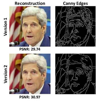
Figure 5: Demonstrating the differences between Versions 1 and 2 on super resolution ($4\times$). The two columns show the reconstructions with PSNRs and their corresponding “canny edges”, respectively.

Surprisingly, we observe that MCG seems to have a lot of variability in the results on the LSUN-Bedroom dataset, but performs well on FFHQ (shown in Appendix B). This might suggest that datasets such as faces are generally easier than datasets with more complicated structures such as bedrooms.

For the results with CMs, we present the quantitative results in Table 1 and  Table 2 highlighted in orange, with visual results in Figure 6. This highlights another use case of our algorithm, as it demonstrates that our algorithm can flexibly utilize CMs compared to existing methods.

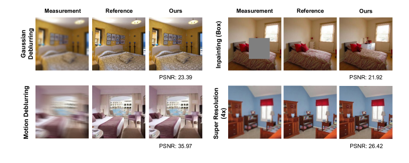
Figure 6: Qualitative results for various image restoration problems by using CMs. Our proposed framework is capable of utilizing CMs for image restoration.

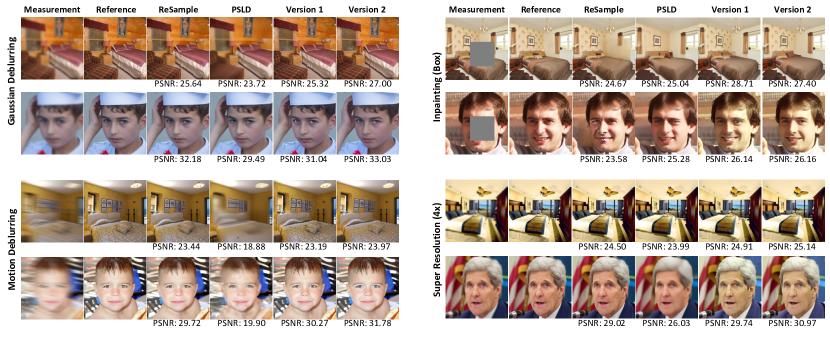
Figure 7: Latent space diffusion models for solving various image restoration problems. These results demonstrate the effectiveness of our algorithm. We can consistently recover images with the highest PSNR.

5.2.2 Latent Space Diffusion Models

For the results with LDMs, we display quantitative results in Table 1 and Table 2 highlighted in blue, with qualitative results in Figure 7. Recall that as outlined in Section 4.2, there are two approaches for ensuring data consistency. For the best performance, we use pixel space optimization (Approach 2) for motion deblurring and Gaussian deblurring and latent space optimization (Approach 1) for box inpainting and super-resolution. As observed in the tables, we observe that our algorithm outperforms the existing baselines on many of the inverse problems. Interestingly, we observe that PSLD seems to reconstruct images that are often noisy and blurry, where the learning rate plays a huge role on the reconstruction quality. While ReSample may have higher LPIPS scores on some inverse problem tasks, our algorithm is able to achieve better PSNR and SSIM scores.

5.3 Ablation Studies

Finally, we conduct ablation studies demonstrating computational efficiency, convergence, and robustness to measurement noise.

Computational Efficiency.

First, we compare the inference times (the time it takes to reconstruct a single image) of our method with the baselines and display the results in Table 3. Clearly, for pixel based diffusion models, our methods are much more efficient than DPS [16] and MCG [13], as we do not require backpropogation through the score function for data consistency. Furthermore, using the single step Tweedie’s formula approximation for diffusion purification is much faster than using reverse SDE which involves multiple time steps.

Second, for latent space methods, our methods are also faster than existing methods PSLD [20] and ReSample [21] as observed in Table 3. For our own methods, we observe that optimizing at the pixel level (Approach 2) for data consistency proves to be considerably more efficient than optimizing in the latent space (Approach 1). As previously mentioned, this is due to the need for backpropagating through the complex deep decoder $\mathcal{D}(\cdot)$. This is also one of the main reasons our methods are more computationally efficient than methods such as ReSample.

Algorithm	Time (sec)
DPS [16]	387
MCG [13]	385
Our Pixel (Reverse SDE, Version 1)	28.7
Our Pixel (Tweedie’s Formula, Version 2)	2.14
PSLD [20]	188
ReSample [21]	118
Our Latent (Latent DC + Reverse SDE)	109
Our Latent (Pixel DC + Reverse SDE)	12.2
Our Latent (Latent DC + Tweedie’s Formula)	100
Our Latent (Pixel DC + Tweedie’s Formula)	2.59

Table 3: Comparison of inference times. The results colored in blue are for LDMs, whereas the others are for pixel space diffusion models.

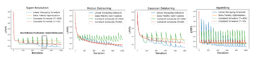
Figure 8: Convergence of our methods in terms of LPIPS. The orange, green, red and blue curves correspond to the reconstruction process with data fidelity optimization only, our proposed method with a constant (large) purification strength, constant (small) purification strength and a linear decaying purificaiton strength, respectively. The x-axis denotes the total number of data fidelity gradient steps.

Convergence Study.

In this section, we investigate the convergence of our algorithm in terms of LPIPS. This study also serves to demonstrate the efficiency of a linear decaying time schedule for $T_{k}$ for diffusion purification across various image restoration problems. As shown in Figure 8, at the beginning of each diffusion purification and data fidelity optimization cycle, the LPIPS increases after performing diffusion purification due to stochasticity introduced by the forward-backward diffusion process. However, the subsequent iterations can successfully decrease LPIPS and result in reconstructions with higher qualities compared to pure data fidelity optimization, illustrating that the resulting purified image is able to serve as a good initialization point. In the same figure, also notice that the linear decaying schedule greatly enhances the performance of our algorithm compared to using a constant time schedule for $T_{k}$. This is expected, as a large constant purification strength will result in serious hallucination while a small constant purification strength is not able to fully alleviate the artifacts in the data fidelity based estimations. In Figure 9, we illustrate an example reconstruction process for super-resolution with noisy measurements, with more examples in the Appendix. It is evident that the quality of the reconstructed image gradually increases with more iterations.

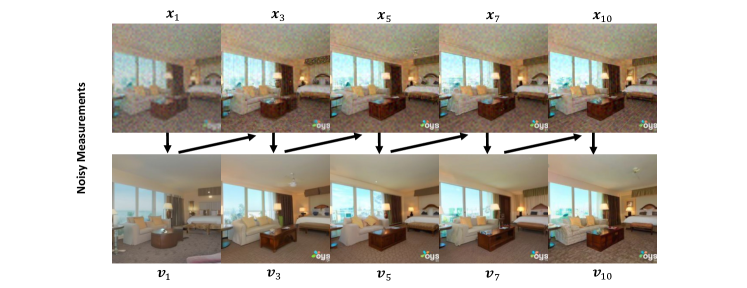
Figure 9: Reconstruction process for super-resolution (4x) in the pixel space. To compensate the artifacts introduced by the measurement noise, the reconstruction process takes $K=10$ iterations in total with a time schedule starting at $T_{1}=400$ and linearly decaying to $T_{10}=200$. The learning rate for data fidelity optimization is $lr=100$.

		Super Resolution ($4\times$)			Motion Deblurring
Metric		DPS [16]	Version 1	Version 2	DPS [16]	Version 1	Version 2
($\sigma_{\bm{y}}=0.050$)	LPIPS$\downarrow$	$\mathbf{0.287}\pm 0.03$	$\underline{0.321}\pm 0.05$	$0.363\pm 0.05$	$\mathbf{0.328}\pm 0.07$	$\underline{0.332}\pm 0.05$	$0.361\pm 0.05$
	PSNR$\uparrow$	$\underline{24.50}\pm 2.88$	$24.23\pm 2.45$	$\mathbf{24.66}\pm 2.55$	$22.43\pm 2.83$	$\underline{23.47}\pm 2.23$	$\mathbf{24.18}\pm 2.31$
	SSIM$\uparrow$	$\underline{0.697}\pm 0.08$	$0.687\pm 0.09$	$\mathbf{0.709}\pm 0.09$	$0.642\pm 0.09$	$\underline{0.669}\pm 0.09$	$\mathbf{0.703}\pm 0.09$
($\sigma_{\bm{y}}=0.075$)	LPIPS$\downarrow$	$\underline{0.342}\pm 0.04$	$\mathbf{0.325}\pm 0.05$	$0.363\pm 0.05$	$\underline{0.343}\pm 0.07$	$\mathbf{0.340}\pm 0.05$	$0.357\pm 0.05$
	PSNR$\uparrow$	$23.72\pm 2.59$	$\underline{24.12}\pm 2.41$	$\mathbf{24.62}\pm 2.54$	$22.09\pm 2.77$	$\underline{23.17}\pm 2.20$	$\mathbf{24.13}\pm 2.29$
	SSIM$\uparrow$	$0.644\pm 0.08$	$\underline{0.681}\pm 0.09$	$\mathbf{0.709}\pm 0.09$	$0.623\pm 0.11$	$\underline{0.649}\pm 0.09$	$\mathbf{0.699}\pm 0.09$
($\sigma_{\bm{y}}=0.100$)	LPIPS$\downarrow$	$0.393\pm 0.04$	$\mathbf{0.339}\pm 0.05$	$\underline{0.362}\pm 0.05$	$\mathbf{0.352}\pm 0.07$	$0.378\pm 0.05$	$\underline{0.368}\pm 0.05$
	PSNR$\uparrow$	$22.85\pm 2.39$	$\underline{23.92}\pm 2.34$	$\mathbf{24.57}\pm 2.52$	$21.76\pm 2.70$	$\underline{22.49}\pm 2.06$	$\mathbf{24.05}\pm 2.26$
	SSIM$\uparrow$	$2.584\pm 0.08$	$\underline{0.668}\pm 0.08$	$\mathbf{0.707}\pm 0.09$	$\underline{0.614}\pm 0.11$	$0.593\pm 0.09$	$\mathbf{0.690}\pm 0.09$

Table 4: Case study of noise robustness of our methods compared to DPS on two image restoration problems in the pixel space. We compare our algorithm to DPS on super resolution ($4\times$) and motion deblurring to demonstrate that our method is effective even in the presence of measurement noise. Best results are bolded and second best results are underlined.

Noise Robustness.

Thus far, we considered experiments on image restoration tasks in which the measurements were noiseless. However, in many practical settings of interest, the measurements $\bm{y}$ can be corrupted with additive noise. In this section, we perform an ablation study on the performance of our algorithm in which the measurements have additive Gaussian noise $\mathcal{N}(0,\sigma^{2}_{\bm{y}})$, with varying values of $\sigma_{\bm{y}}$ for super resolution and motion deblurring. We compare our algorithm to DPS, as their theory states that the approximation of their gradient likelihood term actually becomes tighter as the measurement noise $\sigma_{\bm{y}}$ increases [16]. We conduct experiments on $100$ randomly selected images from the LSUN-Bedroom dataset for super-resolution, motion deblurring on standard deviations $0.05,0.075$, and $0.1$. For the hyperparameters, we tune the parameters according to $\sigma_{\bm{y}}=0.01$ and fix them throughout the experiments. The rest of the setup is the same as previously described. We present the results in Table 4. Here we observe that as the standard deviation increases, the performance of all algorithms slightly degrades, as expected. However, our algorithm consistently outperforms DPS in metrics such as PSNR and SSIM, whereas DPS often exhibits higher perceptual quality measured by LPIPS. This difference arises because DPS frequently suffers from hallucinations, introducing artifacts in the image that “sharpen” it. Our algorithm is less susceptible to such artifacts, resulting in “smoother” images with higher signal-to-noise ratios. Details of the hyperparameters and visual results can be found in Section A.3.

6 Relationship to Prior Arts

Here, we discuss the relationship of our work with existing methods for image restoration, including both methods derived in the pixel space and algorithms tailored for the latent space.

Pixel Space Diffusion Models.

Other than DPS [16], there are other diffusion model-based inverse problem solvers available for addressing image restoration tasks. Song et al. [17] introduced $\Pi$GDM, an algorithm that approximates the likelihood gradient using a pseudo-inverse of the linear sensing matrix used for generating the measurements. When the operator $\mathcal{A}(\cdot)$ is linear, it can be represented by a matrix $\bm{A}\in\mathbb{R}^{m\times n}$, for which one can calculate its pseudo-inverse. They leverage this property by first constructing the conditional distribution $p(\bm{y}|\bm{x}_{t})$ in terms of the sensing matrix $\bm{A}$ and derive the likelihood gradient using this conditional distribution. The work by Wang et al. [15] has a similar flavor; since the image restoration problem is ill-posed, the reconstructions without priors generally are a mixture of a sample in both the range and the nullspace of the matrix $\bm{A}$. They use the diffusion model as a prior to essentially “fill in” this nullspace, which is constructed by taking the pseudo-inverse of $\bm{A}$ and used during the reverse sampling process. The work presented in [50] introduced the Direct Diffusion Bridge method building upon the DPS approach. Here, the data fidelity is enforced during the reverse sampling procedure by taking a deeper gradient step which is designed for improved data consistency.

Another popular method for addressing image restoration problems is the Denoising Diffusion Restoration Models (DDRMs) proposed by Kawar et al. [51]. DDRMs construct a probabilistic graph conditioned on the measurements, allowing the use of a pre-trained unconditional diffusion model. Subsequently, they perform the reverse sampling process in the “spectral space”, which is constructed by taking the SVD of the sensing matrix $\bm{A}$. These works generally share two common themes: they require the inverse problem to be linear, and they incorporate the data consistency steps in the reverse diffusion process. Although we do not test on nonlinear inverse problems, our algorithm does not face these limitations and is flexible in this regard.

Lastly, the study presented by Luther et al. [52] shares close ties with Version 2 our algorithm in the pixel space. They introduced Diffusive Denoising of Gradient-based Minimization (DDGM), an image-space method for solving linear tomographic reconstruction problems, which iteratively applies data consistency steps and image denoising through a pre-trained diffusion model. However, as we have shown in Section 5.2, directly regularizing images with Tweedie’s formula will result in blurry images. In contrast, the proposed Version 1 of our algorithm alleviates this issue by performing diffusion purification with multiple diffusion reverse sampling steps. Furthermore, we propose a unified framework that can incorporate accelerated samplers, latent diffusion models, and consistency models, thereby significantly reducing the inference time. Hence, our work addresses a broader spectrum, not only limited to tomographic reconstruction, and can be readily adapted to applications requiring fast inference.

Latent Space Diffusion Models.

Throughout our experiments, we also presented results using LDMs, using PSLD [20] and ReSample [21] as baselines. ReSample [21] is an algorithm designed to solve inverse problems in the latent space that involves solving a data fidelity optimization problem during the reverse sampling process, a process they term “hard data consistency”. The data fidelity objective is similar to the approaches we take, where they alternate between minimizing the objective in either the latent space or the pixel space. Upon solving this objective, they devise a resampling scheme to project the data-consistent sample back onto the noisy manifold to continue the reverse sampling process. Nonetheless, by decoupling these two processes, our algorithm does not require a resampling stage. Additionally, ReSample cannot use accelerated samplers because of the coupling, as it would hinder the data fidelity stage by reducing the number of sampling steps, unlike our framework.

Posterior Sampling with Latent Diffusion (PSLD) [20] extends the idea of DPS to the latent space by addressing the challenge that the decoder and encoder constitute a many-to-one mapping. This implies that there may be multiple latent codes that fit the measurements, and they devise a gradient scheme to ensure the “correct” latent code is estimated during the reverse sampling process. However, their technique involves two gradient computations—one through the LDM decoder and one through the pre-trained LDM score function. Thus, PSLD suffers from increased inference time. Furthermore, it is observed in our experiment that the performance of PSLD is sensitive to the choice of hyperparameters.

Plug-and-Play (PnP) Methods.

The Plug-and-Play Priors (PnP) framework combines physical and learned models for effective computational imaging. PnP alternates between minimizing a data-fidelity term for enforcing data consistency and applying a learned regularizer, typically an image denoiser [53, 36, 37]. The PnP framework is commonly formulated using the Alternating direction method of multipliers (ADMM) [36] and fast iterative shrinkage/thresholding algorithms (FISTA) [54]. Our proposed method shares similarity with the PnP in the sense that both methods utilize image denoisers as the implicit prior. However, while PnP performs denoising directly on $\bm{x}_{k}$ by assuming that $\bm{x}_{k}$ contains certain pseudo noise, our proposed method uses diffusion models to explicitly add noise to $\bm{x}_{k}$ and then denoises it by either iterative sampling or Tweedie’s formula [52] estimation.

7 Discussion & Conclusion

Throughout this paper, we have discussed both the efficiency and flexibility of our algorithm, demonstrating that we can compete with many state-of-the-art techniques while offering numerous advantages. However, despite these strengths, our algorithm has a few steps that warrant further investigation. Recall that the input to the diffusion purification stage is an initial reconstruction estimated from minimizing the data fidelity objective. Notice that if this step does not return an estimate that is meaningful, then the diffusion purification stage cannot produce a high-quality reconstruction. Although this was not an issue for the image restoration problem that we considered, it may be the case for more complex problems, as simply minimizing the data fidelity objective in Equation (10) can lead to poor local minima. For these tasks, it would be of great interest to explore replacing Equation (10) with more advanced solvers.

Furthermore, while our algorithm generally outperforms others in metrics such as PSNR and SSIM, it often only shows marginal improvements in LPIPS, which measures perceptual quality. This outcome is expected, as coupled methods like DPS prioritize the prior step more meticulously, potentially leading to hallucinations. On the other hand, by decoupling data fidelity from the prior, our algorithm places greater emphasis on data fidelity. Therefore, exploring methods to carefully balance between the prior and data consistency with decoupling is an important avenue for future research.

8 Data Availability Statement

The code and instructions for reproducing the experiment results will be made available in the following link: https://github.com/Morefre/Decoupled-Data-Consistency-with-Diffusion-Purification-for-Image-Restoration.

Appendix A Implementation Details

Notation	Definition
$K\in\mathbb{N}$	Number of iterations for overall algorithm
$\tau\in\mathbb{N}$	Total number of iterations for data consistency optimization
$\alpha\in\mathbb{R}$	Learning rate for data consistency optimization
$T_{k}\in\mathbb{R}$	Diffusion purification strength at the $k^{\text{th}}$ iteration
$\bm{v}_{k}\in\mathbb{R}^{n}$	Prior consistent sample at $k^{\text{th}}$ iteration
$\bm{x}_{k}\in\mathbb{R}^{n}$	Data consistent sample at $k^{\text{th}}$ iteration

Table 5: Summary of the notation used throughout this work.

A.1 Discussion on Hyperparameters

Here, we discuss the hyperparameters associated with our algorithm and some typical choices we made throughout our experiments.

• Total Number of Iterations. We run the algorithm for a total of $K$ iterations, which refers to reconstructing the image by alternately applying data fidelity optimization and diffusion purification for $K$ rounds. Empirically, we observe a $K$ ranging from 10 to 20 is sufficient for generating high quality reconstructions. We suggest users start with $K=10$ and then gradually decrease it if a faster computation speed is required.

• Optimizer for Data Fidelity Optimization. Throughout our experiments, we use momentum-based gradient descent with the momentum hyperparameter set to 0.9. The optimal learning rate (LR) for data fidelity optimization varies from task to task. In general, the LR should neither be too large, which will not result in images with meaningful structures, nor too small, in which case the convergence speed of the overall algorithm will be too slow. Throughout the experiment we fix the number of gradient steps for each round of the data fidelity optimization. When the measurements are corrupted by noise, one can further perform early stopping to prevent overfitting to the noise.

• Decaying Time Schedule for Diffusion Purification. A decaying time schedule plays the key role in the success of our proposed algorithm. As described in  Section 3.3, given a data fidelity based reconstruction $\bm{x}_{k}$, the goal of diffusion purification is to generate $\bm{v}_{k}$ that shares the overall structural and semantic information of $\bm{x}_{k}$, such that it is consistent with the measurements while at the same time being free from the artifacts visible in $\bm{x}_{k}$. Unfortunately, the $\bm{v}_{k}$ resulting from diffusion purification is sensitive to the choice of $T$, i.e., the amount of noise added to $\bm{x}_{k}$. When $T$ is small, the resulting $\bm{v}_{k}$ will exhibit similar structure to $\bm{x}_{k}$ but with artifacts, as there is not enough noise to submerge these artifacts through diffusion purification. On the other hand, when $T$ is too large, though $\bm{v}_{k}$ will be free from artifacts, its semantic information and overall structure will significantly deviate from $\bm{x}_{k}$. As a result, the resulting reconstructions will not be measurement-consistent.

  To this end, previous works that utilize diffusion purification [31, 14] depend on fine-tuning an optimal $T^{\star}$. However, we find that the fine-tuning strategy can be infeasible since the optimal $T^{\star}$ varies from task to task and even from image to image. To alleviate the need to identify the optimal $T^{\star}$, we implement a linear decaying schedule $\{T_{k}\}_{k\in[K]}$ for each iteration $k$. In the early iterations when $T_{k}$ is relatively large, the resulting $\bm{v}_{k}$, though inconsistent with the measurements, will be free from artifacts and can serve as good starting point for the subsequent iteration of data fidelity optimization. As $T_{k}$ keeps decreasing, the algorithm will converge at an equilibrium point which is both consistent with the measurements and free from the artifacts. When the measurements are noiseless, we observe that for a diffusion model trained with 1000 total timesteps, a linear decaying time schedule starting from $T_{1}=400$ and ending at $T_{K}=0$ results in reconstructions with high quality for Super-Resolution, Gaussian Deblurring and Motion Deblurring. For Box Inpainting, we choose a higher initial timestep $T_{1}=700$ and $T_{1}=500$ for pixel space diffusion models and LDMs respectively to compensate the severe artifacts in the large box region. When the measurements are corrupted by noise, one may instead end at $T_{K}=T$, where $T>0$ to compensate the negative effect of the measurement noise. We demonstrate the reconstruction process for various tasks in Figures 10, 11, 12, 13 and 16. Notice that the diffusion purification removes the artifacts from the initial reconstructions obtained via data fidelity optimization especially in the early iterations and results in high quality reconstructions consistent with the measurements as timestep decreases.

  

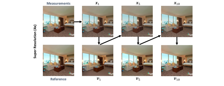
  Figure 10: Reconstruction process for super-resolution with pixel space diffusion models. The reconstruction process takes $K=10$ iterations in total with a time schedule starting at $T_{1}=400$ and linearly decaying to $T_{10}=0$. We demonstrate reconstructions at timesteps 1, 5, and 10.

  

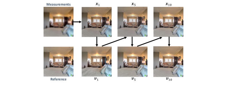
  Figure 11: Reconstruction Process for Gaussian Deblurring with Pixel Space Diffusion Models. The reconstruction process takes $K=10$ iterations in total with a time schedule starting at $T_{1}=400$ and linearly decaying to $T_{10}=0$. Due to the space limit, only reconstructions at timesteps 1, 5 and 10 are shown.

  

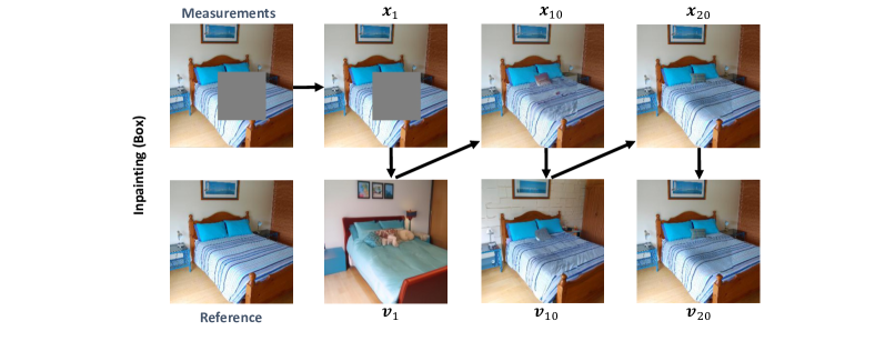
  Figure 12: Reconstruction Process for Inpainting with Pixel Space Diffusion Models. The reconstruction process takes $K=20$ iterations in total with a time schedule starting at $T_{1}=700$ and linearly decaying to $T_{20}=0$. Due to the space limit, only reconstructions at timesteps 1, 10 and 20 are shown.

  

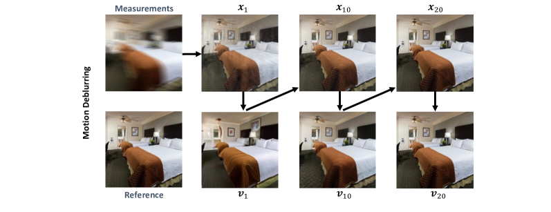
  Figure 13: Reconstruction Process for Motion Deblurring with Pixel Space Diffusion Models. The reconstruction process takes $K=20$ iterations in total with a time schedule starting at $T_{1}=400$ and linearly decaying to $T_{20}=0$. Due to the space limit, only reconstructions at timesteps 1, 10 and 20 are shown.

• DDIM Steps for Diffusion Purification. With the help of accelerated diffusion samplers such as DDIMs [11], we can perform diffusion purification with as low as 20 unconditional sampling steps. As mentioned before, the total number of iterations $K$ ranging from 10-20 is sufficient for generating high quality reconstructions. This amounts to 200 to 400 unconditional reverse sampling steps in total, a significantly lower figure compared to DPS [16], which requires 1000 unconditional reverse sampling steps. Interestingly, we find that increasing the DDIM sampling steps does not necessarily improve the performance of diffusion purification. Therefore, we suggest users use 20 steps for diffusion purification.

• Pixel Space Optimization and Latent Space Optimization. As discussed in Section 4.2, in the case of LDMs, one can use either Pixel Space Optimization Equation (20) or Latent Space Optimization (18) to enforce the data consistency. Depending on the specific task, one approach may generate $\bm{x}_{k}$’s with higher quality than the other. In practice, as shown in Figures 14 and 15, we observe that for motion deblurring and Gaussian deblurring, the initial reconstructions generated with Pixel Space Optimization have significantly higher quality compared to the ones generated with Latent Space Optimization. Furthermore, Pixel Space Optimization is much faster than the Latent Space Optimization since the gradient computation of the former approach does not require backpropagation through the deep decoder $\mathcal{D}(\cdot)$. To achieve the best reconstruction quality, we suggest users try both options and choose the one which gives the best performance. On the other hand, for applications that require fast reconstruction speed, we suggest using Pixel Space Optimization.

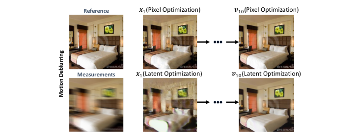
Figure 14: Comparison between Pixel Space Optimization and Latent Space Optimization for Motion Deblurring. Initial Reconstructions obtained via Pixel Space Pptimization have much better quality compared to the ones obtained from Latent Space Optimization which in turn result in final reconstructions with higher quality.

A.2 Choice of Hyperparameters

In this section, we specify the hyperparameters used for generating the results in Section 5. For the baselines, we either followed the instructions given in each respective work or used the parameters provided in their code.

A.2.1 Experiments with Pixel Space Diffusion Models

For the hyperparameters used for the pixel space experiments, we tabulate all of our values for each dataset in Table 6. Recall that for $T_{k}$, we choose a linearly decaying time schedule. We start at a value $T_{0}$, which is specified in the table. For box inpainting, we used a larger value of $T_{0}$ to compensate for the large artifacts that exist within the box region. The diffusion purification is performed with 20 deterministic DDIM steps.

We optimize the data fidelity objective with momentum-based gradient descent with the momentum hyperparameter set to $0.9$ for both FFHQ and LSUN-Bedrooms datasets. To achieve the best performance, we use Pixel Space Optimization for Gaussian deblurring and motion deblurring while using Latent Space Optimization for box inpainting and super-resolution. Again, we fix the total number of gradient steps as 1000 throughout the $K$ iterations, which means we take $\frac{1000}{K}$ gradient steps in each round of data fidelity optimization.

Dataset	Super Resolution ($4\times$)			Gaussian Deblurring			Motion Deblurring			Inpainting (Box)
	$\alpha$	$K$	$T_{0}$	$\alpha$	$K$	$T_{0}$	$\alpha$	$K$	$T_{0}$	$\alpha$	$K$	$T_{0}$
LSUN-Bedrooms	$10^{3}$	$10$	$400$	$10^{5}$	$10$	$400$	$10^{5}$	$20$	$400$	$10^{3}$	$20$	$700$
FFHQ	$10^{3}$	10	$400$	$10^{5}$	$10$	$400$	$10^{5}$	$20$	$400$	$10^{3}$	$20$	$700$

Table 6: Table of hyperparameters used for experiments in the pixel space. $\alpha$ refers to the learning rate used in the data consistency optimization, $K$ refers to the total number of iterations, and $T_{0}$ refers to the starting point for the linearly decaying time schedule.

Dataset	Super Resolution ($4\times$)			Gaussian Deblurring			Motion Deblurring			Inpainting (Box)
	$\alpha$	$K$	$T_{0}$	$\alpha$	$K$	$T_{0}$	$\alpha$	$K$	$T_{0}$	$\alpha$	$K$	$T_{0}$
LSUN-Bedrooms	$10^{3}$	$10$	$400$	$10^{5}$	$10$	$400$	$10^{5}$	$10$	$400$	$10^{3}$	$20$	$500$
FFHQ	$10^{3}$	$10$	$400$	$10^{5}$	$10$	$400$	$10^{5}$	$4$	$400$	$10^{3}$	$20$	$500$

Table 7: Table of hyperparameters used for experiments in the latent space. $\alpha$ refers to the learning rate used in the data consistency optimization, $K$ refers to the total number of iterations, and $T_{0}$ refers to the starting point for the linearly decaying time schedule.

Dataset	Super Resolution ($4\times$)			Gaussian Deblurring			Motion Deblurring			Inpainting (Box)
	$\alpha$	$K$	$T_{0}$	$\alpha$	$K$	$T_{0}$	$\alpha$	$K$	$T_{0}$	$\alpha$	$K$	$T_{0}$
LSUN-Bedrooms	$10^{3}$	$20$	$1$	$10^{5}$	$20$	$1$	$10^{5}$	$20$	$1$	$10^{3}$	$20$	$5$

Table 8: Table of hyperparameters used for experiments with CMs. $\alpha$ refers to the learning rate used in the data consistency optimization, $K$ refers to the total number of iterations, and $T_{0}$ refers to the starting point for the linearly decaying time schedule. Different from the typical diffusion models used in previous experiments which use a noise scale in the range of [0,1000], CMs are trained in the range of [0.002,80].

Method	Super Resolution $4\times$			Inpainting (Box)
	LPIPS$\downarrow$	PSNR$\uparrow$	SSIM$\uparrow$	LPIPS$\downarrow$	PSNR$\uparrow$	SSIM$\uparrow$
DPS [16]	$\underline{0.176}$ $\pm 0.04$	$28.45\pm 1.99$	$0.792\pm 0.05$	$0.115\pm 0.02$	$23.14\pm 3.14$	$0.829\pm 0.03$
MCG [13]	$0.182\pm 0.03$	$24.45\pm 2.93$	$0.736\pm 0.06$	$0.119\pm 0.02$	$22.77\pm 3.06$	$0.827\pm 0.03$
ADMM-PnP [47]	$0.307\pm 0.03$	$21.54\pm 3.12$	$0.766\pm 0.03$	$0.251\pm 0.02$	$18.26\pm 1.86$	$0.724\pm 0.02$
Ours Pixel (Version 1)	$\bm{0.154}\pm 0.03$	$\underline{29.43}\pm 2.01$	$\underline{0.844}\pm 0.03$	$\underline{0.052}\pm 0.01$	$\underline{25.54}\pm 3.01$	$\underline{0.917}\pm 0.01$
Ours Pixel (Version 2)	$0.185\pm 0.03$	$\bm{30.86}\pm 2.11$	$\bm{0.878}\pm 0.03$	$\bm{0.051}\pm 0.01$	$\bm{28.02}\pm 2.74$	$\bm{0.935}\pm 0.01$
PSLD [20]	$0.309\pm 0.06$	$26.22\pm 2.07$	$0.758\pm 0.06$	$0.248\pm 0.06$	$25.42\pm 2.15$	$0.788\pm 0.05$
Ours LDMs (Version 1)	$\bm{0.183}\pm 0.04$	$\underline{29.16}\pm 1.65$	$\underline{0.826}\pm 0.03$	$\bm{0.166}\pm 0.03$	$\underline{26.50}\pm 2.20$	$\underline{0.860}\pm 0.02$
Ours LDMs (Version 2)	$\underline{0.215}\pm 0.04$	$\bm{30.61}\pm 1.97$	$\bm{0.866}\pm 0.03$	$\underline{0.204}\pm 0.04$	$\bm{27.47}\pm 2.05$	$\bm{0.868}\pm 0.03$

Table 9: Quantitative results of super resolution and inpainting on the FFHQ dataset for both pixel-based and LDMs. The results colored in blue are for LDMs, while the others are for pixel space diffusion models. The Best Results are in bold and second best results are underlined for pixel space models and LDMs respectively.

Method	Gaussian Deblurring			Motion Deblurring
	LPIPS$\downarrow$	PSNR$\uparrow$	SSIM$\uparrow$	LPIPS$\downarrow$	PSNR$\uparrow$	SSIM$\uparrow$
DPS [16]	$\underline{0.162}\pm 0.03$	$27.97\pm 2.01$	$0.782\pm 0.05$	$0.219\pm 0.04$	$25.34\pm 2.21$	$0.690\pm 0.07$
MCG [13]	$0.164\pm 0.03$	$25.03\pm 3.62$	$0.790\pm 0.06$	$0.343\pm 0.04$	$24.88\pm 2.01$	$0.708\pm 0.05$
ADMM-PnP [47]	$0.421\pm 0.03$	$20.86\pm 2.16$	$0.664\pm 0.05$	$0.522\pm 0.02$	$17.91\pm 1.99$	$0.547\pm 0.06$
Ours Pixel (Version 1)	$\bm{0.140}\pm 0.02$	$\underline{30.41}\pm 1.93$	$\underline{0.864}\pm 0.03$	$\bm{0.051}\pm 0.01$	$\underline{37.56}\pm 1.77$	$\underline{0.963}\pm 0.01$
Ours Pixel (Version 2)	$0.173\pm 0.03$	$\bm{31.67}\pm 2.12$	$\bm{0.891}\pm 0.03$	$\underline{0.060}\pm 0.01$	$\bm{38.37}\pm 1.88$	$\bm{0.970}\pm 0.01$
PSLD [20]	$0.270\pm 0.05$	$27.46\pm 1.84$	$0.790\pm 0.05$	$0.379\pm 0.05$	$22.35\pm 1.85$	$0.641\pm 0.07$
Ours LDMs (Version 1)	$\underline{0.198}\pm 0.03$	$\underline{28.91}\pm 1.98$	$\underline{0.825}\pm 0.04$	$\underline{0.152}\pm 0.03$	$\underline{30.11}\pm 1.93$	$\underline{0.851}\pm 0.03$
Ours LDMs (Version 2)	$\bm{0.171}\pm 0.02$	$\bm{30.45}\pm 1.86$	$\bm{0.877}\pm 0.03$	$\bm{0.108}\pm 0.02$	$\bm{31.48}\pm 1.94$	$\bm{0.894}\pm 0.02$

Table 10: Quantitative results of Gaussian and motion deblurring on the FFHQ dataset for both pixel-based and LDMs. The results colored in blue are for LDMs, while the others are for pixel space diffusion models. The Best Results are in bold and second best results are underlined for pixel space models and LDMs respectively.

A.2.2 Experiments with LDMs

Similarly, we specify the hyperparameters used for experiments using LDMs in Table 7. For box inpainting, similar to the pixel space experiments, we used a larger value of $T_{0}$ to compensate for the artifacts seen in the box region. The diffusion purification is performed with 20 deterministic DDIM steps. For the data fidelity objectives, the same procedure done in the pixel space was applied for the LDM case.

A.2.3 Experiments with CMs

Lastly, we specify the hyperparameters used for experiments using CMs in Table 8. Notice that different from the typical diffusion model used previously which use a noise scale in the range of [0,1000], CMs are traind in the range of [0.002,80]. Again, the diffusion purification is performed with 20 deterministic DDIM steps.

A.3 Dealing with Measurement Noise

When the measurements are noiseless, a linear decaying schedule starts from $T_{0}$ and ends at $T_{K}=0$ is capable of resulting in high quality reconstructions and we can use a relatively high learning rate for the data fidelity optimization. On the contrary, in the presence of measurement noise, the data fidelity optimization in (10) will inevitably introduce additional artifacts even if $\bm{v}_{k-1}$ is the ground truth image. To achieve robust recovery, one may instead: (i) use a relatively small learning rate for data fidelity optimization to prevent overfitting to the noise, and (ii) end the time schedule at $t_{K}=T$, where $T>0$, to compensate for the artifacts resulting from the measurement noise. As shown in  Figure 16, compared to the clean measurements case, due to the additive noise, the data fidelity optimization always introduce artifacts in $\bm{x}_{k}$. This issue can be alleviated by utilizing a non-zero diffusion purification strength at the final iteration. For the experiments in Section 5.3, all the hyperparameters are kept the same as described in Section A.2.1, but with the following changes:

• The learning rate for motion deblurring changes from $1e^{5}$ to $1e^{4}$.

• The time schedules for super-resolution and motion deblurring start from $t_{0}=400$ and decay linearly to $250$ and $300$ respectively.

With the changes made above, our algorithm achieves reconstruction performance comparable to that of DPS with measurement noise. Notice that the hyperparameters are chosen such that they work under the most severe noise level, i.e., $\sigma=0.1$. Better performance can be achieved by decreasing $t_{K}$ in the case of $\sigma=0.05$ or $\sigma=0.075$.

Appendix B Additional Quantitative Results

In this section, we provide additional quantitative results for solving inverse problems on the FFHQ dataset. The results are presented in Tables 9 and 10. Throughout all of our experiments, we observe that our proposed algorithms outperform the baselines for various image restoration problems.

(a) Reference and Measurements for Super-Resolution (4x). The noisy measurements are corrupted by random Gaussian noise with $\sigma=0.1.$

(b) Reconstruction Process with Clean Measurements. The reconstruction process takes $K=10$ iterations in total with a time schedule starting at $T_{1}=400$ and linearly decaying to $T_{10}=0$. The learning rate for data fidelity optimization is $lr=1000$. Due to the space limit, only reconstructions at timesteps 1, 3, 5, 7 and 10 are shown.

(c) Reconstruction Process with Noisy Measurements. To compensate the artifacts introduced by the measurement noise, the reconstruction process takes $K=10$ iterations in total with a time schedule starting at $T_{1}=400$ and linearly decaying to $T_{10}=200$. The learning rate for data fidelity optimization is $lr=100$.

Figure 16: Reconstruction Process for Super-Resolution (4x) with Pixel Space Diffusion Models.

References

- [1] Gregory Ongie, Ajil Jalal, Christopher A Metzler, Richard G Baraniuk, Alexandros G Dimakis, and Rebecca Willett. Deep learning techniques for inverse problems in imaging. IEEE Journal on Selected Areas in Information Theory, 1(1):39–56, 2020.
- [2] Saiprasad Ravishankar, Jong Chul Ye, and Jeffrey A Fessler. Image reconstruction: From sparsity to data-adaptive methods and machine learning. Proceedings of the IEEE, 108(1):86–109, 2019.
- [3] Jure Zbontar, Florian Knoll, Anuroop Sriram, Tullie Murrell, Zhengnan Huang, Matthew J Muckley, Aaron Defazio, Ruben Stern, Patricia Johnson, Mary Bruno, et al. fastmri: An open dataset and benchmarks for accelerated mri. arXiv preprint arXiv:1811.08839, 2018.
- [4] Ashish Bora, Ajil Jalal, Eric Price, and Alexandros G Dimakis. Compressed sensing using generative models. In International conference on machine learning, pages 537–546. PMLR, 2017.
- [5] Jay Whang, Qi Lei, and Alex Dimakis. Solving inverse problems with a flow-based noise model. In International Conference on Machine Learning, pages 11146–11157. PMLR, 2021.
- [6] Mario González, Andrés Almansa, and Pauline Tan. Solving inverse problems by joint posterior maximization with autoencoding prior. SIAM Journal on Imaging Sciences, 15(2):822–859, 2022.
- [7] Dmitry Ulyanov, Andrea Vedaldi, and Victor Lempitsky. Deep image prior. In Proceedings of the IEEE conference on computer vision and pattern recognition, pages 9446–9454, 2018.
- [8] Jonathan Ho, Ajay Jain, and Pieter Abbeel. Denoising diffusion probabilistic models. Advances in neural information processing systems, 33:6840–6851, 2020.
- [9] Yang Song, Jascha Sohl-Dickstein, Diederik P Kingma, Abhishek Kumar, Stefano Ermon, and Ben Poole. Score-based generative modeling through stochastic differential equations. In International Conference on Learning Representations, 2020.
- [10] Prafulla Dhariwal and Alexander Nichol. Diffusion models beat gans on image synthesis. Advances in neural information processing systems, 34:8780–8794, 2021.
- [11] Jiaming Song, Chenlin Meng, and Stefano Ermon. Denoising diffusion implicit models. In International Conference on Learning Representations, 2020.
- [12] Hyungjin Chung, Byeongsu Sim, and Jong Chul Ye. Come-closer-diffuse-faster: Accelerating conditional diffusion models for inverse problems through stochastic contraction. In Proceedings of the IEEE/CVF Conference on Computer Vision and Pattern Recognition, pages 12413–12422, 2022.
- [13] Hyungjin Chung, Byeongsu Sim, Dohoon Ryu, and Jong Chul Ye. Improving diffusion models for inverse problems using manifold constraints. Advances in Neural Information Processing Systems, 35:25683–25696, 2022.
- [14] Jooyoung Choi, Sungwon Kim, Yonghyun Jeong, Youngjune Gwon, and Sungroh Yoon. Ilvr: Conditioning method for denoising diffusion probabilistic models. In 2021 IEEE/CVF International Conference on Computer Vision (ICCV), pages 14347–14356. IEEE, 2021.
- [15] Yinhuai Wang, Jiwen Yu, and Jian Zhang. Zero-shot image restoration using denoising diffusion null-space model. In The Eleventh International Conference on Learning Representations, 2022.
- [16] Hyungjin Chung, Jeongsol Kim, Michael Thompson Mccann, Marc Louis Klasky, and Jong Chul Ye. Diffusion posterior sampling for general noisy inverse problems. In The Eleventh International Conference on Learning Representations, 2022.
- [17] Jiaming Song, Arash Vahdat, Morteza Mardani, and Jan Kautz. Pseudoinverse-guided diffusion models for inverse problems. In International Conference on Learning Representations, 2022.
- [18] Ajil Jalal, Marius Arvinte, Giannis Daras, Eric Price, Alexandros G Dimakis, and Jon Tamir. Robust compressed sensing mri with deep generative priors. Advances in Neural Information Processing Systems, 34:14938–14954, 2021.
- [19] Yang Song, Prafulla Dhariwal, Mark Chen, and Ilya Sutskever. Consistency models. In Proceedings of the 40th International Conference on Machine Learning, pages 32211–32252, 2023.
- [20] Litu Rout, Negin Raoof, Giannis Daras, Constantine Caramanis, Alex Dimakis, and Sanjay Shakkottai. Solving linear inverse problems provably via posterior sampling with latent diffusion models. Advances in Neural Information Processing Systems, 36, 2024.
- [21] Bowen Song, Soo Min Kwon, Zecheng Zhang, Xinyu Hu, Qing Qu, and Liyue Shen. Solving inverse problems with latent diffusion models via hard data consistency. In The Twelfth International Conference on Learning Representations, 2023.
- [22] Weili Nie, Brandon Guo, Yujia Huang, Chaowei Xiao, Arash Vahdat, and Animashree Anandkumar. Diffusion models for adversarial purification. In International Conference on Machine Learning, pages 16805–16827. PMLR, 2022.
- [23] Jascha Sohl-Dickstein, Eric Weiss, Niru Maheswaranathan, and Surya Ganguli. Deep unsupervised learning using nonequilibrium thermodynamics. In International conference on machine learning, pages 2256–2265. PMLR, 2015.
- [24] Robin Rombach, Andreas Blattmann, Dominik Lorenz, Patrick Esser, and Björn Ommer. High-resolution image synthesis with latent diffusion models. In Proceedings of the IEEE/CVF conference on computer vision and pattern recognition, pages 10684–10695, 2022.
- [25] Arash Vahdat, Karsten Kreis, and Jan Kautz. Score-based generative modeling in latent space. Advances in Neural Information Processing Systems, 34:11287–11302, 2021.
- [26] Tero Karras, Miika Aittala, Timo Aila, and Samuli Laine. Elucidating the design space of diffusion-based generative models. Advances in Neural Information Processing Systems, 35:26565–26577, 2022.
- [27] Brian DO Anderson. Reverse-time diffusion equation models. Stochastic Processes and their Applications, 12(3):313–326, 1982.
- [28] Pascal Vincent. A connection between score matching and denoising autoencoders. Neural computation, 23(7):1661–1674, 2011.
- [29] Herbert E Robbins. An empirical bayes approach to statistics. In Breakthroughs in Statistics: Foundations and basic theory, pages 388–394. Springer, 1992.
- [30] Charles M Stein. Estimation of the mean of a multivariate normal distribution. The annals of Statistics, pages 1135–1151, 1981.
- [31] Ismail Alkhouri, Shijun Liang, Rongrong Wang, Qing Qu, and Saiprasad Ravishankar. Robust physics-based deep mri reconstruction via diffusion purification. In Conference on Parsimony and Learning (Recent Spotlight Track), 2023.
- [32] Chenlin Meng, Yutong He, Yang Song, Jiaming Song, Jiajun Wu, Jun-Yan Zhu, and Stefano Ermon. Sdedit: Guided image synthesis and editing with stochastic differential equations. In International Conference on Learning Representations, 2021.
- [33] Gyutaek Oh, Sukyoung Jung, Jeong Eun Lee, and Jong Chul Ye. Annealed score-based diffusion model for mr motion artifact reduction. IEEE Transactions on Computational Imaging, 2023.
- [34] Manya V Afonso, José M Bioucas-Dias, and Mário AT Figueiredo. Fast image recovery using variable splitting and constrained optimization. IEEE transactions on image processing, 19(9):2345–2356, 2010.
- [35] Stephen Boyd, Neal Parikh, Eric Chu, Borja Peleato, Jonathan Eckstein, et al. Distributed optimization and statistical learning via the alternating direction method of multipliers. Foundations and Trends® in Machine learning, 3(1):1–122, 2011.
- [36] Singanallur V Venkatakrishnan, Charles A Bouman, and Brendt Wohlberg. Plug-and-play priors for model based reconstruction. In 2013 IEEE global conference on signal and information processing, pages 945–948. IEEE, 2013.
- [37] Kai Zhang, Yawei Li, Wangmeng Zuo, Lei Zhang, Luc Van Gool, and Radu Timofte. Plug-and-play image restoration with deep denoiser prior. IEEE Transactions on Pattern Analysis and Machine Intelligence, 44(10):6360–6376, 2021.
- [38] Donald Geman and Chengda Yang. Nonlinear image recovery with half-quadratic regularization. IEEE transactions on Image Processing, 4(7):932–946, 1995.
- [39] Diederik P Kingma and Max Welling. Auto-encoding variational bayes. arXiv preprint arXiv:1312.6114, 2013.
- [40] Antonia Creswell, Tom White, Vincent Dumoulin, Kai Arulkumaran, Biswa Sengupta, and Anil A Bharath. Generative adversarial networks: An overview. IEEE signal processing magazine, 35(1):53–65, 2018.
- [41] Mauricio Delbracio and Peyman Milanfar. Inversion by direct iteration: An alternative to denoising diffusion for image restoration. Transactions on Machine Learning Research, 2023.
- [42] Patrick Esser, Robin Rombach, and Bjorn Ommer. Taming transformers for high-resolution image synthesis. In Proceedings of the IEEE/CVF conference on computer vision and pattern recognition, pages 12873–12883, 2021.
- [43] Tero Karras, Samuli Laine, and Timo Aila. A style-based generator architecture for generative adversarial networks. In Proceedings of the IEEE/CVF conference on computer vision and pattern recognition, pages 4401–4410, 2019.
- [44] Fisher Yu, Ari Seff, Yinda Zhang, Shuran Song, Thomas Funkhouser, and Jianxiong Xiao. Lsun: Construction of a large-scale image dataset using deep learning with humans in the loop. arXiv preprint arXiv:1506.03365, 2015.
- [45] Zhou Wang, Alan C Bovik, Hamid R Sheikh, and Eero P Simoncelli. Image quality assessment: from error visibility to structural similarity. IEEE transactions on image processing, 13(4):600–612, 2004.
- [46] Richard Zhang, Phillip Isola, Alexei A Efros, Eli Shechtman, and Oliver Wang. The unreasonable effectiveness of deep features as a perceptual metric. In Proceedings of the IEEE conference on computer vision and pattern recognition, pages 586–595, 2018.
- [47] Rizwan Ahmad, Charles A Bouman, Gregery T Buzzard, Stanley Chan, Sizhuo Liu, Edward T Reehorst, and Philip Schniter. Plug-and-play methods for magnetic resonance imaging: Using denoisers for image recovery. IEEE signal processing magazine, 37(1):105–116, 2020.
- [48] Yochai Blau and Tomer Michaeli. The perception-distortion tradeoff. In Proceedings of the IEEE conference on computer vision and pattern recognition, pages 6228–6237, 2018.
- [49] Guy Ohayon, Theo Adrai, Gregory Vaksman, Michael Elad, and Peyman Milanfar. High perceptual quality image denoising with a posterior sampling cgan. In Proceedings of the IEEE/CVF International Conference on Computer Vision, pages 1805–1813, 2021.
- [50] Hyungjin Chung, Jeongsol Kim, and Jong Chul Ye. Direct diffusion bridge using data consistency for inverse problems. Advances in Neural Information Processing Systems, 36, 2024.
- [51] Bahjat Kawar, Michael Elad, Stefano Ermon, and Jiaming Song. Denoising diffusion restoration models. In ICLR Workshop on Deep Generative Models for Highly Structured Data, 2022.
- [52] Kyle Luther and H Sebastian Seung. Ddgm: Solving inverse problems by diffusive denoising of gradient-based minimization. arXiv preprint arXiv:2307.04946, 2023.
- [53] Ulugbek S Kamilov, Charles A Bouman, Gregery T Buzzard, and Brendt Wohlberg. Plug-and-play methods for integrating physical and learned models in computational imaging: Theory, algorithms, and applications. IEEE Signal Processing Magazine, 40(1):85–97, 2023.
- [54] Ulugbek S Kamilov, Hassan Mansour, and Brendt Wohlberg. A plug-and-play priors approach for solving nonlinear imaging inverse problems. IEEE Signal Processing Letters, 24(12):1872–1876, 2017.