Sample-Optimal Zero-Violation Safety For Continuous Control

Abstract

In this paper, we study the problem of ensuring safety with a few shots of samples for partially unknown systems. We first characterize a fundamental limit when producing safe actions is not possible due to insufficient information or samples. Then, we develop a technique that can generate provably safe actions and recovery (stabilizing) behaviors using a minimum number of samples. In the performance analysis, we also establish Nagumo’s theorem-like results with relaxed assumptions, which is potentially useful in other contexts. Finally, we discuss how the proposed method can be integrated into the policy gradient algorithm to assure safety and stability with a handful of samples without stabilizing initial policies or generative models to probe safe actions.

I Introduction

Assuring zero-violation safety (the system never gets unsafe) in uncertain systems is challenging when sufficient samples or generative models are not available. System identification and construction of generative models usually require a large number of samples to be gathered from exploring physical systems, but unsafe actions during the exploration process can have significant consequences. Existing literature has primarily focused on situations when the system dynamics are known or when the outcome of actions can be probed from a generative model. But these methods still require a certain number of samples before safe actions can be ensured.

Motivated by this challenge, we investigate the following questions related to safe learning and control problems in unknown dynamics:

1. Fundamental limits: What are the fundamental limits in ensuring zero-violation safety?

2. Achievable performance and efficient algorithms: What is the minimal information required to achieve zero-violation safety at the fundamental limits? How to design a computational algorithm that realizes this performance?

3. Modular architecture to assist safe control and learning: How to integrate the computational algorithm into a nominal (existing) control loop? How to integrate the algorithm into a reinforcement learning policy?

To answer questions 1 and 2, we first show the fundamental limits and develop an algorithm that operates at the limits. This method is constructed by re-deriving forward invariance conditions analogous to Nagumo’s theorem ([1]) for right-continuous dynamics and using the conditions to generate safe actions based on samples from an infinitesimal history. We then apply this idea in policy gradient reinforcement learning to ensure safety during exploration and after convergence. The merits of the proposed method are summarized below.

1. Safety with instantaneous samples: The proposed technique constructs provably-safe actions using the instantaneous histories of the state and action (Theorems III.1, III.2, Figures 1(a)).

2. Guaranteed recovery speed: The proposed technique is able to guarantee recovery from unsafe states using only instantaneous histories (Theorem III.2, Figure 1(b)).

3. Applicability to policy gradient reinforcement learning: Our method can be integrated into a policy-gradient learning algorithm. The integrated method will allow safety during exploration (Theorem III.2, Figure 1(c)) and learn optimal policies with minimum degradation in convergence and optimal cost (Theorem IV.1, Figure 1(d)).

The requirement of instantaneous histories for safety and recovery for our method is at the fundamental limit below which zero-violation safety is impossible. The proposed method can be modularly combined with nominal control policies as in algorithm 1 and applied when a policy is iteratively learned as in algorithm 2.

Related Work. Safe decision-making for unknown system dynamics has been studied in several contexts, such as safe control, adaptive control, and reinforcement learning ([2, 3]). Many system identification techniques are developed to learn the models and parameters of system dynamics using samples of system trajectories ([4, 5, 6]). The identified system models are often used in safe control, robust control, and optimization-based control to decide control actions or policies ([7]). Barrier-function-based techniques are used to characterize the set of safe control actions by constraining the evolution of barrier function values over time ([8, 9, 10, 11, 12, 13, 14]). This approach is also combined with adaptive control techniques to adapt to changing system parameters ([8, 9, 10, 11]). Methods based on this approach often require known dynamical systems, bounded or small parametric uncertainties in the dynamics model, or the availability of simulating models from which safe/unsafe actions can be probed.

Online learning is used to balance exploration (to learn the system) and exploitation (to optimize performance) and obtain control policies that achieve sub-linear regret ([15, 16]). These methods employ techniques such as uncertainty quantification with optimistic choices, Thompson sampling, or via reduction to combinatorial optimization problems like Convex Body Chasing ([17]). Often using Gaussian Process as priors to quantify the uncertainties ( assuming some regularity in the dynamics) in the system dynamics yields high probability safe exploration guarantees  ([18, 19, 20, 21, 22, 23, 24]). Such methods usually require heavy computation and initial stabilizing policies.

Many techniques have also been developed in the context of safe reinforcement learning. Some methods impose safety requirements in reward functions ([25, 26]), constraints ([27, 28, 29, 30, 31, 32]), in the Lagrangian to the cumulative reward objective ([33]). In these techniques, the safety requirements are often imposed as chance constraints or in expectation, as opposed to hard deterministic constraints. Other methods use barrier-function-based approaches in reinforcement learning ([34, 35, 36, 37, 38, 26, 39, 40, 41, 42, 35]). Many of these techniques are concerned with convergence to near-optimal safe policies or learning accurate model parameters with sufficiently many samples. On the other hand, we consider a complementary problem: what can be achieved during the initial learning phase and when available information is at the fundamental limits.

Organization of the paper. This paper is organized as follows. We present the model and problem statement in section II; fundamental limits, proposed techniques, and performance guarantees in section III; an application to safe learning in section IV; experiments in section V; and conclusion in section VI.

Notation. We adopt the following notations. For any differentiable function $f\mathrel{\mathop{\mathchar 58\relax}}\mathbb{R}^{d}\rightarrow\mathbb{R},$ let $\nabla f$ denotes its gradient with respect to $x$, i.e. $\nabla_{x}f(x)$. Let $x_{t}\mathrel{\mathop{\mathchar 58\relax}}\mathbb{R}_{\geq 0}\rightarrow\mathbb{R}^{d}$ denote the state of any dynamical system as a function of time $t$, then $\dot{f}$ denotes the time derivative of the function $f(x_{t})$ with respect to $t$. $\dot{f}^{+}$ denotes its right hand time derivative, and $\dot{f}^{-}$ denotes its left hand time derivative: i.e., $\dot{f}^{+}=\lim_{\delta t\rightarrow 0^{+}}\frac{f(x_{t+\delta t})-f(x_{t})}{\delta t}$, and $\dot{f}^{-}=\lim_{\delta t\rightarrow 0^{+}}\frac{f(x_{t})-f(x_{t-\delta t})}{\delta t}$. For any two vectors $u,v$ of the same dimensions, $u\cdot v$ or $\langle u,v\rangle$ denote their standard inner product in Euclidean space. We use $\Pr[A]$, $\Pr[A|B]$ to denote probabilities of events $A$, and conditional probability of $A$ given $B$ respectively. Given random variables $X$ and $Y$, $p(x,y)$ denotes their joint density function, and $p(x|y)$ denotes the conditional probability density function at $X=x$, and $Y=y$.

II Model and Problem Statement

This section introduces the control system dynamics, specifications of safety requirements, and the safe control and learning problems.

System model. We consider a continuous-time system with the following dynamics:

$$\dot{x}^{+}_{t}=f(x_{t})+g(x_{t})u_{t},$$ (1)

where $x\in\mathcal{X}\subseteq\mathbb{R}^{d}$ is the state in state space $\mathcal{X}$, $u\in\mathcal{U}\subseteq\mathbb{R}^{p}$ is the control action in action space $\mathcal{U}$, where $u_{t}$ as a function of $t$ is right continuous, has left hand limits at all $t$, and has only finitely many jumps in any finite interval of time. $f\mathrel{\mathop{\mathchar 58\relax}}\mathcal{X}\rightarrow\mathbb{R}^{d}$ and $g\mathrel{\mathop{\mathchar 58\relax}}\mathcal{X}\rightarrow\mathbb{R}^{d\times p}$ are Lipschitz continuous functions. Thus, (1) has a unique solution $x_{t}$, which is continuous in time $t$. We assume that the function $f(.)$ is completely unknown but bounded for a bounded input $x$, and the function $g(.)$ is also bounded for any bounded input $x$ and satisfies the following two assumptions.

1. Assumption 1. At each time $t$, matrix $g(x_{t})$ admits the singular value decomposition

   $$g(x_{t})=U_{t}\Sigma_{t}V_{t}^{\intercal},$$ (2)

   where $U_{t}\in\mathbb{R}^{d\times d}$ and $V_{t}\in\mathbb{R}^{p\times p}$ are known orthogonal matrices.

2. Assumption 2. Let $\lambda_{1,t}\geq\lambda_{2,t}\geq\ldots\lambda_{t,k_{t}}>0$ be the non-zero singular values of matrix $g(x_{t})$, i.e.,

   $$\Sigma_{t,(i,j)}=\begin{cases}\lambda_{i,t},\text{ if }i=j\leq k_{t}\\ 0,\text{ otherwise,}\end{cases}$$ (3)

   with $k_{t}=rank(g(x_{t}))=d$. The value of $\lambda$ is bounded as

   $$0<m_{i}\hat{\lambda}_{i,t}\leq\lambda_{i,t}\leq M_{i}\hat{\lambda}_{i,t},~{}~{}\forall i\in\{1,\ldots,k_{t}\},$$ (4)

   where $M_{i},m_{i},\hat{\lambda}_{i,t}>0$ are some known positive bounds/estimates.

Adaptive safe control techniques such as [8, 9, 10, 11] assume $g(.)$ is fully known. Since this paper also assumes uncertainty in $g().$ along with full uncertainty in $f(.)$, the above assumptions 1 and 2 about partial knowledge about $g$ are weaker than the above works. We go beyond such settings, and we only restrict ourselves to cases when matrices $(U_{t},V_{t})$ and the range and sign of $\hat{\lambda}_{i,t}$ can be inferred from the mechanics/structure of the system. For example, the sign of $\hat{\lambda}_{i,t}$ can be inferred from the fact that a bicycle (vehicle) turns left when the driving wheel is steered left, and right otherwise (see the example in appendix X of the full paper).

Safety specifications. A system is safe at time $t$ when the state $x_{t}$ lies within a certain region $\mathcal{S}\subset\mathbb{R}^{d}$, denoted as the safe set. We characterize the safe set $\mathcal{S}$ by the level set of a continuously differentiable barrier function $\phi\mathrel{\mathop{\mathchar 58\relax}}\mathbb{R}^{d}\rightarrow\mathbb{R}$ as follows:

$$\mathcal{S}\triangleq\{x\mathrel{\mathop{\mathchar 58\relax}}\phi(x)\geq 0,~{}x\in\mathbb{R}^{d}\}.$$ (5)

Additionally, we define

$$\mathcal{S}_{\theta}\triangleq\left\{x\mathrel{\mathop{\mathchar 58\relax}}\phi(x)\geq\theta,~{}\theta\geq 0\right\}\subset\mathcal{S}$$ (6)

as the $\theta$-super-level set of $\phi$, $\partial\mathcal{S}_{\theta}\triangleq\left\{x\mathrel{\mathop{\mathchar 58\relax}}\phi(x)=\theta\right\}$ as the boundary of $\mathcal{S}$, and $int(\mathcal{S}_{\theta})\triangleq\mathcal{S}_{\theta}\setminus\partial\mathcal{S}_{\theta}$ as the interior of $\mathcal{S}_{\theta}$. In this paper, we only consider bounded safe sets $\mathcal{S}_{\theta}$ i.e., $\|x\|_{2}<\infty$ for every $x\in\mathcal{S}_{\theta}$. The safety requirement is stated in terms of forward invariance, forward convergence, and forward persistence conditions.

Definition II.1.

A set $\mathcal{S}$ is said to be forward invariant with respect to the dynamics of $\{x_{t}\}_{t}$ if $x_{0}\in\mathcal{S}\Longrightarrow x_{t}\in\mathcal{S},~{}\forall t\geq 0.$ A set $\mathcal{S}$ is said to be forward convergent with respect to the dynamics of $\{x_{t}\}_{t}$ if, given $x_{0}\notin S$, $\exists\tau\geq 0~{}~{}\text{such that }x_{t}\in\mathcal{S},~{}~{}\forall t\geq\tau.$ A set $\mathcal{S}$ is said to be forward persistent if the set $\mathcal{S}$ is both forward invariant and forward convergent.

Safe adaptive control techniques typically ensure safety after sufficiently many samples (ranging from a few to dozens) are collected ([8, 9, 10, 11]) and safe learning methods often require generative models during training or the availability of Lyapunov or barrier functions constructed from system models ( [43, 44]). The number of samples needed to learn the model usually scales with the dimension, in contrast, this paper investigates what is fundamentally impossible or achievable for zero-violation safety and presents a method that ensures forward invariance/convergence using a minimum number of samples independent of the state dimension, for safety-critical environments.

Problem statement and design objectives. Our goal is to develop a safe adaptation method and apply it to safe learning. The problem for each setting is stated below. In the setting of safe adaptation, we assume the existence of a possibly stochastic nominal controller of the form :

$$u_{t}=u_{nom}(\{x_{\tau}\}_{\tau\leq t},\{y_{\tau}\}_{\tau\leq t}),$$ (7)

where $u_{nom}$ is a policy that has access to the history of the state $\{x_{\tau}\}_{\tau\leq t}$ and observation $\{y_{\tau}\}_{\tau\leq t}$ and predicts a control action $u_{t}\in\mathcal{U}$. We assume that the control action predicted by the nominal controller is always bounded i.e., $\|u_{nom}\|_{2}<\infty$. Special cases of (7) are memory-less controllers or the ones that only use partial information of the available history. The observation $y_{\tau}$ can include variables such as rewards/costs, environmental/state variables, and design parameters. Considering a nominal controller of the form (7), we do not lose any generality with respect to any specific form of information constraint. The nominal controller, however is not necessarily safe, due to uncertainties in the system dynamics model used to design the controller. Let

$$I(t,\delta)\triangleq\{\left(x_{\tau},u_{\tau^{\prime}}\right)|\tau\in\mathcal{T}_{x}(t,\delta),\tau^{\prime}\in\mathcal{T}_{u}(t,\delta)\},$$ (8)

denote the state and action histories from the time intervals

$$\mathcal{T}_{x}(t,\delta) \triangleq\{\tau\mathrel{\mathop{\mathchar 58\relax}}\tau\leq t\}\cap\{\tau\mathrel{\mathop{\mathchar 58\relax}}\tau\geq\max\{0,t-\delta\}\},\text{ and}$$

$$\mathcal{T}_{u}(t,\delta) \triangleq\{\tau\mathrel{\mathop{\mathchar 58\relax}}\tau<t\}\cap\{\tau\mathrel{\mathop{\mathchar 58\relax}}\tau\geq\max\{0,t-\delta\}\},$$ (9)

respectively. We want to design a policy of the form:

$$u_{t}=u(u_{nom},I(t,\delta))$$ (10)

which uses information $I(t,\delta)$, and any action prescribed by the nominal controller $u_{nom}$, to produce the action $u_{t}$. Even when the system dynamics change, one only requires a short state and action recent history $I(t,\delta)$ that is usable for inferring safe actions. We study the design of policy (10) that allows for zero-violation safety with small $\delta$ to avoid causing significant interruptions to the nominal controller (7). We note that for a sufficiently fine discretization of the dynamics, a small $\delta$, and a high-dimensional state with dimension $d$, the number of samples needed by our controller $|I(t,\delta)|$, could be significantly lower than the existing methods which need at least $d$ samples to learn the dynamics before computing a safe action.

Safe learning: We consider an application of the above algorithm where it is used as a tool in conjunction with a policy gradient algorithm similar to the REINFORCE algorithm of [45]. We discretize the time $t$ into integer multiples of a sampling interval $T_{s}$ such that we only observe the state variables $\{s_{n}\}_{n\in\mathbb{N}_{+}}$ with $s_{n}=x_{nT_{s}}$, where we use the variable $n$ , both here and in section IV, to index these discrete time steps. At each time step $n$, the agent receives a reward $r(s_{n},u_{n})$ for the corresponding state action pair $(s_{n},u_{n})$. The reward function $r\mathrel{\mathop{\mathchar 58\relax}}\mathcal{X}\times\mathcal{U}\rightarrow\mathbb{R}$ is stationary with respect to time and is designed according to the environment and the desired task. The learning algorithms employ stochastic policies to perform the task, i.e., at each step $n$, an action $a_{n}$ is sampled from the conditional probability density function $\pi_{w}(.|s_{n})$ i.e., $p(a_{n}|s_{n})=\pi_{w}(a_{n}|s_{n})$. This policy $\pi_{w}$ is stochastic and may depend on the history of the trajectory available at time $n$. Therefore, such a stochastic policy can be seen as a stochastic nominal controller of the form (7) with output $a_{n}$. This action $a_{n}$ is further overwritten by our policy of the form (10) to get the final control action $u_{n}$ which is played at time $n$. The policy is parameterized by $w\in\mathcal{W}$ and is restricted to the policy class $\Pi=\left\{\pi_{w}\mathrel{\mathop{\mathchar 58\relax}}w\in\mathcal{W}\right\}$. For instance, in the case of a neural network model, $w$ would denote the weights of the neural network, and $\Pi$ would denote the set of such networks. Here, the goal is to maximize the objective $J(w)$ over the policy class $\Pi$ with zero-violations of safety as described above. For learning, we use the following objective function:

$$J(w)=\operatorname{\mathbb{E}}_{\pi_{w}}\left[\sum_{n=0}^{\infty}\gamma^{n}r(s_{n},u_{n})\right],$$ (11)

with $\gamma\in[0,1)$ as the discounting factor, $s_{n+1}\sim P(s_{n+1}|s_{n},u_{n}),~{}~{}\forall n$. Here $P(s_{n+1}|s_{n},u_{n})$ denotes the transition probability matrix of the underlying dynamics described by (1) under zero order hold.

III Safe control algorithm

In this section, we first establish an impossibility result when safety cannot be ensured due to insufficient information. Then, we propose a method to produce safe actions in an extreme situation when generative models are not available and only a handful of usable samples are given. Recall from section II, that we consider system (1) with unknown $f(.)$, and $g(.)$ satisfying assumptions 1 and 2, and a nominal controller of the form (7). Without knowing $f(.)$, no algorithm can ensure zero-violation safety using the information from just one sample. This fundamental limit is formally stated below and proved in Appendix VIII.

Theorem III.1.

Assume that there exists a state $x$ in the boundary $\partial\mathcal{S}$ of the safety set $\mathcal{S}$ such that $\nabla\phi(x)\neq 0$. Consider system (1) with unknown $f(.)$ and known $g(.)$. Given information $I(t,\delta)$ with $\delta=0$, no policy of the form (10) can ensure zero-violation safety.

While it is impossible to ensure zero-violation safety with just one sample ($\delta=0$), under certain assumptions (assumptions 1 and 2, and a continuously differentiable barrier function characterizing the safe set), there exists a policy of the form (10) that guarantees zero-violation safety using as little information as $I(t,\delta)$ for any $\delta>0$. This policy is formally presented in algorithm 1 and described below.

Algorithm 1 takes as input the threshold $\theta$, and guarantees safety with respect to the safety subset $\mathcal{S}_{\theta}$. At each time $t$, the current state $x_{t}$ is observed, and $\phi(x_{t})$ is computed. When the state is far from unsafe regions, i.e., $\phi(x_{t})>\theta>0$, the output of the nominal controller (7) is used. Otherwise, when $\phi(x_{t})\leq\theta$, actions are corrected as follows. Let $U_{1,t},\ldots,U_{d,t}$ denote the column vectors of the known SVD matrix $U_{t}$ at time $t$. Since $U_{t}$ is an orthogonal matrix, the vectors $U_{1,t},\ldots,U_{d,t}$ form an orthonormal basis of $\mathbb{R}^{d}$. We compute the vector $\nabla\phi(x_{t})\in\mathbb{R}^{d}$, and represent it with this new basis as:

$$\nabla\phi(x_{t})=\sum_{i=1}^{d}\beta_{i,t}U_{i,t},$$ (12)

where $\beta_{i,t}$ is given by

$$\beta_{i,t}=\langle\nabla\phi(x_{t}),U_{i,t}\rangle,~{}~{}\forall i\in\{1,\ldots,d\}.$$ (13)

The algorithm stores the immediate last state as $x_{t}^{-}$, and the immediate last control action as $u_{last}$ and uses them to compute $\dot{x}_{t}^{-}$ at each step. Then for our choice of the hyper-parameter of recovery rate $\eta>0$, we compute the parameter $\alpha_{t}$ as follows:

$$\alpha_{t}=\frac{\langle\nabla\phi(x_{t}),\dot{x}_{t}^{-}\rangle-\eta}{\mathinner{\!\left\lVert\nabla\phi(x_{t})\right\rVert}^{2}}.$$ (14)

Since the barrier function is continuously differentiable, and since $\nabla\phi(x)\neq 0,~{}\forall x\in\mathcal{S}$, the above $\alpha_{t}$ is well-defined.
Next we compute the matrix $\Gamma_{t}\in\mathbb{R}^{d\times d}$ which satisfies the following $d$ constraints:

$$\frac{\alpha_{t}\beta_{i,t}}{M_{i}} >\langle U_{i,t},\Gamma_{t}\dot{x}_{t}^{-}\rangle\text{ if }\alpha_{t}\geq 0,\beta_{t,i}\geq 0$$ (15)

$$\frac{\alpha_{t}\beta_{i,t}}{m_{i}} >\langle U_{i,t},\Gamma_{t}\dot{x}_{t}^{-}\rangle\text{ if }\alpha_{t}<0,\beta_{t,i}\geq 0,$$

$$\frac{\alpha_{t}\beta_{i,t}}{m_{i}} <\langle U_{i,t},\Gamma_{t}\dot{x}_{t}^{-}\rangle\text{ if }\alpha_{t}\leq 0,\beta_{t,i}<0,$$

$$\frac{\alpha_{t}\beta_{i,t}}{M_{i}} <\langle U_{i,t},\Gamma_{t}\dot{x}_{t}^{-}\rangle\text{ if }\alpha_{t}>0,\beta_{t,i}<0,$$

for each $i\in\{1,\ldots,d\}$. Observe that the algorithm 1 can always find a feasible $\Gamma_{t}$ satisfying (15), since there are only $d$-linear constraints on the $d^{2}$ entries of the matrix $\Gamma_{t}$. The estimated singular value matrix $\hat{\Sigma}_{t}$, its Moore-Penrose pseudo-inverse $\hat{\Sigma}_{t}^{+}$, matrix $\hat{g}^{+}(x_{t})$ are given by

$$\hat{\Sigma}_{t,(i,j)}=\begin{cases}\hat{\lambda}_{i,t}\text{, }i=j\leq k_{t}\\ 0,\text{ otherwise}\end{cases}\hat{\Sigma}^{+}_{t,(i,j)}=\begin{cases}\frac{1}{\hat{\lambda}_{i,t}}\text{, }i=j\leq k_{t}\\ 0,\text{ otherwise }\end{cases}$$ (16)

$$\hat{g}^{+}(x_{t})=V_{t}\hat{\Sigma}_{t}^{+}U_{t}^{\intercal},$$ (17)

respectively. Finally, the control action is chosen to be

$$u_{corr}=u_{last}-\hat{g}^{+}(x_{t})\Gamma_{t}\dot{x}_{t}^{-}.$$ (18)

Algorithm 1 Safety and Recovery Algorithm

Input: Barrier Function $\phi(.)$, initial state $x_{0}$, and nominal controller $u_{nom}(.)$.
Hyper-parameters: Safety margin (threshold) $\theta>0$, recovery speed $\eta>0$.
Initialize: $u_{last}$ with $u_{nom}(x_{0})$, and $x^{-}_{0}$ with $x_{0}$-the initial state.

1:  for every $t>0,$ do

2:     Receive the current state $x_{t}$ from observation, and compute $\phi(x_{t})$.

3:     Compute the time derivative of the state variable $\dot{x}_{t}^{-}$.

4:     if $\phi(x_{t})>\theta$: then

5:        Set $u_{t}$ using the nominal controller (7).

6:     else

7:        Obtain $U_{t}$, $V_{t}$, $\hat{\lambda}_{i,t}$, $M_{i},m_{i}$ for $i=1,\dots,k_{t}$, and construct the singular value matrix estimate $\hat{\Sigma}_{t}$ using (16).

8:        Compute its Moore-Penrose pseudo-inverse $\hat{\Sigma}_{t}^{+}$ using (16).

9:        Compute the matrix $\hat{g}^{+}(x_{t})$ using (17).

10:        Compute the parameters $\alpha_{t}$ and $\beta_{i,t}$ using (14) and (13) respectively.

11:        Choose any matrix $\Gamma_{t}$ which is a feasible solution to (15).

12:        Compute $u_{corr}$ using (18) and assign $u_{t}\leftarrow u_{corr}$.

13:     end if

14:     Play $u_{t}$ and store $u_{last}\leftarrow u_{t}$, $x^{-}_{t}\leftarrow x_{t}$.

15:  end for

The threshold input $\theta$ selects a subset $\mathcal{S}_{\theta}$ of the original safe set $\mathcal{S}$. So for applications which require bounded actions, depending on the bounds, the value of $\theta$ can be set to choose a conservative safety-subset so that a clipped version of the correcting action $u_{corr}$ given by (18) would suffice to ensure forward invariance of the original safe-set $\mathcal{S}$ in practice. Further, lemma VII.7 in Appendix VII shows that when $\phi(x_{t})<\theta$, $\dot{\phi}^{+}\geq\eta$. So, the parameter $\eta$ controls the recovery rate but again $\eta$ must be chosen in compliance with the physical limitations imposed by the actual controller on the magnitude of $u_{corr}$. One should choose these parameters to balance the trade-offs between safety margins, recovery rates, and the actual physical limitations. Algorithm 1 ensures safety at all times when the state originates inside the safe set and quick recovery otherwise. These properties are formally stated below.

Theorem III.2 (Forward Persistence of algorithm 1).

When algorithm 1 is used for the dynamical system (1) with a known continuously differentiable barrier function $\phi$ characterizing the safety set (5) with $\nabla\phi\neq 0,~{}\forall x\notin\mathcal{S}$, and if assumptions 1 and 2 hold, then the following are true for any value of $\theta>0$:

1. When $x_{0}\in\mathcal{S}_{\theta}$, the set $\mathcal{S}_{\theta}$ is forward invariant with respect to the closed loop system.

2. If $x_{0}\notin\mathcal{S}_{\theta}$, then the set $\mathcal{S}_{\theta}$ is forward convergent with respect to the closed loop system.

The proof of the above theorem can be found in Appendix VII. An immediate consequence of Theorem III.2 is that algorithm 1 ensures zero-violation safety by rendering the set $\mathcal{S}_{\theta}$ forward persistent with respect to the closed loop dynamics.

IV Application to safe exploration for RL algorithms

In this section, we apply the proposed method to achieve zero-violation safety in training a policy gradient algorithm. We assume an unknown dynamical system (1) satisfying assumptions 1 and 2. As in parts of section II, for this section, we use $n$ to index the discrete time steps of the reinforcement learning algorithms (the corresponding continuous time is $t=nT_{s}$, where $T_{s}$ is the sampling interval). For the deterministic state dynamics given by (1), this corresponds to a discrete-time process where we play the state transition by adopting a first-order hold on the state variable i.e., $s_{n+1}=s_{n}+\dot{x}_{nT_{S}}^{+}T_{s}.$

The integration of the proposed method is formally stated in algorithm 2. Let

$$C(s,\dot{s}^{-},a,u_{last})=\begin{cases}a&\text{if }\phi(s)>0\\ u_{corr}&\text{if }\phi(s)\leq 0.\\ \end{cases}$$ (19)

denote the control action overwritten by our technique, where $u_{corr}$ is the correction control action given by (18) using $x_{t}=s_{n}$, and $\dot{x}_{t}^{-}=\dot{s}^{-}\triangleq\dot{x}_{(n-1)T_{s}}^{-}$. For algorithm 2, the goal is to obtain the optimal stochastic policy, i.e.,

$$w^{*}=\operatorname*{arg\,max}_{w\in\mathcal{W}}J(w),$$ (20)

such that the policy $\pi_{w^{*}}$ is a safe policy and the learning process occurs with a zero-violation of safety. The algorithm rolls-out a trajectory $\ell_{e}=\{u_{-1},s_{0},a_{0},u_{0},s_{1},a_{1},u_{1},\ldots\}$ for every episode $e$ using the current stochastic policy $\pi_{w_{e}}$ and collects the rewards $r(s_{0},u_{0}),r(s_{1},u_{1}),\ldots$. The trajectory roll-out continues until the system reaches a target set of states $TG$ which could be modelled as a target sub-region of the state space, $TG\subset\mathcal{X}$. Using the current policy, the log probabilities of each step in the trajectory are calculated. And the gradient $\nabla_{w_{e}}J(w_{e})$ at each episode $e$ is estimated as:

$$\widehat{\nabla J(w_{e})} =\left[\sum_{n=0}^{\infty}\nabla_{w_{e}}\ln\pi_{w_{e}}(a_{n}|s_{n})\right]R(\ell_{e}),$$ (21)

where $R(\ell_{e})=\sum_{n=0}^{\infty}\gamma^{n}r(s_{n},u_{n})$, for the trajectory $\ell_{e}=\{u_{-1},s_{0},a_{0},u_{0},s_{1},a_{1},u_{1},\ldots\}$ observed in the rollout of episode $e$. Here $u_{n}=C(s_{n},\dot{s}_{n}^{-},a_{n},u_{n-1})$ is the overwritten control action which is actually played during the trajectory roll-out. Finally, in a way similar to the REINFORCE algorithm by [45], the policy is iteratively improved after every episode by updating the weights of the neural network using stochastic gradient ascent as:

$$w_{e+1}=w_{e}+\alpha_{e}\widehat{\nabla J(w_{e})},$$ (22)

where $\alpha_{e}$ is the step size for episode $e$. Since the correction control given by (18) is used to overwrite the control action every time the state reaches the boundary of safety-subset, and since Theorem III.2 holds for any choice of the nominal controller, the safety set $\mathcal{S}$ stays forward invariant throughout the learning process in the limit of $T_{s}\rightarrow 0$. This allows for safe exploration while learning a safe controller in our setting. Since the correction is a deterministic function of the control action $a_{n}$, the gradient estimate computed in algorithm 2 using equation (21) turns out to be an unbiased estimate of the true policy gradient. This is formally stated as the theorem below and proved in Appendix IX.

Theorem IV.1 (Policy-Gradient).

Let $\widehat{\nabla J(w)}$ be the policy gradient computed by algorithm 2 using equation (21) and let $\nabla_{w}J(w)$ be the true policy gradient. Then,

$$\operatorname{\mathbb{E}}\left[\widehat{\nabla J(w)}\right]=\nabla_{w}J(w).$$ (23)

Algorithm 2 REINFORCE with Safety

Input: Action space $\mathcal{U}$, target set $TG\subset\mathcal{X}$, barrier function $\phi(.)$, the correction controller $C(s,\dot{s}^{-},u,u_{last})$ as defined in (19), the safe initial state $s_{0}\in\mathcal{S}$, the estimates $U_{n},V_{n},\hat{\Sigma}_{n}$ at each instant $n$, according to assumptions 1 and 2, and initial policy parameters $w_{0}\in\mathcal{W}$, $u_{-1}$ any arbitrary function.
Hyperparameters: Discounting Factor $\gamma$, discretization time: $T_{s}$, step size: $\alpha_{e}>0$ for episode $e$.
Initialize: $s^{-}_{0}\leftarrow s_{0},w\leftarrow w_{0}$.

1:  for every episode $e=0,1,2,\ldots$ do

2:     Start Episode $e$.

3:     Set $n\leftarrow 0$.

4:     while $s_{n}\notin TG$ do

5:        Compute the time derivative of state variable: $\dot{s}_{n}^{-}\leftarrow\frac{1}{T_{s}}(s_{n}-s^{-}_{n}).$

6:        Sample $a_{n}\sim\pi_{w_{e}}(.|s_{n})$.

7:        Overwrite the sampled action $a_{n}$ and obtain $u_{n}=C(s_{n},\dot{s}_{n}^{-},a_{n},u_{n-1})$ using (19).

8:        Play $u_{n}$ and collect reward $r_{n}\leftarrow r(x_{n},u_{n})$.

9:        Receive the new state $s_{n+1}$ from observation.

10:        Assign: $s^{-}_{n+1}\leftarrow s_{n}$, $n\leftarrow n+1$.

11:     end while

12:     For the current episode $e$: let $\ell_{e}=(s_{0},a_{0},u_{0},s_{1},a_{1},u_{1},s_{2},\ldots)$ be the roll-out trajectory.

13:     Compute $R(\ell_{e})$ for the trajectory $\ell_{e}$ using (21).

14:     Estimate the policy gradient sample $\widehat{\nabla J(w_{e})}$ using (21).

15:     Update the policy network parameters using (22).

16:  end for

V Numerical Study

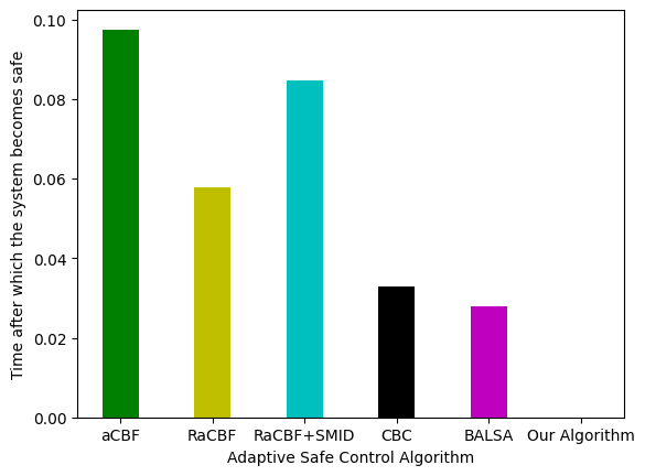
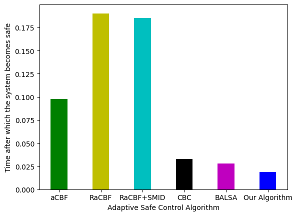
In this section, we demonstrate effectiveness of the proposed method using numerical simulations. The simulation code can be found with the supplementary materials. First, we tested algorithm 1 in an unknown one-dimensional linear dynamical system with unsafe (and unstable) nominal controller starting from a safe initial state near the boundary of the safe set $\mathcal{S}$. The performance is compared with Adaptive Safe Control Barrier function (aCBF) algorithm from [8]; Robust Adaptive Control Barrier Function (RaCBF) and RaCBF with Set Memebership Identification (RaCBF+SMID) (denoted here as RaCBFS) algorithms from [9]; the convex body chasing based algorithm $\mathcal{A}_{\pi}-$SEL algorithm from [17] (denoted here as cbc); and the Bayesian Learning based Adaptive Control for Safety Critical Systems (BALSA) algorithm from [10] (denoted here as balsa). (See appendix XI-A for implementation details.) Algorithm 1 acted safely at all times when the state originated from a point within the safe region (forward invariance), even before other algorithms could obtain sufficient information (samples) to exhibit safe behaviors (Figure 1(a)). This demonstrates the safety merit 1 of our proposed algorithm 1. When the same algorithms were started from an unsafe state outside the safe set $\mathcal{S}$, we observe a quick recovery (Figure 1(b)). This demonstrates the recovery merit 2 of our proposed algorithm 1.

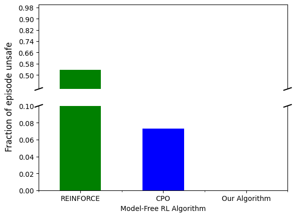
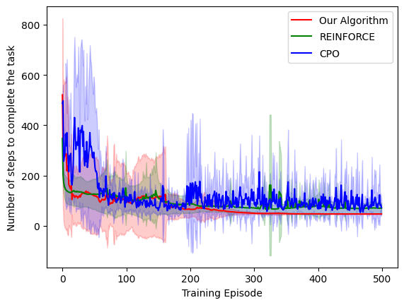
Next, we tested algorithm 2 for a non-linear four-dimensional extension of the vehicular yaw dynamics system (as described in Appendix XI-B) with continuous state and action spaces. We compared its performance and safety against some model-free reinforcement learning algorithms like REINFORCE from [45], and Constrained Policy Optimization (CPO) from [27]. The policy network in algorithm 2 predicted a random action, which was then clipped within reasonable limits to obtain $a_{n}$ at each instance $n$. (See appendix XI-B for implementation details.) We observe from figure 1(c), that the average fraction of time the system was unsafe during a training epoch improves as we go from the naive REINFORCE algorithm, to the CPO algorithm but it fails to achieve zero-violation safety, which is in contrast to our algorithm 2 that achieves zero-violation safety as well. Further from 1(d), we observe that the number of steps needed to accomplish the task (after convergence) and the convergence rate of our algorithm 2 is comparable with the other two algorithms, thus showing that algorithm 2 does not suffer any compromise in its performance or convergence rate. Our tool therefore enables the REINFORCE like algorithm to learn a safe policy via a completely safe exploration process. This demonstrates the applicability to RL merit 3 of our technique.

(a)

(b)

(c)

(d)

Figure 1: Comparing (a) forward invariance and (b) forward convergence of our algorithm 1 with several safe adaptive control algorithms. (c) Comparing (c) safety rate and (d) convergence rate of algorithm 2 with other model-free RL algorithms.

VI Conclusion and Future Work

We proposed a sample-optimal technique that ensures zero-violation safety at all times for systems with large uncertainties in the system dynamics and demonstrated its applicability to safe exploration in reinforcement learning problems. Possible future works include extensions to discrete-time systems; non-deterministic systems with an additive noise; integration into other reinforcement learning algorithms such as [46, 47, 48].

APPENDIX

VII Proof of Theorem III.2

We have a few preliminary lemmas, before starting the proof of theorem III.2. We begin with the following lemma which is a extension of the well-known Nagumo’s theorem [1] to the settings when the dynamics $x_{t}$ does not need to be differentiable w.r.t. $t$, but only requires the existence of left and right hand derivatives w.r.t. $t$, and we present an independent elementary proof of the lemma below.

Lemma VII.1.

Let $h\mathrel{\mathop{\mathchar 58\relax}}\mathbb{R}^{d}\rightarrow\mathbb{R}$ be a differetiable function, and let $x_{t}\mathrel{\mathop{\mathchar 58\relax}}\mathbb{R}_{\geq 0}\rightarrow\mathbb{R}^{d}$ denote the state-variable of a dynamical system which is continuous with respect to time $t$ and such that $\dot{x}^{+}_{t}$ exists $\forall t$. Let $\mathcal{C}\triangleq\left\{x\mathrel{\mathop{\mathchar 58\relax}}h(x)\geq 0\right\},$ and let $\partial\mathcal{C}\triangleq\left\{x\mathrel{\mathop{\mathchar 58\relax}}h(x)=0\right\}$ be the boundary of the set $\mathcal{C}$, $int(\mathcal{C})\triangleq\mathcal{C}\setminus\partial\mathcal{C}$ be the interior of $\mathcal{C}$, and let $T>0$ be any finite time-horizon. If the following conditions hold:

S-1: $x_{0}\in int(\mathcal{C})$.

S-2: $x_{t}\notin int(\mathcal{C})\implies\dot{h}^{+}(x_{t})>0$.

Then

$$x_{t}\in\mathcal{C},~{}~{}\forall t\in[0,T].$$ (24)

We need a couple of lemmas to prove lemma VII.1. We begin with the following lemma which is a straightforward extension of the chain rule for differentiation to right hand derivatives.

Lemma VII.2.

If $\phi\mathrel{\mathop{\mathchar 58\relax}}\mathbb{R}^{d}\rightarrow\mathbb{R}$ is differentiable with respect to $x$, $\forall x\in\mathbb{R}^{d}$, if $x_{t}$ is continuous with respect to time $t$ such that $\dot{x}^{+}_{t}$ exists at all times $t$, then

$$\dot{\phi}^{+}(x_{t})=\nabla\phi(x_{t})\cdot\dot{x}^{+}_{t}.$$ (25)

Proof (Lemma VII.2).

Since $\phi(x)$ is differentiable with respect to $x$, we define $Q(y,x_{t})$ for any $y\in\mathbb{R}^{d}$ as:

$$Q(y,x_{t})=\begin{cases}\begin{pmatrix}\frac{\phi(y)_{1}-\phi(x_{t})_{1}}{y_{1}-{x_{t}}_{1}}\\ \vdots\\ \frac{\phi(y)_{i}-\phi(x_{t})_{i}}{y_{i}-{x_{t}}_{i}}\\ \vdots\\ \frac{\phi(y)_{d}-\phi(x_{t})_{d}}{y_{d}-{x_{t}}_{d}}\\ \end{pmatrix}\text{ if }y\neq x_{t},\\ \nabla\phi(x_{t})\text{ otherwise.}\end{cases}$$

We observe that $Q(y,x_{t})$ is continuous with respect to $y$ due to the differentiability of $\phi$ at $x_{t}$. And since $x_{\tau}$ is continuous with respect to $\tau$, so $Q(x_{\tau},x_{t})$ is also continuous with respect to $\tau$. Now let $\tau=t+\delta t$, for some $\delta t>0$. Then, we have:

$$\dot{\phi}^{+}(x_{t}) =\lim_{\delta t\rightarrow 0^{+}}\frac{\phi(x_{t+\delta t})-\phi(x_{t})}{\delta t}$$

$$=\lim_{\tau\rightarrow t^{+}}Q(x_{\tau},x_{t})\cdot\frac{1}{\tau-t}(x_{\tau}-x_{t})$$

$$=\lim_{\tau\rightarrow t^{+}}Q(x_{\tau},x_{t})\cdot\lim_{\tau\rightarrow t^{+}}\frac{1}{\tau-t}(x_{\tau}-x_{t})$$

$$=Q(x_{t},x_{t})\cdot\dot{x}^{+}_{t}$$

$$=\nabla\phi(x_{t})\cdot\dot{x}^{+}_{t},$$

where the first line uses the definition of right hand derivatives, the second line follows from the definition of $Q(x_{\tau},x_{t})$, the third and fourth line use the continuity of $Q(x_{\tau},x_{t})$ with respect to $\tau$, the existence of $\dot{x}^{+}_{t}$, and the fact that the limit of a product of two functions is the product of the limits of the two functions when the limits exist, and the last line again follows from the definition of $Q(y,x_{t})$. ∎

Similarly, we can also prove the following:

Lemma VII.3.

If $\phi\mathrel{\mathop{\mathchar 58\relax}}\mathbb{R}^{d}\rightarrow\mathbb{R}$ is differentiable with respect to $x,\forall x\in\mathbb{R}^{d}$, if $x_{t}$ is continuous with respect to time $t$ such that $\dot{x}^{-}_{t}$ exists at all times $t$, then

$$\dot{\phi}^{-}(x_{t})=\nabla\phi(x_{t})\cdot\dot{x}^{-}_{t}.$$ (26)

The next lemma is another result required in the proof of lemma VII.1. It resembles a direct consequence of the Lagrange’s mean value theorem for differentiable functions if the function were differentiable.

Lemma VII.4.

Let $h(t)$ be a continuous function of $t$ with its right-hand derivative $\dot{h}^{+}$ defined for every $t$. Let $t_{1}<t_{2}$ be such that $h(t_{1})>h(t_{2})$, then there exists a $t_{3}\in(t_{1},t_{2})$ such that $\dot{h}^{+}(t_{3})\leq 0$.

Proof.

For contradiction, assume

$$\dot{h}^{+}(\tau)>0,~{}~{}\forall\tau\in(t_{1},t_{2}).$$ (27)

We partition the interval $[t_{1},t_{2}]$ into $k$ equal intervals: $[t_{i,1},t_{i,2}]$ for $i=1,2,\ldots,k$, such that $t_{1,1}=t_{1}$, $t_{k,2}=t_{2}$, and $t_{i+1,1}=t_{i,2}$, and $t_{i,1}+t_{i+1,2}=2t_{i,2}$, $\forall i\in\{1,2,\ldots,k-1\}$. Thus, we have

$$[t_{1},t_{2}]=\bigcup_{i=1}^{k}[t_{i,1},t_{i,2}],~{}~{}\text{where }[t_{i,1},t_{i,2}]\cap[t_{j,1},t_{j,2}]=\emptyset~{}~{}\forall i\neq j.$$

Since $h(t_{1})>h(t_{2})$, there exists $i\in\{1,2,\ldots,k\}$ such that $h(t_{i,1})>h(t_{i,2})$, otherwise $h(t_{1})=h(t_{1,1})\leq h(t_{1,2})=h(t_{2,1})\leq h(t_{2,2})=\ldots=h(t_{k,2})=h(t_{2})$, a contradiction. For this $i$, we define $f_{1}=\dot{h}^{+}(t_{i,1})$. By our contrary assumption (27), $f_{1}>0$. Next we partition this interval $[t_{i,1},t_{i,2}]$ again into $k$ equal parts exactly as above (note that we again have $h(t_{i,1})>h(t_{i,2})$) to get the number $f_{2}$. We keep repeating the process to generate the sequence: $f_{1},f_{2},\dots$. We observe that each number $f_{j}$ in the above sequence is positive as argued above, and since the function $h(t)$ is right-differentiable everywhere in $(t_{1},t_{2})$ and the sequence is constructed by sub-partitioning the previous partition within $[t_{1},t_{2}]$, the sequence $\{f_{l}\}_{l=1}^{\infty}$ converges to $\dot{h}^{+}(t_{3})$ for some $t_{3}\in(t_{1},t_{2})$. Further, since each $f_{l}$ is generated from a partition interval $[t_{i(l)},t_{j(l)}]$, such that $h(t_{i(l)})>h(t_{j(l)})$, and the function $h$ is right hand differentiable, we must have $\lim_{l\rightarrow\infty}f_{l}\leq 0$. So, we have

$$\dot{h}^{+}(t_{3})=\lim_{l\rightarrow\infty}f_{l}\leq 0,$$ (28)

which contradicts (27) since $t_{3}\in(t_{1},t_{2})$. Thus, we have the desired lemma. ∎

We are now ready to prove lemma VII.1.

Proof (Lemma VII.1).

Since $h(x)$ is differentiable with respect to $x$ and $x_{t}$ is continuous in $t$, $h(x_{t})$ is continuous with respect to $t$. Since $\dot{x}_{t}^{+}$ is given by (1), then from lemma VII.2, we have: $\dot{h}^{+}(x_{t})=\nabla h(x_{t})\cdot\dot{x}_{t}^{+}$ exists for every $t\in[0,T]$.

Assume for contradiction, that

$$\exists\tau\in[0,T]~{}~{}\text{such that }h(x_{\tau})<0.$$ (29)

Now from S-1, we have $h(x_{0})>0$. So, we have $h(x_{0})>0>h(x_{\tau})$. Since $h(x_{t})$ is continuous in $t$, by the intermediate value theorem, there exists a $t^{*}\in(0,\tau)$ such that $h(x_{t^{*}})=0$ and $h(x_{t^{\prime}})<0$ for every $t^{\prime}\in(t^{*},\tau).$ So, we have $x_{t^{\prime}}\notin int(\mathcal{C})$ for every $t^{\prime}\in[t^{*},\tau]$. Now S-2 implies,

$$\dot{h}^{+}(x_{t})>0,~{}~{}\forall(t^{*},\tau).$$ (30)

Now setting $t_{1}=t^{*}$, $t_{2}=\tau$, in lemma VII.4 and since $h(x_{t^{*}})=0>h(x_{\tau})$, we have from lemma VII.4, that there exists $\tau^{\prime}\in(t^{*},\tau)$ such that:

$$\dot{h}^{+}(x_{\tau^{\prime}})\leq 0,$$ (31)

which contradicts (30). Thus, we have the desired lemma. ∎

Next we have the following lemmas regarding the properties of algorithm 1.

Lemma VII.5.

When algorithm 1 is used for dynamical system (1), we have:

$$\dot{x}^{-}_{t}=f(x_{t})+g(x_{t})u_{last}$$ (32)

Proof (Lemma VII.5).

Since $u_{t}$ in (1) has left hand limits, we have $\lim_{\tau\rightarrow t^{-}}u_{\tau}=u_{last}$. Further, since $u_{t}$ can have only finitely many jumps in any finite interval, and let $\delta t>0$ be sufficiently small such that $u_{t}$ is continuous in $[t-\delta t,t]$. Then, we have for any $\tau\in[t-\delta t,t]$ using (1), $x_{\tau}=x_{t-\delta t}+\int_{t-\delta t}^{\tau}\left(f(x_{s})+g(x_{s})u_{s}\right)ds$. Now using continuity of $f(x_{t})$, $g(x_{t})$, and $x_{t}$ with respect to $t$:

$$\dot{x}^{-}_{t} =\lim_{\delta t\rightarrow 0^{+}}\frac{x_{t}-x_{t-\delta t}}{\delta t}$$

$$=\lim_{\delta t\rightarrow 0^{+}}\frac{\int_{t-\delta t}^{t}\left(f(x_{s})+g(x_{s})u_{s}\right)}{\delta t}$$

$$=f(x_{t})+g(x_{t})\lim_{s\rightarrow t^{-}}u_{s}$$

$$=f(x_{t})+g(x_{t})u_{last}.$$

∎

Lemma VII.6.

Let algorithm 1 be used for the dynamical system (1), with a nominal controller $u_{nom}$ which is finite at any time $t$. Then the control action $u_{t}$ played by algorithm 1 is always finite at any finite time $t$.

Proof (Lemma VII.6).

From (1), we have a unique solution $x_{t}$ which is continuous in time $t$. So, the state variable $x_{t}$ is finite at any finite time $t$. Now at any point $t$, the control action $u_{t}$ applied by algorithm 1 is either the finite control action $u_{nom}$ provided by the nominal controller or the correction control action $u_{corr}$ given by (18). Now using an inductive argument, if $u_{\tau}$ is finite for all $\tau<t$ (vacuously true for $t=0$), then $u_{last}$ is finite. Further, from continuity of $f$ and $g$, and (32) from lemma VII.5, we have a finite $\dot{x}^{-}_{t}$ at any finite time $t$. Further, by (17) and assumption 2, $\hat{g}^{+}(x_{t})$ is also finite at any finite time $t$. From (15), we also observe that $\Gamma_{t}$ can be chosen as a matrix with finite entries at any finite time $t$. Thus, by equation (18), $u_{corr}$ is finite at any finite time $t$. Thus, in both cases the control action $u_{t}$ applied by algorithm 1 is finite for any finite time $t$. ∎

Lemma VII.7.

When algorithm 1 is used for dynamical system (1), the following holds for any time $t$:

$$\phi(x_{t})\leq\theta\implies\dot{\phi}^{+}(x_{t})\geq\eta>0.$$

Proof (Lemma VII.7).

Let $t$ be such that $\phi(x_{t})\leq\theta$. Then algorithm 1 plays $u=u_{corr}$ given by (18). So, we have:

$$\dot{\phi}^{+}(x_{t}) =\nabla\phi(x_{t})\cdot\dot{x}_{t}^{+}$$ (33)

$$=\nabla\phi(x_{t})\cdot\left(f(x_{t})+g(x_{t})u_{corr}\right)$$ (34)

$$=\nabla\phi(x_{t})\cdot\left(f(x_{t})+g(x_{t})u_{last}-g(x_{t})\hat{g}^{+}(x_{t})\Gamma_{t}\dot{x}_{t}^{-}\right)$$ (35)

$$=\nabla\phi(x_{t})\cdot\left(\dot{x}_{t}^{-}-g(x_{t})\hat{g}^{+}(x_{t})\Gamma_{t}\dot{x}_{t}^{-}\right)$$ (36)

$$=\dot{\phi}^{-}(x_{t})-\nabla\phi(x_{t})\cdot\left(g(x_{t})\hat{g}^{+}(x_{t})\Gamma_{t}\dot{x}_{t}^{-}\right)$$ (37)

where (33) uses (25), (34) uses (1), (35) uses (18), (36) uses (32), and (37) uses (26). Now let

$$y_{t}=\Gamma_{t}\dot{x}_{t}^{-}.$$ (38)

Then, from (2), (3), (16) and (17), we have:

$$g(x_{t})\hat{g}^{+}(x_{t})y_{t}=\sum_{i=1}^{k_{t}}\frac{\lambda_{i,t}}{\hat{\lambda}_{i,t}}\langle U_{i,t},y_{t}\rangle U_{i,t}.$$ (39)

Now using (38), and (12) in (39), and the orthonormality of the $U_{i,t}$ vectors we have:

$$\nabla\phi(x_{t})\cdot\left(g(x_{t})\hat{g}^{+}(x_{t})\Gamma_{t}\dot{x}_{t}^{-}\right)=\sum_{i=1}^{k_{t}}\beta_{i,t}\frac{\lambda_{i,t}}{\hat{\lambda}_{i,t}}\langle U_{i,t},y_{t}\rangle.$$ (40)

Now, we define $\epsilon_{i,t}$, for every $i\in\{1,\ldots,k_{t}\}$ as:

$$\epsilon_{i,t}\triangleq\alpha_{t}\beta_{i,t}-\frac{\lambda_{i,t}}{\hat{\lambda}_{i,t}}\langle U_{i,t},y_{t}\rangle.$$ (41)

So we have,

$$\dot{\phi}^{+}(x_{t}) =\dot{\phi}^{-}(x_{t})-\nabla\phi(x_{t})\cdot\left(g(x_{t})\hat{g}^{+}(x_{t})\Gamma_{t}\dot{x}_{t}^{-}\right)$$

$$=\dot{\phi}^{-}(x_{t})-\sum_{i=1}^{k_{t}}\beta_{i,t}\left(\alpha_{t}\beta_{i,t}-\epsilon_{i,t}\right)$$ (42)

$$=\dot{\phi}^{-}(x_{t})-\alpha_{t}\sum_{i=1}^{k_{t}}\beta_{i,t}^{2}+\sum_{i=1}^{d}\beta_{i,t}\epsilon_{i,t}$$ (43)

$$=\dot{\phi}^{-}(x_{t})-\langle\nabla\phi(x_{t}),\dot{x}_{t}^{-}\rangle+\eta+\sum_{i=1}^{k_{t}}\beta_{i,t}\epsilon_{i,t}$$ (44)

$$=\eta+\sum_{i=1}^{k_{t}}\beta_{i,t}\epsilon_{i,t},$$ (45)

where we get (42) from substituting (40),(41) in (37), we get (44) using (13), (14) and the fact that $u_{i,t}$’s are orthonormal and $k_{t}=d$, which implies

$$\langle\nabla\phi(x_{t}),\dot{x}^{-}_{t}\rangle-\eta=\alpha_{t}\mathinner{\!\left\lVert\nabla\phi(x_{t})\right\rVert}^{2}=\alpha_{t}\sum_{i=1}^{d}\beta_{i,t}^{2}=\alpha_{t}\sum_{i=1}^{k_{t}}\beta_{i,t}^{2},$$

and we get (45) using (26).

Now, in order to prove $\dot{\phi}^{+}(x_{t})\geq\eta>0$, it suffices to show that:

$$\sum_{i=1}^{k_{t}}\beta_{i,t}\epsilon_{i,t}\geq 0.$$ (46)

Substituting for $\epsilon_{i,t}$ from (41) and $y_{t}$ from (38) in the above constraint (46), we get the following constraint on the matrix $\Gamma_{t}$:

$$\sum_{i=1}^{k_{t}}\beta_{i,t}\left(\alpha_{t}\beta_{i,t}-\frac{\lambda_{i,t}}{\hat{\lambda}_{i,t}}U_{i,t}^{\intercal}\Gamma_{t}\dot{x}_{t}^{-}\right)\geq 0.$$ (47)

Now, using the bounds on the estimates of the singular values of $g(x_{t})$ from (4), we observe that any solution $\Gamma_{t}$ to the set of $d$ inequalities in (15) would make each of the $d$ terms in (47) non-negative. Thus, our algorithm’s choice of $\Gamma_{t}$ satisfies the overall constraint (47), thereby implying $\dot{\phi}(x_{t})^{+}\geq\eta$ (from (45) and (46)), and proving the claim. ∎

We are now ready to prove the main result of this section, theorem III.2, using lemma VII.1, lemma VII.2 and lemma VII.7.

Proof (Theorem III.2).

We set $h(x_{t})=\phi(x_{t})-\theta$, $\mathcal{C}=\mathcal{S}_{\theta}$ in lemma VII.1. In case of forward invariance, we have $x_{0}\in\mathcal{S}_{\theta}$. This makes condition S-1 of lemma VII.1 true for our choice of $h$ and $\mathcal{C}$. Since $\phi(x)$ is differentiable with respect to $x$ and $x_{t}$ is continuous in time $t$, $\phi(x_{t})$ is continuous in $t$. Thus, we have $h$ satisfying the conditions of lemma VII.1. Further, from lemma VII.6, $u_{t}$ applied by algorithm 1 is finite. Then by equation (1) we conclude that $\dot{x}_{t}^{+}$ always exists. Thus, lemma VII.1 is applicable for our choice of $h$ and $\mathcal{C}$ and lemma VII.7 guarantees that S-2 of lemma VII.1 holds true as well. Thus, by lemma VII.1 the set $\mathcal{S}_{\theta}$ is forward invariant as desired.

Now using lemma VII.7, the forward convergence of $\mathcal{S}_{\theta}$ (part $2$ of theorem III.2) can also be guaranteed. In particular, we show a forward convergence rate for $\mathcal{S}_{\theta}$ as follows. Let

$$d(x_{t},\mathcal{S}_{\theta})=\theta-\phi(x_{t})>0.$$ (48)

Since $x_{0}\notin\mathcal{S}_{\theta}$, from lemma VII.7 we have $\dot{\phi}^{+}(x_{t})\geq\eta$ whenever $\phi(x_{t})<\theta$. This uniform lower bound on $\dot{\phi}^{+}$ implies (using mean value theorem on $\phi$), that within time:

$$\tau\leq\frac{d(x_{t},\mathcal{S}_{\theta})}{\eta},$$ (49)

the system reaches the safety region $\mathcal{S}_{\theta}$. Also, for a finite $x_{t}$ by lemma VII.6, the control action played by algorithm 1: $u_{t}$ is bounded. So, by equation (1), within finite duration $\tau$, the state variable $x_{t}$ remains bounded throughout. So, by using lemma VII.6 in an inductive way, we observe that the state variable $x_{t}$ as well as the applied control action $u_{t}$ always stays finite (bounded) in the case of forward convergence as well. We thus conclude the proof of theorem III.2. ∎

VIII Proof of Theorem III.1

Proof (Theorem III.1).

At time $t=0$, let $x_{0}\in\partial\mathcal{S}$, such that $\nabla\phi(x_{0})\neq 0$. From the assumption in theorem III.1, we know such a state $x_{0}\in\partial\mathcal{S}$ exists. For the above choice of $x_{0}$, we have $I(0,0)=\{x_{0}\}$ at $t=0$. Then, we show that any controller observing just the sample $x_{0}$ cannot guarantee the forward invariance of $\mathcal{S}$. Let the controller play $u_{0}$ at time $t=0$. Choose any $f(.)$ which satisfies $f(x_{0})=-\nabla\phi(x_{0})-g(x_{0})u_{0}$. We the have:

$$\dot{\phi}^{+}(x_{0})=\nabla\phi(x_{0})\cdot(f(x_{0})+g(x_{0})u_{0})=-\mathinner{\!\left\lVert\nabla\phi(x_{0})\right\rVert}^{2}<0,$$

where the first equality uses (1), lemma VII.2, and the above choice of $f(.)$, and the inequality follows since $\nabla\phi(x_{0})\neq 0$ for our choice of $x_{0}$. Further, since $x_{0}\in\partial\mathcal{S}$, $\dot{\phi}(x_{0})<0$ implies there exists an $\epsilon$ such that for any $\tau\in(0,\epsilon)$, $\phi(x_{\tau})<0$, i.e. $x_{\tau}\notin\mathcal{S}$ and thus the algorithm fails to guarantee forward invariance of $\mathcal{S}$ in this interval. Since the function $f(.)$ is unknown to the controller, our choice of the $f(.)$ above is valid, and we can construct such $f$ for every controller $u$. We have thus shown the existence of a system corresponding to that particular controller whose dynamics equation is of the form (1), where the controller fails to guarantee the forward invariance of $\mathcal{S}$ with respect to the system. This proves theorem III.1.

∎

IX Proof of Theorem IV.1

Proof (Theorem IV.1).

Let $\mathcal{H}$ be the set of possible state action trajectories indexed by $e$. Let $\ell_{e}\in\mathcal{H}$ denote the state action trajectory observed in the roll-out for episode $e$,

$$\ell_{e}=\{s_{n},a_{n},u_{n}\}_{n=0}^{\infty},$$ (50)

and let

$$R(\ell_{e})=\sum_{n=0}^{\infty}\gamma^{n}r(s_{n},u_{n})$$ (51)

denote the discounted sum reward for trajectory $\ell_{e}=\{s_{n},a_{n},u_{n}\}_{n=0}^{\infty}\in\mathcal{H}$.

Let $P_{w}$ denote the probability density function of trajectories induced by the correction controller (18) and the current stochastic policy $\pi_{w}$. By construction, for any trajectory $\ell_{e}=\{s_{0},a_{0},u_{0},s_{1},a_{1},u_{1},\ldots\}$, $P_{w}(\ell_{e})$ given by

$$P_{w}(\ell_{e}) =\pi_{w}(a_{0}|s_{0})\Pr[u_{0}=C(s_{0},\dot{s}_{0}^{-},a_{0},u_{-1})]\Pr[s_{1}|s_{0},u_{0}]$$

$$\pi_{w}(a_{1}|s_{1})\Pr[u_{1}=C(s_{1},\dot{s}_{1}^{-},a_{1},u_{0})]\Pr[s_{2}|s_{1},u_{1}]\ldots,$$ (52)

is the induced probability density function supported on the set of possible trajectories $\mathcal{H}$. Further, since $C(s_{n},\dot{s}_{n}^{-},a_{n},u_{n-1})$ is a deterministic function given by (18), so we have $\Pr[u_{n}=C(s_{n},\dot{s}_{n}^{-},a_{n},u_{n-1})]=1,~{}\forall n$ in the above. Therefore, we can write:

$$\nabla_{w}J(w)=\nabla_{w}\operatorname{\mathbb{E}}_{\ell_{e}\sim P_{w}}R(\ell_{e})$$

$$=\nabla_{w}\int_{\ell_{e}\in\mathcal{H}}R(\ell_{e})P_{w}(\ell_{e})d\ell_{e}$$

$$=\int_{\ell_{e}\in\mathcal{H}}R(\ell_{e})\nabla_{w}P_{w}(\ell_{e})d\ell_{e}$$

$$=\int_{\ell_{e}\in\mathcal{H}}P_{w}\left(\ell_{e}\right)\left(\frac{\nabla_{w}P_{w}(\ell_{e})}{P_{w}(\ell_{e})}R(\ell_{e})\right)d\ell_{e}$$

$$=\operatorname{\mathbb{E}}_{\ell_{e}\sim P_{w}}\nabla_{w}\ln P_{w}(\ell_{e})R(\ell_{e})$$

$$=\operatorname{\mathbb{E}}_{\ell_{e}\sim P_{w}}R(\ell_{e})\nabla_{w}\{\ln\pi_{w}(a_{0}|s_{0})$$

$$+\ln\Pr[u_{0}=C(s_{0},\dot{s}^{-}_{0},a_{0},u_{-1})]+\ln\Pr[s_{1}|s_{0},u_{0}]$$

$$+\ln\pi_{w}(a_{1}|s_{1})+\ldots\}$$

$$=\operatorname{\mathbb{E}}_{\ell_{e}\sim P_{w}}\sum_{n=0}^{\infty}\left[\nabla_{w}\ln\pi_{w}(a_{n}|s_{n})\right]R(\ell_{e})$$

$$=\operatorname{\mathbb{E}}_{\ell_{e}\sim P_{w}}\widehat{\nabla J(w)}.$$ (53)

Here, in the second line we exchanged the integral with the gradient using the Leibniz integral rule, and the second to last line uses the fact that $\Pr[s_{n}|s_{n-1},u_{n}],~{}C(s_{n},\dot{s}_{n}^{-},a_{n},u_{n-1})$ are independent of the policy parameters $w$. In particular, $\ln\Pr[C(s_{n},\dot{s}_{n}^{-},a_{n},u_{n-1})]=0,~{}\forall n$, and is independent of $w$. So, the gradient of these log probabilities with respect to $w$ is zero. From (IX), we see that the gradient estimate $\widehat{\nabla J(w)}$ used by algorithm 2 is indeed an unbiased estimate of the true policy gradient $\nabla_{w}J(w)$. ∎

X Bicycle dynamics example illustrating the applicability of assumptions 1 and 2

In this section, we show an example of bicycle dynamics where our assumptions 1 and 2 are applicable to a reasonable partial model of the dynamics.
We consider a special case of our assumed setting where the matrix $g(x_{t})$ always admits an SVD with known constant matrices $U_{t}=U$ and $V_{t}=V$, and when some gross upper and lower bounds on the singular values are available. For example, in vehicular yaw dynamics of a bicycle, if we only have the knowledge of axis lengths, mass and moment of inertia about the vertical axis ( quantities easier to measure ), then it is sufficient to apply our proposed method since the setting falls under our assumptions 1 and 2 as demonstrated below. The two-dimensional yaw dynamics of a bicycle is typically modeled with state $x_{t}=\left[v(t)~{}r(t)\right]^{\intercal}$ as:

$$\begin{bmatrix}\dot{v}(t)\\ \dot{r}(t)\end{bmatrix}=\begin{bmatrix}-\frac{c_{r}+c_{f}}{mu}&\frac{c_{r}a_{2}-c_{f}a_{1}}{mu}-u\\ \frac{c_{r}a_{2}-c_{f}a_{1}}{uI_{z}}&-\frac{c_{f}a_{1}^{2}+c_{r}a_{2}^{2}}{uI_{z}}\end{bmatrix}\begin{bmatrix}v(t)\\ r(t)\end{bmatrix}+\begin{bmatrix}\frac{c_{f}}{m}\\ \frac{c_{f}a_{1}}{I_{z}}\end{bmatrix}\delta_{f},$$ (54)

where $m$ is the vehicle mass; $a_{1},a_{2}$ are the distances to the center of mass point of the front and rear wheels respectively; $I_{z}$ is the vehicle’s moment of inertia about the $z$-axis (the bicycle moves in the $x$-$y$ plane); $r$ is the angular velocity (anti-clockwise) of the turn being made by the bicycle steering; $u$ is the bicycle’s velocity along the $x$-axis (direction of its initial motion); $v$ is the velocity along $y$-axis (direction along which it is turning); $c_{f},c_{r}$ are the unknown cornering stiffness constants of the front and rear wheels; and $\delta_{f}$ is the only control action which is the angle of left turn applied through the handle ([49]). Here, the matrix $g(.)$ is constant and admits the following singular value decomposition:

$$\begin{bmatrix}\frac{c_{f}}{m}\\ \frac{c_{f}a_{1}}{I_{z}}\end{bmatrix}=\begin{bmatrix}\frac{\lambda_{1}}{\lambda}&\frac{\lambda_{2}}{\lambda}\\ \frac{\lambda_{2}}{\lambda}&-\frac{\lambda_{1}}{\lambda}\end{bmatrix}\begin{bmatrix}\lambda\\ 0\end{bmatrix}\begin{bmatrix}1\end{bmatrix},$$ (55)

where $\lambda=\sqrt{(c_{f}/m)^{2}+(c_{f}a_{1}/I_{z})^{2}}$ is the singular value $\lambda_{1}=\frac{c_{f}}{m}$, and $\lambda_{2}=\frac{c_{f}a_{1}}{I_{z}}$. Now if the stiffness parameters $c_{f},c_{r}$ are unknown (difficult to measure in a realistic setting), then $\lambda_{1}$, $\lambda_{2}$ would be unknown scalars, but the stiffness parameters would get cancelled out in the the normalized fractions $\frac{\lambda_{1}}{\lambda}$ and $\frac{\lambda_{2}}{\lambda}$ so these fractions would still be known to the user. Also, since $\lambda$ is strictly positive, any rough estimates on the unknown stiffness parameters would allow the user to guess a $\hat{\lambda}$ with $0<m\hat{\lambda}<\lambda<M\hat{\lambda}$, where $m$ and $M$ are known (ratio) bounds. Thus, such a system satisfies our assumptions 1 and 2.

XI Implementation Details of Numerical Simulations from section V

XI-A Comparison with Adaptive Safe Control Algorithms

We consider the simple one dimensional system below:

$$\dot{x}=1.5x+u,$$ (56)

where $f(x)=1.5x$, $g(x)=1$, with a nominal controller: $u_{nom}(x)=-x$. We define the safe set as $\mathcal{S}=[-0.2,0.2]$, and the initial state is $x_{0}=0.1999$. We use the same shorthand for denoting each algorithm as listed in the main paper section V.

1. [Algorithm 1] Here, for our algorithm we use the nominal controller $u_{nom}=-x$, which makes the closed loop dynamics:

   $$\dot{x}=0.5x,$$

   which is exponentially increasing with time and is expected to quickly exit the safe set $\mathcal{S}$. We choose the barrier function $\phi(x)=1-25x^{2}$, corresponding to our safe set $\mathcal{S}$ and we take $\theta=0.001$, and $\Gamma=4$.

2. [aCBF] For the Adaptive CBF algorithm [8], we have:
   $f(x)=x$, $g(x)=1$, $u_{nom}(x)=-x$, $F(x)=x$, $\theta^{*}=0.5$, $\Gamma=5$, $\hat{\theta}_{0}=0$, $\phi_{a}(x,\hat{\theta})=1-25x^{2}.$ This corresponds to the open loop dynamics 56.
   This gives us an adaptation rule of:

   $$\dot{\hat{\theta}} =\Gamma\tau(x,\hat{\theta}),$$ (57)

   $$\textrm{where }\tau(x,\hat{\theta}) =-F(x)\frac{\partial\phi_{a}}{\partial x}=50x^{2}.$$ (58)

   And for the $\lambda_{cbf}$ function we have:

   $$\lambda_{cbf}(x,\hat{\theta})=\hat{\theta}-\Gamma\frac{\partial\phi_{a}}{\partial\hat{\theta}}=\hat{\theta}.$$ (59)

   So, we have the $aCBF$ controller given by the following quadratic program:

   $$\text{minimize}_{u\in\mathbb{R}}~{}~{} \mathinner{\!\left\lVert u-u_{nom}(x)\right\rVert}$$

   subject to $$\sup_{u\in\mathbb{R}}(-50x[x+\hat{\theta}x+u])\geq 0.$$

3. [RaCBF] For the RaCBF algorithm [9], we have the same setting as above on the same system (56) and with the same $\lambda_{cbf}$ (59) and adaptation rule (57). But here, we assume that the error in parameter estimation: $\tilde{\theta}=\theta^{*}-\hat{\theta}\in[-\tilde{\nu},+\tilde{\nu}]$ (i.e. parameter estimation error lies in a bounded convex region). Here we have taken $\tilde{\nu}=2$. We also took $\alpha(x)$ as the identity function: $\alpha(x)=x$, so we have the following quadratic program for the RaCBF controller:

   $$\text{minimize}_{u\in\mathbb{R}}~{}~{} \mathinner{\!\left\lVert u-u_{nom}(x)\right\rVert}$$

   subject to $$\sup_{u\in\mathbb{R}}(-50x[x+\hat{\theta}x+u])$$

   $$\geq-\phi_{a}(x,\hat{\theta})+\frac{2}{5}.$$

4. [RaCBFS] This algorithm referred to as the RaCBF+SMID algorithm in [9] improves upon the previous algorithm (RaCBF) of the same paper, by updating the uncertainty bound $\tilde{\nu}$ periodically after every few instances. The algorithm, updates its uncertainty over $\theta^{*}$ so that it is consistent with the trajectory history so far. Depending on the hyperparameter $D$ (we have taken $D=0.07$), we set $r_{min}$ and $r_{max}$ such that at time $t$:

   $$\forall\theta\in[r_{min},r_{max}]\mathrel{\mathop{\mathchar 58\relax}}~{}~{}~{}~{}~{}~{}~{}~{}$$

   $$|\dot{x}_{\tau}-f(x_{\tau})-g(x_{\tau})u_{\tau}-F(x_{\tau})\theta| \leq D$$

   $$~{}~{}\forall\tau\in[0,t).~{}~{}~{}~{}~{}~{}~{}~{}~{}$$

   Now with this uncertainty quantification over $\theta^{*}$ given by $r_{min},r_{max}$, the algorithm updates $\tilde{\nu}$ every $2.5$ms (where the time horizon is 0.25s) as follows:

   $$\tilde{\nu}=\max\left\{|r_{min}-\hat{\theta}|,|r_{max}-\hat{\theta}|\right\}.$$

5. [cbc] This is the convex body chasing algorithm from [17]. Here we search for consistent models corresponding to a pair $(\alpha_{t},\beta_{t})$ at each round $t$ which serve as estimates for the actual parameters $(\alpha^{*},\beta^{*})$ governing the system dynamics as: $\dot{x}=\alpha^{*}x+\beta^{*}u$, with initial uncertainties taken as $|\alpha^{*}|\leq 5$, and $2.5\times 10^{-6}\leq\beta^{*}\leq 0.05$. Discretizing the system dynamics for a small sampling time $T_{s}=2.5\times 10^{-4}s$, we look for all candidates $(\alpha,\beta)$ consistent with the current trajectory history as the polytope $P_{t}\subset P_{t-1}$ given by the linear program corresponding to the constraints: $|\alpha x_{i}+\beta u_{i}-x_{i+1}|\leq\eta$, for all discrete points $i$ in history up to time $t$, where $\eta$ is a suitably chosen hyperparameter. At every discrete step $t$, then the candidate $(\alpha_{t},\beta_{t})\in P_{t}$ is chosen as the Euclidean projection of the previous candidate $(\alpha_{t-1},\beta_{t-1})$ on the current polytope: $P_{t}$. At every round $t$, once the candidate model parameters $(\alpha_{t},\beta_{t})$ are found the control action $u_{t}$ is then chosen as: $u_{t}=-\frac{\alpha_{t}}{\beta_{t}}x_{t}$. The loss function $\mathcal{G}(x_{t},u_{t})$ is taken as the indicator function, $\mathcal{G}(x_{t},u_{t})=\mathbf{1}\{x_{t}\notin\mathcal{S}\}.$

6. [balsa] This is the Bayesian learning for adaptive safety algorithm from [10]. Here a proxy $\hat{f}(x)$ for the function $f(x)$ is available to the controller and it has full knowledge of $g(x)$. From the pseudo control $\mu$, it computes the control action as:

   $$u =g^{-1}(x)(\mu-\hat{f}(x)),\text{ where }$$ (60)

   $$\mu =\mu_{rm}+\mu_{pd}+\mu_{qp}-\mu_{ad}.$$ (61)

   Here, the modelling error $\Delta(x)=f(x)-\hat{f}(x)$ is estimated by a Bayesian Neural Network estimator that takes as input $x$ and predicts $m,s$ as the mean and standard deviation of the prediction $\Delta(x)$. The neural network is trained on the trajectory data history after every $0.025s$, where the total horizon is $0.25s$. From this we sample $\mu_{ad}\sim\mathcal{N}(m,s^{2})$ for the adaptive part of the pseudo control to cancel the modelling error. For this setting, we have taken $\mu_{rm}=0$ (since there is no tracking here), $\mu_{pd}(x)=\dot{x}-g(x)u_{last}+g(x)u_{nom}(x)=\mu_{nominal}(x)$, which is the effective pseudo control for our nominal controller used in 1. Finally the pseudo control $\mu_{qp}$ for safety is obtained by solving the quadratic program:

   $$\text{minimize}_{\mu_{qp},d\in\mathbb{R}}~{}~{} \mu_{qp}^{2}+5d^{2}$$

   subject to: $$\phi_{0}+\phi_{1}\mu_{qp}\geq d$$

   $$d\leq 0,$$

   where $\phi_{0}=\nabla\phi(x)\cdot\mu_{pd}(x)$, and $\phi_{1}=\nabla\phi(x)$.

When $x_{0}=0.1999$, the forward invariance data was observed as shown by figure 1(a), and when $x_{0}=0.2500$, a forward convergence (recovery) was observed as shown by figure 1(b).

XI-B Comparison with RL Algorithms

We consider a 4-dimensional extension of the non-linear vehicular yaw dynamics (54) given by with state $x_{t}=[V_{y},r,\psi,y]^{\intercal}$ and the dynamics:

$$\dot{x}_{t}=\begin{bmatrix}\frac{-c_{0}}{mV}&\frac{-c_{1}}{mV}-V&0&0\\ \frac{-c_{1}}{I_{z}V}&\frac{-c_{2}}{I_{z}V}&0&0\\ 0&1&0&0\\ \cos\psi&0&V_{x}\frac{\sin\psi}{\psi}&0\end{bmatrix}\begin{bmatrix}V_{y}\\ r\\ \psi\\ y\end{bmatrix}+\begin{bmatrix}\frac{C_{\alpha f}}{m}\\ \frac{aC_{\alpha f}}{I_{z}}\\ 0\\ 0\end{bmatrix}\delta,$$ (62)

where $V_{y}$ is the velocity of the vehicle along the lateral direction to which it is pointing, $V_{x}$ is the velocity along the direction the vehicle is headed, $V=\sqrt{V_{x}^{2}+V_{y}^{2}}$ is the net magnitude of the vehicle’s velocity, $r=\dot{\psi}$, is the yaw-rate i.e., the clockwise angular velocity along which the vehicle is turning in the $x-y$ plane (horizontal plane, the vehicle intends to take a right turn facing north to facing east eventually), $\psi$ is the yaw i.e., the current heading angle (clockwise) it makes from North towards East directions, and $y$ is the lateral displacement of the vehicle from the starting position (ideally we don’t want the vehicle to move much and take a successful right turn without displacing too much). $m$ is the mass of the vehicle, $I_{z}$ is the moment of inertia of the angle along the vertical axis (direction of gravity) about which the vehicle rotates to take the turn, and $a$ is the distance between the center of the mass of the vehicle to front wheel. The control variable is the scalar variable $\delta$, which is the steering angle applied by the controller.

We assume all the state variables are completely observable, $C_{\alpha f},m$ are known and $a,I_{z}$ are known only upto an unknown scaling factor. The parameters $c_{0},c_{1},c_{2},$ depend on several drag and stiffness parameters which are harder to model/estimate. So, the first matrix (the product of the $4\times 4$ matrix with the state vector) is the $f(x)$ vector which can be completely unknown to the user, the second matrix ($4\times 1$ matrix) is the $g(x)$ matrix, where the SVD becomes:

$$[C_{\alpha f}/m,aC_{\alpha f}/I_{z},0,0]^{\intercal}=$$ (63)

$$\begin{bmatrix}\frac{1/m}{\sqrt{1/m^{2}+a^{2}/I_{z}^{2}}}&\frac{-a/I_{z}}{\sqrt{1/m^{2}+a^{2}/I_{z}^{2}}}&0&0\\ \frac{a/I_{z}}{\sqrt{1/m^{2}+a^{2}/I_{z}^{2}}}&\frac{1/m}{\sqrt{1/m^{2}+a^{2}/I_{z}^{2}}}&0&0\\ 0&0&1&0\\ 0&0&0&1\end{bmatrix}\begin{bmatrix}\lambda\\ 0\\ 0\\ 0\end{bmatrix}\begin{bmatrix}C_{\alpha f}\end{bmatrix}^{\intercal},$$ (64)

where $\lambda=\sqrt{\frac{1}{m^{2}}+\frac{a^{2}}{I_{z}^{2}}}$. In the above SVD, the matrices $U$, $V$ are completely known since $m$, $C_{\alpha f}$ are known and the ratio $a/I_{z}$ is also known. Further, the singular value $\lambda$ is also known for this example. In order to demonstrate the effectiveness of our method, in our simulation we only used an estimate of the singular value $\lambda$ within known factors of $0.2$ and $5$. In particular, we took: $m=100,~{}I_{z}=20,~{}a=1,~{}m=0.2,~{}M=5,~{}C_{\alpha f}=10$. For the simulation, we took $c_{0}=70$, $c_{1}=40$, $c_{2}=180$, and an initial net velocity $V=5$. All the state variables were initialized at zero, and since the applied control may increase the velocity and yaw rates, they were clipped between $\pm 7$ and $\pm 350$ units respectively while running the dynamics, so as to keep all quantities within a realistic range. Further, the control variable applied according to the nominal controller (policy network) (7), or the applied correction control (18) was always clipped within $\pm 100$ to stay within realistic controller limitations (such bounds are not within assumptions 2 and 1, but our algorithm still works for this simulation).

For the reinforcement learning algorithms, we have used a policy network with just two hidden layers of $100$ neurons each, the input layer takes the $4$-dimensional state variable as input and the output layer predicted the mean value of the control action. The action chosen by the reinforcement learning algorithm was a Gaussian random variable as predicted by the policy network and standard deviation $0.7$. The discretization interval was $T_{s}=0.02$. All the three algorithms were trained for $500$ episodes and each episode consisted of an integer number of steps until it succeeded to achieve the right turn within a maximum of $1000$ steps (if the agent failed to achieve the goal within $1000$ steps it failed that episode). All the simulations were done for a set of $10$ experiments and the averaged data within $pm$ standard deviation are plotted in figures 1(d) as the convergence rate plot. The averaged data over these experiments regarding the safety fraction (or percentage) is plotted in figure 1(c).

The reward was set as

$$r(s_{n},a_{n},s_{n+1})=$$

$$\begin{cases}-4+\frac{1}{4}(\frac{1}{(\psi_{n}-\pi/2)^{2}+0.0001})\text{ if }|\psi_{n+1}-\pi/2|>\pi/36\\ 7000\text{ if }|\psi_{n+1}-\pi/2|<\pi/36\text{ and terminate if this occurs. }\end{cases}$$ (65)

Similarly, the cost (penalizing unsafe behavior) for the CPO algorithm benchmark was defined as:

$$c(s_{n},a_{n},s_{n+1})=$$

$$\min\{(0.004(r_{n+1}-50\pi)^{2}+10^{-6}(V_{y_{n+1}}-2.5)^{2}),~{}0.1\}.$$ (66)

And the barrier function corresponding to our safety based correction controller was set as:

$$\phi(x)=200-4(r-50\pi)^{2}-0.001(V_{y}-2.5)^{2}.$$ (67)

For the correction controller algorithm 2, we used an input threshold of $\theta=500$, and the recovery rate hyper-parameter $\eta=500$.

The simple REINFORCE like algorithm from [45] does not care about safety and learns to perform the task in about 47-50 steps after around 400 training episodes. Our algorithm which overwrites the REINFORCE like algorithm’s prediction using our correction controller also achieves a similar convergence rate. To compare our result against a safe RL benchmark, we compared it against the CPO algorithm [27] with the single constraint:

$$\sum\limits_{n=0}^{\infty}\gamma^{n}c(s_{n},a_{n},s_{n+1})\leq 0.01,$$

with a cost function given by (XI-B). In all the three algorithms, (XI-B) was used for rewards to learn the optimal policy. The CPO benchmark algorithm learns the safe policy quicker in about 100-150 episodes but the optimal learnt policy takes about 80 steps to perform the task as shown by figure 1(d). For all three algorithms, a discounting factor of $\gamma=0.99$ was used. As figure 1(c) shows even the safe RL benchmark was not entirely safe during the learning phase and the naive REINFORCE like algorithm was very often unsafe compared to our algorithm 2 which was always safe and achieved zero-violation safety along with learning.

References

- [1] M. Nagumo, “Über die lage der integralkurven gewöhnlicher differentialgleichungen,” 1942.
- [2] S. Gu, L. Yang, Y. Du, G. Chen, F. Walter, J. Wang, Y. Yang, and A. Knoll, “A review of safe reinforcement learning: Methods, theory and applications,” 2022. [Online]. Available: https://arxiv.org/abs/2205.10330
- [3] J. García, Fern, and o Fernández, “A comprehensive survey on safe reinforcement learning,” Journal of Machine Learning Research, vol. 16, no. 42, pp. 1437–1480, 2015. [Online]. Available: http://jmlr.org/papers/v16/garcia15a.html
- [4] O. Nelles, Nonlinear system identification. From classical approaches to neural networks and fuzzy models, 01 2001.
- [5] J. Grover, C. Liu, and K. Sycara, “System identification for safe controllers using inverse optimization,” IFAC-PapersOnLine, vol. 54, no. 20, pp. 346–353, 2021, modeling, Estimation and Control Conference MECC 2021. [Online]. Available: https://www.sciencedirect.com/science/article/pii/S2405896321022424
- [6] A. Wigren, J. Wågberg, F. Lindsten, A. G. Wills, and T. B. Schön, “Nonlinear system identification: Learning while respecting physical models using a sequential monte carlo method,” IEEE Control Systems Magazine, vol. 42, no. 1, pp. 75–102, 2022.
- [7] N. Matni, A. Proutiere, A. Rantzer, and S. Tu, “From self-tuning regulators to reinforcement learning and back again,” 2019. [Online]. Available: https://arxiv.org/abs/1906.11392
- [8] A. J. Taylor and A. D. Ames, “Adaptive safety with control barrier functions,” in 2020 American Control Conference (ACC), 2020, pp. 1399–1405.
- [9] B. T. Lopez, J.-J. E. Slotine, and J. P. How, “Robust adaptive control barrier functions: An adaptive and data-driven approach to safety,” IEEE Control Systems Letters, vol. 5, no. 3, pp. 1031–1036, 2021.
- [10] D. D. Fan, J. Nguyen, R. Thakker, N. Alatur, A.-a. Agha-mohammadi, and E. A. Theodorou, “Bayesian learning-based adaptive control for safety critical systems,” in 2020 IEEE International Conference on Robotics and Automation (ICRA), 2020, pp. 4093–4099.
- [11] J. J. Choi, D. Lee, K. Sreenath, C. J. Tomlin, and S. L. Herbert, “Robust control barrier–value functions for safety-critical control,” in 2021 60th IEEE Conference on Decision and Control (CDC), 2021, pp. 6814–6821.
- [12] Q. Nguyen and K. Sreenath, “Robust safety-critical control for dynamic robotics,” 2020. [Online]. Available: https://arxiv.org/abs/2005.07284
- [13] S. Dean, A. J. Taylor, R. K. Cosner, B. Recht, and A. D. Ames, “Guaranteeing safety of learned perception modules via measurement-robust control barrier functions,” 2020. [Online]. Available: https://arxiv.org/abs/2010.16001
- [14] R. K. Cosner, A. W. Singletary, A. J. Taylor, T. G. Molnar, K. L. Bouman, and A. D. Ames, “Measurement-robust control barrier functions: Certainty in safety with uncertainty in state,” 2021. [Online]. Available: https://arxiv.org/abs/2104.14030
- [15] W. Luo, W. Sun, and A. Kapoor, “Sample-efficient safe learning for online nonlinear control with control barrier functions,” 2022. [Online]. Available: https://arxiv.org/abs/2207.14419
- [16] S. Kakade, A. Krishnamurthy, K. Lowrey, M. Ohnishi, and W. Sun, “Information theoretic regret bounds for online nonlinear control,” in Advances in Neural Information Processing Systems, 2020.
- [17] D. Ho, H. M. Le, J. C. Doyle, and Y. Yue, “Online robust control of nonlinear systems with large uncertainty,” 2021. [Online]. Available: https://arxiv.org/abs/2103.11055
- [18] F. Berkenkamp, M. Turchetta, A. P. Schoellig, and A. Krause, “Safe model-based reinforcement learning with stability guarantees,” 2017. [Online]. Available: https://arxiv.org/abs/1705.08551
- [19] Y. J. Ma, A. Shen, O. Bastani, and J. Dinesh, “Conservative and adaptive penalty for model-based safe reinforcement learning,” Proceedings of the AAAI Conference on Artificial Intelligence, vol. 36, no. 5, pp. 5404–5412, Jun. 2022. [Online]. Available: https://ojs.aaai.org/index.php/AAAI/article/view/20478
- [20] A. I. Cowen-Rivers, D. Palenicek, V. Moens, M. A. Abdullah, A. Sootla, J. Wang, and H. Ammar, “SAMBA: safe model-based & active reinforcement learning,” CoRR, vol. abs/2006.09436, 2020. [Online]. Available: https://arxiv.org/abs/2006.09436
- [21] J. Fan and W. Li, “Safety-guided deep reinforcement learning via online gaussian process estimation,” CoRR, vol. abs/1903.02526, 2019. [Online]. Available: http://arxiv.org/abs/1903.02526
- [22] K. Polymenakos, A. Abate, and S. Roberts, “Safe policy search with gaussian process models,” 2017. [Online]. Available: https://arxiv.org/abs/1712.05556
- [23] Y. Sui, A. Gotovos, J. Burdick, and A. Krause, “Safe exploration for optimization with gaussian processes,” in Proceedings of the 32nd International Conference on Machine Learning, ser. Proceedings of Machine Learning Research, F. Bach and D. Blei, Eds., vol. 37. Lille, France: PMLR, 07–09 Jul 2015, pp. 997–1005. [Online]. Available: https://proceedings.mlr.press/v37/sui15.html
- [24] M. Turchetta, F. Berkenkamp, and A. Krause, “Safe exploration in finite markov decision processes with gaussian processes,” 2016. [Online]. Available: https://arxiv.org/abs/1606.04753
- [25] L. Zhang, L. Shen, L. Yang, S. Chen, B. Yuan, X. Wang, and D. Tao, “Penalized proximal policy optimization for safe reinforcement learning,” 2022. [Online]. Available: https://arxiv.org/abs/2205.11814
- [26] Y. Dong, X. Tang, and Y. Yuan, “Principled reward shaping for reinforcement learning via lyapunov stability theory,” Neurocomputing, vol. 393, pp. 83–90, 2020. [Online]. Available: https://www.sciencedirect.com/science/article/pii/S0925231220301831
- [27] J. Achiam, D. Held, A. Tamar, and P. Abbeel, “Constrained policy optimization,” in Proceedings of the 34th International Conference on Machine Learning, ser. Proceedings of Machine Learning Research, D. Precup and Y. W. Teh, Eds., vol. 70. PMLR, 06–11 Aug 2017, pp. 22–31. [Online]. Available: https://proceedings.mlr.press/v70/achiam17a.html
- [28] H. Bharadhwaj, A. Kumar, N. Rhinehart, S. Levine, F. Shkurti, and A. Garg, “Conservative safety critics for exploration,” in International Conference on Learning Representations, 2021. [Online]. Available: https://openreview.net/forum?id=iaO86DUuKi
- [29] L. Bisi, L. Sabbioni, E. Vittori, M. Papini, and M. Restelli, “Risk-averse trust region optimization for reward-volatility reduction,” in Proceedings of the Twenty-Ninth International Joint Conference on Artificial Intelligence, IJCAI-20, C. Bessiere, Ed. International Joint Conferences on Artificial Intelligence Organization, 7 2020, pp. 4583–4589, special Track on AI in FinTech. [Online]. Available: https://doi.org/10.24963/ijcai.2020/632
- [30] M. Han, Y. Tian, L. Zhang, J. Wang, and W. Pan, “Reinforcement learning control of constrained dynamic systems with uniformly ultimate boundedness stability guarantee,” 2020. [Online]. Available: https://arxiv.org/abs/2011.06882
- [31] Q. Vuong, Y. Zhang, and K. W. Ross, “SUPERVISED POLICY UPDATE,” in International Conference on Learning Representations, 2019. [Online]. Available: https://openreview.net/forum?id=SJxTroR9F7
- [32] T.-Y. Yang, J. Rosca, K. Narasimhan, and P. J. Ramadge, “Projection-based constrained policy optimization,” in International Conference on Learning Representations, 2020. [Online]. Available: https://openreview.net/forum?id=rke3TJrtPS
- [33] A. Ray, J. Achiam, and D. Amodei, “Benchmarking safe exploration in deep reinforcement learning,” arXiv preprint arXiv:1910.01708, vol. 7, p. 1, 2019.
- [34] Z. Qin, D. Sun, and C. Fan, “Sablas: Learning safe control for black-box dynamical systems,” 2022. [Online]. Available: https://arxiv.org/abs/2201.01918
- [35] W. Zhao, T. He, and C. Liu, “Model-free safe control for zero-violation reinforcement learning,” in 5th Annual Conference on Robot Learning, 2021. [Online]. Available: https://openreview.net/forum?id=UGp6FDaxB0f
- [36] J. Choi, F. Castañeda, C. J. Tomlin, and K. Sreenath, “Reinforcement learning for safety-critical control under model uncertainty, using control lyapunov functions and control barrier functions,” 2020. [Online]. Available: https://arxiv.org/abs/2004.07584
- [37] Y. Chow, O. Nachum, E. Duenez-Guzman, and M. Ghavamzadeh, “A lyapunov-based approach to safe reinforcement learning,” in Advances in Neural Information Processing Systems, S. Bengio, H. Wallach, H. Larochelle, K. Grauman, N. Cesa-Bianchi, and R. Garnett, Eds., vol. 31. Curran Associates, Inc., 2018. [Online]. Available: https://proceedings.neurips.cc/paper/2018/file/4fe5149039b52765bde64beb9f674940-Paper.pdf
- [38] Y. Chow, O. Nachum, A. Faust, M. Ghavamzadeh, and E. A. Duéñez-Guzmán, “Lyapunov-based safe policy optimization for continuous control,” CoRR, vol. abs/1901.10031, 2019. [Online]. Available: http://arxiv.org/abs/1901.10031
- [39] S. Huh and I. Yang, “Safe reinforcement learning for probabilistic reachability and safety specifications: A lyapunov-based approach,” CoRR, vol. abs/2002.10126, 2020. [Online]. Available: https://arxiv.org/abs/2002.10126
- [40] A. B. Jeddi, N. L. Dehghani, and A. Shafieezadeh, “Lyapunov-based uncertainty-aware safe reinforcement learning,” CoRR, vol. abs/2107.13944, 2021. [Online]. Available: https://arxiv.org/abs/2107.13944
- [41] A. Kumar and R. Sharma, “Fuzzy lyapunov reinforcement learning for non linear systems,” ISA Transactions, vol. 67, 01 2017.
- [42] S. Pathak, L. Pulina, and A. Tacchella, “Verification and repair of control policies for safe reinforcement learning,” Applied Intelligence, vol. 48, 04 2018.
- [43] A. Taylor, A. Singletary, Y. Yue, and A. Ames, “Learning for safety-critical control with control barrier functions,” in Proceedings of the 2nd Conference on Learning for Dynamics and Control, ser. Proceedings of Machine Learning Research, A. M. Bayen, A. Jadbabaie, G. Pappas, P. A. Parrilo, B. Recht, C. Tomlin, and M. Zeilinger, Eds., vol. 120. PMLR, 10–11 Jun 2020, pp. 708–717. [Online]. Available: https://proceedings.mlr.press/v120/taylor20a.html
- [44] N. Wagener, B. Boots, and C.-A. Cheng, “Safe reinforcement learning using advantage-based intervention,” 2021.
- [45] R. J. Williams, “Simple statistical gradient-following algorithms for connectionist reinforcement learning,” Machine learning, vol. 8, no. 3, pp. 229–256, 1992.
- [46] J. Schulman, S. Levine, P. Moritz, M. I. Jordan, and P. Abbeel, “Trust region policy optimization,” 2015. [Online]. Available: https://arxiv.org/abs/1502.05477
- [47] J. Schulman, F. Wolski, P. Dhariwal, A. Radford, and O. Klimov, “Proximal policy optimization algorithms,” 2017. [Online]. Available: https://arxiv.org/abs/1707.06347
- [48] T. P. Lillicrap, J. J. Hunt, A. Pritzel, N. Heess, T. Erez, Y. Tassa, D. Silver, and D. Wierstra, “Continuous control with deep reinforcement learning,” 2015. [Online]. Available: https://arxiv.org/abs/1509.02971
- [49] M. Guiggiani, “The science of vehicle dynamics,” Pisa, Italy: Springer Netherlands, vol. 15, 2014.