Fully discretized Sobolev gradient flow for the Gross-Pitaevskii eigenvalue problem
Abstract.
For the ground state of the Gross-Pitaevskii (GP) eigenvalue problem, we consider a fully discretized Sobolev gradient flow, which can be regarded as the Riemannian gradient descent on the sphere under a metric induced by a modified -norm. We prove its global convergence to a critical point of the discrete GP energy and its local exponential convergence to the ground state of the discrete GP energy. The local exponential convergence rate depends on the eigengap of the discrete GP energy. When the discretization is the classical second-order finite difference in two dimensions, such an eigengap can be further proven to be mesh independent, i.e., it has a uniform positive lower bound, thus the local exponential convergence rate is mesh independent. Numerical experiments with discretization by high order spectral element methods in two and three dimensions are provided to validate the efficiency of the proposed method.
1. Introduction
1.1. The Gross-Pitaevskii eigenvalue problem
A standard mathematical model of the equilibrium states in Bose–Einstein condensation (BEC) [bose1924plancks, einstein1925quantentheorie, dalfovo1999theory, pitaevskii2003bose] is through the minimization of the Gross-Pitaevskii energy. For identical bosons, with an scattering length and an external potential , the Gross-Pitaevskii (GP) energy functional is defined as
and the GP energy, denoted by , is defined as the infimum of under normalization . It has been used for finding the ground state energy per unit volume of a dilute, thermodynamically infinite, homogeneous gas. In some typical experiments the value of is about , while varies from to .
Computations are usually done on a finite domain and it is usually acceptable to make the assumption that we can approximate wave function of interest by compact support due to the fast decay rate at infinity [gravejat2004decay, laire2022existence]. Since the GP energy satisfies the scaling relation , we consider the following simplified rescaled model for finding ground state: minimizing the energy functional
over the constraint set , where , and . While it is also of interest to extend the problem to , see e.g., [antoine2013computational], we restrict to the case in this work.
The existence, uniqueness, and regularity of the GP ground states are well understood, see e.g., [lieb2001bosons]. For , has the unique positive ground state , which is also the eigenfunction to the nonlinear eigenvalue problem
| (1.1) |
Notice that (1.1) should be understood in the sense of distribution, i.e., the variational form of (1.1) is to seek and satisfying
| (1.2) |
where . Let be the ground state to , then by setting in (1.2), the corresponding eigenvalue should satisfy
Since the ground state remains unchanged under a constant shift of the potential, without loss of generality, we may assume for some .
1.2. Related work
The study of numerical solutions to the Gross-Pitaevskii problem (1.2) has a long history. Self-consistent field iteration (SCF) [defranceschi2000scf, cances2000convergence, cances2000can, upadhyaya2018density] is one of the most popular iterative techniques for a nonlinear eigenvalue problem, which involves a linearized eigenvalue problem during each iteration. For the problem (1.1), SCF may diverge unless a good initial guess is provided.
Another category of popular methods takes an optimization perspective of the energy functional. They can be viewed as discrete-in-time gradient flows (i.e., gradient descent) of the energy functional linked to (1.2). Earlier works in this category are based on an implicit Euler discretization of the -gradient flow [bao2004computing, bao2003numerical, bao2003ground]. More recently, several alternative gradient flows have been proposed by modifying the underlying metric, including the projected Sobolev gradient flow [danaila2010new, kazemi2010minimizing, danaila2017computation, zhang2019exponential, henning2020sobolev, heid2021gradient, chen2023convergence] and the J-method [jarlebring2014inverse, altmann2021j]. Projected Sobolev gradient flow is based on first computing the Sobolev gradients, which are the Riesz representation of the Fréchet derivative of the GP energy functional within an appropriate Hilbert space (e.g., ), and then projecting the gradients to the tangent space of the Riemannian manifold defined by the normalization constraint. Despite the empirical success of projected Sobolev gradient flows for solving the GP eigenvalue problem, their convergence analysis is still underdeveloped. Our work fits in this line of research.
For the existing convergence results for gradient-flow-based methods: The work [kazemi2010minimizing] established the global exponential convergence of the continuous-in-time projected -gradient flow to a critical point of . The work [henning2020sobolev] obtained a global exponential convergence of a continuous projected Sobolev flow with an alternative metric to the ground state and also proved the global convergence (without a rate) of its forward Euler discretization. A more recent work [zhang2019exponential] established a local exponential convergence of the discrete-in-time flow of [henning2020sobolev] under the assumption that the discrete iterates are uniformly bounded. In our previous work [chen2023convergence], we improved the analysis of the global convergence and local rate of convergence of discrete-in-time projected Sobolev gradient flows with several common choices of inner products in -space.
In addition to the time-discretization of the projected Sobolev gradient flows, their spatial discretization [bao2004computing] is of course necessary for the practical implementation of the schemes. However, most of the prior theoretical work on projected Sobolev flows for the GP eigenvalue problem do not consider spatial discretization and it remains open how to extend the convergence analysis to the fully discretized setting. There is some very recent progress in the setting of mixed finite element method that bounds the discretization error for energy, eigenvalue, and eigenfunction [gallistl2024mixed], but the convergence of the fully discretized algorithm is not analyzed.
Let us also mention some works on numerical analysis for general nonlinear eigenvalue problems, where in the energy functional of the GP eigenvalue problem is generalized to ; we refer interested readers to [cances2010numerical, cances2018two, dusson2023overview].
1.3. Contribution of the present work
We summarize our major contribution as follows.
-
•
We propose a fully discretized Sobolev gradient descent for approximating the ground state of the GP energy, which can be viewed as a Riemannian gradient descent method on the sphere under a metric induced by a modified -norm.
-
•
We prove the global convergence of the fully discretized Sobolev gradient descent with respect to the modified metric to a critical point of the discrete GP energy and a local convergence to the ground state with an exponential rate. See Corollary 5.3 and Theorem 5.10. We prove the convergence of the ground eigenpair of the discrete GP energy to those of the continuous counterpart as well as a positive discrete eigengap as the mesh size diminishes for second order finite difference; see Theorem E.4 and Theorem E.6.
-
•
We provide numerical experiments with spectral element method as spatial discretization to verify the accuracy and efficiency of the proposed approach for solving GP problems in both two and three dimensions. Due to the fact that only Laplacian needs to be inverted in the algorithm, the scheme can be easily implemented and efficiently accelerated on modern GPUs.
1.4. Organization of the rest of the paper
As preliminaries, we first discuss the spatial discretization of the GP eigenvalue problem based on spectral element method in Section 2, then review some useful properties of the discrete energy in Section 3. In particular, basis gives the most popular second-order finite difference scheme. The fully discretized Sobolev gradient descent methods are given in Section 4. We present the two main convergence results in Section 5, with numerical experiments given in Section 6. Further preliminary results and proof details can be found in the Appendix. Concluding remarks are given in Section 7.
2. spectral element method on a uniform rectangular mesh
In this work, we only consider the spectral element method, which can be easily implemented with significant acceleration on modern GPUs [liu2023simple]. This section briefly reviews its definition. It is well known that the scheme gives the second-order finite difference.
2.1. Finite element Galerkin method
We consider a uniform rectangular mesh for the rectangular domain . For any rectangle in the mesh , let be the space of tensor product polynomials of degree :
Let be continuous piecewise polynomial space with zero boundary:
The finite element Galerkin method for (1.1) is to seek and satisfying
| (2.1) |
The corresponding discrete energy can be given as
The standard a priori error estimates for a linear eigenvalue problem, e.g., in (2.1) is -order for eigenvalues and -order for eigenvector in -norm, under suitable regularity assumptions. See [ciarlet1968numerical, babuvska1987estimates, babuvska1989finite, BABUSKA1991641, knyazev2006new] for discussions on the rate of convergence of numerical schemes for eigenvalue problems.
2.2. Finite element method with Gauss-Lobatto quadrature
In practice, one often uses quadrature for integrals to implement the finite element method. The spectral element method is to replace all integrals in (2.1) by -point Gauss-Lobatto quadrature in each dimension. Standard a priori finite element method error estimates still hold, see [ciarletbook] and references therein. Let denote that integrals are replaced by quadrature, then the method is to find satisfying
| (2.2) |
The corresponding discrete energy is given as
| (2.3) |
2.3. The matrix-vector form
Assume that consists of uniform cubic cells for the cubic domain . Then there are in total Gauss-Lobatto points. Any polynomial on a cubic element can be represented as a Lagrangian interpolation polynomial at Gauss-Lobatto points, thus the spectral element method (2.2) also becomes a finite difference scheme on all Gauss-Lobatto nodes. For and bases, all the Gauss-Lobatto points form a uniform grid. For , the Gauss-Lobatto points are not uniform in each element.
For homogeneous Dirichlet boundary condition, the boundary points are not unknowns. Thus the total number of unknowns is the interior grid points with the number where . To derive an equivalent matrix form of the scheme (2.2), let () be the Lagrangian basis at all Gauss-Lobatto points () in the interior of . For any piecewise polynomial , let . Then . Let and be the quadrature weight at . With the notation above, we have
| (2.4) |
where and are diagonal matrices and . We also have
| (2.5) |
where is the stiffness matrix given by . In other words, for solving on with homogeneous Dirichlet boundary conditions, the same spectral element method is to seek satisfying , and its equivalent matrix-vector form can be written as with the same stiffness matrix and the same mass matrix .
2.4. The discrete energy and discrete norm
Using the same notation, the discrete energy (2.3) can be written as
| (2.8) |
Introduce the interpolation operator
| (2.9) |
The discrete integration by parts is ensured in the following sense:
| (2.10) |
For two vectors , we define the discrete inner product by setting
| (2.11) |
Thus the discrete energy (2.8) and (2.3) can also be written in matrix form
with normalization constraint .
3. Properties of the discrete energy
We discuss some properties of the discrete energy in this section.
3.1. The monotonicity of the discrete Laplacian
A matrix is called monotone if its inverse has nonnegative entries . At a fixed vector , the linearized operator for (2.7) is give by
| (3.1) |
The matrix is irreducible, which can be easily verified by the graph that the discrete Laplacian represents, see [li2019monotonicity]. The definition of irreducible matrices is given in Appendix B.2. By the Perron Frobenius Theorem in Appendix B.2, if is also monotone, then its smallest eigenvalue has multiplicity one, with a unique unit positive eigenvector. When the finite element scheme, or equivalently the second order finite difference scheme, is used (see (A.1) for the explicit discrete Laplacian ), it is straightforward to verify that satisfies Theorem B.1, implying that is an M-matrix thus monotone, which is a well-known result in the literature; see Appendix B. We summarize the results as the following theorem:
Theorem 3.1.
For finite element scheme or second-order finite difference scheme, is an M-matrix thus monotone. As a result, it has a unique positive unit eigenvector and the corresponding eigenvalue is simple and the smallest eigenvalue of .
The monotonicity of second-order finite difference can be extended to finite element method on 2D unstructured triangular meshes [xu1999monotone].
For the high-order discrete Laplacian, the matrix is no longer an M-matrix in one dimension or two dimensions. It is proven in [li2019monotonicity] that the fourth-order accurate Laplacian of scheme are products of M-matrices thus still monotone under certain mesh size constraints. It is possible to prove similar results for the three-dimensional case following the same arguments in [li2019monotonicity]. Extensions to quasi-uniform meshes are given in [cross-Q2]. It is also possible to extend the monotonicity to element [cross2020monotonicity]. All these monotonicity results for high-order schemes hold under mesh size constraints, which makes further discussion of global convergence much more complicated. Thus we only discuss the global convergence for the second-order scheme.
3.2. ground state of the discrete energy
We only focus on the second order finite difference scheme in this subsection. In general, it is difficult to extend all results about the discrete energy (2.4) to high-order schemes.
Theorem 3.2.
In the finite element method, for any satisfying and , where , is strongly convex w.r.t. the vector .
Proof.
Let satisfy . By (2.3), we have
Note that we have the explicit discrete inner product, Laplacian, and energy in Appendix A. This yields that is quadratic and strongly convex in and that is linear in . Furthermore, by (A.2), the convexity of the term is induced by the convexity of the bivariate function , which is easy to verify. ∎
Theorem 3.3.
In the finite element method, , .
Proof.
It suffices to verify that . By (A.2), it suffices to verify , which is trivial. ∎
Theorem 3.4.
The discrete energy under the constraint with second order scheme has a unique and positive minimizer . Let be the vector representing its point values , then solves (2.7), and is the eigenvector associated to the smallest eigenvalue of the linear operator
Proof.
Strong convexity over a convex constraint in Theorem 3.2 gives the existence and uniqueness of the minimizer . Theorem 3.3 implies that . For minimizing with , or equivalently minimizing with , the Lagrangian for the constrained minimization is given by . The minimizer must satisfy the critical point equation , thus satisfies (2.2), or equivalently, satisfies (2.7). Since the matrix is monotone, by Perron Frobenius Theorem (Theorem B.3), has a unique positive unite eigenvector associated with its smallest eigenvalue. Since , it is the unique unit eigenvector to the smallest eigenvalue of the linear operator . ∎
Remark 3.5.
Neither Theorem 3.2 nor Theorem 3.3 can be extended to finite element method. Nonetheless, the monotonicity of the fourth-order scheme may hold if the mesh size is very small, which ensures that the ground state of the nonlinear eigenvalue problem gives rise to a positive eigenvector by Perron-Frobenius Theorem.
4. fully discretized Sobolev gradient descent and modified scheme
We define the schemes for minimizing the discrete energy (2.8) or (2.4) associated with the spectral element method, under the normalization constraint:
| (4.1) |
where with being the interpolation operator defined in (2.9). The tangent space of the manifold at or is
4.1. The Sobolev gradient descent
The gradient of the energy , say , should be understood in the sense of the Fréchet derivative in the space , and can be computed by
for all . With the discrete integration by parts (2.10), we get
Similarly, since as in (2.11), the gradient is given by
where is defined in (3.1). Thus the two Fréchet derivatives and are also identical in the sense that .
Given any inner product on , one can equip the manifold defined in (4.1) with an Riemannian matric . Let be the positive definite matrix satisfying
The Riemannian gradient of at is defined as satisfying
Following a similar derivation of Fréchet derivatives as before, the gradient of the discrete energy with respect to the inner product can be computed as
For any , the projection of onto with respect to is given by
Therefore, the Riemannian gradient is
| (4.2) |
and the Riemannian gradient descent of minimizing over with step size is
where is the retraction operator approximating the exponential map [absil].
4.2. The modified scheme
Different choices of the inner product or the Riemannian metric would lead to different schemes. In this work, we mainly focus on the modified -scheme. In particular, for some constant the inner product for gives the following discrete inner product or metric
| (4.3) |
This induces and
| (4.4a) | |||
| The corresponding Riemannian gradient is | |||
| (4.4b) | |||
| and the Riemannian gradient descent method or the Sobolev gradient flow under the modified -norm is hence given by | |||
| (4.4c) | |||
If , then (4.4) is the gradient flow algorithm in [henning2020sobolev]. There are algorithms induced by other more complicated Riemannian metrics such as -scheme with and the -scheme with . We refer interested readers to [henning2020sobolev, zhang2019exponential, chen2023convergence].
5. Global and local convergence
This section proves the convergence of the modified -scheme (4.4). The theories are inspired by our prior work [chen2023convergence] without spatial discretization and the main difficulty/novelty of this work is the analysis of the discrete schemes and discrete eigengap.
5.1. Energy decay and global convergence
We define the discrete norm and the -norm with a fixed parameter as follows:
Note that we have omitted the dependence of -norm on in the above. The main theorem in this subsection is stated as follows, which quantitatively characterizes the energy decay property of the Sobolev gradient flow under the modified -norm (4.4).
Assumption 5.1.
The potential energy satisfies that for some constants .
Theorem 5.2.
A direct corollary is the global convergence to a critical point.
Corollary 5.3.
In the same setting as in Theorem 5.2, every limit point of is a critical point.
The rest of this subsection is for proving Theorem 5.2 and Corollary 5.3. We need a sequence of lemmas whose proofs are deferred to Appendix C.
Lemma 5.4.
For any and , it holds that
| (5.1) |
Lemma 5.5.
There exist positive constants independent of the mesh size such that for any :
-
(i)
;
-
(ii)
;
-
(iii)
;
-
(iv)
.
Lemma 5.6.
Let be the one in Lemma 5.5 and Then it holds for any that
| (5.2) |
Lemma 5.7.
Let be the constant in Lemma 5.5. For any ,
Proof of Theorem 5.2.
Let and be constants in Lemma 5.5. Define as a constant depending on and that satisfies
| (5.3) |
Define
We prove the theorem by induction. It is clear that (i) holds for . Suppose that (i) holds for and that (ii) and (iii) hold for . We aim to show that (ii) and (iii) hold for and that (i) holds for .
It follows directly from Lemma 5.6 and (i) that (ii) holds for . We focus on (iii) then. The iterative scheme is
According to Lemma 5.4 and Lemma 5.5, it holds that
Denote and By Lemma 5.7, we have
where depends only on , , , , , and . Similarly, we have
By Lemma 5.6, if then
which means that (iii) holds for . Since
one can conclude that
which implies that , i.e., (i) holds for . Furthermore, we also have (ii) hold for by applying (5.2) and . ∎
5.2. Locally exponential convergence
In this subsection, we prove the local convergence rate of the modified -scheme (4.4). We need the following assumption.
Assumption 5.8.
Remark 5.9.
Perron-Frobenius Theorem ensures Assumption 5.8 if we have monotonicity of the matrix . The monotonicity holds unconditionally for the second order scheme and holds conditionally for spectral element method with a priori assumption on infinity norm of .
The main local convergence result is stated as follows.
Theorem 5.10.
We remark that the Perron-Frobenius Theorem does not give a quantitative bound for . Thus the monotonicity of the matrix does not imply that the constants in Theorem 5.10 are independent of the mesh size . In Appendix E, we show that the eigengap associated with the scheme in two dimensions has a positive lower bound as , if a positive eigengap is assumed for the continuous problem.
Lemma 5.11.
Suppose that Assumption 5.8 holds. Then
| (5.5) |
Lemma 5.12.
Suppose that Assumption 5.8 holds. Then there exist constants depending on such that
| (5.6) |
as long as and is sufficiently small.
The proof of the two lemmas will be given in Appendix D.
Proof of Theorem 5.10.
If is sufficiently small, then by Lemma 5.12,
where we used (4.4b) with . Set , then
where Lemma 5.5 was used in the last step. As a consequence, we obtain that
where we used (5.5) and Lemma 5.5. Note that , thus
Combining all estimations above we obtain that
where we have used (5.6) and (5.3). Since we assume that is sufficiently small, there are some constants such that and . Recall in the proof of Theorem 5.2, we define
and have the following bound
With (5.4), we have
Since , if is sufficiently small, then we get , where is a constant. ∎
6. Numerical tests
In this section, we implement the gradient flow (4.4) with the following spatial discretization for the Laplacian operator and energy function:
-
(1)
The spectral element method for any , see [liu2023simple, li2020superconvergence].
-
(2)
For , it is exactly the same as the classical second-order finite difference.
-
(3)
The fourth-order compact finite difference scheme, see [li2018high, li2023] for details. The definition of the discrete energy is the same as the one for the second-order finite difference scheme, i.e., the trapezoidal rule is used for approximating the integral. Only the discrete Laplacian is replaced by the compact finite difference.
6.1. Accuracy test of discrete Laplacian schemes
We consider an exact solution to the nonlinear eigenvalue problem (1.1) on with a potential where the ground state is
| (6.1) |
and the eigenvalue and energy are . We test the accuracy of various discrete Laplacian and discrete energy schemes, shown in Table 1. The -scheme (4.4) converges within iterations with and step size .
| The second order finite difference (FD) | |||||
|---|---|---|---|---|---|
| FD grid | order | order | |||
| 3.80E-3 | 1.999 | 1.90E-3 | - | ||
| 9.51E-4 | 2.000 | 4.76E-4 | 2.000 | ||
| The fourth-order compact finite difference | |||||
| 1.17E-6 | 4.001 | 5.87E-7 | - | ||
| 7.33E-8 | 4.000 | 3.66E-8 | 4.000 | ||
| High order finite element methods | |||||||
| DoFs | Mesh | order | order | order | |||
| spectral element method | |||||||
| 8.13E-4 | - | 4.05E-4 | - | 3.67E-4 | - | ||
| 5.02E-5 | 4.016 | 2.51E-5 | 4.012 | 2.39E-5 | 3.94 | ||
| spectral element method | |||||||
| 5.20E-5 | - | 2.87E-6 | - | 1.48E-5 | - | ||
| 8.98E-8 | 5.855 | 4.49E-8 | 6.000 | 5.21E-7 | 4.83 | ||
| spectral element method | |||||||
| 9.00E-7 | - | 5.22E-8 | - | 4.99E-6 | - | ||
| 4.11E-10 | 11.09 | 2.05E-10 | 7.990 | 8.30E-8 | 5.91 | ||
| 2.26E-12 | 7.506 | 1.23E-12 | 7.384 | 1.44E-9 | 5.85 | ||
| spectral element method | |||||||
| 1.49E-6 | - | 3.87E-5 | - | 1.14E-6 | - | ||
| 6.84E-11 | 14.41 | 6.50E-12 | 22.51 | 7.87E-9 | 7.17 | ||
| spectral element method | |||||||
| 8.08E-9 | - | 7.31E-7 | - | 4.06E-8 | - | ||
| spectral element method | |||||||
| 1.89E-10 | - | 9.99E-9 | - | 1.61E-9 | - | ||
| spectral element method | |||||||
| 3.76E-13 | - | 1.03E-10 | - | 5.76E-11 | - | ||
6.2. Comparison of various gradient flow algorithms in 2D
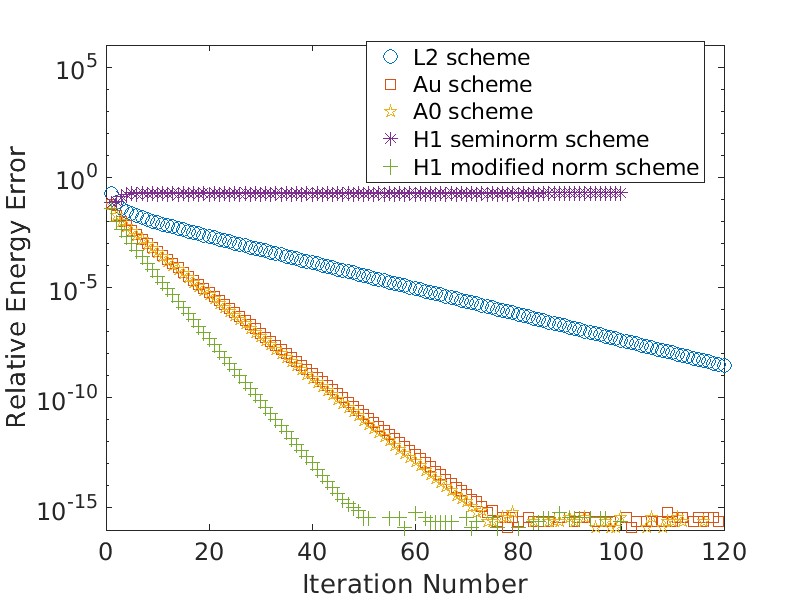
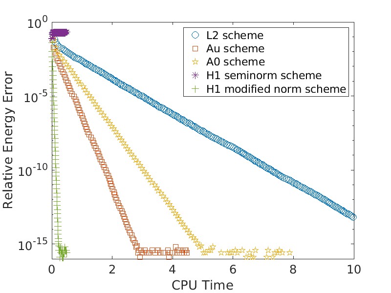
We consider the 2D problem with on the region . The performance of different gradient flow algorithms with fixed step size is shown in Figure 1. See [henning2020sobolev] and references therein for the definition of these schemes. We emphasize that these algorithms could be faster with different step sizes, e.g., the flow will be faster with a larger step size, and algorithm can be faster with adaptive step size. Here we just use the same step size to compare them. Notice that only needs to be applied twice in the modified gradient flow (4.4). In each iteration of , and schemes, one needs to invert matrices like or , which is much more expensive than computing [liu2023simple]. As shown in Figure 1, (4.4) with a proper parameter is quite efficient.
6.3. Comparison with the Backward Forward Euler method
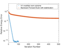
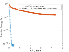
The modified flow has the advantage of inverting only constant coefficient Laplacian, which can be easily accelerated on modern GPUs as shown recently in [liu2023simple]. On the other hand, in the literature, there are similar schemes, e.g., the Backward Forward Euler method with a stabilization parameter in [bao2006efficient] is given by
| (6.2) |
The modified flow is very different from (6.2). For instance, (4.4) is a Riemannian gradient descent method. In particular, only one inversion of Laplacian is needed in each step of (6.2), but there are two inversions of Laplacian in (4.4). The optimal parameter for (6.2) was given in [bao2006efficient], yet it is unclear what the optimal should be for the modified flow. In numerical tests, the modified flow performs better when using tuned , see Figure 2.
6.4. Tuning parameters
We consider with a potential:
| (6.3) |
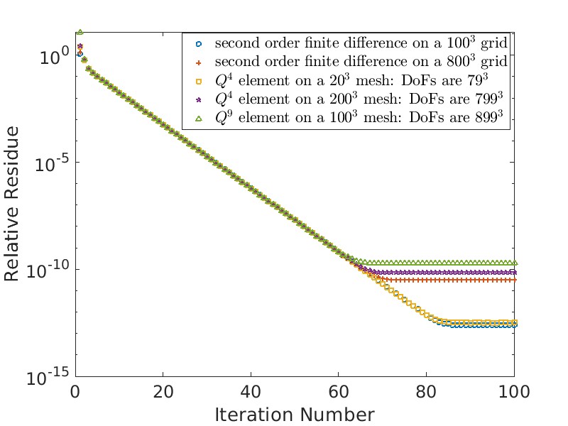
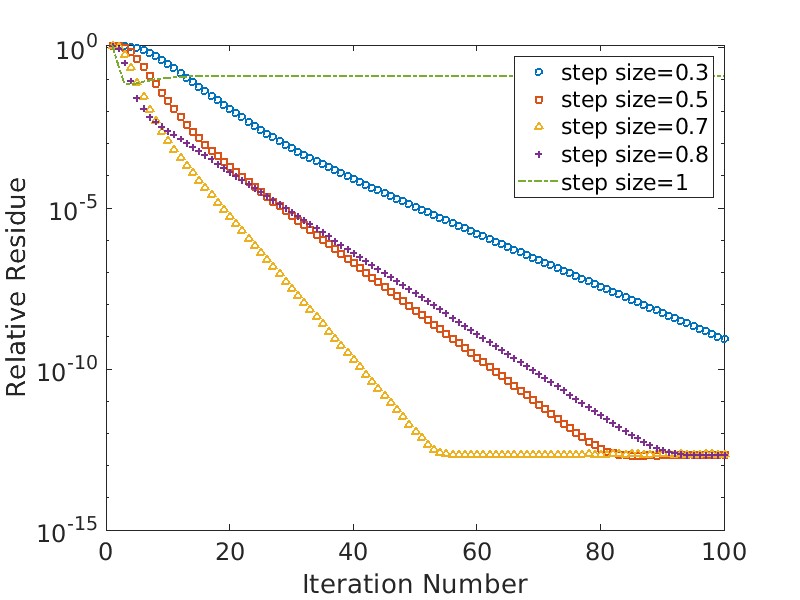
For (6.3) and , the modified scheme (4.4) with and has the same convergence performance for any grid size or any discrete Laplacian, unless it is an extremely coarse grid, as shown in Figure 3 (a). Thus we can easily find the best step size for a given by tuning it on a grid as shown in Figure 3 (b).
6.5. 3D implementation on GPUs
As shown recently in [liu2023simple], any discrete Laplacian on a Cartesian grid can be easily accelerated on modern GPUs with a simple implementation in MATLAB 2023. In particular, to invert a discrete Laplacian on a grid size , it only takes 0.8 seconds on one Nividia A100 GPU card. And such a result holds for spectral element method, see [liu2023simple] for details.
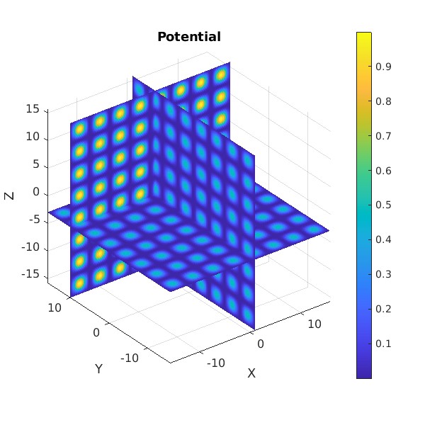
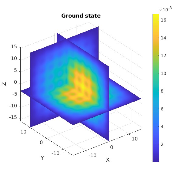
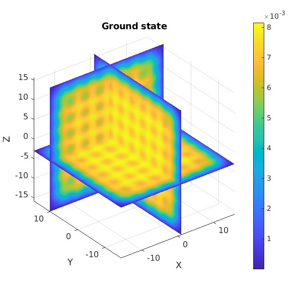
We consider solving the 3D problem with potential (6.3). See Figure 4 for visualization of the potential and its ground state for and . We define the online computation time as the computational time without counting the offline computational time such as preparing discrete Laplacian matrices and loading data to the GPU. For the potential (4) with , the modified flow scheme (4.4) with and , we stop the iteration when the relative residue stops decreasing, where the relative residue is defined as
The results of computing energy and the eigenvalue are listed in Table 2, in which GPU time is the online computational time. In particular, the online computation time is 214 seconds on the Nvidia A100 for 100 iterations of (4.4) on a grid. For , we use step size and , we stop the iteration when the relative residue stops decreasing. The performance is listed in Table 3. In both Table 2 and Table 3, the reference solutions are generated by spectral element method on a mesh, and the ground state errors are measured only at the nodes of matching with nodes of elements a mesh. For instance, for element on a mesh, is measured only at the cell vertices.
| The second order finite difference | ||||||
| DoFs | Mesh size | Iteration # | GPU time | |||
| 3.70E-4 | 3.72E-4 | 8.04E-4 | 86 | 0.88 second | ||
| 1.48E-5 | 1.48E-5 | 3.21E-5 | 76 | 165 seconds | ||
| The fourth-order compact finite difference | ||||||
| 1.17E-6 | 1.18E-6 | 2.00E-6 | 84 | 0.92 second | ||
| 1.86E-9 | 1.87E-9 | 3.21E-9 | 73 | 161 seconds | ||
| spectral element method | ||||||
| DoFs | FEM Mesh | Iteration # | GPU time | |||
| 8.57E-10 | 8.62E-10 | 2.73E-7 | 83 | 0.88 second | ||
| 3.60E-12 | 3.62E-12 | 4.86E-9 | 78 | 6.10 seconds | ||
| spectral element method | ||||||
| 3.53E-9 | 3.49E-9 | 6.06E-7 | 88 | 0.54 second | ||
| spectral element method | ||||||
| 5.31E-12 | 5.23E-12 | 1.29E-8 | 83 | 0.54 second | ||
| 8.79E-12 | 8.85E-12 | 6.42E-12 | 75 | 0.82 second | ||
| The second order finite difference | ||||||
| DoFs | Mesh size | Iteration # | GPU time | |||
| 5.67E-6 | 7.82E-6 | 2.96E-5 | 48 | 105 seconds | ||
| The fourth-order compact finite difference | ||||||
| 5.67E-10 | 8.72E-10 | 2.77E-9 | 48 | 106 seconds | ||
| spectral element method | ||||||
| DoFs | FEM Mesh | Iteration # | GPU time | |||
| 2.64E-10 | 4.06E-10 | 2.81E-7 | 54 | 0.63 second | ||
| 1.79E-12 | 2.33E-12 | 4.45E-9 | 50 | 3.88 seconds | ||
| spectral element method | ||||||
| 7.49E-8 | 6.44E-8 | 2.18E-7 | 57 | 0.42 second | ||
| spectral element method | ||||||
| 3.43E-12 | 4.07E-12 | 8.32E-9 | 54 | 0.37 second | ||
| 3.58E-12 | 4.96E-12 | 3.22E-12 | 50 | 0.57 second | ||
6.6. A 3D example with a combined harmonic and optical lattice potential
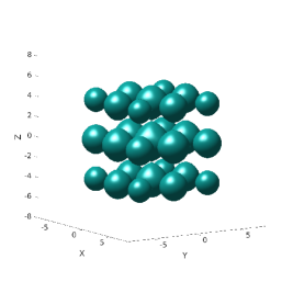
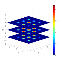
We consider the 3D example in [bao2006efficient] with the following combined harmonic and optical lattice potential on the domain :
For , we find that and are efficient parameters. The modified flow with spectral element method on a finite element mesh converges with residue reaching after 665 iterations using a simple and crude initial guess . The online computation time is 6 seconds on Nvidia A100. The numerical ground state energy and eigenvalue are and . The results are consistent with findings in [bao2006efficient]. Due to the different definitions of energy functions in this paper and [bao2006efficient], , and in this paper, correspond to the case for , and in [bao2006efficient]. See Figure 5.
7. Concluding remarks
We have considered the Sobolev gradient flow for finding the ground state of the Gross-Pitaevskii eigenvalue problem, under a modified -norm. Global convergence to a critical point and the local exponential convergence rate have been established. Numerical experiments suggest that the scheme with the spectral element method can be very efficient when using tuned parameters, which can be easily and efficiently implemented on modern GPUs.
References
Appendix A Explicit finite difference formulation and discrete energy
A.1. The explicit finite difference formulation
We give explicit equivalent finite difference formulation of the spectral element scheme (2.7), especially the case, which is equivalent to the second order finite difference.
A.1.1. The second order finite difference scheme
For a one-dimensional uniform grid with grid spacing , for any vector with polynomial basis, it can be represented by with . The discrete inner product is given by
Define and where . Then the matrices in (2.6) and (2.7) for 1D are , , and
For a two-dimensional problem on a uniform grid for the domain , assume there are interior grid points. Let , and denote 2D arrays of size consisting of point values of at grid points. Let be the vector generated by arranging column by column. The scheme (2.6) becomes
where denotes the entrywise cubic power. In 2D, (2.7) can be written as
With the property , it can be equivalently expressed as
where represents Hadamard product, i.e., entrywise product. With similar notation as in [liu2023simple], the three-dimensional case of (2.7) can be expressed as
Thus, the matrix is given explicitly as follows:
| (A.1) |
Remark A.1.
The scheme with quadrature gives exactly the same second-order centered difference for the interior grid. For Neumann boundary condition, the scheme with quadrature gives a slightly different scheme from a conventional finite difference scheme, see Remark 3.3 in [10.1093/imanum/drac014]. When deriving finite difference from the finite element method, convergence is trivially implied by finite element error estimates.
A.1.2. The discrete Laplacian from scheme
The full detail can be found in [liu2023simple]. Let be the stiffness matrix and be the mass matrix spectral element method in one dimension. In two dimensions (2.6) can be written as
Define , the scheme (2.7) in two dimensions can be written as
or equivalently and in three dimensions it is
It is possible to derive explicit entries of matrices , see [li2020superconvergence, shen2022discrete] for more details.
Remark A.2.
For , the discrete Laplacian above give a -th order finite difference scheme in discrete -norm for solving elliptic equations [li2020superconvergence] and for parabolic, wave and Schrödinger equations [li2022accuracy]. For solving a linear eigenvalue problem, e.g., in (2.7), standard a priori error estimates for eigenvalues is that spectral element method gives -th order of accuracy if assuming sufficient regularity.
A.2. Discrete energy of the second order scheme
For the one-dimensional case, recall that for , we have
Define the matrix Then it satisfies . In one dimension . Thus we have
In two dimensions, by plugging in the quadrature, for any , we have
| (A.2) |
With our notation for the two-dimensional problem, let , then we have
The three-dimensional case of the discrete gradient can be similarly written out.
Appendix B M-matrix and Perron-Frobenius theorem
B.1. M-matrix
Nonsingular M-matrices are monotone. There are many equivalent definitions or characterizations of M-matrices, see [plemmons1977m]. The following is a convenient sufficient but not necessary characterization of nonsingular M-matrices [li2019monotonicity]:
Theorem B.1.
For a real square matrix with positive diagonal entries and non-positive off-diagonal entries, is a nonsingular M-matrix if all the row sums of are non-negative and at least one row sum is positive.
B.2. Irreducible nonnegative matrices
A matrix is called reducible if there exists a permutation matrix such that is block upper triangular. A matrix is irreducible if and only the graph it represents is strongly connected.
Lemma B.2.
For a nonsingluar irreducible matrix , is also irreducible.
The following results can be found in [varga1999matrix]:
Theorem B.3 (Perron-Frobenius).
If is irreducible, then:
-
(1)
The spectral radius is a simple eigenvalue of with an eigenvector .
-
(2)
increases when any entry of increases.
Theorem B.4.
The positive eigenvector (Perron-Frobenius eigenvector) for an irreducible nonnegative matrix is unique up to scalar multiplication.
Proof.
Let be the left Perron-Frobenius eigenvector then . If there exists another eigenvector for an eigenvalue , then . Since , we get and . Thus there is only one eigenvalue, i.e., , with positive eigenvectors, and is a simple eigenvalue by Theorem B.3. ∎
Appendix C Deferred proofs for Section 5.1
C.1. Norm equivalence and standard regularity results
Lemma C.1.
There are positive constants independent of mesh size , such that the followings hold for any :
| (C.1) |
Proof.
Consider a cubic cell and a reference cell . For defined on , consider , which is defined on . Let denote the approximation to the integral by -point Gauss Lobatto quadrature for each variable. Since both and are norms of , by the equivalence of any two norms on the finite-dimensional space , we have
By mapping back to , and summing over , we get (C.1) for .
With the same notation and arguments above, for a polynomial with -point Gauss-Lobatto quadrature, let and be quadrature weights and quadrature node values on the reference cell , then we have , which can be easily verified to be a norm of thus a norm of . By the equivalence of any two norms on , we have
By mapping back to , and summing over , we get (C.1) for . The proof of is almost identical to the case . ∎
Second, we want to show the -norm is equivalent to -norm for piecewise polynomials in . By Lemma 5.1 in [li2020superconvergence], we have the following standard -ellipticity result for a domain on which elliptic regularity holds, e.g., .
Lemma C.2.
Let . Let be a domain with elliptic regularity. There is a constant independent of mesh size s.t.
| (C.2) |
C.2. Proofs of lemmas in Section 5.1
Proof of Lemma 5.4.
Proof of Lemma 5.5.
(i) .
(ii) By Cauchy-Schwartz inequality for the inner product and (i), we get
|
|
Proof of Lemma 5.6.
Proof of Lemma 5.7.
It can be computed that
which leads to
∎
Appendix D Deferred proofs for Section 5.2
Proof of Lemma 5.11.
Since is self-adjoint w.r.t. , it has orthonormal eigenvectors. Let be the orthogonal projection of onto the subspace spanned by . Let , then and . Thus,
With the following fact, (5.5) follows from the estimate above:
∎
Lemma D.1.
There is some constant independent of the mesh size s.t.
Proof.
Lemma D.2.
For any with and , it holds for some constant depending on and independent of the mesh size that
Appendix E Positive eigengap independent of the mesh size
In this section, we prove that Assumption 5.8 holds with a positive eigengap independent of the mesh size for the scheme with .
E.1. Technical lemmas
Lemma E.1.
Suppose that . There exist constants independent of the mesh size, so that for any and , the followings hold
-
(i)
.
-
(ii)
.
-
(iii)
.
-
(iv)
.
Proof.
It suffices to prove the results on each rectangle of the grid, since all of them are additive. Without loss of generality, consider only the rectangle and . The result (i) follows from the following:
The result (ii) can be derived as follows:
where we used (i). The result (iii) is true since
Finally, the result (iv) is a consequence of Jensen’s inequality :
∎
Lemma E.2.
For any and , it holds for some constant independent of the mesh size that .
Proof.
According to the calculation in the proof of Lemma E.1 (iii), we have
and
We can conclude the proof after combining the estimates above and the following consequences of the Bramble-Hilbert Lemma (see [li2020superconvergence, li2020-coef]):
∎
Lemma E.3.
Let be some piecewise constant interpolation of the piecewise linear function , then there is some constant independent of the mesh size s.t.
Proof.
Without loss of generality, consider a rectangle and suppose that and on . The desired inequality follows immediately from
∎
E.2. Proof of consistency and eigengap
Theorem E.4.
Let and be the ground state and the corresponding eigenvalue of the continuous energy . Let and be the ground state and the corresponding eigenvalue of the discrete energy . Suppose that and that . Then in and as .
Proof.
By our previous notation, is the vector collecting the values of at quadrature points and . For convenience, define as the vector representing the values of at quadrature points. Due to the embedding for and the convergence of Riemannian integral for continuous functions, one has , , and . Furthermore, thanks to Lemma E.2, we have . Then it holds that
| (E.1) |
which implies that is bounded as .
By Lemma E.1 (i) and boundedness of , one has . Therefore, it follows from Lemma E.1 (ii)-(iv) that
| (E.2) |
By compact embeddings and , there exists a subsequence of the bounded sequence converging weakly in and strongly in and to some function in . Without loss of generality, we assume that the whole sequence converges:
Since the week convergence guarantees that ,
which implies that and hence that by the uniqueness of positive ground state. Then we know that weakly in and . Note that the weak convergence and convergence of norm imply the strong convergence. Thus and strongly in .
In the discussion above, we have shown that every subsequence of has a subsequence that converges strongly in to . Therefore, the whole sequence converges strongly in to . This immediately implies that . ∎
Assumption E.5.
We assume that the multiplicity of the eigenvalue to the following problem is one: .
Theorem E.6.
We remark that in Theorem E.6 is exactly in Assumption 5.8. In this sense Theorem E.6 validates Assumption 5.8 with a positive lower bound for the eigengap that is independent of the mesh size .
Proof of Theorem E.6.
Suppose that there is no positive eigengap. Then when passing to a subsequence. Notice that
| (E.3) |
which implies the boundedness of , where and we used Lemma E.1 (iii). There exists such that converges to , a.e., weakly in , and strongly in and , when passing to another subsequence.
Let us analyze the limiting behavior of each term in (E.3). It follows from the weak convergence in that
By Fatou’s lemma and Lemma E.1 (ii), one has
Let and be the piecewise constant approximation of and in the sense of the one in Lemma E.3, then
which implies and a.e. when passing to a subsequence. By Fatou’s lemma, it holds that
Then taking limit for (E.3) as , one obtains that
where the last equality follows from by Lemma E.1 (i) and strongly in . This implies that is also a ground state of the linearized problem at . However, one has from Lemma E.1 (i) that
which implies that , leading to a contradiction. ∎