Are Classification Robustness and Explanation Robustness Really Strongly Correlated? An Analysis Through Input Loss Landscape

Abstract

This paper delves into the critical area of deep learning robustness, challenging the conventional belief that classification robustness and explanation robustness in image classification systems are inherently correlated. Through a novel evaluation approach leveraging clustering for efficient assessment of explanation robustness, we demonstrate that enhancing explanation robustness does not necessarily flatten the input loss landscape with respect to explanation loss - contrary to flattened loss landscapes indicating better classification robustness. To deeply investigate this contradiction, a groundbreaking training method designed to adjust the loss landscape with respect to explanation loss is proposed. Through the new training method, we uncover that although such adjustments can impact the robustness of explanations, they do not have an influence on the robustness of classification. These findings not only challenge the prevailing assumption of a strong correlation between the two forms of robustness but also pave new pathways for understanding relationship between loss landscape and explanation loss.

Keywords Classification Robustness  $\cdot$ Explanation Robustness  $\cdot$ Loss Landscape

1 Introduction

In deep learning, the robustness of image classification systems against adversarial instances has emerged as an important area of research. These systems, integral to modern artificial intelligence, frequently encounter scenarios where adversarial instances—subtly altered images designed to deceive algorithms—pose significant challenges. At the heart of this challenge lie two critical concepts: classification robustness and explanation robustness. Classification robustness refers to a model’s ability to maintain accuracy under adversarial attacks [1, 2], while explanation robustness pertains to the consistency of the model’s interpretative outputs in such adversarial scenarios [3, 4]. Traditionally, there’s been a prevailing conclusion within the research community [5, 4]:

Conclusion: Classification robustness and explanation robustness are strongly correlated: Increasing classification robustness can increase explanation robustness and vice versa.

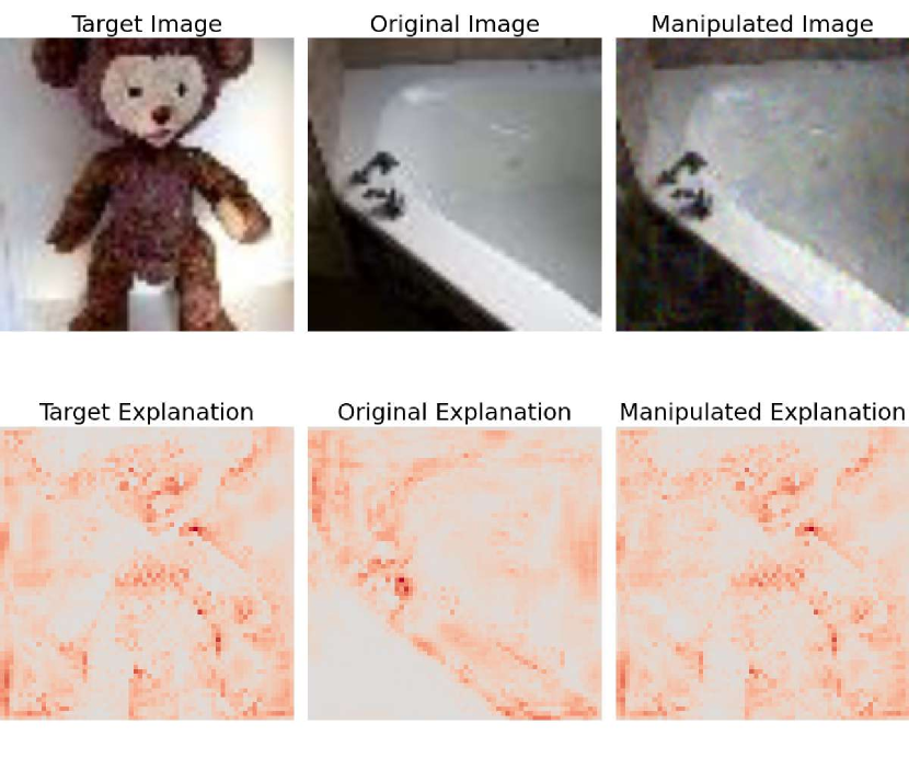
(a) Example of adversarial attack on explanation. The explanation maps of original image can be manipulated to the target explanation.

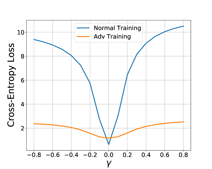
(b) Comparison of input loss landscapes between normal and adversarially trained models on CIFAR-10 shows that the adversarially trained models have much flatter landscapes. Adversarial training can increase classification robustness.

Figure 1: (a) Illustration of an adversarial attack on explanation, demonstrating the manipulation of explanation maps from the original image to achieve a target, resulting in explanation loss (b) A visualization of input loss landscape w.r.t classification loss, comparing a normal-trained model to an adversarial-trained model.

This paper, however, unveils a finding that disrupts this conventional belief: a notable contradiction in the assumed correlation between classification robustness and explanation robustness. This revelation not only challenges established assumptions but also opens new avenues for understanding and improving the resilience of deep learning models.

Adversarial attacks on classification aim at deceiving image classification models by introducing perturbations to benign images [1]. To defend against adversarial examples, adversarial training (AT) [2, 6] is one of the most effective approaches which explicitly augments the training process to enhance a model’s inherent robustness against adversarial samples for classification. Classification robustness typically is referred as the classification accuracy under adversarial attacks, and AT methods are effective in improving the classification robustness of a deep learning model.

Explanation maps [7], also known as saliency maps, are proposed to explain deep learning methods by feature importance. However, explanation maps are themselves also vulnerable to adversarial attacks [3, 8]. For example, in Figure 1(a), by making small visual changes to the input sample which hardly influences the network’s output, the explanations can be arbitrarily manipulated [3]. Explanation robustness is referred as the error between victim explanation under adversarial attacks on the input and targeted explanation.

To better understand robustness, one important way is to explore the input loss landscape [9]. Existing work has found out that a flat input loss landscape w.r.t classification loss indicates better classification robustness [10, 9], as shown in Figure 1(b). To visualize the input loss landscape, we add the random perturbation to the inputs with magnitude $\alpha$ (detailed visualization method can be found in Section 3). The results in Figure 1(b) show that models with higher classification robustness have a flatter input loss landscape w.r.t classification loss.

Then a natural question comes up for explanation robustness:

Q: Does increasing explanation robustness of a model also flatten input loss landscape w.r.t explanation loss?

We visualize the input loss landscape w.r.t explanation loss in Figure 3 using models with different levels of explanation robustness and find that, surprisingly, increasing the explanation robustness does not flatten the input loss landscape w.r.t explanation loss. Specifically, to obtain models with different levels of explanation robustness, we consider utilizing adversarial training methods that allow us to control the emphasis on classification robustness [11] since previous works have proven that increasing classification robustness can also increase explanation robustness.

The previous observation that increasing the explanation robustness does not flatten the input loss landscape w.r.t explanation loss is strange compared with increasing classification robustness could flatten the input loss landscape w.r.t classification loss. To further explore this observation, we ask the previous question in a reverse way:

Q: Does flattening the input loss landscape w.r.t explanation loss not increase the robustness of explanations as well?

The answer to this question is, flattening the input loss landscape w.r.t explanation loss will decrease the explanation robustness. Specifically, we propose a new loss function to flatten the loss landscape w.r.t explanation loss. The results show that adding the loss will decrease the explanation robustness but not change the classification robustness measured by adversarial accuracy. This observation, indicating that influencing explanation robustness does not impact classification robustness, challenges the previous conclusion: the correlation between explanation robustness and classification robustness may not hold.

Overall, we summarize our contributions as follows:

• We propose a sampling method based on cluster methods that can choose representative pairs to evaluate explanation robustness more efficiently.

• We use TRADES [11] to control the classification robustness and explanation robustness and visualize the input loss landscape w.r.t explanation loss to find that increasing the explanation robustness by increasing the classification robustness does not flatten the input loss landscape.

• We propose a new training method that flattens the input loss landscape w.r.t explanation loss. The training results show that explanation robustness may not be strongly correlated to classification robustness.

2 Related Work

Adversarial Attack and Adversarial Training (AT) It has been proven that convolutional neural networks (CNNs) are vulnerable to the adversarial examples [1, 6, 12]. Noise that is imperceptible to humans, when added to the original inputs, can lead to the misclassification of models. Projected Gradient Descent (PGD) [2] is one of the most popular methods that generate such a noise or evaluate models’ classification robustness by calculating accuracy under its attack. Many methods have been introduced to defend against adversarial attacks including knowledge distillation [13], quantization [14, 15] and noise purification [16, 17]. However, these preprocessing methods do not involve a training process and may be vulnerable to adaptive attack [18]. Goodfellow et al. [6] first introduced adversarial training (AT), which trains a model from scratch with adversarial samples. Adversarial Training (AT) proved its performance including adversarial competitions [2, 19]. In our paper, we also focus on classification robustness increased by AT.

Many works tend to increase the performance of AT through external datasets [20, 21, 22], metric learning [23], self-supervised learning [24], ensemble learning [25], label smoothing [26] and Taylor Expansion [27]. Wu et al. [28] found that obtaining a flat loss landscape can help increase classification robustness, which inspired the ideas in this paper. There is also a line of work that attempts to accelerate AT. For example, Shafahi et al. [29] reused calculated adversarial noises, Liu et al. [30] introduced single-step training and TRADES [11] selects training samples by largest Kullback–Leibler (KL) divergence between adversarial data and normal data. In this paper, we mainly consider the Madry adversarial training [2].

Explanation Robustness Saliency maps [31, 32, 33, 34] are widely used to explain image-related tasks in deep learning, and our focus is on the robustness of these explanations. However, similar to an adversarial attack, it is possible to find an adversarial noise on original images so that it can easily manipulate the saliency maps without changing classification results in both white-box [3, 8, 35, 36] and black-box settings [37]. Zhang et al. [38] further introduced a new method that can attack both saliency maps and classification results. In order to evaluate the explanation robustness, Wicker et al. [39] introduced the max-sensitivity and average-sensitivity of saliency maps. Alvarez et al. [40] estimated explanation robustness by the Local Lipschitz of interpretation while Tamam et al. [37] directly used attack loss to evaluate explanation robustness. In this paper, we use attack loss based on the proposed cluster method to evaluate explanation robustness.

Several works have also aimed to improve explanation robustness. Chen et al. [41] introduced a regularization term during training to make the explanation more robust. Boopathy et al. [5] improved the performance by training with noisy labels. Tang et al. [42] proposed a first-order gradient-based approach to reduce computational training costs. Huang et al. [4] explored genetic algorithms to optimize explanation robustness.

Relationship between Classification Robustness and Explanation Previous works have demonstrated that a good explanation is crucial for classification robustness [43, 44], suggesting that a better saliency map correlates with improved classification robustness. Follow-up work by Boopathy et al. [5], Tang et al. [42] and Huang et al. [4] further demonstrated when models are more robust to attacks manipulating explanations, their robustness to classification attacks also improves and vice versa. Therefore, increasing explanation robustness can benefit classification robustness.

In our paper, we prove that improving explanation robustness indeed also boosts classification robustness, specifically under adversarial training regimes using TRADES [11]. However, through further analysis, we prove these two facets of robustness are not inherently the same - they can be disconnected. Classification robustness is not fundamentally vital for explanation robustness.

3 Loss Landscape Visualization

In this section, we outline our strategy for obtaining models with varying levels of explanation robustness and detail our method for visualizing the input loss landscape. Past research has demonstrated a correlation between increased classification robustness and enhanced explanation robustness [4]. To achieve models with a spectrum of classification robustness levels, we employ adversarial training, specifically adopting TRADES [11], a technique that offers detailed control over classification robustness. In contrast to previous methods like Madry adversarial training [2], where the decision is limited to determining whether to enhance classification robustness, TRADES provides a precise approach, allowing us to regulate the level of classification robustness in our experiments.

Background of TRADES TRADES [11] is an adversarial training technique that enables controllable emphasis on improving classification robustness. Specifically, the TRADES training loss is:

$$L_{Tra}=L_{sc}(f(x),y)+\alpha L_{adv}(f(x),f(x_{adv})),$$ (1)

where $f(x)$ is the output from trained model by given input $x$, $L_{sc}(f(x),y)$ is the standard classification loss like cross-entropy between the model output $f(x)$ and label $y$, $x_{adv}$ is an adversarial example crafted from $x$ using an attack method like PGD [2] or AutoAttack [45]. $L_{adv}$ stands for adversarial loss and it computes the Kullback-Leibler (KL) divergence between the original and adversarial representations, and $\alpha$ controls the importance given to promoting classification robustness. With $\alpha=0$, TRADES defaults to normal training. As $\alpha$ increases, a model trained with TRADES shows increased classification robustness. The tunable $\alpha$ allows precisely getting models with different levels of classification robustness and explanation robustness.

Explanation Loss To visualize the explanation loss, we need to know what is explanation loss. Most white-box and black-box adversarial attacks on explanation contain an explanation loss to guide the attack. Specifically, let $I$ represent the explanation method, $x_{t}$ the target images, and $x_{v}$ the victim images; then, the respective saliency maps are $I(x_{t})$ and $I(x_{v})$. Adversarial attacks on explanation aim at finding a noise $\epsilon$ where:

$$\epsilon=\arg\min_{\epsilon}\lVert I(x_{v}+\epsilon)-I(x_{t})\rVert.$$ (2)

Therefore, in this paper, we formally define the explanation loss as:

Definition 1 (Explanation Loss).

$\mathcal{L}_{e}(x_{v}+\epsilon,x_{t})=\lVert I(x_{v}+\epsilon)-I(x_{t})\rVert$.

To prevent $\epsilon$ from being too large, Dombrowski et al. [3] and Tamam et al. [37] utilize an additional classification loss to ensure that the manipulated images yield the same classification results as the original images.

Explanation Robustness Evaluation To determine whether we really get models with different explanation robustness, we introduce how we measure explanation robustness here. Since there is an explicit attack target $\mathcal{L}_{e}$, a natural idea is to directly use the explanation loss after the attack to measure the models’ explanation robustness. However, it is nearly impossible to calculate explanation loss $\mathcal{L}_{e}$ for every pair in the dataset. For example, the test set of CIFAR10 [46] contains 10k images, which leads to nearly 100M pairs for victim and target images. Attacking every pair would be an exceedingly time-consuming task.

To ensure an efficient and effective evaluation, we aim at choosing the most representative subset from the original test leveraging clustering methods such that images within the same cluster have similar explanations. Then we can choose images from each cluster with the closest distances to cluster centroids. In detail, we cluster images based on the output from the last layer before the classification layer of a normal pre-trained ResNet18 [47] with k-means [48] and $k=10$. In our approach, clustering is applied to pre-trained feature spaces, bypassing the direct use of class labels to create pairs of images, which form inter-cluster and intra-cluster pairs. An intra-cluster pair means that the victim and target images from a pair are both from the same cluster, whereas an inter-cluster sample consists of images from different clusters. In this way, clustering ensures that intra-cluster pairs share similarities in explanations. In other words, our clustering method aims at finding the most representative subset w.r.t explanation. we visualize the saliency maps (explanation) in Figure 3. We can see that two images from the same cluster3, even though these two images are from different classes, show a similar explanation while both of their explanations are quite different from the image from the other cluster.

In the rest of the paper, we choose 15 images from each cluster and form a subset $\mathcal{D}_{e}$ of the test set for each dataset. $\mathcal{D}_{e}$ contains 150 images and $150\times 149=22,350$ pairs. We report the mean explanation loss for all pairs in $\mathcal{D}_{e}$ to evaluate explanation robustness in the rest of the paper. We use a white-box attack from Dombrowski et al. [3] as the explanation attack method in our paper.

Analysis In Table 1, we provide an evaluation of classification robustness and explanation robustness for models trained with TRADES and different $\alpha$ on CIFAR10. From Table 1, it is easy to see that, with the increase of $\alpha$, both the classification and explanation robustness of the model increase. Therefore, we obtain models with different explanation robustness.

Table 1: Comparison of classification robustness and explanation robustness of models trained with TRADES and different $\alpha$ on CIFAR10. The results show that within a certain range, using the TRADES training method and increasing the value of $\alpha$ can not only improve the classification robustness but also improve the explanation robustness.

Metric	Expl at Start($1e-7$)	Expl at End	Clean Acc(%)	Adv Acc(%)
$\alpha$	Explanation Robustness		Classification Robustness
0	10.375	6.206	79.08	0.00
0.5	16.635	10.640	75.60	23.57
1.0	17.271	10.946	72.63	28.31
2.0	17.290	10.965	69.56	31.77
4.0	18.004	11.293	65.63	33.28
5.0	18.278	11.469	64.50	33.98
10.0	18.643	11.592	60.26	34.87

Visualization After getting the models with different explanation robustness, the next step is to visualize input loss landscape w.r.t explanation loss. We visualize the input loss landscape by plotting the change of explanation loss when we add a random noise $\mathbf{d}$ to the victim image $x_{v}$ with different magnitude $\gamma$:

$$f(\gamma)=\mathcal{L}_{e}(x_{v}+\gamma\mathbf{d},x_{t}),$$ (3)

where $\mathbf{d}$ is sampled from a standard Gaussian distribution. We provide the mean explanation loss for all pairs in the subset we build, with the results displayed in Figure 3. We can see that the adversarially trained models have better explanation robustness because of the high initial explanation loss instead of a flat loss landscape. We also visualize compared with normal training and Madry adversarial training (MAT) in Appendix Figure 7, and it shows similar results: increasing explanation robustness will not flatten the input loss landscape w.r.t explanation loss. In the area of classification robustness, previous work has proven that a model with good classification robustness has a flat loss landscape w.r.t classification loss [10, 9]. However, different from the conclusions drawn in classification robustness, adversarially trained models don’t exhibit a flat loss landscape w.r.t explanation loss. This phenomenon motivates us to propose the method in the following section to flatten the input loss landscape w.r.t explanation robustness.

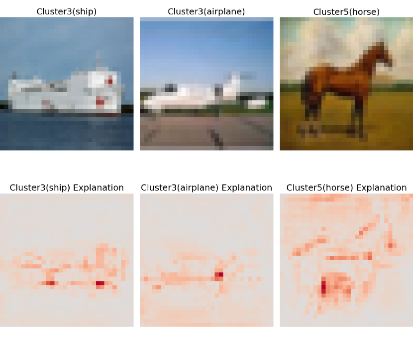
Figure 2: The explanations from different clusters generated by our clustering method on CIFAR10. The two images with different labels in the same cluster share a similar explanation while they both show a different explanation with the image from another cluster. The results show that our method can pick the most representative images w.r.t explanation.

Figure 3: Input Loss landscape w.r.t explanation loss for models trained with different with different $\alpha$ in TRADES. The results show that the loss landscape w.r.t explanation robustness does not show a clear difference between models that vary in explanation robustness.

4 Methods

In the previous section, we observe a strange situation where increasing the explanation robustness does not flatten the input loss landscape w.r.t explanation robustness. To further explore this situation, we consider this situation in a reverse way: How Does flattening the input loss landscape w.r.t explanation loss influence the robustness of explanations? In this section, we propose a new training algorithm to flatten the input loss landscape w.r.t explanation robustness. To explicitly guide the training with flattening input loss landscape w.r.t explanation robustness, we decide to add an extra loss:

$$\mathcal{L}_{f}=\lVert I(x+\zeta)-I(x)\rVert,$$ (4)

where $\zeta$ is a noise randomly sampled from a standard Gaussian distribution and $I$ is the explanation method. We use randomly sampled noise within a standard training framework instead of the min-max training framework used in the previous flatness-aware methods [28] because flat training methods based on AT [28] typically use an untargeted setting while off-the-shelf explanation adversarial attacks must be executed in a target setting. A victim image and a target image are required for the explanation of adversarial attacks [37, 3]. Besides, calculating $\zeta$ through a targeted setting may increase the training time and increase the probability that the model is overfitting to the chosen pairs.

It is important to note that the new loss function $\mathcal{L}_{f}$ can be incorporated into any training framework, including Madry adversarial training [2], TRADES [11], and normal training. We will mainly focus on Madry adversarial training plus the new training loss:

$$\mathcal{L}=\mathcal{L}_{sc}(f(x_{adv}),y)+\lambda\mathcal{L}_{f}.$$ (5)

In Equation 5, we use the hyperparameter $\lambda$ to balance two components of the loss. Here $\lambda$ can be both positive which guides the loss landscape to become flat and negative which leads to a sharper loss landscape. We allow $\lambda$ to take both positive and negative values to enable a more comprehensive analysis of the loss landscape. According to the experimental results, our new method shows that our method can influence explanation robustness while it does not change classification robustness. Since we obtain $x_{adv}$ based on PGD, we name our new training method with Separate Explanation robustness with PGD ($SEP$). We denote the method as $SEP_{pos}$ when $\lambda$ is positive, and as $SEP_{neg}$ when $\lambda$ is negative. We summarize our algorithm in Algorithm 1. We also visualize the comparison of saliency maps from models trained with different algorithms to provide how our methods influence the saliency maps in Figure 4.

Algorithm 1 Separate Explanation Robustness with PGD($SEP$)

1:  Input: Dataset $\mathcal{D}$, total training iteration $T$, explanation method $I$, model weights $\mathbf{w}$, and balancing factor $\lambda$.

2:  for $t=0$ to $T-1$ do

3:     for batch $x$ in $\mathcal{D}$ do

4:        Sample a random noise $\zeta$ from a standard Gaussian distribution.

5:        Get adversarial samples (On classification): $x_{adv}=PGD(x,y)$.

6:        Calculate Loss function with Equation 5.

7:        Update $\mathbf{w}\leftarrow\mathbf{w}-\eta\nabla\mathcal{L}(f(x),f(x_{adv}),y|\mathbf{w})$

8:     end for

9:  end for

(a) $SEP_{pos}$

(b) $SEP_{neg}$

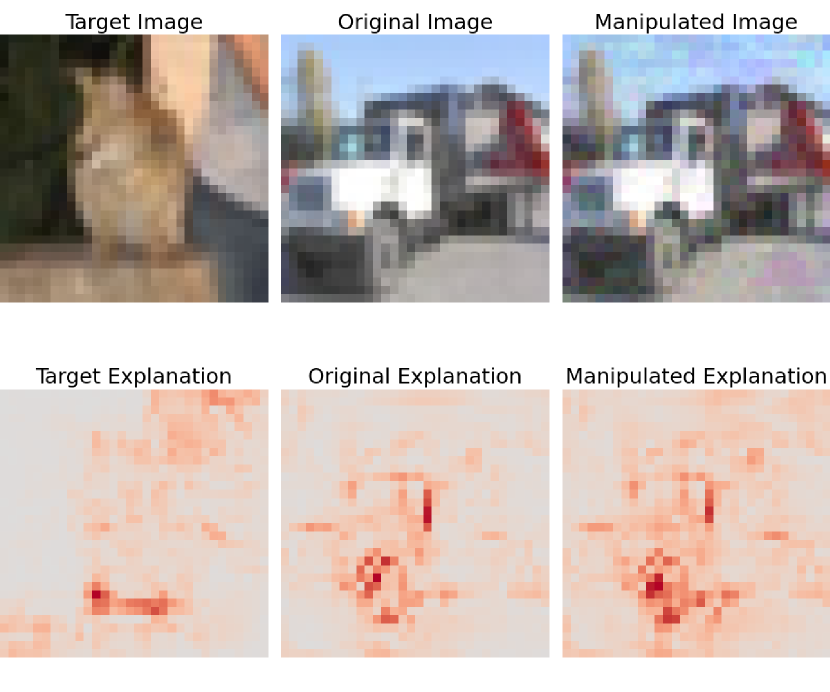
(c) Adversarial Training

Figure 4: How does our method influence the saliency maps calculated from gradient x inputs on CIFAR10. Intuitively, $SEP_{pos}$ makes the model consider more input pixels, solely adversarial training makes the model consider only a few input pixels while $SEP_{neg}$ considers even fewer input pixels compared with adversarial training. However, models trained with these three methods show the same classification robustness.

5 Experimental Results

In this section, we conduct verification experiments on multiple datasets and models to effectively demonstrate the ability of our proposed method to differentiate explanatory robustness from classification robustness.

5.1 Experimental Settings

Datasets

To thoroughly demonstrate the impact of our proposed training method and the resulting conclusions, we conduct model training on five publicly available datasets for experiments: CIFAR10 [46], CIFAR100 [46], MNIST [49], Fashion MNIST [50], and TinyImageNet [51]. Their detailed descriptions can be found in the Appendix.

Model Architecture

In addition to utilizing diverse datasets, we have also designed four distinct models for training on these datasets, further reinforcing our conclusions. We conduct experiments on ConvNet, ResNet [47], Wide ResNet [52] and MoblieNetV2 [53, 54]. The ConvNet model consists of three convolutional layers and one fully connected layer from Gidaris et al. [55]. For ResNet and Wide ResNet, we use a standard ResNet18 and Wide-ResNet-28, respectively. We also adjust the ResNet, Wide ResNet, and MoblieNetV2 so that they can fit into all datasets we use. All four models employ the softplus [56] activation function because it is better for the explanation attack method we use [3]. Since softplus is very close to the standard ReLU, changing the activation function does not influence the classification results too much.

Explanation Methods

We consider three explanation methods: Gradient[7], Gradient × Input[32], and Guided Backpropagation[57]. Gradients[7] are utilized to measure how small changes in each pixel affect the prediction. Gradient × Input[32] is an improvement of Gradient, which evaluates the contribution of each pixel to the prediction more precisely considering the original value of the input. Guided backpropagation[57] is a variation of gradient explanation where the negative component of the gradient is set to zero.

Training Methods

We mainly consider 2 baselines: i) normal training (Normal), ii) Madry adversarial training (MAT) [2]. As mentioned in the Section 4, we explore two types of proposed method: $SEP_{pos}$ and $SEP_{neg}$. In the rest of this paper, unless specified, we will use $\lambda=50000$ for $SEP_{pos}$ and $\lambda=-3000$ for $SEP_{neg}$.

Hyperparameters

For all experiments, we train our models 25 epochs with 64 as the batch size. To accelerate the training process, we use Adam [58] as the optimizer. We list the detailed hyperparameters for CIFAR10 in the Appendix Table 5. We use the standard settings in adversarial training [59], with $\epsilon=8/255$ in PGD for RGB images and $\epsilon=0.3$ for grayscale images, and steps in PGD are set to 10 for all experiments.

Metrics

As mentioned in Section 3, we report the explanation at end (after attack) to measure the explanation robustness. A higher explanation loss means a worse attack and thus better explanation robustness. We also include the explanation loss at start (before attack) to show the influence of our method on the explanation loss landscape. For classification robustness, we report the adversarial accuracy which is the classification accuracy under an adversarial attack. A higher adversarial accuracy shows better classification robustness. We also report clean accuracy to determine whether the models work normally in non-adversarial settings.

5.2 Separating Explanation and Classification Robustness

Table 2: Performance of models trained by ConvNet and ResNet18 on various data sets according to four training methods w.r.t. explanation loss at start, at end, and adversarial accuracy. A higher explanation loss at end, a better explanation robustness; a higher adversarial accuracy, and a better classification robustness. We also put explanation loss at start to show our method can influence the explanation robustness by influencing the explanation loss at start. The best performance in explanation robustness and classification robustness and the worst performance in explanation robustness are highlighted. There is no positive correlation between the model’s explanation robustness and classification robustness achieved through the $SEP_{pos}$ and $SEP_{neg}$ training methods, as compared to the MAT training method.

ConvNet					ResNet18
MNIST
Method	Expl at Start ($10^{-7}$)	Expl at End	Clean Acc(%)	Adv Acc(%)	Expl at Start	Expl at End	Clean Acc(%)	Adv Acc (%)
Normal	261.183	204.825	99.29	0.00	266.834	146.16	99.36	0.00
MAT	373.262	298.729	99.00	89.92	916.017	778.003	99.28	94.60
$SEP_{pos}$	93.033	61.545	98.8	89.4	92.371	59.278	98.4	91.63
$SEP_{neg}$	806.204	657.180	98.97	90.34	9356.306	8248.627	99.4	93.95
FMNIST
Method	Expl at Start ($10^{-7}$)	Expl at End	Clean Acc(%)	Adv Acc(%)	Expl at Start	Expl at End	Clean Acc(%)	Adv Acc (%)
Normal	106.530	72.198	92.32	0.00	128.640	69.847	91.57	0.00
MAT	386.370	274.267	62.85	73.98	588.610	417.031	79.22	67.1
$SEP_{pos}$	35.588	22.465	69.88	86.81	32.466	22.512	68.75	56.51
$SEP_{neg}$	1811.969	994.818	62.75	76.89	8050.942	7593.650	70.23	57.55
CIFAR10
Method	Expl at Start ($10^{-7}$)	Expl at End	Clean Acc(%)	Adv Acc(%)	Expl at Start	Expl at End	Clean Acc(%)	Adv Acc(%)
Normal	10.375	6.206	79.08	0.00	13.982	6.130	81.32	0.00
MAT	16.913	6.906	64.85	35.11	31.959	21.879	67.22	29.09
$SEP_{pos}$	3.565	1.269	64.94	35.25	11.962	7.958	66.68	29.69
$SEP_{neg}$	19.002	7.590	64.56	34.86	70.159	36.276	39.17	29.32
CIFAR100
Method	Expl at Start ($10^{-7}$)	Expl at End	Clean Acc(%)	Adv Acc(%)	Expl at Start	Expl at End	Clean Acc(%)	Adv Acc(%)
Normal	10.099	6.140	48.39	0.05	12.044	4.716	41.24	0.00
MAT	20.642	13.650	36.4	17.35	33.456	22.623	36.14	15.70
$SEP_{pos}$	13.650	9.932	37.41	17.98	19.217	12.744	34.83	15.16
$SEP_{neg}$	22.506	14.970	36.17	17.43	35.525	24.289	34.80	15.87
TinyImageNet
Method	Expl at Start ($10^{-7}$)	Expl at End	Clean Acc(%)	Adv Acc(%)	Expl at Start	Expl at End	Clean Acc(%)	Adv Acc(%)
Normal	0.966	0.633	28.71	0.00	1.131	0.528	28.34	0.00
MAT	2.426	1.728	25.13	9.55	3.119	2.349	26.34	10.81
$SEP_{pos}$	2.242	1.571	24.83	9.63	1.967	1.435	25.96	10.83
$SEP_{neg}$	3.873	2.610	24.31	9.61	4.413	3.016	26.11	10.74

Table 3: Performance of varying explanation methods (Gradient and Guide Propagation) in the training phase, w.r.t. explanation loss at start, at end, and adversarial accuracy. A higher explanation loss at end, a better explanation robustness; a higher adversarial accuracy, a better classification robustness. The best performance in explanation robustness and classification robustness, and the worst performance in explanation robustness are highlighted. Under different explanation methods at the training phase, $SEP_{pos}$ shows a lower explanation loss compared to $SEP_{neg}$, while they have quite similar adversarial accuracy.

ConvNet					ResNet18
Gradient
Method	Expl at Start ($10^{-7}$)	Expl at End	Clean Acc (%)	Adv Acc (%)	Expl at Start	Expl at End	Clean Acc (%)	Adv Acc (%)
Normal	7.977	4.591	79.08	0.00	11.310	4.671	81.32	0.00
MAT	13.810	8.705	64.85	35.11	26.899	18.215	67.22	29.09
$SEP_{pos}$	0.876	0.503	52.89	29.68	11.317	6.604	66.76	37.69
$SEP_{neg}$	13.964	9.290	53.23	29.56	8282.990	7236.182	49.38	32.28
Guide Propagation
Method	Expl at Start ($10^{-7}$)	Expl at End	Clean Acc (%)	Adv Acc	Expl at Start	Expl at End	Clean Acc (%)	Adv Acc (%)
Normal	8.075	4.639	79.08	0.00	11.515	4.736	81.32	0.00
MAT	14.012	8.813	64.85	35.11	27.012	18.311	67.22	29.09
$SEP_{pos}$	1.023	0.506	60.27	33.57	12.004	7.593	67.16	30.64
$SEP_{neg}$	14.643	9.110	59.74	33.78	27.422	18.940	66.48	30.72

We conducted a series of experiments involving multiple models and datasets on Gradient × Input and results are shown in Table 2 for ConvNet and ResNet18. We have the following observations:

• On one hand, $SEP_{pos}$, $SEP_{neg}$, and MAT have very similar adversarial accuracy, indicating their classification robustness is similar in all datasets and models. On the other hand, $SEP_{pos}$ shows the weakest explanation robustness by having the lowest explanation loss at end. Similarly, $SEP_{neg}$ shows the strongest explanation robustness. These results show that there is no inherent relationship between explanation robustness and classification robustness. The different performance w.r.t. explanation loss at end for $SEP_{pos}$ and $SEP_{neg}$ is mainly induced by the difference in explanation loss at start, which is influenced by our training method by setting different $\lambda$.

• In the setting of CIFAR10 and ResNet18, increasing the explanation robustness by $SEP_{neg}$ hurts the clean accuracy while it still does not change classification robustness. This observation further validates our argument: classification robustness and explanation robustness may not be strongly correlated. We provide the results for W-ResNet and MoblieNetV2 in the Appendix Table 6 and the results show a very similar conclusion to the results of ConvNet and ResNet.

5.3 Influence of Different Explanation Methods in Training Phase

In the previous experiment, we showed that our proposed methods can achieve similar classification robustness while having very different explanation robustness under the explanation method of Gradient × Input. To explore whether the conclusion still holds for different explanation methods, we train our models with two different explanation methods, Gradient and Guide Propagation. The results can be found in Table 3. We have the following observations:

• Our proposed methods can achieve similar classification robustness while having quite different explanation robustness under various explanation methods. In most cases, $SEP_{pos}$ shows a lower explanation loss compared to $SEP_{neg}$, while they have quite similar adversarial accuracy.

• Compared with MAT, our proposed method $SEP_{pos}$ shows similar adversarial accuracy, indicating similar classification robustness, while it has a different explanation loss with MAT. This also indicates that explanation robustness and classification robustness may not be strongly correlated.

5.4 Influence of Different Explanation Methods in Testing Phase

In the previous experiments, the explanation methods used in the training and testing phase were the same. To test whether our finding still holds when the explanation methods in the testing phase are not the same as the training phase, in this experiment, we use the same model trained with Gradient × Input (thus the classification robustness is the same for different testing phases), but change two different explanation methods (Gradient and Guide Propagation) in the testing phase. The results are shown in Figure 5, where the detailed value of this experiment can be found in Appendix Table 7. While with the same classification robustness (as shown in Table 2, under adversarial accuracy in CIFAR10), there is a huge difference between $SEP_{pos}$ and $SEP_{neg}$ w.r.t the explanation losses (both at the start and the end). This indicates even with different explanation methods in the testing phase, the explanation robustness still does not show strong correlations with adversarial robustness.

Figure 5: Performance of varying explanation methods in the testing phase, w.r.t. explanation loss at start, at end, and adversarial accuracy. Models are trained with Gradient x Input and tested on different explanation methods. All models are trained on CIFAR10. Even if the explanation methods during training and testing are different, $SEP_{pos}$ shows a lower explanation loss compared to $SEP_{neg}$, while they have similar adversarial accuracy

5.5 Influence of Different Adversarial Training Methods

All the previous experiments use MAT [2] as the default adversarial training method. In this experiment, to evaluate the generalizability of our approach to different adversarial training methods, we utilize a different adversarial training method, TRADES [11]. The results are shown in Figure 6 with detailed values in Appendix Table 8. We can find that with a different adversarial training method, the classification robustness and explanation robustness are not strongly correlated since our $SEP$ can influence explanation robustness while it does not change classification robustness.

Figure 6: The test results of the model trained using the TRADE training method, combined with our approach, are presented above. The findings indicate that when we apply our method to TRADE, an alternative adversarial training method distinct from MAT, we can still deduce that classification robustness and explanation robustness are not inherently interconnected. This outcome demonstrates the universal applicability of our proposed method.

5.6 Parameter Sensitivity Analysis

In this section, we test how different regularization weights $\lambda$ influence the results. More results on the influences of training epochs can be found in the Appendix. For the influence of $\lambda$, we trained different ConvNet networks on the CIFAR10 dataset with different $\lambda$. The testing results are shown in Table 4. We can find that the choice of $\lambda$ influences both the exploration rate at start and end. When $\lambda$ is greater than $10^{4}$ or less than $-3*10^{3}$, the explanation loss changes intensely.

Table 4: The test results of the ConvNet network trained on the CIFAR10 dataset were evaluated under various $\lambda$ conditions.The results indicate that the relationship between explanation robustness and classification robustness is no longer positively correlated when the model is trained by selecting an appropriate $\lambda$ value.

ConvNet, CIFAR10
Reg weight ($\lambda$)	Expl at Start ($10^{-7}$)	Expl at End	Clean Acc (%)	Adv Acc (%)
0 (MAT)	16.913	6.206	64.85	35.11
$5*10^{4}$	3.565	1.269	64.94	35.25
$10^{4}$	15.436	5.870	64.39	35.18
$10^{1}$	17.646	6.819	64.45	35.02
$-10^{2}$	17.820	6.934	64.67	35.14
$-3*10^{3}$	19.002	7.590	64.56	34.86

6 Conclusion

In summary, our study challenges the previous conclusion: explanation robustness and classification robustness are strongly correlated through an analysis of the input loss landscape w.r.t explanation loss. Leveraging TRADES  [11], which allows precise control over explanation robustness by adjusting classification robustness, we observe that increasing explanation robustness does not necessarily result in a flatter input loss landscape in relation to explanation loss. This is in contrast to the observation where enhancing classification robustness leads to a flatter input loss landscape w.r.t classification robustness. We further present a novel algorithm designed to flatten the input loss landscape w.r.t explanation loss, addressing this apparent contradiction. Our results demonstrate that our proposed algorithm effectively influences explanation robustness without altering classification robustness, highlighting the potential lack of a strong correlation between explanation robustness and classification robustness.

Appendix A More Visualization Results

Firstly, we visualize the input loss landscape w.r.t explanation loss using normal trained model and model trained with Madry adversarial training in Figure 7. The results show that increasing the explanation robustness does not flatten the input loss landscape.

Figure 7: Comparison of adversarial training and normal training.

Besides, we also visualize more saliency maps with more explanation methods with images from different clusters in Figure 8. They all prove that we can choose the most representative saliency maps.

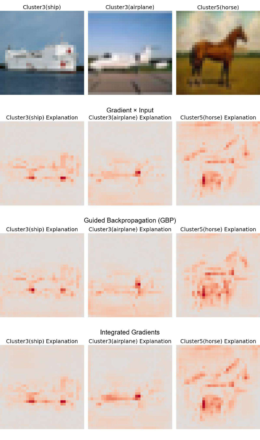
Figure 8: Example of adversarial attack on explanation. The explanation maps of original image can be manipulated to the target explanation.

Appendix B Detailed Hyperparameter

In this section, we provide the detailed hyperparameter for our CIFAR10 dataset in Table 5

Table 5: Comparison of explanation loss for intra-cluster sample and inter-cluster sample on CIFAR10. The results show that our cluster method indeed cluster images with similar explanation.

Models	Learning Rate	$\lambda$
SEP_pos
ConvNet	0.01	5e4
ResNet18	0.001	5e4
Wide ResNet	0.001	5e4
MobileNet	0.01	5e4
SEP_neg
ConvNet	0.01	-3e3
ResNet18	0.001	-1.9e3
Wide ResNet	0.001	-1.9e3
MobileNet	0.01	-1.25e3

Appendix C More experimental results

We list the main results using Gradient X Inputs as training and testing explanation methods for W-ResNet and MobileNetV2 in Table 6.

The detailed values for Transferablity experiments can be found in Table 7 and the detailed values for experiments using TRADES for our method can be found in Table 8.

Table 6: Test results of models trained by Wide ResNet network and MobileNet network on various data sets according to four training methods.The results presented indicate that the performance of models trained using the Wide ResNet network and MobileNet network on different datasets suggests that there is no positive correlation between the model’s interpretability robustness and classification robustness achieved through the SEP_pos and SEP_neg training methods, as compared to the AT training method.

Wide ResNet					MobileNet
MNIST
Method	Expl at start(1e-7)	Expl at end	Clean Acc(%)	Adv Acc	Expl at start	Expl at end	Clean Acc	Adv Acc
Normal	267.050	206.194	99.58	0.00	287.061	188.700	99.08	0.02
AT	842.648	736.839	98.92	82.82	4328.176	3356.135	98.29	94.19
SEP_pos	109.383	99.891	99.01	82.77	319.629	273.256	98.36	94.25
SEP_neg	937.845	744.698	98.87	82.71	8134.157	4454.656	98.33	94.23
FMNIST
Method	Expl at start(1e-7)	Expl at end	Clean Acc(%)	Adv Acc	Expl at start	Expl at end	Clean Acc	Adv Acc
Normal	120.037	69.593	92.79	0.00	180.159	103.941	91.93	0
AT	328.817	257.523	78.10	68.26	4470.448	3571.210	68.72	57.19
SEP_pos	109.996	74.324	77.69	67.79	236.547	172.200	65.11	57.42
SEP_neg	398.006	304.927	78.21	68.05	6032.190	4809.288	66.86	58.16
CIFAR100
Method	Expl at start(1e-7)	Expl at end	Clean Acc(%)	Adv Acc	Expl at start	Expl at end	Clean Acc	Adv Acc
Normal	13.677	5.606	59.13	0	17.015	9.351	43.91	0
AT	30.027	18.389	36.69	16.12	20.054	10.836	21.19	8.64
SEP_pos	22.046	13.704	33.88	13.19	15.234	8.510	21.82	10.05
SEP_neg	31.889	20.045	35.74	15.55	21.544	13.843	21.35	7.88

Table 7: Test results for transferability of explanation robustness. Models are trained with Gradient x Input and tested on different explanation methods.All models are trained on CIFAR10. Even if the interpretation methods during training and testing are different, comparing the training results of our proposed method with the AT training method of the corresponding configuration in Table 2, we can still draw our previous conclusions, which also shows that our conclusions are transferable.

ConvNet			ResNet18
Train:Gradient X Input, Test:Gradient
Method	Expl at start(1e-7)	Expl at end	Expl at start(1e-7)	Expl at end
$SEP_{pos}$	3.054	1.901	9.555	5.903
$SEP_{neg}$	15.093	9.513	55.526	33.176
Train:Gradient X Input, Test:Integrated_Grad
Method	Expl at start(1e-7)	Expl at end	Expl at start	Expl at end
$SEP_{pos}$	3.767	2.404	9.209	6.720
$SEP_{neg}$	17.066	10.923	58.730	38.433

Table 8: The test results of the model trained using the TRADE training method, combined with our approach. The findings indicate that when we apply our method to TRADE, an alternative adversarial training method distinct from MAT, we can still deduce that classification robustness and interpretation robustness are not inherently interconnected.

ConvNet
CIFAR10, TRADE Weight:5
Method	Expl at start(1e-7)	Expl at end	Clean Acc(%)	Adv Acc(%)
TRADE	18.278	11.470	64.5	33.98
TRADE + SEP_pos	3.878	2.285	63.84	33.85
TRADE + SEP_neg	19.781	12.424	64.37	34.07
ConvNet
CIFAR10, TRADE Weight:1
Method	Expl at start(1e-7)	Expl at end	Clean Acc(%)	Adv Acc(%)
TRADE	17.271	10.965	72.63	28.31
TRADE + SEP_pos	4.089	2.296	72.41	28.20
TRADE + SEP_neg	18.504	11.662	72.90	28.34
ResNet18
CIFAR10, TRADE Weight:5
Method	Expl at start(1e-7)	Expl at end	Clean Acc(%)	Adv Acc(%)
TRADE	18.278	11.469	64.50	33.98
TRADE + SEP_pos	12.232	7.527	63.49	34.93
TRADE + SEP_neg	22.571	14.881	63.42	33.30

C.1 More Parameter Sensitivity Studies

Training Epochs We conducted experiments on the ConvNet network using the CIFAR10 dataset to show that our chosen training epoch is reasonable. The results, as presented in Table 9, indicate that the model’s performance undergoes only marginal changes after 25 rounds, despite the epoch count continuing to increase. Choosing 25 epochs does not hurt the reliability of our argument. Besides, the results also support our conclusion. With the increase of training epochs, the classification robustness still increase while the explanation robustness actually decreases.

Table 9: The test results of ConvNet network at different training epochs on the CIFAR10 data set.The findings indicate that as we increase the number of training epochs from 25 , there is only marginal improvement in the model’s performance. Therefore, we have decided to select 25 epochs as the final number of training epochs for all our models. This choice will not impact our final conclusions, while also allowing for faster training speed.

ConvNet, CIFAR10
Training Epoch	Expl at start(1e-7)	Expl at end	Clean Acc(%)	Adv Acc (%)
25	4.388	1.605	64.94	35.25
50	3.885	1.431	65.69	35.94
75	3.671	1.378	66.33	36.27
100	3.557	1.339	66.74	36.50

References

- [1] Christian Szegedy, Wojciech Zaremba, Ilya Sutskever, Joan Bruna, Dumitru Erhan, Ian Goodfellow, and Rob Fergus. Intriguing properties of neural networks. arXiv preprint arXiv:1312.6199, 2013.
- [2] Aleksander Madry, Aleksandar Makelov, Ludwig Schmidt, Dimitris Tsipras, and Adrian Vladu. Towards deep learning models resistant to adversarial attacks. arXiv preprint arXiv:1706.06083, 2017.
- [3] Ann-Kathrin Dombrowski, Maximillian Alber, Christopher Anders, Marcel Ackermann, Klaus-Robert Müller, and Pan Kessel. Explanations can be manipulated and geometry is to blame. Advances in neural information processing systems, 32, 2019.
- [4] Wei Huang, Xingyu Zhao, Gaojie Jin, and Xiaowei Huang. Safari: Versatile and efficient evaluations for robustness of interpretability. In Proceedings of the IEEE/CVF International Conference on Computer Vision, pages 1988–1998, 2023.
- [5] Akhilan Boopathy, Sijia Liu, Gaoyuan Zhang, Cynthia Liu, Pin-Yu Chen, Shiyu Chang, and Luca Daniel. Proper network interpretability helps adversarial robustness in classification. In International Conference on Machine Learning, pages 1014–1023. PMLR, 2020.
- [6] Ian J Goodfellow, Jonathon Shlens, and Christian Szegedy. Explaining and harnessing adversarial examples. arXiv preprint arXiv:1412.6572, 2014.
- [7] David Baehrens, Timon Schroeter, Stefan Harmeling, Motoaki Kawanabe, Katja Hansen, and Klaus-Robert Müller. How to explain individual classification decisions. The Journal of Machine Learning Research, 11:1803–1831, 2010.
- [8] Amirata Ghorbani, Abubakar Abid, and James Zou. Interpretation of neural networks is fragile. In Proceedings of the AAAI conference on artificial intelligence, volume 33, pages 3681–3688, 2019.
- [9] Lin Li and Michael Spratling. Understanding and combating robust overfitting via input loss landscape analysis and regularization. Pattern Recognition, 136:109229, 2023.
- [10] Cihang Xie, Mingxing Tan, Boqing Gong, Alan Yuille, and Quoc V Le. Smooth adversarial training. arXiv preprint arXiv:2006.14536, 2020.
- [11] Hongyang Zhang, Yaodong Yu, Jiantao Jiao, Eric Xing, Laurent El Ghaoui, and Michael Jordan. Theoretically principled trade-off between robustness and accuracy. In International conference on machine learning, pages 7472–7482. PMLR, 2019.
- [12] Nicholas Carlini and David Wagner. Towards evaluating the robustness of neural networks. In 2017 ieee symposium on security and privacy (sp), pages 39–57. Ieee, 2017.
- [13] Nicolas Papernot, Patrick McDaniel, Xi Wu, Somesh Jha, and Ananthram Swami. Distillation as a defense to adversarial perturbations against deep neural networks. In 2016 IEEE symposium on security and privacy (SP), pages 582–597. IEEE, 2016.
- [14] Weilin Xu, David Evans, and Yanjun Qi. Feature squeezing: Detecting adversarial examples in deep neural networks. arXiv preprint arXiv:1704.01155, 2017.
- [15] Ji Lin, Chuang Gan, and Song Han. Defensive quantization: When efficiency meets robustness. arXiv preprint arXiv:1904.08444, 2019.
- [16] Yang Song, Taesup Kim, Sebastian Nowozin, Stefano Ermon, and Nate Kushman. Pixeldefend: Leveraging generative models to understand and defend against adversarial examples. arXiv preprint arXiv:1710.10766, 2017.
- [17] Nicholas Carlini, Florian Tramer, Krishnamurthy Dj Dvijotham, Leslie Rice, Mingjie Sun, and J Zico Kolter. (certified!!) adversarial robustness for free! arXiv preprint arXiv:2206.10550, 2022.
- [18] Anish Athalye, Nicholas Carlini, and David Wagner. Obfuscated gradients give a false sense of security: Circumventing defenses to adversarial examples. In International conference on machine learning, pages 274–283. PMLR, 2018.
- [19] Wieland Brendel, Jonas Rauber, Alexey Kurakin, Nicolas Papernot, Behar Veliqi, Sharada P Mohanty, Florian Laurent, Marcel Salathé, Matthias Bethge, Yaodong Yu, et al. Adversarial vision challenge. In The NeurIPS’18 Competition: From Machine Learning to Intelligent Conversations, pages 129–153. Springer, 2020.
- [20] Dan Hendrycks, Kimin Lee, and Mantas Mazeika. Using pre-training can improve model robustness and uncertainty. In International conference on machine learning, pages 2712–2721. PMLR, 2019.
- [21] Yair Carmon, Aditi Raghunathan, Ludwig Schmidt, John C Duchi, and Percy S Liang. Unlabeled data improves adversarial robustness. Advances in neural information processing systems, 32, 2019.
- [22] Zekai Wang, Tianyu Pang, Chao Du, Min Lin, Weiwei Liu, and Shuicheng Yan. Better diffusion models further improve adversarial training. arXiv preprint arXiv:2302.04638, 2023.
- [23] Tianyu Pang, Kun Xu, Yinpeng Dong, Chao Du, Ning Chen, and Jun Zhu. Rethinking softmax cross-entropy loss for adversarial robustness. arXiv preprint arXiv:1905.10626, 2019.
- [24] Kejiang Chen, Yuefeng Chen, Hang Zhou, Xiaofeng Mao, Yuhong Li, Yuan He, Hui Xue, Weiming Zhang, and Nenghai Yu. Self-supervised adversarial training. In ICASSP 2020-2020 IEEE International Conference on Acoustics, Speech and Signal Processing (ICASSP), pages 2218–2222. IEEE, 2020.
- [25] Florian Tramèr, Alexey Kurakin, Nicolas Papernot, Ian Goodfellow, Dan Boneh, and Patrick McDaniel. Ensemble adversarial training: Attacks and defenses. arXiv preprint arXiv:1705.07204, 2017.
- [26] Tianlong Chen, Zhenyu Zhang, Sijia Liu, Shiyu Chang, and Zhangyang Wang. Robust overfitting may be mitigated by properly learned smoothening. In International Conference on Learning Representations, 2020.
- [27] Gaojie Jin, Xinping Yi, Dengyu Wu, Ronghui Mu, and Xiaowei Huang. Randomized adversarial training via taylor expansion. In Proceedings of the IEEE/CVF Conference on Computer Vision and Pattern Recognition, pages 16447–16457, 2023.
- [28] Dongxian Wu, Shu-Tao Xia, and Yisen Wang. Adversarial weight perturbation helps robust generalization. Advances in Neural Information Processing Systems, 33:2958–2969, 2020.
- [29] Ali Shafahi, Mahyar Najibi, Mohammad Amin Ghiasi, Zheng Xu, John Dickerson, Christoph Studer, Larry S Davis, Gavin Taylor, and Tom Goldstein. Adversarial training for free! Advances in Neural Information Processing Systems, 32, 2019.
- [30] Guanxiong Liu, Issa Khalil, and Abdallah Khreishah. Using single-step adversarial training to defend iterative adversarial examples. In Proceedings of the Eleventh ACM Conference on Data and Application Security and Privacy, pages 17–27, 2021.
- [31] Karen Simonyan, Andrea Vedaldi, and Andrew Zisserman. Deep inside convolutional networks: Visualising image classification models and saliency maps. arXiv preprint arXiv:1312.6034, 2013.
- [32] Avanti Shrikumar, Peyton Greenside, and Anshul Kundaje. Learning important features through propagating activation differences. In International conference on machine learning, pages 3145–3153. PMLR, 2017.
- [33] Sebastian Bach, Alexander Binder, Grégoire Montavon, Frederick Klauschen, Klaus-Robert Müller, and Wojciech Samek. On pixel-wise explanations for non-linear classifier decisions by layer-wise relevance propagation. PloS one, 10(7):e0130140, 2015.
- [34] Ramprasaath R Selvaraju, Abhishek Das, Ramakrishna Vedantam, Michael Cogswell, Devi Parikh, and Dhruv Batra. Grad-cam: Why did you say that? arXiv preprint arXiv:1611.07450, 2016.
- [35] Juyeon Heo, Sunghwan Joo, and Taesup Moon. Fooling neural network interpretations via adversarial model manipulation. Advances in neural information processing systems, 32, 2019.
- [36] Dylan Slack, Sophie Hilgard, Emily Jia, Sameer Singh, and Himabindu Lakkaraju. Fooling lime and shap: Adversarial attacks on post hoc explanation methods. In Proceedings of the AAAI/ACM Conference on AI, Ethics, and Society, pages 180–186, 2020.
- [37] Snir Vitrack Tamam, Raz Lapid, and Moshe Sipper. Foiling explanations in deep neural networks. arXiv preprint arXiv:2211.14860, 2022.
- [38] Xinyang Zhang, Ningfei Wang, Hua Shen, Shouling Ji, Xiapu Luo, and Ting Wang. Interpretable deep learning under fire. In 29th USENIX Security Symposium (USENIX Security 20), 2020.
- [39] Matthew Wicker, Juyeon Heo, Luca Costabello, and Adrian Weller. Robust explanation constraints for neural networks. arXiv preprint arXiv:2212.08507, 2022.
- [40] David Alvarez-Melis and Tommi S Jaakkola. On the robustness of interpretability methods. arXiv preprint arXiv:1806.08049, 2018.
- [41] Jiefeng Chen, Xi Wu, Vaibhav Rastogi, Yingyu Liang, and Somesh Jha. Robust attribution regularization. Advances in Neural Information Processing Systems, 32, 2019.
- [42] Ruixiang Tang, Ninghao Liu, Fan Yang, Na Zou, and Xia Hu. Defense against explanation manipulation. Frontiers in big Data, 5:704203, 2022.
- [43] Karen Simonyan, Andrea Vedaldi, and Andrew Zisserman. Deep inside convolutional networks: Visualising image classification models and saliency maps. arxiv 2013. arXiv preprint arXiv:1312.6034, 2019.
- [44] Zifan Wang, Matt Fredrikson, and Anupam Datta. Robust models are more interpretable because attributions look normal. arXiv preprint arXiv:2103.11257, 2021.
- [45] Francesco Croce and Matthias Hein. Reliable evaluation of adversarial robustness with an ensemble of diverse parameter-free attacks. In International conference on machine learning, pages 2206–2216. PMLR, 2020.
- [46] Alex Krizhevsky, Geoffrey Hinton, et al. Learning multiple layers of features from tiny images. 2009.
- [47] Kaiming He, Xiangyu Zhang, Shaoqing Ren, and Jian Sun. Deep residual learning for image recognition. In Proceedings of the IEEE conference on computer vision and pattern recognition, pages 770–778, 2016.
- [48] Stuart Lloyd. Least squares quantization in pcm. IEEE transactions on information theory, 28(2):129–137, 1982.
- [49] Yann LeCun, Bernhard Boser, John S Denker, Donnie Henderson, Richard E Howard, Wayne Hubbard, and Lawrence D Jackel. Backpropagation applied to handwritten zip code recognition. Neural computation, 1(4):541–551, 1989.
- [50] Han Xiao, Kashif Rasul, and Roland Vollgraf. Fashion-mnist: a novel image dataset for benchmarking machine learning algorithms. arXiv preprint arXiv:1708.07747, 2017.
- [51] Ya Le and Xuan Yang. Tiny imagenet visual recognition challenge. CS 231N, 7(7):3, 2015.
- [52] Sergey Zagoruyko and Nikos Komodakis. Wide residual networks. arXiv preprint arXiv:1605.07146, 2016.
- [53] Andrew G Howard, Menglong Zhu, Bo Chen, Dmitry Kalenichenko, Weijun Wang, Tobias Weyand, Marco Andreetto, and Hartwig Adam. Mobilenets: Efficient convolutional neural networks for mobile vision applications. arXiv preprint arXiv:1704.04861, 2017.
- [54] Mark Sandler, Andrew Howard, Menglong Zhu, Andrey Zhmoginov, and Liang-Chieh Chen. Mobilenetv2: Inverted residuals and linear bottlenecks. In Proceedings of the IEEE conference on computer vision and pattern recognition, pages 4510–4520, 2018.
- [55] Spyros Gidaris and Nikos Komodakis. Dynamic few-shot visual learning without forgetting. In Proceedings of the IEEE conference on computer vision and pattern recognition, pages 4367–4375, 2018.
- [56] Hao Zheng, Zhanlei Yang, Wenju Liu, Jizhong Liang, and Yanpeng Li. Improving deep neural networks using softplus units. In 2015 International joint conference on neural networks (IJCNN), pages 1–4. IEEE, 2015.
- [57] Jost Tobias Springenberg, Alexey Dosovitskiy, Thomas Brox, and Martin Riedmiller. Striving for simplicity: The all convolutional net. arXiv preprint arXiv:1412.6806, 2014.
- [58] Diederik P Kingma and Jimmy Ba. Adam: A method for stochastic optimization. arXiv preprint arXiv:1412.6980, 2014.
- [59] Tianyu Pang, Xiao Yang, Yinpeng Dong, Hang Su, and Jun Zhu. Bag of tricks for adversarial training. arXiv preprint arXiv:2010.00467, 2020.