Locally regular and efficient tests in non-regular semiparametric models

Abstract

This paper considers hypothesis testing in semiparametric models which may be non-regular. I show that C($\alpha$) style tests are locally regular under mild conditions, including in cases where locally regular estimators do not exist, such as models which are (semiparametrically) weakly identified. I characterise the appropriate limit experiment in which to study local (asymptotic) optimality of tests in the non-regular case, permitting the generalisation of classical power bounds to this case. I give conditions under which these power bounds are attained by the proposed C($\alpha$) style tests. The application of the theory to a single index model and an instrumental variables model is worked out in detail.

JEL classification: C10, C12, C14, C21, C39

Keywords: Hypothesis testing, local asymptotics, uniformity, semiparametric models, weak identification, boundary, regularisation, single-index, instrumental variables.

Abstract

This Supplementary Material contains the following sections:

• Details on notation

• Additional results

• Additional details and proofs for the examples

• Additional simulation details & results

• Tables and Figures

1 Introduction

It is often considered desirable that estimators are “locally regular” in that they exhibit the same limiting behaviour under the true parameter as they do under sequences of “local alternatives” which cannot be consistently distinguished from the true parameter, even asymptotically.

Unfortunately, there are many semiparametric models in which locally regular estimators do not exist. One necessary condition is given by Chamberlain (1986), who shows that if the efficient information for a scalar parameter is 0, then no locally regular estimator of that parameter exists. This result can be extended to singularity of the efficient information matrix implying the non-existence of locally regular estimators of Euclidean parameters. Models in which this may occur are called “non-regular”; many widely used models in econometrics are non-regular (for certain parameter values). Prominent examples include instrumental variables models, discrete choice models, single index models, mixed proportional hazard models, sample selection models and error-in-variables models.

In this paper, I demonstrate that locally regular tests exist in a broad class of non-regular models, despite the non-existence of locally regular estimators. In particular, I show that a class of tests based on the C$(\alpha)$ idea of Neyman (1959, 1979) are locally regular, i.e. they exhibit the same limiting behaviour under both the true parameter and local alternatives.

These tests are based on a quadratic form of moment conditions evaluated under the null hypothesis. The key [C($\alpha$)] idea which ensures the local regularity is that the moment conditions must be (asymptotically) orthogonal to the collection of score functions for all nuisance parameters. Such moment conditions always exist and can be constructed from any initial choice of moment conditions via an orthogonal projection.

A key advantage of these C($\alpha$) tests is that they do not (asymptotically) overreject under (semiparametric) weak identification asymptotics: such asymptotics consider the limiting behaviour under local alternatives to the true parameter. The local regularity of these tests ensures that if the test is asymptotically of level $\alpha$ under any fixed parameter consistent with the null, it is also asymptotically of level $\alpha$ under any sequence of local alternatives consistent with the null, i.e. under weak identification asymptotics. In addition to the well-studied case where weak identification is due to potential identification failure at certain values of a finite dimensional nuisance parameter, the results in this paper also apply to the case where identification failure is due to the value of infinite dimensional parameters.

Achieving this local regularity does not come at the expense of (local asymptotic) power. I characterise (local asymptotic) power bounds for tests in non-regular models and show that the C($\alpha$) tests proposed in this paper acheive these power bounds provided the moment conditions are chosen appropriately. These power bounds contain those for regular models as a special case and the imposed conditions are weaker than those in the literature.

Following the theoretical development, I provide fully worked out details for two examples: (i) a single index model which may be weakly identified when the link function is too flat and (ii) an instrumental variables model which may be weakly identified when the (nonparametric) first stage is too close to the zero function. Simulation experiments based on these examples demonstrate that the proposed tests display good finite sample performance.

This paper is connected to three main strands of the literature: the first is that concerned with general results on estimation and testing in semiparametric models. Much of this is now textbook material: see e.g. Newey (1990); Choi et al. (1996); Bickel et al. (1998); van der Vaart (1998, 2002). The second is the literature on C($\alpha$) style tests. Such tests were introduced by Neyman (1959, 1979) and have seen many useful applications, most recently as a way to handle machine learning or otherwise high dimensional first steps (see e.g. Chernozhukov et al., 2015; Bravo et al., 2020; Chernozhukov et al., 2022). In this paper, the structure which ensures the good performance of these tests in such settings is used for a different purpose – to create tests which remain robust in non-regular settings. Lastly, the literature on robust testing in non – regular or otherwise non – standard settings is closely related to this paper (e.g. Andrews and Guggenberger, 2009; Romano and Shaikh, 2012; Elliott et al., 2015; McCloskey, 2017). In particular, the locally regular tests derived in this paper are particularly useful in cases of weak identification and therefore this paper is closely related to the literature on weak identification robust inference in econometrics (e.g. Staiger and Stock, 1997; Dufour, 1997; Stock and Wright, 2000; Kleibergen, 2005; Andrews and Cheng, 2012; Andrews and Mikusheva, 2015, 2016). In particular this paper is most closely related to the recent work on semiparametric weak identification (Kaji, 2021; Andrews and Mikusheva, 2022) and extends the notion of semiparametric weak identification considered there to non – i.i.d. models.

2 Locally regular testing

The goal considered throughout this paper is to construct hypothesis tests of the form $H_{0}:\theta=\theta_{0}$ against $H_{1}:\theta\neq\theta_{0}$ in the sequence of models $\mathcal{P}_{n}=\{P_{n,\gamma}:\gamma\in\Gamma\}$ where $\gamma=(\theta,\eta)\in\Gamma=\Theta\times\mathcal{H}$ for some open $\Theta\subset\mathbb{R}^{d_{\theta}}$ and $\mathcal{H}$ an arbitrary set. Each $\mathcal{P}_{n}$ consists of probability measures on a measurable space $(\mathcal{W}_{n},\mathcal{B}(\mathcal{W}_{n}))$ and is dominated by a $\sigma$-finite measure $\nu_{n}$.

In this section I will define local regularity for testing and heuristically describe how such tests can be constructed, with technical details deferred until the following section. I then explain how this concept can be useful to derive robust testing procedures in two common non-standard inference problems.

2.1 Defining local regularity for tests

Local regularity for estimators

To motivate the definition of local regularity for tests, I first recall the definition of local regularity of estimators. Suppose that $\hat{\theta}_{n}$ is a sequence of estimators of $\theta$ and $P_{n,\gamma,h}=P_{n,(\theta+\tau/\sqrt{n},\eta_{n}(b))}$ a sequence of local alternatives to $P_{n,\gamma}$ for some $h=(\tau,b)\in H\coloneqq\mathbb{R}^{d_{\theta}}\times B$. The estimator sequence $\hat{\theta}_{n}$ is then called “locally regular” at $\gamma$ if

$$\sqrt{n}\left(\hat{\theta}_{n}-\theta-\frac{\tau}{\sqrt{n}}\right)\overset{P_{n,\gamma,h}}{\rightsquigarrow}\mathcal{L}_{\gamma},\qquad h\in H.$$ (1)

for some law ${\mathcal{L}}_{\gamma}$ which – as indicated by the notation – may depend on $\gamma$ but not on $h$.

Local regularity for tests

Motivated by (1), I now define a notion of local regularity for tests of $H_{0}$ against $H_{1}$.

Definition 1:

A sequence of tests $\phi_{n}:\mathcal{W}_{n}\to[0,1]$ of the hypothesis $H_{0}:\theta=\theta_{0}$ against $H_{1}:\theta\neq\theta_{0}$ is asymptotically level $\alpha$ and locally regular if

$$\uppi_{n}(\tau,b)\coloneqq P_{n,\gamma,h}\phi_{n}\to\uppi_{\gamma}(\tau),\quad h\in H\quad\text{ and }\quad\uppi_{\gamma}(0)\leq\alpha.$$ (2)

In words, the finite sample (local) power function of the test, $\uppi_{n}$ converges under each $P_{n,\gamma,h}$ to a function $\uppi_{\gamma}$ which depends only on $\tau$. This requirement is in the same spirit as (1): the parameter $b$ which describes local deviations from $\eta$ does not affect the limit. If a sequence of tests does not satisfy (1) I shall call it locally non – regular.

Local regularity of test sequences as in Definition 1 is a pointwise concept. It is also of interest to consider a version of local regularity which holds uniformly over certain subsets.

Definition 2:

A sequence of tests $\phi_{n}:\mathcal{W}_{n}\to[0,1]$ of the hypothesis $H_{0}:\theta=\theta_{0}$ against $H_{1}:\theta\neq\theta_{0}$ is asymptotically level $\alpha$ and locally uniformly regular on $K\subset H$ if (2) holds uniformly on $K$.

$$\sup_{(\tau,b)\in K}|\uppi_{n}(\tau,b)-\uppi_{\gamma}(\tau)|\to 0\quad\text{ and }\quad\uppi_{\gamma}(0)\leq\alpha.$$ (3)

In the case where $H$ is a (pseudo-)metric space and $K$ is a compact set, to go from the pointwise convergence in (2) to the uniform convergence in (3) it is necessary and sufficient to show that the sequence of functions $\uppi_{n}$ is asymptotically equicontinuous on $K$.

Directly establishing asymptotic equicontinuity of the power functions $\uppi_{n}(\tau,b)$ may be complicated in many cases. It is, however, often possible to show stronger results which immediately imply this property. For instance, if one can show that the functions $h\mapsto P_{n,\gamma,h}$ are asymptotically equicontinuous in total variation, the required asymptotic equicontinuity of the power functions follows immediately. Despite being (much) stronger, this requirement can often be relatively straightforward to demonstrate. For example, in the classical case of a parametric model for i.i.d. data, this asymptotic equicontinuity in total variation follows from the differentiability in quadratic mean condition typically used to demonstrate local asymptotic normality (cf. e.g. Theorem 7.2 in van der Vaart (1998) and Theorem 80.13 in Strasser (1985)).

A class of locally regular tests

To construct tests of $H_{0}:\theta=\theta_{0}$ against $H_{1}:\theta\neq\theta_{0}$ which have property (2) (or (3)), I use a generalisation of the class of C($\alpha$) tests introduced by Neyman (1959, 1979) to characterise optimal tests in regular parametric models.

I will heuristically outline the construction of C($\alpha$) tests in such parametric models to build intuition for the theoretical development in the following section. Thus, suppose temporarily that $\mathcal{H}\subset\mathbb{R}^{d_{\eta}}$ and the observed data $(W_{1},\ldots,W_{n})$ is drawn i.i.d. from a parametric density $p_{\gamma}$. Let $\dot{\nu}_{\gamma}$ be the score functions for the (now finite dimensional) nuisance parameter $\eta$, i.e. the partial derivatives of the log likelihood for an observation $W$: $\dot{\nu}_{\gamma}\coloneqq\nabla_{\eta}\log p_{\gamma}$. Let $f_{\gamma}=f_{\theta,\eta}$ be a vector of $d_{\theta}$ moment conditions which are mean-zero under the null hypothesis, i.e. $\mathbb{E}_{\theta_{0},\eta}f_{\theta_{0},\eta}(W)=0$.

Such regular parametric models are typically locally asymptotically normal (“LAN”): the log-likelihood ratio admits a local quadratic approximation:

$$\log\frac{q_{\gamma,h}}{p_{\theta,\eta}}=\frac{1}{\sqrt{n}}\sum_{i=1}^{n}\tau^{\prime}\dot{\ell}_{\gamma}(W_{i})+b^{\prime}\dot{\nu}_{\gamma}(W_{i})-\mathbb{E}_{\gamma}\left[\tau^{\prime}\dot{\ell}_{\gamma}(W_{i})+b^{\prime}\dot{\nu}_{\gamma}(W_{i})\right]^{2}+o_{P_{\gamma}}(1),$$ (4)

for $q_{\gamma,h}\coloneqq p_{\theta+\tau/\sqrt{n},\eta+b/\sqrt{n}}$ where $(\tau,b)\in\mathbb{R}^{d_{\theta}+d_{\eta}}$ and $\dot{\ell}_{\gamma}$ the score functions for $\theta$: $\dot{\ell}_{\gamma}\coloneqq\nabla_{\theta}\log p_{\gamma}$.

Under LAN, the asymptotic distribution of scaled sums of the moment condition $f_{\gamma}$ under the local alternative $(\theta+\tau/\sqrt{n},\eta+b/\sqrt{n})$ is given by Le Cam’s third Lemma (e.g. van der Vaart, 1998, Example 6.5):

$$\frac{1}{\sqrt{n}}\sum_{i=1}^{n}f_{\gamma}(W_{i})\overset{P_{n,\gamma,h}}{\rightsquigarrow}\mathcal{N}\left(\mathbb{E}_{\gamma}[f_{\gamma}(W)\dot{\ell}_{\gamma}(W)^{\prime}]\tau+\mathbb{E}[f_{\gamma}(W)\dot{\nu}_{\gamma}(W)^{\prime}]b,\ \mathbb{E}_{\gamma}[f_{\gamma}(W)f_{\gamma}(W)^{\prime}]\right).$$

In consequence, the limiting distribution will depend on $b$ if and only if $\mathbb{E}[f_{\gamma}(W)\dot{v}_{\gamma}(W)]\neq 0$.

In order to ensure this covariance is zero, a C($\alpha$) test is not based on the original moment condition $f_{\gamma}$, but rather on the orthogonal projection

$$g_{\gamma}\coloneqq f_{\gamma}-\mathbb{E}_{\gamma}\left[f_{\gamma}(W)\dot{\nu}_{\gamma}(W)^{\prime}\right]\mathbb{E}_{\gamma}\left[\dot{\nu}(W)\dot{\nu}_{\gamma}(W)^{\prime}\right]^{-1}\dot{\nu}_{\gamma}=\Pi\left[f_{\gamma}\middle|\operatorname{Span}(\dot{\nu}_{\gamma})^{\perp}\right],$$ (5)

where $\Pi[\cdot|\mathcal{S}]$ is the orthogonal projection onto the closed subspace $\mathcal{S}\subset L_{2}(P_{\gamma})$. Then, as $\mathbb{E}[g_{\gamma}(W)\dot{\nu}_{\gamma}(W)^{\prime}]=0$ by construction, by the same argument as above

$$\frac{1}{\sqrt{n}}\sum_{i=1}^{n}g_{\gamma}(W_{i})\overset{P_{n,\gamma,h}}{\rightsquigarrow}\mathcal{N}\left(\mathbb{E}_{\gamma}[g_{\gamma}(W)\dot{\ell}_{\gamma}(W)^{\prime}]\tau,\ \mathbb{E}_{\gamma}[g_{\gamma}(W)g_{\gamma}(W)^{\prime}]\right).$$ (6)

In practice, for the test to be feasible one must replace the unknown nuisance parameters $\eta$ with an estimator (which may be estimated under the null). Typically one also estimates the (pseudo-)inverse of $V_{\gamma}\coloneqq\mathbb{E}_{\gamma}[g_{\gamma}(W)g_{\gamma}(W)^{\prime}]$ and weights the estimated components $\frac{1}{\sqrt{n}}\sum_{i=1}^{n}\hat{g}_{n,\theta}(W_{i})$ by this matrix in a quadratic form, forming a feasible test statistic $\hat{S}_{n,\theta}$. Provided these estimators are sufficiently accurate, $\hat{S}_{n,\theta}$ will converge to a $\chi^{2}$ distribution under $P_{n,\gamma,h}$. As such score – type test statistics based on the moment conditions $g_{\gamma}$ will have asymptotic distributions free of $b$. One can then choose an appropriate critical value $c$ such that the test of the form $\bm{1}\{\hat{S}_{n,\theta}>c\}$ does not over-reject under any $P_{n,\gamma,h}$ consistent with $H_{0}$.

Tests constructed in this manner will be locally regular tests in the sense of definition 1. The (rigorous) extension of this argument to the semiparametric case, with possible singularity of the variance matrix $V_{\gamma}$ (as may happen, for example, in cases with potential identification failure or in underidentified models) is given in Section 3.

The non-iid case

The heuristic derivation of the class of C($\alpha$) tests given above imposed that the researcher observed a random sample, i.e. that the model $\mathcal{P}_{n}$ consists of $n$-fold product measures $P_{n,\gamma}\coloneqq P_{\gamma}^{n}$. This is not necessary for the local regularity of C($\alpha$) tests, and is not imposed in the general theory discussed in Section 3. It does, however, routinely simplify expressions and the demonstration of the required regularity conditions. Given this and its central role as a benchmark case in statistics and econometrics, the simplifications available in the i.i.d. case are explicitly discussed in Section 3.4.

Power optimality

As noted above, Neyman (1959, 1979) initially developed the C($\alpha$) test in order to discuss testing optimality. In regular parametric models, the conclusion is (up to regularity conditions) that C($\alpha$) tests based on $\dot{\ell}_{\gamma}$, the scores for $\theta$, attain the (local asymptotic) power bounds for various classes of testing problems. This is known to also be true in (regular) semiparametric models if (a) the data is i.i.d. (cf. Chapter 25 in van der Vaart, 1998) or (b) the information operator (as defined in Choi et al., 1996, p. 846) is boundedly invertible (Choi et al., 1996). In Section 3, I show that this result holds without requiring either (a) or (b) and, moreover, persists in the non – regular case, where the efficient information matrix may be rank deficient.

2.2 Robust testing in non-standard problems

I now explain how the ideas just described can be used to derive tests which are well behaved in the face of two commonly encountered non-standard inference problems in econometrics. I provide examples in each case, for which locally regular C($\alpha$) style tests will be explicitly developed in Section 4.

Weak identification

As noted in the introduction, in many models there are values of $\gamma$ such that estimators satisfying (1) do not exist. Points $\gamma$, where the parameter of interest is un- or under-identified provide an important class of examples. As is well known, even if $\theta$ is identified at $\gamma$, finite sample inference may still be poor if $\gamma$ is too close to a point of identification failure relative to the amount of information contained in the sample. Such weak identification concerns have been widely studied in models where the part of $\eta$ which causes the potential identification failure is finite dimensional (e.g. Andrews and Cheng, 2012; Andrews and Mikusheva, 2015). There are also many examples where this may occur due to the value of infinite-dimensional nuisance parameters. Kaji (2021) considers estimation in weakly identified semiparametric models, whilst Andrews and Mikusheva (2022) consider semiparametric weak identification in GMM models. Both use a differentiability in quadratic mean (DQM) condition to define “weak identification embeddings” in i.i.d. models. As such DQM - type conditions are less straightforward to work with in non - i.i.d. cases, in this paper I use an analogous notion – based directly on the LAN expansion – which broadens the applicability of this class of semiparametric weak identification sequences. The key property of these sequences is that they are local (i.e. contiguous) alternatives to a point of identification failure.

I now give three examples of semiparametric models where the parameter of interest $\theta$ may be un- or under- identified depending on the value of an infinite dimensional nuisance parameter.

Example 1 (Single – index model):

Suppose that the researcher observes $n$ i.i.d. copies of $W=(Y,X)$ where

$$Y=f(X_{1}+X_{2}^{\prime}\theta)+\epsilon,\qquad\mathbb{E}[\epsilon|X]=0,$$

and where $f$ belongs to some set of continuously differentiable functions $\mathscr{F}$. The description of the model is completed by a parameter $\zeta$ which describes the distribution of $(X,\epsilon)$. If $f$ is flat, i.e. $f^{\prime}=0$, then the parameter $\theta$ is unidentified.

Example 2 (Instrumental variables):

Suppose the researcher observes $n$ i.i.d. copies of $W=(Y,X,Z)$ where

$$Y=X^{\prime}\theta+Z_{1}^{\prime}\beta+\epsilon,\qquad\mathbb{E}[\epsilon|Z]=0,\qquad Z=(Z_{1}^{\prime},Z_{2}^{\prime})^{\prime}.$$

If the $k$-th component of $\pi(Z)\coloneqq\mathbb{E}[X|Z]$ is zero, $\theta_{k}$ is unidentified.

Example 3 (Independent components supply & demand model):

Suppose the researcher observes $n$ i.i.d. copies of $W=Y\in\mathbb{R}^{2}$, where

$$Y=A(\theta,\sigma)^{-1}\epsilon,\qquad\mathbb{E}\epsilon=0,\quad\mathrm{Var}(\epsilon)=I,\quad\epsilon_{1}\mathchoice{\mathrel{\hbox to0.0pt{$\displaystyle\perp$\hss}\mkern 2.0mu{\displaystyle\perp}}}{\mathrel{\hbox to0.0pt{$\textstyle\perp$\hss}\mkern 2.0mu{\textstyle\perp}}}{\mathrel{\hbox to0.0pt{$\scriptstyle\perp$\hss}\mkern 2.0mu{\scriptstyle\perp}}}{\mathrel{\hbox to0.0pt{$\scriptscriptstyle\perp$\hss}\mkern 2.0mu{\scriptscriptstyle\perp}}}\epsilon_{2},$$

with

$$A(\theta,\sigma)=\begin{bmatrix}\sigma_{1}^{-1}&0\\ 0&\sigma_{2}^{-1}\end{bmatrix}\begin{bmatrix}1&-\theta_{1}\\ 1&-\theta_{2}\end{bmatrix},\quad\sigma\in(0,\infty)^{2},\quad\theta\in(-\infty,0)\times(0,\infty).$$

This simple equilibrium supply & demand model is completed by the density functions $\zeta_{1},\zeta_{2}$ of $\epsilon_{1},\epsilon_{2}$ respectively. If no more than one $\epsilon_{k}$ has a standard Gaussian distribution, $\theta$ is identified (Comon, 1994). If $\epsilon\sim\mathcal{N}(0,I)$, $\theta$ is underidentified.

In each of the above examples, no locally regular estimator exists. For Examples 1 and 2, locally regular C($\alpha$) tests which satisfy $\uppi(0)\leq\alpha$ are developed in Section 4. The local regularity of these tests ensures that they do not asymptotically over-reject under semiparametric weak identification parameter sequences. The simulation exercises reported in the same section demonstrate that this approximation provides a good guide to the finite sample reality: unlike many alternative procedures, these tests exhibit finite sample rejection frequencies close to the nominal level under the null, even in very weakly identified settings.

Each of these examples are in the i.i.d. case, though as emphasised above, this is not a requirement. For example, locally regular C($\alpha$) tests for the potentially un- / under- identified parameter in a structural vector autoregressive model built on top of an ICA model similar to Example 3 were developed in Hoesch et al. (2024a).

Parameters close to the boundary

A second non-standard inference problem which has attracted substantial attention in statistics & econometrics is inference when a finite - dimensional nuisance parameters may be at, or close to, the boundary. See, amongst others, Geyer (1994); Andrews (1999, 2001); Ketz (2018).

In this scenario, as explained in detail in the aforementioned papers, the limiting distributions of extremum estimators are non-normal when true parameter is at the boundary of the parameter space. In otherwise regular models, the same true when the true parameter is “close” to this boundary, i.e. along local (contiguous) alternatives to such a boundary point, by virtue of Le Cam’s third lemma (e.g. van der Vaart, 1998, Theorem 6.6).

In consequence, using the “standard” normal approximations which usually obtain for extremum estimators (cf. Newey and McFadden, 1994) can lead to either misleading inference or poor power. In the literature there are examples of boundary problems where “standard” tests over-reject (e.g. Andrews and Guggenberger, 2010) as well as examples where they are conservative and exhibit poor power (e.g. Ketz, 2018).

Under regularity conditions, boundary - constrained estimators of the nuisance parameters typically remain $\sqrt{n}$ - consistent (albeit not asymptotically normal). Due to the orthogonalisation (5), plugging in any $\sqrt{n}$ - consistent estimator $\hat{\eta}_{n}$ of $\eta$ is sufficient to ensure that the resulting feasible moment function (i.e. $\hat{g}_{n,\theta}=g_{\theta,\hat{\eta}_{n}}$) achieves the same normal limit as in (6).

In the semiparametric setting a natural generalisation of this boundary - constrained phenomenon is that of inference when nuisance functions are estimated under shape restrictions which may be close to binding. Consider the following example, based on the single index model of Example 1.

Example 4:

Recall the model of Example 1:

$$Y=f(X_{1}+X_{2}^{\prime}\theta)+\epsilon,\qquad\mathbb{E}[\epsilon|X]=0,$$

and now suppose that $f$ belongs to some subset of continuously differentiable functions $\mathscr{F}$ which also satisfy a shape restriction. For instance, $\mathscr{F}$ may contain only monotonically increasing functions or convex functions.

Analogously to in the parametric case, plugging in nuisance functions estimated under shape constraints causes no problems for C$(\alpha)$ style tests, which retain the same asymptotic distribution whether or not the constraints are (close to) binding.

In the simulation study of Section 4, this phenomenon is explored in the context of Example 4. The locally regular C($\alpha$) test with $f$ estimated under a monotonicity restriction demonstrates good performance, including when the imposed restriction is close to binding. In contrast, a Wald test based on a non-linear least squares estimator (as in Ichimura (1993)) delivers conservative inference when such a restricted estimator of $f$ is used.

3 Main results

This section establishes the main theoretical results of the paper. These are first established under high-level assumptions, which allows the results to be stated in a manner which applies to many situations, including cases with dependent or non-identically distributed data. Section 3.4 considers simplifications which are valid in the benchmark case of i.i.d. data and a “smooth” statistical model.

3.1 The setting

Local asymptotic normality

I now formalise and generalise the required LAN condition as in (4). Let $H_{\gamma}=\mathbb{R}^{d_{\theta}}\times B_{\gamma}$ be a subset of a linear space containing 0, and suppose that $\{P_{n,\gamma,h}:h\in H_{\gamma}\}\subset\mathcal{P}_{n}$ are such that $P_{n,\gamma}=P_{n,\gamma,0}$. A typical element of $H_{\gamma}$ will be written as $h=(\tau,b)\in\mathbb{R}^{d_{\theta}}\times B_{\gamma}$. The measures $P_{n,\gamma,h}$ should be interpreted as local perturbations of the measure $P_{n,\gamma}$ in a direction $h\in H_{\gamma}$.

The null hypothesis $H_{0}:\theta=\theta_{0}$ corresponds to the set of perturbations $H_{\gamma,0}\coloneqq\{(0,b):b\in B_{\gamma}\}$ and the alternative $H_{1}:\theta\neq\theta_{0}$ to $H_{\gamma,1}\coloneqq\{h=(\tau,b):0\neq\tau\in\mathbb{R}^{d_{\theta}},b\in B_{\gamma}\}$. As such, $P_{n,\gamma,h}$ for $h\in H_{\gamma,0}$ will be referred to as local perturbations consistent with the null hypothesis, whilst $P_{n,\gamma,h}$ for $h\in H_{\gamma,1}$ are local alternatives. To frame this another way, I consider tests of $\tau=0$ against $\tau\neq 0$ in the local models $\{P_{n,\gamma,h}:h\in H_{\gamma}\}$.

The key technical condition under which the theory in this paper is developed is local asymptotic normality (see e.g. van der Vaart, 1998, Chapter 7 or Le Cam and Yang, 2000, Chapter 6). Define the log-likelihood ratios

$$L_{n,\gamma}(h)\coloneqq\log\frac{p_{n,\gamma,h}}{p_{n,\gamma,0}},\qquad\text{ where }\ p_{n,\gamma,h}\coloneqq\frac{\mathrm{d}P_{n,\gamma,h}}{\mathrm{d}\nu_{n}},\text{ for }h\in H_{\gamma}.$$ (7)

Assumption 1 (Local asymptotic normality):

$L_{n,\gamma}(h)$ satisfies

$$L_{n,\gamma}(h)=\Delta_{n,\gamma}h-\frac{1}{2}\|\Delta_{n,\gamma}h\|^{2}+R_{n,\gamma}(h),$$ (8)

where $h=(\tau,b)$, $\Delta_{n,\gamma}:\overline{\operatorname{lin}}\ H_{\gamma}\to L_{2}^{0}(P_{n,\gamma})$ are bounded linear maps and for all $h$ in $H_{\gamma}$, $R_{n,\gamma}(h)\xrightarrow{P_{n,\gamma}}0$. Additionally, suppose that for each $h$ in $H_{\gamma}$, $(\Delta_{n,\gamma}h)_{n\in\mathbb{N}}$ is uniformly square $P_{n,\gamma}$-integrable and

$$\Delta_{n,\gamma}h\overset{P_{n,\gamma}}{\rightsquigarrow}\mathcal{N}(0,\sigma_{\gamma}(h)),\qquad\sigma_{\gamma}(h)\coloneqq\lim_{n\to\infty}\|\Delta_{n,\gamma}h\|^{2}.$$

$\Delta_{n,\gamma}$ is the score operator (cf. van der Vaart, 1998, p. 371). It produces score functions (or “scores”) from “directions” $h\in H_{\gamma}$. As such, the LAN expansion (8) requires that the log-likelihoods are approximately equal to the score less half of its variance. This approximation and the asymptotic normality of the scores leads to contiguity.

Remark 1:

Assumption 1 ensures that the sequences $(P_{n,\gamma})_{n\in\mathbb{N}}$ and $(P_{n,\gamma,h})_{n\in\mathbb{N}}$ are mutually contiguous for any $h\in H_{\gamma}$ (see e.g. van der Vaart, 1998, Example 6.5).

Remark 2:

If $H_{\gamma}$ is (pseudo-)metrised one may consider a uniform version of Assumption 1, i.e. uniform local asymptotic normality. Such a version is given in Assumption S1 and – as shown by Proposition S2 – is equivalent to Assumption 1 plus asymptotic equicontinuity on compact sets of $h\mapsto\Delta_{n,\gamma}h$ (in $L_{2}(P_{n,\gamma})$) and $h\mapsto P_{n,\gamma,h}$ (in total variation). The latter equicontinuity condition, in particular, is of interest regarding local uniform regularity and hence local uniformity of size control; cf. Corollaries 3, 4 and Lemma 1 below.

In the case where the index $n$ corresponds to an increasing sample of i.i.d. data, LAN is satisfied under a pathwise differentiability in quadratic mean condition (e.g. van der Vaart, 1998, Lemma 25.14); this situation will be discussed further in Section 3.4. Whilst LAN is particularly straightforward to establish in this “smooth i.i.d.” case, it also holds in other settings and sufficient conditions for LAN applicable to various settings exist in the literature.

C($\alpha$) – style test statistics

The C($\alpha$) – style test statistics proposed in this paper are feasible versions of a quadratic form of $d_{\theta}$-moment conditions $g_{n,\gamma}\in L_{2}(P_{n,\gamma})$. In particular, the statistic will be a quadratic form of estimators of the moment conditions weighted by an estimator of the Moore-Penrose pseudo-inverse of their variance matrix. To derive the limiting distribution of the statistic, I impose a high-level joint convergence requirement on the scores and moment functions.

Assumption 2 (Joint convergence):

For $d_{\theta}$-dimensional moment conditions $g_{n,\gamma}\in L_{2}(P_{n,\gamma})$,

$$\left(\Delta_{n,\gamma}h,\;g_{n,\gamma}^{\prime}\right)^{\prime}\overset{P_{n,\gamma}}{\rightsquigarrow}\mathcal{N}\left(0,\Sigma_{\gamma}(h)\right),\quad\text{for each }h\in H_{\gamma},$$

where, for $h=(\tau,b)$,

$$\Sigma_{\gamma}(h)\coloneqq\begin{bmatrix}\sigma_{\gamma}(h)&\tau^{\prime}\Sigma_{\gamma,21}^{\prime}\\ \Sigma_{\gamma,21}\tau&V_{\gamma}\end{bmatrix}=\lim_{n\to\infty}\begin{bmatrix}\|\Delta_{n,\gamma}h\|^{2}&\left\langle{\Delta_{n,\gamma}(\tau,0)}\,,\,{g_{n,\gamma}^{\prime}}\right\rangle\\ \left\langle{g_{n,\gamma}}\,,\,{\Delta_{n,\gamma}(\tau,0)}\right\rangle&\left\langle{g_{n,\gamma}}\,,\,{g_{n,\gamma}^{\prime}}\right\rangle\end{bmatrix}.$$

Built-in to Assumption 2 is a requirement of asymptotic orthogonality of the moment functions and scores for the nuisance parameters $\eta$. This generalises the explicit orthogonal projection construction discussed around equations (5) – (6).

Remark 3:

For Assumption 2 to hold it is necessary that the $g_{n,\gamma}$ are approximately zero mean: since $(g_{n,\gamma})_{n\in\mathbb{N}}$ is uniformly integrable, $P_{n,\gamma}g_{n,\gamma}=o(1)$. It is also necessary that the $g_{n,\gamma}$ satisfy an approximate orthogonality property with the scores for nuisance parameters. In particular, as $([\Delta_{n,\gamma}h]g_{n,\gamma})_{n\in\mathbb{N}}$ is uniformly integrable for each $h=(\tau,b)\in H_{\gamma}$,

$$\lim_{n\to\infty}\left\langle{\Delta_{n,\gamma}h}\,,\,{g_{n,\gamma}^{\prime}}\right\rangle=\tau^{\prime}\Sigma_{\gamma,21}^{\prime}=\lim_{n\to\infty}\left\langle{\Delta_{n,\gamma}(\tau,0)}\,,\,{g_{n,\gamma}^{\prime}}\right\rangle,$$

and so

$$\left\langle{\Delta_{n,\gamma}(0,b)}\,,\,{g_{n,\gamma}^{\prime}}\right\rangle=\left\langle{\Delta_{n,\gamma}h}\,,\,{g_{n,\gamma}^{\prime}}\right\rangle-\left\langle{\Delta_{n,\gamma}(\tau,0)}\,,\,{g_{n,\gamma}^{\prime}}\right\rangle=o(1).$$ (9)

Given any $d_{\theta}$ moment conditions $f_{n,\gamma}\in L_{2}^{0}(P_{n,\gamma})$ moment conditions which satisfy an exact version of the orthogonality condition (9) may be obtained as

$$g_{n,\gamma}\coloneqq\Pi\left[f_{n,\gamma}\middle|\left\{\Delta_{n,\gamma}(0,b):b\in B_{\gamma}\right\}^{\perp}\right].$$ (10)

An important special case of this construction is with $f_{n,\gamma}$ equal to the score function for $\theta$. That is, $f_{n,\gamma}=\dot{\ell}_{n,\gamma}$, a vector of functions in $L_{2}^{0}(P_{n,\gamma})$ such that $\tau^{\prime}\dot{\ell}_{n,\gamma}=\Delta_{n,\gamma}(\tau,0)$ for each $\tau\in\mathbb{R}^{d_{\theta}}$. In this case, the function $g_{n,\gamma}=\tilde{\ell}_{n,\gamma}\coloneqq\Pi\left[\dot{\ell}_{n,\gamma}\middle|\left\{\Delta_{n,\gamma}(0,b):b\in B_{\gamma}\right\}^{\perp}\right]$ is often called the efficient score function. This yields the optimal choice of moment conditions satisfying Assumption 2 in the context of power optimality, as shown in Section 3.3.5 below

In order to construct a C($\alpha$) – style statistic, I additionally assume that the researcher can estimate $g_{n,\gamma}$ and the pseudo-inverse of $V_{\gamma}$ consistently, given $\theta$.

Assumption 3 (Consistent estimation):

$\hat{g}_{n,\theta}$, $\hat{\Lambda}_{n,\theta}$, $\hat{r}_{n,\theta}\in\{0,1,\ldots,d_{\theta}\}$ satisfy

1. $\hat{g}_{n,\theta}-g_{n,\gamma}\xrightarrow{P_{n,\gamma}}0$;

2. $\hat{\Lambda}_{n,\theta}\xrightarrow{P_{n,\gamma}}V_{\gamma}^{\dagger}$;

3. If $r\coloneqq\operatorname{rank}(V_{\gamma})\geq 1$, then $\hat{r}_{n,\theta}\xrightarrow{P_{n,\gamma}}r$; if $r=0$, then $\operatorname{rank}(\hat{\Lambda}_{n,\theta})\xrightarrow{P_{n,\gamma}}0$.

Verification of Assumption 3 (i) typically proceeds by model specific arguments. One generally applicable approach to obtain an estimator which satisfies Assumption 3(ii) is to take an initial estimator which is consistent for $V_{\gamma}$, threshold its eigenvalues at an appropriate rate and then take the pseudo-inverse. If one uses the estimator $\hat{\Lambda}_{n,\theta}\coloneqq\hat{V}_{n,\theta}^{\dagger}$ where $\hat{V}_{n,\theta}\xrightarrow{P_{n,\gamma}}V_{\gamma}$ and $\hat{r}_{n,\theta}\coloneqq\operatorname{rank}(\hat{V}_{n,\theta})$ then condition (ii) holds if and only if condition (iii) holds (Andrews, 1987, Theorem 2). Nevertheless, as emphasised by the notation, it is not necessary that the estimate $\hat{\Lambda}_{n,\theta}$ be the pseudo-inverse of an initial estimate.

Given the estimators of Assumption 3, the C($\alpha$) - style test statistic is

$$\hat{S}_{n,\theta}\coloneqq\hat{g}_{n,\theta}^{\prime}\hat{\Lambda}_{n,\theta}\hat{g}_{n,\theta}.$$ (11)

The “$\hat{S}$ test” will be the C($\alpha$) – style test $\psi_{n,\vartheta}$ of $H_{0}:\theta=\theta_{0}$ against $H_{1}:\theta\neq\theta_{0}$ at level $\alpha$, defined as

$$\psi_{n,\theta_{0}}\coloneqq\bm{1}\left\{\hat{S}_{n,\theta_{0}}>c_{n}\right\},$$ (12)

where $c_{n}$ is the $1-\alpha$ quantile of a $\chi^{2}_{\hat{r}_{n}}$ random variable.

3.2 Local regularity

Under the assumptions given so far we have the following result for the asymptotic distribution of the moment conditions $g_{n,\gamma}$ and test statistic.

Proposition 1:

Under Assumptions 1 and 2, for $h=(\tau,b)\in H_{\gamma}$

$$g_{n,\gamma}\overset{P_{n,\gamma,h}}{\rightsquigarrow}\mathcal{N}\left(\Sigma_{\gamma,21}\tau,V_{\gamma}\right).$$

If Assumption 3 also holds, then additionally

$$\hat{g}_{n,\theta}\overset{P_{n,\gamma,h}}{\rightsquigarrow}\mathcal{N}\left(\Sigma_{\gamma,21}\tau,V_{\gamma}\right)\qquad\text{ and }\qquad\hat{S}_{n,\theta}\overset{P_{n,\gamma,h}}{\rightsquigarrow}\chi^{2}_{r}\left(\tau^{\prime}\Sigma_{\gamma,21}^{\prime}V_{\gamma}\Sigma_{\gamma,21}\tau\right),$$

with $r=\operatorname{rank}(V_{\gamma})$.

Pointwise local regularity

Based on the preceding proposition standard arguments allow the derivation of the asymptotic rejection probabilities based on the tests $\psi_{n,\theta}$. In particular, Theorem 1 demonstrates that the proposed C($\alpha$) - style test is locally regular in the sense of Definition 1.

Theorem 1:

Suppose that Assumptions 1, 2 and 3 hold and $h=(\tau,b)\in H_{\gamma}$. Then, if $r\geq 1$

$$\lim_{n\to\infty}P_{n,\gamma,h}\psi_{n,\theta}=1-\mathrm{P}\left(\chi_{r}^{2}\left(a\right)\leq c_{r}\right),\quad a=\tau^{\prime}\Sigma_{\gamma,21}^{\prime}V_{\gamma}^{\dagger}\Sigma_{\gamma,21}\tau,$$

where $c_{r}$ is the $1-\alpha$ quantile of the $\chi^{2}_{r}$ distribution. If, instead, $r=0$, then

$$\lim_{n\to\infty}P_{n,\gamma,h}\psi_{n,\theta}=0.$$

Remark 4:

Theorem 1 shows that the test sequence $(\psi_{n,\theta})_{n\in\mathbb{N}}$ is locally regular in the sense of Definition 2 as its local power function $\uppi_{n}(\tau,b)\coloneqq P_{n,\gamma,h}\psi_{n,\theta}$ satisfies

$$\uppi_{n}(\tau,b)\to\uppi(\tau)\coloneqq\begin{cases}1-\mathrm{P}\left(\chi_{r}^{2}\left(a\right)\leq c_{r}\right)&\text{ if }r\geq 1\\ 0&\text{ otherwise }\end{cases},\qquad a=\tau^{\prime}\Sigma_{\gamma,21}^{\prime}V_{\gamma}^{\dagger}\Sigma_{\gamma,21}\tau.$$

Since $a$ in Remark 4 is equal to zero when $\tau=0$, i.e. when $h\in H_{\gamma,0}$, the sequence of tests $\psi_{n,\theta}$ is asymptotically of level $\alpha$ under any local perturbation consistent with the null hypothesis. Inverting the C($\alpha$) - style test yields confidence sets with analogous coverage properties.

Corollary 1:

Suppose that Assumptions 1, 2 and 3 hold. Then $\psi_{n,\theta}$ is of asymptotic level $\alpha$ for the hypothesis $H_{0}:h\in H_{\gamma,0}$ against $H_{1}:h\in H_{\gamma,1}$. In particular, if $r\geq 1$

$$\lim_{n\to\infty}\uppi_{n}(0,b)=\lim_{n\to\infty}P_{n,\gamma,h}\psi_{n,\theta}=\alpha,\qquad h=(0,b)\in H_{\gamma,0}.$$

If, instead, $r=0$, then

$$\lim_{n\to\infty}\uppi_{n}(0,b)=\lim_{n\to\infty}P_{n,\gamma,h}\psi_{n,\theta}=0,\qquad h=(0,b)\in H_{\gamma,0}.$$

Corollary 2:

Suppose that Assumptions 1, 2 and 3 hold. Define

$$C_{n}\coloneqq\left\{\vartheta\in\Theta:\hat{S}_{n,\vartheta}\leq c_{n}\right\}.$$

Then, if $r\geq 1$,

$$\lim_{n\to\infty}P_{n,\gamma,h}(\theta\in C_{n})=1-\alpha,\qquad h=(0,b)\in H_{\gamma,0}.$$

If, instead, $r=0$, then

$$\lim_{n\to\infty}P_{n,\gamma,h}(\theta\in C_{n})=1,\qquad h=(0,b)\in H_{\gamma,0}.$$

Uniform local regularity

The limit results in the foregoing section are pointwise in $h$. These can be extended to limits which hold (locally) uniformly (i.e. uniformly over some subsets $K$ of $H_{\gamma}$) under various conditions. I provide explicit versions of such results for the testing case; analogous results hold for confidence sets.

In order to state these results, some additional structure on $H_{\gamma}$ (or $H_{\gamma,0}$ if a uniform version of Corollary 1 is all that is desired) is required. One straightforward approach to this is to place a measure structure on $H_{\gamma}$ whence uniformity except for on a “small” subset of $H_{\gamma}$ holds automatically by Egorov’s Theorem, provided $h=(\tau,b)\mapsto\uppi_{n}(\tau,b)$ is measurable. See Appendix section S2.6 for details.

An alternative approach, detailed below, is to work with a (pseudo-)metric structure on $H_{\gamma}$ (or $H_{\gamma,0}$). As pointwise convergence of the finite sample (local) power functions is given by Remark 4, to “upgrade” this to uniform convergence on compact (or totally bounded) subsets it is (necessary and) sufficient that the (local) power functions are asymptotically equicontinuous.

Corollary 3:

Suppose that the conditions of Theorem 1 hold and that $(H_{\gamma},d)$ is a pseudometric space. If the functions $h=(\tau,b)\mapsto\uppi_{n}(\tau,b)$ are asymptotically equicontinuous on a compact subset $K\subset H_{\gamma}$ then

$$\lim_{n\to\infty}\sup_{(\tau,b)\in K}\left|\uppi_{n}(\tau,b)-\uppi(\tau)\right|=0,$$

i.e. the sequence of tests $(\psi_{n,\theta})_{n\in\mathbb{N}}$ is locally uniformly regular on $K$ as in Definition 2.

This can be specialised to a result concerning only the rejection probability under the null as follows.

Corollary 4:

Suppose that the conditions of Corollary 1 hold and that $(H_{\gamma,0},d)$ is a pseudometric space. If the functions $h=(\tau,b)\mapsto\uppi_{n}(\tau,b)$ are asymptotically equicontinuous on a compact subset $K\subset H_{\gamma,0}$ then

$$\lim_{n\to\infty}\sup_{(\tau,b)\in K}\uppi_{n}(\tau,b)=\lim_{n\to\infty}\sup_{h\in K}P_{n,\gamma,h}\psi_{n,\theta}=\begin{cases}\alpha&\text{ if }r\geq 1\\ 0&\text{ if }r=0\end{cases}.$$

I now give two sufficient conditions for the asymptotic equicontinuity requirements of Corollaries 3 and 4. The first is a trivially sufficient condition but concerns only the measures $P_{n,\gamma,h}$ and is tightly connected with the uniform strengthening of the LAN condition in Assumption 1 discussed in Remark 2 and Appendix section S2.3.

Lemma 1:

If $(H_{\gamma},d)$ (resp. $(H_{\gamma,0},d)$) is a pseudometric space and $(h\mapsto P_{n,\gamma,h})_{n\in\mathbb{N}}$ is asymptotically equicontinuous in total variation on a subset $K\subset H_{\gamma}$ (resp. $K\subset H_{\gamma,0}$), then $(h\mapsto P_{n,\gamma,h}\psi_{n,\theta})_{n\in\mathbb{N}}$ is asymptotically equicontinuous on $K$.

Remark 5:

Application of Lemma 1 to Corollary 3 (or Corollary 4) requires (asymptotic) equicontinuity in total variation of the functions $h\mapsto P_{n,\gamma,h}$ on compact subsets $K\subset H_{\gamma}$. This holds for any compact $K$ under the uniform LAN (ULAN) condition in Assumption S1, as shown in Proposition S2.

In the parametric i.i.d. case LAN is often verified by establishing a differentiability in quadratic mean condition, e.g. equation (7.1) in van der Vaart (1998). As established by Theorem 7.2 of van der Vaart (1998), this suffices to ensure that the remainder $R_{n,\gamma}$ in the LAN expansion (8) satisfies $R_{n,\gamma}(h_{n})\to 0$ for any $h_{n}\to h$. This is sufficient for the ULAN expansion in Assumption S1 to hold (with the usual Euclidean metric). Provided the remainder of this condition holds, the asymptotic equicontinuity required by Lemma 1 holds for any compact $K\subset H_{\gamma}$ (Proposition S2).

Despite the close link this compact asymptotic equicontinuity in total variation requirement has with the ULAN condition, it is stronger than necessary for the results in Corollaries 3, 4 and may require a relatively strong pseudometric on $H_{\gamma}$. The following Lemma provides a weaker condition at the expense of a more complicated statement.

Lemma 2:

Suppose the conditions of Theorem 1 hold and that $(H_{\gamma},d)$ (resp. $(H_{\gamma,0},d)$) is a pseudometric space. Let $\delta$ be metrise weak convergence on the space of probability measures on $(\mathbb{R},\mathcal{B}(\mathbb{R}))$ and let $Q_{n,\gamma,h}$ be the pushforward measure of $P_{n,\gamma,h}$ under $\hat{S}_{n,\theta}$. Suppose that on a subset $K\subset H_{\gamma}$ (resp. $K\subset H_{\gamma,0}$),

1. $(h\mapsto Q_{n,\gamma,h})_{n\in\mathbb{N}}$ is asymptotically equicontinuous in $\delta$;

2. $(h\mapsto P_{n,\gamma,h}(\hat{r}_{n,\theta}=r))_{n\in\mathbb{N}}$ is asymptotically equicontinuous;

3. $(h\mapsto P_{n,\gamma,h}(\hat{\Lambda}_{n,\theta}=0))_{n\in\mathbb{N}}$ is asymptotically equicontinuous;

then $(h\mapsto P_{n,\gamma,h}\psi_{n,\theta})_{n\in\mathbb{N}}$ is asymptotically equicontinuous on $K$.

Remark 6:

In Lemma 2, Conditions (i) and (ii) are required only in the case where $r\geq 1$ whilst Condition (iii) is required only in the case where $r=0$. This is evident from inspection of its proof.

The case with $r=0$

Throughout the results in this section a distinction has been made between the case where $r=\operatorname{rank}(\tilde{\mathcal{I}}_{\gamma})\geq 1$ and where $r=0$. This distinction is not artificial: it appears in the proofs of the above results, which require different arguments for the case with $r=0$, and will resurface in the subsequent section on power bounds. As will be presented there, when the moment conditions $g_{n,\gamma}$ are chosen optimally and $r=0$ the model contains no information (asymptotically) about deviations from the null in any direction $\tau$. This is in contrast to the “intermediate” case where $0<r<d_{\theta}$. In such a case, whilst no locally regular estimator of $\theta$ can exist (Chamberlain, 1986), the model does contain information about deviations from the null in certain directions $\tau$, which can be exploited by C($\alpha$) - style tests of the proposed form.

3.3 Local asymptotic power bounds

The preceding section established the local regularity of C$(\alpha$) - style tests based on moment functions $g_{n,\gamma}$ satisfying certain asymptotic orthogonality conditions. Thus far, nothing has been said about the choice of $g_{n,\gamma}$ beyond these orthogonality requirements.

The choice of the functions $g_{n,\gamma}$ is fundamentally what determines the attainable power of the corresponding test. As such, they ought to be chosen such that the resulting test has good power against alternatives of interest. One natural choice is the efficient score function:

$$\tilde{\ell}_{n,\gamma}\coloneqq\Pi\left[\dot{\ell}_{n,\gamma}\middle|\left\{\Delta_{n,\gamma}(0,b):b\in B_{\gamma}\right\}^{\perp}\right]$$ (13)

where $\dot{\ell}_{n,\gamma}$ are elements of $L_{2}^{0}(P_{n,\gamma})$ such that $\Delta_{n,\gamma}(\tau,0)=\dot{\ell}_{n,\gamma}^{\prime}\tau$ for each $\tau\in\mathbb{R}^{d_{\theta}}$. It is well known that tests based on the efficient score function have certain optimality properties in regular models when the observations are (a) i.i.d. (cf. Section 25.6 van der Vaart, 1998) or (b) when the information operator is boundedly invertible Choi et al. (1996). I show below that this result holds without requiring (a) or (b). Moreover, a generalised version of this result continues to hold for the class of non-regular models considered in this paper.

In particular, under conditions on the limit variance matrix $V_{\gamma}$ which appears in Assumption 2, I show that,

1. If $\theta\in\mathbb{R}$, $\psi_{n,\theta}$ achieves the local asymptotic power bound for uniformly most powerful asymptotically unbiased tests;

2. If $\theta\in\mathbb{R}^{d_{\theta}}$ and $1\leq r\leq d_{\theta}$, $\psi_{n,\theta}$ posseses a local asymptotic maximin optimality property and a local asymptotic minimal regret property.

(i) is essentially classical as $d_{\theta}=1$ implies that $r\in\{0,1\}$ and there is no “intermediate” case between the regular and fully degenerate cases. This case is included partially for completeness given the importance of testing a scalar parameter in practical applications and partially because the required conditions are weaker than in other treatments in the literature, as noted above.

(ii) generalises the classical results on (local asymptotic) maximin optimality and minimal regret to encompass also the non – regular case. In the (regular) case where $r=d_{\theta}$, the classical results are recovered. The results here establish that the test is a good choice if the researcher does not have particular alternatives in mind against which they wish to direct power.

I also formally demonstrate the unsurprising result that if $r=0$, then no test with correct asymptotic size has non-trivial asymptotic power against any sequence of local alternatives.

The results in this section are derived using the limits of experiments framework of Le Cam (e.g. Strasser, 1985; Le Cam, 1986; Le Cam and Yang, 2000; van der Vaart, 1998). In particular, I show that the local experiments consisting of the measures $P_{n,\gamma,h}$ for $h\in H_{\gamma}$ converge weakly to a limit experiment which has a close relationship to a Gaussian shift experiment on the Hilbert space formed by taking the quotient of $H_{\gamma}$ under the seminorm induced by the variance function $\sigma(h)$. The relation between these experiments is sufficiently tight that power bounds derived in the latter transfer to the former.

The inner – product structure

For this development the space $H_{\gamma}$ is required to be linear and I will therefore assume that $B_{\gamma}$ (and hence $H_{\gamma}$) is a linear space. Then, under LAN, there exists a positive semi-definite symmetric bilinear form $\left\langle{\cdot}\,,\,{\cdot}\right\rangle_{\gamma}$ on $H_{\gamma}=\mathbb{R}^{d_{\theta}}\times B_{\gamma}$ such that

$$\sigma_{\gamma}(h)=\left\langle{h}\,,\,{h}\right\rangle_{\gamma}~{}.$$

This can be seen as a by-product of the following Lemma.

Lemma 3:

Suppose Assumption 1 holds and $B_{\gamma}$ is a linear space. Let $\Delta_{\gamma}$ be the square integrable stochastic process defined on $H_{\gamma}$ such that

$$\Delta_{n,\gamma}h\overset{P_{n,\gamma}}{\rightsquigarrow}\Delta_{\gamma}h.$$

Then $\Delta_{\gamma}$ is a mean-zero Gaussian linear process with covariance kernel $K_{\gamma}$, where

$$K_{\gamma}(h,g)\coloneqq\lim_{n\to\infty}P_{n,\gamma}\left[\Delta_{n,\gamma}h\Delta_{n,\gamma}g\right].$$

For $h,g\in H_{\gamma}$, setting $\left\langle{h}\,,\,{g}\right\rangle_{\gamma}\coloneqq K_{\gamma}(h,g)$, where $K_{\gamma}$ is the covariance kernel of $\Delta_{\gamma}$ yields a positive semi-definite symmetric bilinear form. Let $\|\cdot\|_{\gamma}$ denote the seminorm induced by $\left\langle{\cdot}\,,\,{\cdot}\right\rangle_{\gamma}$ on $H_{\gamma}$ and note that with this definition $\|h\|_{\gamma}^{2}=\sigma_{\gamma}(h)$.

Remark 7:

Suppose that $\left\langle{\cdot}\,,\,{\cdot}\right\rangle$ is an inner product on $H_{\gamma}=\mathbb{R}^{d_{\theta}}\times B_{\gamma}$. The existence of the positive semi-definite symmetric bilinear form $\left\langle{\cdot}\,,\,{\cdot}\right\rangle_{\gamma}$ is equivalent to the existence of a bounded, self-adjoint, positive semi-definite linear operator $\mathsf{B}_{\gamma}$ such that $\left\langle{h}\,,\,{h}\right\rangle_{\gamma}=\left\langle{h}\,,\,{\mathsf{B}_{\gamma}h}\right\rangle$ for $h\in H_{\gamma}$ (cf. Choi et al., 1996, p. 845).

With this established, define $\mathbb{H}_{\gamma}$ as the quotient of $H_{\gamma}$ by the subspace on which the semi-norm $\|\cdot\|_{\gamma}$ vanishes:

$$\mathbb{H}_{\gamma}\coloneqq{H_{\gamma}}\,/\,{\{h\in H_{\gamma}:\|h\|_{\gamma}=0\}}.$$ (14)

which is an inner product space when equipped with the natural inner product induced by $\left\langle{\cdot}\,,\,{\cdot}\right\rangle_{\gamma}$, which I also denote by $\left\langle{\cdot}\,,\,{\cdot}\right\rangle_{\gamma}$. Elements of the quotient space $\mathbb{H}_{\gamma}$ are not elements of $H_{\gamma}$ but sets of such elements (“cosets”). To emphasise this distinction, often the coset corresponding to a representative element $h\in H_{\gamma}$ is denoted by $[h]$, a convention which is followed here. Further details on this construction are given in section S2.2 of the supplementary material.

The limit experiment

The weak limit of the sequence of experiments consisting of the measures $P_{n,\gamma,h}$ can be obtained by standard results on weak convergence of experiments.

Proposition 2:

Suppose that Assumption 1 holds and that $B_{\gamma}$ is a linear space and define the sequence of experiments

$$\mathscr{E}_{n,\gamma}\coloneqq\left(\mathcal{W}_{n},\mathcal{B}(\mathcal{W}_{n}),(P_{n,\gamma,h}:h\in H_{\gamma})\right).$$

Let $\Delta_{\gamma}$ be the Gaussian process defined in Lemma 3 and let $(\Omega,\mathcal{F},\mathrm{P})$ be the probability space on which it is defined. Define the experiment $\mathscr{E}_{\gamma}\coloneqq(\Omega,\mathcal{F},(P_{\gamma,h}:h\in H_{\gamma}))$ according to

$$P_{\gamma,0}\coloneqq\mathrm{P},\qquad\frac{\mathrm{d}P_{\gamma,h}}{\mathrm{d}P_{\gamma,0}}=\exp\left(\Delta_{\gamma}h-\frac{1}{2}\|h\|_{\gamma}^{2}\right).$$

Then $\mathscr{E}_{n,\gamma}$ converges weakly to $\mathscr{E}_{\gamma}$.

Under the additional assumption that $\mathbb{H}_{\gamma}$ is separable, this limiting experiment is, at least for the purpose of testing, essentially equivalent to a Gaussian shift on $(\mathbb{H}_{\gamma},\left\langle{\cdot}\,,\,{\cdot}\right\rangle_{\gamma})$, in the sense given by the Proposition below.

Assumption 4:

$B_{\gamma}$ is a linear space and $\mathbb{H}_{\gamma}$ as defined in (14) is separable.

Proposition 3:

Suppose that Assumptions 1 and 4 hold. If $\mathscr{E}_{\gamma}$ is the experiment defined in Proposition 2, there is a Gaussian shift experiment $\mathscr{G}_{\gamma}\coloneqq(\Omega,\mathcal{F},(G_{[h]}:[h]\in\mathbb{H}_{\gamma}))$ such that

$$d_{TV}(P_{\gamma,h},G_{[h]})=0,\quad h\in H_{\gamma}.$$

The efficient information matrix

I next define the efficient information matrix, $\tilde{\mathcal{I}}_{\gamma}$, via an orthogonal projection in the Hilbert space $\overline{\mathbb{H}_{\gamma}}$, the completion of $\mathbb{H}_{\gamma}$. $\tilde{\mathcal{I}}_{\gamma}$ determines the power bounds for tests of $\tau=0$. In the i.i.d. case $\tilde{\mathcal{I}}_{\gamma}$ is the covariance matrix of the efficient score function for a single observation (as shown in Section 3.4 below) and thus this definition coincides with the usual one (cf. van der Vaart, 1998, Section 25.4).

Let $\|\tau\|\coloneqq\inf_{b\in B_{\gamma}}\|(\tau,b)\|_{\gamma}$, which defines a semi-norm on $\mathbb{R}^{d_{\theta}}$. Equipping the quotient $\mathbb{H}_{\gamma,{1}}\coloneqq{\mathbb{R}^{d_{\theta}}}\,/\,{\{\tau\in\mathbb{R}^{d_{\theta}}:\|\tau\|=0\}}$ with the natural norm induced by $\|\cdot\|$ (which I will also denote by $\|\cdot\|$) turns it into a normed space. Define the linear map $\pi_{1}:\mathbb{H}_{\gamma}\to\mathbb{H}_{\gamma,{1}}$ as $\pi_{1}([\tau,b])\coloneqq[\tau]$. $\pi_{1}$ is continuous: suppose that $[h_{n}]=[\tau_{n},b_{n}]\to[0]$. Then $\pi_{1}[h_{n}]=[\tau_{n}]\to[0]=\pi_{1}[0]$, since $\|[\tau_{n}]\|=\inf_{b\in B_{\gamma}}\|(\tau_{n},b)\|_{\gamma}\to 0$. As such there is a unique continuous extension of $\pi_{1}$ to $\overline{\mathbb{H}_{\gamma}}$, which will henceforth also be called $\pi_{1}$.

Since $\pi_{1}$ is continuous, its kernel $\ker\pi_{1}=\pi_{1}^{-1}(\{[0]\})$ is closed. Let $\Pi$ be the orthogonal projection onto $\ker\pi_{1}$ and define $\Pi^{\perp}\coloneqq I-\Pi$, the orthogonal projection onto $[\ker\pi_{1}]^{\perp}$. By the Pythagorean theorem

$$\|[h]\|_{\gamma}^{2}=\|\Pi^{\perp}[h]\|_{\gamma}^{2}+\|\Pi[h]\|_{\gamma}^{2}.$$

Let $e_{i}$ be the $i$-th canonical basis vector in $\mathbb{R}^{d_{\theta}}$ and define the efficient information matrix $\tilde{\mathcal{I}}_{\gamma}$ as the $d_{\theta}\times d_{\theta}$ matrix with $i,j$-th entry $\tilde{\mathcal{I}}_{\gamma,ij}$ given by

$$\tilde{\mathcal{I}}_{\gamma,ij}=\left\langle{\Pi^{\perp}[e_{i},0]}\,,\,{\Pi^{\perp}[e_{j},0]}\right\rangle_{\gamma}.$$

The next Lemma records the relationship between $\tilde{\mathcal{I}}_{\gamma}$ and (a) the subspace $\{\tau\in\mathbb{R}^{d_{\theta}}:\|\tau\|=0\}$, (b) the norm on $\mathbb{H}_{\gamma,{1}}$.

Lemma 4:

Under Assumption 4, $\|\tau\|^{2}=\tau^{\prime}\tilde{\mathcal{I}}_{\gamma}\tau$ and $\ker\tilde{\mathcal{I}}_{\gamma}=\{\tau\in\mathbb{R}^{d_{\theta}}:\|\tau\|=0\}$.

An alternative expression for $\tilde{\mathcal{I}}_{\gamma}$, based on the limiting Gaussian process of Lemma 3, is given in the following Lemma.

Lemma 5:

Suppose that Assumption 1 holds, $B_{\gamma}$ is a linear space and suppose that the Gaussian process $\Delta_{\gamma}$ as defined in Lemma 3 is defined on the probability space $(\Omega,\mathcal{F},\mathrm{P})$. Let $\mathcal{T}\coloneqq\{\Delta_{\gamma}(h):h=(0,b)\in H_{\gamma}\}\subset L_{2}(\mathrm{P})$. For $e_{i}$ the $i$-th canonical basis vector in $\mathbb{R}^{d_{\theta}}$, let $\tilde{\Delta}_{\gamma}(e_{i},0)\coloneqq\Pi\left[\Delta_{\gamma}(e_{i},0)\middle|\mathcal{T}^{\perp}\right]$. Then,

$$\mathbb{E}\left[\Delta_{\gamma}(e_{i},0)\tilde{\Delta}_{\gamma}(e_{j},0)\right]=\mathbb{E}\left[\tilde{\Delta}_{\gamma}(e_{i},0)\tilde{\Delta}_{\gamma}(e_{j},0)\right]=\tilde{\mathcal{I}}_{\gamma,ij}.$$

With this setup local asymptotic power bounds can be readily obtained via known results for the Gaussian shift experiment $\mathscr{G}_{\gamma}$.

3.3.1 Two-sided tests of a scalar parameter

The following Theorem records the power bound for (locally asymptotically) unbiased two-sided tests of a scalar $\theta$. As previously mentioned, in the case where $d_{\theta}=1$, the matrix $\tilde{\mathcal{I}}_{\gamma}$ has rank either 0 or 1 and there is no intermediate case. Theorem 2 handles both cases simultaneously.

Theorem 2:

Suppose that assumptions 1 and 4 hold and $d_{\theta}=1$. Let $\phi_{n}:\mathcal{W}_{n}\to[0,1]$ be a sequence of locally asymptotically unbiased level $\alpha$ tests of $H_{0}:\tau=0$ against $H_{1}:\tau\neq 0$. That is,

$$\limsup_{n\to\infty}P_{n,\gamma,h}\phi_{n}\leq\alpha,\qquad h\in H_{\gamma,0}$$

and

$$\liminf_{n\to\infty}P_{n,\gamma,h}\phi_{n}\geq\alpha,\qquad h\in H_{\gamma,1}.$$

Then, for any $h\in H_{\gamma}$,

$$\limsup_{n\to\infty}P_{n,\gamma,h}\phi_{n}\leq 1-\Phi\left(z_{\alpha/2}-\tilde{\mathcal{I}}_{\gamma}^{1/2}\tau\right)+1-\Phi\left(z_{\alpha/2}+\tilde{\mathcal{I}}_{\gamma}^{1/2}\tau\right),$$

where $z_{\alpha}$ is the $1-\alpha$ quantile and $\Phi$ the CDF of the standard normal distribution.

That the two-sided power bound of Theorem 2 is achieved by the test $\psi_{n,\theta}$ provided $\Sigma_{\gamma,21}V_{\gamma}^{\dagger}\Sigma_{\gamma,21}=\tilde{\mathcal{I}}_{\gamma}$ and $r=1$ is an immediate consequence of Theorem 1.

Corollary 5:

Suppose that assumptions 1, 2 and 3 hold with $\Sigma_{\gamma,21}V_{\gamma}^{\dagger}\Sigma_{\gamma,21}^{\prime}=\tilde{\mathcal{I}}_{\gamma}$ and $r=1$. Then, for $h\in H_{\gamma}$,

$$\lim_{n\to\infty}P_{n,\gamma,h}\psi_{n,\theta}=1-\Phi\left(z_{\alpha/2}-\tilde{\mathcal{I}}_{\gamma}^{1/2}\tau\right)+1-\Phi\left(z_{\alpha/2}+\tilde{\mathcal{I}}_{\gamma}^{1/2}\tau\right).$$

3.3.2 Tests for multivariate parameters

Unlike in the scalar case, when $d_{\theta}>1$ there is a truly intermediate case where: $0<\operatorname{rank}(\tilde{\mathcal{I}}_{\gamma})<d_{\theta}$. Here I permit $0<\operatorname{rank}(\tilde{\mathcal{I}}_{\gamma})\leq d_{\theta}$ and establish two results each of which contains the corresponding full rank case as a special case ($\operatorname{rank}(\tilde{\mathcal{I}}_{\gamma})=d_{\theta}$). The first is a maximin power bound for potentially non – regular models, which shows that the local asymptotic maximin power over $h=(\tau,b)$ with $\tau^{\prime}\tilde{\mathcal{I}}_{\gamma}\tau\geq a$ of any test of $\tau=0$ which is asymptotically of level $\alpha$ is bounded above by $1-P(\chi_{r}^{2}(a)\leq c_{r})$. In the case that $\tau\in\ker\tilde{\mathcal{I}}_{\gamma}$, one has that $\tau^{\prime}\tilde{\mathcal{I}}_{\gamma}\tau=0$ and the result demonstrates that no test can have non-trivial local asymptotic maximin power against such alternatives. Following this, I establish a related result: the most stringent test (in the sense of Wald, 1943) in the limit experiment has the same power function as the maximin test, and no sequence of asymptotic level $\alpha$ tests can correspond to a test in the limit experiment with smaller regret (as defined in equation (18) below). I give conditions under which the test sequence $\psi_{n,\theta}$ attains these power bounds.

Maximin optimal testing

Theorem 3:

Suppose that assumptions 1 and 4 hold and $r\coloneqq\operatorname{rank}(\tilde{\mathcal{I}}_{\gamma})\geq 1$. Let $\phi_{n}:\mathcal{W}_{n}\to[0,1]$ be a sequence of tests such that for each $h=(0,b)\in H_{\gamma,0}$

$$\limsup_{n\to\infty}P_{n,\gamma,h}\phi_{n}\leq\alpha$$

Let $c_{r}$ the $1-\alpha$ quantile of a $\chi^{2}_{r}$ random variable. Then, if $a\geq 0$,

$$\limsup_{n\to\infty}\inf\left\{P_{n,\gamma,h}\phi_{n}:h=(\tau,b)\in H_{\gamma},\ \tau^{\prime}\tilde{\mathcal{I}}_{\gamma}\tau\geq a\right\}\leq 1-\mathrm{P}(\chi_{r}^{2}(a)\leq c_{r}).$$ (15)

Similarly to the two-sided case, that the power bound on the right hand side of (15) is achieved by the test $\psi_{n,\theta}$ provided $\Sigma_{\gamma,21}V_{\gamma}^{\dagger}\Sigma_{\gamma,21}=\tilde{\mathcal{I}}_{\gamma}$ and $\operatorname{rank}(V_{\gamma})=\operatorname{rank}(\tilde{\mathcal{I}}_{\gamma})=r\geq 1$ is a consequence of Theorem 1. In order that the test be asymptotically maximin over a compact subset $K_{a}$ of $\{h=(\tau,b)\in H_{\gamma}:\tau^{\prime}\tilde{\mathcal{I}}_{\gamma}\tau\geq a\}$, with $a=\inf\{\tau^{\prime}\tilde{\mathcal{I}}_{\gamma}\tau=a:h\in K_{a}\}$, some uniformity (and hence additional structure) is required. In particular, I suppose that $(H_{\gamma},d)$ is a pseudometric space for some pseudometric $d$. I emphasise that this pseudometric need not be related to $\|\cdot\|_{\gamma}$ as defined just preceding Remark 7:

Remark 8:

The pseudometric $d$ placed on $H_{\gamma}$ in the second part of Corollary 6 and in Lemmas 1, 6 need not be related to the seminorm $\|\cdot\|_{\gamma}$.

Corollary 6:

Suppose that assumptions 1, 2 and 3 hold with $\Sigma_{\gamma,21}V_{\gamma}^{\dagger}\Sigma_{\gamma,21}^{\prime}=\tilde{\mathcal{I}}_{\gamma}$ and $r=\operatorname{rank}(\tilde{\mathcal{I}}_{\gamma})=\operatorname{rank}(V_{\gamma})\geq 1$. Then for $h=(\tau,b)\in H_{\gamma}$

$$\lim_{n\to\infty}P_{n,\gamma,h}\psi_{n,\theta}=1-\mathrm{P}\left(\chi^{2}_{r}\left(a\right)\leq c_{r}\right),\quad a=\tau^{\prime}\tilde{\mathcal{I}}_{\gamma}\tau.$$ (16)

Additionally, suppose that $(H_{\gamma},d)$ is a metric space and let $K_{a}$ be a compact subset of $\{h=(\tau,b)\in H_{\gamma}:\tau^{\prime}\tilde{\mathcal{I}}_{\gamma}\tau\geq a\}$ such that $a=\inf\{\tau^{\prime}\tilde{\mathcal{I}}_{\gamma}\tau:h=(\tau,b)\in K_{a}\}$. If the functions $h\mapsto P_{n,\gamma,h}\psi_{n,\theta}$ are asymptotically equicontinuous on $K_{a}$,

$$\lim_{n\to\infty}\inf_{h\in K_{a}}P_{n,\gamma,h}\psi_{n,\theta}=1-\mathrm{P}\left(\chi^{2}_{r}\left(a\right)\leq c_{r}\right).$$ (17)

A sufficient condition for the asymptotic equicontinuity required for the second part of Corollary 6 based on an asymptotic equicontinuity in total variation requirement was given as Lemma 1 in the previous section. A version based on the weaker conditions used in Lemma 2 is given below, adapted to the present context (cf. Remark 6).

Lemma 6:

Suppose the conditions of the first part of Corollary 6 hold and that $(H_{\gamma},d)$ is a pseudometric space. Let $\delta$ be any metric on the space of probability measures which metrises weak convergence and let $Q_{n,\gamma,h}$ be the pushforward measure of $P_{n,\gamma,h}$ under $\hat{S}_{n,\theta}$. Suppose that on a compact subset $K\subset H_{\gamma}$,

1. the functions $h\mapsto Q_{n,\gamma,h}$ are asymptotically equicontinuous in $\delta$;

2. the functions $h\mapsto P_{n,\gamma,h}(\hat{r}_{n,\theta}=r)$ are asymptotically equicontinuous,

then $h\mapsto P_{n,\gamma,h}\psi_{n,\theta}$ are asymptotically equicontinuous on $K$.

Most stringent tests

The last power optimality concept I consider is based on the concept of stringency (due to Wald, 1943) and delivers a similar message.

Let $\mathcal{C}$ be the class of all tests of level $\alpha$ for the hypothesis $K_{0}:\tau=0$ against $K_{1}:\tau\neq 0$ in the experiment $\mathscr{E}_{\gamma}$. That is, if $\phi\in\mathcal{C}$ then $P_{\gamma,h}\phi\leq\alpha$ for all $h=(0,b)\in H_{\gamma,0}$. Define $\uppi^{\star}(h)\coloneqq\sup_{\phi\in\mathcal{C}}P_{\gamma,h}\phi$ for all $h\in H_{\gamma,1}$ and define the regret of a test $\phi\in\mathcal{C}$ as

$$R(\phi)\coloneqq\sup\left\{\uppi^{\star}(h)-P_{\gamma,h}\phi:h\in H_{\gamma,1}\right\}.$$ (18)

A test $\phi\in\mathcal{C}$ is called most stringent at level $\alpha$ if it minimises $R(\phi)$ over $\mathcal{C}$.

Theorem 4:

Suppose that Assumptions 1 and 4 hold and $r=\operatorname{rank}(\tilde{\mathcal{I}}_{\gamma})\geq 1$. The most stringent level $\alpha$ test of $K_{0}:\tau=0$ against $K_{1}:\tau\neq 0$ in $\mathscr{E}_{\gamma}$, $\psi$, has power function

$$\uppi(h)\coloneqq P_{\gamma,h}\psi=1-\mathrm{P}(\chi_{r}^{2}(a)\leq c_{r}),\qquad a=\tau^{\prime}\tilde{\mathcal{I}}_{\gamma}\tau,\;h=(\tau,b).$$ (19)

The first part of Corollary 6 provides conditions under which this is the asymptotic power of $\psi_{n,\theta}$ under the sequence of local alternatives $P_{n,\gamma,h}$. The following Proposition demonstrates that if $\uppi_{n}:H_{\gamma}\to[0,1]$ is a sequence of power functions corresponding to tests in the experiments $\mathscr{E}_{n,\gamma}$ of asymptotic size $\alpha$, then each cluster point of $\uppi_{n}$ corresponds to a test $\phi$ in the limit experiment $\mathscr{E}_{\gamma}$ whose regret is bounded below by that of the most stringent test, $\psi$.

Proposition 4:

Suppose that Assumptions 1 and 4 hold and that $r=\operatorname{rank}(\tilde{\mathcal{I}}_{\gamma})\geq 1$. Let $\phi_{n}:\mathcal{W}_{n}\to[0,1]$ be a sequence of tests such that for each $h=(0,b)\in H_{\gamma,0}$,

$$\limsup_{n\to\infty}P_{n,\gamma,h}\phi_{n}\leq\alpha.$$

For each $h\in H_{\gamma}$, let $\uppi_{n}(h)\coloneqq P_{n,\gamma,h}\phi_{n}$. If $\uppi$ is a cluster point of $\uppi_{n}$ (with respect to the topology of pointwise convergence on $[0,1]^{H_{\gamma}}$), then $\uppi$ is the power function of a test $\phi$ in $\mathscr{E}_{\gamma}$ where $R(\phi)\geq R(\psi)$.

3.3.3 The degenerate case

Finally, I record a negative, if unsurprising, result. If the efficient information matrix $\tilde{\mathcal{I}}_{\gamma}$ is zero, no test with correct asymptotic size has non – trivial asymptotic power against any sequence of local alternatives.

Proposition 5:

Suppose that assumptions 1 and 4 hold and $r\coloneqq\operatorname{rank}(\tilde{\mathcal{I}}_{\gamma})=0$. Let $\phi_{n}:\mathcal{W}_{n}\to[0,1]$ be a sequence of tests such that for each $h=(0,b)\in H_{\gamma,0}$

$$\limsup_{n\to\infty}P_{n,\gamma,h}\phi_{n}\leq\alpha.$$

Then for $h\in H_{\gamma}$,

$$\limsup_{n\to\infty}P_{n,\gamma,h}\phi_{n}\leq\alpha.$$

3.3.4 Discussion of the power bounds

There are a number of important aspects to highlight regarding the interpretation of the power bounds obtained in the preceding subsections.

Optimality in multivariate testing problems

Just as in the classical finite – dimensional case, the maximin optimality and stringency results presented across Theorems 3, 4, Corollary 6 and Proposition 4 should not be taken in an absolute sense. Nevertheless, they seem reasonable if the researcher does not have directions against which they wish to direct power a priori. If there are alternatives of particular interest, then one could construct a locally regular test by utilising the same moment conditions $g_{n,\gamma}$ but weighting them differently, similarly to as in Bickel et al. (2006).

The intermediate case with $1\leq\operatorname{rank}(\tilde{\mathcal{I}}_{\gamma})<d_{\theta}$

A key benefit of these multivariate power results is that they apply equally to cases where the efficient information matrix has reduced rank. Such a scenario can occur for various reasons. Firstly the model may simply not identify all parameters of interest $\theta$ (e.g. underidentification). Secondly some (but not all) of the elements of $\theta$ may be weakly identified (e.g. weak underidentification). The power results above apply in either of these cases.

There are a number of other papers which provide inference results in similarly rank deficient settings, including Rotnitzky et al. (2000); Han and McCloskey (2019); Andrews and Guggenberger (2019); Amengual et al. (2023). Unlike the present paper, none of these papers consider optimal testing in this setting.

Alternative approximations

In the case where $\operatorname{rank}(\tilde{\mathcal{I}}_{\gamma})=0$, Proposition 5 reveals that the LAN approximation in 1 is, in a certain sense, the wrong approximation: it does not provide any useful way of (asymptotically) comparing tests, whilst other approximations might provide valuable comparisons.

Alternative approximations have been explored in, for example, the IV model (e.g. Moreira, 2009) and semiparametric GMM models by Andrews and Mikusheva (2022, 2023). For example, in the IV case Moreira (2009) considers alternatives which are at a fixed distance from the true parameter, rather than in a shrinking $\sqrt{n}$-neighbourhood. Whether such an approach can be generalised to general semiparametric models is an interesting question for future research.

3.3.5 Attaining the power bounds

I now demonstrate that provided that $g_{n,\gamma}$ is equal to the efficient score function, $\tilde{\ell}_{n,\gamma}$ as defined in (13) up to an error which vanishes in mean – square, the C($\alpha$) – style test based on $g_{n,\gamma}$ attains the power bounds established in Section 3.3. This result is well known in two special cases: (i) the regular i.i.d. case (cf. Section 25.6 in van der Vaart (1998); Corollary 8 below) and (ii) when the information operator $\mathsf{B}_{\gamma}$ in Remark 7 is positive – definite with the information operator for $\eta$, $\mathsf{B}_{\gamma,22}$, boundedly invertible (Choi et al., 1996). Here I provide a general version of the result which does not require (i) or (ii). In particular, I show that $\Sigma_{\gamma,21}V_{\gamma}^{\dagger}\Sigma_{\gamma,21}=\tilde{\mathcal{I}}_{\gamma}$, which suffices given Theorem 1 and the power bounds in Theorems 2, 3 and 4.

Theorem 5:

Suppose that Assumptions 1, 2, 3 and 4 hold and that $g_{n,\gamma}=\tilde{\ell}_{n,\gamma}$. Then $\Sigma_{\gamma,21}=V_{\gamma}=\tilde{\mathcal{I}}_{\gamma}$, hence $\Sigma_{\gamma,21}V_{\gamma}^{\dagger}\Sigma_{\gamma,21}=\tilde{\mathcal{I}}_{\gamma}$.

Remark 9:

More generally, if Assumptions 1, 2, 3, 4 hold and $\lim_{n\to\infty}P_{n,\gamma}\left\|g_{n,\gamma}-\tilde{\ell}_{n,\gamma}\right\|^{2}=0$, then

$$\lim_{n\to\infty}\left\langle{\dot{\ell}_{n,\gamma}}\,,\,{g_{n,\gamma}^{\prime}}\right\rangle=\Sigma_{\gamma,21}=\tilde{\mathcal{I}}_{\gamma}=V_{\gamma}=\lim_{n\to\infty}\left\langle{g_{n,\gamma}}\,,\,{g_{n,\gamma}^{\prime}}\right\rangle,$$

hence $\Sigma_{\gamma,21}V_{\gamma}^{\dagger}\Sigma_{\gamma,21}=\tilde{\mathcal{I}}_{\gamma}$.

3.4 The smooth i.i.d. case

In this section we provide lower level conditions which are sufficient for some of the high level conditions in the in the benchmark case for semiparametric theory: where our data observations are i.i.d. and the model is “smooth”. The discussion here is intended to (a) demonstrate that the results of the foregoing section apply to a large range of semiparametric models that are used in practice and (b) facilitate the application of these results. It should not be interpreted to suggest that the results of the foregoing section do not apply to situations with dependent or non-identically distributed data. They often do, though sufficient conditions may be more complex to verify.

Assumption 5 (Product measures):

Suppose that $W^{(n)}=(W_{1},\ldots,W_{n})\in\prod_{i=1}^{n}\mathcal{W}=\mathcal{W}_{n}$ and that each of the probability measures $P_{n,\gamma,h}$ is product measure: $P_{n,\gamma,h}=P_{\gamma,h}^{n}$. Each measure in $\{P_{\gamma}:\gamma\in\Gamma\}$ is dominated by a $\sigma$-finite measure $\nu$.

In this i.i.d. setting, it is well known that quadratic mean differentiability of the square root of the density $p_{\gamma}=\frac{\mathrm{d}P_{\gamma}}{\mathrm{d}\nu}$ is sufficient for LAN. In particular, if

$$\lim_{n\to\infty}\int\left[\sqrt{n}\left(\sqrt{p_{\gamma,h_{n}}}-\sqrt{p_{\gamma}}\right)-\frac{1}{2}A_{\gamma}h\sqrt{p_{\gamma}}\right]^{2}=0,$$ (20)

for a measurable $A_{\gamma}h:\mathcal{W}\to\mathbb{R}$, then with $\Delta_{n,\gamma}h\coloneqq\frac{1}{\sqrt{n}}\sum_{i=1}^{n}[A_{\gamma}h](W_{i})$ the remainder term $R_{n,\gamma}$ in the LAN expansion satisfies $R_{n,\gamma}(h_{n})\xrightarrow{P_{\gamma}}0$ (see e.g. van der Vaart and Wellner, 1996, Lemma 3.10.11). This can be used to establish either the LAN condition required by Assumption 1 by taking $h_{n}=h$ for each $n\in\mathbb{N}$ or the ULAN condition as in Assumption S1 by considering convergent sequences $h_{n}\to h$. Sufficient conditions for (20) (at least with $h_{n}=h$) are well known: see e.g. Lemma 7.6 in van der Vaart (1998).

In this case, the variables $A_{\gamma}h$ typically take the form

$$[A_{\gamma}h](W_{i})=\tau^{\prime}\dot{\ell}_{\gamma}(W_{i})+[D_{\gamma}b](W_{i}),\quad h=(\tau,b)\in H_{\gamma},$$ (21)

where $\dot{\ell}_{\gamma}$ is a vector of functions in $L_{2}^{0}(P_{\gamma})$ (typically the partial derivatives of $\theta\mapsto\log p_{\gamma}$ at $\gamma$) and $D_{\gamma}:\overline{\operatorname{lin}}\ B_{\gamma}\to L_{2}^{0}(P_{\gamma})$ a bounded linear map. Showing that condition (20) holds (with $h_{n}=h$) is typically the most straightforward way to verify the quadratic approximation to the log likelihood required by Assumption 1. If $A_{\gamma}:\overline{\operatorname{lin}}\ H_{\gamma}\to L_{2}(P_{\gamma})$ is a bounded linear map, then the remainder of Assumption 1 also follows directly.

Lemma 7:

Suppose that Assumption 5 holds and for each $h\in H_{\gamma}$ equation (20) holds (with $h_{n}=h$) with $A_{\gamma}:\overline{\operatorname{lin}}\ H_{\gamma}\to L_{2}(P_{\gamma})$ a bounded linear map. Then Assumption 1 holds with $P_{n,\gamma,h}=P_{\gamma,h/\sqrt{n}}^{n}$ and $[\Delta_{n,\gamma}h](W^{(n)})=\mathbb{G}_{n}A_{\gamma}h$.

When the data are i.i.d., the the joint convergence of $(\Delta_{n,\gamma}h,g_{n,\gamma}^{\prime})$ as in Assumption 2 is particularly straightforward to verify. As noted in the discussion around (10), it can be ensured that the orthogonality condition holds exactly, by performing an orthogonal projection. The convergence required by Assumption 2 then follows straightforwardly. As with $[\Delta_{n,\gamma}h](W^{(n)})=\mathbb{G}_{n}A_{\gamma}h$, in the i.i.d. setting typically $g_{n,\gamma}$ will have the form $g_{n,\gamma}(W^{(n)})=\mathbb{G}_{n}g_{\gamma}$.

Lemma 8:

Suppose that Assumptions 5 and 1 hold, with $\Delta_{n,\gamma}h=\frac{1}{\sqrt{n}}\sum_{i=1}^{n}A_{\gamma}h$, where $A_{\gamma}h$ is as in equation (21). Additionally suppose that $g_{\gamma}\in\left\{D_{\gamma}b:b\in B_{\gamma}\right\}^{\perp}\subset L_{2}^{0}(P_{\gamma})$. Then Assumption 2 holds with $g_{n,\gamma}(W^{(n)})\coloneqq\mathbb{G}_{n}g_{\gamma}$.

Corollary 7:

In the setting of Lemma 8, if $f_{\gamma}\in L_{2}^{0}(P_{\gamma})$ and $g_{\gamma}$ is the orthogonal projection of $f_{\gamma}$ onto the orthogonal complement of $\left\{D_{\gamma}b:b\in B_{\gamma}\right\}\subset L_{2}(P_{\gamma})$, then Assumption 2 holds with $g_{n,\gamma}(W^{(n)})\coloneqq\mathbb{G}_{n}g_{\gamma}$.

In this i.i.d. setting, the power bounds of section 3.3 can be attained by choosing $g_{\gamma}$ as the efficient score for a single observation $\tilde{\ell}_{\gamma}$. This follows from the following corollary which shows that $\Sigma_{\gamma,21}=V_{\gamma}=\tilde{\mathcal{I}}_{\gamma}$, hence $\Sigma_{\gamma,21}V_{\gamma}^{\dagger}\Sigma_{\gamma,21}=\tilde{\mathcal{I}}_{\gamma}$ as required for the C($\alpha$)-style test based on $g_{n,\gamma}$ to obtain the power bounds.

Corollary 8:

In the setting of Corollary 8, if $f_{\gamma}=\dot{\ell}_{\gamma}$, then $\Sigma_{\gamma,21}=V_{\gamma}=\tilde{\mathcal{I}}_{\gamma}$.

4 Examples

I will now illustrate the application of the general results in Section 3 to the single index and IV models (introduced as Examples 1 and 2 respectively). In each example I construct a locally regular C($\alpha$) test and conduct a simulation study to investigate its finite sample performance. As each of these models is well known, in the main text I work under high level conditions to avoid repeating standard regularity conditions; lower level sufficient conditions are given in section S3 of the supplementary material.

4.1 Single index model

Consider the single index (regression) model (SIM) of Example 1: the researcher observes $n$ i.i.d. copies of $W=(Y,X)$ such that

$$Y=f(X_{1}+X_{2}^{\prime}\theta)+\epsilon,\quad\mathbb{E}[\epsilon|X]=0,$$ (22)

for $X=(X_{1},X_{2})\in\mathbb{R}^{K}$ a vector of covariates such that $(\epsilon,X)\sim\zeta$ for some density $\zeta$ (with respect to some $\sigma$-finite measure $\nu$) and an unknown, continuously differentiable link function $f:\mathbb{R}\to\mathbb{R}$, which may be required to satisfy additional shape and smoothness constraints.

Chapter 2 of Horowitz (2009) provides an overview of this model. The efficient score and semiparametric efficiency bound for this model were obtained by Newey and Stoker (1993). Ichimura (1993) demonstrated that $\theta$ could be estimated by minimising a semiparametric least squares criterion and that, under homoskedasticity, this yields an efficient estimator. More recently, the estimation of $\theta$ subject to shape constraints on $f$ has been considered (e.g. Kuchibhotla et al., 2023).

I will consider two cases in which potentially non-standard inference problems may arise in this model. Firstly, I will consider the case where $\theta$ is potentially weakly identified due to $f$ being close to flat, i.e. $f^{\prime}\approx 0$. Secondly I will consider the case where inference on $\theta$ is conducted with $f$ estimated subject to a monotonicity restriction which is close to binding. As the latter case imposes a different restriction on the potential $f$ functions, I distinguish these cases by refering to the former as “Model A” and the latter as “Model B”.

Model setup

Both models are accomodated simultaneously in the following development. The model parameters are $\gamma=(\theta,\eta)$ where $\eta=(f,\zeta)$ and the density of one observation with respect to a $\sigma$-finite measure $\tilde{\nu}$ is

$$p_{\gamma}(W)\coloneqq\zeta(Y-f(V_{\theta}),\,X),\qquad V_{\theta}\coloneqq X_{1}+X_{2}^{\prime}\theta.$$ (23)

Let $P_{\gamma}$ denote the corresponding probability measure. The parameters $\gamma$ are restricted by the following Asssumption. Let $\mathscr{X}$ be the support of $X$, $\mathscr{D}$ a convex open set containing $\{x_{1}+x_{2}^{\prime}\theta:\theta\in\Theta,x\in\mathscr{X}\}$, $C_{b}^{1}(\mathscr{D})$ the class of real functions which are bounded and continuously differentiable with bounded derivative on $\mathscr{D}$ and $\mathscr{I}(\mathscr{D})$ the set of monotone increasing functions $f:\mathscr{D}\to\mathbb{R}$.

Assumption 6:

The parameters $\gamma=(\theta,f,\zeta)\in\Gamma=\Theta\times\mathscr{F}\times\mathscr{Z}$ where

1. $\Theta$ is an open subset of $\mathbb{R}^{d_{\theta}}$;

2. $\mathscr{F}=C_{b}^{1}(\mathscr{D})$ (Model A) or $\mathscr{F}=C_{b}^{1}(\mathscr{D})\cap\mathscr{I}(\mathscr{D})$ (Model B);

3. $\zeta\in\mathscr{Z}$ where

   $$\mathscr{Z}\coloneqq\left\{\zeta\in L_{1}(\mathbb{R}^{1+K},\nu):\zeta\geq 0,\,\int_{\mathbb{R}\times\mathscr{X}}\zeta\,\mathrm{d}\nu=1,\,\text{if }(\epsilon,X)\sim\zeta\text{ then }\eqref{ass:sim-parameters:eq:sim-moments}\text{ holds}\right\},$$

   with $L_{1}(A,\nu)$ is the space of $\nu$ – integrable functions on $A$ and

   $$\mathbb{E}[\epsilon|X]=0,\ \mathbb{E}[\epsilon^{2}]<\infty,\,\ \mathbb{E}[(|\epsilon|^{2+\rho}+|\phi(\epsilon,X)|^{2+\rho}+1)\|X\|^{2+\rho}]<\infty,\,\ \mathbb{E}[XX^{\prime}]\succ 0,$$ (24)

   for $\phi(\epsilon,X)$ the derivative of $e\mapsto\log\zeta(e,X)$.

Additionally, for each $\gamma\in\Gamma$, $p_{\gamma}$ is a probability density with respect to some $\sigma$-finite measure $\tilde{\nu}$.

That $p_{\gamma}$ is a valid probability density holds automatically (with $\tilde{\nu}=\nu$) when $\epsilon|X$ is continuously distributed, see Appendix section S3.1.2.

Local Asymptotic Normality

Consider local perturbations $P_{\gamma+\varphi_{n}(h)}$ for

$$\varphi_{n}(h)=\left(\frac{\tau}{\sqrt{n}},\ \varphi_{n,2}(b_{1},b_{2})\right),\qquad h=(\tau,b_{1},b_{2})\in H_{\gamma}=\mathbb{R}^{d_{\theta}}\times B_{\gamma,1}\times B_{\gamma,2}.$$ (25)

$B_{\gamma,1}$ is the set which indexes the perturbations to $f$ and consists of a subset of the continuously differentiable functions $b_{1}:\mathscr{D}\to\mathbb{R}$. $B_{\gamma,2}$ indexes the perturbations to $\zeta$ and consists of a subset of the functions $b_{2}:\mathbb{R}^{1+K}\to\mathbb{R}$ which are continuously differentiable in their first argument and satisfy

$$\mathbb{E}[b_{2}(\epsilon,X)]=0,\ \mathbb{E}[\epsilon b_{2}(\epsilon,X)|X]=0,\ \mathbb{E}[b_{2}(\epsilon,X)^{2}]<\infty\qquad\text{ for }(\epsilon,X)\sim\zeta.$$ (26)

The precise form of $\varphi_{n,2}$ is left unspecified. It is required only that the resulting local perturbations satisfy the LAN property below.

Assumption 7:

Suppose that $\mathcal{W}_{n}=\prod_{i=1}^{n}\mathbb{R}^{1+K}$ and $P_{n,\gamma,h}\coloneqq P_{\gamma+\varphi_{n}(h)}^{n}\ll\nu_{n}$ for all $\gamma\in\Gamma$ and $h\in H_{\gamma}$ and are such that Assumption 1 holds with

$$\log\frac{p_{n,\gamma,h}}{p_{n,\gamma,0}}=\frac{1}{\sqrt{n}}\sum_{i=1}^{n}[A_{\gamma}h](W_{i})-\frac{1}{2}\sigma_{\gamma}(h)+o_{P_{n,0}}(1),\quad h\in H_{\gamma},$$ (27)

where $\sigma_{\gamma}(h)=\int[A_{\gamma}h]^{2}\,\mathrm{d}P_{\gamma}$ and $[A_{\gamma}h](W_{i})$ is as in equation (21) with

$$\dot{\ell}_{\gamma}(W) \coloneqq-\phi(Y-f(V_{\theta}),X)f^{\prime}(V_{\theta})X_{2}$$

$$[D_{\gamma}b](W) \coloneqq-\phi(Y-f(V_{\theta}),X)b_{1}(V_{\theta})+b_{2}(Y-f(V_{\theta}),X).$$

The test statistic

In order to construct the test, I set $g_{n,\gamma}=\mathbb{G}_{n}g_{\gamma}$ for:

$$g_{\gamma}(W)\coloneqq\upomega(X)(Y-f(V_{\theta}))f^{\prime}(V_{\theta})\left(X_{2}-\frac{\mathbb{E}[\upomega(X)X_{2}|V_{\theta}]}{\mathbb{E}[\upomega(X)|V_{\theta}]}\right),$$ (28)

for a known weighting function $\upomega:\mathbb{R}^{K}\to[\underline{\upomega},\overline{\upomega}]\subset(0,\infty)$. To verify the joint convergence conditions in Assumption 2 I additionally assume that (under $P_{\gamma}$)

$$\mathbb{E}[\epsilon^{2}|X]\leq C<\infty,\quad\mathbb{E}\left[\epsilon\phi(\epsilon,X)|X\right]=-1,\quad\text{a.s.}~{}.$$ (29)

The latter condition can be shown to hold under Assumption 6 and additional regularity conditions.

Proposition 6:

Suppose Assumptions 6 and 7 hold and (under $P_{\gamma}$) (29) holds. Then Assumption 2 holds with $g_{n,\gamma}=\mathbb{G}_{n}g_{\gamma}$ for $g_{\gamma}$ as in (28).

To form a feasible $\hat{g}_{n,\theta}$, estimators of $f,f^{\prime},Z_{1}$ and $Z_{2}$ are required for $Z_{1}(V)\coloneqq\mathbb{E}[\upomega(X)X_{2}|V]$ and $Z_{2}(V)\coloneqq\mathbb{E}[\upomega(X)|V]$. To keep the notation concise let $Z_{3}\coloneqq f$, $Z_{4}\coloneqq f^{\prime}$. Define also $Z_{0}\coloneqq Z_{1}/Z_{2}$ and correspondingly $\hat{Z}_{0,n,i}\coloneqq\hat{Z}_{1,n,i}/\hat{Z}_{2,n,i}$. The estimator of $g_{n,\gamma}$ is $\hat{g}_{n,\theta}\left(W^{(n)}\right)\coloneqq\frac{1}{\sqrt{n}}\sum_{i=1}^{n}\hat{g}_{n,\theta,i}$ with

$$\hat{g}_{n,\theta,i}\coloneqq\upomega(X_{i})(Y_{i}-\hat{f}_{n,i}(V_{\theta,i}))\widehat{f^{\prime}}_{n,i}(V_{\theta,i})\left(X_{2,i}-\hat{Z}_{1,n,i}(V_{\theta,i})/\hat{Z}_{2,n,i}(V_{\theta,i})\right).$$ (30)

Let $\check{V}_{n,\theta}\coloneqq\frac{1}{n}\sum_{i=1}^{n}\hat{g}_{n,\theta,i}\hat{g}_{n,\theta,i}^{\prime}$. If $V_{\gamma}$ is known to have full rank then let $\hat{V}_{n,\theta}\coloneqq\check{V}_{n,\theta}$, $\hat{\Lambda}_{n,\theta}\coloneqq\hat{V}_{n,\theta}^{-1}$ and $\hat{r}_{n,\theta}=\operatorname{rank}(V_{\gamma})$. Else form the estimator $\hat{V}_{n,\theta}$ according to the construction in subsection S2.1 using a truncation rate $\upnu_{n}$. $\hat{\Lambda}_{n,\theta}$ is then taken to be $\hat{V}_{n,\theta}^{\dagger}$ and $\hat{r}_{n,\theta}\coloneqq\operatorname{rank}(\hat{V}_{n,\theta})$. Under the following condition, these estimators satisfy the conditions of Assumption 3.

Assumption 8:

Suppose that equation (29) holds (under $P_{\gamma}$), $X$ has compact support, $\mathbb{E}[\epsilon^{4}]<\infty$, and with $P_{\gamma}$ probability approaching one each $\mathsf{R}_{l,n,i}\leq r_{n}=o(n^{-1/4})$ where

$$\mathsf{R}_{l,n,i}\coloneqq\left[\int\left\|\hat{Z}_{l,n,i}(v)-Z_{l}(v)\right\|^{2}\,\mathrm{d}\mathcal{V}_{\gamma}(v)\right]^{1/2},$$

where $\mathcal{V}_{\gamma}$ the law of $V_{\theta}$ under $P_{\gamma}$ for $l=1,\ldots,4$ and where $\hat{Z}_{l,n,i}(V_{\theta,i})$ is $\sigma(\{V_{\theta,i}\}\cup\mathcal{C}_{n,j})$ measurable where $j=1$ if $i>\lfloor n/2\rfloor$ and 2 otherwise, with $\mathcal{C}_{n,1}\coloneqq\{W_{j}:j\in\{1,\ldots,\lfloor n/2\rfloor\}\}$ and $\mathcal{C}_{n,2}\coloneqq\{W_{j}:j\in\{\lfloor n/2\rfloor+1,\ldots,n\}\}$.

The rate conditions in Assumption 8 can be satisfied by e.g. sample – split series estimators under standard smoothness conditions; see e.g. Belloni et al. (2015). Appropriate estimators for $f$ and $f^{\prime}$ may differ between Model A and Model B: in Model B one may wish to impose the restriction that $f$ is monotonically increasing in the estimation. This can be achieved by using, for example, I – Splines (cf. Ramsay, 1988; Meyer, 2008).

Proposition 7:

Suppose Assumptions 6, 7 and 8 hold and that either $V_{\gamma}$ is known to be full rank or $\hat{V}_{n,\theta}$ is constructed as in subsection S2.1 with truncation rate $\upnu_{n}$ such that $r_{n}=o(\upnu_{n})$. Then Assumption 3 holds with $V_{\gamma}\coloneqq P_{\gamma}[g_{\gamma}g_{\gamma}^{\prime}]$.

A consequence of Assumption 7 and Propositions 6 and 7 is that the test $\psi_{n,\theta}$ formed as in (12) is locally regular by Theorem 1 (cf. Remark 4). See Appendix section S3.1.3 for a discussion of uniform local regularity in this model.

4.1.1 Simulation studies

I examine the finite sample performance of the proposed test in a simulation study. The simulation designs focus on two non-standard cases: (i) where $f^{\prime}\approx 0$ and hence $\theta$ weakly identified and (ii) where $f$ is estimated subject to a monotonicity constraint which is close to binding. I take $K=1$ and test the hypothesis that $H_{0}:\theta=\theta_{0}$ at a nominal level of 5%. Each study reports the results of 5000 monte carlo replications with a sample size of $n\in\{400,600,800\}$. A number of different choices for the link function $f$ and the distribution $\zeta$ are considered. I report empirical rejection frequencies for the proposed test of $H_{0}$ based on $\hat{g}_{n,\theta}$ along with a Wald test in the style of Ichimura (1993). Finite sample power curves for the test proposed in this paper are also reported.

Design 1: Weak identification

I set $\theta_{0}=1$ and consider two different classes of link function $f$. The first has $f(v)=f_{j}(v)=5\exp(-v^{2}/2c_{j}^{2})$, whilst the second sets $f(v)=f_{j}(v)=25\left(1+\exp(-v/c_{j})\right)^{-1}$. The values of $c_{j}$ considered are recorded in Table 4. In each case, as $c_{j}$ increases, the derivative of $f$ flattens out as depicted in Figures S2 and S4 respectively.

For each link function I consider various possible distributions for $\zeta$. $X$ is taken to be either $X=(Z_{1},Z_{2})$ or $X=(Z_{1},0.2Z_{1}+0.4Z_{2}+0.8)$, where each $Z_{k}$ is independently drawn from a $U(-1,1)$. The error term is drawn as $\epsilon\sim\mathcal{N}(0,1)$. Results for other error distributions, including heteroskedastic designs, are qualitatively similar and are presented in section S4.1 of the supplementary material.

I compute the $\hat{S}$ test based on $\hat{g}_{n,\theta}$ as in (30), with $\upomega(X)=1$. The functions $f,\,f^{\prime}$ and $Z_{1}$ are estimated via smoothing splines using the base R function smooth.spline with 20 knots. The truncation parameter $\upnu$ is set to $10^{-4}$. I additionally compute a Wald test in the style of Ichimura (1993), using the same non-parametric estimates as for $\hat{g}_{n,\theta}$.

The finite sample empirical rejection frequencies for both of these procedures are recorded in Table 5 for the case with exponential $f_{j}$ and Table 6 for the case with logistic $f_{j}$. The $\hat{S}$ test display empirical rejection frequncies close to the nominal 5% for all simulation designs considered. In contrast, the Wald test based on the Ichimura (1993) – style estimator over – rejects in most of the simulation designs considered. As $n$ increases, the size of the Wald test reduces and approaches the nominal level, though in many designs the rejection rate remains substantially above the nominal level at $n=800$.

Figures 1 & 2 contain power plots of the $\hat{S}$ test, which show the expected shape given the power results in section 3.3. For particularly flat index functions there is very identifying information and hence very little power available. As the index function moves away from the point of identification failure, the available power increases, which is reflected in the increased power provided by the proposed test.

Design 2: Monotonicity constraint

I set $\theta_{0}=0$ and consider three possible link functions: $f_{1}$ is a logistic function, whilst $f_{2}$ and $f_{3}$ are double logistic functions which include a flat section inbetween two increasing sections. These functions are plotted in Figure S5. These flat sections may cause any monotonicity constraints to bind in the estimation of $f$. I explore the effect this has on the rejection frequencies of the $\hat{S}$ test based on (30) with $\upomega(X)=1$ and the Ichimura (1993) – style Wald test. Both tests are computed with $f,f^{\prime}$ estimated by 9 monotonic I – splines, whilst $Z_{1}$ is estimated using 6 cubic B – splines. As the efficient information is always positive in this simulation design, $\upnu=0$.

Similar to in Design 1, $X$ is taken to be either $X=(Z_{1},Z_{2})$ or $X=(Z_{1},0.2Z_{1}+0.4Z_{2}+0.8)$, where each $Z_{k}$ is independently drawn from a $U(-3/2,3/2)$. The error term is drawn as $\epsilon\sim\mathcal{N}(0,1)$.

Table 7 displays the empirical rejection frequencies attained by the $\hat{S}$ test and the Wald test. The $\hat{S}$ test provides rejection rates close to the nominal level of 5% in each simulation design considered. The Wald test displays both over- and under- rejection depending on the exact simulation design. In particular, for the logistic function $f_{1}$, the Wald test over-rejects (similarly as to the strongly identified cases in Design 1). For the two double logistic functions, the rejection rate is lower: it slightly exceeds the nominal level for $f_{2}$ and under-rejects for $f_{3}$, likely due to the (close to) binding monotonicity constraint. Results for other error distributions, including heteroskedastic designs, are qualitatively similar and are presented in section S4.1 of the supplementary material.

The 3 panels of Figure 3 depict the finite-sample power curves for the $\hat{S}$ and Wald tests with $X=(Z_{1},Z_{2})$, with $f=f_{1},f_{2},f_{3}$ respectively. In each panel, the $\hat{S}$ typically appears to provide higher power. This is particularly true for $f=f_{3}$, where the under-rejection of the Wald test under the null observed in Table 7 persists under the alternative, yielding an under-powered test relative to the $\hat{S}$ test. The results for the case with $X=(Z_{1},0.2Z_{1}+0.4Z_{2}+0.8)$ are qualitatively similar, see Figure S7 in the Supplementary material.

4.2 IV model

Consider the instrumental variables model of Example 2: $n$ i.i.d. copies of $W=(Y,X,Z)$ are observed where

$$Y=X^{\prime}\theta+Z_{1}^{\prime}\beta+\epsilon,\qquad\mathbb{E}[\epsilon|Z]=0,\qquad Z=(Z_{1}^{\prime},Z_{2}^{\prime})^{\prime}.$$ (31)

Let $K\coloneqq d_{\theta}+d_{Z}+1$, i.e. the dimension of $W$. Define $\pi(Z)\coloneqq\mathbb{E}[X|Z]$ and $\upsilon=X-\mathbb{E}[X|Z]=X-\pi(Z)$ such that $\mathbb{E}[\upsilon|Z]=0$. This yields the following two equation model:

$$\begin{aligned} Y&=X^{\prime}\theta+Z_{1}^{\prime}\beta+\epsilon\\ X&=\pi(Z)+\upsilon\end{aligned},\qquad\mathbb{E}[U|Z]=0,\quad U\coloneqq(\epsilon,\upsilon^{\prime})^{\prime},\quad\alpha\coloneqq(\theta^{\prime},\beta^{\prime})^{\prime}.$$ (32)

If $\pi(Z)=0$ the instruments $Z$ provide no information about $\theta$. More generally, $\pi(Z)$ being rank deficient a.s. can cause underidentification of $\theta$. Note that lack of identification or weak identification in this model can be very different from the model with an assumed linear first stage as there are many data configurations in which $\mathbb{E}[X|Z]$ provides substantial identifying information about $\theta$ whilst the linear projection of $X$ onto the columns of $Z$ may be uniformative. In such situations, tests which can exploit such non-linear identifying information can provide substantially more power than tests which (implicitly) use a linear first stage. This is illustrated in the simulation study and the empirical applications below.

In the special case where $\pi(Z)=\varpi f(Z)=\sum_{j=1}^{J}\varpi_{j}f_{j}(Z)$ for a known function $f$, such non-linear effects could also be captured by classical weak-instrument robust statistics, such as the LM test (Kleibergen, 2002), by replacing the instruments $Z$ with $f(Z)$. In practice $f$ is generally not known but $\pi$ may be non-parametrically estimated by using an approximation of the form $\varpi_{n}f^{(n)}(Z)=\sum_{j=1}^{J_{n}}\varpi_{n,j}f_{j}(Z)$ with $(f_{1},\ldots,f_{J_{n}})$ an increasing number of basis functions. The test developed below is a LM type test based on an orthogonalised score statistic in which such a non-parametric estimate of $\pi$ is plugged-in. The orthogonalisation ensures that neither (i) weak identification nor (ii) the plugged-in nonparametric estimator causes the resulting sequence of tests to be (locally) non – regular.

Model setup

Let $\zeta$ denote the density of $\xi\coloneqq(\epsilon,\upsilon^{\prime},Z^{\prime})$ with respect to a $\sigma$ -finite measure $\nu$. The parameters of the IV model are $\gamma=(\theta,\eta)$ with the nuisance parameters collected in $\eta=(\beta,\pi,\zeta)$ and the density of one observation given by

$$p_{\gamma}(W)=\zeta(Y-X^{\prime}\theta-Z_{1}^{\prime}\beta,X-\pi(Z),Z),$$ (33)

with respect to a $\sigma$ - finite measure $\tilde{\nu}$ and $P_{\gamma}$ denotes the corresponding measure. The model parameters are restricted by the following assumption.

Assumption 9:

The parameters $\gamma=(\theta,\beta,\pi,\zeta)\in\Gamma=\Theta\times\mathcal{B}\times\mathscr{P}\times\mathscr{Z}$ where

1. $\Theta$ is an open subset of $\mathbb{R}^{d_{\theta}}$ and $\mathcal{B}$ is an open subset of $\mathbb{R}^{d_{\beta}}$;

2. $\mathscr{Z}$ is a subset of the set of density functions on $\mathbb{R}^{K}$ with respect to $\nu$;

3. For $(\pi,\zeta)\in\mathscr{P}\times\mathscr{Z}$, if $\xi\coloneqq(U^{\prime},Z^{\prime})^{\prime}$, then

   $$\mathbb{E}[U|Z]=0,\qquad\mathbb{E}\|\xi\|^{4}<\infty,\qquad\mathbb{E}\|\pi(Z)\|^{4}<\infty,\qquad\mathbb{E}\|\phi(\xi)\|^{4}<\infty,$$

   where $\phi_{1}\coloneqq\nabla_{\epsilon}\log\zeta(\epsilon,\upsilon,Z)$, $\phi_{2}\coloneqq\nabla_{\upsilon}\log\zeta(\epsilon,\upsilon,Z)$ and $\phi\coloneqq(\phi_{1},\phi_{2}^{\prime})^{\prime}$.

Additionally, for each $\gamma\in\Gamma$, $p_{\gamma}$ is a probability density with respect to some $\sigma$-finite measure $\tilde{\nu}$.

Assumption 9 essentially imposes only that certain moments exist and the IV conditional mean restriction. That $p_{\gamma}$ is a valid probability density holds automatically (with $\nu=\tilde{\nu}$) when $U|Z$ is continuously distributed; see Appendix section S3.2.2 for a discussion.

Local Asymptotic Normality

Consider local perturbations of the form $P_{\gamma+\varphi_{n}(h)}$ for

$$\varphi_{n}(h)\coloneqq\left(\frac{\tau}{\sqrt{n}},\,\frac{b_{0}}{\sqrt{n}},\varphi_{n,1}(b_{1}),\,\varphi_{n,2}(b_{2})\right)~{},\quad h=(\tau,b)\in H_{\gamma}\coloneqq\mathbb{R}^{d_{\theta}}\times B_{\gamma},$$ (34)

with $B_{\gamma}\coloneqq\mathbb{R}^{d_{\beta}}\times B_{\gamma,1}\times B_{\gamma,2}$. $B_{\gamma,1}$ is a subset of the bounded functions $b_{1}:\mathbb{R}^{d_{Z}}\to\mathbb{R}^{d_{\theta}}$ and $B_{\gamma,2}$ a subset of the functions $b_{2}:\mathbb{R}^{K}\to\mathbb{R}$ which are bounded and continuously differentiable in its first $1+d_{\theta}$ components with bounded derivative and such that

$$\mathbb{E}\left[b_{2}(U,Z)\right]=0,\quad\mathbb{E}\left[Ub_{2}(U,Z)|Z\right]=0,\qquad\text{ for }(U^{\prime},Z^{\prime})^{\prime}\sim\zeta.$$ (35)

The precise form of $\varphi_{n,1}$ and $\varphi_{n,2}$ is left unspecified. It is required only that the resulting local perturbations satisfy the LAN property below.

Assumption 10:

Suppose that $\mathcal{W}_{n}=\prod_{i=1}^{n}\mathbb{R}^{K}$ and $P_{n,\gamma,h}\coloneqq P_{\gamma+\varphi_{n}(h)}^{n}$ for all $\gamma\in\Gamma$ and $h\in H_{\gamma}$ and are such that Assumption 1 holds with

$$\log\frac{p_{n,\gamma,h}}{p_{n,\gamma,0}}=\frac{1}{\sqrt{n}}\sum_{i=1}^{n}[A_{\gamma}h](W_{i})-\frac{1}{2}\sigma_{\gamma}(h)+o_{P_{n,0}}(1),\quad h\in H_{\gamma},$$ (36)

where $\sigma_{\gamma}(h)=\int[A_{\gamma}h]^{2}\,\mathrm{d}P_{\gamma}$ and $[A_{\gamma}h](W_{i})$ has the form given in equation (21) with

$$\dot{\ell}_{\gamma}(W) \coloneqq-\phi_{1}(Y-X^{\prime}\theta-Z_{1}^{\prime}\beta,X-\pi(Z),Z)X_{1}$$

$$[D_{\gamma}b](W) \coloneqq-\phi(Y-X^{\prime}\theta-Z_{1}^{\prime}\beta,X-\pi(Z),Z)^{\prime}\left[\begin{smallmatrix}b_{0}^{\prime}Z_{1}&b_{1}(Z)\end{smallmatrix}\right]+b_{2}(Y-X^{\prime}\theta-Z_{1}^{\prime}\beta,X-\pi(Z),Z).$$

The test statistic

$g_{\gamma}$ will be set equal to the efficient score function for $\theta$, $\tilde{\ell}_{\gamma}$, under homoskedasticity. I first give the efficient score for $\theta$ in the following Lemma (without imposing homoskedasticity), for which I introduce some additional notation. Let $J(Z)\coloneqq\mathbb{E}[UU^{\prime}|Z]$ (under $\gamma$) and $E=(E_{1},E_{2}^{\prime})^{\prime}=J(Z)^{-1}U$ where the partitioning is conformal with $U=(\epsilon,\upsilon^{\prime})^{\prime}=(Y-X^{\prime}\theta-Z_{1}^{\prime}\beta,X^{\prime}-\pi(Z)^{\prime})^{\prime}$. I also assume the following conditions hold a.s.:

$$0<c\leq\lambda_{\min}(J(Z))\leq\lambda_{\max}(J(Z))\leq C<\infty,$$ (37)

$$\mathbb{E}\left[\phi(\epsilon,\upsilon,Z)U^{\prime}\middle|Z\right]=-I,\qquad\mathbb{E}[\phi_{1}(\epsilon,\upsilon,Z)\upsilon U^{\prime}]=0.$$

Lemma 9:

If Assumptions 9, 10 and equation (37) hold, then for $\mathbb{E}$ taken under $P_{\gamma}$,

$$\tilde{l}_{\gamma}(W)=\begin{bmatrix}\tilde{l}_{\gamma,1}(W)\\ \tilde{l}_{\gamma,2}(W)\end{bmatrix}=\begin{bmatrix}\pi(Z)\\ Z_{1}\end{bmatrix}\left[E_{1}-\mathbb{E}[E_{1}E_{2}^{\prime}|Z]\mathbb{E}[E_{2}E_{2}^{\prime}|Z]^{-1}E_{2}\right]$$

is the efficient score for $(\theta,\beta)$. In consequence,

$$\tilde{\ell}_{\gamma}(W) =\tilde{l}_{\gamma,1}(W)-\mathbb{E}\left[\tilde{l}_{\gamma,1}\tilde{l}_{\gamma,2}^{\prime}\right]\mathbb{E}\left[\tilde{l}_{\gamma,2}\tilde{l}_{\gamma,2}^{\prime}\right]^{-1}\tilde{l}_{\gamma,2}(W)$$ (38)

$$=q_{1}(J(Z))(Y-X^{\prime}\theta-Z_{1}^{\prime}\beta)\left[\pi(Z)-\mathbb{E}[XZ_{1}^{\prime}]\mathbb{E}[Z_{1}Z_{1}^{\prime}]^{-1}Z_{1}\right]~{},$$

is the efficient score for $\theta$, where $q_{1}(J)\coloneqq(J_{1,1})^{-1}$.

Define $\bar{J}\coloneqq\mathbb{E}[J(Z)]=\mathbb{E}[UU^{\prime}]$ and use in in place of $J(Z)$ in (38) to form

$$\bar{\ell}_{\gamma}(W)\coloneqq q_{1}(\bar{J})(Y-X^{\prime}\theta-Z_{1}^{\prime}\beta)\left[\pi(Z)-\mathbb{E}[XZ_{1}^{\prime}]\mathbb{E}[Z_{1}Z_{1}^{\prime}]^{-1}Z_{1}\right].$$ (39)

This function also belongs to the orthocomplement of $\{D_{\gamma}b:b\in B_{\gamma}\}$ and, moreover, when $J(Z)=\bar{J}$ a.s., coincides with the efficient score function. These facts are shown in the next Lemma.

Lemma 10:

Suppose that Assumptions 9, 10 and equation (37) hold. Then, $\bar{\ell}_{\gamma}$ as defined in (39) belongs to the orthocomplement of $\{D_{\gamma}b:b\in B_{\gamma}\}$ (in $L_{2}(P_{\gamma})$). If $J(Z)=\bar{J}$ a.s., then $\bar{\ell}_{\gamma}=\tilde{\ell}_{\gamma}$ a.s..

Assumption 2 is satisfied with $g_{n,\gamma}=\mathbb{G}_{n}\bar{\ell}_{\gamma}$.

Proposition 8:

Suppose that Assumptions 9, 10 and equation (37) hold. Then Assumption 2 is satisfied with $g_{n,\gamma}=\mathbb{G}_{n}\bar{\ell}_{\gamma}$.

Suppose that $\hat{\beta}_{n}$ and $\hat{\pi}_{n,i}(Z_{i})$ are estimators of $\beta$ and $\pi(Z_{i})$ respectively. Let the $i$-th residual in based on these estimators be $\hat{U}_{n,i}$, that is:

$$\hat{U}_{n,i}\coloneqq\begin{bmatrix}Y_{i}-X_{i}^{\prime}\theta-Z_{1,i}^{\prime}\hat{\beta}_{n}\\ X_{i}-\hat{\pi}_{n}(Z_{i})\end{bmatrix},$$ (40)

and set $\hat{J}_{n}\coloneqq\frac{1}{n}\sum_{i=1}^{n}\hat{U}_{n,i}\hat{U}_{n,i}^{\prime}$ Then put

$$\hat{g}_{n,\theta,i}\coloneqq q_{1}(\hat{J}_{n})\left(Y_{i}-X_{i}^{\prime}\theta-Z_{1,i}^{\prime}\hat{\beta}_{n}\right)\left[\hat{\pi}_{n}(Z_{i})-\left[\frac{1}{n}\sum_{i=1}^{n}X_{i}Z_{1,i}^{\prime}\right]\left[\frac{1}{n}\sum_{i=1}^{n}Z_{1,i}Z_{1,i}^{\prime}\right]^{-1}Z_{i}\right],$$ (41)

and

$$\check{V}_{n,\theta}\coloneqq\frac{1}{n}\sum_{i=1}^{n}\hat{g}_{n,\theta,i}\hat{g}_{n,\theta,i}^{\prime}.$$ (42)

If $V_{\gamma}\coloneqq\mathbb{E}[\bar{\ell}_{\gamma}\bar{\ell}_{\gamma}^{\prime}]$ is known to have full rank, put $\hat{V}_{n,\theta}\coloneqq\check{V}_{n,\theta}$, $\hat{\Lambda}_{n,\theta}\coloneqq\hat{V}_{n,\theta}^{-1}$ and $\hat{r}_{n,\theta}=\operatorname{rank}(V_{\gamma})$. Else form the estimator $\hat{V}_{n,\theta}$ according to the construction in subsection S2.1 using a truncation rate $\upnu_{n}$. $\hat{\Lambda}_{n,\theta}$ is then taken to be $\hat{V}_{n,\theta}^{\dagger}$ and $\hat{r}_{n,\theta}\coloneqq\operatorname{rank}(\hat{V}_{n,\theta})$.

Assumption 11:

Suppose that, given $\theta$, $\hat{\beta}_{n}$ and $\hat{\pi}_{n,i}(Z_{i})$ are estimators such that $\sqrt{n}(\hat{\beta}_{n}-\beta)=O_{P_{n,\gamma}}(1)$, $\hat{\beta}_{n}$ takes values in $\mathscr{S}_{n}\coloneqq\{CZ/\sqrt{n}:Z\in\mathbb{Z}^{d_{\beta}}\}$ for some $d_{\beta}\times d_{\beta}$ matrix $C$ and and with $P_{n,\gamma}$ – probability approching one,

$$\left[\int\left\|\hat{\pi}_{n,i}(z)-\pi(z)\right\|^{2}\,\mathrm{d}\zeta_{Z}(z)\right]^{1/2}\leq\delta_{n}=o(1),$$ (43)

where $\zeta_{Z}$ is the marginal distribution of $Z$ and $\hat{\pi}_{n,i}(Z_{i})$ is $\sigma(\{Z_{i}\}\cup\mathcal{C}_{n,j})$ – measurable where $j=1$ if $i>\lfloor n/2\rfloor$ and 2 otherwise, with $\mathcal{C}_{n,1}\coloneqq\{W_{j}:j\in\{1,\ldots,\lfloor n/2\rfloor\}\}$ and $\mathcal{C}_{n,2}\coloneqq\{W_{j}:j\in\{\lfloor n/2\rfloor+1,\ldots,n\}\}$.

Suppose also that

$$\mathbb{E}\left[\epsilon^{4}\|\pi(Z)\|^{4}\right]<\infty,\qquad\mathbb{E}\left[\epsilon^{4}\|Z_{1}\|^{4}\right]<\infty,\qquad\mathbb{E}[Z_{1}Z_{1}^{\prime}]\text{ is nonsingular},$$

and that either $V_{\gamma}$ is full rank, or the truncation rate $\upnu_{n}$ satisfies $\delta_{n}^{2}+n^{-1/2}=o(\upnu_{n})$.

Assumption 11 merits some commentary. Firstly the discretisation of $\hat{\beta}_{n}$ is a technical device due to Le Cam (1960) which permits the proof of Proposition 9 below to go through under weaker conditions. This can always be arranged given a $\sqrt{n}$ – consistent initial estimator, by replacing its value with the closest point in the set $\mathscr{S}_{n}$. Secondly, due to the structure of the estimands $\bar{\ell}_{\gamma}(W_{i})$, the rate $\delta_{n}$ in (43) need only converge to zero. There is no requirement that, for example, $\delta_{n}=o(n^{-1/4})$.

Proposition 9:

Suppose that Assumptions 9, 10, 11 hold along with equation (37). Then Assumption 3 holds with $\hat{g}_{n,\theta}\coloneqq\frac{1}{\sqrt{n}}\sum_{i=1}^{n}g_{n,\theta,i}$ for $g_{n,\theta,i}$ in (41), $g_{n,\gamma}\coloneqq\frac{1}{\sqrt{n}}\sum_{i=1}^{n}\bar{\ell}_{\gamma}(W_{i})$ and $\hat{\Lambda}_{n,\theta}$ defined below equation (42).

A consequence of Assumption 10 and Propositions 8 and 9 is that the test $\psi_{n,\theta}$ formed as in (12) is locally regular by Theorem 1 (cf. Remark 4). See Appendix section S3.2.3 for a discussion of uniform local regularity in this model.

4.2.1 Simulation study

I explore the quality of the asymptotic approximation developed above in the finite sample setting in various simulation designs. In all simulation settings considered below I consider $n\in\{200,400,600\}$ and empirical rejection frequencies are computed based on 5000 simulated data sets (Design 1) or 2500 simulated data sets (Design 2). Two simulation designs are reported here (some additional simulation results for these designs are reported in section S4.2.1 of the supplementary material) and two additional designs covering (i) heteroskedasticity and (ii) over-identified models are reported in section S4.2.2 of the supplementary material.

Design 1: Univariate, just identified

The first case considered is a setting with $d_{\theta}=1$, $Z_{1}=1$, $Z_{2}$ univariate and homoskedastic errors. I consider $\pi(Z)=\pi(Z_{2})$ equal to the exponential, logistic and linear functions detailed in Table 8 and plotted in Figures S8 – S10. For each function type there are 3 considered functions, indexed by $j=1,\ldots,3$. The higher $j$, the weaker the identification of $\theta$ (for given values of all other parameters). I draw $(\epsilon,\upsilon)$ from a multivariate normal distribution with unit variances and covariance $0.95$. $Z_{2}$ is drawn as an independent standard normal random variable.

I consider the results of applying the test developed in the previous section with $\pi$ estimated by (i) OLS, (ii) series regression with Legendre polynomials. The truncation parameter $\upnu$ is set to $0.1$. I consider both setting the number of polynomials, $k$, to $6$ and selecting $k$ via information criteria. I additionally consider a number of alternative testing approaches: the Anderson and Rubin (1949) test (AR), a TSLS Wald test (both implicitly using a linear first stage) and GMM Wald and LM tests using $k=6$ Legendre polynomials.

The empirical rejection frequencies under the null for each of these tests are reported in Table 9. The results indicate that the empirical null rejection probability of the $\hat{S}$ tests proposed in this paper is well controlled in all scenarios. When $\theta$ is well identified (i.e. low $j$), the $\hat{S}$ tests generally are very close to the nominal 5% level, whilst in cases of high $j$ they typically reject between 0 and 5% of the time. The exception to this finding is when $\pi(Z_{2})$ is estimated by OLS and the true $\pi$ is exponential, where the empirical rejection frequency is always close to zero, as this estimator performs very poorly in this setting.

As expected the AR test always yields a rejection frequency of around 5%, whilst the TSLS Wald test generally provides a rejection frequency close to the nominal level when $j$ is low, but begins to overreject as $j$ increases. The same pattern is seen for the two GMM tests which display even greater levels of over-rejection.

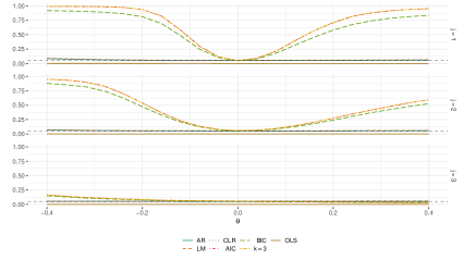
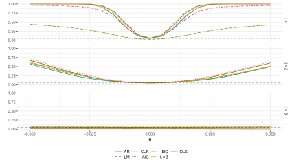
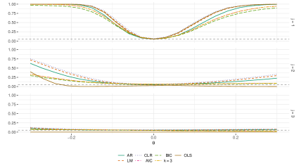
Given the results in Table 9, I consider the power of the $\hat{S}$ tests proposed above and the AR test. These are plotted for the exponential, logistic and linear design in figures 4 – 6. These power plots demonstrate that for the exponential $\pi$ design, there is very limited power available via the AR test. This is not suprising given the linear projections in the definition of the AR statistic. For similar reasons the $\hat{S}$ test with $\pi$ estimated via OLS shows even lower power and never exceeds the nominal 5% level. The $\hat{S}$ tests based on Legendre polynomials by contrast display substantial power in the $j=1,2$ designs. This is as expected, as – unlike the AR test – these tests are able to exploit the non-linear identifying information provided by $Z$.

In the logistic $\pi$ case, no test appears to provide non trivial power for the $j=3$ case (at least over the interval considered). For the $j=1,2$ cases, the AR and $\hat{S}$ tests based on either OLS or Legendre polynomials display similar power.

Finally, in the linear $\pi$ case the (optimal) AR test dominates. In the well identified case ($j=1$) the $\hat{S}$ test based on OLS estimates of $\pi$ matches its power curve, though it performs less well when there is less identifying information. The other $\hat{S}$ tests continue to provide reasonable power in the cases where identification is stronger.

Design 2: Bivariate, just identified

I now consider the case where $d_{\theta}=2$, and $Z_{2}$ is bivariate. $\pi(Z)=\pi(Z_{2})$ will be taken as $\pi(Z_{2})=(\pi_{1}(Z_{2,1}),\pi_{2}(Z_{2,2}))^{\prime}$ with each $\pi_{i}$ ($i=1,2$) being one of the exponential, logistic or linear functions considered in Design 1. The $Z_{2}$ are drawn from a zero - mean, multivariate normal distribution with covariance matrix $\mathrm{Var}(Z_{2})=\left[\begin{smallmatrix}1&0.4\\ 0.4&1\end{smallmatrix}\right]$. The (homoskedastic) error terms $\epsilon,\upsilon$ are drawn (independently) from a zero-mean multivariate normal such that each has variance 1 and the covariances are $\mathrm{Cov}(\epsilon,\upsilon_{i})=0.9$ and $\mathrm{Cov}(\upsilon_{1},\upsilon_{2})=0.7$. As in Design 1, $Z_{1}=1$.

The tests considered are similar to as in Design 1. In particular, I consider the $\hat{S}$ tests with $\pi$ estimated by (i) OLS and (ii) tensor product Legendre polynomials. I consider both fixing the number of polynomials at $k=3$ in each of the univariate series which form the tensor product basis and choosing $k\in\{3,4,5,6,7\}$ using information criteria. $\upnu$ is set to 0.1. I additionally consider the AR test, a TSLS Wald test and GMM Wald and LM tests using the tensor product basis as instruments (along with $Z_{1}$).

The results are shown in Tables 10 & 11. The first table has $\pi_{1}=\pi_{2}$ whilst the second table caries the form of $\pi_{1}$ only, with $\pi_{2}$ always remaining linear. The results are qualitatively similar across the two tables: the $\hat{S}$ test with Legendre polynomials appears to always control the null rejection probability of the test close to the nominal 5% level, as does the AR test. The $\hat{S}$ test with OLS estimates typically underreject. The TSLS Wald test and two GMM tests considered overreject when identification is weaker (higher $j$).

Figures 7 – 15 show power surfaces for the AR test and $\hat{S}$ tests computed with $\pi$ estimated using $k=3$ Legendre polynomials. These are plotted for cases where $\pi_{1}$ and $\pi_{2}$ have the same form and where (i) both $\pi_{1}$ and $\pi_{2}$ have $j=1$, corresponding to a strongly identified setting; (ii) where $\pi_{1}$ has $j=1$ and $\pi_{2}$ has $j=3$, in which $\theta_{2}$ is weakly identified and (iii) where both $\pi_{i}$ have $j=3$, i.e. $\theta$ is weakly identified.

Figures 7 – 9 show the case with exponential $\pi$. For this design the AR test is unable to provide non-trivial power regardless of the identification strength ($j$). In the strongly identified case (i) the $\hat{S}$ test provides good power in all directions. In case (ii), where $\theta_{2}$ is weakly identified, the $\hat{S}$ test continues to provide good power against violations of the null in the first co-ordinate but (as expected) only trivial power in the second co-ordinate. In the weakly identified case (iii), neither test is able to provide reasonable power against the considered alternatives.

For the logistic and linear cases depicted in Figures 10 – 12 and 13 – 15 respectively, all tests display good power in all directions in the strongly identified case (i) and good power against violations of the null in the first co-ordinate but only trivial power against violations in the second co-ordinate in the case (ii) $\theta_{2}$ weakly identified. The AR test seems to provide marginally higher power in these cases, but the difference is minor with both tests displaying similar power surfaces. In case (iii) where $\theta$ is weakly identified, the $\hat{S}$ test displays only trivial power. The same is true of the AR test in the logistic design; it is able to provide some power in one corner of the plot for the linear design.

Some additional simulation results for this design are reported in section S4.2.1 in the supplementary material. In particular, these results highlight that choosing the number of polynomial basis functions $k$ by AIC yields power surfaces which are typically very similar to those in Figures 7 – 15.

Additional simulation results

Section S4 contains a discussion of two further simulation designs, which I briefly summarise here. Design 3 replicates Design 1 with the addition of heteroskedastic errors. Briefly, the results are qualitiatively the same as found in Design 1 with the $\hat{S}$ tests well controlling the empirical rejection frequency in each scenario. As in the homoskedastic case, the $\hat{S}$ test provides substantially higher power than the AR test when $\pi$ is exponential, and competitive power with the AR test in the logistic and the linear cases.

Design 4 considers an over-identified model. Specifically, the base setup is as in Design 1 (with $\rho=0.95$ and Gaussian errors), however $Z_{2}$ is bivarate mean-zero normal with $\mathrm{Var}(Z_{2})=\left[\begin{smallmatrix}1&0.4\\ 0.4&1\end{smallmatrix}\right]$ and $\pi(Z_{2})=(\pi_{1}(Z_{2,1})+\pi_{2}(Z_{2,2}))/2$ where $\pi_{1}$ and $\pi_{2}$ have one of the exponential, logistic or linear forms of Table 8. For the $\hat{S}$ tests, $\pi$ is estimated in the same manner as for Design 2: using series regressions on tensor product bases formed of Legendre polynomials. A version with $\pi$ estimated using OLS on $Z_{2}$ (and a constant) is also reported, along with GMM Wald and LM tests using these tensor product bases as instruments, the TSLS Wald test and AR, LM (Kleibergen, 2002) and CLR (Moreira, 2003) tests.

The results show that both the “usual” weak instrument robust tests (AR, LM and CLR) and the $\hat{S}$ tests are able to well control the null rejection frequency, unlike the TSLS Wald and GMM based tests. In terms of power, the results are similar to the other designs: in the exponential case the $\hat{S}$ tests with nonparametrically estimated $\pi$ are the only tests able to provide non-trivial power regardless of identification strength. In the logistic and linear cases, the $\hat{S}$ tests typically provide comparable power to the LM and CLR tests, with the latter two tests performing slightly better in the linear cases.

5 Empirical applications

In this section I apply the test developed in section 4.2 for the IV model (Example 2) to two classic instrumental variables studies.

5.1 Institutions and economic performance

Acemoglu et al. (2001) investigate the effect of better intitutions (i.e. better property rights, less distortionary policies) on economic performance. They use a measure of the average protection against expropriation risk as a measure of the strength of insitutions. Due to potential endogeneity concerns, they instrument this variable by the mortality rates of European colonial settlers. In the notation of Example 2, $Y$ is the 1995 log gdp per capita on a ppp basis, $X$ is a measure of the risk of government expropriation of private foreign investment, $Z_{1}$ contains a constant and any exogenous variables in the given specifications and $Z_{2}$ is the log of a measure of European settler mortality. I refer to the original article Acemoglu et al. (2001) for more detail on the data and a discussion of the literature.

Table 4 in Acemoglu et al. (2001) provides their two-stage least squares estimates for a variety of specifications along with the associated (Wald) confidence intervals; for details of the specifications, see Acemoglu et al. (2001). Table 1 below replicates these results (for specifications (1) – (8)), along with: (i) the first stage $F$ statistic; (ii) OLS point estimates and the associated (Wald) confidence intervals; (iii) weak instrument robust Anderson and Rubin (1949) (hereafter AR) confidence intervals and (iv) weak instrument robust confidence intervals formed by inverting the $\hat{S}$ test developed in Section 4.2. This is implemented using

$$\hat{\pi}(Z)=\hat{\alpha}_{1}^{\prime}\tilde{Z}_{1}+\hat{\alpha}_{2}^{\prime}p_{k}(Z_{2}),$$

with $p_{k}$ the first $k$ Legendre orthogonal polynomials, $\tilde{Z}_{1}$ is $Z_{1}$ excluding the constant term. and $\hat{\alpha}$ is the OLS estimate in the regression of $X$ on $(\tilde{Z}_{1},p_{k}(Z_{2}))$. $k$ is chosen via AIC, the truncation parameter $\upnu=0.001$ and the test is inverted over an evenly spaced grid of 1000 points between -1 and 3.

As can be see in Table 1, the first stage $F$ statistic for many of the considered specifications is below the rule-of-thumb cutoff of 10 proposed by Staiger and Stock (1997) and so there is suggestive evidence that the instruments may be weak in these specifications.

Overall the $\hat{S}$ based confidence intervals do not change the conclusions of Acemoglu et al. (2001) – all the confidence intervals exclude zero and and suggest similarly sized effects as found by Acemoglu et al. (2001). The results do however demonstrate that the ability of the $\hat{S}$ test to exploit potential non-linearities in the relationship between the endogenous variable and instrument can result in (test inversion) confidence intervals which are much shorter than the AR confidence intervals (whilst remaining robust to weak identification). Table 2 shows the lengths of the OLS, 2SLS and $\hat{S}$ confidence intervals as a fraction of the length of the AR confidence interval for specifications (1) – (7) (specification (8) is excluded due to the AR confidence interval having infinite length). In all specifications inverting the $\hat{S}$ test produces a shorter confidence interval than inverting the AR test: the reduction in length ranges from around a $75\%$ reduction in specification (7) to essentially no reduction in specification (5).

Table 1: Point estimates and confidence intervals

	(1)	(2)	(3)	(4)	(5)	(6)	(7)	(8)
$n$	64	64	60	60	37	37	64	64
$F$	22.95	13.09	8.65	7.83	30.54	21.61	6.23	3.46
$k$	3	3	4	4	1	1	3	3
Point estimates
OLS	0.52	0.47	0.49	0.47	0.48	0.47	0.42	0.4
2SLS	0.94	1	1.28	1.21	0.58	0.58	0.98	1.11
Confidence intervals
OLS	$[0.4,0.64]$	$[0.34,0.6]$	$[0.33,0.64]$	$[0.32,0.62]$	$[0.35,0.61]$	$[0.32,0.61]$	$[0.31,0.54]$	$[0.28,0.52]$
2SLS	$[0.63,1.26]$	$[0.55,1.44]$	$[0.56,2]$	$[0.5,1.92]$	$[0.38,0.78]$	$[0.34,0.81]$	$[0.38,1.58]$	$[0.18,2.04]$
AR	$[0.7,1.43]$	$[0.68,1.88]$	$[0.81,3.33]$	$[0.75,3.44]$	$[0.39,0.82]$	$[0.35,0.89]$	$[0.6,3.59]$	$(-\infty,-9.24]\cup[0.59,\infty)$
$S$	$[0.58,1.05]$	$[0.47,0.97]$	$[0.26,1.12]$	$[0.02,0.97]$	$[0.41,0.84]$	$[0.36,0.85]$	$[0.32,1.09]$	$[0.26,0.97]$

• Notes: $F$ is the first stage $F$ statistic; $k$ is the number of polynomials in $Z_{2}$ chosen by AIC.

Table 2: Length of confidence interval relative to AR

	(1)	(2)	(3)	(4)	(5)	(6)	(7)
OLS	0.335	0.213	0.121	0.110	0.611	0.535	0.077
2SLS	0.857	0.736	0.571	0.526	0.922	0.888	0.401
AR	1.000	1.000	1.000	1.000	1.000	1.000	1.000
$S$	0.647	0.416	0.344	0.354	0.992	0.917	0.256

5.2 Returns to schooling

I revisit the problem of estimating the returns to schooling using IV methods. In particular I use the data from the original Card (1995) article: 1976 wage data and education data from the 1966 NLS cohort. See Card (1995) for details on the dataset and Card (2001) for a review of the literature. I set $Y$ to be the log wage in 1976, $X$ the years of education, $Z_{2}$ is an indicator for growing up near a 4 – year college interacted with father’s education, and $Z_{1}$ includes an intercept and controls for race, experience, SMSA and region.

Table 3 below provides (i) OLS and (ii) two-stage least squares estimates along with their associated (Wald) confidence intervals, (iii) weak instrument robust AR confidence intervals and (iv) weak instrument robust confidence intervals formed by inverting the $\hat{S}$ test developed in Section 4.2. This is implemented using

$$\hat{\pi}(Z)=\hat{\alpha}_{1}^{\prime}\tilde{Z}_{1}+\hat{\alpha}_{2}^{\prime}p_{k}(Z_{2}),$$

with $p_{k}$ the first $k$ Legendre orthogonal polynomials, $\tilde{Z}_{1}$ is $Z_{1}$ excluding the constant term. and $\hat{\alpha}$ is the OLS estimate in the regression of $X$ on $(\tilde{Z}_{1},p_{k}(Z_{2}))$. AIC chooses $k=2$, the truncation parameter is set to $\upnu=0.001$ and the test is inverted over an evenly spaced grid of 1000 points between -0.2 and 0.2.

Table 3: Point estimates and confidence intervals

Method	Point Estimate	Confidence Interval	Relative Length
OLS	0.076	$[0.069,0.084]$	0.178
2SLS	0.085	$[0.043,0.128]$	0.975
AR		$[0.042,0.13]$	1.000
$S$		$[0.042,0.118]$	0.868

The confidence interval obtained by inverting the $\hat{S}$ test is similar but slightly shorter than the AR interval, achieving an approximate $15\%$ reduction in length.

6 Conclusion

In this paper I introduced a notion of local regularity for (sequences of) tests analogous to the notion of local regularity for estimators widely used in semiparametric estimation theory. I established that C($\alpha$) – style tests are locally regular under mild conditions, including in non – regular cases where locally regular estimators do not exist. Such non – regular cases include, for example, semiparametric weak identification asymptotics.

I additionally generalised the classical local asymptotic power bounds for locally asymptotically normal semiparametric models to the case where the efficient information matrix has positive, but potentially deficient, rank. As such, these results also apply in cases of underidentification (or weak underidentification). Moreover, I demonstrated that, for a certain choice of moment function, the C($\alpha$) – style test attains these power bounds. This improves on known results as it does not require the data to be i.i.d. nor the information operator to be boundedly invertible.

Three examples are developed in detail and the approach is validated in simulation studies which demonstrate that the asymptotic theory provides an accurate approximation to the finite sample performance of the considered C($\alpha$) tests. In particular, it is shown that in a single-index model, the considered C$(\alpha)$ test is robust to plugging in a shape constrained estimator of the link function, whilst in a IV model, the considered C$(\alpha)$ test remains robust under semiparametric weak identification asymptotics and can have substantially higher power than classical weak instrument robust tests when the relationship between the endogenous variables and instruments is non-linear. This latter point is also highlighted in two empirical examples using the IV model in which inverting the C($\alpha$) test can lead to substantially shorter confidence intervals than the Anderson and Rubin (1949) test.

Appendix A Proofs of the main results

Proof of Proposition 1.

Combination of Assumptions 1 and 2 yields

$$\left(g^{\prime}_{n,\theta,\lambda},L_{n,\gamma}(h)\right)\overset{P_{n,\gamma,0}}{\rightsquigarrow}\mathcal{N}\left(\begin{pmatrix}0\\ -\frac{1}{2}\sigma_{\gamma}(h)\end{pmatrix},\begin{pmatrix}V_{\gamma}&\tau^{\prime}\Sigma_{\gamma,21}^{\prime}\\ \Sigma_{\gamma,21}\tau&\sigma_{\gamma}(h)\end{pmatrix}\right).$$

Consequently, by Le Cam’s third Lemma (e.g. van der Vaart, 1998, Example 6.7)

$$g_{n,\gamma}\overset{P_{n,\gamma,h}}{\rightsquigarrow}Z_{\tau}\mathcal{N}\left(\Sigma_{\gamma,21}\tau,V_{\gamma}\right).$$

The second claim follows by combining the preceding display with Assumption 3(i), Remark 1 and Slutsky’s Theorem. Combining the second claim with Assumption 3(ii), Slutsky’s Theorem and the continuous mapping Theorem, the asymptotic distribution of $\hat{S}_{n,\theta}$ under $P_{n,\gamma,h}$ is the law of

$$Z^{\prime}V_{\gamma}^{\dagger}Z,\qquad Z\sim\mathcal{N}\left(\Sigma_{\gamma,21}\tau,V_{\gamma}\right),$$

which is the indicated non-central $\chi^{2}_{r}$ (Rao and Mitra, 1971, Theorem 9.2.3). ∎

Proof of Theorem 1.

As $\hat{r}_{n}\xrightarrow{P_{n,\gamma}}r$, $P_{n,\gamma}\{c_{n}=c_{\alpha}\}\to 1$. By Proposition 1, Remark 1 and Slutsky’s Theorem, $\hat{S}_{n,\theta}-c_{n}\rightsquigarrow S-c$ under $P_{n,\gamma,h}$ where $S\sim\chi^{2}_{r}\left(a\right)$. Since the $\chi^{2}_{r}$ distribution is continuous, by the Portmanteau Theorem,

$$\lim_{n\to\infty}P_{n,\gamma,h}\psi_{n,\theta}=\lim_{n\to\infty}P_{n,\gamma,h}\left(\hat{S}_{n,\theta}>c_{n}\right)=L\{S-c>0\}=1-\mathrm{P}(\chi_{r}^{2}(a)\leq c_{\alpha}),$$

for $L$ the law of $S$. For the second result, note that if $\operatorname{rank}(\hat{\Lambda}_{n,\theta})\xrightarrow{P_{n,\gamma}}r=0$, then $P_{n,\gamma}(R_{n})\to 1$ for $R_{n}\coloneqq\{\hat{\Lambda}_{n,\theta}=0\}$. On this set $\hat{S}_{n,\theta}=0$ and so $\psi_{n,\theta}=0$. By Remark 1, $P_{n,\gamma,h}(R_{n})\to 1$ and therefore $P_{n,\gamma,h}\psi_{n,\theta}\leq 1-P_{n,\gamma,h}(R_{n})\to 0$. ∎

Proof of Corollary 1.

Since $\tau=0$, $\chi^{2}_{r}(a)=\chi^{2}_{r}(0)=\chi^{2}_{r}$, and hence $\mathrm{P}(\chi^{2}_{r}(a)\leq c_{\alpha})=1-\alpha$. Apply Theorem 1 along the stated sequences. ∎

Proof of Corollary 2.

$P_{n,\gamma,h_{n}}(\theta\in C_{n})=1-P_{n,\gamma,h_{n}}\psi_{n,\theta}$. Apply Corollary 1. ∎

Proof of Corollary 3.

Let $\uppi_{n}(h)\coloneqq P_{n,\gamma,h}\psi_{n,\theta}$ and $\uppi(h)\coloneqq 1-\mathrm{P}(\chi^{2}_{r}(a)\leq c_{r})$ if $r\geq 1$ or $\uppi(h)\coloneqq 0$ if $r=0$. By Remark 4, $\uppi_{n}(h)\to\uppi(h)$ pointwise in $h\in H_{\gamma}$. Since the $\uppi_{n}$ are asymptotically equicontinuous on $K$, the convergence is also uniform on $K$. ∎

Proof of Corollary 4.

Let $\uppi_{n}(h)\coloneqq P_{n,\gamma,h}\psi_{n,\theta}$ and $\uppi(h)\coloneqq\alpha\bm{1}\{r\geq 1\}$. By Corollary 1, $\uppi_{n}(h)\to\uppi(h)\eqqcolon c$ pointwise in $h\in H_{\gamma,0}$. Since the $\uppi_{n}$ are asymptotically equicontinuous on $K$, the convergence is also uniform on $K$. Hence,

$$\lim_{n\to\infty}\sup_{h\in K}\uppi_{n}(h)\leq\lim_{n\to\infty}\sup_{h\in K}\left|\uppi_{n}(h)-c\right|+c=c=\uppi(h).\qed$$

Proof of Lemma 1.

This follows from (e.g. Strasser, 1985, Theorem 2.3)

$$\left|P_{n,\gamma,h}\psi_{n,\theta}-P_{n,\gamma,h^{\prime}}\psi_{n,\theta}\right|\leq d_{TV}(P_{n,\gamma,h},P_{n,\gamma,h^{\prime}}).\qed$$

Proof of Lemma 2.

The proof is given for the case where $(H_{\gamma},d)$ is a pseudometric space and $K\subset H_{\gamma}$. The argument in the case with $H_{\gamma,0}$ replacing $H_{\gamma}$ is analogous. First suppose $r\geq 1$. By asymptotic equicontinuity of $h\mapsto Q_{n,\gamma,h}$ on $K$, for any $h_{n}\to h$ (through $K$), $\lim_{n\to\infty}\delta(Q_{n,\gamma,h_{n}},Q_{n,\gamma,h})=0$ and by the asymptotic equicontinuity (on $K$) of $h\mapsto P_{n,\gamma,h}(\hat{r}_{n,\theta}=r)$, $\lim_{n\to\infty}|P_{n,\gamma,h}(\hat{r}_{n,\theta}=r)-P_{n,\gamma,h_{n}}(\hat{r}_{n,\theta}=r)|=0$. Since $\hat{r}_{n,\theta}\xrightarrow{P_{n,\gamma,h}}r$ (Assumption 3 (iii) and Remark 1), it follows that also $\hat{r}_{n,\theta}\xrightarrow{P_{n,\gamma,h_{n}}}r$. Hence, under $P_{n,\gamma,h_{n}}$,

$$\hat{S}_{n,\theta}-c_{n}\rightsquigarrow S-c_{r},\quad S\sim\chi^{2}_{r}(a)\implies P_{n,\gamma,h_{n}}\varphi_{n,\theta}\to 1-\mathrm{P}(\chi^{2}_{r}(a)\leq c_{r})\eqqcolon\uppi(\tau),$$

by Proposition 1 where $c_{r}$ and $a$ are as in Theorem 1. Thus, by Theorem 1,

$$|P_{n,\gamma,h_{n}}\varphi_{n,\theta}-P_{n,\gamma,h}\varphi_{n,\theta}|\leq|P_{n,\gamma,h_{n}}\varphi_{n,\theta}-\uppi(\tau)|+|P_{n,\gamma,h}\varphi_{n,\theta}-\uppi(\tau)|\to 0,$$

which implies the required asymptotic equicontinuity on $K$.

In the case where $r=0$, the asymptotic equicontinuity on $K$ of $h\mapsto P_{n,\gamma,h}(\hat{\Lambda}_{n,\theta}=0)$ implies that if $h_{n}\to h$ (through $K$), $|P_{n,\gamma,h_{n}}(\hat{\Lambda}_{n,\theta}=0)-P_{n,\gamma,h}(\hat{\Lambda}_{n,\theta}=0)|\to 0$ as $n\to\infty$. In combination with $\operatorname{rank}(\hat{\Lambda}_{n,\theta})\xrightarrow{P_{n,\gamma,h}}0$ (Assumption 3 (iii) and Remark 1), this implies that $P_{n,\gamma,h_{n}}(\hat{\Lambda}_{n,\theta}=0)\to 1$ and thus $P_{n,\gamma,h_{n}}\varphi_{n,\theta}\to 0$. Thus, by Theorem 1

$$|P_{n,\gamma,h_{n}}\varphi_{n,\theta}-P_{n,\gamma,h}\varphi_{n,\theta}|\leq|P_{n,\gamma,h_{n}}\varphi_{n,\theta}|+|P_{n,\gamma,h}\varphi_{n,\theta}|\to 0,$$

which implies the required asymptotic equicontinuity on $K$. ∎

Proof of Lemma 3.

For $a,b\in\mathbb{R}$ and $h_{1},h_{2}\in H_{\gamma}$ we have

$$\Delta_{n,\gamma}(a_{1}h_{1}+a_{2}h_{2})=a_{1}\Delta_{n,\gamma}h_{1}+a_{2}\Delta_{n,\gamma}h_{2}$$

and in consequence $\Delta_{\gamma}(a_{1}h_{1}+a_{2}h_{2})=a_{1}\Delta_{\gamma}(h_{1})+a_{2}\Delta_{\gamma}(h_{2})$, hence $\Delta_{\gamma}$ is linear. We next note that $K_{\gamma}$ is well-defined and a bilinear, symmetric, positive semidefinite (i.e. covariance) kernel. Firstly, since for $h\in H_{\gamma}$, we have $\sigma_{\gamma}(h)=\lim_{n\to\infty}\|\Delta_{n,\gamma}h\|^{2}$, $(\|\Delta_{n,\gamma}h\|^{2})_{n\in\mathbb{N}}$ is bounded and Cauchy (in $\mathbb{R}$). Letting $K_{n,\gamma}(h,g)\coloneqq P_{n,\gamma}\left[\Delta_{n,\gamma}h\Delta_{n,\gamma}g\right]$ and using Cauchy – Schwarz

$$\left|K_{n,\gamma}(h,g)-K_{m,\gamma}(h,g)\right| \leq|P_{n,\gamma}\left[(\Delta_{n,\gamma}h-\Delta_{m,\gamma}h)\Delta_{n,\gamma}g\right]+P_{n,\gamma}\left[\Delta_{m,\gamma}h(\Delta_{n,\gamma}g-\Delta_{m,\gamma}g)\right]$$

$$\leq\|\Delta_{n,\gamma}h-\Delta_{m,\gamma}h\|\|\Delta_{n,\gamma}g\|+\|\Delta_{m,\gamma}h\|\|\Delta_{n,\gamma}g-\Delta_{m,\gamma}g\|,$$

hence $(K_{n,\gamma}(h,g))_{n\in\mathbb{N}}$ is also Cauchy and thus has a limit in $\mathbb{R}$. Bilinearity of $K_{\gamma}$ follows directly from its definition and the linearity of $\Delta_{n,\gamma}$. Symmetry follows from the symmetry of multiplication in $\mathbb{R}$. For positive semi-definiteness, let $h_{1},\ldots,h_{K}\in H_{\gamma}$, $a\in\mathbb{R}^{K}$. Since each $\Delta_{n,\gamma}h\in L_{2}^{0}(P_{n,\gamma})$, each matrix $\mathcal{K}_{n}\coloneqq[K_{n,\gamma}(h_{k},h_{j})]_{k,j=1}^{K}$ is a covariance matrix and hence positive semi-definite. Therefore, for each $n$,

$$\sum_{k=1}^{K}\sum_{j=1}^{K}a_{k}a_{j}K_{n,\gamma}(h_{k},h_{j})=a^{\prime}\mathcal{K}_{n}a\geq 0,$$

hence the same holds in the limit, i.e. with $K_{n,\gamma}$ and $\mathcal{K}_{n}$ replaced by $K_{\gamma}$ and $\mathcal{K}\coloneqq[K_{\gamma}(h_{k},h_{j})]_{k,j=1}^{K}$ respectively.

Finally, by Assumption 1 and the fact that $K(h,h)=\sigma_{\gamma}(h)$, $\Delta_{\gamma}h\sim\mathcal{N}(0,K(h,h))$. Using this along with the linearity of $\Delta_{n,\gamma}$, $\Delta_{\gamma}$ and the bilinearity of $K$,

$$\sum_{k=1}^{K}a_{k}\Delta_{n,\gamma}(h_{k})=\Delta_{n,\gamma}\left(\sum_{k=1}^{K}a_{k}h_{k}\right)\overset{P_{n,\gamma}}{\rightsquigarrow}\Delta_{\gamma}\left(\sum_{k=1}^{K}a_{k}h_{k}\right)=\sum_{k=1}^{K}a_{k}\Delta_{\gamma}h_{k}\sim\mathcal{N}\left(0,a^{\prime}\mathcal{K}a\right),$$

where $\mathcal{K}\coloneqq[K(h_{k},h_{j})]_{k,j=1}^{K}$. Therefore, by the Cramér – Wold Theorem, $\Delta_{\gamma}$ is a mean-zero Gaussian process with covariance kernel $K$. ∎

Proof of Proposition 2.

Remark 1 and the transitivity of (mutual) contiguity ensures that the experiments $\mathscr{E}_{n,\gamma}$ are contiguous (cf. Strasser, 1985, Definition 61.1). Hence by Theorem 61.6 of Strasser (1985) it suffices to show that the finite dimensional marginal distributions of $h\mapsto L_{n,\gamma}(h)$ converge (under $P_{n,\gamma}$) to those of $h\mapsto L(h)\coloneqq\Delta_{\gamma}h-\frac{1}{2}\|h\|_{\gamma}^{2}$. For this it is enough to note that the finite dimensional marginal distributions of $\Delta_{n,\gamma}$ converge to those of $\Delta_{\gamma}$ (under $P_{n,\gamma}$), as follows by the Cramér – Wold Theorem (as in the proof of Lemma 3). ∎

Proof of Proposition 3.

Let $G_{[0]}\coloneqq P_{\gamma,0}$. Define a map $Z:\mathbb{H}_{\gamma}\to L_{2}(\Omega,\mathcal{F},G_{[0]})$ according to $Z[h]=\Delta_{\gamma}(h)$ for any arbitrary $h\in\pi_{V}^{-1}([h])$, where $\pi_{V}$ is the quotient map from $H_{\gamma}\to\mathbb{H}_{\gamma}$; that this is well defined is noted in footnote 59. By the definition of $\left\langle{\cdot}\,,\,{\cdot}\right\rangle_{\gamma}$ on $\mathbb{H}_{\gamma}$ (cf. subsection S2.2) this is a standard Gaussian process for $\mathbb{H}_{\gamma}$. Let each $G_{[h]}$ be defined such that

$$\frac{\mathrm{d}G_{[h]}}{\mathrm{d}G_{[0]}}=\exp\left(Z[h]-\frac{1}{2}\|[h]\|_{\gamma}^{2}\right),$$

and note that by Theorem 69.4 in Strasser (1985), $\mathscr{G}_{\gamma}$ is a Gaussian shift on $(\mathbb{H}_{\gamma},\left\langle{\cdot}\,,\,{\cdot}\right\rangle_{\gamma})$.

For any $h\in H_{\gamma}$ we have that $Z[h]=\Delta_{\gamma}g$ for some $g\in\pi_{V}^{-1}([h])$ and $\Delta_{\gamma}h=\Delta_{\gamma}g$ $P_{\gamma,0}$–almost surely by footnote 59. Since $\|h\|_{\gamma}=\|[h]\|_{\gamma}$ (cf. subsection S2.2) one therefore has that

$$\frac{\mathrm{d}G_{[h]}}{\mathrm{d}G_{[0]}}=\exp\left(Z[h]-\frac{1}{2}\|[h]\|_{\gamma}^{2}\right)=\exp\left(\Delta_{\gamma}h-\frac{1}{2}\|h\|_{\gamma}^{2}\right)=\frac{\mathrm{d}P_{\gamma,h}}{\mathrm{d}P_{\gamma_{0}}},\quad P_{\gamma,0}\text{ -- a.s.}.$$

By construction, each $P_{\gamma,h}$ and $G_{[h]}$ is absolutely continuous with respect to $P_{\gamma,0}=G_{[0]}$. Hence, by Lemma 2.4 in Strasser (1985),

$$d_{TV}(P_{\gamma,h},G_{[h]})=\frac{1}{2}\int\left|\frac{\mathrm{d}P_{\gamma,h}}{\mathrm{d}P_{\gamma_{0}}}-\frac{\mathrm{d}G_{[h]}}{\mathrm{d}P_{\gamma_{0}}}\right|\,\mathrm{d}P_{\gamma,0}=\frac{1}{2}\int\left|\frac{\mathrm{d}P_{\gamma,h}}{\mathrm{d}P_{\gamma_{0}}}-\frac{\mathrm{d}G_{[h]}}{\mathrm{d}G_{[0]}}\right|\,\mathrm{d}P_{\gamma,0}=0.\qed$$

Proof of Lemma 4.

We have that

$$\left\langle{[(\tau,b)]}\,,\,{([t,g)]}\right\rangle_{\gamma} =\left\langle{[(\tau,0)]+[(0,b)]}\,,\,{[(t,0)]+[(0,g)]}\right\rangle_{\gamma}$$ (44)

$$=\left\langle{\Pi^{\perp}[(\tau,0)]+\Pi[(\tau,0)]+[(0,b)]}\,,\,{\Pi^{\perp}[(t,0)]+\Pi[(t,0)]+[(0,g)]}\right\rangle_{\gamma}$$

$$=\left\langle{\Pi^{\perp}[(\tau,0)]}\,,\,{\Pi^{\perp}[(t,0)]}\right\rangle_{\gamma}+\left\langle{\Pi[(\tau,0)]+[(0,b)]}\,,\,{\Pi[(t,0)]+[(0,g)]}\right\rangle_{\gamma}$$

$$=\tau^{\prime}\tilde{\mathcal{I}}_{\gamma}t+\left\langle{\Pi[(\tau,0)]+[(0,b)]}\,,\,{\Pi[(t,0)]+[(0,g)]}\right\rangle_{\gamma}.$$

From this and the fact that $\Pi[(\tau,0)]\in\ker\pi_{1}$, we obtain

$$\|[\tau]\|^{2}=\inf_{b\in B_{\gamma}}\|[(\tau,b)]\|^{2}_{\gamma}=\inf_{[h]\in\ker\pi_{1}}\|[(\tau,0)]-[h]\|^{2}_{\gamma}=\tau^{\prime}\tilde{\mathcal{I}}_{\gamma}\tau+\inf_{[h]\in\ker\pi_{1}}\|\Pi[(\tau,0)]-[h]\|^{2}_{\gamma}=\tau^{\prime}\tilde{\mathcal{I}}_{\gamma}\tau.$$

Hence, if $\|\tau\|=\|[\tau]\|=0$, it follows that $\tau^{\prime}\tilde{\mathcal{I}}_{\gamma}\tau=0$. Hence $\tilde{\mathcal{I}}_{\gamma}^{1/2}\tau=0$. But then $\tilde{\mathcal{I}}_{\gamma}\tau=\tilde{\mathcal{I}}_{\gamma}^{1/2}\tilde{\mathcal{I}}_{\gamma}^{1/2}\tau=0$. Conversely suppose that $\tau\in\ker\tilde{\mathcal{I}}_{\gamma}$. Then, $\|\tau\|^{2}=\tau^{\prime}\tilde{\mathcal{I}}_{\gamma}\tau=0$ and hence $\|\tau\|=0$. ∎

Proof of Lemma 5.

Let $V\coloneqq\{h\in H_{\gamma}:\|h\|_{\gamma}=0\}$ and let $\pi_{V}:H_{\gamma}\to\mathbb{H}_{\gamma}=H_{\gamma}\,/\,V$ be the canonical projection. For $h\in H_{\gamma}$ we write $[h]\coloneqq\pi_{V}(h)$. Define $Z:\overline{\mathbb{H}_{\gamma}}\to L_{2}(\mathrm{P})$ as $Z[h]=\Delta_{\gamma}(h)$, which is a mean-zero linear Gaussian process with covariance kernel $K([h],[g])=K_{\gamma}(h,g)=\left\langle{[h]}\,,\,{[g]}\right\rangle_{\gamma}$. $Y\coloneqq\operatorname{ran}Z\subset L_{2}(\mathrm{P})$ is evidently a linear space and

$$\left\langle{[h]}\,,\,{[g]}\right\rangle\coloneqq\mathbb{E}\left[Z[h]Z[g]\right]=K([h],[g])=\left\langle{[h]}\,,\,{[g]}\right\rangle_{\gamma},\quad[h],[g]\in\overline{\mathbb{H}_{\gamma}}.$$

The above display and the completeness of $\overline{\mathbb{H}_{\gamma}}$ yield the closedness of $\operatorname{ran}Z$. Hence $Z$ is a Hilbert space isomorphism from $\overline{\mathbb{H}_{\gamma}}$ to $Y$. As such it is bijective, with $Z^{*}=Z^{-1}$. We have

$$\mathcal{T}=\{\Delta_{\gamma}(h):h=(0,b)\in H_{\gamma}\}=\{Z[h]:h=(0,b)\in H_{\gamma}\}=\{Z[h]:[h]\in\ker\pi_{1}^{\prime}\},$$

where $\pi_{1}^{\prime}$ denotes the restriction of $\pi_{1}$ to $\mathbb{H}_{\gamma}$. We next note that $\mathcal{T}^{\perp}=\{Z[h]:[h]\in(\ker\pi_{1})^{\perp}\}$. For the first inclusion suppose that $Z[g]\in\mathcal{T}^{\perp}$. Then, for any $[h]\in\ker\pi_{1}^{\prime}$,

$$\left\langle{[g]}\,,\,{[h]}\right\rangle_{\gamma}=\left\langle{Z[g]}\,,\,{Z[h]}\right\rangle_{L_{2}(P)}=0.$$

Since $\ker\pi_{1}=\operatorname{cl}\ker\pi_{1}^{\prime}$ by Lemma S1, for any $[h]\in\ker\pi_{1}$ there is a sequence in $\ker\pi_{1}^{\prime}$ which converges to $[h]$ and the result follows by taking limits. For the other inclusion note that a corollary of Lemma S1 is that $(\ker\pi_{1})^{\perp}=(\ker\pi_{1}^{\prime})^{\perp}$. Hence, if $[g]\in(\ker\pi_{1})^{\perp}$, for any $[h]\in\ker\pi_{1}^{\prime}$ we have

$$\left\langle{Z[g]}\,,\,{Z[h]}\right\rangle_{L_{2}(P)}=\left\langle{[g]}\,,\,{[h]}\right\rangle=0.$$

Let $Q$ denote the orthogonal projection on $(\ker\pi_{1})^{\perp}\subset\overline{\mathbb{H}_{\gamma}}$ and $R$ that on $\mathcal{T}^{\perp}\subset Y$. Since $Z$ is a Hilbert space isomorphism one has

$$R\Delta_{\gamma}(h)=RZ[h]=ZQZ^{*}Z[h]=ZQZ^{-1}Z[h]=ZQ[h],\quad[h]\in\overline{\mathbb{H}_{\gamma}}.$$

Hence for $[h]=[e_{i},0]$, $RZ[e_{i},0]=ZQ[e_{i},0]$ implying

$$\mathbb{E}\left[\tilde{\Delta}_{\gamma}(e_{i},0)\tilde{\Delta}_{\gamma}(e_{j},0)\right]=\left\langle{\Pi^{\perp}[e_{i},0]}\,,\,{\Pi^{\perp}[e_{j},0]}\right\rangle_{\gamma}=\tilde{\mathcal{I}}_{\gamma,ij}.\qed$$

Proof of Theorem 2.

Define the bounded linear map $T:\overline{\mathbb{H}_{\gamma}}\to\mathbb{R}$ as

$$T[h]\coloneqq\left\langle{\Pi^{\perp}[1,0]}\,,\,{\Pi^{\perp}[h]}\right\rangle_{\gamma}=\left\langle{\Pi^{\perp}[1,0]}\,,\,{[h]}\right\rangle_{\gamma}.$$

The equality in the preceding display follows from the idempotentcy and self-adjointness of orthogonal projections. The boundedness of $T$ follows from the Cauchy - Schwarz inequality as orthogonal projections have norm one. For any $[h]=[\tau,b]\in\mathbb{H}_{\gamma}$,

$$T[h]=\left\langle{\Pi^{\perp}[1,0]}\,,\,{\Pi^{\perp}[\tau,b]}\right\rangle_{\gamma}=\tilde{\mathcal{I}}_{\gamma}\tau.$$ (45)

Assume first that $\sqrt{\tilde{\mathcal{I}}_{\gamma}}\neq 0$, hence $\operatorname{rank}(\tilde{\mathcal{I}}_{\gamma})=1$. Then, let $[u]=\frac{\Pi^{\perp}[1,0]}{\sqrt{\tilde{\mathcal{I}}_{\gamma}}}$ and note that $\|[u]\|=1$ and for any $[h]\in\ker T$, $\left\langle{[u]}\,,\,{[h]}\right\rangle_{\gamma}=\frac{1}{\sqrt{\tilde{\mathcal{I}}_{\gamma}}}T[h]=0$, hence $[u]\in[\ker T]^{\perp}$ and $T[u]=\sqrt{\tilde{\mathcal{I}}_{\gamma}}>0$. Lemma 71.5 in Strasser (1985) ensures that any unbiased level $\alpha$ test $\phi$ of $K_{0}:T[h]=0$ against $K_{1}:T[h]\neq 0$ in the (restricted) Gaussian shift $\mathscr{G}_{\gamma}$ satisfies

$$G_{[h]}\phi\leq 1-\Phi\left(z_{\alpha/2}-\tilde{\mathcal{I}}_{\gamma}^{1/2}\tau\right)+1-\Phi\left(z_{\alpha/2}+\tilde{\mathcal{I}}_{\gamma}^{1/2}\tau\right)$$ (46)

By Proposition 2, $\mathscr{E}_{n,\gamma}\rightsquigarrow\mathscr{E}_{\gamma}$ where the latter is dominated. Let $\uppi_{n}(h)\coloneqq P_{n,\gamma,h}\phi_{n}$ and fix an arbitrary $h^{\star}$ for which the bound will be shown. There is a subsequence $(n_{m})_{m\in\mathbb{N}}$ along which $\lim_{m\to\infty}\uppi_{n_{m}}(h^{\star})=\limsup_{n\to\infty}\uppi_{n}(h^{\star})$. Since $[0,1]^{H_{\gamma}}$ is compact in the product topology, there is a subnet $(n_{m(s)})_{s\in S}$ of $(n_{m})_{m\in\mathbb{N}}$ and a function $\uppi:H_{\gamma}\to[0,1]$ such that $\lim_{s\in S}\uppi_{n_{m(s)}}(h)=\uppi(h)$ for all $h\in H_{\gamma}$. By our hypotheses and equation (45) for any $h_{0}$ such that $[h_{0}]\in\ker T\cap\mathbb{H}_{\gamma}$ and any $h_{1}$ such that $[h_{1}]\in\mathbb{H}_{\gamma}\setminus(\ker T\cap\mathbb{H}_{\gamma})$

$$\uppi(h_{0})=\lim_{s\in S}\uppi_{n_{m(s)}}(h_{0})\leq\alpha\leq\lim_{s\in S}\uppi_{n_{m(s)}}(h_{1})=\uppi(h_{1}).$$

Theorem 7.1 in van der Vaart (1991) ensures the existence of a test $\phi$ in $\mathscr{E}_{\gamma}$ with power function $\uppi$. The above display and Proposition 3 ensures that $\phi$ is an unbiased and level $\alpha$ test of $\ker T\cap\mathbb{H}_{\gamma}$ against $\mathbb{H}_{\gamma}\setminus(\ker T\cap\mathbb{H}_{\gamma})$ in $\mathscr{G}_{\gamma}$. Then,

$$\limsup_{n\to\infty}P_{n,\gamma,h^{\star}}\phi_{n}=\lim_{m\to\infty}\uppi_{n_{m}}(h^{\star})=\uppi(h^{\star})=P_{\gamma,h^{\star}}\phi=G_{[h^{\star}]}\phi,$$

by Proposition 3. Combining this with (46) proves the result for this case.

To complete the proof suppose that $\tilde{\mathcal{I}}_{\gamma}=0$. Then, $\operatorname{rank}(\tilde{\mathcal{I}}_{\gamma})=0$ and

$$1-\Phi\left(z_{\alpha/2}-\tilde{\mathcal{I}}_{\gamma}^{1/2}\tau\right)+1-\Phi\left(z_{\alpha/2}+\tilde{\mathcal{I}}_{\gamma}^{1/2}\tau\right)=\alpha.$$

That this provides an upper bound for $\limsup_{n\to\infty}P_{n,\gamma,h}\phi_{n}$ follows from the assumption that the test is asymptotically of level $\alpha$ and Proposition 5. ∎

Proof of Corollary 5.

This follows from Theorem 1: if $\Sigma_{\gamma,21}V_{\gamma}^{\dagger}\Sigma_{\gamma,s21}^{\prime}=\tilde{\mathcal{I}}_{\gamma}$ and $r=1$,

$$\lim_{n\to\infty}P_{n,\gamma,h_{n}}\psi_{n,\theta}=1-\mathrm{P}(\chi^{2}_{1}(a)>c_{\alpha})=1-\mathrm{P}(Z^{2}>c_{\alpha}),\quad Z\sim\mathcal{N}\left(\tilde{\mathcal{I}}_{\gamma}^{1/2}\tau,1\right).$$

Elementary manipulations show that

$$1-\mathrm{P}(Z^{2}>c_{\alpha})=1-\Phi\left(z_{\alpha/2}-\tilde{\mathcal{I}}_{\gamma}^{1/2}\tau\right)+1-\Phi\left(z_{\alpha/2}+\tilde{\mathcal{I}}_{\gamma}^{1/2}\tau\right).\qed$$

Proof of Theorem 3.

$\pi_{1}$ is valued in $\mathbb{H}_{\gamma,{1}}={\mathbb{R}^{d_{\theta}}}\,/\,{\ker\tilde{\mathcal{I}}_{\gamma}}$, by Lemma 4. It is also surjective: for any $[\tau]\in{\mathbb{R}^{d_{\theta}}}\,/\,{\ker\tilde{\mathcal{I}}_{\gamma}}$ let $t\in\pi_{\ker\tilde{\mathcal{I}}_{\gamma}}^{-1}(\{[\tau]\})$ where $\pi_{\ker\tilde{\mathcal{I}}_{\gamma}}$ is the quotient map between $\mathbb{R}^{d_{\theta}}$ and $\mathbb{H}_{\gamma,{1}}$. Then $\pi_{1}[(t,0)]=[t]=[\tau]$. Therefore, since $\mathbb{H}_{\gamma,{1}}={\mathbb{R}^{d_{\theta}}}\,/\,{\ker\tilde{\mathcal{I}}_{\gamma}}\approx\operatorname{ran}\tilde{\mathcal{I}}_{\gamma}$ (e.g. Roman, 2005, Theorem 3.5), $\dim\operatorname{ran}\pi_{1}=r$. The codimension of $\ker\pi_{1}$ is also $r$ since $\overline{\mathbb{H}_{\gamma}}\,/\,\ker\pi_{1}\approx\operatorname{ran}\pi_{1}$ (e.g. Roman, 2005, Theorem 3.5). By linearity and $[(0,b)]\in\ker\pi_{1}$, $\Pi[(\tau,b)]=\Pi[(\tau,0)]+[(0,b)]$. This, along with Lemma 4 and e.g. Theorem 2.6 in Conway (1985), yields $\|[(\tau,b)]-\Pi[(\tau,b)]\|_{\gamma}^{2}=\|[(\tau,0)]-\Pi[(\tau,0)]\|_{\gamma}^{2}=\|[\tau]\|^{2}=\tau^{\prime}\tilde{\mathcal{I}}_{\gamma}\tau$.

Define the sets

$$M_{a}\coloneqq\left\{[(\tau,b)]\in\mathbb{H}_{\gamma}:\tau^{\prime}\tilde{\mathcal{I}}_{\gamma}\tau=a\right\},\qquad\bar{M}_{a}\coloneqq\left\{[(\tau,b)]\in\overline{\mathbb{H}_{\gamma}}:\tau^{\prime}\tilde{\mathcal{I}}_{\gamma}\tau=a\right\}.$$

Suppose that $\phi$ is a test on $\mathscr{G}_{\gamma}$ such that $G_{[0]}\phi\leq\alpha$, where $G_{[h]}$ denotes the Gaussian measure under $[h]\in\overline{\mathbb{H}_{\gamma}}$. We first consider the case where $a>0$. $\phi$ is a level $\alpha$ test of $K_{0}:\{[0]\}$ against $K_{1}:[\ker\pi_{1}]^{\perp}\setminus\{[0]\}$ in the restriction of the standard Gaussian shift experiment on $[\ker\pi_{1}]^{\perp}$. Then by Theorem 30.2 in Strasser (1985)

$$\inf_{[h]\in\bar{M}_{a}}G_{[h]}\phi\leq\inf_{[h]\in\bar{M}_{a}\cap[\ker\pi_{1}]^{\perp}}G_{[h]}\phi\leq 1-\mathrm{P}(\chi^{2}_{r}(a)\leq c_{r}).$$

We claim that $\operatorname{cl}M_{a}=\overline{M}_{a}$. The function $q:\overline{\mathbb{H}_{\gamma}}\to\mathbb{R}$ given by $q([(\tau,b)])=\|[(\tau,b)]-\Pi[(\tau,b)]\|_{\gamma}^{2}=\tau^{\prime}\tilde{\mathcal{I}}_{\gamma}\tau$ is continuous. Hence, if $M_{a}\ni[(\tau_{n},b_{n})]\to[(\tau,b)]$, $\tau^{\prime}\tilde{\mathcal{I}}_{\gamma}\tau=a$ and hence $\operatorname{cl}M_{a}\subset\overline{M}_{a}$. For the converse, let $[(\tau,b)]\in\overline{M}_{a}$ and suppose that $([(\tau_{n},b_{n})])_{n\in\mathbb{N}}\subset\mathbb{H}_{\gamma}$ converges to $[(\tau,b)]$. Since $q$ is continuous, $a_{n}\coloneqq q([(\tau_{n},b_{n})])>0$ for all large enough $n$ and $a_{n}\to a$. Let $[(\tilde{\tau}_{n},\tilde{b}_{n})]\coloneqq\frac{\sqrt{a}}{\sqrt{a_{n}}}[(\tau_{n},b_{n})]$ and observe that

$$\tilde{\tau}_{n}^{\prime}\tilde{\mathcal{I}}_{\gamma}\tilde{\tau}_{n}=\|[(\tilde{\tau}_{n},\tilde{b}_{n})]-\Pi[(\tilde{\tau}_{n},\tilde{b}_{n})]\|_{\gamma}^{2}=\frac{a}{a_{n}}\|[(\tau_{n},b_{n})]-\Pi[(\tau_{n},b_{n})]\|_{\gamma}^{2}=\frac{a}{a_{n}}q([(\tau_{n},b_{n})])=a,$$

and $[(\tilde{\tau}_{n},\tilde{b}_{n})]\to[(\tau,b)]$. Thus $\overline{M}_{a}\subset\operatorname{cl}M_{a}$. Hence $\operatorname{cl}M_{a}=\overline{M}_{a}$. Since $[h]\mapsto G_{[h]}\phi$ is continuous, by the preceding display we have:

$$\inf_{[h]\in M_{a}}G_{[h]}\phi=\inf_{[h]\in\bar{M}_{a}}G_{[h]}\phi\leq 1-\mathrm{P}(\chi^{2}_{r}(a)\leq c_{r}).$$ (47)

For the case where $a=0$, note that $[0]\in M_{0}$ and so, as $\phi$ is of level $\alpha$,

$$\inf_{[h]\in M_{0}}G_{[h]}\phi\leq G_{[0]}\phi\leq\alpha=1-\mathrm{P}(\chi_{r}^{2}(0)\leq c_{r}).$$ (48)

Fix $a\geq 0$ and let $\mathcal{R}\coloneqq 1-\mathrm{P}(\chi^{2}_{r}(a)\leq c_{r})$. Let $\uppi_{n}(h)\coloneqq P_{n,\gamma,h}\phi_{n}$ and suppose that for some $\varepsilon>0$,

$$\limsup_{n\to\infty}\inf\left\{P_{n,\gamma,h}\phi_{n}:h=(\tau,b)\in H_{\gamma},\ \tau^{\prime}\tilde{\mathcal{I}}_{\gamma}\tau=a\right\}\geq\mathcal{R}+\varepsilon.$$

Hence, for some subsequence $(n_{m})_{m\in\mathbb{N}}$,

$$\lim_{m\to\infty}\inf\left\{\uppi_{{n_{m}}}(h):h=(\tau,b)\in\tilde{H}_{\gamma},\ \tau^{\prime}\tilde{\mathcal{I}}_{\gamma}\tau=a\right\}\geq\mathcal{R}+\varepsilon.$$

Since $[0,1]^{H_{\gamma}}$ is compact in the product topology, there is a subnet $(n_{m(s)})_{s\in S}$ of $(n_{m})_{m\in\mathbb{N}}$ and a function $\uppi:H_{\gamma}\to[0,1]$ such that $\lim_{s\in S}\uppi_{n_{m(s)}}(h)=\uppi(h)$ for all $h\in H_{\gamma}$. Take any $h$ such that $[h]\in M_{a}$. The preceding display implies

$$\uppi(h)=\lim_{s\in S}\uppi_{n_{m(s)}}(h)\geq\lim_{s\in S}\inf\left\{\uppi_{{n_{m(s)}}}(h):h=(\tau,b)\in\tilde{H}_{\gamma},\ \tau^{\prime}\tilde{\mathcal{I}}_{\gamma}\tau=a\right\}\geq\mathcal{R}+\varepsilon.$$ (49)

By Proposition 2, $\mathscr{E}_{n,\gamma}\rightsquigarrow\mathscr{E}_{\gamma}$ where the latter is dominated and hence by Theorem 7.1 in van der Vaart (1991) there is a test $\phi$ in $\mathscr{E}_{\gamma}$ with power function $\uppi$. Now consider the restriction of $\mathscr{G}_{\gamma}$ to $[\ker\pi_{1}]^{\perp}$. By hypothesis, Corollary S1 and Proposition 3

$$G_{[0]}\phi=P_{\gamma,0}\phi=\uppi(0)=\lim_{s\in S}\uppi_{n_{m}(s)}(0)\leq\limsup\uppi_{n}(0)\leq\alpha.$$

Hence $\phi$ is a test of level $\alpha$ of $K_{0}$ against $K_{1}$ in this experiment, and

$$\inf_{[h]\in M_{a}}G_{[h]}\phi=\inf_{h:[h]\in M_{a}}P_{\gamma,h}\phi=\inf_{h:[h]\in M_{a}}\uppi(h)\geq\mathcal{R}+\varepsilon,$$

by (49) and Proposition 3, but this contradicts $\eqref{thm:maximin-pwr-bound:eq:inf-bound-1}$ if $a>0$ or $\eqref{thm:maximin-pwr-bound:eq:inf-bound-2}$ if $a=0$. ∎

Proof of Corollary 6.

Equation (16) follows from Theorem 1, since $r>0$ and

$$a=\tau\Sigma_{\gamma,21}^{\prime}V_{\gamma}^{\dagger}\Sigma_{\gamma,21}\tau=\tau\tilde{\mathcal{I}}_{\gamma}\tau.$$

For the second part, let $f_{n}(h)\coloneqq P_{n,\gamma,h}\psi_{n,\theta}$. By the pointwise convergence given in equation (16) and the asymptotic equicontinuity assumption,

$$\lim_{n\to\infty}f_{n}(h)=1-\mathrm{P}\left(\chi^{2}_{r}\left(\tau^{\prime}\tilde{\mathcal{I}}_{\gamma}\tau\right)\leq c_{r}\right)\eqqcolon f(h),$$

uniformly on $K_{a}$. We may conclude that for any sequence $h_{n}\to h\in K_{a}$,

$$\lim_{n\to\infty}f_{n}(h_{n})=f(h)\geq f_{\star}\coloneqq 1-\mathrm{P}\left(\chi^{2}_{r}\left(a\right)\leq c_{r}\right).$$ (50)

In light of the preceding lower bound, if (17) does not hold, there must exist a sequence $h_{n}\in K_{a}$ such that $\limsup_{n\to\infty}f_{n}(h_{n})<f_{\star}$. Since $K_{a}$ is compact, there is a subsequence $h_{n_{m}}\to h\in K_{a}$. Embed this into a full sequence as $h_{m}^{*}\coloneqq h_{n_{1}}$ for $m=1,\ldots,n_{1}$ and $h_{m}^{*}\coloneqq h_{n_{k}}$ for $n_{k}\leq m<n_{k+1}$. Then $f_{n_{m}}(h_{n_{m}})$ is a subsequence of $f_{m}(h_{m}^{*})$ and $h_{m}^{*}\to h$, so by (50)

$$\lim_{m\to\infty}f_{n_{m}}(h_{n_{m}})=\lim_{m\to\infty}f_{m}(h_{m}^{*})=f(h)\geq f_{\star},$$

which contradicts $\limsup_{n\to\infty}f_{n}(h_{n})<f_{\star}$. ∎

Proof of Lemma 6.

By asymptotic equicontinuity of $h\mapsto Q_{n,\gamma,h}$ on $K$, one has for any $h_{n}\to h$ (through $K$) that $\delta(Q_{n,\gamma,h_{n}},Q_{n,\gamma,h})\to 0$ as $n\to\infty$ and by the asymptotic equicontinuity of $h\mapsto P_{n,\gamma,h}(\hat{r}_{n,\theta}=r)$ (on $K$) one has that $|P_{n,\gamma,h}(\hat{r}_{n,\theta}=r)-P_{n,\gamma,h_{n}}(\hat{r}_{n,\theta}=r)|\to 0$. Since $\hat{r}_{n,\theta}\xrightarrow{P_{n,\gamma,h}}r$ (Assumption 3 (iii) and Remark 1), it follows that also $\hat{r}_{n,\theta}\xrightarrow{P_{n,\gamma,h_{n}}}r$. Hence, under $P_{n,\gamma,h_{n}}$,

$$\hat{S}_{n,\theta}-c_{n}\rightsquigarrow S-c_{r},\quad S\sim\chi^{2}_{r}(a)\implies P_{n,\gamma,h_{n}}\psi_{n,\theta}\to 1-\mathrm{P}(\chi^{2}_{r}(a)\leq c_{r})\eqqcolon\uppi(a),$$

by Proposition 1 where $a=\tau^{\prime}\tilde{\mathcal{I}}_{\gamma}\tau$, $h=(\tau,b)$. Therefore,

$$|P_{n,\gamma,h_{n}}\psi_{n,\theta}-P_{n,\gamma,h}\psi_{n,\theta}|\leq|P_{n,\gamma,h_{n}}\psi_{n,\theta}-\uppi(a)|+|P_{n,\gamma,h}\psi_{n,\theta}-\uppi(a)|\to 0,$$

by Corollary 6 (cf. equation (16)), implying the required asymptotic equicontinuity on $K$. ∎

Proof of Theorem 4..

Denote by $\overline{\mathscr{G}}_{\gamma}$ the Gaussian shift on $\overline{\mathbb{H}_{\gamma}}$. We will first consider minimising the regret

$$\tilde{R}(\phi)\coloneqq\sup\left\{\tilde{\uppi}^{\star}([h])-G_{[h]}\phi:[h]\in\mathbb{H}_{\gamma}\setminus\ker\pi_{1}\right\},\quad\tilde{\uppi}^{\star}([h])\coloneqq\sup_{\varphi\in\tilde{\mathcal{C}}}G_{[h]}\varphi$$

where $\tilde{\mathcal{C}}$ is the class of level–$\alpha$ tests of $[h]\in\ker\pi_{1}$ against $[h]\notin\ker\pi_{1}$ in $\mathscr{G}_{\gamma}$.

Consider the Neyman – Pearson test, $\psi^{\star}$, of $[g]\in\ker\pi_{1}$ against $[g]+[h]$, where $[h]\in[\ker\pi_{1}]^{\perp}$ in $\overline{\mathscr{G}}_{\gamma}$. This test rejects when

$$\exp\left(Z[g+h]-Z[g]-\frac{1}{2}\|[g+h]\|_{\gamma}^{2}+\frac{1}{2}\|[g]\|_{\gamma}^{2}\right)=\exp\left(Z\Pi^{\perp}[h]-\frac{1}{2}\|\Pi^{\perp}[h]\|_{\gamma}^{2}\right)>k,$$

for a $k$ chosen such that the test is of level $\alpha$ and where $Z$ is the central process of $\overline{\mathscr{G}}_{\gamma}$ (and thus a standard Gaussian process under $G_{[0]}$). The choice of $k$ does not depend on the $[g]\in\ker\pi_{1}$ and the power of this test depends only on $\|\Pi^{\perp}[h]\|_{\gamma}^{2}=\tau^{\prime}\tilde{\mathcal{I}}_{\gamma}\tau$ where $\pi_{1}[h]=[\tau]$.

Now let $[h]\in\mathbb{H}_{\gamma}\setminus\ker\pi_{1}$ and consider testing $K_{1}:[h]$ against $K_{0}:[h]\in\ker\pi_{1}$. One has $[h]=[g]+\Pi^{\perp}[h]$ where $[g]=\Pi[h]\in\ker\pi_{1}$. By the preceding observations, $\psi^{\star}$ is a most powerful level-$\alpha$ test for this hypothesis. Thus $\psi^{\star}\in\tilde{\mathcal{C}}$ and

$$\tilde{\uppi}^{\star}([h])\coloneqq\sup_{\phi\in\tilde{\mathcal{C}}}G_{[h]}\phi=G_{[h]}\psi^{\star}.$$ (51)

For $i=1,\ldots,d_{\theta}$, let $u_{i}\coloneqq\Pi^{\perp}[(e_{i},0)]$ and let $X\coloneqq(Zu_{1},\ldots,Zu_{d_{\theta}})^{\prime}$. Let $\psi$ be the test which rejects when

$$\left(X^{\prime}\tilde{\mathcal{I}}_{\gamma}^{\dagger}X\right)^{2}>c_{r},$$

for $c_{r}$ the $1-\alpha$ quantile of a $\chi^{2}_{r}$ random variable. By Theorem 69.10 in Strasser (1985)

$$X\sim\mathcal{N}(\tilde{\mathcal{I}}_{\gamma}\tau,\tilde{\mathcal{I}}_{\gamma})\qquad\text{ under }G_{[h]},\ \text{ where }[\tau]=\pi_{1}[h].$$

Therefore, by e.g. Theorem 9.2.3 in Rao and Mitra (1971),

$$G_{[h]}\psi=1-\mathrm{P}(\chi^{2}_{r}(a)\leq c_{r}),\quad a=\tau^{\prime}\tilde{\mathcal{I}}_{\gamma}\tau=\|\Pi^{\perp}[h]\|_{\gamma}^{2}.$$

As both $G_{[h]}\psi^{\star}$ and $G_{[h]}\psi$ depend only on $\|\Pi^{\perp}[h]\|_{\gamma}^{2}$ the same is true of $G_{[h]}\psi^{\star}-G_{[h]}\psi$. Fix a $\varepsilon>0$ and suppose that for some test $\phi\in\tilde{\mathcal{C}}$, $\tilde{R}(\phi)<\tilde{R}(\psi)-2\varepsilon$. There is an $a>0$ such that

$$\sup\left\{G_{[g+h]}\psi^{\star}-G_{[g+h]}\psi:[h]\in[\ker\pi_{1}]^{\perp},\|[h]\|_{\gamma}^{2}=a\right\}\geq\tilde{R}(\psi)-\varepsilon,\text{ for all }\ [g]\in\ker\pi_{1}.$$

In consequence, for all $[g]\in\ker\pi_{1}$ and all $[h]\in S_{a}\coloneqq\{[h]\in[\ker\pi_{1}]^{\perp}:\|[h]\|_{\gamma}^{2}=a\}$,

$$G_{[g+h]}\psi^{\star}-G_{[g+h]}\phi\leq\tilde{R}(\psi)-2\varepsilon\leq G_{[g+h]}\psi^{\star}-G_{[g+h]}\psi-\varepsilon,$$

hence

$$\inf_{[h]\in S_{a}}G_{[h]}\phi\geq\inf_{[h]\in S_{a}}G_{[h]}\psi+\varepsilon=1-\mathrm{P}(\chi^{2}_{r}(a)\leq c_{r})+\varepsilon,$$

which contradicts Theorem 30.2 in Strasser (1985).

To complete the proof, it suffices to show that a test $\varphi:\Omega\to[0,1]$ is in $\mathcal{C}$ if and only if it is in $\tilde{\mathcal{C}}$ and $R(\varphi)=\tilde{R}(\varphi)$. The first part follows from the observation $h\in H_{\gamma,0}$ if and only if $[h]\in\ker\pi_{1}$ and Proposition 3 which implies that for any $h\in H_{\gamma}$, $P_{\gamma,h}\varphi=G_{[h]}\varphi$. For the second part, (51), Proposition 3 and the first part together imply that $\tilde{\uppi}^{\star}([h])=\uppi^{\star}(h)$ for all $h\in H_{\gamma}$. Therefore,

$$\tilde{\uppi}^{\star}([h])-G_{[h]}\varphi=\tilde{\uppi}^{\star}(\pi_{V}(h))-G_{\pi_{V}(h)}\varphi=\uppi^{\star}(h)-P_{\gamma,h}\varphi,\quad h\in H_{\gamma}.$$

Since $h\in H_{\gamma,1}$ if and only if $[h]\in\mathbb{H}_{\gamma}\setminus\ker\pi_{1}$, one therefore has

$$\tilde{R}(\varphi)=\sup\{\tilde{\uppi}^{\star}([h])-G_{[h]}\varphi:[h]\in\mathbb{H}_{\gamma}\setminus\ker\pi_{1}\}=\sup\{\uppi^{\star}(h)-P_{\gamma,h}\varphi:h\in H_{\gamma,1}\}=R(\varphi).\qed$$

Proof of Proposition 4.

Let $\uppi$ be a cluster point of $\uppi_{n}$. Then $\uppi=\lim_{s\in S}\uppi_{n(s)}$ for some subnet $(\uppi_{n(s)})_{s\in S}$ of $(\uppi_{n})_{n\in\mathbb{N}}$. That is, $\lim_{s\in S}\uppi_{n(s)}(h)=\uppi(h)$ for each $h\in H_{\gamma}$. Hence by Proposition 2 and Theorem 7.1 in van der Vaart (1991) there is a test $\phi$ in $\mathscr{E}_{\gamma}$ such that $P_{\gamma,h}\phi=\uppi(h)$. It follows from the hypothesis that $\phi$ is of level $\alpha$. The result follows from Theorem 4. ∎

Proof of Proposition 5.

Let $h\in H_{\gamma}$ be the element along which the conclusion is to be shown. By equation (44), if $r=0$ then $\|[h]-\Pi[h]\|_{\gamma}=0$, i.e. $[h]=\Pi[h]\in\ker\pi_{1}$. Therefore there is a $h^{*}\coloneqq(0,b)\in H_{\gamma,0}$ such that $\|h-h^{*}\|_{\gamma}=0$. By Corollary S1 and the hypothesis, it follows that

$$\limsup P_{n,\gamma,h}\phi_{n}\leq\limsup_{n\to\infty}P_{n,\gamma,h^{*}}\phi_{n}+\limsup_{n\to\infty}|P_{n,\gamma,h^{*}}\phi_{n}-P_{n,\gamma,h}\phi_{n}|\leq\alpha.\qed$$

Proof of Theorem 5.

As orthogonal projection operators are idempotent and self-adjoint,

$$\tilde{\mathcal{I}}_{n}\coloneqq P_{n}[\tilde{\ell}_{n}\tilde{\ell}_{n}^{\prime}]=P_{n}[\dot{\ell}_{n}\tilde{\ell}_{n}^{\prime}].$$

Define $K_{n}(h,g)\coloneqq P_{n,\gamma}[\Delta_{n,\gamma}h\Delta_{n,\gamma}g]$ and let $\mathsf{G}_{n}$ be a zero-mean Gaussian process with covariance kernel $K_{n}$. We will first show that

$$\tilde{\mathcal{I}}_{n,ij}=\mathbb{E}\left[\mathsf{G}_{n}(e_{i},0)\tilde{\mathsf{G}}_{n}(e_{j},0)\right]~{},$$ (52)

where

$$\tilde{\mathsf{G}}_{n}(e_{j},0)\coloneqq\mathsf{G}_{n}(e_{j},0)-\mathbb{E}\left[\mathsf{G}_{n}(e_{j},0)\middle|\left\{\mathsf{G}_{n}(0,b):b\in B\right\}\right]~{}.$$ (53)

For (52), let $Z_{n}$ be defined as $Z_{n}(\Delta_{n,\gamma}h)\coloneqq\mathsf{G}_{n}h$. $Z_{n}$ is evidently linear. It is also bounded as $\|Z_{n}(\Delta_{n,\gamma}h)\|=\|\mathsf{G}_{n}h\|=\sqrt{K_{n}(h,h)}=\|\Delta_{n,\gamma}h\|$. Hence we may extend this map by continuity to a bounded linear map $Z_{n}:\operatorname{cl}\{\Delta_{n,\gamma}h:h\in H\}\to\operatorname{cl}\{\mathsf{G}_{n}h:h\in H\}$. $Z_{n}$ is surjective: let $G=\lim_{m\to\infty}\mathsf{G}_{n}h_{m}$. Then, setting $D=\lim_{m\to\infty}\Delta_{n,\gamma}h_{m}\in\operatorname{cl}\{\Delta_{n,\gamma}h:h\in H\}$, $G=Z_{n}(D)$ by continuity. Finally, for any $h,g\in H_{\gamma}$ we have

$$P_{n}\left[\Delta_{n,\gamma}h\Delta_{n,\gamma}g\right]=K_{n}(h,g)=\mathbb{E}\left[\mathsf{G}_{n}h\mathsf{G}_{n}g\right]=\mathbb{E}\left[Z_{n}(\Delta_{n,\gamma}h)Z_{n}(\Delta_{n,\gamma}g)\right],$$

and the same holds for elements in the closure by continuity. Hence $Z_{n}$ is a Hilbert space isomorphism. Let $R$ be the orthogonal projection onto $\left\{\mathsf{G}_{n}(0,b):b\in B\right\}^{\perp}$ and $Q$ the orthogonal projection onto $\{\Delta_{n,\gamma}(0,b):b\in B\}^{\perp}$. For $h\in H_{\gamma}$ one has

$$R\mathsf{G}_{n}h=RZ_{n}(\Delta_{n,\gamma}h)=Z_{n}QZ_{n}^{-1}Z_{n}(\Delta_{n,\gamma}h)=Z_{n}Q\Delta_{n,\gamma}h.$$

This extends to elements in the closure by continuity. Hence

$$\tilde{\mathcal{I}}_{n,ij}=P_{n}\left[\Delta_{n,\gamma}(e_{i},0)Q\Delta_{n,\gamma}(e_{j},0)\right]=\mathbb{E}\left[\mathsf{G}_{n}(e_{i},0)R\mathsf{G}_{n}(e_{j},0)\right].$$ (54)

By Theorem 9.1 in Janson (1997),

$$\mathbb{E}\left[\mathsf{G}_{n}(e_{j},0)\middle|\left\{\mathsf{G}_{n}(0,b):b\in B\right\}\right]=\Pi\left[\mathsf{G}_{n}(e_{j},0)\middle|\operatorname{cl}\left\{\mathsf{G}_{n}(0,b):b\in B\right\}\right],$$ (55)

and so $\tilde{G}_{n}(e_{j},0)=R\mathsf{G}_{n}(e_{j},0)$. Combining this with (54) yields (52). Now put $\mathscr{G}_{n}\coloneqq\sigma(\{\mathsf{G}_{n}(0,b):b\in B\})$, $\mathscr{G}_{n}\coloneqq\sigma(\{\mathsf{G}(0,b):b\in B\})$ and define

$$X_{n}\coloneqq\left(\mathsf{G}_{n}(e_{i},0),\mathbb{E}[\mathsf{G}_{n}(e_{j},0)|\mathscr{G}_{n}]\right),\qquad X\coloneqq\left(\mathsf{G}(e_{i},0),\mathbb{E}[\mathsf{G}(e_{j},0)|\mathscr{G}]\right).$$

By (55) and $K_{n}(h,h)\to K_{\gamma}(h,h)$ (by Assumption 1, cf. Lemma 3), $(X_{n})_{n\in\mathbb{N}}$ is a sequence of Gaussian random variables with bounded second moment and so uniformly square integrable. Given this and Lemma 5, to complete the proof it suffices to show that $X_{n}\rightsquigarrow X$. In the present setting this follows from Theorem S2 in the supplementary material. ∎

Proof of Lemma 8.

We have that $P_{\gamma}^{n}\left(\Delta_{n,\gamma}h,g_{n,\gamma}^{\prime}\right)=0$ and since the observations are i.i.d. with $g_{\gamma}\in\{D_{\gamma}b:b\in B_{\eta}\}^{\perp}$,

$$P_{\gamma}^{n}\left(\Delta_{n,\gamma}h,g_{n,\gamma}^{\prime}\right)^{\prime}\left(\Delta_{n,\gamma}h,g_{n,\gamma}^{\prime}\right) =P_{\gamma}^{n}\begin{bmatrix}[\Delta_{n,\gamma}h]^{2}&[\Delta_{n,\gamma}h]g_{n,\gamma}^{\prime}\\ g_{n,\gamma}[\Delta_{n,\gamma}h]&g_{n,\gamma}g_{n,\gamma}^{\prime}\end{bmatrix}$$

$$=P_{\gamma}\begin{bmatrix}[A_{\gamma}h]^{2}&[\Delta_{n,\gamma}h]g_{\theta,\lambda}^{\prime}\\ g_{\theta,\lambda}[\Delta_{n,\gamma}h]&g_{\theta,\lambda}g_{\theta,\lambda}^{\prime}\end{bmatrix}$$

$$=P_{\gamma}\begin{bmatrix}[A_{\gamma}h]^{2}&\tau^{\prime}\dot{\ell}_{\gamma}g_{\theta,\lambda}^{\prime}\\ g_{\theta,\lambda}\dot{\ell}_{\gamma}^{\prime}\tau&g_{\theta,\lambda}g_{\theta,\lambda}^{\prime}\end{bmatrix}$$

$$\eqqcolon\Sigma_{\gamma}(h).$$

For each $h\in H_{\gamma}$, the central limit theorem gives $\left(\Delta_{n,\gamma}h,g_{n,\gamma}^{\prime}\right)\overset{P_{\gamma}^{n}}{\rightsquigarrow}\mathcal{N}(0,\Sigma_{\gamma}(h))$. ∎

Proof of Corollary 7.

$g_{\gamma}\in\{D_{\gamma}b:b\in B_{\eta}\}^{\perp}$. Apply Lemma 8. ∎

Proof of Corollary 8.

$P_{\gamma}[\dot{\ell}_{\gamma}g_{\theta,\lambda}^{\prime}]=P_{\gamma}[g_{\theta,\lambda}g_{\theta,\lambda}^{\prime}]$ (e.g. Theorem 12.14 in Rudin, 1991). Hence, given the expression for $\Sigma_{\gamma}(h)$ in the proof of Lemma 8, we need show only that $P_{\gamma}[g_{\theta,\lambda}g_{\theta,\lambda}^{\prime}]=\tilde{\mathcal{I}}_{\gamma}$. For any $h_{i}=(\tau_{i},b_{i})\in H_{\gamma}$, $i=1,2$,

$$P_{n,\gamma}[\Delta_{n,\gamma}h_{1}\Delta_{n,\gamma}h_{2}]=P_{\gamma}\left[A_{\gamma}h_{1}A_{\gamma}h_{2}\right],$$

by the i.i.d. assumption, which is constant in $n$. In conjunction with Lemma 3, this implies that for each $n\in\mathbb{N}$,

$$P_{\gamma}\left[A_{\gamma}h_{1}A_{\gamma}h_{2}\right]=\mathrm{P}[\Delta_{\gamma}h_{1}\Delta_{\gamma}h_{2}].$$

Let $X=\operatorname{cl}\operatorname{ran}A_{\gamma}\subset L_{2}(P_{\gamma})$ and $Y=\operatorname{cl}\operatorname{ran}\Delta_{\gamma}\subset L_{2}(\mathrm{P})$; these are Hilbert spaces when equipped with the inner products induced by the left and right hand side of the preceding display respectively. Define the map $U:\operatorname{ran}A_{\gamma}\to\operatorname{ran}\Delta_{\gamma}$ by $UA_{\gamma}h\coloneqq\Delta_{\gamma}h$ for $h\in H_{\gamma}$. This is evidently a bounded, linear, surjective isometry. It can therefore be uniquely extended to a bounded, linear, surjective isometry $U:X\to Y$, i.e. $U$ is a Hilbert space isomorphism between $X$ and $Y$. Hence, if $R$ is the orthogonal projection onto $\mathcal{T}^{\perp}$ (defined in Lemma 5) and $Q$ that onto $\{D_{\gamma}b:b\in B_{\eta}\}^{\perp}=\{A_{\gamma}h:h=(0,b)\in H_{\gamma}\}^{\perp}$, one has

$$R\Delta_{\gamma}h=RUA_{\gamma}h=UQU^{*}UA_{\gamma}h=UQA_{\gamma}h,$$

which implies the required conclusion since the $i$-th element of $\dot{\ell}_{\gamma}$ is $A_{\gamma}(e_{i},0)$. ∎

Appendix B Tables & figures

Table 4: Index functions used in the simulation exeriments

name	expression	$c_{1}$	$c_{2}$	$c_{3}$
Exponential	$f_{j}(v)=5\exp(-v^{2}/2c_{j}^{2})$	1.25	2	4
Logistic	$f_{j}(v)=25(1+\exp(-v/c_{j}))^{-1}$	0.75	3	12

Table 5: ERF (%) $\epsilon\sim\mathcal{N}(0,1)$, $f_{j}(v)=5\exp(-v^{2}/2c_{j}^{2})$

	$X=(Z_{1},Z_{2})$			$X=(Z_{1},0.2Z_{1}+0.4Z_{2}+0.8)$
$n$	$f_{1}$	$f_{2}$	$f_{3}$	$f_{1}$	$f_{2}$	$f_{3}$
$\hat{S}$
400	5.86	5.58	5.64	5.30	5.14	4.64
600	5.60	5.50	5.36	5.76	5.66	5.14
800	5.58	5.32	5.42	5.70	5.62	5.56
Wald
400	14.64	23.16	13.80	14.52	18.72	13.22
600	12.18	23.34	13.94	11.84	16.92	12.78
800	11.26	19.70	14.44	10.70	16.44	11.48

• Notes: Based on 5000 Monte carlo replications. The $Z_{k}\sim U(-1,1)$ are independently drawn.

Table 6: ERF (%) $\epsilon\sim\mathcal{N}(0,1)$, $f_{j}(v)=25\left(1+\exp(-v/c_{j})\right)^{-1}$

	$X=(Z_{1},Z_{2})$			$X=(Z_{1},0.2Z_{1}+0.4Z_{2}+0.8)$
$n$	$f_{1}$	$f_{2}$	$f_{3}$	$f_{1}$	$f_{2}$	$f_{3}$
$\hat{S}$
400	5.32	5.16	5.16	6.02	5.52	5.32
600	5.32	5.44	5.34	5.62	5.36	5.26
800	5.12	5.26	5.20	5.66	5.42	5.40
Wald
400	7.36	12.94	12.90	8.40	11.56	9.10
600	6.54	10.74	15.76	6.64	9.36	9.30
800	5.88	9.24	16.92	6.42	8.46	12.38

• Notes: Based on 5000 Monte carlo replications. The $Z_{k}\sim U(-1,1)$ are independently drawn.

Figure 1: ERF (%) $\epsilon\sim\mathcal{N}(0,1)$, $f_{j}(v)=5\exp(-v^{2}/2c_{j}^{2})$

Based on 5000 Monte carlo replications. The $Z_{k}\sim U(-1,1)$ are independently drawn.

Figure 2: ERF (%) $\epsilon\sim\mathcal{N}(0,1)$, $f_{j}(v)=25\left(1+\exp(-v/c_{j})\right)^{-1}$

Based on 5000 Monte carlo replications. The $Z_{k}\sim U(-1,1)$ are independently drawn.

Table 7: ERF (%) $\epsilon\sim\mathcal{N}(0,1)$, index function as in (S35)

	$X=(Z_{1},Z_{2})$			$X=(Z_{1},0.2Z_{1}+0.4Z_{2}+0.8)$
$n$	$f_{1}$	$f_{2}$	$f_{3}$	$f_{1}$	$f_{2}$	$f_{3}$
$\hat{S}$
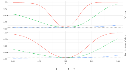
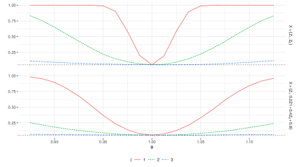
400	6.26	5.90	5.82	6.62	6.60	6.52
600	5.82	4.98	5.30	6.46	5.34	5.06
800	5.82	5.20	4.98	5.98	5.60	5.36
Wald
400	13.18	8.54	3.88	13.78	8.28	4.18
600	10.42	6.66	2.32	12.22	7.22	2.50
800	10.40	6.72	1.26	11.94	6.78	1.26

• Notes: Based on 5000 Monte carlo replications. The $Z_{k}\sim U(-3/2,3/2)$ are independently drawn.

Figure 3: ERF (%) $\epsilon\sim\mathcal{N}(0,1)$, index function as in (S35), $X=(Z_{1},Z_{2})$

Based on 5000 Monte carlo replications. The $Z_{k}\sim U(-3/2,3/2)$ are independently drawn.

Table 8: Index functions used in the simulation exeriments

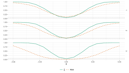
name	expression	$c_{1}$	$c_{2}$	$c_{3}$
Exponential	$\pi_{j}(z)=5\exp(-z^{2}/2c_{j}^{2})$	1.250	2.000	4.00
Logistic	$\pi_{j}(z)=25(1+\exp(-z/c_{j}))^{-1}$	0.296	2.667	24.00
Linear	$\pi_{j}(z)=c_{j}z$	1.000	0.300	0.09

• The $c_{j}$ for the logistic functions correspond to $c_{j}=72/3^{(7-2j)}$.

Table 9: Empirical rejection frequencies, IV, Design 1

		$\hat{S}$				AR	TSLS W	GMM W	GMM LM
$n$	$j$	OLS	$k=6$	AIC	BIC
Exponential
200	1	0.74	5.78	5.78	5.70	4.98	4.94	8.04	5.56
200	2	0.24	6.16	6.16	6.20	4.98	12.20	13.58	6.10
200	3	0.04	6.14	6.14	6.38	4.98	30.36	58.44	19.48
400	1	0.12	5.18	5.18	5.08	5.30	4.86	6.24	5.32
400	2	0.02	5.74	5.74	5.60	5.30	11.36	8.66	5.30
400	3	0.00	3.18	3.18	3.72	5.30	30.72	35.98	12.92
600	1	0.04	5.30	5.30	5.30	5.36	5.40	6.00	5.32
600	2	0.00	5.50	5.50	5.40	5.36	12.18	7.54	5.70
600	3	0.00	2.14	2.14	2.64	5.36	30.92	28.02	10.94
Logistic
200	1	4.74	5.00	5.00	4.52	4.98	4.94	4.92	5.20
200	2	4.74	4.74	4.74	4.78	4.98	4.98	5.64	5.36
200	3	2.24	6.80	6.80	6.92	4.98	7.76	40.42	15.24
400	1	5.18	4.86	4.60	4.54	5.30	5.36	5.10	4.98
400	2	5.18	5.04	5.04	5.00	5.30	5.10	5.50	5.24
400	3	2.28	4.26	4.26	4.62	5.30	5.92	23.88	10.52
600	1	5.34	5.46	5.30	4.76	5.36	5.28	5.14	5.60
600	2	5.34	5.46	5.46	5.44	5.36	5.54	6.00	5.48
600	3	2.68	3.68	3.68	3.92	5.36	6.30	18.82	9.42
Linear
200	1	4.74	5.32	5.32	5.50	4.98	4.64	8.56	5.60
200	2	2.28	7.04	7.04	7.06	4.98	6.88	33.46	12.68
200	3	0.14	4.66	4.66	5.28	4.98	15.12	89.54	46.52
400	1	5.18	5.32	5.32	5.32	5.30	5.16	6.52	5.44
400	2	2.36	5.08	5.08	5.18	5.30	5.42	19.74	8.88
400	3	0.02	1.12	1.12	2.08	5.30	10.92	78.72	37.06
600	1	5.34	5.58	5.58	5.62	5.36	5.42	7.00	6.18
600	2	2.86	4.30	4.30	4.62	5.36	6.08	15.52	8.58
600	3	0.00	0.28	0.28	0.66	5.36	10.68	69.00	31.44

• Notes: Based on 5000 Monte carlo replications. All $\hat{S}$ tests except “OLS” use Legendre polynomials to estimate $\pi$.

Figure 4: $\pi_{j}(z)=5\exp(-z^{2}/2c_{j}^{2})$

Figure 5: $\pi_{j}(z)=25(1+\exp(-z/c_{j}))^{-1}$

Figure 6: $\pi_{j}(z)=c_{j}z$

Table 10: Empirical rejection frequencies, IV, Design 2, $\pi_{1,j}=\pi_{2,j}$

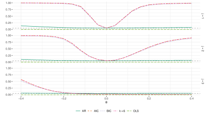
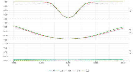
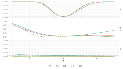
		$\hat{S}$				AR	TSLS W	GMM W	GMM LM
$n$	$j$	OLS	$k=3$	AIC	BIC
Exponential
200	1	3.62	4.88	4.80	4.90	5.28	3.94	21.40	9.32
200	2	2.28	5.44	5.40	5.14	5.28	13.16	49.92	17.62
200	3	0.92	5.50	5.46	5.06	5.28	36.94	99.40	76.08
400	1	0.64	4.82	4.82	4.64	5.20	3.84	13.22	7.16
400	2	0.14	4.96	4.96	4.82	5.20	12.12	27.84	12.14
400	3	0.02	6.48	6.48	5.68	5.20	35.00	95.40	59.42
600	1	0.22	4.64	4.64	4.80	5.34	4.04	9.48	6.24
600	2	0.00	5.04	5.04	5.08	5.34	13.04	19.12	9.08
600	3	0.00	6.34	6.34	6.24	5.34	36.68	88.00	48.02
Logistic
200	1	5.06	4.56	1.86	2.42	5.28	5.40	6.22	5.46
200	2	5.06	4.52	4.56	4.56	5.28	5.50	9.06	5.92
200	3	4.56	5.16	5.14	4.84	5.28	8.72	95.36	60.26
400	1	5.00	5.14	3.34	3.12	5.20	5.30	5.98	5.58
400	2	5.00	4.78	4.78	4.80	5.20	5.40	6.58	5.64
400	3	4.52	6.16	6.16	5.80	5.20	7.42	79.14	42.14
600	1	5.04	4.40	3.64	3.32	5.34	5.30	5.24	5.16
600	2	5.04	4.82	4.82	4.54	5.34	5.10	6.40	5.20
600	3	4.12	5.94	5.94	5.62	5.34	6.94	63.94	32.82
Linear
200	1	5.06	4.92	4.90	4.68	5.28	5.28	20.86	9.42
200	2	4.14	5.02	4.98	4.80	5.28	8.28	90.42	49.82
200	3	2.38	5.74	5.78	5.34	5.28	15.28	99.98	95.46
400	1	5.00	5.04	5.04	4.68	5.20	5.30	12.34	7.38
400	2	4.30	5.78	5.78	5.60	5.20	6.94	68.50	34.12
400	3	0.34	6.92	6.92	6.20	5.20	12.16	99.96	91.84
600	1	5.04	4.98	4.98	4.72	5.34	5.22	10.08	6.88
600	2	3.86	5.58	5.58	5.30	5.34	6.52	53.24	26.44
600	3	0.00	6.04	6.04	5.58	5.34	11.34	99.78	88.42

• Notes: Based on 2500 Monte carlo replications. $k=3$ indicates that each univariate series forming the tensor series has $k=3$.

Table 11: Empirical rejection frequencies, IV, Design 2, $\pi_{2,j}=c_{j}Z_{2,2}$

		$\hat{S}$				AR	TSLS W	GMM W	GMM LM
$n$	$j$	OLS	$k=3$	AIC	BIC
Exponential
200	1	4.88	4.74	4.68	4.66	5.28	5.10	24.60	11.38
200	2	4.14	5.54	5.44	4.90	5.28	12.00	85.52	44.02
200	3	1.40	5.24	5.22	4.94	5.28	29.20	99.94	92.38
400	1	5.26	4.98	4.98	4.96	5.20	4.76	15.06	8.42
400	2	3.70	5.62	5.62	5.36	5.20	11.30	61.32	28.94
400	3	0.06	6.56	6.56	5.88	5.20	26.64	99.68	86.80
600	1	4.84	4.64	4.64	4.22	5.34	5.02	11.64	7.10
600	2	3.48	5.64	5.64	5.40	5.34	11.72	47.58	23.32
600	3	0.00	6.40	6.40	5.80	5.34	27.80	99.22	82.16
Logistic
200	1	5.06	4.80	3.38	3.64	5.28	5.26	17.16	8.88
200	2	5.62	5.54	5.58	5.28	5.28	7.88	78.96	39.44
200	3	4.52	5.30	5.30	5.04	5.28	14.74	99.80	86.88
400	1	5.00	5.22	4.40	4.12	5.20	5.14	10.62	7.22
400	2	5.80	5.90	5.90	5.70	5.20	6.70	54.62	25.14
400	3	4.00	6.28	6.28	5.94	5.20	11.84	99.04	80.50
600	1	5.04	4.68	4.22	3.86	5.34	5.24	9.10	6.42
600	2	5.92	5.26	5.26	4.96	5.34	6.24	42.44	21.60
600	3	3.72	6.32	6.32	5.88	5.34	11.34	97.44	74.64
Linear
200	1	5.06	4.92	4.90	4.68	5.28	5.28	20.86	9.42
200	2	4.14	5.02	4.98	4.80	5.28	8.28	90.42	49.82
200	3	2.38	5.74	5.78	5.34	5.28	15.28	99.98	95.46
400	1	5.00	5.04	5.04	4.68	5.20	5.30	12.34	7.38
400	2	4.30	5.78	5.78	5.60	5.20	6.94	68.50	34.12
400	3	0.34	6.92	6.92	6.20	5.20	12.16	99.96	91.84
600	1	5.04	4.98	4.98	4.72	5.34	5.22	10.08	6.88
600	2	3.86	5.58	5.58	5.30	5.34	6.52	53.24	26.44
600	3	0.00	6.04	6.04	5.58	5.34	11.34	99.78	88.42

• Notes: Based on 2500 Monte carlo replications. $k=3$ indicates that each univariate series forming the tensor series has $k=3$.

Figure 7: $\pi_{i}$ exponential with $j=1$ $(i=1,2)$

(a) AR

(b) $\hat{S}$ ($k=3$)

Figure 8: $\pi_{1}$ exponential with $j=1$, $\pi_{2}$ exponential with $j=3$

(a) AR

(b) $\hat{S}$ ($k=3$)

Figure 9: $\pi_{1}$ exponential with $j=3$, $\pi_{2}$ exponential with $j=3$

(a) AR

(b) $\hat{S}$ ($k=3$)

Figure 10: $\pi_{i}$ logistic with $j=1$ $(i=1,2)$

(a) AR

(b) $\hat{S}$ ($k=3$)

Figure 11: $\pi_{1}$ logistic with $j=1$, $\pi_{2}$ logistic with $j=3$

(a) AR

(b) $\hat{S}$ ($k=3$)

Figure 12: $\pi_{1}$ logistic with $j=3$, $\pi_{2}$ logistic with $j=3$

(a) AR

(b) $\hat{S}$ ($k=3$)

Figure 13: $\pi_{i}$ linear with $j=1$ $(i=1,2)$

(a) AR

(b) $\hat{S}$ ($k=3$)

Figure 14: $\pi_{1}$ linear with $j=1$, $\pi_{2}$ linear with $j=3$

(a) AR

(b) $\hat{S}$ ($k=3$)

Figure 15: $\pi_{1}$ linear with $j=3$, $\pi_{2}$ linear with $j=3$

(a) AR

(b) $\hat{S}$ ($k=3$)

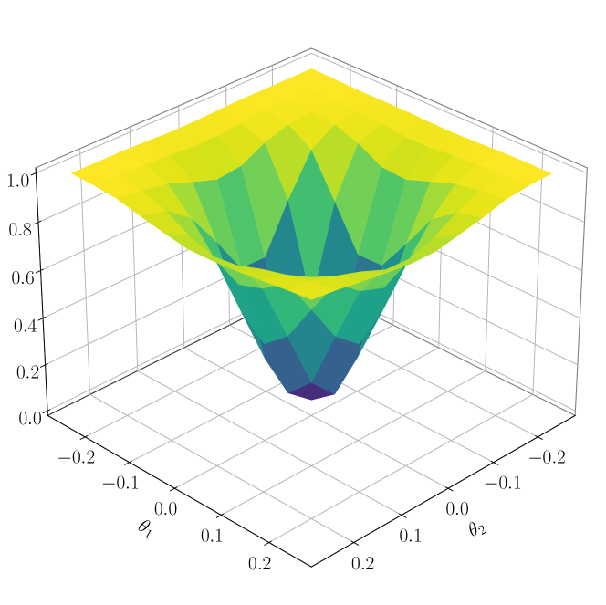
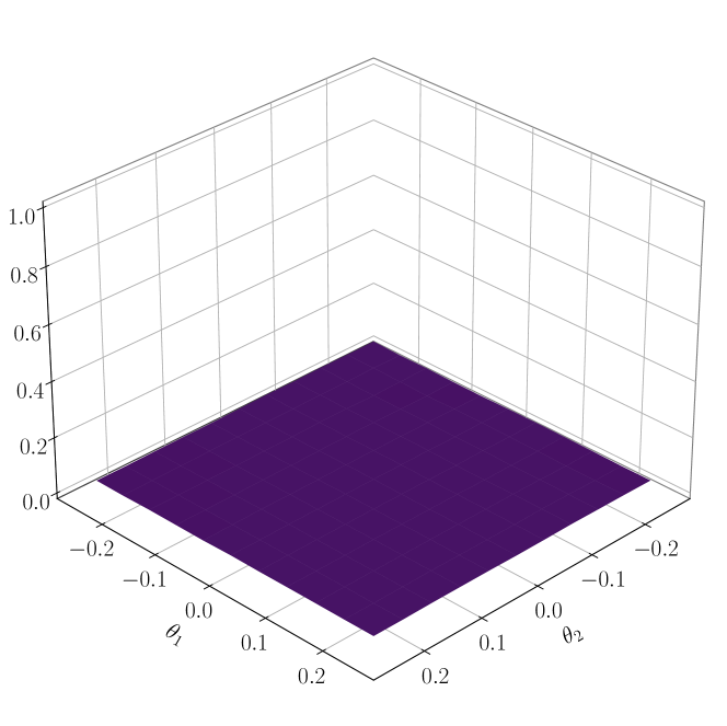
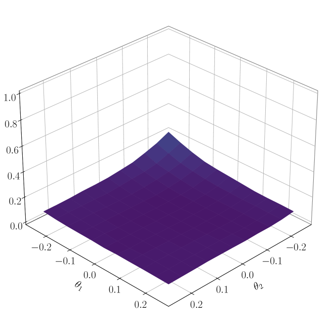
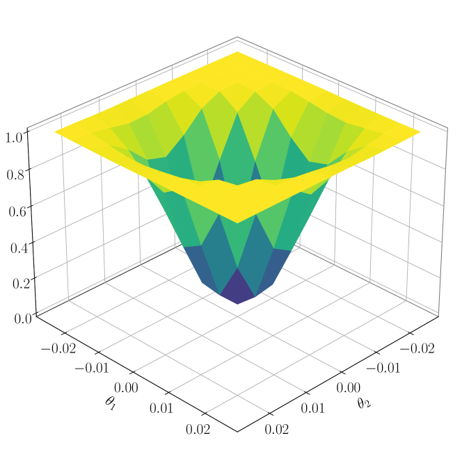
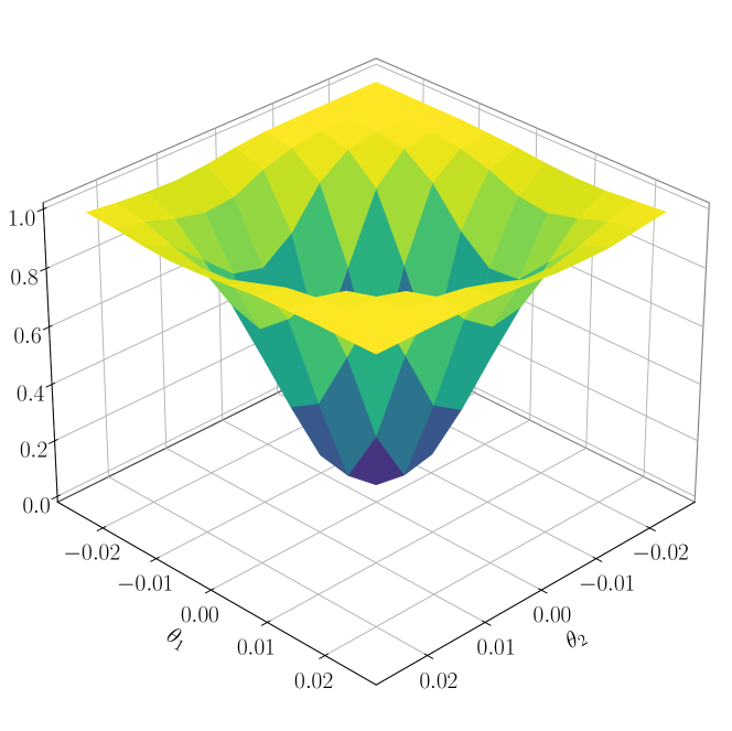
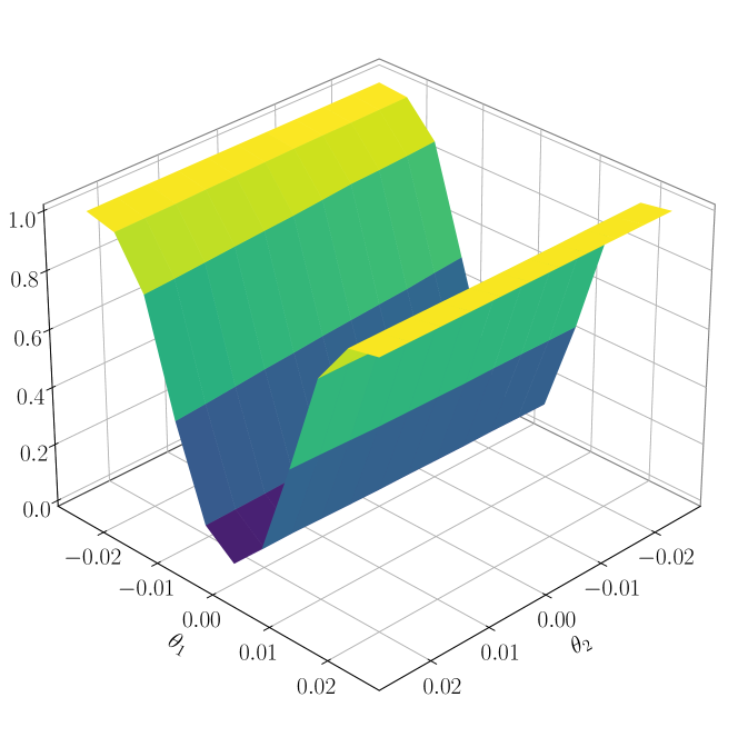
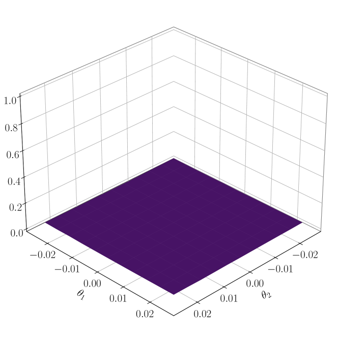
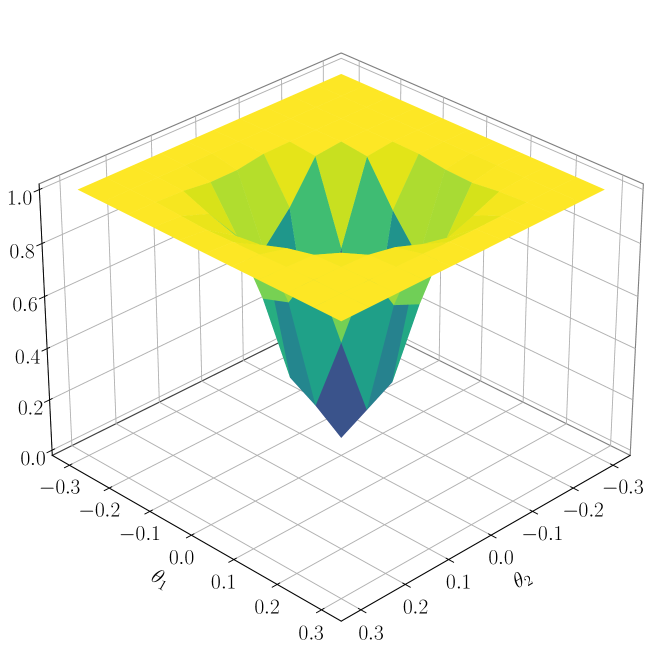
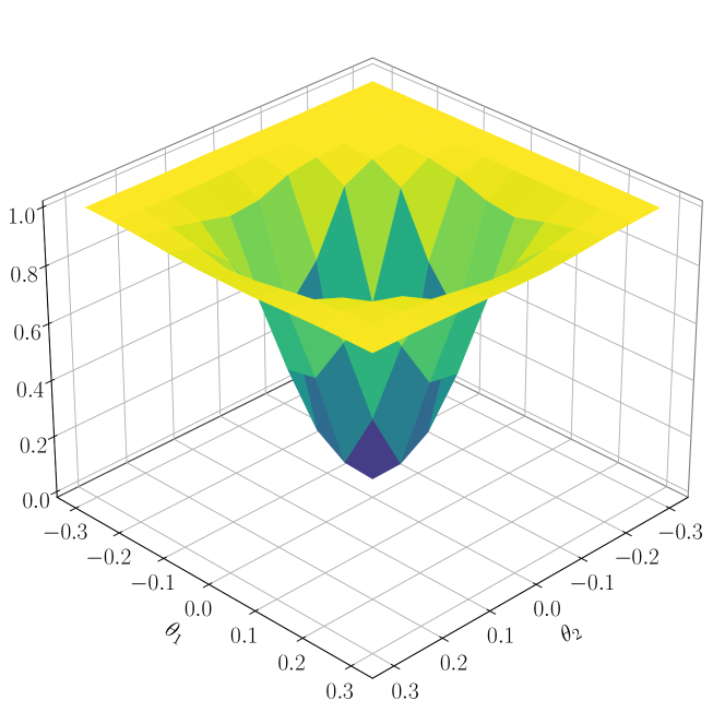
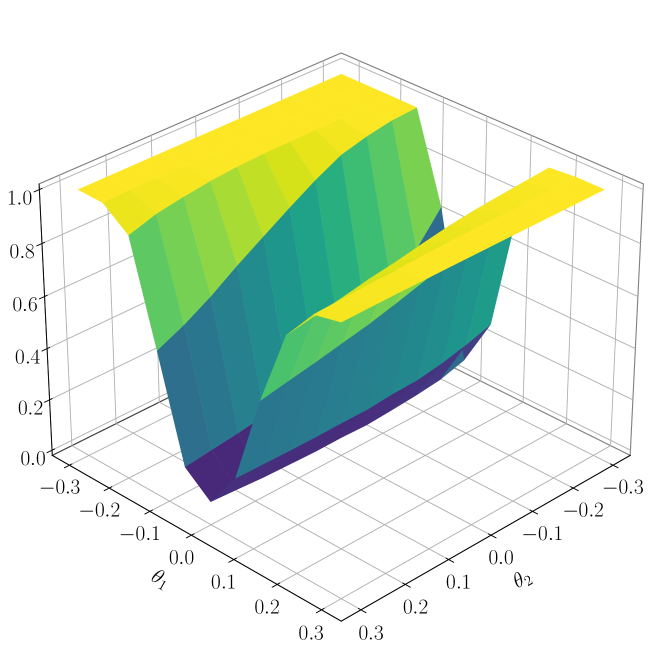
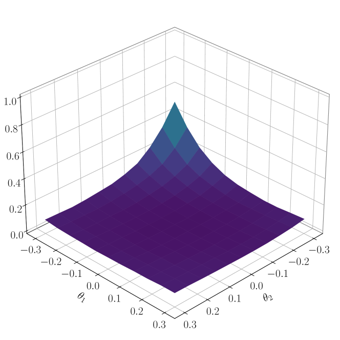
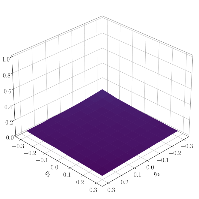
Supplementary material for “Locally regular and efficient tests in non-regular semiparametric models”

Adam LeeBI Norwegian Business School, adam.lee@bi.no.

Appendix S1 Notation

$x\coloneqq y$ means that $x$ is defined to be $y$. The Lebesgue measure on $\mathbb{R}^{K}$ is denoted by $\lambda_{K}$ or $\lambda$ if the dimension is clear from context. The standard basis vectors in $\mathbb{R}^{K}$ are $e_{1},\ldots,e_{K}$. For any matrix $M$, $M^{\dagger}$ is its Moore – Penrose pseudoinverse. We make use of the empirical process notation: $Pf\coloneqq\int f\,\mathrm{d}P$, $\mathbb{P}_{n}f\coloneqq\frac{1}{n}\sum_{i=1}^{n}f(Y_{i})$ and $\mathbb{G}_{n}f\coloneqq\sqrt{n}(\mathbb{P}_{n}-P)f$. For any two sequence of probability measures $(Q_{n})_{n\in\mathbb{N}}$ and $(P_{n})_{n\in\mathbb{N}}$ (where $Q_{n}$ and $P_{n}$ are defined on a common measurable space for each $n\in\mathbb{N}$), $Q_{n}\triangleleft P_{n}$ indicates that $(Q_{n})_{n\in\mathbb{N}}$ is contiguous with respect to $(P_{n})_{n\in\mathbb{N}}$. $Q_{n}\triangleleft\triangleright\;P_{n}$ indicates that both $Q_{n}\triangleleft P_{n}$ and $P_{n}\triangleleft Q_{n}$ hold, see van der Vaart (1998, Section 6.2) for formal definitions. $X\mathchoice{\mathrel{\hbox to0.0pt{$\displaystyle\perp$\hss}\mkern 2.0mu{\displaystyle\perp}}}{\mathrel{\hbox to0.0pt{$\textstyle\perp$\hss}\mkern 2.0mu{\textstyle\perp}}}{\mathrel{\hbox to0.0pt{$\scriptstyle\perp$\hss}\mkern 2.0mu{\scriptstyle\perp}}}{\mathrel{\hbox to0.0pt{$\scriptscriptstyle\perp$\hss}\mkern 2.0mu{\scriptscriptstyle\perp}}}Y$ indicates that random vectors $X$ and $Y$ are independent; $X\simeq Y$ indicates that they have the same distribution. $a\lesssim b$ means that $a$ is bounded above by $Cb$ for some constant $C\in(0,\infty)$; the constant $C$ may change from line to line. $\operatorname{cl}X$ means the closure of $X$. If $S$ is a subset of a vector space, $\operatorname{lin}S$ or $\operatorname{Span}S$ means the linear span of $S$. If $S$ is a subset of a topological vector space, $\overline{\operatorname{lin}}\ S$ or $\operatorname{cl}\operatorname{Span}S$ means the closure of the linear span of $S$. If $S$ is a subset of an inner product space $(V,\left\langle{\cdot}\,,\,{\cdot}\right\rangle)$, $S^{\perp}$ is its orthogonal complement, i.e. $S^{\perp}=\{x\in V:\left\langle{x}\,,\,{s}\right\rangle=0\text{ for all }s\in S\}$. If $S\subset V$ is complete (hence a Hilbert space) the orthogonal projection of $x\in V$ onto $S$ is $\Pi(x|S)$. The total variation distance between measures $P$ and $Q$ defined on the measurable space $(\Omega,\mathcal{F})$ is $d_{TV}(P,Q)=\sup_{A\in\mathcal{F}}|P(A)-Q(A)|$. $\overset{P_{n}}{\rightsquigarrow}$ denotes weak convergence under the sequence of measures $P_{n}$. If the sequence of measures is clear from context, I write just $\rightsquigarrow$.

Appendix S2 Additional results

S2.1 A consistent estimator of the Moore – Penrose pseudoinverse

As is well known, the Moore – Penrose pseudoinverse of a matrix is not a continuous function on the space of positive semi-definite matrices (see e.g. Ben-Israel and Greville, 2003, Section 6.6). In consequence, if one has a consistent estimator $\check{M}_{n}$ of some matrix $M$, it need not follow that $\check{M}^{\dagger}$ is consistent for $M^{\dagger}$. A necessary and sufficient condition for this convergence in probability to occur is that $\operatorname{rank}(\check{M}_{n})=\operatorname{rank}(M)$ with probability approaching one as $n\to\infty$ (Andrews, 1987, Theorem 2).

Here I record a construction given in the supplementary appendix to Lee and Mesters (2024a) which results in an estimator $\hat{M}_{n}$ which is consistent for $M$ and satisfies $\operatorname{rank}{\hat{M}_{n}}=\operatorname{rank}{M}$ with probability approaching one as $n\to\infty$ and, in consequence, $\hat{M}_{n}^{\dagger}$ is consistent for $M^{\dagger}$. This construction requires an initial estimator with a known rate of convergence and is based on a spectral cut-off regularisation scheme. It is very similar to that considered in Lütkepohl and Burda (1997) and is a special case of the larger class of regularisation schemes considered by Dufour and Valéry (2016). That this results in an estimator with the claimed properties is recorded in Proposition S1 below, which is proven in Lee and Mesters (2024b).

In particular, suppose that the sequence of (random) positive semi-definite (symmetric) matrices $(\check{M}_{n})_{n\in\mathbb{N}}$ (of fixed dimension $L\times L$) satisfy

$$P_{n}\left(\|\check{M}_{n}-M_{n}\|_{2}<\upnu_{n}\right)\to 1,$$ (S1)

for a sequence $(P_{n})_{n\in\mathbb{N}}$ of probability measures, a known non-negative sequence $\upnu_{n}\to 0$ and a sequence of deterministic matrices $M_{n}\to M$ with $\operatorname{rank}(M_{n})=\operatorname{rank}(M)$ for all sufficiently large $n$. Let $\check{M}_{n}=\check{U}_{n}\check{\Lambda}_{n}\check{U}_{n}^{\prime}$ be the corresponding eigendecompositions and define

$$\hat{M}_{n}\coloneqq\check{U}_{n}\Lambda_{n}(\upnu_{n})\check{U}^{\prime}_{n}~{},$$ (S2)

where $\Lambda_{n}(\upnu_{n})$ is a diagonal matrix with the $\upnu_{n}$-truncated eigenvalues of $\check{M}_{n}$ on the main diagonal and $\check{U}_{n}$ is the matrix of corresponding orthonormal eigenvectors. That is, if $(\check{\lambda}_{n,i})_{i=1}^{L}$ denote the non-increasing eigenvalues of $\check{M}_{n}$, then the $(i,i)$-th element of $\Lambda_{n}(\upnu_{n})$ is $\check{\lambda}_{n,i}\bm{1}(\check{\lambda}_{n,i}\geq\upnu_{n})$.

Proposition S1 (Proposition S1 in Lee and Mesters (2024a)):

If (S1) holds, $M_{n}\to M$ and for all $n$ greater than some $N\in\mathbb{N}$ $\operatorname{rank}(M_{n})=\operatorname{rank}(M)$, then $\hat{M}_{n}\xrightarrow[]{P_{n}}M$ and

$$P_{n}\left(\operatorname{rank}(\hat{M}_{n})=\operatorname{rank}(M)\right)\to 1,$$

where $\hat{M}_{n}$ is defined as in (S2). In consequence,

$$\hat{M}_{n}^{\dagger}\xrightarrow{P_{n}}M^{\dagger}.$$

S2.2 The quotient space $\mathbb{H}_{\gamma}$

I first briefly recall some preliminaries regarding quotient spaces, for the convenience of the reader. Following this a lemma used during the development of the power bounds is established.

S2.2.1 Preliminaries on quotient spaces

Let $X$ be a linear space and $V$ a subspace of $X$. The quotient of $X$ by $V$, ${X}\,/\,{V}$ is a linear space whose elements are the cosets $[x]\coloneqq x+V\coloneqq\{x+n:n\in V\}$ (for $x\in X$). $x$ (or any other member of $[x]$) is a coset representative. The zero vector in ${X}\,/\,{V}$ is $[0]=0+V=V$.

Vector addition and scalar multiplication are defined according to:

$$[x+y]\coloneqq[x]+[y],\quad[ax]\coloneqq a[x]\quad\text{ for all }[x],[y]\in{X}\,/\,{V}\text{ and all }a\in\mathbb{R}.$$

The map $\pi_{V}:X\to{X}\,/\,{V}$ defined by $\pi_{V}(x)\coloneqq[x]$ is the natural projection or quotient map. $\pi_{V}$ is a surjective linear transformation with $\ker\pi_{N}=V$ (Roman, 2005, Theorem 3.2).

There are two main cases of interest in the present paper. In the first, $X$ is a linear space equipped with a positive semi-definite symmetric bilinear form, $\left\langle{\cdot}\,,\,{\cdot}\right\rangle$. Let $\|\cdot\|$ be the corresponding semi-norm formed in the usual way: $\|x\|\coloneqq\sqrt{\left\langle{x}\,,\,{x}\right\rangle}$ and let $V\coloneqq\{x\in X:\|x\|=0\}$, which is evidently a subspace of $X$. We define an inner product on ${X}\,/\,{V}$ as follows:

$$\left\langle{[x]}\,,\,{[y]}\right\rangle_{V}\coloneqq\left\langle{x}\,,\,{y}\right\rangle.$$

Symmetry and linearity in the first argument of $\left\langle{\cdot}\,,\,{\cdot}\right\rangle_{V}$ follow from the corresponding properties of $\left\langle{\cdot}\,,\,{\cdot}\right\rangle$. For positive definiteness, suppose that $[x]\neq[0]$. Then, $\left\langle{x}\,,\,{x}\right\rangle_{V}=\|x\|^{2}>0$ since $x\notin\ker\pi_{V}=V$. In consequence $({X}\,/\,{V},\,\left\langle{\cdot}\,,\,{\cdot}\right\rangle_{V})$ is an inner product (pre-Hilbert) space. The induced norm on ${X}\,/\,{V}$ evidently satisfies $\|[x]\|_{V}=\|\pi_{V}(x)\|_{V}=\|x\|$.

In the second case of interest, $X$ is a linear space equipped with a semi-norm $\|\cdot\|$. Let $V\coloneqq\{x\in X:\|x\|=0\}$, which is evidently a subspace of $X$. We define a norm on ${X}\,/\,{V}$ as follows:

$$\|[x]\|_{V}\coloneqq\|x\|.$$

This definition ensures that $({X}\,/\,{V},\|\cdot\|_{V})$ is a normed space (Rudin, 1991, 1.43).

S2.2.2 A lemma on the kernel of $\pi_{1}$

Lemma S1:

Suppose Assumption 1 holds and $B_{\eta}$ is a linear space. Let $\pi_{1}^{\prime}$ denote the restriction of $\pi_{1}$ to $\mathbb{H}_{\gamma}$. Then, the closure of $\ker\pi_{1}^{\prime}$ in $\overline{\mathbb{H}_{\gamma}}$ is $\ker\pi_{1}$.

Proof.

Since $\pi_{1}$ is continuous, $\ker\pi_{1}=\pi_{1}^{-1}(\{0\})$ is closed. Hence it suffices to show that

$$\ker\pi_{1}=\{[h]\in\overline{\mathbb{H}_{\gamma}}:[h]=[0,b]\}\subset\operatorname{cl}\ker\pi_{1}^{\prime}=\operatorname{cl}\{[h]\in\mathbb{H}_{\gamma}:[h]=[0,b]\}.$$

Let $[h]=[0,b]\in\ker\pi_{1}$. There is a sequence $\mathbb{H}_{\gamma}\ni[h_{n}]=[t_{n},b_{n}]\to[h]$. Decomposing the norm, we have that

$$\|[h_{n}]-[h]\|_{\gamma} =\|\Pi^{\perp}[h_{n}]-\Pi^{\perp}[h]_{\gamma}\|_{\gamma}+\Pi[h_{n}]-\Pi[h]\|_{\gamma}$$

$$=t_{n}^{\prime}\tilde{\mathcal{I}}_{\gamma}t_{n}+\|\Pi[t_{n},0]+[0,b_{n}]-[0,b]\|_{\gamma}$$

$$=t_{n}^{\prime}\tilde{\mathcal{I}}_{\gamma}t_{n}+\left\|\sum_{j=1}^{d_{\theta}}t_{n,j}\Pi[e_{j},0]+[0,b_{n}]-[0,b]\right\|_{\gamma}$$

$$=t_{n}^{\prime}\tilde{\mathcal{I}}_{\gamma}t_{n}+\left\|t_{n}^{\prime}\bm{e}+[0,b_{n}]-[0,b]\right\|_{\gamma},$$

with $\bm{e}=(\Pi[e_{1},0],\ldots,\Pi[e_{d_{\theta}},0])^{\prime}$, where $e_{j}$ is the $j$-th canonical basis vector in $\mathbb{R}^{d_{\theta}}$. For each $n\in\mathbb{N}$, there are $\check{\bm{e}}_{n}=([0,\check{b}_{1,n}],\ldots,[0,\check{b}_{d_{\theta},n}])^{\prime}$ with each $[0,\check{b}_{j,n}]\in\mathbb{H}_{\gamma}$ such that

$$\left\|[0,\check{b}_{j,n}]-\Pi[e_{j},0]\right\|\leq\frac{1}{n|t_{n,j}|}.$$

Hence, putting $[0,\tilde{b}_{n}]\coloneqq t_{n}^{\prime}\check{\bm{e}}_{n}+[0,b_{n}]$, we have

$$\|[0,\tilde{b}_{n}]-[0,b]\|_{\gamma}\leq\|t_{n}^{\prime}\check{\bm{e}}_{n}-t_{n}^{\prime}\bm{e}\|_{\gamma}+\|t_{n}^{\prime}\bm{e}+[0,b_{n}]-[0,b]\|_{\gamma}\leq\frac{d_{\theta}}{n}+o(1)=o(1).$$

Since each $[0,\tilde{b}_{n}]\in\ker\pi_{1}^{\prime}$, the limit $[0,b]\in\operatorname{cl}\ker\pi_{1}^{\prime}$. ∎

S2.3 Uniform Local Asymptotic Normality

The equivalence discussed in Remark 2 is proved in Proposition S2 below, which is an adaptation of Theorem 80.13 in Strasser (1985). $H_{\gamma}$ is assumed to be a subset (containing 0) of a linear space equipped with some pseudometric.

Assumption S1 (Uniform local asymptotic normality):

$L_{n,\gamma}(h)$ satisfies

$$L_{n,\gamma}(h)=\Delta_{n,\gamma}h-\frac{1}{2}\|\Delta_{n,\gamma}h\|^{2}+R_{n,\gamma}(h),$$

where $h=(\tau,b)$, $\Delta_{n,\gamma}:\overline{\operatorname{lin}}\ H_{\gamma}\to L_{2}^{0}(P_{n,\gamma})$ are bounded linear maps and for any $h_{n}\to h$ in $H_{\gamma}$, $R_{n}(\gamma,h_{n})\xrightarrow{P_{n,\gamma}}0$. Additionally, suppose that for each $h_{n}\to h$ in $H_{\gamma}$, $(\Delta_{n,\gamma}h_{n})_{n\in\mathbb{N}}$ is uniformly square $P_{n,\gamma}$-integrable and

$$\left(\Delta_{n,\gamma}h_{n},\Delta_{n,\gamma}h\right)^{\prime}\overset{P_{n,\gamma}}{\rightsquigarrow}\mathcal{N}\left(0,\sigma_{\gamma}(h)\left[\begin{smallmatrix}1&1\\ 1&1\end{smallmatrix}\right]\right),\qquad\sigma_{\gamma}(h)\coloneqq\lim_{n\to\infty}\|\Delta_{n,\gamma}h\|^{2}.$$

Remark 1:

Assumption S1 ensures that the pairs of sequences $(P_{n,\gamma})_{n\in\mathbb{N}}$ and $(P_{n,\gamma,h_{n}})_{n\in\mathbb{N}}$ are mutually contiguous for any $h_{n}\to h\in H_{\gamma}$ (see e.g. van der Vaart, 1998, Example 6.5).

Remark 2:

In Assumption S1, the assumption of joint convergence of $(\Delta_{n}h_{n},\Delta_{n}h)^{\prime}$ is nedeed only because $H_{\gamma}$ is not required to be linear. If $H_{\gamma}$ is a linear space this follows from the Cramér – Wold Theorem given the definition of $\sigma_{\gamma}(h)$.

Remark 3:

If $(\Delta_{n,\gamma})_{n\in\mathbb{N}}$ is asymptotically equicontinuous on compact subsets $K\subset H_{\gamma}$, then $h_{n}\to h$ in $H_{\gamma}$ implies $\|\Delta_{n,\gamma}(h_{n}-h)\|\to 0$. In consequence $(\Delta_{n,\gamma}h)_{n\in\mathbb{N}}$ being uniformly square $P_{n,\gamma}$-integrable and $\Delta_{n,\gamma}h\overset{P_{n,\gamma}}{\rightsquigarrow}\mathcal{N}(0,\sigma_{\gamma}(h))$ for each $h\in H_{\gamma}$, suffices for $(\Delta_{n,\gamma}h_{n})_{n\in\mathbb{N}}$ being uniformly square $P_{n,\gamma}$-integrable and

$$\left(\Delta_{n,\gamma}h_{n},\ \Delta_{n,\gamma}h\right)^{\prime} =\begin{pmatrix}1&1\\ 0&1\end{pmatrix}\left(\Delta_{n,\gamma}h_{n}-\Delta_{n,\gamma}h,\ \Delta_{n,\gamma}h\right)^{\prime}$$

$$\overset{P_{n,\gamma}}{\rightsquigarrow}\mathcal{N}\left(0,\left[\begin{smallmatrix}1&1\\ 0&1\end{smallmatrix}\right]\left[\begin{smallmatrix}0&0\\ 0&\sigma_{\gamma}(h)\end{smallmatrix}\right]\left[\begin{smallmatrix}1&1\\ 0&1\end{smallmatrix}\right]^{\prime}\right)$$

$$\;\;\;=\mathcal{N}\left(0,\sigma_{\gamma}(h)\left[\begin{smallmatrix}1&1\\ 1&1\end{smallmatrix}\right]\right),$$

for any $h_{n}\to h\in H_{\gamma}$.

If $H_{\gamma}$ is a Banach space metrised by its norm, the equicontinuity of $(\Delta_{n,\gamma})_{n\in\mathbb{N}}$ is guaranteed as uniform boundedness of $(\Delta_{n,\gamma})_{n\in\mathbb{N}}$ (hence equicontinuity on $H_{\gamma}$) is implied by uniform square $P_{n,\gamma}$-integrability of $(\Delta_{n,\gamma}h)_{n\in\mathbb{N}}$ for $h\in H_{\gamma}$.

Proposition S2:

Assumption S1 is equivalent to Assumption 1 plus asymptotic equicontinuity on compact subsets $K\subset H_{\gamma}$ of $(\Delta_{n,\gamma})_{n\in\mathbb{N}}$ and $(h\mapsto P_{n,\gamma,h})_{n\in\mathbb{N}}$, where the metric on the relevant space of probability measures is $d_{TV}$.

Proof.

Suppose first that Assumption 1 and the asymptotic equicontinuity conditions hold. Let $h_{n}\to h$ in $H_{\gamma}$. By asymptotic equicontinuity of $(h\mapsto P_{n,\gamma,h})_{n\in\mathbb{N}}$,

$$\lim_{n\to\infty}d_{TV}(P_{n,\gamma,h_{n}},P_{n,\gamma,h})=0\quad\Longrightarrow\quad\lim_{n\to\infty}\int\left|\frac{p_{n,\gamma,h_{n}}}{p_{n,\gamma,0}}-\frac{p_{n,\gamma,h}}{p_{n,\gamma,0}}\right|\,\mathrm{d}P_{n,\gamma,0}=0.$$

In combination with (compact) asymptotic equicontinuity of $(\Delta_{n,\gamma})_{n\in\mathbb{N}}$, this yields

$$R_{n,\gamma}(h_{n})-R_{n,\gamma}(h)=L_{n,\gamma}(h_{n})-L_{n,\gamma}(h)+o_{P_{n,\gamma}}(1)=o_{P_{n,\gamma}}(1).$$

That $(\Delta_{n,\gamma}h_{n})_{n\in\mathbb{N}}$ is uniformly square $P_{n,\gamma}$-integrable and the required joint weak convergence under $P_{n,\gamma}$ follows from the asymptotic equicontinuity of $(\Delta_{n,\gamma})_{n\in\mathbb{N}}$ on compacts as discussed in Remark 3.

For the converse suppose that Assumption S1 holds. We need to prove only the asymptotic equicontinuity conditions. It suffices to show that (i) $\|\Delta_{n,\gamma}(h_{n}-h)\|\to 0$ and (ii) $d_{TV}(P_{n,\gamma,h_{n}},P_{n,\gamma,h})$ for any $h_{n}\to h$ with $h_{n},h\in K\subset H_{\gamma}$. (i) holds since for any convergent $h_{n}\to h\in H_{\gamma}$ we have $\Delta_{n,\gamma}(h_{n}-h)=(1,-1)(\Delta_{n,\gamma}h_{n},\Delta_{n,\gamma}h)^{\prime}\xrightarrow{P_{n,\gamma}}0$ and so by the square uniform integrability and e.g. Theorem 2.7 in Serfozo (1982), $\|\Delta_{n,\gamma}(h_{n}-h)\|^{2}\to 0$. That (ii) holds follows from Lemma S4 and

$$L_{n,\gamma}(h_{n})-L_{n,\gamma}(h) =\Delta_{n,\gamma}h_{n}-\frac{1}{2}\|\Delta_{n,\gamma}h_{n}\|^{2}+R_{n,\gamma}(h_{n})-\left[\Delta_{n,\gamma}h-\frac{1}{2}\|\Delta_{n,\gamma}h\|^{2}+R_{n,\gamma}(h)\right]$$

$$=o_{P_{n,\gamma}}(1),$$

since $R_{n,\gamma}(h_{n})=o_{P_{n,\gamma}}(1)$, $R_{n,\gamma}(h)=o_{P_{n,\gamma}}(1)$ and $\|\Delta_{n,\gamma}(h_{n}-h)\|^{2}\to 0$. ∎

The following Lemmas provide conditions which can be useful for demonstrating (compact) equicontinuity in the i.i.d. case.

Lemma S2:

If $H_{\gamma}$ is a linear space and $\Delta_{n,\gamma}h=\frac{1}{\sqrt{n}}\sum_{i=1}^{n}A_{\gamma}h$ for some bounded linear map $A_{\gamma}:H_{\gamma}\to L_{2}(P_{\theta})$, then ($h\mapsto\Delta_{n,\gamma}h)_{n\in\mathbb{N}}$ is equicontinuous on compact subsets of $H_{\gamma}$ in $L_{2}(P_{\theta})$.

Proof.

Let $K\subset H_{\gamma}$ be compact and note that for any $h_{n}\to h$ (all in $K$),

$$\|\Delta_{n,\gamma}(h_{n}-h)\|=\left\|\mathbb{G}_{n}A_{\gamma}(h_{n}-h)\right\|=\|A_{\gamma}(h_{n}-h)\|\leq\|A_{\gamma}\|\|h_{n}-h\|\to 0.\qed$$

Lemma S3:

Let $\Gamma,\Gamma^{\prime}$ be subsets of linear spaces, $H$ a subset of a seminormed linear space $H^{\prime}$ and $\mathcal{W}\subset\mathbb{R}^{K}$. Suppose $\mathcal{V}$ is the intersection of a neighbourhood of 0 in $H^{\prime}$ with $H$ and $\varphi:H\mapsto\Gamma^{\prime}$ is a linear map such that $\upgamma+s\varphi(h)\in\Gamma$ for each $s\in[0,1]$, $h\in\mathcal{V}$ and $\upgamma\in\Gamma$. Let $\mathcal{U}\coloneqq\{\gamma+\varphi(h):h\in\mathcal{V}\}$. If

1. For each $\upgamma\in\Gamma$, $P_{\upgamma}$ is a probability measure on $(\mathcal{W},\mathcal{B}(\mathcal{W}))$, dominated by a $\sigma$ – finite measure $\nu$, with corresponding density $p_{\upgamma}$;

2. $t\mapsto\sqrt{p_{\gamma_{\star}+t\varphi(h)}(w)}$ is absolutely continuous on $[0,1]$ for all $\gamma_{\star}\in\mathcal{U}$, $h\in\mathcal{V}$ and $w\in\mathcal{W}$;

3. For all $\gamma_{\star}\in\mathcal{U},\,h\in\mathcal{V}$, $q_{\gamma_{\star},h,s}(w)=\frac{\partial\log p_{\gamma_{\star}+t\varphi(h)}(w)}{\partial t}|_{t=s}$ satisfies

   $$P_{\gamma_{\star}+s\varphi(h)}[q_{\gamma_{\star},h,s}]^{2}\leq m(s)\|h\|^{2},\quad$$

   for $m:[0,1]\to[0,\infty)$ with $\int_{0}^{1}m(s)\,\mathrm{d}s<\infty$.

Then there is an $N$ such that for all $n\geq N$, the functions $h\mapsto P_{n,\gamma,h}\coloneqq P_{\gamma+\varphi(h/\sqrt{n})}^{n}$ are $d_{TV}$–Lipschitz with a common Lipschitz constant. Consequently, $\{h\mapsto P_{n,\gamma,h}:n\geq N\}$ is uniformly equicontinuous in $d_{TV}$.

Proof.

Let $h^{\star}\in H$ and let $\tilde{h}\coloneqq(h^{\star}-h)$. For all large enough $n$, $h/\sqrt{n}$ and $\tilde{h}/\sqrt{n}$ belong to $\mathcal{V}$ and hence also $\gamma_{0,n}\coloneqq\gamma+\varphi(h/\sqrt{n})\in\mathcal{U}$. Therefore, by (ii) $q_{\gamma_{0,n},\tilde{h}/\sqrt{n},s}(w)$ exists for almost every $s\in(0,1)$ and

$$\sqrt{p_{\gamma+\varphi(h^{\star}/\sqrt{n})}(w)}-\sqrt{p_{\gamma+\varphi(h/\sqrt{n})}(w)} =\sqrt{p_{\gamma_{0,n}+\varphi(\tilde{h}/\sqrt{n})}(w)}-\sqrt{p_{\gamma_{0,n}}(w)}$$

$$=\frac{1}{2}\int_{0}^{1}q_{\gamma_{0,n},\tilde{h}/\sqrt{n},s}(w)\sqrt{p_{\gamma_{0,n}+s\varphi(\tilde{h}/\sqrt{n})}(w)}\,\mathrm{d}s.$$

By Fubini’s Theorem, Jensen’s inequality and S4,

$$\int\left(\sqrt{p_{\gamma+\varphi(h^{\star}/\sqrt{n})}(w)}-\sqrt{p_{\gamma+\varphi(h/\sqrt{n})}(w)}\right)^{2}\,\mathrm{d}\nu \leq\frac{1}{4}\int\int_{0}^{1}q_{\gamma_{0,n},\tilde{h}/\sqrt{n},s}(w)^{2}p_{\gamma_{0,n}+s\varphi(\tilde{h}/\sqrt{n})}(w)\,\mathrm{d}s\,\mathrm{d}\nu$$

$$=\frac{1}{4}\int_{0}^{1}\int q_{\gamma_{0,n},\tilde{h}/\sqrt{n},s}(w)^{2}p_{\gamma_{0,n}+s\varphi(\tilde{h}/\sqrt{n})}(w)\,\mathrm{d}\nu\,\mathrm{d}s$$

$$\leq\frac{1}{4}\int_{0}^{1}m(s)\frac{\|\tilde{h}\|^{2}}{n}\,\mathrm{d}s$$

$$=\frac{M\|h^{\star}-h\|^{2}}{4n},$$

where $M\coloneqq\int_{0}^{1}m(s)\,\mathrm{d}s$. Therefore, by Lemmas 2.15 and 2.17 of Strasser (1985),

$$d_{TV}(P_{n,\gamma,h^{\star}},P_{n,\gamma,h})\leq\frac{\sqrt{2M}}{2}\|h^{\star}-h\|.\qed$$

S2.4 Convergence of log-likelihood ratios and convergence in total variation

Lemma S4:

Suppose that for $h_{n},g\in H_{\gamma}$, $P_{n,\gamma,g}\triangleleft\,P_{n,\gamma}$ and

$$L_{n,\gamma}(h_{n})-L_{n,\gamma}(g)=o_{P_{n,\gamma}}(1).$$

Then $d_{TV}(P_{n,\gamma,h_{n}},P_{n,\gamma,g})\to 0$.

Proof.

By the continuous mapping theorem and Le Cam’s first lemma (e.g. van der Vaart, 1998, Lemma 6.4),

$$\frac{p_{n,\gamma,h_{n}}}{p_{n,\gamma,g}}=\exp\left(L_{n,\gamma}(h_{n})-L_{n,\gamma}(g)\right)\xrightarrow{P_{n,\gamma,g}}1.$$

By Le Cam’s first lemma again, $P_{n,\gamma,h_{n}}\triangleleft\,P_{n,\gamma,g}$. Let $\phi_{n}$ be arbitrary measurable functions valued in $[0,1]$. Since the $\phi_{n}$ are uniformly tight, Prohorov’s theorem ensures that for any arbitrary subsequence $(n_{j})_{j\in\mathbb{N}}$ there exists a further subsequence $(n_{m})_{m\in\mathbb{N}}$ such that $\phi_{n_{m}}\rightsquigarrow\phi\in[0,1]$ under $P_{{n_{m}},\gamma,g}$. Therefore by Slutsky’s Theorem

$$\left(\phi_{n_{m}},\frac{p_{n_{m},\gamma,h_{n_{m}}}}{p_{{n_{m}},\gamma,g}}\right)\rightsquigarrow(\phi,1)\quad\text{ under }P_{{n_{m}},\gamma,g}.$$

By Le Cam’s third Lemma (e.g. van der Vaart, 1998, Theorem 6.6), under $P_{{n_{m}},\gamma,h_{n_{m}}}$ the law of $\phi_{n_{m}}$ converges weakly to the law of $\phi$. Since each $\phi_{n}\in[0,1]$

$$\lim_{m\to\infty}\left[P_{{n_{m}},\gamma,h_{n_{m}}}\phi_{n_{m}}-P_{{n_{m}},\gamma,g}\phi_{n_{m}}\right]=0.$$

As $(n_{j})_{j\in\mathbb{N}}$ was arbitrary, the preceding display holds also along the original sequence. ∎

Corollary S1:

Suppose that Assumption 1 holds and $H_{\eta}$ is a linear space equipped with the semi-norm $\|\cdot\|_{\gamma}$. Then, if $h,g\in H_{\gamma}$ are such that $\|h-g\|_{\gamma}=0$, $d_{TV}(P_{n,\gamma,h},P_{n,\gamma,g})\to 0$.

Proof.

By Assumption 1, the reverse triangle inequality and $\sigma_{\gamma}(h-g)=\|h-g\|_{\gamma}$ we have that $L_{n,\gamma}(h)-L_{n,\gamma}(g)=o_{P_{n,\gamma}}(1)$. Noting Remark 1, apply Lemma S4 with each $h_{n}=h$. ∎

S2.5 Orthogonal projections

Proposition S3:

Let $H_{1}$ and $H_{2}$ be subspaces of a Hilbert space $H$. For any $h\in H$, let $\breve{h}\coloneqq\Pi[h|H_{1}^{\perp}]$. Then,

$$\Pi\left[h|(H_{1}+H_{2})^{\perp}\right]=\breve{h}-\Pi\left[h\middle|\operatorname{cl}(H_{1}+H_{2})\cap H_{1}^{\perp}\right]=\breve{h}-\Pi\left[\breve{h}\middle|\operatorname{cl}(H_{1}+H_{2})\cap H_{1}^{\perp}\right].$$

Proof.

That the last equality in the display holds is an immediate consequence of the fact that $\breve{h}=h-\Pi[h|H_{1}]$ and $H_{1}\perp H_{1}^{\perp}$ by definition. For the first equality, by (A.2.11) of Proposition A.2.4 in Bickel et al. (1998),

$$\Pi\left[h|\operatorname{cl}(H_{1}+H_{2})\right] =\Pi\left[h|\operatorname{cl}(H_{1}+H_{2})\cap[\operatorname{cl}H_{1}]^{\perp}\right]+\Pi\left[h|\operatorname{cl}H_{1}\right]$$

$$=\Pi\left[h|\operatorname{cl}(H_{1}+H_{2})\cap H_{1}^{\perp}\right]+\Pi\left[h|\operatorname{cl}H_{1}\right].$$

Hence

$$\Pi\left[h|(H_{1}+H_{2})^{\perp}\right] =h-\Pi\left[h|\operatorname{cl}(H_{1}+H_{2})\right]$$

$$=h-\Pi\left[h|\operatorname{cl}H_{1}\right]-\Pi\left[h|\operatorname{cl}(H_{1}+H_{2})\cap H_{1}^{\perp}\right]$$

$$=\breve{h}-\Pi\left[h|\operatorname{cl}(H_{1}+H_{2})\cap H_{1}^{\perp}\right].\qed$$

Proposition S4:

Let $H_{1}$ and $H_{2}$ be subspaces of a Hilbert space $H$. Define $\breve{h}\coloneqq\Pi[h|H_{1}^{\perp}]$ for $h\in H$. Then

$$\operatorname{cl}(H_{1}+H_{2})\cap H_{1}^{\perp}=\operatorname{cl}\{\breve{h}:h\in H_{2}\}.$$

Proof.

Firstly let $f\in\operatorname{cl}(H_{1}+H_{2})\cap H_{1}^{\perp}$. So there are scalars $a_{i}$, such that $f=\sum_{i=1}^{\infty}a_{i}(h_{1,i}+h_{2,i})$ with each $h_{1,i}\in H_{1}$, $h_{2,i}\in H_{2}$ and $f\in H_{1}^{\perp}$. Let $g\coloneqq-\sum_{i=1}^{\infty}a_{i}\Pi[h_{2,i}|\operatorname{cl}H_{1}]$. Suppose that $f_{1}\coloneqq\sum_{i=1}^{\infty}a_{i}h_{1,i}\neq g$. Then if $e\coloneqq f_{1}-g$ one has $e\in\operatorname{cl}H_{1}$ and $\|e\|>0$. Therefore,

$$\left\langle{f}\,,\,{e}\right\rangle =\sum_{i=1}^{\infty}a_{i}\left\langle{h_{2,i}}\,,\,{e}\right\rangle-\sum_{i=1}^{\infty}a_{i}\left\langle{\Pi[h_{2,i}|\operatorname{cl}H_{1}]}\,,\,{e}\right\rangle+\left\langle{e}\,,\,{e}\right\rangle$$

$$=\sum_{i=1}^{\infty}a_{i}\left\langle{\breve{h}_{2,i}}\,,\,{e}\right\rangle+\left\langle{e}\,,\,{e}\right\rangle$$

$$=\left\langle{e}\,,\,{e}\right\rangle$$

$$>0.$$

But this contradicts the fact that that $f\in H_{1}^{\perp}$ as $e\in\operatorname{cl}H_{1}$. Hence

$$f=\sum_{i=1}^{\infty}a_{i}\left[h_{2,i}-\Pi[h_{2,i}|\operatorname{cl}H_{1}]\right]=\sum_{i=1}^{\infty}a_{i}\breve{h}_{2,i},$$

thus $f$ is in $\operatorname{cl}\{\breve{h}:h\in H_{2}\}$.

Conversely, let $f\in\operatorname{cl}\{\breve{h}:h\in H_{2}\}$. Then

$$f=\sum_{i=1}^{\infty}a_{i}\breve{h}_{2,i}=\sum_{i=1}^{\infty}a_{i}\left[h_{2,i}-\Pi[h_{2,i}|\operatorname{cl}H_{1}]\right]$$

Since each $\breve{h}_{2,i}=h_{2,i}-\Pi[h_{2,i}|\operatorname{cl}H_{1}]\in\operatorname{cl}H_{1}+\operatorname{cl}H_{2}\subset\operatorname{cl}(H_{1}+H_{2}$), $f\in\operatorname{cl}(H_{1}+H_{2})$. Moreover, by definition, $\breve{h}_{2,i}\in H_{1}^{\perp}$. Therefore for any $h_{1}\in H_{1}$,

$$\left\langle{f}\,,\,{h_{1}}\right\rangle=\sum_{i=1}^{\infty}a_{i}\left\langle{\breve{h}_{2,i}}\,,\,{h_{1}}\right\rangle=0,$$

hence $f\in H_{1}^{\perp}$. That is, $f\in\operatorname{cl}(H_{1}+H_{2})\cap H_{1}^{\perp}$. ∎

Lemma S5:

Let $X$ be an integrable random vector in $\mathbb{R}^{K}$ defined on a probability space $\left(\Omega,\mathcal{F},\mathrm{P}\right)$ and let $\mathcal{F}_{0}$ be a sub $\sigma$ – field of $\mathcal{F}$. Then, $\mathbb{E}[X|\mathcal{F}_{0}]=0$ ($\mathrm{P}$-almost surely) if and only if $\mathbb{E}[XZ]=0$ for all bounded $\mathcal{F}_{0}$ – measurable random variables $Z$.

Proof.

Suppose that $\mathbb{E}[X|\mathcal{F}_{0}]=0$. We have

$$\mathbb{E}[XZ]=\mathbb{E}[\mathbb{E}[XZ|\mathcal{F}_{0}]]=\mathbb{E}[\mathbb{E}[X|\mathcal{F}_{0}]Z]=0.$$

Conversely suppose that $\mathbb{E}[XZ]=0$ for all bounded $\mathcal{F}_{0}$ – measurable random variables $Z$. Let $A\in\mathcal{F}_{0}$ and set $Z\coloneqq\bm{1}_{A}$. Clearly $\mathbb{E}Z^{2}\leq 1$. Let $Y$ be any of the conditional expectations $\mathbb{E}[X|\mathcal{F}_{0}]$. Then, by definition,

$$\int_{A}Y\,\mathrm{d}\mathrm{P}=\int_{A}X\,\mathrm{d}\mathrm{P}=\int XZ\,\mathrm{d}\mathrm{P}=\mathbb{E}[XZ]=0.$$

Now, suppose $\{Y\neq 0\}$ has positive measure. Then one of $\{Y>0\}$ or $\{Y<0\}$ must. Say the first, the argument for the latter is analogous. This is $\{Y>0\}=E=\cup_{n\geq 1}E_{n}$ for $E_{n}\coloneqq\{Y>1/n\}$. So one $E_{k}$ at least has positive measure. So $\int_{E}Y\,\mathrm{d}\mathrm{P}\geq\int_{E_{k}}Y\,\mathrm{d}\mathrm{P}\geq\int_{E_{k}}1/k\,\mathrm{d}\mathrm{P}=\mathrm{P}(E_{k})/k>0$. But this is a contradiction since $E\in\mathcal{F}_{0}$. ∎

Corollary S2:

Let $(U,X)$ be a random vector on a probability space $(\Omega,\mathcal{F},\mathrm{P})$ with $U\in L_{2}(\mathrm{P})$ and $\mathbb{E}[UU^{\prime}|X]$ non – singular almost surely. Let $B\subset L_{2}(\Omega,\sigma(U,X),\mathrm{P})$ be the set of bounded functions $b$ of $(u,x)$ such that $\mathbb{E}[b(U,X)U|X]=0$. Then

$$\operatorname{cl}B=\{UZ:Z\text{ is a bounded, }\sigma(X)\text{--measurable random variable}\}^{\perp}.$$

Proof.

Suppose that $b\in B$. Then $\mathbb{E}[b(U,X)UZ]=\mathbb{E}\left[\mathbb{E}[b(U,X)U|X]Z\right]=0$. Conversely suppose that $b\in L_{2}(\Omega,\sigma(U,X),\mathrm{P})$ is such that $\mathbb{E}[b(U,X)UZ]=0$ for $Z$ any bounded $\sigma(X)$ – measurable random variable. By Lemma S5 this implies that $\mathbb{E}[b(U,X)U|X]=0$, whence by Lemma C.7 in Newey (1991) $b\in\operatorname{cl}B$. ∎

Theorem S1:

Let $H$ be a Hilbert space. Let $(h_{n})_{n\in\mathbb{N}}$ be a sequence in $H$, $h\in H$, $(L_{n})_{n\in\mathbb{N}}$ be a sequence of closed (proper) linear subspaces of $H$ and $L$ a closed (proper) linear subspace of $H$. Set $g_{n}\coloneqq\Pi(h_{n}|L_{n})$ and $g\coloneqq\Pi(h|L)$. If

1. $h_{n}\to h$ ;

2. for each $f\in L$, there is a sequence $(f_{n})_{n\in\mathbb{N}}$ and a $N\in\mathbb{N}$ such that $f_{n}\to f$ and $f_{n}\in L_{n}$ for $n\geq N$ ,

then $g_{n}\to g$.

Proof.

Let $\Pi_{n}$ denote the projection onto $L_{n}$ and $\Pi$ that onto $L$. We consider first the case where $h_{n}=h$ for each $n\in\mathbb{N}$. Then $g_{n}=\Pi_{n}h$. We will show that any subsequence of $(g_{n})_{n\in\mathbb{N}}$ has a further subsequence which converges to $g$. In particular, any subsequence of $(g_{n})_{n\in\mathbb{N}}$ is bounded since $\|\Pi_{n}\|=1$. Hence it has a weakly convergent subsequence, say $(g_{n_{k}})_{k\in\mathbb{N}}$ (Royden and Fitzpatrick, 2010, Theorem 16.6). Let $g^{\star}$ be this weak limit. By self-adjointness and idempotency of orthogonal projections

$$\left\langle{g_{n_{k}}}\,,\,{g_{n_{k}}}\right\rangle=\left\langle{\Pi_{n_{k}}h}\,,\,{\Pi_{n_{k}}h}\right\rangle=\left\langle{h}\,,\,{\Pi_{n_{k}}h}\right\rangle\to\left\langle{h}\,,\,{g^{\star}}\right\rangle.$$ (S3)

Let $f\in L$. By hypothesis there is a sequence $(f_{n})_{n\in\mathbb{N}}$ with $f_{n}\to f$ and $f_{n}\in L_{n}$ for all sufficiently large $n$. Hence $f_{n_{k}}\to f$ and $f_{n_{k}}\in L_{n_{k}}$ for all sufficiently large $k$. Therefore, since $h-\Pi_{n_{k}}h\rightharpoonup h-g^{\star}$,

$$\left\langle{h-g^{\star}}\,,\,{f}\right\rangle=\lim_{k\to\infty}\left\langle{h-g_{n_{k}}}\,,\,{f_{n_{k}}}\right\rangle=0$$

by Proposition 16.7 in Royden and Fitzpatrick (2010) and the fact that $h-g_{n_{k}}\in L_{n_{k}}^{\perp}$ for each $k$. In consequence $g^{\star}=\Pi h=g$. Therefore, by self-adjointness and idempotency of $\Pi$ and (S3)

$$\lim_{k\to\infty}\left\langle{g_{n_{k}}}\,,\,{g_{n_{k}}}\right\rangle=\left\langle{h}\,,\,{\Pi h}\right\rangle=\left\langle{\Pi h}\,,\,{\Pi h}\right\rangle=\left\langle{g}\,,\,{g}\right\rangle,$$

and hence by the Radon – Riesz Theorem (e.g. Royden and Fitzpatrick, 2010, p. 315) $g_{n_{k}}\to g$. As the initial subsequence was arbitrary it follows that $g_{n}\to g$.

To complete the proof let $h_{n}\to h$ be an arbitrary convergent sequence. Then

$$\|g_{n}-g\|=\|\Pi_{n}h_{n}-\Pi h\|\leq\|\Pi_{n}h_{n}-\Pi_{n}h\|+\|\Pi_{n}h-\Pi h\|\leq\|h_{n}-h\|+\|\Pi_{n}h-\Pi h\|.$$

The first term on the right hand side converges to zero by assumption; the second by the case with $h_{n}=h$ proven above. ∎

S2.6 Uniform results under a measure structure

Assume that $(H_{\gamma},\mathcal{S},Q)$ is a finite measure space, where both the $\sigma$-algebra $\mathcal{S}$ on $H_{\gamma}$ and the finite measure $Q$ are arbitrary. With such a structure uniformity over “large” subsets holds under measurability assumptions as a consequence of the pointwise result recorded in Remark 4 and and Egorov’s Theorem (see e.g. Dudley, 2002, Theorem 7.5.1).

Corollary S3:

Suppose the conditions of Theorem 1 hold, $(H_{\gamma},\mathcal{S},Q)$ is a finite measure space and the functions $h=(\tau,b)\mapsto\uppi_{n}(\tau,b)$ are measurable. Then, for any $\varepsilon>0$ there is a $K\in\mathcal{S}$ such that $Q(H_{\gamma}\setminus K)<\varepsilon$ and

$$\lim_{n\to\infty}\sup_{(\tau,b)\in K}|\uppi_{n}(\tau,b)-\uppi(\tau)|=0,$$

for $\uppi_{n}$ and $\uppi$ as defined in Remark 4.

Proof.

Let $\uppi_{n}(h)\coloneqq P_{n,\gamma,h}\psi_{n,\theta}$ and $\uppi(h)\coloneqq 1-\mathrm{P}(\chi^{2}_{r}(a)\leq c_{r})$ if $r\geq 1$ or $\uppi(h)\coloneqq 0$ if $r=0$. By Remark 4, $\uppi_{n}(h)\to\uppi(h)$ pointwise in $h\in H_{\gamma}$. $\uppi$ is measurable as the pointwise limit of measurable functions (e.g. Dudley, 2002, Theorem 4.2.2). By Egorov’s theorem (e.g. Dudley, 2002, Theorem 7.5.1), $\uppi_{n}(h)\to\uppi(h)$ uniformly on a $K$ satisfying the given requirements. ∎

One set of sufficient conditions for the measurability requirement in the statement of Corollary S3 is: $H_{\gamma}$ is a topological space, $\mathcal{S}$ its Borel $\sigma$-algebra and each $h\mapsto P_{n,\gamma,h}\psi_{n,\theta}=\uppi_{n}(h)$ is continuous. The last requirement holds a fortiori if each $h\mapsto P_{n,\gamma,h}$ is continuous in total variation.

If one requires only a uniform version of Corollary 1, one may place the measure structure only on $H_{\gamma,0}$.

Corollary S4:

Suppose that the conditions of Corollary 1 hold, that $(H_{\gamma,0},\mathcal{S},Q)$ is a finite measure space and that the functions $h=(\tau,b)\mapsto\uppi_{n}(\tau,b)$ are measurable. Then, for any $\varepsilon>0$ there is a $K\in\mathcal{S}$ such that $Q(H_{\gamma,0}\setminus K)<\varepsilon$ and

$$\lim_{n\to\infty}\sup_{h\in K}P_{n,\gamma,h}\psi_{n,\theta}=\begin{cases}\alpha&\text{ if }r\geq 1\\ 0&\text{ if }r=0\end{cases}.$$

Proof.

Let $\uppi_{n}(h)\coloneqq P_{n,\gamma,h}\psi_{n,\theta}$ and $\uppi(h)\coloneqq\alpha$ if $r\geq 1$ or $\uppi(h)\coloneqq 0$ if $r=0$. By Corollary 1, $\uppi_{n}(h)\to\uppi(h)$ pointwise in $h\in H_{\gamma,0}$. Since $\uppi$ is a constant function it is measurable. By Egorov’s theorem (e.g. Dudley, 2002, Theorem 7.5.1), $\uppi_{n}(h)\to\uppi(h)=c$ uniformly on a $K$ satisfying the given requirements. Hence,

$$\lim_{n\to\infty}\sup_{h\in K}\uppi_{n}(h)\leq\lim_{n\to\infty}\sup_{h\in K}\left|\uppi_{n}(h)-c\right|+c=c=\uppi(h).\qed$$

S2.7 Attaining the power bounds

The proof of Theorem 5 relies on the following result.

Theorem S2:

Let $(\Omega,\mathcal{F},\mathbb{P})$ be a probability space, $H$ a linear space and $B\subset H$ a linear subspace of $H$. Suppose that $\mathsf{G}_{n}$ is a Gaussian process on $(\Omega,\mathcal{F},\mathbb{P})$ with index set $H$ and covariance kernel $K_{n}$ for each $n\in\mathbb{N}$ and that $\mathsf{G}$ is a Gaussian process on $(\Omega,\mathcal{F},\mathbb{P})$ with index set $H$ and covariance kernel $K$. Suppose that $K_{n}(h,g)\to K(h,g)$, $h,g\in H$. Let $H$ be equipped with the positive semi - definite, symmetric bilinear form defined as $\left\langle{h}\,,\,{g}\right\rangle\coloneqq K(h,g)$ and suppose that $H$ is separable under the induced pseudometric. Fix $h,g\in H$ and define

$$X_{n}\coloneqq\left(\mathsf{G}_{n}h,\mathbb{E}[\mathsf{G}_{n}g|\mathscr{G}_{n}]\right),\qquad X\coloneqq\left(\mathsf{G}h,\mathbb{E}[\mathsf{G}g|\mathscr{G}]\right),$$

where $\mathscr{G}_{n}\coloneqq\sigma(\{\mathsf{G}_{n}f:f\in B\})$ and $\mathscr{G}_{n}\coloneqq\sigma(\{\mathsf{G}f:f\in B\})$. Then $X_{n}\rightsquigarrow X$.

Proof.

We first note that $\operatorname{cl}\{\mathsf{G}b:b\in B\}$ is a Hilbert space when viewed as a subspace of $L_{2}$, i.e. once functions a.e. equal have been identified. Hence an orthonormal basis $(b_{j})_{j\in\mathbb{N}}\subset\operatorname{cl}B$ of $\operatorname{cl}\{\mathsf{G}b:b\in B\}\subset L_{2}$ exists. Let $\mathcal{G}_{n}\coloneqq\sigma(\{\mathsf{G}_{n}b_{i}:i\in\mathbb{N}\})$ and $\mathcal{G}\coloneqq\sigma(\{\mathsf{G}b_{i}:i\in\mathbb{N}\})$. Let $B_{m}\coloneqq(b_{1},\ldots,b_{m})$, $\mathcal{G}_{n}^{m}\coloneqq\sigma(\{\mathsf{G}_{n}b:b\in B_{m}\})$ and $\mathcal{G}^{m}\coloneqq\sigma(\{\mathsf{G}b:b\in B_{m}\})$. Define

$$X_{n}^{m}\coloneqq\left(\mathsf{G}_{n}h,\mathbb{E}[\mathsf{G}_{n}g|\mathcal{G}_{n}^{m}]\right),\qquad X^{m}\coloneqq\left(\mathsf{G}h,\mathbb{E}[\mathsf{G}g|\mathcal{G}^{m}]\right).$$

Since $\mathsf{G}_{n}$, $\mathsf{G}$ are Gaussian processes, the conditional expectations in the preceding display can be written in closed form. Specifically let $Z_{n}^{m}\coloneqq\left(\mathsf{G}_{n}h,\mathsf{G}_{n}g,\mathsf{G}_{n}b_{1},\ldots,\mathsf{G}_{n}b_{m}\right)^{\prime}$ and $Z^{m}\coloneqq\left(\mathsf{G}_{n}h,\mathsf{G}g,\mathsf{G}_{n}b,\ldots,\mathsf{G}_{n}b\right)^{\prime}$. Then

$$Z_{n}^{m}\sim\mathcal{N}(0,\Sigma_{n}^{m}),\quad Z^{m}\sim\mathcal{N}(0,\Sigma^{m}).$$

Partition $\Sigma^{m}$ so that it is conformal with $Z^{m}_{1}=\mathsf{G}h$, $Z_{2}^{m}=\mathsf{G}g$ and $Z_{3}^{m}=\left(\mathsf{G}_{n}b,\ldots,\mathsf{G}_{n}b\right)^{\prime}$, i.e.

$$\Sigma^{m}=\begin{bmatrix}[\Sigma^{m}]_{1,1}&[\Sigma^{m}]_{1,2}&[\Sigma^{m}]_{1,3}\\ [\Sigma^{m}]_{2,1}&[\Sigma^{m}]_{2,2}&[\Sigma^{m}]_{2,3}\\ [\Sigma^{m}]_{3,1}&[\Sigma^{m}]_{3,2}&[\Sigma^{m}]_{3,3}\end{bmatrix},$$

and similarly for $\Sigma_{n}^{m}$ and $Z_{n}^{m}$. Then we have

$$X_{n}^{m}=\left(\mathsf{G}_{n}h,\,\mathbb{E}[\mathsf{G}_{n}g|\mathcal{G}_{n}^{m}]\right)=\left(Z_{n,1}^{m},\,Z_{n,2}^{m}-[\Sigma_{n}^{m}]_{2,3}[\Sigma_{n}^{m}]_{3,3}^{-1}Z_{n,3}^{m}\right),$$

and similarly

$$X^{m}=\left(\mathsf{G}h,\,\mathbb{E}[\mathsf{G}g|\mathcal{G}^{m}]\right)=\left(Z_{1}^{m},\,Z_{2}^{m}-[\Sigma^{m}]_{2,3}[\Sigma^{m}]_{3,3}^{-1}Z_{3}^{m}\right).$$

Since $K_{n}(h_{1},h_{2})\to K(h_{1},h_{2})$ for all $h_{1},h_{2}\in H$, $\Sigma_{n}^{m}\to\Sigma^{m}$ as $n\to\infty$ and therefore the inverses in the preceding displays exist for all sufficiently large $n$ since $B_{m}$ is orthonormal. By $\Sigma_{n}^{m}\to\Sigma^{n}$, Levy’s continuity Theorem and the Cramér – Wold Theorem, $Z_{n}^{m}\rightsquigarrow Z^{m}$. Hence,

$$X_{n}^{m}\rightsquigarrow X^{m}.$$ (S4)

Let $\Pi^{m}$ be the orthogonal projection onto $S_{m}\coloneqq\operatorname{Span}\{\mathsf{G}b:b\in B_{m}\}$. Then,

$$X^{m}=\mathbb{E}[\mathsf{G}g|\mathcal{G}^{m}]=\mathbb{E}[\mathsf{G}g|\mathscr{G}^{m}]=\Pi^{m}\mathsf{G}g,$$

by Theorem 9.1 in Janson (1997). The $S_{m}$ are such that $S_{m}\subset S_{m+1}$ and $S\coloneqq\operatorname{cl}\{\mathsf{G}b:b\in B\}=\operatorname{cl}\cup_{m\in\mathbb{N}}S_{m}$. By Theorem S1 and Theorem 9.1 in Janson (1997), $\|\mathbb{E}[\mathsf{G}g|\mathscr{G}^{m}]-\mathbb{E}[\mathsf{G}g|\mathscr{G}]\|_{L_{2}}=\|\Pi^{m}\mathsf{G}g-\Pi\mathsf{G}g\|_{L_{2}}\to 0$ and so

$$X^{m}\rightsquigarrow X.$$ (S5)

Define $Y_{n}\coloneqq\mathbb{E}[\mathsf{G}_{n}h|\mathcal{G}_{n}]$, $Y_{n}^{m}\coloneqq\mathbb{E}[\mathsf{G}_{n}h|\mathcal{G}_{n}^{m}]$, $Y^{m}\coloneqq\mathbb{E}[\mathsf{G}h|\mathcal{G}^{m}]$ and $Y\coloneqq\mathbb{E}[\mathsf{G}h|\mathcal{G}]$. By Theorem 9.1 in Janson (1997), $Y_{n}\in\operatorname{cl}\{\mathsf{G}_{n}b:b\in B\}$ and $Y_{n}^{m}\in\{\mathsf{G}_{n}b:b\in B_{m}\}$, hence

$$Y_{n}-Y_{n}^{m}\sim\mathcal{N}(0,\sigma_{n,m}^{2}),\qquad\sigma_{n,m}^{2}\coloneqq\mathrm{Var}(Y_{n}-Y_{n}^{m}).$$

By Theorem 9.1 in Janson (1997), $Y_{n}=\mathbb{E}[\mathsf{G}_{n}h|\mathscr{G}_{n}]$ and $Y_{n}^{m}=\mathbb{E}[\mathsf{G}_{n}h|\mathscr{G}_{n}^{m}]$. Therefore,

$$\mathbb{P}\left(\|X_{n}-X_{n}^{m}\|>\varepsilon\right)=\mathbb{P}\left(|Y_{n}-Y_{n}^{m}|>\varepsilon\right)\leq C\exp\left(-\frac{\varepsilon^{2}}{\sigma_{n,m}^{2}}\right).$$ (S6)

We show next that $\sigma_{n,m}^{2}\to\sigma_{m}^{2}\coloneqq\mathrm{Var}(Y-Y^{m})$. For this let $f_{0}\coloneqq h$, $f_{i}\coloneqq b_{i}$, $i\in\mathbb{N}$. Consider the restricted processes $F_{n}\coloneqq(F_{n,i})_{i\in\mathbb{N}}$ and $F\coloneqq(F_{i})_{i\in\mathbb{N}}$ where $F_{n,i}\coloneqq\mathsf{G}_{n}f_{i+1}$ and $F_{i}\coloneqq\mathsf{G}f_{i+1}$. $F_{n}$ and $F$ are random elements in $(\mathbb{R}^{\infty},d)$ where $d$ is the metric given in Example 1.2 of Billingsley (1999). Hence $F_{n}\rightsquigarrow F$ in $(\mathbb{R}^{\infty},d)$ by Example 2.4 of Billingsley (1999). By this and the fact that $(\mathbb{R}^{\infty},d)$ is separable (e.g. Billingsley, 1999, Example 1.2), the Skorohod representation Theorem (e.g. Billingsley, 1999, Theorem 6.7) yields random elements $\tilde{F}_{n}$ and $\tilde{F}$ defined on a common probability space such that $\tilde{F}_{n}\to\tilde{F}$ surely and with $\mathcal{L}(\tilde{F})=\mathcal{L}(F)$ and $\mathcal{L}(\tilde{F}_{n})=\mathcal{L}(F_{n})$. Thus $\tilde{F}_{n}$ and $\tilde{F}$ are Gaussian processes. In particular, $\mathrm{Cov}(\tilde{F}_{n,i},\tilde{F}_{n,j})=K_{n}(f_{i},f_{j})\to K(f_{i},f_{j})=\mathrm{Cov}(\tilde{F}_{i},\tilde{F}_{j})$ which implies each $(\tilde{F}_{n,i})_{n\in\mathbb{N}}$ is uniformly square integrable. As $(\mathbb{R}^{\infty},d)$ has the topology of pointwise convergence (Billingsley, 1999, Example 1.2), each $\tilde{F}_{n,i}\to\tilde{F}_{i}$ surely. Hence $\tilde{F}_{n,i}\xrightarrow{L_{2}}\tilde{F}_{i}$. By the equality in law one has that

$$\tilde{Y}_{n}^{m}\coloneqq\mathbb{E}[\tilde{F}_{n,1}|\sigma(\{\tilde{F}_{n,i}:2\leq i\leq m\})]\sim Y_{n}^{m},\qquad\tilde{Y}_{n}\coloneqq\mathbb{E}[\tilde{F}_{n,1}|\sigma(\{\tilde{F}_{n,i}:i\in\mathbb{N},i\neq 1\})]\sim Y_{n}$$

and

$$\tilde{Y}^{m}\coloneqq\mathbb{E}[\tilde{F}_{1}|\sigma(\{\tilde{F}_{i}:2\leq i\leq m\})]\sim Y^{m},\qquad\tilde{Y}\coloneqq\mathbb{E}[\tilde{F}_{1}|\sigma(\{\tilde{F}_{i}:i\in\mathbb{N},i\neq 1\})]\sim Y.$$

Let $\tilde{S}_{n}^{m}\coloneqq\operatorname{Span}\{\tilde{F}_{n,i}:2\leq i\leq m\}$, $\tilde{S}_{n}\coloneqq\operatorname{cl}\operatorname{Span}\{\tilde{F}_{n,i}:i\in\mathbb{N},i\neq 1\}$, $\tilde{S}^{m}\coloneqq\operatorname{Span}\{\tilde{F}_{i}:2\leq i\leq m\}$ and $\tilde{S}\coloneqq\operatorname{cl}\operatorname{Span}\{\tilde{F}_{i}:i\in\mathbb{N},i\neq 1\}$ all considered as subsets of $L_{2}$. Then

$$\tilde{Y}_{n}^{m}=\Pi[\tilde{F}_{n,1}|S_{n}^{m}],\qquad\tilde{Y}_{n}=\Pi[\tilde{F}_{n,1}|S_{n}],\qquad\tilde{Y}^{m}=\Pi[\tilde{F}_{1}|S^{m}],\qquad\tilde{Y}=\Pi[\tilde{F}_{1}|S],$$

By Theorem 9.1 in Janson (1997). We will apply Theorem S1 twice (in $L_{2}$). It is straightforward to check the hypotheses are satisfied with (i) $L_{n}\coloneqq\tilde{S}_{n}^{m}$, $L\coloneqq\tilde{S}^{m}$; (ii) $L_{n}\coloneqq\tilde{S}_{n}$, $L\coloneqq\tilde{S}$ and $h_{n}\coloneqq\tilde{F}_{n,1}$, $h\coloneqq\tilde{F}_{1}$ in both cases. Then by Theorem S1,

$$\|\tilde{Y}_{n}-\tilde{Y}_{n}^{m}-(\tilde{Y}-\tilde{Y}^{m})\|_{L_{2}}\leq\|\tilde{Y}_{n}-\tilde{Y}\|_{L_{2}}+\|\tilde{Y}_{n}^{m}-\tilde{Y}^{m}\|_{L_{2}}\to 0,$$

hence $\sigma_{n,m}^{2}=\mathrm{Var}(Y_{n}-Y_{n}^{m})=\mathrm{Var}(\tilde{Y}_{n}-\tilde{Y}_{n}^{m})\to\mathrm{Var}(\tilde{Y}-\tilde{Y}^{m})=\mathrm{Var}(Y-Y^{m})=\sigma_{m}^{2}$.

The penultimate step is to show that $\sigma_{m}^{2}\to 0$. For this, we note that $Y=\Pi[\mathsf{G}h|\operatorname{cl}\{\mathsf{G}b:b\in B\}]$ and $Y^{m}=\Pi[\mathsf{G}h|\operatorname{Span}\{\mathsf{G}b:b\in B_{m}\}]$. Set $L_{m}\coloneqq\operatorname{Span}\{\mathsf{G}b:b\in B_{m}\}$ and $L\coloneqq\operatorname{cl}\{\mathsf{G}b:b\in B\}$. It is easy to check the hypotheses of Theorem S1 (with $m$ in place of $n$) hold, with the second following from the choice of $B_{m}$. Hence $Y^{m}\xrightarrow{L_{2}}Y$ and so $\sigma_{m}^{2}=\mathrm{Var}(Y-Y^{m})\to 0$. In conjunction with (S6) we have

$$\lim_{m\to\infty}\limsup_{n\to\infty}\mathbb{P}\left(\|X_{n}-X_{n}^{m}\|>\varepsilon\right)\leq\lim_{m\to\infty}\limsup_{n\to\infty}C\exp\left(-\frac{\varepsilon^{2}}{\sigma_{n,m}^{2}}\right)=0.$$ (S7)

The result now follows by applying Theorem 3.2 in Billingsley (1999), noting that equations (S4), (S5) and (S7) verify the required hypotheses. ∎

Appendix S3 Additional details and proofs for the examples

S3.1 Single index model

S3.1.1 Proofs of results in the main text

Proof of Proposition 6.

We verify the conditions of Lemma 8. That (each component of) $g_{n,\gamma}\in L_{2}^{0}(P_{\gamma})$ follows from the facts that under Assumption 6, for $W\sim P_{\gamma}$, $\mathbb{E}\left[g_{\gamma}(W)\right]=\mathbb{E}\left[\mathbb{E}\left[g_{\gamma}(W)|X\right]\right]=0$ and

$$\mathbb{E}\left[g_{\gamma,k}(W)^{2}\right]\lesssim\mathbb{E}\left[\epsilon^{2}\left(X_{2,k}-\frac{\mathbb{E}[\upomega(X)X_{2,k}|V_{\theta}]}{\mathbb{E}[\upomega(X)|V_{\theta}]}\right)^{2}\right]\lesssim\mathbb{E}X_{2,k}^{2}<\infty,$$

by $\upomega:\mathbb{R}^{K}\to[\underline{\upomega},\overline{\upomega}]$ and the first part of (29). For any $b\in B_{\gamma}$, if $W\sim P_{\gamma}$, $\mathbb{E}[\epsilon b_{2}(\epsilon,X)|X]=0$ by (26) and hence

$$\mathbb{E}\left[g_{\gamma}(W)[D_{\gamma}b](W)\right] =\mathbb{E}\left[\upomega(X)\left(\epsilon f^{\prime}(V_{\theta})\left(X_{2}-\frac{\mathbb{E}[\upomega(X)X_{2}|V_{\theta}]}{\mathbb{E}[\upomega(X)|V_{\theta}]}\right)\right)\left(-\phi(\epsilon,X)b_{1}(V_{\theta})+b_{2}(\epsilon,X)\right)\right]$$

$$=\mathbb{E}\left[-\mathbb{E}\left[\epsilon\phi(\epsilon,X)|X\right]f^{\prime}(V_{\theta})\upomega(X)\left(X_{2}-\frac{\mathbb{E}[\upomega(X)X_{2}|V_{\theta}]}{\mathbb{E}[\upomega(X)|V_{\theta}]}\right)b_{1}(V_{\theta})\right]$$

$$\qquad+\mathbb{E}\left[\mathbb{E}\left[\epsilon b_{2}(\epsilon,X)|X\right]f^{\prime}(V_{\theta})\upomega(X)\left(X_{2}-\frac{\mathbb{E}[\upomega(X)X_{2}|V_{\theta}]}{\mathbb{E}[\upomega(X)|V_{\theta}]}\right)\right]$$

$$=\mathbb{E}\left[f^{\prime}(V_{\theta})\left(\mathbb{E}[\upomega(X)X_{2}|V_{\theta}]-\frac{\mathbb{E}[\upomega(X)|V_{\theta}]\mathbb{E}[\upomega(X)X_{2}|V_{\theta}]}{\mathbb{E}[\upomega(X)|V_{\theta}]}\right)b_{1}(V_{\theta})\right]$$

$$=0.\qed$$

Proof of Proposition 7.

For condition (i) of Asssumption 3, we start by observing that

$$\frac{1}{\sqrt{n}}\sum_{i=1}^{n}\hat{g}_{n,\theta,i}-g_{\gamma}(W_{i})=\sum_{l=1}^{5}a_{l}\frac{1}{\sqrt{n}}\left[\sum_{i=1}^{m_{n}}R_{l,n,i}+\sum_{i=m_{n}+1}^{n}R_{l,n,i}\right],$$

for some $a_{j}\in\{-1,1\}$ and

$$R_{1,n,i} \coloneqq\upomega(X_{i})(\hat{f}_{n,i}(V_{\theta,i})-f(V_{\theta,i}))f^{\prime}(V_{\theta,i})(X_{2,i}-Z_{0}(V_{\theta,i}))$$

$$R_{2,n,i} \coloneqq\upomega(X_{i})(Y_{i}-f(V_{\theta,i}))\left(f^{\prime}(V_{\theta,i})-\widehat{f^{\prime}}_{n,i}(V_{\theta,i})\right)(X_{2,i}-Z_{0}(V_{\theta,i}))$$

$$R_{3,n,i} \coloneqq\upomega(X_{i})(Y_{i}-f(V_{\theta,i}))\widehat{f^{\prime}}_{n,i}(V_{\theta,i})\left(\hat{Z}_{0,n,i}(V_{\theta,i})-Z_{0}(V_{\theta,i})\right)$$

$$R_{4,n,i} \coloneqq\upomega(X_{i})(\hat{f}_{n,i}(V_{\theta,i})-f(V_{\theta,i}))\left(f^{\prime}(V_{\theta,i})-\widehat{f^{\prime}}_{n,i}(V_{\theta,i})\right)(X_{2,i}-Z_{0}(V_{\theta,i}))$$

$$R_{5,n,i} \coloneqq\upomega(X_{i})(\hat{f}_{n,i}(V_{\theta,i})-f(V_{\theta,i}))\widehat{f^{\prime}}_{n,i}(V_{\theta,i})\left(\hat{Z}_{0,n,i}(V_{\theta,i})-Z_{0}(V_{\theta,i})\right).$$

It suffices to verify that one of conditions (i) or (ii) of Lemma S8 is satisfied with $Y_{n,i}=R_{l,n,i}$ with $i$ ranging over either $1,\ldots,m_{n}$ or $m_{n}+1,\ldots,n$. For $l=4,5$ I show that condition (i) holds and for $l=1,2,3$, I show that condition (ii) is satisfied.

First suppose that $1\leq i\leq m_{n}$. Let $\mathcal{C}_{n}=(W_{m_{n}+1},\ldots,W_{n})$ and note that each $\hat{Z}_{k,n,i}(V_{\theta,i})$ is $\sigma(V_{\theta,i},\mathcal{C}_{n})$ – measurable for $k=0,1,2,3,4$. Additionally $f(V_{\theta,i})$, $f^{\prime}(V_{\theta,i})$, $\upomega(X_{i})$ and $X_{2,i}-Z_{0}(V_{\theta,i})$ are bounded uniformly in $i$ under our hypotheses and there is a sequence of events $E_{n}$ with probability approaching one on which $\mathsf{R}_{l,n,i}\leq r_{n}$ and for all large enough $n\in\mathbb{N}$, $\hat{f}_{n,i}(V_{\theta,i})$, $\widehat{f^{\prime}}_{n,i}(V_{\theta,i})$, $\hat{Z}_{1,n,i}(V_{\theta,i})$ are bounded above uniformly in $i$ and $\hat{Z}_{2,n,i}(V_{\theta,i})$ is bounded above and below uniformly in $i$. Since

$$\hat{Z}_{0,n,i}(V_{\theta,i})-Z_{0}(V_{\theta,i})=\frac{(\hat{Z}_{1,n,i}(V_{\theta,i})-Z_{1}(V_{\theta,i}))Z_{2}(V_{\theta,i})+(Z_{2}(V_{\theta,i})-\hat{Z}_{2,n,i}(V_{\theta,i}))Z_{1}(V_{\theta,i})}{Z_{2}(V_{\theta,i})\hat{Z}_{2,n,i}(V_{\theta,i})}$$

on these sets we also have

$$\mathbb{E}\left[\left\|\hat{Z}_{0,n,i}(V_{\theta,i})-Z_{0}(V_{\theta,i})\right\|^{2}\middle|\mathcal{C}_{n}\right]\lesssim r_{n}^{2}.$$ (S8)

$l=1$: the first part of condition (ii) follows by the law of iterated expectations and independence since $\mathbb{E}[\upomega(X_{i})(X_{2,i}-Z_{0}(V_{\theta,i}))|V_{\theta,i}]=0$. The second part follows with $\delta_{n}\lesssim r_{n}^{2}$ due to the uniform boundedness noted above and $\mathsf{R}_{3,n,i}\leq r_{n}$ on $E_{n}$.

$l=2$: the first part of condition (ii) follows by the law of iterated expectations and independence since $\mathbb{E}[\epsilon_{i}|X_{i}]=0$. The second part follows with $\delta_{n}\lesssim r_{n}^{2}$ due to the uniform boundedness noted above, $\mathbb{E}[\epsilon^{2}|X]\leq C$ from equation (29) and $\mathsf{R}_{4,n,i}\leq r_{n}$ on $E_{n}$.

$l=3$: the first part of condition (ii) follows by the law of iterated expectations and independence since $\mathbb{E}[\epsilon_{i}|X_{i}]=0$. The second part follows with $\delta_{n}\lesssim r_{n}^{2}$ due to the uniform boundedness noted above, $\mathbb{E}[\epsilon^{2}|X]\leq C$ and equation (S8) which holds on $E_{n}$.

$l=4$: By the uniform boundedness noted above and the (conditional) Cauchy – Schwarz inequality,

$$\mathbb{E}[\|R_{4,n,i}\||\mathcal{C}_{n}]\lesssim\mathbb{E}\left[\left|\hat{f}_{n,i}(V_{\theta,i})-f(V_{\theta,i})\right|\left|f^{\prime}(V_{\theta,i})-\widehat{f^{\prime}}_{n,i}(V_{\theta,i})\right|\middle|\mathcal{C}_{n}\right],$$

and the right hand side is upper bounded by $\mathsf{R}_{3,n,i}\mathsf{R}_{4,n,i}=o(n^{-1/2})$ on $E_{n}$.

$l=5$: By the uniform boundedness noted above and the (conditional) Cauchy – Schwarz inequality,

$$\mathbb{E}[\|R_{4,n,i}\||\mathcal{C}_{n}]\lesssim\mathbb{E}\left[\left|\hat{f}_{n,i}(V_{\theta,i})-f(V_{\theta,i})\right|\left\|\hat{Z}_{0,n,i}(V_{\theta,i})-Z_{0}(V_{\theta,i})\right\|\middle|\mathcal{C}_{n}\right],$$

and, given equation (S8), the right hand side is upper bounded by some constant multiple of $r_{n}\mathsf{R}_{3,n,i}=o(n^{-1/2})$ on $E_{n}$.

The case where $m_{n}+1\leq i\leq n$ is analogous with $\mathcal{C}_{n}=(W_{1},\ldots,W_{m_{n}})$.

For part (ii) of Asssumption 3, we show that $\|\check{V}_{n,\theta}-V_{\gamma}\|=o_{P_{\gamma}^{n}}(\upnu_{n})$. This suffices since in the case where $\hat{V}_{n,\theta}$ is constructed as in subsection S2.1, it implies that equation (S2) holds and hence the desired result follows by by Proposition S1. In the case where $V_{\gamma}$ is full rank and $\check{V}_{n,\theta}=\hat{V}_{n,\theta}$ this directly gives consistency of $\hat{V}_{n,\theta}$ for $V_{\gamma}$ and the result follows by the continuous mapping theorem.

For $\breve{V}_{\gamma}\coloneqq\mathbb{P}_{n}g_{\gamma}g_{\gamma}^{\prime}$,

$$\check{V}_{n,\theta}-V_{\gamma}=\check{V}_{n,\theta}-\breve{V}_{\gamma}+\breve{V}_{\gamma}-V_{\gamma}=\frac{1}{n}\sum_{i=1}^{n}\left[\hat{g}_{n,\theta,i}\hat{g}_{n,\theta,i}^{\prime}-g_{\gamma}(W_{i})g_{\gamma}(W_{i})^{\prime}\right]+\frac{1}{\sqrt{n}}\mathbb{G}_{n}[g_{\gamma}g_{\gamma}^{\prime}].$$

For the second term on the right hand side, $P_{\gamma}[(g_{\gamma,l}g_{\gamma,k})^{2}]<\infty$ by $\mathbb{E}[\epsilon^{4}]<\infty$ and the boundedness of all the other terms in (28) under Assumption 8. Hence by the central limit theorem, $\frac{1}{\sqrt{n}}\mathbb{G}_{n}[g_{\gamma}g_{\gamma}^{\prime}]=O_{P_{\gamma}^{n}}(n^{-1/2})$. For the remaining term,

$$\frac{1}{n}\sum_{i=1}^{n}\left(\hat{g}_{n,\theta,i,k}-g_{\gamma,k}(W_{i})\right)^{2}\lesssim\sum_{l=1}^{5}\frac{1}{n}\left[\sum_{i=1}^{m_{n}}R_{l,n,i,k}^{2}+\sum_{i=m_{n}+1}^{n}R_{l,n,i,k}^{2}\right].$$

For $l=1,2,3$ we showed above that if $1\leq i\leq m_{n}$ and $\mathcal{C}_{n}=(W_{m_{n}+1},\ldots,W_{n})$ then $\mathbb{E}[R_{l,n,i,k}^{2}|\mathcal{C}_{n}]\lesssim r_{n}^{2}$ on $E_{n}$. We will show this also holds for $l=4,5$ with $1\leq i\leq m_{n}$ and $\mathcal{C}_{n}=(W_{m_{n}+1},\ldots,W_{n})$ (the case with $m_{n}+1\leq i\leq n$ with $\mathcal{C}_{n}=(W_{1},\ldots,W_{m_{n}})$ is once again analogous). For $l=4$ or $l=5$, by the uniform boundedness (for all large enough $n$) we have

$$\mathbb{E}\left[R_{l,n,i,k}^{2}|\mathcal{C}_{n}\right]\lesssim\mathbb{E}\left[\left(\hat{f}_{n,i}(V_{\theta,i})-f(V_{\theta,i})\right)^{2}\middle|\mathcal{C}_{n}\right],$$

and the right hand side term is bounded above by $r_{n}^{2}$ on $E_{n}$. Hence, by Markov’s inequality $\frac{1}{n}\left[\sum_{i=1}^{m_{n}}R_{l,n,i,k}^{2}+\sum_{i=m_{n}+1}^{n}R_{l,n,i,k}^{2}\right]=O_{P_{\gamma}^{n}}(r_{n}^{2})$ for $l=1,\ldots,5$, which implies that the same is true of $\frac{1}{n}\sum_{i=1}^{n}\left\|\hat{g}_{n,\theta,i,}-g_{\gamma}(W_{i})\right\|^{2}$. Therefore, by Cauchy – Schwarz

$$\left\|\check{V}_{n,\theta}-\breve{V}_{\gamma}\right\|_{2} =\left\|\frac{1}{n}\sum_{i=1}^{n}\hat{g}_{n,\theta,i}\left(\hat{g}_{n,\theta,i}-g_{\gamma}(W_{i})\right)^{\prime}+\left(\hat{g}_{n,\theta,i}-g_{\gamma}(W_{i})\right)g_{\gamma}(W_{i})^{\prime}\right\|_{2}$$

$$\leq\frac{1}{n}\sum_{i=1}^{n}\left\|\hat{g}_{n,\theta,i}\left(\hat{g}_{n,\theta,i}-g_{\gamma}(W_{i})\right)^{\prime}\right\|_{2}+\frac{1}{n}\sum_{i=1}^{n}\left\|\left(\hat{g}_{n,\theta,i}-g_{\gamma}(W_{i})\right)g_{\gamma}(W_{i})^{\prime}\right\|_{2}$$

$$\leq\left(\frac{1}{n}\sum_{i=1}^{n}\left\|\hat{g}_{n,\theta,i}\right\|^{2}\right)^{1/2}\left(\frac{1}{n}\sum_{i=1}^{n}\left\|\hat{g}_{n,\theta,i}-g_{\gamma}(W_{i})\right\|^{2}\right)^{1/2}$$

$$\qquad+\left(\frac{1}{n}\sum_{i=1}^{n}\left\|\hat{g}_{n,\theta,i}-g_{\gamma}(W_{i})\right\|^{2}\right)^{1/2}\left(\frac{1}{n}\sum_{i=1}^{n}\left\|g_{\gamma}(W_{i})\right\|^{2}\right)^{1/2}$$

$$=O_{P_{\gamma}^{n}}(r_{n}).\qed$$

S3.1.2 The LAN condition

Here I provide examples of local perturbations $P_{n,\gamma,h}$ and lower level conditions under which the LAN condition in Assumption 7 holds. I will consider two models, (A) and (B). (B) is restricted such that $f$ is an increasing function. In both cases the function $\varphi_{n,2}(b_{1},b_{2})$ has the form

$$\varphi_{n,2}(b_{1},b_{2})=(b_{1},\,b_{2}\zeta)/\sqrt{n}$$ (S9)

and $B_{\gamma,2}$ is taken to be the set of functions $b_{2}:\mathbb{R}^{1+K}\to\mathbb{R}$ such that $b_{2}$ is bounded, $e\mapsto b_{2}(e,x)$ is continuously differentiable with bounded derivative and equation (26) holds.

In case (A), $B_{\gamma,1}=B_{\gamma,1}^{A}\coloneqq C_{b}^{1}(\mathscr{D})$, the class of functions which are bounded and continuously differentiable with bounded derivative on $\mathscr{D}$. In case (B) $B_{\gamma,1}=B_{\gamma,2}^{B}\coloneqq C_{b}^{1}(\mathscr{D})\cap\mathscr{I}(\mathscr{D})$, for $\mathscr{I}(\mathscr{D})$ the set of functions from $\mathscr{D}\to\mathbb{R}$ which are monotone increasing, ensuring that $f+b_{1}/\sqrt{n}$ is always a monotone increasing function.

Proposition S5:

Let $H_{\gamma}=\mathbb{R}^{d_{\theta}}\times B_{\gamma,1}^{A}\times B_{\gamma,2}$ and $H_{\gamma}=\mathbb{R}^{d_{\theta}}=B_{\gamma,1}^{B}\times B_{\gamma,2}$ in Model A and B respectively. Then, if Assumption 6 holds, $e\mapsto\sqrt{\zeta(e,x)}$ is continuously differentiable, $\mathcal{W}_{n}=\prod_{i=1}^{n}\mathbb{R}^{1+K}$, $\nu$ is invariant under the function $F_{\gamma}(y,x)\coloneqq(y-f(x_{1}+x_{2}^{\prime}\theta),x)$ for any $\gamma\in\Gamma$ and $p_{n,\gamma,h}=p_{\gamma+\varphi_{n}(h)}^{n}$ with $p_{\gamma}$ as in (23) and $\varphi_{n}$ as given by equations (25) & (S9), Assumption 7 holds for both Model A and Model B.

Proof.

The product space and product measure parts of Assumption 5 holds by the corresponding Assumptions in the Proposition. That each $P_{\gamma}\ll\nu$ follows from the definition of $p_{\gamma}$ in (23).

Define $\gamma_{t}(h)\coloneqq\gamma+t(\tau,b_{1},b_{2}\zeta)$ for $h=(\tau,b_{1},b_{2})$ and $t\in[0,\infty)$. We first note that – as is easy to check – the corresponding measures $P_{\gamma_{t}(h)}\in\{P_{\gamma}:\gamma\in\Gamma\}$ for all small enough $t$ for both Model A and Model B. We now verify the conditions of Lemma 1.8 in van der Vaart (2002). Firstly, $t\mapsto\sqrt{p_{\gamma_{t}(h)}}$ is continuously differentiable everywhere since

$$\sqrt{p_{\gamma_{t}(h)}(W)}=\sqrt{\zeta(Y-f(V_{\theta+t\tau})-tb_{1}(V_{\theta+t\tau}),X)}\sqrt{(1+tb_{2}(Y-f(V_{\theta+t\tau})-tb_{1}(V_{\theta+t\tau}),X))},$$

which is a composition of continuously differentiable functions for $t$ small enough that $(1+tb_{2})$ is bounded away from zero. This ensures that $q_{t}(W)\coloneqq\frac{\mathrm{d}\log p_{\gamma_{s}(h)(W)}}{\mathrm{d}s}\rvert_{s=t}$ is defined for small enough $t$. Writing $v_{t}\coloneqq V_{\theta+t\tau}$ and $e_{t}\coloneqq Y-f(v_{t})-tb_{1}(v_{t})$ this has the form

$$q_{t}(W)\coloneqq -\phi(e_{t},X)[f^{\prime}(v_{t})X_{2}^{\prime}\tau+tb_{1}^{\prime}(v_{t})X_{2}^{\prime}\tau+b_{1}(v_{t})]$$ (S10)

$$\qquad+\frac{b_{2}(e_{t},X)-tb_{2}^{\prime}(e_{t},X)[f^{\prime}(v_{t})X_{2}^{\prime}\tau+tb_{1}^{\prime}(v_{t})X_{2}^{\prime}\tau+b_{1}(v_{t})]}{1+tb_{2}(e_{t},X)}.$$

By inspection, this is continuous everywhere as the composition of continuous functions. For some $\rho>0$, note that by the boundedness of $f^{\prime}$, $b_{1}$, $b_{1}^{\prime}$, $b_{2}$, $b_{2}^{\prime}$ and $1/(1+tb_{2})$ and equation (24) for some positive constant $C<\infty$,

$$\int|q_{t}(W)|^{2+\rho}\,\mathrm{d}P_{\gamma_{t}(h)}\leq C\mathbb{E}\left[\left(|\phi(\epsilon,X)|^{2+\rho}+1\right)\|X\|^{2+\rho}\right]<\infty.$$

This implies that for any $t_{n}\to t$, $(q_{t_{n}}(W)^{2})_{n\in\mathbb{N}}$ is uniformly $P_{\gamma_{t_{n}}(h)}$ – integrable. Combination with $q_{t_{n}}(W)^{2}\to q_{t}(W)^{2}$ (everywhere) yields

$$\int q_{t_{n}}(W)^{2}p_{\gamma_{t_{n}}(h)}(W)\lambda\to\int q_{t}(W)^{2}p_{\gamma_{t}(h)}(W)\lambda.$$

Applying Lemma 1.8 in van der Vaart (2002) demonstrates that equation (20) holds, with $A_{\gamma}h$ as in (21). Lemma 1.7 of van der Vaart (2002) ensures that $A_{\gamma}h\in L_{2}^{0}(P_{\gamma})$. The form of $A_{\gamma}h$ reveals that it is a linear map on $H_{\eta}$. That it is bounded follows from

$$\|A_{\gamma}h\|^{2}\leq C_{1}\mathbb{E}\left[\phi(\epsilon,X)^{2}\|X\|^{2}\right]\|\tau\|^{2}+\mathbb{E}\left[\phi(\epsilon,X)^{2}\right]\|b_{1}\|^{2}+\|b_{2}\|^{2}\leq C_{2}\|h\|^{2},$$

where $C_{1},C_{2}\in(0,\infty)$ are positive constants. Apply Lemma 7 to complete the proof. ∎

Motivation for the conditions on $b_{2}$

Equation (26) imposes 3 conditions on the functions $b_{2}$, i.e. the score functions corresponding to the perturbation of the density function $\zeta$. As the first and last such conditions, i.e. that $b_{2}$ is mean zero with finite second moment is a requirement of any score function (cf. Assumption 1 or Lemma 1.7 in van der Vaart, 2002) here I discuss the motivation for condition that $\mathbb{E}[\epsilon b_{2}(\epsilon,X)|X]=0$. In particular, I will heuristically argue that “well-behaved” parametric submodels lead to scores with this property. Let $\zeta_{\beta}(e,x)$ denote a parametric family of density functions of $(\epsilon,X)$ with respect to $\nu_{1}\otimes\nu_{2}$ such that the marginal density of $X$, $\iota(x)=\int\zeta_{\beta}(e,x)\,\mathrm{d}\nu_{1}(e)$, does not depend on $\beta$. Provided the parametric family is sufficiently well – behaved, scores for $\beta$ in the model $\{\zeta_{\beta}:\beta\in\mathcal{B}\}$ for $\mathcal{B}$ some open set, have the form $\nabla_{\beta}\log\zeta_{\beta}=\varphi_{\beta}$. The conditional expectation of this score can be written ($X$-a.s.)

$$\int e\varphi_{\beta}(e,X)\frac{\zeta_{\beta}(e,X)}{\int\zeta_{\beta}(e,X)\,\mathrm{d}\nu_{1}(e)}\,\mathrm{d}\nu_{1}(e) =\int e\frac{\nabla_{\beta}\zeta_{\beta}(e,X)}{\zeta_{\beta}(e,X)}\frac{\zeta_{\beta}(e,X)}{\int\zeta_{\beta}(e,X)\,\mathrm{d}\nu_{1}(e)}\,\mathrm{d}\nu_{1}(e)$$

$$=\int e\frac{\nabla_{\beta}\zeta_{\beta}(e,X)}{\int\zeta_{\beta}(e,X)\,\mathrm{d}\nu_{1}(e)}\,\mathrm{d}\nu_{1}(e).$$

Provided the derivatives exist, since $\nabla_{\beta}e=0$ and $\nabla_{\beta}\iota(x)=0$,

$$\nabla_{\beta}e\frac{\zeta_{\beta}(e,x)}{\int\zeta_{\beta}(e,x)\,\mathrm{d}\nu_{1}(e)}=e\frac{\nabla_{\beta}\zeta_{\beta}(e,x)}{\int\zeta_{\beta}(e,x)\,\mathrm{d}\nu_{1}(e)}.$$

Additionally ($X$-a.s.)

$$\mathbb{E}[\epsilon|X]=\int e\frac{\zeta_{\beta}(e,X)}{\int\zeta_{\beta}(e,X)\,\mathrm{d}\nu_{1}(e)}\,\mathrm{d}\nu_{1}(e)=0\quad\Longrightarrow\quad\nabla_{\beta}\int e\frac{\zeta_{\beta}(e,X)}{\int\zeta_{\beta}(e,X)\,\mathrm{d}\nu_{1}(e)}\,\mathrm{d}\nu_{1}(e)=0.$$

If the last derivative can be taken inside the integral, combination of these displays yields

$$\int e\varphi_{\beta}(e,X)\frac{\zeta_{\beta}(e,X)}{\int\zeta_{\beta}(e,X)\,\mathrm{d}\nu_{1}(e)}\,\mathrm{d}\nu_{1}(e)=\int\nabla_{\beta}e\frac{\zeta_{\beta}(e,X)}{\int\zeta_{\beta}(e,X)\,\mathrm{d}\nu_{1}(e)}\,\mathrm{d}\nu_{1}(e)=0.$$

Thus any score $\varphi_{\beta}$ in such a well-behaved parametric submodel must satisfy the property imposed on $b_{2}$.

Ensuring $p_{\gamma}$ is a probability density

That $p_{\gamma}$ is a valid probability density with $\tilde{\nu}=\nu$ follows immediately from (23) if $\nu$ is invariant with respect to

$$F_{\gamma}(y,x)=(y-f(x_{1}+x_{2}^{\prime}\theta),x)$$ (S11)

for each $\gamma\in\Gamma$, i.e. $[\nu\circ F_{\gamma}^{-1}]=\nu$. In such a case, clearly $p_{\gamma}\geq 0$ by (23) and by the invariance

$$\int p_{\gamma}\,\mathrm{d}\nu=\int\zeta\circ F_{\gamma}\,\mathrm{d}\nu=\int\zeta\,\mathrm{d}[\nu\circ F_{\gamma}^{-1}]=\int\zeta\,\mathrm{d}\nu=1.$$

Such invariance of $\nu$ holds in important special cases. Specifically, suppose that $\epsilon|X$ has conditional density $\zeta_{1,x}$ with respect to $\lambda$ and $\zeta_{2}$ is the marginal density of $X$ with respect to $\nu_{2}$. Then $\zeta(e,x)=\zeta_{1,x}(e)\zeta_{2}(x)$ is a density with respect to $\nu\coloneqq\lambda\otimes\nu_{2}$ To see that $\nu$ is invariant under $F_{\gamma}$, let $A=A_{1}\times A_{2}\subset\mathbb{R}\times\mathbb{R}^{K}$ be a measurable rectangle and define $G_{\gamma,x}(z)\coloneqq z-f(x_{1}+x_{2}^{\prime}\theta)$. Then $(e,x)\in F_{\gamma}(A)$ if and only if $x\in A_{2}$ and $e\in G_{\gamma,x}(A_{1})$. Hence, by Tonelli’s Theorem

$$\nu(F_{\gamma}(A))=\int\bm{1}_{A_{2}}(x)\left[\int\bm{1}_{G_{\gamma,x}(A_{1})}(e)\,\mathrm{d}\lambda(e)\right]\,\mathrm{d}\nu_{2}(x)=\int_{A_{2}}\lambda(G_{\gamma,x}(A_{1}))\,\mathrm{d}\nu_{2}(x).$$

Since $J_{G_{\gamma,x}}(z)=1$, by change of variables

$$\lambda(G_{\gamma,x}(A_{1}))=\int_{G_{\gamma,x}(A_{1})}\,\mathrm{d}\lambda=\int_{A_{1}}|\det J_{G_{\gamma,x}}|\,\mathrm{d}\lambda=\int_{A_{1}}\,\mathrm{d}\lambda=\lambda(A_{1}),$$

for each $x$. Hence,

$$[\nu\circ F_{\gamma}^{-1}](A)=\nu(F_{\gamma}(A))=\int_{A_{2}}\lambda(G_{\gamma,x}(A_{1}))\,\mathrm{d}\nu_{2}=\int_{A_{2}}\lambda(A_{1})\,\mathrm{d}\nu_{2}=\lambda(A_{1})\times\nu_{2}(A_{2})=\nu(A).$$

Since the measurable rectangles form a separating class, it follows that $\nu\circ F_{\gamma}^{-1}=\nu$.

S3.1.3 Uniform local regularity

As noted in section 4.1, in the single index model the proposed C($\alpha$) test is locally regular as defined in Definition 2. Here I discuss strengthening this to the uniform local regularity required by Definition 2. I will place a psuedometric structure on $H_{\gamma}$ as defined in Proposition S5 for Model A.

There are many possible options. I outline two possibilities to establish asymptotic equicontinuity in total variation of $h\mapsto P_{n,\gamma,h}$. The first establishes this on $H_{\gamma,0}$, and thus may be used to establish that the proposed test controls the null rejection probability in a locally uniform manner (Corollary 4). The second requires a stronger norm on $B_{\gamma,1}$, but establishes the asymptotic equicontinuity on all subsets of the form $K_{\gamma}^{B}\coloneqq\{(\tau,b_{1},b_{2})\in H_{\gamma}:\sup_{v\in\mathscr{D}}|b_{1}^{\prime}(v)|\leq B\}\subset H_{\gamma}$.

Asymptotic equicontinuity on $H_{\gamma,0}$

One seemingly natural approach is as follows. Under Assumption 6, $\int\phi(e,x)^{2}\zeta(e,x)\,\mathrm{d}\nu<\infty$ and hence $\int b_{1}(x_{1}+x_{2}^{\prime}\theta)^{2}\phi(e,x)^{2}\zeta(e,x)\,\mathrm{d}\nu<\infty$ since $b_{1}$ is bounded on $\mathscr{D}$. In consequence $H_{\gamma,0}$ is a subspace of the linear space

$$\mathcal{S}_{\gamma}\coloneqq\{0\}\times\left\{b_{1}\in C_{b}^{1}(\mathscr{D}):b_{1}(x_{1}+x_{2}^{\prime}\theta)\eqqcolon\breve{b}_{1}(e,x)\in L_{2}(\mathbb{R}^{1+K},\phi^{2}\zeta)\right\}\times L_{2}(\mathbb{R}^{1+K},\zeta).$$

$\mathcal{S}_{\gamma}$ can be equipped with the seminorm:

$$\|h\|\coloneqq\|(0,b_{1},b_{2})\|\coloneqq\sqrt{\int b_{1}(x_{1}+x_{2}^{\prime}\theta)^{2}\phi(e,x)^{2}\zeta(e,x)\,\mathrm{d}\nu+\|b_{2}\|_{L_{2}(\mathbb{R}^{1+K},\zeta)}^{2}}.$$ (S12)

I will additionally assume that

$$\mathbb{E}\left[\phi(\epsilon,X)^{2}|X\right]\geq c>0,\qquad(\epsilon,X)\sim\zeta.$$ (S13)

This ensures that the $L_{2}(\mathbb{R}^{1+K},\phi^{2}\zeta)$ norm is stronger than the $L_{2}(\mathbb{R}^{1+K},\zeta)$ norm on the subspace we consider. The condition in (S13) is mild: if $\epsilon|X$ has a Lebesgue density $\zeta_{\epsilon|X}$, then $\mathbb{E}\left[\phi(\epsilon,X)^{2}|X=x\right]$ is the Fisher information for the location family with densities $\zeta_{\epsilon|X}(e-\mu,x)$ (for $\mu\in\mathbb{R}$). Under very weak regularity conditions on $e\mapsto\zeta_{\epsilon|X}(e,x)$, this is bounded below by $1/\mathbb{E}[\epsilon^{2}|X=x]$ (e.g. Kagan et al., 1973, Theorem 13.1.1), which is itself lower bounded under the condition imposed in equation (29).

$H_{\gamma,0}$ can then be considered as a pseudometric space with the induced pseudometric $d_{1}(h_{1},h_{2})=\|h_{1}-h_{2}\|$. With this structure I obtain the asymptotic equicontinuity in total variation required by Lemma 1 under Assumptions 6, 7, (S13) and that $\sqrt{\zeta(e,x)}$ is continuously differentiable in its first argument as in Proposition S5.

Proposition S6:

Let $H_{\gamma,0}=\{0\}\times B_{\gamma,1}^{A}\times B_{\gamma,2}$ and equip it with the pseudometric $d_{1}$ induced by the seminorm (S12). Suppose that Assumptions 6, 7 & equation (S13) hold and that $e\mapsto\sqrt{\zeta(e,x)}$ is continuously differentiable. Then $h\mapsto P_{n,\gamma,h}$ is asymptotically equicontinuous in total variation on $H_{\gamma,0}$.

Proof.

It suffices to show $\lim_{n\to\infty}d_{TV}(P_{n,\gamma,h_{n}},P_{n,\gamma,h})=0$ for $h_{n}\to h$, $h_{n},h\in H_{\gamma,0}$. Let $q_{n,\gamma,b_{1}}\coloneqq p_{(\theta,f+b_{1}/\sqrt{n},\zeta)}$ such that

$$\frac{p_{n,\gamma,h_{n}}(W)}{p_{n,\gamma,h}(W)}=\frac{q_{n,\gamma,b_{1,n}}(W)}{q_{n,\gamma,b_{1}}(W)}\times\frac{1+b_{2,n}(Y-f(V_{\theta})-b_{1,n}(V_{\theta})/\sqrt{n},X)}{1+b_{2}(Y-f(V_{\theta})-b_{1}(V_{\theta})/\sqrt{n},X)}.$$

By Assumption 7, Remark 1 and Lemma S4 it suffices to show that each of

$$\sum_{i=1}^{n}\log\frac{q_{n,\gamma,b_{1,n}}(W_{i})}{q_{n,\gamma,b_{1}}(W_{i})},\quad\sum_{i=1}^{n}\log\frac{1+b_{2,n}(Y_{i}-f(V_{\theta,i})-b_{1,n}(V_{\theta,i})/\sqrt{n},X_{i})/\sqrt{n}}{1+b_{2}(Y_{i}-f(V_{\theta,i})-b_{1}(V_{\theta,i})/\sqrt{n},X_{i})/\sqrt{n}},$$ (S14)

are $o_{P_{n,\gamma}}(1)$. For the former we use Lemma S3 applied to the measures $Q_{n,\gamma,b_{1}}$ on $\mathcal{W}^{n}$ which correspond to $q_{n,\gamma,b_{1}}^{n}$; note that $Q_{n,\gamma,b_{1}}=P_{n,\gamma,(0,b_{1},0)}$. The set $\Gamma$ is a subset of a linear space by Asssumption 6. Equip the linear space $C_{b}^{1}(\mathscr{D})$ with the seminorm

$$\|b_{1}\|\coloneqq\sqrt{\int b_{1}(x_{1}+x_{2}^{\prime}\theta)^{2}\phi(e,x)^{2}\zeta(e,x)\,\mathrm{d}\nu},$$

and let $\varphi$ be the linear map $\varphi(b_{1})\coloneqq(0,\,b_{1},\,0)$. Similarly to as noted in the proof of Proposition S5, each $\upgamma+s\varphi(b_{1})\in\Gamma$ if $\mathcal{V}$ is taken to be a small enough neighbourhood of 0 in $C_{b}^{1}(\mathscr{D})$; this also ensures that condition (i) of Lemma S3 holds given Assumption 6. Condition (ii) holds by the Assumption that $e\mapsto\sqrt{\zeta(e,x)}$ is continuously differentiable and the chain rule. For condition S4 with $u_{\gamma,b_{1},s}(w)\coloneqq\frac{\partial\log p_{\upgamma+t(0,b_{1},0)}(w)}{\partial t}_{|_{t=s}}$ we have (cf. equation (S10))

$$u_{\gamma_{\star},b_{1},s}(W)=-\phi(Y-f(V_{\theta})-\tilde{b}_{1}(V_{\theta})-sb_{1}(V_{\theta}),X)b_{1}(V_{\theta}),$$

for $\gamma_{\star}=\gamma+(0,\tilde{b}_{1},0)$, $\tilde{b}_{1}\in\mathcal{V}$. Under $P_{\gamma_{\star}+s\varphi(b_{1})}$,

$$\left(Y-f(V_{\theta})-\tilde{b}_{1}(V_{\theta})-sb_{1}(V_{\theta}),\,X\right)\sim\zeta.$$

Hence, with $(\epsilon,X)\sim\zeta$,

$$P_{\gamma_{\star}+s\varphi(b_{1})}\left[u_{\gamma_{\star},b_{1},s}^{2}\right]\leq\mathbb{E}\left[\phi(\epsilon,X)^{2}b_{1}(V_{\theta})^{2}\right]=\|b_{1}\|^{2}.$$

By Lemma S3 one then has that $\{b_{1}\mapsto Q_{n,\gamma,b_{1}}:n\geq N\}$ is equicontinuous in total variation for some $N\in\mathbb{N}$. By the definition of the seminorm in (S12), if $h_{n}\to h$, then $b_{1,n}\to b_{1}$ and so $d_{TV}(Q_{n,\gamma,b_{1}},Q_{n,\gamma,b_{1,n}})\to 0$. By Lemma 2.4 in Strasser (1985)

$$\lim_{n\to\infty}\int\left|\frac{q_{n,\gamma,b_{1,n}}^{n}}{p_{n,\gamma}^{n}}-\frac{q_{n,\gamma,b_{1}}^{n}}{p_{n,\gamma}^{n}}\right|\,\mathrm{d}P_{n,\gamma}=0\implies\prod_{i=1}^{n}\frac{q_{n,\gamma,b_{1,n}}(W_{i})}{p_{n,\gamma}(W_{i})}-\prod_{i=1}^{n}\frac{q_{n,\gamma,b_{1}}(W_{i})}{p_{n,\gamma}(W_{i})}=o_{P_{n,\gamma}}(1),$$

and hence

$$\sum_{i=1}^{n}\left[\log q_{n,\gamma,b_{1,n}}(W_{i})-\log q_{n,\gamma,b_{1}}(W_{i})\right]=\sum_{i=1}^{n}\log\frac{q_{n,\gamma,b_{1,n}}(W_{i})}{q_{n,\gamma,b_{1}}(W_{i})}=o_{P_{n,\gamma}}(1)$$

by the continuous mapping theorem, which establishes the required condition for the first term in (S14). For the second term, let $\tilde{h}_{n}\coloneqq(0,b_{1,n},0)$. Since $d_{TV}(P_{n,\gamma,(0,b_{1},0)},P_{n,\gamma,\tilde{h}_{n}})\to 0$, $P_{n,\gamma,(0,b_{1},0)}\triangleleft\,\triangleright\;P_{n,\gamma,\tilde{h}_{n}}$. Combined with Remark 1 and Assumption 7 this reveals that it suffices to show that that the sum on the right hand side of (S14) converges to zero in $P_{n,\gamma,\tilde{h}_{n}}$ – probability. For this, we verify the conditions of Lemma S9, which we will apply with the arrays formed by $(e_{n,b_{1,n},i},X_{i})$ and $(e_{n,b_{1},i},X_{i})$, where $e_{n,b_{1},i}\coloneqq Y_{i}-f(V_{\theta,i})-b_{1}(V_{\theta,i})/\sqrt{n}$. Under $P_{n,\gamma,\tilde{h}_{n}}$, $(e_{n,b_{1,n},i},X_{i})\sim\zeta$ and so

$$\mathbb{E}\left[b_{2,n}(e_{n,b_{1,n},i},X_{i})-b_{2}(e_{n,b_{1,n},i},X_{i})\right]^{2}\leq\|b_{2,n}-b_{2}\|_{L_{2}(\zeta)}^{2}\to 0$$ (S15)

Note that

$$e_{n,b_{1,n},i}-e_{n,b_{1},i}=\frac{b_{1}(V_{\theta,i})-b_{1,n}(V_{\theta,i})}{\sqrt{n}},$$

and since $b_{2}$ is continuously differentiable in the first argument, with bounded derivative,

$$|b_{2}(e_{n,b_{1,n},i},X_{i})-b_{2}(e_{n,b_{1},i},X_{i})|\lesssim\frac{|b_{1}(V_{\theta,i})-b_{1,n}(V_{\theta,i})|}{\sqrt{n}}.$$ (S16)

By equation (S13), $\mathbb{E}[b_{1,n}(V_{\theta,i})-b_{1}(V_{\theta,i})]^{2}\to 0$ under $\zeta$ and hence – analogously to in (S15) –

$$\mathbb{E}\left[b_{2}(e_{n,b_{1,n},i},X_{i})-b_{2}(e_{n,b_{1},i},X_{i})\right]^{2}\lesssim\|b_{1,n}-b_{1}\|_{L_{2}(\zeta)}^{2}\to 0.$$

Since the data are i.i.d across rows, this verifies (S32). For (S33) by the definition of $B_{\gamma,2}$, under $P_{n,\gamma,\tilde{h}_{n}}$, $\mathbb{E}b_{2,n}(e_{n,b_{1,n},i},X_{i})=\mathbb{E}b_{2}(e_{n,b_{1,n},i},X_{i})=0$ and by (S16),

$$\mathbb{E}\left[\left|b_{2}(e_{n,b_{1,n},i},X_{i})-b_{2}(e_{n,b_{1},i},X_{i})\right|\right]\lesssim n^{-1/2}\|b_{1,n}-b_{1}\|_{L_{1}(\zeta)}=o(n^{-1/2}).$$

As data are i.i.d. across rows, this verifies (S33). Apply Lemma S9. ∎

Asymptotic equicontinuity on class of subsets of $H_{\gamma}$

To show asymptotic equicontinuity on subsets of $H_{\gamma}$ note that $H_{\gamma}$ is itself a linear space and equip it with the seminorm

$$\|h\|\coloneqq\|(\tau,b_{1},b_{2})\|\coloneqq\sqrt{\|\tau\|^{2}+\sup_{v\in\mathscr{D}}|b_{1}(v)|^{2}+\|b_{2}\|_{L_{2}(\mathbb{R}^{1+K,\zeta})^{2}}}.$$ (S17)

Under the pseudometric $d_{2}(h_{1},h_{2})\coloneqq\|h_{1}-h_{2}\|$ induced by this norm, I show asymptotic equicontinuity in total variation over the subsets $K_{\gamma}^{B}\coloneqq\{(\tau,b_{1},b_{2})\in H_{\gamma}:\sup_{v\in\mathscr{D}}|b_{1}^{\prime}(v)|\leq B\}$.

Proposition S7:

Let $H_{\gamma,0}=\mathbb{R}^{d_{\theta}}\times B_{\gamma,1}^{A}\times B_{\gamma,2}$ and equip it with the pseudometric $d_{2}$ induced by the seminorm (S17). Suppose that Assumptions 6, 7 hold and that $e\mapsto\sqrt{\zeta(e,x)}$ is continuously differentiable. Then $h\mapsto P_{n,\gamma,h}$ is asymptotically equicontinuous in total variation on each $K_{\gamma}^{B}$.

Proof.

Let $h_{n}=(\tau_{n},b_{1,n},b_{2,n})\to(\tau,b_{1},b_{2})=h$ with $h_{n},h\in K_{\gamma}^{B}$. It suffices to show that $\lim_{n\to\infty}d_{TV}(P_{n,\gamma,h_{n}},P_{n,\gamma,h})=0$. Let $q_{n,\gamma,\tau,b_{1}}\coloneqq p_{(\theta+\tau/\sqrt{n},f+b_{1}/\sqrt{n},\zeta)}$ such that

$$\frac{p_{n,\gamma,h_{n}}(W)}{p_{n,\gamma,h}(W)}=\frac{q_{n,\gamma,\tau_{n},b_{1,n}}(W)}{q_{n,\gamma,\tau,b_{1}}(W)}\times\frac{1+b_{2,n}(Y-f(V_{\tilde{\theta}_{n}})-b_{1,n}(V_{{\theta}_{n}})/\sqrt{n},X)}{1+b_{2}(Y-f(V_{\theta_{n}})-b_{1}(V_{\theta_{n}})/\sqrt{n},X)},$$

where $\tilde{\theta}_{n}\coloneqq\theta+\tau_{n}/\sqrt{n}$ and $\theta_{n}\coloneqq\theta+\tau/\sqrt{n}$. By Assumption 7, Remark 1 and Lemma S4 it suffices to show that each of

$$\sum_{i=1}^{n}\log\frac{q_{n,\gamma,\tau_{n},b_{1,n}}(W_{i})}{q_{n,\gamma,\tau,b_{1}}(W_{i})},\quad\sum_{i=1}^{n}\log\frac{1+b_{2,n}(Y_{i}-f(V_{\tilde{\theta}_{n},i})-b_{1,n}(V_{\tilde{\theta}_{n},i})/\sqrt{n},X_{i})/\sqrt{n}}{1+b_{2}(Y_{i}-f(V_{\theta_{n},i})-b_{1}(V_{\theta_{n},i})/\sqrt{n},X_{i})/\sqrt{n}},$$ (S18)

are $o_{P_{n,\gamma}}(1)$. For the former we will appeal to Lemma S3. Let $Q_{n,\gamma,\tau,b_{1}}$ be the measure on $\mathcal{W}^{n}$ corresponding to $q_{n,\gamma,\tau,b_{1}}^{n}$ and note that this is equal to $P_{n,\gamma,(\tau,b_{1},0)}$. The set $\Gamma$ is a subset of a linear space by Asssumption 6. The set $\mathbb{R}^{d_{\theta}}\times B_{\gamma,1}$ can be viewed as a normed linear space by equipping it with the norm $\|(\tau,b_{1})\|\coloneqq\|(\tau,b_{1},0)\|$ where the right hand side norm is that in (S17). $\tilde{K}_{\gamma}^{B}\coloneqq\{(\tau,b_{1})\in\mathbb{R}^{d_{\theta}}\times B_{\gamma,1}:\sup_{v\in\mathscr{D}}|b_{1}^{\prime}|(v)\leq B\}$ is a subset of this space. Define the linear map $\varphi(\tau,b_{1})\coloneqq(\tau,b_{1},0)$. Similarly to as noted in the proof of Proposition S5, each $\upgamma+s\varphi(\tau,b_{1})\in\Gamma$ if $\mathcal{V}$, the intersection of a neighbourhood of 0 in $\mathbb{R}^{d_{\theta}}\times B_{\gamma,1}$ and $\tilde{K}_{\gamma}^{B}$, is taken small enough, which also ensures that condition (i) of Lemma S3 holds given Assumption 6. Condition (ii) holds by the Assumption that $e\mapsto\sqrt{\zeta(e,x)}$ is continuously differentiable and the chain rule. For condition S4 with $u_{\gamma,\tau,b_{1},s}(w)\coloneqq\frac{\partial\log p_{\upgamma+t(\tau,b_{1},0)}(w)}{\partial t}_{|_{t=s}}$ we have (cf. equation (S10))

$$u_{\gamma_{\star},\tau,b_{1},s}(W) =-\phi(Y-f(V_{\theta+\tilde{\tau}+s\tau})-\tilde{b}_{1}(V_{\theta+\tilde{\tau}+s\tau})-sb_{1}(V_{\theta+\tilde{\tau}+s\tau}),X)$$

$$\qquad\times\left[f^{\prime}(V_{\theta+\tilde{\tau}+s\tau})X_{2}^{\prime}\tau+\tilde{b}_{1}^{\prime}(V_{\theta+\tilde{\tau}+s\tau})X_{2}^{\prime}\tau+sb_{1}^{\prime}(V_{\theta+\tilde{\tau}+s\tau})X_{2}^{\prime}\tau+b_{1}(V_{\theta+\tilde{\tau}+s\tau})\right],$$

for $\gamma_{\star}=\gamma+(\tilde{\tau},\tilde{b}_{1},0)$, $(\tilde{\tau},\tilde{b}_{1},0)\in\mathcal{V}$. Under $P_{\gamma_{\star}+s\varphi(\tau,b_{1})}$,

$$\left(Y-f(V_{\theta+\tilde{\tau}+s\tau})-\tilde{b}_{1}(V_{\theta+\tilde{\tau}+s\tau})-sb_{1}(V_{\theta+\tilde{\tau}+s\tau}),\ X\right)\sim\zeta.$$

By the definition of $\mathcal{V}$ and $f\in C_{b}^{1}(\mathscr{D})$, $|f^{\prime}|\leq F$, $|\tilde{b}_{1}^{\prime}|\leq B$ and $|b_{1}^{\prime}|\leq B$. Hence, for $(\epsilon,X)\sim\zeta$,

$$P_{\gamma_{\star}+s\varphi(h)}\left[u_{\gamma_{\star},\tau,b_{1},s}^{2}\right] \leq 2\mathbb{E}\left[\phi(\epsilon,X)^{2}(2B+F)^{2}(X_{2}^{\prime}\tau)^{2}\right]+2\mathbb{E}\left[\phi(\epsilon,X)^{2}b_{1}(V_{\theta+\tilde{\tau}+s\tau})^{2}\right]$$

$$\leq 2(2B+F)^{2}\|\tau\|^{2}\mathbb{E}\left[\phi(\epsilon,X)^{2}\|X_{2}\|^{2}\right]+2\mathbb{E}\left[\phi(\epsilon,X)^{2}\right]\sup_{v\in\mathscr{D}}|b_{1}(v)|^{2}$$

$$\lesssim\|(\tau,b_{1})\|^{2}$$

by Assumption 6. By Lemma S3 one then has that $\{(\tau,b_{1})\mapsto Q_{n,\gamma,\tau,b_{1}}:n\geq N\}$ is equicontinuous in total variation on each $\tilde{K}_{\gamma}^{B}$ for some $N\in\mathbb{N}$. By the definition of the seminorm in (S12), if $h_{n}\to h$, then $\|(\tau_{n},b_{1,n})-(\tau,b_{1})\|\to 0$ and so $d_{TV}(Q_{n,\gamma,\tau,b_{1}},Q_{n,\gamma,\tau,b_{1,n}})\to 0$. By Lemma 2.4 in Strasser (1985)

$$\lim_{n\to\infty}\int\left|\frac{q_{n,\gamma,\tau_{n},b_{1,n}}^{n}}{p_{n,\gamma}^{n}}-\frac{q_{n,\gamma,\tau,b_{1}}^{n}}{p_{n,\gamma}^{n}}\right|\,\mathrm{d}P_{n,\gamma}=0\implies\prod_{i=1}^{n}\frac{q_{n,\gamma,\tau_{n},b_{1,n}}(W_{i})}{p_{n,\gamma}(W_{i})}-\prod_{i=1}^{n}\frac{q_{n,\gamma,\tau,b_{1}}(W_{i})}{p_{n,\gamma}(W_{i})}=o_{P_{n,\gamma}}(1),$$

and hence

$$\sum_{i=1}^{n}\left[\log q_{n,\gamma,\tau_{n},b_{1,n}}(W_{i})-\log q_{n,\gamma,\tau,b_{1}}(W_{i})\right]=\sum_{i=1}^{n}\log\frac{q_{n,\gamma,\tau_{n},b_{1,n}}(W_{i})}{q_{n,\gamma,\tau,b_{1}}(W_{i})}=o_{P_{n,\gamma}}(1)$$

by the continuous mapping theorem, which establishes the required condition for the first term in (S18). For the second term, let $\tilde{h}_{n}\coloneqq(\tau_{n},b_{1,n},0)$. Since $d_{TV}(P_{n,\gamma,(\tau,b_{1},0)},P_{n,\gamma,\tilde{h}_{n}})\to 0$, $P_{n,\gamma,(\tau,b_{1},0)}\triangleleft\,\triangleright\;P_{n,\gamma,\tilde{h}_{n}}$. Combined with Remark 1 and Assumption 7 this reveals that it suffices to show that that the sum on the right hand side of (S18) converges to zero in $P_{n,\gamma,\tilde{h}_{n}}$ – probability. For this, we verify the conditions of Lemma S9, which we will apply with the arrays formed by $(e_{n,\tau_{n},b_{1,n},i},X_{i})$ and $(e_{n,\tau,b_{1},i},X_{i})$, where $e_{n,\tau,b_{1},i}\coloneqq Y_{i}-f(V_{\theta+n^{-1/2}\tau,i})-b_{1}(V_{\theta+n^{-1/2}\tau,i})/\sqrt{n}$. Under $P_{n,\gamma,\tilde{h}_{n}}$, $(e_{n,\tau_{n},b_{1,n},i},X_{i})\sim\zeta$ and so

$$\mathbb{E}\left[b_{2,n}(e_{n,\tau_{n},b_{1,n},i},X_{i})-b_{2}(e_{n,\tau_{n},b_{1,n},i},X_{i})\right]^{2}\leq\|b_{2,n}-b_{2}\|_{L_{2}(\zeta)}^{2}\to 0$$ (S19)

Note that

$$e_{n,\tau_{n},b_{1,n},i}-e_{n,\tau,b_{1},i}=\frac{b_{1}(V_{\theta+n^{-1/2}\tau,i})-b_{1,n}(V_{\theta+n^{-1/2}\tau_{n},i})}{\sqrt{n}}+f(V_{\theta+n^{-1/2}\tau,i})-f(V_{\theta+n^{-1/2}\tau_{n},i}).$$

and since $b_{2}$ is continuously differentiable in the first argument with bounded derivative, $f\in C_{b}^{1}(\mathscr{D})$, and $b_{1}$ has its derivative uniformly bounded by $B$,

$$|b_{2}(e_{n,\tau_{n},b_{1,n},i},X_{i}) -b_{2}(e_{n,\tau,b_{1},i},X_{i})|$$ (S20)

$$\lesssim\frac{\|X_{2}\|\|\tau-\tau_{n}\|}{n}+\frac{\sup_{v\in\mathscr{D}}|b_{1}(v)-b_{1,n}(v)|+\|X_{2}\|\|\tau-\tau_{n}\|}{\sqrt{n}}$$

By the choice of norm and Assumption 6 the expected value of the square of the right hand side converges to zero, hence

$$\mathbb{E}\left[b_{2}(e_{n,\tau_{n},b_{1,n},i},X_{i})-b_{2}(e_{n,\tau,b_{1},i},X_{i})\right]^{2}\to 0.$$

Since the data are i.i.d across rows, this verifies (S32). For (S33) by the definition of $B_{\gamma,2}$, under $P_{n,\gamma,\tilde{h}_{n}}$, $\mathbb{E}b_{2,n}(e_{n,\tau_{n},b_{1,n},i},X_{i})=\mathbb{E}b_{2}(e_{n,\tau_{n},b_{1,n},i},X_{i})=0$ and by (S20) and Assumption 6

$$\mathbb{E}\left[\left|b_{2}(e_{n,b_{1,n},i},X_{i})-b_{2}(e_{n,b_{1},i},X_{i})\right|\right]\lesssim n^{-1/2}\left[\sup_{v\in\mathscr{D}}|b_{1}(v)-b_{1,n}(v)|+\|\tau-\tau_{n}\|\right]=o(n^{-1/2}).$$

As data are i.i.d. across rows, this verifies (S33). Apply Lemma S9. ∎

S3.2 IV model with non-parametric first stage

S3.2.1 Proofs of results in the main text

Proof of Lemma 9.

We first note that $\mathbb{E}[E_{i}E_{j}|Z]=[J(Z)^{-1}]_{i,j}$ for $i,j\in\{1,2\}$ where $J(Z)$ is nonsingular by equation (37). The same equation combined with Proposition 2.8.4 in Bernstein (2009) also implies that $q_{1}(J(Z))$ exists and is positive. Letting $\upxi=\upxi_{\gamma}(W)=(Y-X^{\prime}\theta-Z_{1}^{\prime}\beta,X-\pi(Z),Z)$ we have

$$\dot{l}_{\gamma}(W) \coloneqq\left(\dot{l}_{\gamma,1}(W)^{\prime},\dot{l}_{\gamma,2}(W)^{\prime}\right)^{\prime}=-\phi_{1}(\upxi)(X^{\prime},Z_{1}^{\prime})^{\prime}$$

$$[D_{\gamma,1}b_{1}](W) \coloneqq-\phi_{2}(\upxi)^{\prime}b_{1}(Z),\quad[D_{\gamma,2}b_{2}](W)\coloneqq b_{2}(\upxi).$$

We first project $\dot{l}_{\gamma}$ and $D_{\gamma,1}b_{1}$ onto the orthocomplement of $\{D_{\gamma,2}b_{2}:b_{2}\in B_{\gamma,2}\}$. By Corollary S2 and Proposition A.3.5 in Bickel et al. (1998) these projections are, respectively:

$$\breve{l}_{\gamma}(W) =\mathbb{E}\left[-\phi_{1}(\xi)[X^{\prime},Z_{1}^{\prime}]^{\prime}U^{\prime}|Z\right]\mathbb{E}\left[UU^{\prime}|Z\right]^{-1}U$$

$$[\breve{D}_{\gamma,1}b_{1}](W) =\mathbb{E}\left[-b_{1}(Z)^{\prime}\phi_{2}(\xi)U^{\prime}|Z\right]\mathbb{E}\left[UU^{\prime}|Z\right]^{-1}U$$

for $U=(\epsilon,\upsilon^{\prime})^{\prime}=(Y-X^{\prime}\theta-Z_{1}^{\prime}\beta,X^{\prime}-\pi(Z)^{\prime})^{\prime}$. Denoting $K\coloneqq d_{\beta}$, and evaluating the first conditional expectation using (37) we obtain:

$$\breve{l}_{\gamma}(W) =\begin{bmatrix}\pi(Z)\\ Z_{1}\end{bmatrix}\begin{bmatrix}1&0_{K}^{\prime}\end{bmatrix}J(Z)^{-1}U=\pi(Z)V_{1}~{},$$

$$[\breve{D}_{\gamma,1}b_{1}](W) =b_{1}(Z)^{\prime}\begin{bmatrix}0_{K}&I_{K}\end{bmatrix}J(Z)^{-1}U=b_{1}(Z)^{\prime}V_{2}~{}.$$

By Propositions S3 and S4 $\tilde{l}_{\gamma}$ can now be found by projecting $\breve{l}_{\gamma}$ onto the orthocomplement of $\{\breve{D}_{\gamma,1}b_{1}:b_{1}\in B_{\gamma,1}\}=\{b_{1}(Z)^{\prime}V_{2}:b_{1}\in B_{\gamma,1}\}$. That this projection is $\tilde{l}_{\gamma}$ follows from the observation that (a)

$$\mathbb{E}\left[\tilde{l}_{\gamma}(W)b_{1}(Z)^{\prime}V_{2}\right] =\mathbb{E}\left[\left[\pi(Z)^{\prime},Z_{1}^{\prime}\right]^{\prime}\left[V_{1}-\mathbb{E}[V_{1}V_{2}^{\prime}|Z]\mathbb{E}[V_{2}V_{2}^{\prime}|Z]^{-1}V_{2}\right]V_{2}^{\prime}b_{1}(Z)\right]$$

$$=\mathbb{E}\left[\left[\pi(Z)^{\prime},Z_{1}^{\prime}\right]^{\prime}\mathbb{E}\left[V_{1}V_{2}^{\prime}-\mathbb{E}[V_{1}V_{2}^{\prime}|Z]\mathbb{E}[V_{2}V_{2}^{\prime}|Z]^{-1}V_{2}V_{2}^{\prime}|Z\right]b_{1}(Z)\right]$$

$$=\mathbb{E}\left[\left[\pi(Z)^{\prime},Z_{1}^{\prime}\right]^{\prime}\left[\mathbb{E}[V_{1}V_{2}^{\prime}|Z]-\mathbb{E}[V_{1}V_{2}^{\prime}|Z]\mathbb{E}[V_{2}V_{2}^{\prime}|Z]^{-1}\mathbb{E}[V_{2}V_{2}^{\prime}|Z]\right]b_{1}(Z)\right]$$

$$=0,$$

and (b) the components of $\left[\pi(Z)^{\prime},Z_{1}^{\prime}\right]^{\prime}\mathbb{E}[V_{1}V_{2}^{\prime}|Z]\mathbb{E}[V_{2}V_{2}^{\prime}|Z]^{-1}V_{2}$ are in in $\operatorname{cl}\{b_{1}(Z)^{\prime}V_{2}:b_{1}\in B_{\gamma,1}\}$. This follows as $\mathbb{E}\|\left[\pi(Z)^{\prime},Z_{1}^{\prime}\right]^{\prime}\mathbb{E}[V_{1}V_{2}^{\prime}|Z]\mathbb{E}[V_{2}V_{2}^{\prime}|Z]^{-1}V_{2}\|^{2}<\infty$ by equation (37) and Assumption 9, and any such component may be arbitrarily well approximated by $b_{1,n}(Z)^{\prime}V_{2}$ for bounded measurable functions $b_{1,n}\in B_{\gamma,1}$ since the set of such functions is dense in $L_{2}$. The first equality in the final claim follows from Example A.2.1 in Bickel et al. (1998). For the second equality note that with $Q(Z)\coloneqq J(Z)^{-1}$

$$E_{1}-Q(Z)_{1,2}Q(Z)_{2,2}^{-1}E_{2} =\left[\begin{bmatrix}1&0_{K}^{\prime}\end{bmatrix}-Q(Z)_{1,2}Q(Z)_{2,2}^{-1}\begin{bmatrix}0_{K}&I_{K}\end{bmatrix}\right]Q(Z)U$$

$$=\left[\begin{bmatrix}Q(Z)_{1,1}&Q(Z)_{1,2}\end{bmatrix}-Q(Z)_{1,2}Q(Z)_{2,2}^{-1}\begin{bmatrix}Q(Z)_{2,1}&Q(Z)_{2,2}\end{bmatrix}\right]U$$

$$=\begin{bmatrix}Q(Z)_{1,1}-Q(Z)_{1,2}Q(Z)_{2,2}^{-1}Q(Z)_{2,1}&0_{K}\end{bmatrix}U.$$

The result then follows from the the block matrix inversion formula (e.g. Proposition 2.8.7 in Bernstein (2009)) and direct calculation. ∎

Proof of Lemma 10.

For the first part of the Lemma observe that by the moment conditions in Assumption 9 and the bounds on $J(Z)$ in (37), $\bar{\ell}_{\gamma}\in L_{2}(P_{\gamma})$. Moreover, by the definition of $B_{\gamma,2}$, with $M\coloneqq\mathbb{E}[XZ_{1}^{\prime}]\mathbb{E}[Z_{1}Z_{1}^{\prime}]^{-1}$,

$$\mathbb{E}\left[\bar{\ell}_{\gamma}(W)b_{2}(\xi)\right]=q_{1}(\bar{J})\mathbb{E}\left[(\pi(Z)-MZ_{1})\mathbb{E}\left[\epsilon b_{2}(U,Z)\middle|Z\right]\right]=0;$$

by equation (37):

$$\mathbb{E}\left[\bar{\ell}_{\gamma}(W)\phi_{2}(\xi)^{\prime}b_{1}(Z)\right]=q_{1}(\bar{J})\mathbb{E}\left[(\pi(Z)-MZ_{1})\mathbb{E}\left[\epsilon\phi_{2}(\epsilon,\upsilon,Z)^{\prime}\middle|Z\right]b_{1}(Z)\right]=0;$$

and since $\mathbb{E}[\upsilon|Z]=0$ by Assumption 9,

$$\mathbb{E}\left[\bar{\ell}_{\gamma}(W)\phi_{1}(\xi)b_{0}^{\prime}Z_{1}\right] =q_{1}(\bar{J})\mathbb{E}\left[\mathbb{E}\left[\epsilon\phi_{1}(\epsilon,\upsilon,Z)\middle|Z\right](\pi(Z)Z_{1}^{\prime}-MZ_{1}Z_{1}^{\prime})\right]b_{0}$$

$$=-q_{1}(\bar{J})\left[\mathbb{E}[\pi(Z)Z_{1}^{\prime}]-\mathbb{E}[XZ_{1}^{\prime}]\mathbb{E}[Z_{1}Z_{1}^{\prime}]^{-1}\mathbb{E}[Z_{1}Z_{1}^{\prime}]\right]b_{0}$$

$$=-q_{1}(\bar{J})\left[\mathbb{E}[\pi(Z)Z_{1}^{\prime}]-\mathbb{E}[\pi(Z)Z_{1}^{\prime}]\mathbb{E}[Z_{1}Z_{1}^{\prime}]^{-1}\mathbb{E}[Z_{1}Z_{1}^{\prime}]\right]b_{0}$$

$$=0.$$

The the second claim in the Lemma follows immediately if $J(Z)=\bar{J}$ a.s.. ∎

Proof of Proposition 8.

Assumptions 9, 10 and Lemma 10 (with equation (37)) establish that the conditions of Lemma 8 are satisfied. ∎

Proof of Proposition 9.

Let $g_{\gamma}\coloneqq\bar{\ell}_{\gamma}$ for consistency of notation. Let $\beta_{n}=\beta+b_{n,0}/\sqrt{n}$ with $b_{n,0}\to b_{0}\in\mathbb{R}^{d_{\beta}}$. Let $\breve{U}_{n,i},\breve{J}_{n},\breve{E}_{n,i}$, $\breve{g}_{n,\theta,i}$, $\breve{V}_{n,\theta}$, $\breve{\Lambda}_{n,\theta}$ and $\breve{r}_{n,\theta}$ be formed analogously to $\hat{U}_{n,i},\hat{J}_{n},\hat{E}_{n,i}$, $\hat{g}_{n,\theta,i}$, $\hat{V}_{n,\theta}$, $\hat{\Lambda}_{n,\theta}$ and $\hat{r}_{n,\theta}$ (as defined in and around equations (40) – (42)) with $\beta_{n}$ in place of $\hat{\beta}_{n}$. By Assumption 11, $\hat{\beta}_{n}\in\mathscr{S}_{n}$. It suffices to show that Assumption 3 holds for $\breve{g}_{n,\theta}\coloneqq\frac{1}{\sqrt{n}}\sum_{i=1}^{n}\breve{g}_{n,\theta,i}$, $\breve{\Lambda}_{n,\theta}$ and $\breve{r}_{n,\theta}$ (e.g. Hoesch et al., 2024b, Lemma S3.1).

For Assumption 3 part (i), by Lemma S6,

$$\frac{1}{\sqrt{n}}\sum_{i=1}^{n}\left[\breve{g}_{n,\theta,i}-{g}_{\gamma}(W_{i})\right]=\sum_{l=1}^{4}\mathsf{R}_{n,l}=o_{P_{n,\gamma}}(1).$$

For Assumption 3 parts (ii) and (iii) we first establish the rate of convergence of $\check{V}_{n,\theta}$. We have

$$\check{V}_{n,\theta}-V_{\gamma}=\frac{1}{n}\sum_{i=1}^{n}\left[\breve{g}_{n,\theta,i}\breve{g}_{n,\theta,i}^{\prime}-g_{\gamma}(W_{i})g_{\gamma}(W_{i})^{\prime}\right]+\frac{1}{\sqrt{n}}\mathbb{G}g_{\gamma}g_{\gamma}^{\prime}.$$ (S21)

For the first right hand side term, we have by Cauchy — Schwarz,

$$\left\|\frac{1}{n}\sum_{i=1}^{n}\left[\breve{g}_{n,\theta,i}\breve{g}_{n,\theta,i}^{\prime}-g_{\gamma}(W_{i})g_{\gamma}(W_{i})^{\prime}\right]\right\|\lesssim\left[\sum_{l=1}^{4}\mathsf{S}_{n,l}\right]\left[\frac{1}{n}\sum_{i=1}^{n}\|\breve{g}_{n,\theta,i}\|^{2}+\frac{1}{n}\sum_{i=1}^{n}\|g_{\gamma}(W_{i})\|^{2}\right].$$

Under Assumption 9, $\mathbb{E}\|g_{\gamma}(W_{i})\|^{2}<\infty$, hence $\frac{1}{n}\sum_{i=1}^{n}\|g_{\gamma}(W_{i})\|^{2}=O_{P_{n,\gamma}}(1)$ by Markov’s inequality. By Lemma S6 $\frac{1}{n}\sum_{i=1}^{n}\|\breve{g}_{n,\theta,i}-g_{\gamma}(W_{i})\|^{2}\lesssim\sum_{l=1}^{4}\mathsf{S}_{n,l}=O_{P_{n,\gamma}}(\delta_{n}^{2}+n^{-1})$. Using this gives

$$\frac{1}{n}\sum_{i=1}^{n}\|\breve{g}_{n,\theta,i}\|^{2}\lesssim\frac{1}{n}\sum_{i=1}^{n}\|\breve{g}_{n,\theta,i}-g_{\gamma}(W_{i})\|^{2}+\frac{1}{n}\sum_{i=1}^{n}\|g_{\gamma}(W_{i})\|^{2}=O_{P_{n,\gamma}}(1),$$

hence the first right hand side term in (S21) is $O_{P_{n,\gamma}}(\delta_{n}^{2}+n^{-1})$ as $\sum_{l=1}^{4}\mathsf{S}_{n,l}=O_{P_{n,\gamma}}(\delta_{n}^{2}+n^{-1})$ by Lemma S6.

For the second right hand side term, by Assumption 11 $\mathbb{E}\|g_{\gamma}(W)\|^{4}<\infty$. Hence by the central limit theorem $\mathbb{G}g_{\gamma}g_{\gamma}^{\prime}=O_{P_{n,\gamma}}(1)$ and so the second right hand side term in (S21) is $O_{P_{n,\gamma}}(n^{-1/2})$. Putting these pieces together yields $\|\check{V}_{n,\theta}-V_{\gamma}\|=O_{P_{n,\gamma}}(\delta_{n}^{2}+n^{-1/2})$. The proof is then complete by the choice of rate in Assumption 11 and Proposition S1. ∎

S3.2.2 The LAN condition

Here I provide examples of local perturbations $P_{n,\gamma,h}$ and lower level conditions under which the LAN condition in Assumption 10 holds. Let

$$\varphi_{n,1}(b_{1})\coloneqq b_{1}/\sqrt{n},\quad\varphi_{n,2}(b_{2})\coloneqq\zeta b_{2}/\sqrt{n},\qquad(b_{1},b_{2})\in B_{\gamma,1}\times B_{\gamma,2},$$ (S22)

where $B_{\gamma,1}$ is the space bounded functions $b_{1}:\mathbb{R}^{d_{Z}}\to\mathbb{R}^{d_{\theta}}$ and $B_{\gamma,2}$ the space of bounded functions $b_{2}:\mathbb{R}^{K}\to\mathbb{R}$ which are continuously differentiable in their first $1+d_{\theta}$ components with bounded derivative and such that (35) hold.

Proposition S8:

Let $H_{\gamma}\coloneqq\mathbb{R}^{d_{\theta}}\times B_{\gamma}$. Then, if Assumption 9 holds, $u\mapsto\sqrt{\zeta(u,z)}$ is continuously differentiable and $p_{n,\gamma,h}=p_{\gamma+\varphi_{n}(h)}^{n}$ with $p_{\gamma}$ as in (33) and $\varphi_{n}$ as in (34) & (S22), Assumption 10 holds.

Proof.

We being by noting that due to the definition of $B_{\gamma,1}$ and $B_{\gamma,2}$, for all large enough $n$ each $p_{\gamma+\varphi_{n}(h)}$ is a valid density and $\gamma+\varphi_{n}(h)\in\Gamma$. Given the product construction of $P_{n,\gamma,h}$ Assumption 5 is satisfied and to apply Lemma 7 it remains to verify differentiability in quadratic mean as in (20) (with $h_{n}=h$).

Let $q_{\gamma,\tau,b,t}\coloneqq p_{(\theta,\eta)+t(\tau,(b_{0},b_{1},b_{2}\zeta))}$, $t\in[0,\infty)$ and abbreviate $q_{\gamma}\coloneqq q_{\gamma,0,0,0}$. Analogously to above, for all small enough $\tau,b$ and $t$, this is a probability density and $(\theta,\eta)+t(\tau,(b_{0},b_{1},b_{2}\zeta))\in\Gamma$. Letting

$$\dot{l}_{\gamma}(W)\coloneqq-\phi(Y-X^{\prime}\theta-Z_{1}^{\prime}\beta,X-\pi(Z),Z)\begin{bmatrix}X\\ Z_{1}\end{bmatrix},$$

it suffices to show that

$$\int\left[q_{\gamma,\tau,b,t}^{1/2}-q_{\gamma}^{1/2}-\frac{t}{2}\left((\tau^{\prime},b_{0}^{\prime})\dot{l}_{\gamma}-\phi^{\prime}b_{1}+b_{2}\right)q_{\gamma}^{1/2}\right]^{2}\,\mathrm{d}\nu=o(t^{2})\quad\text{ as }t\downarrow 0.$$ (S23)

For this we will verify the conditions of Lemma 7.6 in van der Vaart (1998). That $t\mapsto\sqrt{q_{\gamma,\tau,b,t}}$ is continuously differentiable follows from the assumed continuous differentiability of $(e,v)\mapsto\sqrt{\zeta(e,v,z)}$. Denote by $\iota_{s}$ the derivative of $t\mapsto\log q_{\gamma,\tau,b,t}$ at $t=s$. Under $q_{\gamma,\tau,b,s}$, $\iota_{s}(W)$ has the same law as

$$E_{s} \coloneqq-\phi_{1}(\epsilon,\upsilon,Z)[X^{\prime},Z_{1}^{\prime}](\tau^{\prime},b_{0}^{\prime})^{\prime}-\phi_{2}(\epsilon,\upsilon,Z)^{\prime}b_{1}(Z)$$

$$\qquad+\frac{b_{2}(\epsilon,\upsilon,Z)-sb_{2,1}(\epsilon,\upsilon,Z)[X^{\prime},Z_{1}^{\prime}](\tau^{\prime},b_{0}^{\prime})-sb_{2,2}(\epsilon,\upsilon,Z)^{\prime}b_{1}(Z)}{1+sb_{2}(\epsilon,\upsilon,Z)}~{},$$

where $b_{2,i}$ indicates the derivative of $(e,v)\mapsto b_{2}(e,v,z)$ in the $i$-th argument. It suffices to show that $\mathbb{E}E_{s_{n}}^{2}\to\mathbb{E}E_{s}^{2}$ for all $s_{n}\to s$ in a neighbourhood of zero. In particular, take a neighbourhood $\mathcal{U}\coloneqq[0,\delta)$ such that $1+sb_{2}(\epsilon,\upsilon,Z)$ is bounded below (as $b_{2}$ is bounded). That $E_{s_{n}}^{2}\to E_{s}^{2}$ pointwise is evident, hence it suffices to demonstrate that $(E_{s_{n}}^{2})_{n\in\mathbb{N}}$ is uniformly integrable. We do so by exhibiting a dominating function. Let

$$\overline{E^{2}}\coloneqq C\left[\phi_{1}(\epsilon,\upsilon,Z)^{2}[\|X\|^{2}+\|Z\|^{2}]+\|\phi_{2}(\epsilon,\upsilon,Z)\|^{2}+\|X\|^{2}+\|Z\|^{2}+1\right]$$

for some positive constant $C$. Provided $C$ is taken large enough, by the moment conditions in Assumption 9 and the boundedness of $b_{1},b_{2}$, $E_{s}^{2}\leq\overline{E^{2}}$ a.s. and $\mathbb{E}\overline{E^{2}}<\infty$. Thus $(E_{s_{n}}^{2})_{n\in\mathbb{N}}$ is uniformly integrable, concluding the demonstration that the conditions of Lemma 7.6 in van der Vaart (1998) are satisfied and hence, (S23) holds. ∎

Motivation for the conditions on $b_{2}$

Equation (35) imposes two conditions on $b_{2}$, i.e. the score corresponding to the density function $\zeta$. The first simply requires $b_{2}$ to be mean-zero, which is a requirement of any score function (cf. Assumption 1 or Lemma 1.7 in van der Vaart, 2002). The second requires that $\mathbb{E}[Ub_{2}(U,Z)|Z]=0$. Here I will heuristically argue that “well-behaved” parametric submodels lead to scores with this property. This argument is essentially identical to that for the single index model given in Section S3.1.2. Let $\zeta_{\beta}(u,z)$ denote a parametric family of density functions of $(U,Z)$ with respect to $\nu_{1}\otimes\nu_{2}$ such that the marginal density of $Z$, $\iota(z)=\int\zeta_{\beta}(u,z)\,\mathrm{d}\nu_{1}(u)$, does not depend on $\beta$. Provided the parametric family is sufficiently well – behaved, scores for $\beta$ in the model $\{\zeta_{\beta}:\beta\in\mathcal{B}\}$ for $\mathcal{B}$ some open set, have the form $\nabla_{\beta}\log\zeta_{\beta}=\varphi_{\beta}$. The conditional expectation of this score can be written ($Z$-a.s.)

$$\int u\varphi_{\beta}(u,Z)\frac{\zeta_{\beta}(u,Z)}{\int\zeta_{\beta}(u,Z)\,\mathrm{d}\nu_{1}(u)}\,\mathrm{d}\nu_{1}(u) =\int u\frac{\nabla_{\beta}\zeta_{\beta}(u,Z)}{\zeta_{\beta}(u,Z)}\frac{\zeta_{\beta}(u,Z)}{\int\zeta_{\beta}(u,Z)\,\mathrm{d}\nu_{1}(u)}\,\mathrm{d}\nu_{1}(u)$$

$$=\int u\frac{\nabla_{\beta}\zeta_{\beta}(u,Z)}{\int\zeta_{\beta}(u,Z)\,\mathrm{d}\nu_{1}(u)}\,\mathrm{d}\nu_{1}(u).$$

Provided the derivatives exist, since $\nabla_{\beta}u=0$ and $\nabla_{\beta}\iota(z)=0$,

$$\nabla_{\beta}u\frac{\zeta_{\beta}(u,z)}{\int\zeta_{\beta}(u,z)\,\mathrm{d}\nu_{1}(u)}=u\frac{\nabla_{\beta}\zeta_{\beta}(u,z)}{\int\zeta_{\beta}(u,z)\,\mathrm{d}\nu_{1}(u)}.$$

Additionally ($Z$-a.s.)

$$\mathbb{E}[\epsilon|Z]=\int u\frac{\zeta_{\beta}(u,Z)}{\int\zeta_{\beta}(u,Z)\,\mathrm{d}\nu_{1}(u)}\,\mathrm{d}\nu_{1}(u)=0\quad\Longrightarrow\quad\nabla_{\beta}\int u\frac{\zeta_{\beta}(u,Z)}{\int\zeta_{\beta}(u,Z)\,\mathrm{d}\nu_{1}(u)}\,\mathrm{d}\nu_{1}(u)=0.$$

If the last derivative can be taken inside the integral, combination of these displays yields

$$\int u\varphi_{\beta}(u,Z)\frac{\zeta_{\beta}(u,Z)}{\int\zeta_{\beta}(u,Z)\,\mathrm{d}\nu_{1}(u)}\,\mathrm{d}\nu_{1}(u)=\int\nabla_{\beta}u\frac{\zeta_{\beta}(u,Z)}{\int\zeta_{\beta}(u,Z)\,\mathrm{d}\nu_{1}(u)}\,\mathrm{d}\nu_{1}(u)=0.$$

Thus any score $\varphi_{\beta}$ in such a well-behaved parametric submodel must satisfy the property imposed on $b_{2}$.

Ensuring $p_{\gamma}$ is a probability density

The discussion here is similar to the case of the single index model treated in section S3.1.2. In particular, similarly to in that case, $p_{\gamma}$ is a valid probability density with respect to $\tilde{\nu}=\nu$ if $\nu$ is invariant with respect to

$$F_{\gamma}(y,x,z)\coloneqq(y-x^{\prime}\theta-z_{1}^{\prime}\beta,x-\pi(z),z)$$

for each $\gamma\in\Gamma$, i.e. $[\nu\circ F_{\gamma}^{-1}]=\nu$. In this case evidently $p_{\gamma}\geq 0$ by (33) and by the invariance

$$\int p_{\gamma}\,\mathrm{d}\nu=\int\zeta\circ F_{\gamma}\,\mathrm{d}\nu=\int\zeta\,\mathrm{d}[\nu\circ F_{\gamma}^{-1}]=\int\zeta\,\mathrm{d}\nu=1.$$

This invariance holds, for example, in the important special case where $U|Z$ is continuously distributed. Suppose that $U|Z$ has (conditional) density $\zeta_{1,z}$ with respect to Lebesgue measure $\lambda$ and $\zeta_{2}$ is the marginal density of $Z$ with respect to some dominating measure $\nu_{2}$. Then $\zeta(u,z)=\zeta_{1,z}(u)\zeta_{2}(z)$ is a density with respect to $\nu\coloneqq\lambda\otimes\nu_{2}$. Let $A=A_{1}\times A_{2}\subset\mathbb{R}^{1+d_{\theta}}\times\mathbb{R}^{d_{Z}}$ be a measurable rectangle and define

$$G_{\gamma,z}(y,x)=\begin{bmatrix}y-x^{\prime}\theta-z_{1}^{\prime}\beta\\ x-\pi(z)\end{bmatrix}\qquad\Longrightarrow\qquad J_{G_{\gamma,z}}(y,x)=\begin{bmatrix}1&-\theta^{\prime}\\ 0&I\end{bmatrix}.$$

Then $(u,z)\in F_{\gamma}(A)$ if and only if $z\in A_{2}$ and $u\in G_{\gamma,z}(A_{1})$. By Tonelli’s theorem

$$\nu(F_{\gamma}(A))=\int\bm{1}_{A_{2}}(z)\left[\int\bm{1}_{G_{\gamma,z}(A_{1})}(u)\,\mathrm{d}\lambda(u)\right]\,\mathrm{d}\nu_{2}(z)=\int_{A_{2}}\lambda(G_{\gamma,z}(A_{1}))\,\mathrm{d}\nu_{2}(z).$$

Since $|\det J_{G_{\gamma,z}}(z)|=1$, by change of variables

$$\lambda(G_{\gamma,z}(A_{1}))=\int_{G_{\gamma,z}(A_{1})}\,\mathrm{d}\lambda=\int_{A_{1}}|\det J_{G_{\gamma,z}}(z)|\,\mathrm{d}\lambda=\int_{A_{1}}\,\mathrm{d}\lambda=\lambda(A_{1}),$$

for each $z$. Hence,

$$[\nu\circ F_{\gamma}^{-1}](A)=\nu(F_{\gamma}(A))=\int_{A_{2}}\lambda(G_{\gamma,z}(A_{1}))\,\mathrm{d}\nu_{2}(z)=\int_{A_{2}}\lambda(A_{1})\,\mathrm{d}\nu_{2}=\lambda(A_{1})\times\nu_{2}(A_{2})=\nu(A).$$

Since the measurable rectangles form a separating class, $\nu\circ F_{\gamma}^{-1}=\nu$.

S3.2.3 Uniform local regularity

Here I discuss strengthening the local regularity of the proposed C($\alpha$) test as discussed in Section 4.2 to the uniform local regularity of Definition 2. I place a (pseudo-)metric structure on $H_{\gamma}\coloneqq\mathbb{R}^{d_{\theta}}\times B_{\gamma}$ as defined in Proposition S8. In particular, $H_{\gamma}$ can be viewed as a linear subspace of

$$\mathbb{R}^{d_{\theta}}\times\mathbb{R}^{d_{\beta}}\times\prod_{k=1}^{d_{\theta}}L_{2}(\mathbb{R}^{K},\phi_{1+k}^{2}\zeta)\times L_{2}(\mathbb{R}^{1+d_{\theta}},\zeta),$$ (S24)

since we may identify each $b_{1}\in B_{\gamma,1}$ with a $\tilde{b}_{1}:\mathbb{R}^{K}\to\mathbb{R}^{d_{\theta}}$ according to $\tilde{b}_{1}(u,z)\coloneqq b_{1}(z)$ and each such $\tilde{b}_{1}$ has components $\tilde{b}_{1,k}\in L_{2}(\mathbb{R}^{K},\phi_{1+k}^{2}\zeta)$ since $b_{1,k}$ is bounded and hence under Assumption 9

$$\int\tilde{b}_{1,k}(u,z)^{2}\phi_{1+k}(u,z)^{2}\zeta(u,z)\,\mathrm{d}\nu=\int b_{1,k}(z)^{2}\phi_{1+k}(u,z)^{2}\zeta(u,z)\,\mathrm{d}\nu<\infty.$$

Equip $H_{\gamma}$ with the corresponding norm

$$\|h\|=\sqrt{\|(\tau^{\prime},b_{0}^{\prime})^{\prime}\|_{2}^{2}+\sum_{k=1}^{d_{\theta}}\int b_{1,k}(z)^{2}\phi_{1+k}(u,z)^{2}\zeta(u,z)\,\mathrm{d}\nu+\int b_{2}(u,z)^{2}\zeta(u,z)\,\mathrm{d}\nu.}$$ (S25)

I will additionally assume that

$$\mathbb{E}\left[\phi_{1+k}(U,Z)^{2}|Z\right]\geq c>0,\qquad(U,Z)\sim\zeta.$$ (S26)

This is a mild condition which ensures that the $L_{2}(\mathbb{R}^{K},\phi^{2}\zeta)$ norm is stronger than the $L_{2}(\mathbb{R}^{K},\zeta)$ norm on considered subspace (cf. the discussion following equation (S13)). $H_{\gamma}$ can then be considered a (pseudo-)metric space under $d(h_{1},h_{2})=\|h_{1}-h_{2}\|$. With this structure I obtain the asymptotic equicontinuity in total variation required by Lemma 1.

Proposition S9:

Suppose that Assumptions 9, 10 and equation (S26) hold, $u\mapsto\sqrt{\zeta(u,z)}$ is continuously differentiable and $P_{n,\gamma,h}$ is as in Proposition S8. Then $h\mapsto P_{n,\gamma,h}$ is asymptotically equicontinuous in total variation on $H_{\gamma}$.

Proof.

Let $h_{n}\to h$. It suffices to show that $\lim_{n\to\infty}d_{TV}(P_{n,\gamma,h_{n}},P_{n,\gamma,h})=0$. Let

$$\xi_{n,\gamma,h}\coloneqq(Y-X^{\prime}[\theta+\tau/\sqrt{n}]-Z_{1}^{\prime}[\beta+b_{0}/\sqrt{n}],X-\pi(Z)-b_{1}(Z)/\sqrt{n},Z),$$

and $q_{n,\gamma,h}\coloneqq\zeta(\xi_{n,\gamma,h})$, so that we have

$$\frac{p_{n,\gamma,h_{n}}(W)}{p_{n,\gamma,h}(W)}=\frac{q_{n,\gamma,h_{n}}(W)}{q_{n,\gamma,h}(W)}\times\frac{1+b_{2,n}(\xi_{n,\gamma,h_{n}})/\sqrt{n}}{1+b_{2}(\xi_{n,\gamma,h})/\sqrt{n}}.$$

By Proposition S8, Remark 1 and Lemma S4 it therefore suffices to show that

$$\sum_{i=1}^{n}\log\frac{q_{n,\gamma,h_{n}}(W_{i})}{q_{n,\gamma,h}(W_{i})}=o_{P_{n,\gamma}}(1),\quad\sum_{i=1}^{n}\log\frac{1+b_{2,n}(\xi_{n,\gamma,h_{n},i})/\sqrt{n}}{1+b_{2}(\xi_{n,\gamma,h,i})/\sqrt{n}}=o_{P_{n,\gamma}}(1).$$ (S27)

Each $q_{n,\gamma,h}$ is a probability density function; let $Q_{n,\gamma,h}$ be the probability measure corresponding to $q_{n,\gamma,h}^{n}$. We now show that for some $N\in\mathbb{N}$, $\{h\mapsto Q_{n,\gamma,h}:n\geq N\}$ is equicontinuous in total variation on $H_{\gamma}$ by verifying the conditions of Lemma S3. The set $\Gamma$ is a subset of a linear space by Assumption 9; let $H_{\gamma}$ is a (semi-)normed linear space as discused immediately prior to the statement of Proposition S9 with the seminorm given by (S25). Note that $Q_{n,\gamma,h}=P_{n,\gamma,(\tau,b_{0},b_{1},0)}$ for $h=(\tau,b)$ and let $\varphi(h)\coloneqq(\tau,b_{0},b_{1},0)$. Similarly to as noted in Proposition S8, each $\gamma+s\varphi(h)\in\Gamma$ for all $h\in\mathcal{V}$ when the latter is taken as a sufficiently small neighbourhood of zero 0 in $H_{\gamma}$. In conjunction with the fact that $Q_{n,\gamma,h}$ is the $n$–fold product of $P_{\gamma+(\tau,b_{0},b_{1},0)/\sqrt{n}}$, where $P_{\gamma}$ has density (33), this ensures that condition (i) is satisfied. Condition (ii) holds as

$$\sqrt{q_{\gamma+t(\tau,b_{0},b_{1},0)}(W)}=\sqrt{\zeta(Y-X^{\prime}[\theta+t\tau]-Z_{1}^{\prime}[\beta+tb_{0}],X-\pi(Z)-tb_{1}(Z),Z)},$$

is continuously differentiable in $t$ on $[0,1]$ for each $W$, all $\gamma\in\Gamma$ and $(\tau,b_{0},b_{1},0)\in\mathcal{V}$ by the chain rule. For S4, letting $u_{\gamma,h,s}(w)\coloneqq\frac{\partial\log q_{\gamma+t(\tau,b_{0},b_{1},0)}(w)}{\partial t}_{|_{t=s}}$ we have

$$u_{\gamma_{\star},h,s}(W)=-\phi(Y-X^{\prime}[\theta+\tilde{\tau}+s\tau]-Z_{1}^{\prime}[\beta+\tilde{b}_{0}+sb_{0}],X-\pi(Z)-\tilde{b}_{1}-sb_{1}(Z),Z)^{\prime}\begin{bmatrix}X^{\prime}\tau+Z_{1}^{\prime}b_{0}\\ b_{1}(Z)\end{bmatrix},$$

for any $\gamma_{\star}=\gamma+(\tilde{\tau},\tilde{b}_{0},\tilde{b}_{1},0)$, $(\tilde{\tau},\tilde{b}_{0},\tilde{b}_{1},0)\in\mathcal{V}$. Under $Q_{\gamma_{\star}+s\varphi(h)}$,

$$(Y-X^{\prime}[\theta+\tilde{\tau}+s\tau]-Z_{1}^{\prime}[\beta+\tilde{b}_{0}+sb_{0}],X-\pi(Z)-\tilde{b}_{1}(Z)-sb_{1}(Z),Z)\sim\zeta.$$

Hence with $(\epsilon,\upsilon,Z)\sim\zeta$, by Assumption 9 and equation (S25),

$$Q_{\gamma_{\star}+s\varphi(h)}[u_{\gamma_{\star},h,s}^{2}]\leq\mathbb{E}\left[\phi_{1}(\epsilon,\upsilon,Z)^{2}\right]\left[\|\tau\|^{2}+\|b_{0}\|^{2}\right]+\sum_{k=1}^{d_{\theta}}\mathbb{E}\left[\phi_{1+k}(\epsilon,\upsilon,Z)^{2}b_{1,k}(Z)^{2}\right]\lesssim\|h\|^{2}.$$

By Lemma S3 $\{h\mapsto Q_{n,\gamma,h}:n\geq N\}$ is equicontinuous in total variation on $H_{\gamma}$. Hence (e.g. Strasser, 1985, Lemma 2.4)

$$\int\left|\frac{q_{n,\gamma,h_{n}}^{n}}{p_{\gamma}^{n}}-\frac{q_{n,\gamma,h}^{n}}{p_{\gamma}^{n}}\right|\,\mathrm{d}P_{n,\gamma}=\int\left|q_{n,\gamma,h_{n}}^{n}-q_{n,\gamma,h}^{n}\right|\,\mathrm{d}\tilde{\nu}^{n}\to 0,$$

which implies

$$\prod_{i=1}^{n}\frac{q_{n,\gamma,h_{n}}(W_{i})}{p_{\gamma}(W_{i})}-\prod_{i=1}^{n}\frac{q_{n,\gamma,h}(W_{i})}{p_{\gamma}(W_{i})}=o_{P_{n,\gamma}}(1),$$

and so

$$\sum_{i=1}^{n}\left[\log q_{n,\gamma,h_{n}}(W_{i})-\log q_{n,\gamma,h}(W_{i})\right]=\sum_{i=1}^{n}\log\frac{q_{n,\gamma,h_{n}}(W_{i})}{q_{n,\gamma,h}(W_{i})}=o_{P_{n,\gamma}}(1)$$

by the continuous mapping theorem, which establishes the first condition in (S27).

For the second condition in (S27), let $\tilde{h}\coloneqq(\tau,b_{0},b_{1},0)$ and $\tilde{h}_{n}\coloneqq(\tau_{n},b_{0_{n}},b_{1,n},0)$. A consequence of the equicontinuity in total variation of $\{h\mapsto Q_{n,\gamma,h}:n\geq N\}$ is $d_{TV}(P_{n,\gamma,\tilde{h}},P_{n,\gamma,\tilde{h}_{n}})\to 0$, hence $P_{n,\gamma,\tilde{h}}\triangleleft\,\triangleright\;P_{n,\gamma,\tilde{h}_{n}}$. Combined with Remark 1 and Assumption 10 this reveals that it suffices to show that that the sum on the right hand side of (S27) converges to zero in $P_{n,\gamma,\tilde{h}_{n}}$ – probability. For this, we verify the conditions of Lemma S9, which we will apply with the arrays formed by $\xi_{n,\gamma,h_{n},i}$ and $\xi_{n,\gamma,h,i}$. Under $P_{n,\gamma,\tilde{h}_{n}}$, $\xi_{n,\gamma,h_{n},i}\sim\zeta$ and so

$$\mathbb{E}\left[b_{2,n}(\xi_{n,\gamma,h_{n},i})-b_{2}(\xi_{n,\gamma,h_{n},i})\right]^{2}\leq\|b_{2,n}-b_{2}\|_{L_{2}(\zeta)}^{2}\to 0.$$ (S28)

Note that

$$\xi_{n,\gamma,h_{n},i}-\xi_{n,\gamma,h,i}=n^{-1/2}(X_{i}^{\prime}[\tau-\tau_{n}]+Z_{1,i}^{\prime}[b_{0}-b_{0,n}],b_{1}(Z_{i})-b_{1,n}(Z_{i}),0)$$

and since $b_{2}$ is continuously differentiable in its first two arguments, with bounded derivative,

$$|b_{2}(\xi_{n,\gamma,h_{n},i})-b_{2}(\xi_{n,\gamma,h_{n},i})|\lesssim\frac{|X_{i}^{\prime}[\tau-\tau_{n}]|+|Z_{1,i}^{\prime}[b_{0}-b_{0,n}]|+|b_{1}(Z_{i})-b_{1,n}(Z_{i})|}{\sqrt{n}}.$$ (S29)

By equation (S26), $\mathbb{E}[b_{1,n}(Z_{i})-b_{1}(Z_{i})]^{2}\to 0$ under $\zeta$. Since $\|X_{i}\|^{2}$ and $\|Z_{1,i}\|^{2}$ have finite $L_{2}(\zeta)$ norm – analogously to in (S28) –

$$\mathbb{E}\left[b_{2}(\xi_{n,\gamma,h_{n},i})-b_{2}(\xi_{n,\gamma,h,i})\right]^{2}\lesssim(\|\tau-\tau_{n}\|_{2}^{2}+\|b_{0}-b_{0,n}\|_{2}^{2}+\|b_{1,n}-b_{1}\|_{L_{2}(\zeta)}^{2})\to 0.$$

As the data are i.i.d across rows, this verifies (S32). By the definition of $B_{\gamma,2}$, under $P_{n,\gamma,\tilde{h}_{n}}$, $\mathbb{E}b_{2,n}(\xi_{n,\gamma,h_{n},i})=\mathbb{E}b_{2}(\xi_{n,\gamma,h_{n},i})=0$ and by (S29) and the fact that $\|X_{i}\|$ and $\|Z_{1,i}\|$ have finite $L_{1}(\zeta)$ norm,

$$\mathbb{E}\left[|b_{2}(\xi_{n,\gamma,h_{n},i})-b_{2}(\xi_{n,\gamma,h_{n},i})|\right] \lesssim n^{-1/2}(\|(\tau,b_{0})-(\tau_{n},b_{0,n})\|_{1}+\|b_{1,n}-b_{1}\|_{L_{1}(\zeta)})$$

$$=o(n^{-1/2}).$$

As data are i.i.d. across rows, this verifies (S33). Apply Lemma S9. ∎

S3.2.4 Supporting lemmas

Lemma S6:

In the setting of Proposition 9:

1. $\|\hat{M_{n}}-M\|=O_{P_{n,\gamma}}(n^{-1/2})$;

2. $\frac{1}{n}\sum_{i=1}^{n}\|\breve{U}_{n,i}-U_{i}\|^{2}=O_{P_{n,\gamma}}(\delta_{n}^{2}+n^{-1})$;

3. $\|\breve{J}_{n}-\bar{J}\|=O_{P_{n,\gamma}}(\delta_{n}^{2}+n^{-1/2})$;

4. $\|\breve{J}_{n}^{-1}-\bar{J}^{-1}\|=O_{P_{n,\gamma}}(\delta_{n}^{2}+n^{-1/2})$;

5. $\mathsf{R}_{n,1}=\frac{1}{\sqrt{n}}\sum_{i=1}^{n}q(\breve{J}_{n})\breve{U}_{n,i}\left[M-\hat{M}_{n}\right]Z_{1,i}=o_{P_{n,\gamma}}(1)$;

6. $\mathsf{R}_{n,2}=\frac{1}{\sqrt{n}}\sum_{i=1}^{n}q(\breve{J}_{n})\breve{U}_{n,i}\left[\hat{\pi}_{n,i}(Z_{i})-\pi(Z_{i})\right]=o_{P_{n,\gamma}}(1)$;

7. $\mathsf{R}_{n,3}=\frac{1}{\sqrt{n}}\sum_{i=1}^{n}q(\breve{J}_{n})(\breve{U}_{n,i}-U_{i})f(Z_{i})=o_{P_{n,\gamma}}(1)$;

8. $\mathsf{R}_{n,4}=\frac{1}{\sqrt{n}}\sum_{i=1}^{n}(q(\breve{J}_{n})-q(\bar{J})U_{i}f(Z_{i})=o_{P_{n,\gamma}}(1)$;

9. $\mathsf{S}_{n,1}=\frac{1}{n}\sum_{i=1}^{n}\|q(\breve{J}_{n})\breve{U}_{n,i}\left[M-\hat{M}_{n}\right]Z_{1,i}\|^{2}=O_{P_{n,\gamma}}(n^{-1})$;

10. $\mathsf{S}_{n,2}=\frac{1}{n}\sum_{i=1}^{n}\|q(\breve{J}_{n})\breve{U}_{n,i}\left[\hat{\pi}_{n,i}(Z_{i})-\pi(Z_{i})\right]\|^{2}=O_{P_{n,\gamma}}(\delta_{n}^{2})$;

11. $\mathsf{S}_{n,3}=\frac{1}{n}\sum_{i=1}^{n}\|q(\breve{J}_{n})(\breve{U}_{n,i}-U_{i})f(Z_{i})\|^{2}=O_{P_{n,\gamma}}(n^{-1})$;

12. $\mathsf{S}_{n,4}=\frac{1}{n}\sum_{i=1}^{n}\|(q(\breve{J}_{n})-q(\bar{J})U_{i}f(Z_{i})\|^{2}=O_{P_{n,\gamma}}(\delta_{n}^{4}+n^{-1})$;

with $q(J)=e_{1}^{\prime}J^{-1}-J^{-1}_{1,2}[J_{2,2}^{-1}]^{-1}[0_{K}^{\prime},I_{K}]J^{-1}$, $\hat{M}_{n}\coloneqq\left[\frac{1}{n}\sum_{i=1}^{n}X_{i}Z_{1,i}^{\prime}\right]\left[\frac{1}{n}\sum_{i=1}^{n}Z_{1,i}Z_{1,i}^{\prime}\right]^{-1}$, $M\coloneqq\mathbb{E}\left[XZ_{1}^{\prime}\right]\mathbb{E}\left[Z_{1}Z_{1}^{\prime}\right]^{-1}$, $f(Z_{i})\coloneqq\pi(Z_{i})-MZ_{1,i}$ and $\hat{f}_{n,i}(Z_{i})\coloneqq\hat{\pi}_{n,i}(Z_{i})-\hat{M}_{n}Z_{1,i}$.

Proof.

First observe that

$$q(J)=\left[\begin{smallmatrix}J^{-1}_{1,1}&J^{-1}_{1,2}\end{smallmatrix}\right]-J^{-1}_{1,2}[J_{2,2}^{-1}]^{-1}\left[\begin{smallmatrix}J^{-1}_{2,1}&J^{-1}_{2,2}\end{smallmatrix}\right]=\left[\begin{smallmatrix}J^{-1}_{1,1}-J^{-1}_{1,2}[J_{2,2}^{-1}]^{-1}J^{-1}_{2,1}&0^{\prime}\end{smallmatrix}\right]=q_{1}(J)e_{1}^{\prime}=\left[\begin{smallmatrix}(J_{1,1})^{-1}&0^{\prime}\end{smallmatrix}\right],$$

with $q_{1}(J)\coloneqq J^{-1}_{1,1}-J^{-1}_{1,2}[J_{2,2}^{-1}]^{-1}J^{-1}_{2,1}=(J_{1,1})^{-1}$ (cf. Proposition 2.8.7 in Bernstein (2009)). Abbreviate $\tilde{\pi}_{n,i}(Z_{i})\coloneqq\hat{\pi}_{n,i}(Z_{i})-\pi(Z_{i})$. By Propositions S8 & S9, Remark 1, Lemma 2.15 and Remark 18.3 (both) in Strasser (1985), $P_{n,\gamma}\triangleleft\,\triangleright\;P_{n,\gamma,(0,b_{0,n},0,0)}$, which we will henceforth abbreviate to $P_{n,\gamma,b_{0,n}}$.

1. By the moment conditions in Assumption 9, $\mathbb{E}\left\|XZ_{1}^{\prime}\right\|^{2}<\infty$ and $\mathbb{E}\left\|Z_{1}Z_{1}^{\prime}\right\|^{2}<\infty$ (under $P_{n,\gamma}$). Since the samples are i.i.d., then by the central limit theorem

   $$\left\|\left[\frac{1}{n}\sum_{i=1}^{n}X_{i}Z_{1,i}^{\prime}\right]\left[\frac{1}{n}\sum_{i=1}^{n}Z_{1,i}Z_{1,i}^{\prime}\right]^{-1}-M\right\|=O_{P_{n,\gamma}}(n^{-1/2}).$$

2. $\|\breve{U}_{n,i}-U_{i}\|^{2}\lesssim(\breve{U}_{n,i,1}-U_{i,1})^{2}+\|\breve{U}_{n,i,2}-U_{i,2}\|^{2}$, so we will handle the sample means of the two right hand side terms separately. The first is

   $$\frac{1}{n}\sum_{i=1}^{n}(\breve{U}_{n,i,1}-U_{i,1})^{2}=(\beta_{n}-\beta)\frac{1}{n}\sum_{i=1}^{n}Z_{1,i}Z_{1,i}^{\prime}(\beta_{n}-\beta)=O_{P_{n,\gamma}}(n^{-1}).$$

   The second is

   $$\frac{1}{n}\sum_{i=1}^{n}\|\breve{U}_{n,i,2}-U_{i,2}\|^{2}=\frac{1}{n}\sum_{i=1}^{n}\|\hat{\pi}_{n,i}(Z_{i})-\pi(Z_{i})\|^{2}=O_{P_{n,\gamma}}(n^{-1})$$

   Let $F_{n}$ be the sets on which (43) holds and fix any $\varepsilon>0$. Then for all large enough $n\in\mathbb{N}$ and $K$ large enough, by Markov’s inequality

   $$P_{n,\gamma}\left(\frac{1}{n}\sum_{i=1}^{n}\|\tilde{\pi}_{n,i}(Z_{i})\|^{2}>K\delta_{n}^{2}\right) \leq P_{n,\gamma}\left(\bm{1}_{F_{n}}\frac{1}{n}\sum_{i=1}^{n}\|\tilde{\pi}_{n,i}(Z_{i})\|^{2}>K\delta_{n}^{2}\right)+P_{n,\gamma}F_{n}^{\complement}$$

   $$\leq K^{-1}\delta_{n}^{-2}\left[\frac{1}{n}\sum_{i=1}^{n}\mathbb{E}\left[\bm{1}_{F_{n,i}}\mathbb{E}\left[\|\tilde{\pi}_{n,i}(Z_{i})\|^{2}|\mathcal{C}_{n,j}\right]\right]\right]+\varepsilon/2$$

   $$<\varepsilon.$$

   where the expectation is under $P_{n,\gamma}$ and $F_{n,i}\supset F_{n}$ is the $\mathcal{C}_{n,j}$ – measurable set on which the bound (43) holds for index $i$.

3. One has

   $$\|\breve{J}_{n}-\bar{J}\|\leq\frac{1}{n}\sum_{i=1}^{n}\|\breve{U}_{n,i}\|\left\|\breve{U}_{n,i}-U_{i}\right\|+\frac{1}{n}\sum_{i=1}^{n}\left\|\breve{U}_{n,i}-U_{i}\right\|\|U_{i}\|+\left\|\frac{1}{n}\sum_{i=1}^{n}U_{i}U_{i}^{\prime}-\mathbb{E}[U_{i}U_{i}^{\prime}]\right\|.$$

   The last right hand side term is $O_{P_{n,\gamma}}(n^{-1/2})$ by the CLT given the moment conditions and sampling assumption in Assumption 9. Using these same assumptions with Markov’s inequality, the Cauchy – Schwarz inequality and (ii) yields that the other two right hand side terms are $O_{P_{n,\gamma}}(\delta_{n}^{2}+n^{-1})$.

4. This follows from (iii) and the identity $A^{-1}-B^{-1}=A^{-1}(B-A)B^{-1}$, noting that (iii) also implies that $\|\breve{J}_{n}^{-1}\|=O_{P_{n,\gamma}}(1)$.

5. Note that $q$ is continuous and $\|q(\bar{J})\|$ is finite by equation (37). We have

   $$\mathsf{R}_{n,1}^{\prime}=q(\breve{J}_{n})\left[\frac{1}{n}\sum_{i=1}^{n}Z_{1,i}^{\prime}U_{i}+\frac{1}{n}\sum_{i=1}^{n}Z_{1,i}^{\prime}(\breve{U}_{n,i}-U_{i})\right]\sqrt{n}[M-\hat{M}_{n}]^{\prime}.$$

   $q(\breve{J}_{n})$ is $O_{P_{n,\gamma}}(1)$ by continuity and (iii); $\sqrt{n}\|M-\hat{M}_{n}\|=O_{P_{n,\gamma}}(1)$ by (i); $\frac{1}{n}\sum_{i=1}^{n}Z_{1,i}^{\prime}U_{i}$ converges to zero in probability by the weak law of large numbers; $\frac{1}{n}\sum_{i=1}^{n}Z_{1,i}^{\prime}(\breve{U}_{n,i}-U_{i})$ also converges to zero in probability, by the moment conditions in Assumption 9 along with (ii) and the Cauchy – Schwarz inequality.

6. We have

   $$\mathsf{R}_{n,2} =\frac{1}{\sqrt{n}}\sum_{i=1}^{n}q(\breve{J}_{n})\breve{U}_{n,i}\left[\hat{\pi}_{n,i}(Z_{i})-\pi(Z_{i})\right]$$ (S30)

   $$=\frac{1}{\sqrt{n}}\sum_{i=1}^{n}q_{1}(\breve{J}_{n})\breve{\epsilon}_{n,i}\left[\hat{\pi}_{n,i}(Z_{i})-\pi(Z_{i})\right]$$

   $$=q_{1}(\hat{J}_{n})\left[\frac{1}{n}\sum_{i=1}^{n}\tilde{\pi}_{n,i}(Z_{i})Z_{1,i}^{\prime}\right]\sqrt{n}(\beta-\beta_{n})+q_{1}(\hat{J}_{n})\frac{1}{\sqrt{n}}\sum_{i=1}^{n}\tilde{\pi}_{n,i}(Z_{i})\epsilon_{i}.$$

   By Cauchy – Schwarz, Assumption 9 and the argument in (ii),

   $$\left\|\frac{1}{n}\sum_{i=1}^{n}\tilde{\pi}_{n,i}(Z_{i})Z_{1,i}^{\prime}\right\|\leq\left[\frac{1}{n}\sum_{i=1}^{n}\|\tilde{\pi}_{n,i}(Z_{i})\|^{2}\right]^{1/2}\left[\frac{1}{n}\sum_{i=1}^{n}\|Z_{1,i}\|^{2}\right]^{1/2}=o_{P_{n,\gamma}}(1).$$

   Since by (iii) $q_{1}(\breve{J}_{n})=O_{P_{n,\gamma}}(1)$ and the same holds for $\sqrt{n}(\beta-\beta_{n})$, the first term on the last line in (S30) is $o_{P_{n,\gamma}}(1)$. By (iii) $q_{1}(\breve{J}_{n})=O_{P_{n,\gamma}}(1)$. We may split the (scaled) sum into

   $$\frac{1}{\sqrt{n}}\sum_{i=1}^{m_{n}}\tilde{\pi}_{n,i}(Z_{i})\epsilon_{i}+\frac{1}{\sqrt{n}}\sum_{i=m_{n}+1}^{n}\tilde{\pi}_{n,i}(Z_{i})\epsilon_{i},$$

   where $m_{n}=\lfloor n/2\rfloor$. We show the first term is $o_{P_{n,\gamma}}(1)$; the argument for the second term is analogous. By Assumptions 9 and 11, with $F_{n,i}\in\sigma(\mathcal{C}_{n,j})$ as in (ii), $F_{n}^{1}\coloneqq\cap_{i=1}^{m_{n}}F_{n,i}\in\sigma(\mathcal{C}_{n,2})$ and expectations under $P_{n,\gamma}$, for $i\neq k$ with $i,k\leq m_{n}$,

   $$\mathbb{E}\left[\bm{1}_{F_{n}^{1}}\tilde{\pi}_{n,i}(Z_{i})\epsilon_{i}\epsilon_{k}\tilde{\pi}_{n,k}(Z_{k})\epsilon_{i}\;\middle|\;Z_{i},\mathcal{C}_{n,2}\right]=\mathbb{E}\left[\tilde{\pi}_{n,i}(Z_{i})\mathbb{E}[\epsilon_{i}|Z_{i}]\bm{1}_{F_{n}^{1}}\epsilon_{k}\tilde{\pi}_{n,k}(Z_{k})\right]=0$$

   and for $i\leq m_{n}$, by equation (37), for some constant $C\in(0,\infty)$,

   $$\mathbb{E}\left[\epsilon_{i}^{2}\|\tilde{\pi}_{n,i}(Z_{i})\|^{2}\bm{1}_{F_{n}^{1}}\right] =\mathbb{E}\left[\mathbb{E}\left[\epsilon_{i}^{2}|Z_{i},\mathcal{C}_{n,2}\right]\bm{1}_{F_{n}^{1}}\|\tilde{\pi}_{n,i}(Z_{i})\|^{2}\right]$$

   $$\leq C\mathbb{E}\left[\bm{1}_{F_{n}^{1}}\mathbb{E}\left[\|\tilde{\pi}_{n,i}(Z_{i})\|^{2}|\mathcal{C}_{n,2}\right]\right]$$

   $$\leq C\delta_{n}^{2}.$$

   Hence, by Markov’s inequality,

   $$P_{n,\gamma}\left(\left|\frac{1}{\sqrt{n}}\sum_{i=1}^{m_{n}}\tilde{\pi}_{n,i}(Z_{i})\epsilon_{i}\right|>\varepsilon\right) \leq P_{n,\gamma}\left(\bm{1}_{F_{n}^{1}}\left|\frac{1}{\sqrt{n}}\sum_{i=1}^{m_{n}}\tilde{\pi}_{n,i}(Z_{i})\epsilon_{i}\right|>\varepsilon\right)+P_{n,\gamma}F_{n}^{\complement}$$

   $$\leq\frac{1}{n}\sum_{i=1}^{m_{n}}\mathbb{E}\left[\bm{1}_{F_{n}^{1}}\mathbb{E}\left[\|\tilde{\pi}_{n,i}(Z_{i})\|^{2}|\mathcal{C}_{n,2}\right]\right]+o(1)$$

   $$\leq m_{n}C\delta_{n}/n+o(1)$$

   $$=o(1).$$

7. We have

   $$\mathsf{R}_{n,3} =\frac{1}{\sqrt{n}}\sum_{i=1}^{n}q(\breve{J}_{n})(\breve{U}_{n,i}-U_{i})f(Z_{i})$$

   $$=q_{1}(\breve{J}_{n})\frac{1}{\sqrt{n}}\sum_{i=1}^{n}(\breve{\epsilon}_{n,i}-\epsilon_{i})f(Z_{i})$$

   $$=q_{1}(\breve{J}_{n})\left[\frac{1}{n}\sum_{i=1}^{n}f(Z_{i})Z_{1,i}^{\prime}\right]\sqrt{n}(\beta-\beta_{n})$$

   $$=o_{P_{n,\gamma}}(1),$$

   by (iii), Assumption 9 and the CLT, as

   $$\mathbb{E}\left[f(Z)Z_{1}\right]=\mathbb{E}\left[\pi(Z)Z_{1}^{\prime}-\mathbb{E}[\pi(Z)Z_{1}^{\prime}]\mathbb{E}[Z_{1}Z_{1}^{\prime}]^{-1}Z_{1}Z_{1}^{\prime}\right]=0.$$

8. Since $\mathbb{E}[Uf(Z)]=\mathbb{E}[\mathbb{E}[U|Z]f(Z)]=0$ and $q(\breve{J}_{n})\xrightarrow{P_{n,\gamma}}q(\bar{J})$ by (iii), the moment conditions in Assumption 9 allow the application of the CLT to yield

   $$\mathsf{R}_{n,4}=(q(\breve{J}_{n})-q(\bar{J})\frac{1}{\sqrt{n}}\sum_{i=1}^{n}U_{i}f(Z_{i})=o_{P_{n,\gamma}}(1).$$

9. Note that

   $$\breve{\epsilon}_{n,i}^{2}-\epsilon_{i}^{2}=(\breve{\epsilon}_{n,i}-\epsilon_{i})(\breve{\epsilon}_{n,i}+\epsilon_{i})=2(\beta-\beta_{n})^{\prime}Z_{1,i}\epsilon_{i}+(\beta-\beta_{n})^{\prime}Z_{1,i}Z_{1,i}^{\prime}(\beta-\beta_{n}).$$

   Therefore

   $$\frac{1}{n}\sum_{i=1}^{n}\breve{\epsilon}_{n,i}^{2}\|Z_{1,i}\|^{2} =\frac{1}{n}\sum_{i=1}^{n}\epsilon_{i}^{2}\|Z_{1,i}\|^{2}+2\|\beta-\beta_{n}\|\frac{1}{n}\sum_{i=1}^{n}\|Z_{1,i}\|^{3}|\epsilon_{i}|+\|\beta-\beta_{n}\|^{2}\frac{1}{n}\sum_{i=1}^{n}\|Z_{1,i}\|^{4}$$

   $$=O_{P_{n,\gamma}}(1),$$

   by the moment conditions in Assumption 9 combined with Hölder’s inequality. Therefore by (i) and (iii) along with the continuity of $q$,

   $$\frac{1}{n}\sum_{i=1}^{n}\|q(\breve{J}_{n})\breve{U}_{n,i}\left[M-\hat{M}_{n}\right]Z_{1,i}\|^{2}\leq q_{1}(\breve{J}_{n})\left\|M-\hat{M}_{n}\right\|^{2}\frac{1}{n}\sum_{i=1}^{n}\breve{\epsilon}_{n,i}^{2}\|Z_{1,i}\|^{2}=O_{P_{n,\gamma}}(n^{-1}).$$

10. We have

    $$\mathsf{S}_{n,1}=\frac{1}{n}\sum_{i=1}^{n}\|q(\breve{J}_{n})\breve{U}_{n,i}\left[\hat{\pi}_{n,i}(Z_{i})-\pi(Z_{i})\right]\|^{2}=q_{1}(\breve{J}_{n})^{2}\frac{1}{n}\sum_{i=1}^{n}\breve{\epsilon}_{n,i}^{2}\|\hat{\pi}_{n,i}(Z_{i})-\pi(Z_{i})\|^{2}.$$

    By (iii) along with the continuity of $q$, and the fact that $\hat{\beta}_{n}$ is $\sqrt{n}$ – consistent, it will suffice to show that $\frac{1}{n}\sum_{i=1}^{n}\breve{\epsilon}_{n,i}^{2}\|\hat{\pi}_{n,i}(Z_{i})-\pi(Z_{i})\|^{2}=O_{P_{n,\gamma}}(\delta_{n}^{2})$. For this it suffices to show that

    $$\frac{1}{n}\sum_{i=1}^{m_{n}}\|\hat{\pi}_{n,i}(Z_{i})-\pi(Z_{i})\|^{2}\breve{\epsilon}_{n,i}^{2}=O_{P_{n,\gamma}}(\delta_{n}^{2}),\quad\frac{1}{n}\sum_{i=m_{n}+1}^{n}\|\hat{\pi}_{n,i}(Z_{i})-\pi(Z_{i})\|^{2}\breve{\epsilon}_{n,i}^{2}=O_{P_{n,\gamma}}(\delta_{n}^{2}).$$

    We will show the first; the second follows analogously. By contiguity it suffices to show the conclusion under $P_{n,\gamma,b_{0,n}}$. In particular, by Markov’s inequality, for all large enough $n\in\mathbb{N}$ and large enough $K$

    $$P_{n,\gamma,b_{0,n}} \left(\frac{1}{n}\sum_{i=1}^{m_{n}}\breve{\epsilon}_{n,i}^{2}\|\tilde{\pi}_{n,i}(Z_{i})\|^{2}>K\delta_{n}^{2}\right)$$

    $$\leq P_{n,\gamma,b_{0,n}}\left(\bm{1}_{F_{n}^{1}}\frac{1}{n}\sum_{i=1}^{m_{n}}\breve{\epsilon}_{n,i}^{2}\|\tilde{\pi}_{n,i}(Z_{i})\|^{2}>K\delta_{n}^{2}\right)+P_{n,\gamma,b_{0,n}}F_{n}^{\complement}$$

    $$\leq K^{-1}\delta_{n}^{-2}\left[\frac{1}{n}\sum_{i=1}^{m_{n}}\mathbb{E}\left[\bm{1}_{F_{n}^{1}}\mathbb{E}\left[\|\tilde{\pi}_{n,i}(Z_{i})\|^{2}\breve{\epsilon}_{n,i}^{2}|\mathcal{C}_{n,2}\right]\right]\right]+\varepsilon/2,$$

    as $P_{n,\gamma,b_{0,n}}F_{n}^{\complement}\to 0$ by contiguity. Note that the distribution of $(\breve{\epsilon}_{n,i},Z_{i})|\mathcal{C}_{n,2}$ under $P_{n,\gamma,b_{0,n}}$ is that of $(\epsilon_{i},Z_{i})|\mathcal{C}_{n,2}$ under $P_{n,\gamma}$ given the independence of $\mathcal{C}_{n,2}$ from each $W_{i}$ with $1\leq i\leq m_{n}$ ensured (under either measure) by the product structure. Therefore, under $P_{n,\gamma,b_{0,n}}$, $\mathbb{E}[\breve{\epsilon}_{n,i}^{2}|Z_{i},\mathcal{C}_{n,2}]\leq C$ by equation (37) and hence

    $$\mathbb{E}\left[\bm{1}_{F_{n}^{1}}\mathbb{E}\left[\|\tilde{\pi}_{n,i}(Z_{i})\|^{2}\breve{\epsilon}_{n,i}^{2}|\mathcal{C}_{n,2}\right]\right] \lesssim\mathbb{E}\left[\bm{1}_{F_{n}^{1}}\mathbb{E}\left[\|\tilde{\pi}_{n,i}(Z_{i})\|^{2}|\mathcal{C}_{n,2}\right]\right]\leq\delta_{n}^{2},$$

    where the last inequality follows by the definition of $F_{n}^{1}$. Combing the two preceding displays yields

    $$\frac{1}{n}\sum_{i=1}^{m_{n}}\|\hat{\pi}_{n,i}(Z_{i})-\pi(Z_{i})\|^{2}\breve{\epsilon}_{n,i}^{2}=O_{P_{n,\gamma,b_{0,n}}}(\delta_{n}^{2})=O_{P_{n,\gamma}}(\delta_{n}^{2}),$$

    with the last equality following by contiguity.

11. Since $\|f(Z_{i})\|^{2}\leq 2\left[\|\pi(Z_{i})\|^{2}+\|M\|^{2}\|Z_{1,i}\|^{2}\right]$, by the moment conditions in Assumption 9 and Cauchy – Schwarz,

    $$\frac{1}{n}\sum_{i=1}^{n}\|Z_{1,i}\|^{2}\|f(Z_{i})\|^{2}=O_{P_{n,\gamma}}(1).$$

    Therefore by the fact that $q$ is continuous and (iii)

    $$\frac{1}{n}\sum_{i=1}^{n}\|q(\breve{J}_{n})(\breve{U}_{n,i}-U_{i})f(Z_{i})\|^{2} \leq q(\breve{J}_{n})^{2}\frac{1}{n}\sum_{i=1}^{n}\|\breve{\epsilon}_{n,i}-\epsilon_{i}\|^{2}\|f(Z_{i})\|^{2}$$

    $$=q(\breve{J}_{n})^{2}\|\beta-\beta_{n}\|^{2}\frac{1}{n}\sum_{i=1}^{n}\|Z_{1,i}\|^{2}\|f(Z_{i})\|^{2}$$

    $$=O_{P_{n,\gamma}}(n^{-1}).$$

12. Noting the bound on $\|f(Z_{i})\|^{2}$ in the previous item by the moment conditions in Assumption 9 and Cauchy – Schwarz,

    $$\frac{1}{n}\sum_{i=1}^{n}\|\epsilon_{i}\|^{2}\|f(Z_{i})\|^{2}=O_{P_{n,\gamma}}(1).$$

    Since $q_{1}(J)$ is locally Lipschitz at any non-singular $J$, combining the above with (iii) yields

    $$\frac{1}{n}\sum_{i=1}^{n}\|(q(\breve{J}_{n})-q(\bar{J})U_{i}f(Z_{i})\|^{2}\leq(q_{1}(\breve{J}_{n})-q_{1}(\bar{J}))^{2}\frac{1}{n}\sum_{i=1}^{n}\|U_{i}\|^{2}\|f(Z_{i})\|^{2}=O_{P_{n,\gamma}}(\delta_{n}^{4}+n^{-1}).$$

∎

Lemma S7:

Suppose that Assumption 9 holds and that for each $i=1,\ldots,1+d_{\alpha}\eqqcolon K$

$$\lim_{|u_{i}|\to\infty}|u_{i}|\zeta(u,z)=0,\qquad\text{(pointwise) }\nu\text{--a.e..}$$

Then, the second two conditions in (37) hold.

Proof.

First note that all the integrals exist by the moment conditions in Asssumption 9. To evaluate them we integrate by parts. To simplify the notation we use a different notation from the main text: $\tilde{\zeta}_{i}$ and $\tilde{\phi}_{i}$ will denote the derivative and logarithmic derivative of $\zeta$ with respect to $u_{i}$. That is, $\tilde{\phi}_{1}=\phi_{1}$ and $\tilde{\phi}_{i}=\phi_{2,i-1}$ for $i\geq 2$ and similarly for $\zeta$. Then for the first condition

$$\int u_{i}\tilde{\phi}_{i}(u,z)\zeta(u,z)\,\mathrm{d}\nu(u,z)=\left[\lim_{u_{i}\to\infty}u_{i}\zeta(u,z)-\lim_{u_{i}\to-\infty}u_{i}\zeta(u,z)\right]-\int\zeta(u,z)\,\mathrm{d}\nu(u,z)=-1.$$

For $j\neq i$,

$$\int u_{i}\tilde{\phi}_{j}(u,z)\zeta(u,z)\,\mathrm{d}\nu(u,z)=\int\int u_{i}\int\tilde{\zeta}_{j}(u,z)\,\mathrm{d}u_{j}\,\mathrm{d}(u_{1},\ldots,u_{j-1},u_{j+1},\ldots,u_{K})\,\mathrm{d}\nu_{Z}(z)=0,$$

where the equality follows because we may integrate by parts to find

$$\int\tilde{\zeta}_{j}(u,z)\,\mathrm{d}u_{j}=\left[\lim_{u_{i}\to\infty}\zeta(u,z)-\lim_{u_{i}\to-\infty}\zeta(u,z)\right]-\int 0\times\zeta(u,z)\,\mathrm{d}u_{j}=0,$$ (S31)

where the limits are zero as $\zeta$ is a density function with respect to $\lambda^{K}\times\nu_{Z}$.

For the second condition let $j\in\{2,\ldots,K\}$. Firstly we have

$$\int u_{1}u_{j}\phi_{1}(u,z)\zeta(u,z)\,\mathrm{d}\nu(u,z) =\int\int u_{j}\int u_{1}\tilde{\zeta}_{1}(u,z)\,\mathrm{d}u_{1}\,\mathrm{d}(u_{2},\ldots,u_{K})\,\mathrm{d}\nu_{Z}(z)$$

$$=-\int\int u_{j}\int\zeta(u,z)\,\mathrm{d}u_{1}\,\mathrm{d}(u_{2},\ldots,u_{K})\,\mathrm{d}\nu_{Z}(z)$$

$$=-\int u_{j}\zeta(u,z)\,\mathrm{d}\nu(u,z)$$

$$=0$$

since $\mathbb{E}[\upsilon]=0$ and

$$\int u_{1}\tilde{\zeta}_{1}(u,z)\,\mathrm{d}u_{1}=\left[\lim_{u_{1}\to\infty}u_{1}\zeta(u,z)-\lim_{u_{1}\to-\infty}u_{1}\zeta(u,z)\right]-\int\zeta(u,z)\,\mathrm{d}u_{1}=-\int\zeta(u,z)\,\mathrm{d}u_{1}.$$

Secondly suppose that also $i\in\{2,\ldots,K\}$ and note that using (S31):

$$\int u_{i}u_{j}\tilde{\phi}_{1}(u,z)\zeta(u,z)\,\mathrm{d}\nu(u,z)=\int\int u_{i}u_{j}\int\tilde{\zeta}_{1}(u,z)\,\mathrm{d}u_{1}\,\mathrm{d}(u_{2},\ldots,u_{K})\,\mathrm{d}\nu_{Z}(z)=0.\qed$$

S3.3 Some technical tools

Lemma S8:

Let $(m_{n})_{n\in\mathbb{N}}$ be an increasing sequence of natural numbers such that $m_{n}\leq n$, $(Y_{n,i})_{n\in\mathbb{N},1\leq i\leq m_{n}}$ a triangular array of random vectors and $\mathcal{C}_{n}$ a collection of random variables. Suppose that with probability approaching one either

1. $\mathbb{E}\left[\left\|Y_{n,i}\right\|\middle|\mathcal{C}_{n}\right]\leq\delta_{n}n^{-1/2}$ for some $\delta_{n}\to 0$ and all $i\leq m_{n}$; or

2. For each component $Y_{n,i,s}$ of $Y_{n,i}$ and any $i\neq j\leq m_{n}$, $\mathbb{E}[Y_{n,i,s}Y_{n,j,s}|\mathcal{C}_{n}]=0$ almost surely and $\mathbb{E}[Y_{n,i,s}^{2}|\mathcal{C}_{n}]\leq\delta_{n}$ for some $\delta_{n}\to 0$ and all $i\leq m_{n}$.

Then $\frac{1}{\sqrt{m_{n}}}\sum_{i=1}^{m_{n}}Y_{n,i}$ converges to zero in probability.

Proof.

If condition (i) holds, $\mathbb{E}\left\|m_{n}^{-1/2}\sum_{i=1}^{m_{n}}Y_{n,i}\right\|\leq\delta_{n}m_{n}^{1/2}n^{-1/2}\to 0$. If condition (ii) holds, $\mathbb{E}\left(m_{n}^{-1/2}\sum_{i=1}^{m_{n}}Y_{n,i,s}\right)^{2}=m_{n}^{-1}\sum_{i=1}^{m_{n}}\mathbb{E}Y_{n,i,s}^{2}\leq\delta_{n}\to 0$ for each component $Y_{n,i,s}$ of $Y_{n,i}$. In either case the claim then follows by Markov’s inequality. ∎

Lemma S9:

Suppose that $(Y_{n,i})_{n\in\mathbb{N},1\leq i\leq n}$ and $(Z_{n,i})_{n\in\mathbb{N},1\leq i\leq n}$ are triangular arrays of random vectors, independent along rows and $(b_{n})_{n\in\mathbb{N}}$ a sequence of functions such that each $\mathbb{E}[b_{n}(Y_{n,i})^{2}]$ exists and $b$ a bounded function such that as $n\to\infty$,

$$\max_{1\leq i\leq n}\mathbb{E}\left[\left(b_{n}(Y_{n,i})-b(Y_{n,i})\right)^{2}\right]=o(1),\qquad\max_{1\leq i\leq n}\mathbb{E}\left[\left(b(Y_{n,i})-b(Z_{n,i})\right)^{2}\right]=o(1)$$ (S32)

and

$$\max_{1\leq i\leq n}\mathbb{E}\left[b_{n}(Y_{n,i})-b(Z_{n,i})\right]=o(n^{-1/2}).$$ (S33)

Then, with $P_{n}$ the law of $(Y_{n,1},Z_{n,1},\ldots,Y_{n,n},Z_{n,n})$,

$$l_{n}\coloneqq\sum_{i=1}^{n}\log\frac{1+b_{n}(Y_{n,i})/\sqrt{n}}{1+b(Z_{n,i})/\sqrt{n}}=o_{P_{n}}(1).$$

Proof.

(S32) implies that $(b_{n}(Y_{n,i}))_{n\in\mathbb{N},1\leq i\leq n}$ is uniformly square $P_{n}$ – integrable. The Lindeberg condition therefore holds for $b_{n}(Y_{n,i})/\sqrt{n}$:

$$\lim_{n\to\infty} \sum_{i=1}^{n}\mathbb{E}\left[\frac{b_{n}(Y_{n,i})^{2}}{n}\bm{1}\left\{|b_{n}(Y_{n,i})|>\delta\sqrt{n}\right\}\right]$$

$$\leq\lim_{n\to\infty}\sup_{1\leq i\leq n}\mathbb{E}\left[b_{n}(Y_{n,i})^{2}\bm{1}\left\{|b_{n}(Y_{n,i})|>\delta\sqrt{n}\right\}\right]$$

$$=0,$$

for any $\delta>0$, which implies that (e.g. Gut, 2005, Remark 7.2.4):

$$\max_{1\leq i\leq n}\frac{|b_{n}(Y_{n,i})|}{\sqrt{n}}\xrightarrow{P_{n}}0.$$ (S34)

Let $\varepsilon\in(0,1)$ be fixed and define

$$E_{n}\coloneqq\left\{\max_{1\leq i\leq n}|b_{n}(Y_{n,i})|/\sqrt{n}\leq\varepsilon\right\},\quad F_{n}\coloneqq\left\{\max_{1\leq i\leq n}|b(Z_{n,i})|/\sqrt{n}\leq\varepsilon\right\}.$$

Since $b$ is bounded, $P_{n}F_{n}\to 1$; $P_{n}E_{n}\to 1$ follows from (S34). Hence $P_{n}F_{n}\cap E_{n}\to 1$. On $E_{n}\cap F_{n}$ we can perform a two-term Taylor expansion of $\log(1+x)$ to obtain

$$\log(1+ b_{n}(Y_{n,i})/\sqrt{n})-\log(1+b(Z_{n,i})/\sqrt{n})$$

$$=\frac{b_{n}(Y_{n,i})}{\sqrt{n}}-\frac{1}{2}\frac{b_{n}(Y_{n,i})^{2}}{n}-\frac{b(Z_{n,i})}{\sqrt{n}}+\frac{1}{2}\frac{b(Z_{n,i})^{2}}{n}$$

$$\qquad+R\left(\frac{b_{n}(Y_{n,i})}{\sqrt{n}}\right)-R\left(\frac{b(Z_{n,i})}{\sqrt{n}}\right),$$

where $|R(x)|\leq|x|^{3}$. It follows that

$$l_{n} =\frac{1}{\sqrt{n}}\sum_{i=1}^{n}b_{n}(Y_{n,i})-b(Z_{n,i})-\frac{1}{2}\frac{1}{n}\sum_{i=1}^{n}[b_{n}(Y_{n,i})^{2}-b(Z_{n,i})^{2}]$$

$$\qquad+\sum_{i=1}^{n}R\left(\frac{b_{n}(Y_{n,i})}{\sqrt{n}}\right)-R\left(\frac{b(Z_{n,i})}{\sqrt{n}}\right).$$

We will show that the remainder terms vanish. In particular, one has

$$\sum_{i=1}^{n}\left|R\left(\frac{b_{n}(Y_{n,i})}{\sqrt{n}}\right)\right| \leq\sum_{i=1}^{n}\left|\frac{b_{n}(Y_{n,i})}{\sqrt{n}}\right|\left|\frac{b_{n}(Y_{n,i})^{2}}{n}\right|$$

$$\leq\max_{1\leq i\leq n}\frac{|b_{n}(Y_{n,i})|}{\sqrt{n}}\frac{1}{n}\sum_{i=1}^{n}b_{n}(Y_{n,i})^{2},$$

by Markov’s inequality, the fact that $b_{n}(Y_{n,i})$ is uniformly $L_{2}$ – bounded and (S34), the right hand side term converges to zero in $P_{n}$ – probability. With $\overline{b}$ an upper bound for $b$,

$$\sum_{i=1}^{n}\left|R\left(\frac{b(Z_{n,i})}{\sqrt{n}}\right)\right|\leq n^{-1/2}\frac{1}{n}\sum_{i=1}^{n}\overline{b}\to 0,$$

hence the left hand side in the display above is $o_{P_{n}}(1)$. Thus,

$$l_{n}=\frac{1}{\sqrt{n}}\sum_{i=1}^{n}b_{n}(Y_{n,i})-b(Z_{n,i})-\frac{1}{2}\frac{1}{n}\sum_{i=1}^{n}[b_{n}(Y_{n,i})^{2}-b(Z_{n,i})^{2}]+o_{P_{n}}(1),$$

and it remains to show that $\frac{1}{\sqrt{n}}\sum_{i=1}^{n}b_{n}(Y_{n,i})-b(Z_{n,i})$ and $\frac{1}{n}\sum_{i=1}^{n}[b_{n}(Y_{n,i})^{2}-b(Z_{n,i})^{2}]$ also converge to zero in probability. For the second of these we have

$$P_{n} \left(\left|\frac{1}{n}\sum_{i=1}^{n}[b_{n}(Y_{n,i})^{2}-b(Z_{n,i})^{2}]\right|>\varepsilon\right)$$

$$\leq\varepsilon^{-1}\frac{1}{n}\sum_{i=1}^{n}\mathbb{E}\left[b_{n}(Y_{n,i})^{2}-b(Z_{n,i})^{2}\right]$$

$$\leq\varepsilon^{-1}\max_{1\leq i\leq n}\mathbb{E}\left[b_{n}(Y_{n,i})^{2}-b(Z_{n,i})^{2}\right]$$

$$=\varepsilon^{-1}\max_{1\leq i\leq n}\mathbb{E}\left[\left(b_{n}(Y_{n,i})-b(Z_{n,i})\right)\left(b_{n}(Y_{n,i})+b(Z_{n,i})\right)\right]$$

$$\to 0,$$

by Markov’s inequality, the Cauchy–Schwarz inequality, (S32), the fact that $b$ is bounded and $b_{n}(Y_{n,i})$ is (uniformly) $L_{2}$ bounded. For the remaining term, we start by noting that by (S33) it suffices to show that

$$\frac{1}{\sqrt{n}}\sum_{i=1}^{n}\tilde{b}_{n}(Y_{n,i})-\tilde{b}(Z_{n,i})\xrightarrow{P_{n}}0,$$

for $\tilde{b}_{n}(Y_{n,i})\coloneqq b_{n}(Y_{n,i})-\mathbb{E}\left[b_{n}(Y_{n,i})\right]$ and $\tilde{b}(Z_{n,i})\coloneqq b(Z_{n,i})-\mathbb{E}\left[b(Z_{n,i})\right]$. By (S32), (S33), the row-wise independence and Markov’s inequality:

$$P_{n}\left(\left|\frac{1}{\sqrt{n}}\sum_{i=1}^{n}\tilde{b}_{n}(Y_{n,i})-\tilde{b}(Z_{n,i})\right|>\varepsilon\right)\leq\frac{1}{\varepsilon^{2}}\frac{1}{n}\sum_{i=1}^{n}\mathbb{E}\left[\left(\tilde{b}_{n}(Y_{n,i})-\tilde{b}(Z_{n,i})\right)^{2}\right]\to 0.$$

This completes the proof that $l_{n}\xrightarrow{P_{n}}0$, as required. ∎

Appendix S4 Additional simulation details & results

S4.1 Single index model

S4.1.1 Design 1

The $f_{j}$ functions used in simulation Design 1 are plotted in Figures S1 – S4. Tables S1 – S8 display the empirical rejection frequencies for 4 alternative specifications for the distribution of $\epsilon$: (1) $\epsilon|\xi\sim\sqrt{5}(-1)^{\xi}\operatorname{Beta}(2,3)$ with $\xi\sim\operatorname{Bernoulli}(1/2)$; (2) $\epsilon=\xi/\sqrt{3/2}$ with $\xi\sim t(6)$; (3) $\epsilon\sim\mathcal{N}(0,\log(2+(X_{1}+X_{2}\theta)^{2}))$; (4) $\epsilon\sim\mathcal{N}(0,1+\sin(X_{1})^{2})$. These distributions are referred to as $\eta_{i}$ for $i=1,2,3,4$ in what follows, with $\mathcal{N}(0,1)$ being denoted $\eta_{0}$. As in the $\mathcal{N}(0,1)$ case considered in the main text, the $\hat{S}$ test is close to the nominal 5% level in all simluation designs considered. In contrast, the Wald test is often oversized, with the degree of over-rejection varying across the simulation designs.

Tables S9 and S10 consider the sensitivity of the empirical rejection frequency of the $\hat{S}$ test to $\upnu$. In both cases, the test displays under-rejection for sufficiently large $\upnu$, but is otherwise relatively insensitive to this parameter.

S4.1.2 Design 2

The $f_{j}$ functions used in simulation Design 2 are defined as follows. Let $b(x)\coloneqq\bm{1}\{x>0\}\exp(-1/x)$, a bump function and form the smooth transition function $a(x)\coloneqq b(x)/(b(x)+b(1-x))$. Then let $g(v;a,b)\coloneqq 1/(1+\exp(-(x-b)/a))$, a logistic function. The double logistic functions used are then defined as

$$f_{1}(v) \coloneqq 8g(v,0.25,0)~{};$$ (S35)

$$f_{2}(v) \coloneqq 4\big{[}\bm{1}\{4v\leq-1\}g(4v,0.4,-3)$$

$$\qquad\quad+\bm{1}\{1-<4v\leq 1\}a((4v+1)/2)(1+g(1,0.4,3)-g(-1,0.4,-3))$$

$$\qquad\quad+\bm{1}\{4v>1\}(1+g(4v,0.4,3))\big{]}~{};$$

$$f_{3}(v) \coloneqq 4\big{[}\bm{1}\{3v\leq-1\}g(3v,0.2,-3)$$

$$\qquad\quad+\bm{1}\{1-<3v\leq 1\}a((3v+1)/2)(1+g(1,0.2,3)-g(-1,0.2,-3))$$

$$\qquad\quad+\bm{1}\{3v>1\}(1+g(2v,0.2,3))\big{]}~{}.$$

These functions and their derivaives are plotted in Figures S5, S6 respectively.

S4.2 IV model

Here I report (i) some additional results from the simulation designs in the main text and (ii) the results of some additional simulation designs, extending the simulation study in section 4.2.1 of the main text. In all designs, I consider $n\in\{200,400,600\}$. Empirical rejection frequencies are computed based on 5000 simulated data sets in Designs 1, 3, 4 and 2500 simulated data sets in Design 2. The $\pi_{j}$ functions used in the simulations are plotted in Figures S8 – S10.

S4.2.1 Additional results from simulation designs 1 & 2

Design 1: Univariate, just identified

Table S15 records the empirical rejection frequencies of the $\hat{S}$ tests in Design 1 with $k=3$ fixed and $k$ chosen by AIC / BIC as $\upnu$ is varied. These results demonstrate that the choice of $\upnu$ plays a limited role in most of the simulation designs. For the weakly identified designs a larger $\upnu$ seems to be necessary to avoid some overejection. For the non-linear designs, the degree of overrejection observed here when $\upnu$ is chosen too small is limited and remains substantially below that of the TSLS Wald and GMM tests (as recorded in Table 9) in all cases. For the linear designs the degree of overrejection is slightly larger and similar to that shown by the TSLS Wald test (and subtantially below that shown by the GMM tests).

Design 2: Bivariate, just identified

Tables S16 and S17 report the empirical rejection frequencies of the considered tests when (i) $\pi_{1}$ and $\pi_{2}$ have the same form, but with $j$ fixed at $3$ for $\pi_{2}$ and (ii) where $\pi_{2}$ is always linear with $j=3$. These tables show qualitative the same patterns as Table 10 in the main text: the $\hat{S}$ tests based on Legendre polynomials and AR test always show rejection frequencies close to the nominal level. The $\hat{S}$ test with OLS estimates is either close to the nominal level or underrejects, depending on the particular sub-design. The TSLS Wald test tends to overreject as do the GMM tests.

Tables S18, S19, S20 and S21 correspond, respectively, to the designs of Tables 10, 11, S16 and S17 and show that in these designs, the empirical rejection frequencies are relatively insensitive to the choice of $\upnu$.

Figures S11 – S19 display power surfaces in the settings of Figures 7 – 15 with the number of polynomials $k$ chosen by information criteria. As noted in the main text, choosing $k$ by AIC yields power surfaces which are similar to those with $k=3$ fixed; choosing $k$ by BIC tends to provide slightly lower power.

Finally, figures S20 – S25 display power surfaces where $\pi_{1}$ is either exponential or logistic and $\pi_{2}$ is linear. These show qualitatively similar behaviour to the power surfaces in the main text. One notable case is the strongly identified case with $\pi_{1}$ exponential and $\pi_{2}$ linear (Figure S20) here the AR test is able to detect violations of the null in $\theta_{2}$ but not $\theta_{1}$ – as the identfying information pertaining to the latter cannot be captured by a linear first stage – whilst the $\hat{S}$ test can detect violations in any direction.

S4.2.2 Additional simulation designs

Design 3: Univariate, just identified, heteroskedastic

This design is the same as Design 1 in the main text with the addition of heteroskedastic errors. In particular, $d_{\theta}=1$, $Z_{1}=1$ and $Z_{2}\sim N(0,1)$ is univariate. The considered $\pi(Z)=\pi(Z_{2})$ are the exponential, logistic and linear functions detailed in Table 8 and plotted in Figures S8 – S10, for $j=1,2,3$. I draw $(\tilde{\epsilon},\tilde{\upsilon})$ from a multivariate normal distribution with unit variances and covariance $0.95$ and set

$$\begin{bmatrix}\epsilon\\ \upsilon\end{bmatrix}=\begin{bmatrix}\sqrt{1+\sin(Z_{2})^{2}}&0\\ 0&\sqrt{1+\cos(Z_{2})^{2}}\\ \end{bmatrix}\begin{bmatrix}\tilde{\epsilon}\\ \tilde{\upsilon}\end{bmatrix}.$$

The same tests are considered as in Design 1 in the main text, with the AR and TSLS tests adapted to account for heteroskedasticity (following Andrews et al. (2019) for the AR test) and the GMM tests using a (feasible) efficient weighting matrix.

The empirical rejection frequencies under the null for each of these tests are reported in Table S22 with $\upnu=0.1$, which reveal that similar patterns hold in this heteroskedastic design: the null rejection probability of the $\hat{S}$ tests is well controlled in all scenarios, with some conservativeness for high $j$ and rejection rates close to the nominal 5% level for lower $j$. The behaviour of the other tests is also similar to as in Design 1: the AR test always yields a rejection frequency of around 5%, whilst the TSLS Wald test generally provides a rejection frequency close to the nominal level when $j$ is low, but begins to overreject as $j$ increases. The same pattern is seen for the four GMM tests which exhibit substantial over-rejection in weakly identified settings (i.e. high $j$). The sensitivity of the rejection frequencies to the choice of $\upnu$ is examined in Table S23, which reveals qualitatively the same behaviour as in Design 1.

The power of the $\hat{S}$ tests and the AR test in this design is examined in figures S26 – S28. The results are similar to the homoskedastic case. In particular, in the case with $\pi$ exponential the AR test provides very little power across all $j$, whilst the $\hat{S}$ tests provide substantial power for $j=1,2$. For logistic $\pi$, the AR test and those $\hat{S}$ tests provide comparable power. Finally for the linear $\pi$ simulations, the AR test provides the most power. In the case $j=1$, the OLS based $\hat{S}$ tests provides comparable power to the AR test with the Legendre polynomial based test not far behind; both $\hat{S}$ tests perform slightly worse when $j=2$.

Design 4: Univariate, over identified

This design is based on Design 1 in the main text with the difference that $Z_{2}$ is bivariate whilst $X$ remains scalar. In particular, $d_{\theta}=1$, $Z_{1}=1$ and $Z_{2}\sim N(0,\mathrm{Var}(Z_{2}))$ where $\mathrm{Var}(Z_{2})=\left[\begin{smallmatrix}1&0.4\\ 0.4&1\end{smallmatrix}\right]$. I draw $(\epsilon,\upsilon)$ from a multivariate normal distribution with unit variances and covariance $0.95$. $\pi$ is formed by taking the mean of two of exponential, logistic and linear functions, one evaluated at $Z_{2,1}$ and the other at $Z_{2,2}$.

The $\hat{S}$ tests considered estimate $\pi$ by either (i) OLS or (ii) series regressions using tensor product bases formed of Legendre polynomials, both with $\upnu=0.1$. I additionally report the results of GMM Wald and LM tests using these tensor product bases as instruments and the TSLS Wald test and AR, LM (Kleibergen, 2002) and CLR (Moreira, 2003) tests.

Tables S24 reports the empirical rejection frequencies of the $\hat{S}$ tests and the other considered tests. Similar to the other designs, the $\hat{S}$ tests have empirical rejection frequencies which do not substantially exceed the nominal 5% level in any of the considered cases. When OLS is used to estimate $\pi$, the $\hat{S}$ displays some underrejection for the weakly identified designs and where $\pi_{j}$ is exponential. The other tests behave as one would expect: each of the “usual” weak-instrument robust tests (AR, LM & CLR) have rejection rates which are close to the nominal 5% level across all simulation designs. As in other designs, the TSLS Wald and GMM based tests display rejection frequencies close to the nominal 5% level in (some of the) strongly identified cases, but overreject substantially as identification weakens.

Table S25 investigates the sensitivity of the (Legendre polynomial based) $\hat{S}$ tests to the choice of $\upnu$. For the weakly identified designs a larger $\upnu$ seems to be necessary to avoid some slight overejection. Nevertheless, the overrejection found when $\upnu$ is too small is minor in each case and substantially below that observed for the TSLS Wald or GMM based tests.

The power of the $\hat{S}$, AR, LM and CLR tests is plotted in figures S29 – S31. Similar to in Design 1, in the exponential case only the $\hat{S}$ tests (with $\pi$ estimated non-parametrically) provide non-trivial power. These tests appear to have better finite sample performace either for $k$ fixed at $3$ or when $k$ is chosen by AIC. For the logistic case, the $\hat{S}$ test based on Legendre polynomials or OLS are competitive with the CLR and LM tests and provide more power than the AR test when $k$ is fixed at 3; when $k$ is chosen by AIC the power declines slightly; using BIC causes a substantial power decline. In the linear case, unsurprisingly the LM and CLR tests provide the most power, with the AR test providing slightly more than the Legendre based $\hat{S}$ test.

Appendix S5 Tables and Figures

Figure S1: Index functions $f_{j}(v)=5\exp(-v^{2}/2c_{j}^{2})$

Figure S2: Derivatives $f_{j}^{\prime}(v)$ of index functions $f_{j}(v)=5\exp(-v^{2}/2c_{j}^{2})$

Figure S3: Index functions $f_{j}(v)=25\left(1+\exp(-v/c_{j})\right)^{-1}$

Figure S4: Derivatives $f_{j}^{\prime}(v)$ of index functions $f_{j}(v)=25\left(1+\exp(-v/c_{j})\right)^{-1}$

Figure S5: Double logistic index functions as in (S35)

Figure S6: Derivatives of double logistic index functions as in (S35)

Table S1: ERF (%) $\epsilon|\xi\sim\sqrt{5}(-1)^{\xi}\operatorname{Beta}(2,3)$, $\xi\sim\operatorname{Bernoulli}(1/2)$, $f_{j}(v)=5\exp(-v^{2}/2c_{j}^{2})$

	$X=(Z_{1},Z_{2})$			$X=(Z_{1},0.2Z_{1}+0.4Z_{2}+0.8)$
$n$	$f_{1}$	$f_{2}$	$f_{3}$	$f_{1}$	$f_{2}$	$f_{3}$
$\hat{S}$
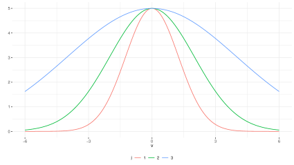
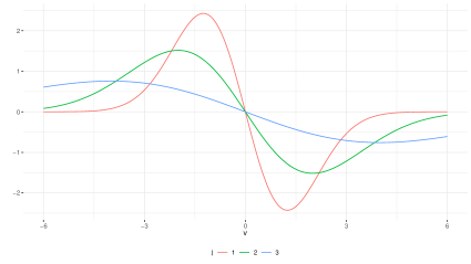
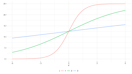
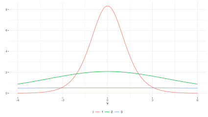
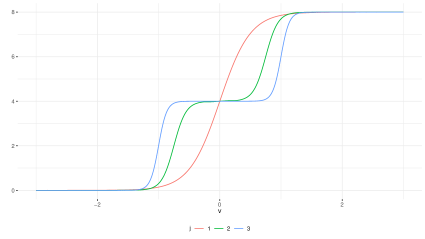
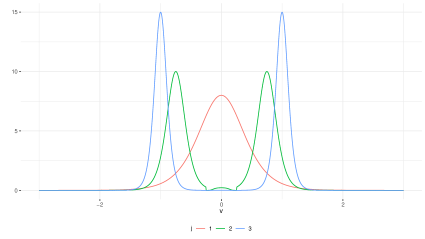
400	5.94	5.66	5.08	5.46	5.20	4.98
600	4.90	5.06	4.34	5.64	5.40	4.90
800	5.56	5.82	5.26	5.16	4.88	4.50
Wald
400	14.24	22.14	13.82	14.36	18.70	13.78
600	11.24	22.30	14.24	12.04	16.74	12.16
800	11.14	20.24	14.92	8.98	14.34	11.12

• Notes: Based on 5000 Monte carlo replications. The $Z_{k}\sim U(-1,1)$ are independently drawn.

Table S2: ERF (%) $\epsilon|\xi\sim\sqrt{5}(-1)^{\xi}\operatorname{Beta}(2,3)$, $\xi\sim\operatorname{Bernoulli}(1/2)$, $f_{j}(v)=25\left(1+\exp(-v/c_{j})\right)^{-1}$

	$X=(Z_{1},Z_{2})$			$X=(Z_{1},0.2Z_{1}+0.4Z_{2}+0.8)$
$n$	$f_{1}$	$f_{2}$	$f_{3}$	$f_{1}$	$f_{2}$	$f_{3}$
$\hat{S}$
400	4.92	5.02	4.86	6.26	5.94	5.62
600	4.56	4.40	4.74	4.90	4.96	4.90
800	4.40	4.52	4.56	4.90	4.42	4.46
Wald
400	6.94	12.62	13.06	8.12	10.86	9.72
600	5.78	10.62	15.90	6.08	8.48	9.18
800	5.70	8.64	17.84	5.56	7.92	11.08

• Notes: Based on 5000 Monte carlo replications. The $Z_{k}\sim U(-1,1)$ are independently drawn.

Table S3: ERF (%) $\epsilon=\xi/\sqrt{3/2}$, $\xi\sim t(6)$, $f_{j}(v)=5\exp(-v^{2}/2c_{j}^{2})$

	$X=(Z_{1},Z_{2})$			$X=(Z_{1},0.2Z_{1}+0.4Z_{2}+0.8)$
$n$	$f_{1}$	$f_{2}$	$f_{3}$	$f_{1}$	$f_{2}$	$f_{3}$
$\hat{S}$
400	5.18	5.14	4.56	6.04	5.86	5.64
600	5.44	5.42	5.14	5.50	5.38	5.24
800	5.32	5.62	5.12	5.10	5.14	5.58
Wald
400	14.20	23.82	13.92	15.10	19.26	13.66
600	12.50	23.52	14.74	12.20	16.62	12.92
800	10.76	19.48	16.62	10.16	15.24	12.94

• Notes: Based on 5000 Monte carlo replications. The $Z_{k}\sim U(-1,1)$ are independently drawn.

Table S4: ERF (%) $\epsilon=\xi/\sqrt{3/2}$, $\xi\sim t(6)$, $f_{j}(v)=25\left(1+\exp(-v/c_{j})\right)^{-1}$

	$X=(Z_{1},Z_{2})$			$X=(Z_{1},0.2Z_{1}+0.4Z_{2}+0.8)$
$n$	$f_{1}$	$f_{2}$	$f_{3}$	$f_{1}$	$f_{2}$	$f_{3}$
$\hat{S}$
400	5.06	5.14	5.34	6.24	5.72	5.62
600	5.44	5.38	5.38	5.70	5.54	5.62
800	5.44	4.96	4.98	5.82	5.60	5.68
Wald
400	6.94	13.02	13.18	8.26	11.18	10.22
600	6.58	10.78	15.76	7.56	8.82	9.72
800	6.54	9.28	18.20	7.20	9.14	12.48

• Notes: Based on 5000 Monte carlo replications. The $Z_{k}\sim U(-1,1)$ are independently drawn.

Table S5: ERF (%) $\epsilon\sim\mathcal{N}(0,\log(2+(X_{1}+X_{2}\theta)^{2}))$, $f_{j}(v)=5\exp(-v^{2}/2c_{j}^{2})$

	$X=(Z_{1},Z_{2})$			$X=(Z_{1},0.2Z_{1}+0.4Z_{2}+0.8)$
$n$	$f_{1}$	$f_{2}$	$f_{3}$	$f_{1}$	$f_{2}$	$f_{3}$
$\hat{S}$
400	5.84	5.70	5.30	5.36	5.26	5.12
600	5.38	5.36	5.20	5.66	5.32	4.86
800	5.52	5.50	5.50	5.74	6.06	5.70
Wald
400	18.46	30.50	14.08	19.42	23.14	15.64
600	15.12	29.20	15.06	14.90	21.86	15.46
800	13.60	24.72	17.08	14.02	21.70	14.98

• Notes: Based on 5000 Monte carlo replications. The $Z_{k}\sim U(-1,1)$ are independently drawn.

Table S6: ERF (%) $\epsilon\sim\mathcal{N}(0,\log(2+(X_{1}+X_{2}\theta)^{2}))$, $f_{j}(v)=25\left(1+\exp(-v/c_{j})\right)^{-1}$

	$X=(Z_{1},Z_{2})$			$X=(Z_{1},0.2Z_{1}+0.4Z_{2}+0.8)$
$n$	$f_{1}$	$f_{2}$	$f_{3}$	$f_{1}$	$f_{2}$	$f_{3}$
$\hat{S}$
400	5.36	5.30	5.26	6.20	5.68	5.38
600	5.40	5.34	5.42	5.50	5.54	5.52
800	5.28	5.26	5.26	5.82	5.26	5.46
Wald
400	5.88	13.52	14.90	6.64	12.94	10.84
600	4.76	10.36	20.26	5.30	10.70	11.40
800	4.30	8.82	21.86	4.56	9.64	14.28

• Notes: Based on 5000 Monte carlo replications. The $Z_{k}\sim U(-1,1)$ are independently drawn.

Table S7: ERF (%) $\epsilon\sim\mathcal{N}(0,1+\sin(X_{1})^{2})$, $f_{j}(v)=5\exp(-v^{2}/2c_{j}^{2})$

	$X=(Z_{1},Z_{2})$			$X=(Z_{1},0.2Z_{1}+0.4Z_{2}+0.8)$
$n$	$f_{1}$	$f_{2}$	$f_{3}$	$f_{1}$	$f_{2}$	$f_{3}$
$\hat{S}$
400	5.76	5.42	5.74	5.38	5.42	5.06
600	5.50	5.54	5.20	5.82	5.48	5.40
800	5.60	5.30	5.50	5.62	5.82	5.40
Wald
400	18.48	22.82	14.28	17.72	20.36	14.58
600	14.22	27.06	14.96	14.46	19.36	14.54
800	13.70	25.38	14.38	12.06	19.52	13.50

• Notes: Based on 5000 Monte carlo replications. The $Z_{k}\sim U(-1,1)$ are independently drawn.

Table S8: ERF (%) $\epsilon\sim\mathcal{N}(0,1+\sin(X_{1})^{2})$, $f_{j}(v)=25\left(1+\exp(-v/c_{j})\right)^{-1}$

	$X=(Z_{1},Z_{2})$			$X=(Z_{1},0.2Z_{1}+0.4Z_{2}+0.8)$
$n$	$f_{1}$	$f_{2}$	$f_{3}$	$f_{1}$	$f_{2}$	$f_{3}$
$\hat{S}$
400	5.28	5.10	5.18	6.06	5.68	5.24
600	5.38	5.26	5.50	5.44	5.32	5.24
800	5.02	5.10	5.04	5.66	5.42	5.46
Wald
400	8.48	14.88	12.14	8.68	13.12	10.00
600	7.90	13.10	14.10	6.80	11.60	9.90
800	7.40	11.60	16.98	6.16	9.54	11.56

• Notes: Based on 5000 Monte carlo replications. The $Z_{k}\sim U(-1,1)$ are independently drawn.

Table S9: ERF (%) $f_{j}(v)=5\exp(-v^{2}/2c_{j}^{2})$

		$X=(Z_{1},Z_{2})$					$X=(Z_{1},0.2Z_{1}+0.4Z_{2}+0.8)$
$n$	j	$10^{-1}$	$10^{-3}$	$10^{-5}$	$10^{-7}$	0	$10^{-1}$	$10^{-3}$	$10^{-5}$	$10^{-7}$	0
$\epsilon\sim\eta_{0}$
400	1	5.86	5.86	5.86	5.86	5.86	4.06	5.30	5.30	5.30	5.30
400	2	1.32	5.58	5.58	5.58	5.58	0.34	5.14	5.14	5.14	5.14
400	3	0.38	5.12	5.64	5.64	5.64	0.16	4.30	4.64	4.64	4.64
600	1	5.60	5.60	5.60	5.60	5.60	3.88	5.76	5.76	5.76	5.76
600	2	0.94	5.50	5.50	5.50	5.50	0.28	5.66	5.66	5.66	5.66
600	3	0.44	5.08	5.36	5.36	5.36	0.06	4.96	5.14	5.14	5.14
800	1	5.58	5.58	5.58	5.58	5.58	3.74	5.70	5.70	5.70	5.70
800	2	0.76	5.32	5.32	5.32	5.32	0.18	5.62	5.62	5.62	5.62
800	3	0.34	5.20	5.42	5.42	5.42	0.08	5.42	5.56	5.56	5.56
$\epsilon\sim\eta_{1}$
400	1	5.94	5.94	5.94	5.94	5.94	3.76	5.46	5.46	5.46	5.46
400	2	1.38	5.66	5.66	5.66	5.66	0.10	5.20	5.20	5.20	5.20
400	3	0.38	4.66	5.08	5.08	5.08	0.04	4.68	4.98	4.98	4.98
600	1	4.90	4.90	4.90	4.90	4.90	3.90	5.64	5.64	5.64	5.64
600	2	1.08	5.06	5.06	5.06	5.06	0.14	5.40	5.40	5.40	5.40
600	3	0.38	4.12	4.34	4.34	4.34	0.06	4.78	4.90	4.90	4.90
800	1	5.56	5.56	5.56	5.56	5.56	4.08	5.16	5.16	5.16	5.16
800	2	0.78	5.82	5.82	5.82	5.82	0.12	4.88	4.88	4.88	4.88
800	3	0.16	5.02	5.26	5.26	5.26	0.06	4.42	4.50	4.50	4.50
$\epsilon\sim\eta_{2}$
400	1	5.18	5.18	5.18	5.18	5.18	4.06	6.04	6.04	6.04	6.04
400	2	1.30	5.14	5.14	5.14	5.14	0.50	5.86	5.86	5.86	5.86
400	3	0.44	4.34	4.56	4.58	4.58	0.22	5.28	5.64	5.64	5.64
600	1	5.44	5.44	5.44	5.44	5.44	3.70	5.50	5.50	5.50	5.50
600	2	0.92	5.42	5.42	5.42	5.42	0.28	5.38	5.38	5.38	5.38
600	3	0.34	4.84	5.14	5.14	5.14	0.14	5.10	5.24	5.24	5.24
800	1	5.32	5.32	5.32	5.32	5.32	3.14	5.10	5.10	5.10	5.10
800	2	0.74	5.62	5.62	5.62	5.62	0.22	5.14	5.14	5.14	5.14
800	3	0.26	4.86	5.12	5.12	5.12	0.14	5.40	5.58	5.58	5.58
$\epsilon\sim\eta_{3}$
400	1	5.84	5.84	5.84	5.84	5.84	5.08	5.36	5.36	5.36	5.36
400	2	1.62	5.70	5.70	5.70	5.70	0.64	5.26	5.26	5.26	5.26
400	3	0.56	4.94	5.30	5.30	5.30	0.32	4.86	5.12	5.12	5.12
600	1	5.38	5.38	5.38	5.38	5.38	5.30	5.66	5.66	5.66	5.66
600	2	1.26	5.36	5.36	5.36	5.36	0.46	5.32	5.32	5.32	5.32
600	3	0.40	4.94	5.20	5.20	5.20	0.14	4.74	4.86	4.86	4.86
800	1	5.52	5.52	5.52	5.52	5.52	5.58	5.74	5.74	5.74	5.74
800	2	0.94	5.50	5.50	5.50	5.50	0.50	6.06	6.06	6.06	6.06
800	3	0.36	5.36	5.50	5.50	5.50	0.14	5.50	5.70	5.70	5.70
$\epsilon\sim\eta_{4}$
400	1	5.76	5.76	5.76	5.76	5.76	5.18	5.38	5.38	5.38	5.38
400	2	2.22	5.42	5.42	5.42	5.42	0.64	5.42	5.42	5.42	5.42
400	3	0.70	5.28	5.74	5.74	5.74	0.32	4.80	5.06	5.06	5.06
600	1	5.50	5.50	5.50	5.50	5.50	5.52	5.82	5.82	5.82	5.82
600	2	2.00	5.54	5.54	5.54	5.54	0.46	5.48	5.48	5.48	5.48
600	3	0.70	5.02	5.20	5.20	5.20	0.14	5.32	5.40	5.40	5.40
800	1	5.60	5.60	5.60	5.60	5.60	5.46	5.62	5.62	5.62	5.62
800	2	1.66	5.30	5.30	5.30	5.30	0.52	5.82	5.82	5.82	5.82
800	3	0.38	5.34	5.50	5.50	5.50	0.18	5.28	5.40	5.40	5.40

• Notes: Based on 5000 Monte carlo replications. The $Z_{k}\sim U(-1,1)$ are independently drawn.

Table S10: ERF (%) $f_{j}(v)=25\left(1+\exp(-v/c_{j})\right)^{-1}$

		$X=(Z_{1},Z_{2})$					$X=(Z_{1},0.2Z_{1}+0.4Z_{2}+0.8)$
$n$	j	$10^{-1}$	$10^{-3}$	$10^{-5}$	$10^{-7}$	0	$10^{-1}$	$10^{-3}$	$10^{-5}$	$10^{-7}$	0
$\epsilon\sim\eta_{0}$
400	1	5.32	5.32	5.32	5.32	5.32	6.02	6.02	6.02	6.02	6.02
400	2	5.16	5.16	5.16	5.16	5.16	5.38	5.52	5.52	5.52	5.52
400	3	0.50	5.16	5.16	5.16	5.16	0.22	5.32	5.32	5.32	5.32
600	1	5.32	5.32	5.32	5.32	5.32	5.62	5.62	5.62	5.62	5.62
600	2	5.44	5.44	5.44	5.44	5.44	5.32	5.36	5.36	5.36	5.36
600	3	0.28	5.34	5.34	5.34	5.34	0.06	5.26	5.26	5.26	5.26
800	1	5.12	5.12	5.12	5.12	5.12	5.66	5.66	5.66	5.66	5.66
800	2	5.26	5.26	5.26	5.26	5.26	5.40	5.42	5.42	5.42	5.42
800	3	0.32	5.20	5.20	5.20	5.20	0.08	5.40	5.40	5.40	5.40
$\epsilon\sim\eta_{1}$
400	1	4.92	4.92	4.92	4.92	4.92	6.26	6.26	6.26	6.26	6.26
400	2	5.02	5.02	5.02	5.02	5.02	5.88	5.94	5.94	5.94	5.94
400	3	0.40	4.86	4.86	4.86	4.86	0.10	5.62	5.62	5.62	5.62
600	1	4.56	4.56	4.56	4.56	4.56	4.90	4.90	4.90	4.90	4.90
600	2	4.40	4.40	4.40	4.40	4.40	4.94	4.96	4.96	4.96	4.96
600	3	0.50	4.74	4.74	4.74	4.74	0.08	4.90	4.90	4.90	4.90
800	1	4.40	4.40	4.40	4.40	4.40	4.90	4.90	4.90	4.90	4.90
800	2	4.52	4.52	4.52	4.52	4.52	4.42	4.42	4.42	4.42	4.42
800	3	0.22	4.56	4.56	4.56	4.56	0.08	4.46	4.46	4.46	4.46
$\epsilon\sim\eta_{2}$
400	1	5.06	5.06	5.06	5.06	5.06	6.24	6.24	6.24	6.24	6.24
400	2	5.14	5.14	5.14	5.14	5.14	5.56	5.72	5.72	5.72	5.72
400	3	0.66	5.34	5.34	5.34	5.34	0.20	5.62	5.62	5.62	5.62
600	1	5.44	5.44	5.44	5.44	5.44	5.70	5.70	5.70	5.70	5.70
600	2	5.38	5.38	5.38	5.38	5.38	5.32	5.54	5.54	5.54	5.54
600	3	0.46	5.38	5.38	5.38	5.38	0.14	5.62	5.62	5.62	5.62
800	1	5.44	5.44	5.44	5.44	5.44	5.82	5.82	5.82	5.82	5.82
800	2	4.96	4.96	4.96	4.96	4.96	5.56	5.60	5.60	5.60	5.60
800	3	0.26	4.98	4.98	4.98	4.98	0.16	5.68	5.68	5.68	5.68
$\epsilon\sim\eta_{3}$
400	1	5.36	5.36	5.36	5.36	5.36	6.20	6.20	6.20	6.20	6.20
400	2	5.30	5.30	5.30	5.30	5.30	5.56	5.68	5.68	5.68	5.68
400	3	0.72	5.26	5.26	5.26	5.26	0.40	5.38	5.38	5.38	5.38
600	1	5.40	5.40	5.40	5.40	5.40	5.50	5.50	5.50	5.50	5.50
600	2	5.34	5.34	5.34	5.34	5.34	5.52	5.54	5.54	5.54	5.54
600	3	0.58	5.42	5.42	5.42	5.42	0.22	5.52	5.52	5.52	5.52
800	1	5.28	5.28	5.28	5.28	5.28	5.82	5.82	5.82	5.82	5.82
800	2	5.26	5.26	5.26	5.26	5.26	5.24	5.26	5.26	5.26	5.26
800	3	0.52	5.26	5.26	5.26	5.26	0.14	5.46	5.46	5.46	5.46
$\epsilon\sim\eta_{4}$
400	1	5.28	5.28	5.28	5.28	5.28	6.06	6.06	6.06	6.06	6.06
400	2	5.10	5.10	5.10	5.10	5.10	5.68	5.68	5.68	5.68	5.68
400	3	1.22	5.18	5.18	5.18	5.18	0.32	5.24	5.24	5.24	5.24
600	1	5.38	5.38	5.38	5.38	5.38	5.44	5.44	5.44	5.44	5.44
600	2	5.26	5.26	5.26	5.26	5.26	5.32	5.32	5.32	5.32	5.32
600	3	0.88	5.50	5.50	5.50	5.50	0.16	5.24	5.24	5.24	5.24
800	1	5.02	5.02	5.02	5.02	5.02	5.66	5.66	5.66	5.66	5.66
800	2	5.10	5.10	5.10	5.10	5.10	5.42	5.42	5.42	5.42	5.42
800	3	0.76	5.04	5.04	5.04	5.04	0.22	5.46	5.46	5.46	5.46

• Notes: Based on 5000 Monte carlo replications. The $Z_{k}\sim U(-1,1)$ are independently drawn.

Table S11: ERF (%) $\epsilon|\xi\sim\sqrt{5}(-1)^{\xi}\operatorname{Beta}(2,3)$, index function as in (S35)

	$X=(Z_{1},Z_{2})$			$X=(Z_{1},0.2Z_{1}+0.4Z_{2}+0.8)$
$n$	$f_{1}$	$f_{2}$	$f_{3}$	$f_{1}$	$f_{2}$	$f_{3}$
$\hat{S}$
400	6.40	6.22	5.50	7.12	6.42	5.54
600	5.86	5.52	5.26	5.92	5.86	5.26
800	5.60	5.22	4.90	5.26	5.72	5.08
Wald
400	13.32	7.22	3.66	14.28	7.96	3.76
600	11.70	7.34	2.66	12.46	7.62	2.12
800	10.22	6.36	1.14	9.84	7.04	1.14

• Notes: Based on 5000 Monte carlo replications. The $Z_{k}\sim U(-3/2,3/2)$ are independently drawn.

Table S12: ERF (%) $\epsilon=\xi/\sqrt{3/2}$, $\xi\sim t(6)$,, index function as in (S35)

	$X=(Z_{1},Z_{2})$			$X=(Z_{1},0.2Z_{1}+0.4Z_{2}+0.8)$
$n$	$f_{1}$	$f_{2}$	$f_{3}$	$f_{1}$	$f_{2}$	$f_{3}$
$\hat{S}$
400	6.32	6.34	5.88	6.48	5.56	5.16
600	6.12	5.50	5.08	6.26	5.52	5.24
800	5.76	5.56	4.38	5.52	5.32	4.86
Wald
400	13.12	8.52	3.68	13.62	7.94	3.62
600	11.20	6.82	2.50	11.84	7.18	2.30
800	11.28	6.30	1.64	10.72	7.12	1.14

• Notes: Based on 5000 Monte carlo replications. The $Z_{k}\sim U(-3/2,3/2)$ are independently drawn.

Table S13: ERF (%) $\epsilon\sim\mathcal{N}(0,\log(2+(X_{1}+X_{2}\theta)^{2}))$, index function as in (S35)

	$X=(Z_{1},Z_{2})$			$X=(Z_{1},0.2Z_{1}+0.4Z_{2}+0.8)$
$n$	$f_{1}$	$f_{2}$	$f_{3}$	$f_{1}$	$f_{2}$	$f_{3}$
$\hat{S}$
400	6.74	6.42	6.28	6.74	6.32	5.78
600	6.32	5.60	5.74	5.56	5.94	5.42
800	5.64	5.64	4.80	6.20	5.28	5.18
Wald
400	11.36	9.58	5.74	10.96	9.22	5.64
600	9.38	7.20	2.92	8.96	7.84	3.00
800	7.46	7.04	1.80	8.78	7.10	1.76

• Notes: Based on 5000 Monte carlo replications. The $Z_{k}\sim U(-3/2,3/2)$ are independently drawn.

Table S14: ERF (%) $\epsilon\sim\mathcal{N}(0,\log(2+(X_{1}+X_{2}\theta)^{2}))$, index function as in (S35)

	$X=(Z_{1},Z_{2})$			$X=(Z_{1},0.2Z_{1}+0.4Z_{2}+0.8)$
$n$	$f_{1}$	$f_{2}$	$f_{3}$	$f_{1}$	$f_{2}$	$f_{3}$
$\hat{S}$
400	6.42	5.72	6.54	6.40	6.02	5.92
600	6.30	5.50	5.46	5.28	5.36	5.92
800	5.56	5.56	5.26	5.88	5.64	5.18
Wald
400	10.50	8.80	5.86	12.02	9.80	5.64
600	9.22	7.56	3.48	9.66	7.62	3.46
800	7.80	6.58	2.38	8.00	7.50	2.62

• Notes: Based on 5000 Monte carlo replications. The $Z_{k}\sim U(-3/2,3/2)$ are independently drawn.

Figure S7: ERF (%) $\epsilon\sim\mathcal{N}(0,1)$, index function as in (S35), $X=(Z_{1},0.2Z_{2}+0.4Z_{2}+0.8)$

Based on 5000 Monte carlo replications. The $Z_{k}\sim U(-3/2,3/2)$ are independently drawn.

Figure S8: $\pi_{j}(z)=5\exp(-z^{2}/2c_{j}^{2})$

Figure S9: $\pi_{j}(z)=25(1+\exp(-z/c_{j}))^{-1}$

Figure S10: $\pi_{j}(z)=c_{j}z$

Table S15: Empirical rejection frequencies, Design 1

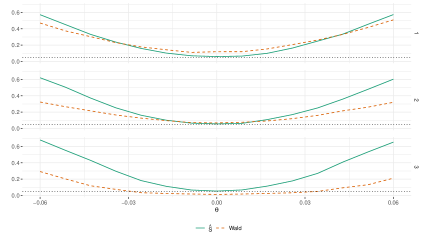
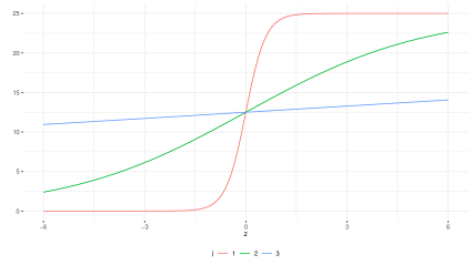
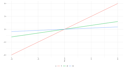
		k = 6					AIC					BIC
$n$	$j$	$10^{-1}$	$10^{-3}$	$10^{-5}$	$10^{-7}$	0	$10^{-1}$	$10^{-3}$	$10^{-5}$	$10^{-7}$	0	$10^{-1}$	$10^{-3}$	$10^{-5}$	$10^{-7}$	0
Exponential
200	1	5.78	5.78	5.78	5.78	5.78	5.78	5.78	5.78	5.78	5.78	5.70	5.70	5.70	5.70	5.70
200	2	6.16	6.16	6.16	6.16	6.16	6.16	6.16	6.16	6.16	6.16	6.20	6.20	6.20	6.20	6.20
200	3	6.14	9.32	9.32	9.32	9.32	6.14	9.32	9.32	9.32	9.32	6.38	9.00	9.00	9.00	9.00
400	1	5.18	5.18	5.18	5.18	5.18	5.18	5.18	5.18	5.18	5.18	5.08	5.08	5.08	5.08	5.08
400	2	5.74	5.74	5.74	5.74	5.74	5.74	5.74	5.74	5.74	5.74	5.60	5.60	5.60	5.60	5.60
400	3	3.18	8.70	8.70	8.70	8.70	3.18	8.70	8.70	8.70	8.70	3.72	8.40	8.40	8.40	8.40
600	1	5.30	5.30	5.30	5.30	5.30	5.30	5.30	5.30	5.30	5.30	5.30	5.30	5.30	5.30	5.30
600	2	5.50	5.50	5.50	5.50	5.50	5.50	5.50	5.50	5.50	5.50	5.40	5.40	5.40	5.40	5.40
600	3	2.14	7.92	7.92	7.92	7.92	2.14	7.92	7.92	7.92	7.92	2.64	7.86	7.86	7.86	7.86
Logistic
200	1	5.00	5.00	5.00	5.00	5.00	5.00	5.00	5.00	5.00	5.00	4.52	4.52	4.52	4.52	4.52
200	2	4.74	4.74	4.74	4.74	4.74	4.74	4.74	4.74	4.74	4.74	4.78	4.78	4.78	4.78	4.78
200	3	6.80	9.20	9.20	9.20	9.20	6.80	9.20	9.20	9.20	9.20	6.92	8.64	8.64	8.64	8.64
400	1	4.86	4.86	4.86	4.86	4.86	4.60	4.60	4.60	4.60	4.60	4.54	4.54	4.54	4.54	4.54
400	2	5.04	5.04	5.04	5.04	5.04	5.04	5.04	5.04	5.04	5.04	5.00	5.00	5.00	5.00	5.00
400	3	4.26	8.58	8.58	8.58	8.58	4.26	8.58	8.58	8.58	8.58	4.62	7.96	7.96	7.96	7.96
600	1	5.46	5.46	5.46	5.46	5.46	5.30	5.30	5.30	5.30	5.30	4.76	4.76	4.76	4.76	4.76
600	2	5.46	5.46	5.46	5.46	5.46	5.46	5.46	5.46	5.46	5.46	5.44	5.44	5.44	5.44	5.44
600	3	3.68	8.08	8.08	8.08	8.08	3.68	8.08	8.08	8.08	8.08	3.92	7.62	7.62	7.62	7.62
Linear
200	1	5.32	5.32	5.32	5.32	5.32	5.32	5.32	5.32	5.32	5.32	5.50	5.50	5.50	5.50	5.50
200	2	7.04	8.56	8.56	8.56	8.56	7.04	8.56	8.56	8.56	8.56	7.06	8.14	8.14	8.14	8.14
200	3	4.66	11.38	11.38	11.38	11.38	4.66	11.38	11.38	11.38	11.38	5.28	10.60	10.60	10.60	10.60
400	1	5.32	5.32	5.32	5.32	5.32	5.32	5.32	5.32	5.32	5.32	5.32	5.32	5.32	5.32	5.32
400	2	5.08	7.98	7.98	7.98	7.98	5.08	7.98	7.98	7.98	7.98	5.18	7.48	7.48	7.48	7.48
400	3	1.12	12.14	12.14	12.14	12.14	1.12	12.14	12.14	12.14	12.14	2.08	11.34	11.34	11.34	11.34
600	1	5.58	5.58	5.58	5.58	5.58	5.58	5.58	5.58	5.58	5.58	5.62	5.62	5.62	5.62	5.62
600	2	4.30	7.44	7.44	7.44	7.44	4.30	7.44	7.44	7.44	7.44	4.62	7.26	7.26	7.26	7.26
600	3	0.28	11.18	11.18	11.18	11.18	0.28	11.18	11.18	11.18	11.18	0.66	10.48	10.48	10.48	10.48

• Notes: Based on 5000 Monte carlo replications. All tests use Legendre polynomials to estimate $\pi$.

Table S16: Empirical rejection frequencies, IV, Design 2, $\pi_{1}$, $\pi_{2}$ same form with $j=5$ for $\pi_{2}$

		$\hat{S}$				AR	TSLS W	GMM W	GMM LM
$n$	$j$	OLS	$k=3$	AIC	BIC
Exponential
200	1	2.62	5.70	5.58	5.30	5.28	21.00	93.88	54.52
200	2	1.74	5.76	5.68	5.26	5.28	25.84	95.02	56.78
200	3	0.92	5.50	5.46	5.06	5.28	36.94	99.40	76.08
400	1	0.24	5.78	5.78	5.22	5.20	20.02	78.92	39.90
400	2	0.06	5.68	5.68	5.62	5.20	24.14	81.04	40.68
400	3	0.02	6.48	6.48	5.68	5.20	35.00	95.40	59.42
600	1	0.08	5.82	5.82	5.22	5.34	20.96	68.12	31.50
600	2	0.00	5.80	5.80	5.46	5.34	25.24	69.98	32.28
600	3	0.00	6.34	6.34	6.24	5.34	36.68	88.00	48.02
Logistic
200	1	5.78	5.54	3.98	4.02	5.28	8.88	87.08	47.96
200	2	5.68	5.62	5.66	5.36	5.28	8.48	85.84	47.24
200	3	4.56	5.16	5.14	4.84	5.28	8.72	95.36	60.26
400	1	5.92	6.02	5.56	4.96	5.20	7.38	66.74	32.40
400	2	5.78	5.92	5.92	5.68	5.20	7.24	65.46	31.32
400	3	4.52	6.16	6.16	5.80	5.20	7.42	79.14	42.14
600	1	5.92	5.40	5.00	4.14	5.34	7.04	53.42	27.08
600	2	5.84	5.26	5.26	4.98	5.34	6.88	52.02	26.38
600	3	4.12	5.94	5.94	5.62	5.34	6.94	63.94	32.82
Linear
200	1	5.08	5.34	5.30	4.96	5.28	17.48	99.54	83.06
200	2	4.24	5.18	5.16	4.92	5.28	15.28	99.74	85.92
200	3	2.38	5.74	5.78	5.34	5.28	15.28	99.98	95.46
400	1	5.04	6.10	6.10	5.98	5.20	12.72	98.56	77.96
400	2	3.74	6.30	6.30	5.96	5.20	11.96	98.86	79.30
400	3	0.34	6.92	6.92	6.20	5.20	12.16	99.96	91.84
600	1	5.14	5.24	5.24	4.94	5.34	12.22	96.84	74.44
600	2	3.72	6.24	6.24	5.74	5.34	11.42	97.12	74.04
600	3	0.00	6.04	6.04	5.58	5.34	11.34	99.78	88.42

• Notes: Based on 2500 Monte carlo replications. $k=3$ indicates that each univariate series forming the tensor series has $k=3$.

Table S17: Empirical rejection frequencies, IV, Design 2, $\pi_{2}=c_{3}Z_{2,2}$

		$\hat{S}$				AR	TSLS W	GMM W	GMM LM
$n$	$j$	OLS	$k=3$	AIC	BIC
Exponential
200	1	2.74	5.82	5.68	5.34	5.28	13.08	99.66	83.68
200	2	2.22	5.94	5.84	5.32	5.28	17.98	99.70	85.30
200	3	1.40	5.24	5.22	4.94	5.28	29.20	99.94	92.38
400	1	0.40	6.02	6.02	5.64	5.20	9.38	98.66	78.10
400	2	0.10	5.94	5.94	5.58	5.20	14.16	98.92	79.46
400	3	0.06	6.56	6.56	5.88	5.20	26.64	99.68	86.80
600	1	0.10	5.72	5.72	5.22	5.34	8.96	96.94	74.46
600	2	0.00	5.82	5.82	5.50	5.34	14.40	97.46	75.12
600	3	0.00	6.40	6.40	5.80	5.34	27.80	99.22	82.16
Logistic
200	1	5.16	5.60	4.42	4.64	5.28	18.22	99.62	82.86
200	2	5.10	5.62	5.56	5.40	5.28	17.94	99.62	83.70
200	3	4.52	5.30	5.30	5.04	5.28	14.74	99.80	86.88
400	1	5.00	6.16	5.94	5.12	5.20	13.22	98.72	78.72
400	2	5.02	6.16	6.16	5.94	5.20	13.04	98.70	79.14
400	3	4.00	6.28	6.28	5.94	5.20	11.84	99.04	80.50
600	1	5.20	5.60	4.72	4.12	5.34	12.52	97.32	74.84
600	2	5.14	5.46	5.46	5.14	5.34	12.36	97.18	75.16
600	3	3.72	6.32	6.32	5.88	5.34	11.34	97.44	74.64
Linear
200	1	5.08	5.34	5.30	4.96	5.28	17.48	99.54	83.06
200	2	4.24	5.18	5.16	4.92	5.28	15.28	99.74	85.92
200	3	2.38	5.74	5.78	5.34	5.28	15.28	99.98	95.46
400	1	5.04	6.10	6.10	5.98	5.20	12.72	98.56	77.96
400	2	3.74	6.30	6.30	5.96	5.20	11.96	98.86	79.30
400	3	0.34	6.92	6.92	6.20	5.20	12.16	99.96	91.84
600	1	5.14	5.24	5.24	4.94	5.34	12.22	96.84	74.44
600	2	3.72	6.24	6.24	5.74	5.34	11.42	97.12	74.04
600	3	0.00	6.04	6.04	5.58	5.34	11.34	99.78	88.42

• Notes: Based on 2500 Monte carlo replications. $k=3$ indicates that each univariate series forming the tensor series has $k=3$.

Table S18: Empirical rejection frequencies, IV, Design 2, $\pi_{1,j}=\pi_{2,j}$

		k = 3					AIC					BIC
$n$	$j$	$10^{-1}$	$10^{-3}$	$10^{-5}$	$10^{-7}$	0	$10^{-1}$	$10^{-3}$	$10^{-5}$	$10^{-7}$	0	$10^{-1}$	$10^{-3}$	$10^{-5}$	$10^{-7}$	0
Exponential
200	1	4.88	4.88	4.88	4.88	4.88	4.80	4.80	4.80	4.80	4.80	4.90	4.90	4.90	4.90	4.90
200	2	5.44	5.44	5.44	5.44	5.44	5.40	5.40	5.40	5.40	5.40	5.14	5.14	5.14	5.14	5.14
200	3	5.50	5.08	5.08	5.08	5.08	5.46	5.04	5.04	5.04	5.04	5.06	4.76	4.76	4.76	4.76
400	1	4.82	4.82	4.82	4.82	4.82	4.82	4.82	4.82	4.82	4.82	4.64	4.64	4.64	4.64	4.64
400	2	4.96	4.96	4.96	4.96	4.96	4.96	4.96	4.96	4.96	4.96	4.82	4.82	4.82	4.82	4.82
400	3	6.48	5.88	5.88	5.88	5.88	6.48	5.88	5.88	5.88	5.88	5.68	5.44	5.44	5.44	5.44
600	1	4.64	4.64	4.64	4.64	4.64	4.64	4.64	4.64	4.64	4.64	4.80	4.80	4.80	4.80	4.80
600	2	5.04	5.04	5.04	5.04	5.04	5.04	5.04	5.04	5.04	5.04	5.08	5.08	5.08	5.08	5.08
600	3	6.34	6.28	6.28	6.28	6.28	6.34	6.28	6.28	6.28	6.28	6.24	6.10	6.10	6.10	6.10
Logistic
200	1	4.56	4.56	4.56	4.56	4.56	1.86	1.86	1.86	1.86	1.86	2.42	2.42	2.42	2.42	2.42
200	2	4.52	4.52	4.52	4.52	4.52	4.56	4.56	4.56	4.56	4.56	4.56	4.56	4.56	4.56	4.56
200	3	5.16	4.98	4.98	4.98	4.98	5.14	4.96	4.96	4.96	4.96	4.84	4.70	4.70	4.70	4.70
400	1	5.14	5.14	5.14	5.14	5.14	3.34	3.34	3.34	3.34	3.34	3.12	3.12	3.12	3.12	3.12
400	2	4.78	4.78	4.78	4.78	4.78	4.78	4.78	4.78	4.78	4.78	4.80	4.80	4.80	4.80	4.80
400	3	6.16	5.76	5.76	5.76	5.76	6.16	5.76	5.76	5.76	5.76	5.80	5.72	5.72	5.72	5.72
600	1	4.40	4.40	4.40	4.40	4.40	3.64	3.64	3.64	3.64	3.64	3.32	3.32	3.32	3.32	3.32
600	2	4.82	4.82	4.82	4.82	4.82	4.82	4.82	4.82	4.82	4.82	4.54	4.54	4.54	4.54	4.54
600	3	5.94	5.46	5.46	5.46	5.46	5.94	5.46	5.46	5.46	5.46	5.62	5.10	5.10	5.10	5.10
Linear
200	1	4.92	4.92	4.92	4.92	4.92	4.90	4.90	4.90	4.90	4.90	4.68	4.68	4.68	4.68	4.68
200	2	5.02	4.90	4.90	4.90	4.90	4.98	4.86	4.86	4.86	4.86	4.80	4.72	4.72	4.72	4.72
200	3	5.74	5.20	5.20	5.20	5.20	5.78	5.20	5.20	5.20	5.20	5.34	5.06	5.06	5.06	5.06
400	1	5.04	5.04	5.04	5.04	5.04	5.04	5.04	5.04	5.04	5.04	4.68	4.68	4.68	4.68	4.68
400	2	5.78	5.60	5.60	5.60	5.60	5.78	5.60	5.60	5.60	5.60	5.60	5.52	5.52	5.52	5.52
400	3	6.92	6.08	6.08	6.08	6.08	6.92	6.08	6.08	6.08	6.08	6.20	5.70	5.70	5.70	5.70
600	1	4.98	4.98	4.98	4.98	4.98	4.98	4.98	4.98	4.98	4.98	4.72	4.72	4.72	4.72	4.72
600	2	5.58	5.42	5.42	5.42	5.42	5.58	5.42	5.42	5.42	5.42	5.30	5.10	5.10	5.10	5.10
600	3	6.04	6.52	6.52	6.52	6.52	6.04	6.52	6.52	6.52	6.52	5.58	5.92	5.92	5.92	5.92

• Notes: Based on 2500 Monte carlo replications. $k=3$ indicates that each univariate series forming the tensor series has $k=3$.

Table S19: Empirical rejection frequencies, IV, Design 2, $\pi_{2,j}=c_{j}Z_{2,2}$

		k = 3					AIC					BIC
$n$	$j$	$10^{-1}$	$10^{-3}$	$10^{-5}$	$10^{-7}$	0	$10^{-1}$	$10^{-3}$	$10^{-5}$	$10^{-7}$	0	$10^{-1}$	$10^{-3}$	$10^{-5}$	$10^{-7}$	0
Exponential
200	1	4.74	4.74	4.74	4.74	4.74	4.68	4.68	4.68	4.68	4.68	4.66	4.66	4.66	4.66	4.66
200	2	5.54	5.54	5.54	5.54	5.54	5.44	5.44	5.44	5.44	5.44	4.90	4.90	4.90	4.90	4.90
200	3	5.24	5.02	5.02	5.02	5.02	5.22	5.00	5.00	5.00	5.00	4.94	4.78	4.78	4.78	4.78
400	1	4.98	4.98	4.98	4.98	4.98	4.98	4.98	4.98	4.98	4.98	4.96	4.96	4.96	4.96	4.96
400	2	5.62	5.70	5.70	5.70	5.70	5.62	5.70	5.70	5.70	5.70	5.36	5.42	5.42	5.42	5.42
400	3	6.56	6.52	6.52	6.52	6.52	6.56	6.52	6.52	6.52	6.52	5.88	5.86	5.86	5.86	5.86
600	1	4.64	4.64	4.64	4.64	4.64	4.64	4.64	4.64	4.64	4.64	4.22	4.22	4.22	4.22	4.22
600	2	5.64	5.70	5.70	5.70	5.70	5.64	5.70	5.70	5.70	5.70	5.40	5.48	5.48	5.48	5.48
600	3	6.40	6.02	6.02	6.02	6.02	6.40	6.02	6.02	6.02	6.02	5.80	6.08	6.08	6.08	6.08
Logistic
200	1	4.80	4.80	4.80	4.80	4.80	3.38	3.38	3.38	3.38	3.38	3.64	3.64	3.64	3.64	3.64
200	2	5.54	5.56	5.56	5.56	5.56	5.58	5.60	5.60	5.60	5.60	5.28	5.30	5.30	5.30	5.30
200	3	5.30	5.04	5.04	5.04	5.04	5.30	5.04	5.04	5.04	5.04	5.04	4.92	4.92	4.92	4.92
400	1	5.22	5.22	5.22	5.22	5.22	4.40	4.40	4.40	4.40	4.40	4.12	4.12	4.12	4.12	4.12
400	2	5.90	6.02	6.02	6.02	6.02	5.90	6.02	6.02	6.02	6.02	5.70	5.82	5.82	5.82	5.82
400	3	6.28	6.26	6.26	6.26	6.26	6.28	6.26	6.26	6.26	6.26	5.94	6.10	6.10	6.10	6.10
600	1	4.68	4.68	4.68	4.68	4.68	4.22	4.22	4.22	4.22	4.22	3.86	3.86	3.86	3.86	3.86
600	2	5.26	5.48	5.48	5.48	5.48	5.26	5.48	5.48	5.48	5.48	4.96	5.08	5.08	5.08	5.08
600	3	6.32	5.92	5.92	5.92	5.92	6.32	5.92	5.92	5.92	5.92	5.88	5.42	5.42	5.42	5.42
Linear
200	1	4.92	4.92	4.92	4.92	4.92	4.90	4.90	4.90	4.90	4.90	4.68	4.68	4.68	4.68	4.68
200	2	5.02	4.90	4.90	4.90	4.90	4.98	4.86	4.86	4.86	4.86	4.80	4.72	4.72	4.72	4.72
200	3	5.74	5.20	5.20	5.20	5.20	5.78	5.20	5.20	5.20	5.20	5.34	5.06	5.06	5.06	5.06
400	1	5.04	5.04	5.04	5.04	5.04	5.04	5.04	5.04	5.04	5.04	4.68	4.68	4.68	4.68	4.68
400	2	5.78	5.60	5.60	5.60	5.60	5.78	5.60	5.60	5.60	5.60	5.60	5.52	5.52	5.52	5.52
400	3	6.92	6.08	6.08	6.08	6.08	6.92	6.08	6.08	6.08	6.08	6.20	5.70	5.70	5.70	5.70
600	1	4.98	4.98	4.98	4.98	4.98	4.98	4.98	4.98	4.98	4.98	4.72	4.72	4.72	4.72	4.72
600	2	5.58	5.42	5.42	5.42	5.42	5.58	5.42	5.42	5.42	5.42	5.30	5.10	5.10	5.10	5.10
600	3	6.04	6.52	6.52	6.52	6.52	6.04	6.52	6.52	6.52	6.52	5.58	5.92	5.92	5.92	5.92

• Notes: Based on 2500 Monte carlo replications. $k=3$ indicates that each univariate series forming the tensor series has $k=3$.

Table S20: Empirical rejection frequencies, IV, Design 2, $\pi_{1}$, $\pi_{2}$ same form with $j=3$ for $\pi_{2}$

		k = 3					AIC					BIC
$n$	$j$	$10^{-1}$	$10^{-3}$	$10^{-5}$	$10^{-7}$	0	$10^{-1}$	$10^{-3}$	$10^{-5}$	$10^{-7}$	0	$10^{-1}$	$10^{-3}$	$10^{-5}$	$10^{-7}$	0
Exponential
200	1	5.70	5.70	5.70	5.70	5.70	5.58	5.58	5.58	5.58	5.58	5.30	5.30	5.30	5.30	5.30
200	2	5.76	5.74	5.74	5.74	5.74	5.68	5.66	5.66	5.66	5.66	5.26	5.24	5.24	5.24	5.24
200	3	5.50	5.08	5.08	5.08	5.08	5.46	5.04	5.04	5.04	5.04	5.06	4.76	4.76	4.76	4.76
400	1	5.78	5.88	5.88	5.88	5.88	5.78	5.88	5.88	5.88	5.88	5.22	5.36	5.36	5.36	5.36
400	2	5.68	5.78	5.78	5.78	5.78	5.68	5.78	5.78	5.78	5.78	5.62	5.66	5.66	5.66	5.66
400	3	6.48	5.88	5.88	5.88	5.88	6.48	5.88	5.88	5.88	5.88	5.68	5.44	5.44	5.44	5.44
600	1	5.82	5.90	5.90	5.90	5.90	5.82	5.90	5.90	5.90	5.90	5.22	5.24	5.24	5.24	5.24
600	2	5.80	6.10	6.10	6.10	6.10	5.80	6.10	6.10	6.10	6.10	5.46	5.70	5.70	5.70	5.70
600	3	6.34	6.28	6.28	6.28	6.28	6.34	6.28	6.28	6.28	6.28	6.24	6.10	6.10	6.10	6.10
Logistic
200	1	5.54	5.54	5.54	5.54	5.54	3.98	4.00	4.00	4.00	4.00	4.02	4.04	4.04	4.04	4.04
200	2	5.62	5.64	5.64	5.64	5.64	5.66	5.68	5.68	5.68	5.68	5.36	5.38	5.38	5.38	5.38
200	3	5.16	4.98	4.98	4.98	4.98	5.14	4.96	4.96	4.96	4.96	4.84	4.70	4.70	4.70	4.70
400	1	6.02	6.12	6.12	6.12	6.12	5.56	5.62	5.62	5.62	5.62	4.96	5.10	5.10	5.10	5.10
400	2	5.92	6.10	6.10	6.10	6.10	5.92	6.10	6.10	6.10	6.10	5.68	5.88	5.88	5.88	5.88
400	3	6.16	5.76	5.76	5.76	5.76	6.16	5.76	5.76	5.76	5.76	5.80	5.72	5.72	5.72	5.72
600	1	5.40	5.64	5.64	5.64	5.64	5.00	5.16	5.16	5.16	5.16	4.14	4.36	4.36	4.36	4.36
600	2	5.26	5.64	5.64	5.64	5.64	5.26	5.64	5.64	5.64	5.64	4.98	5.20	5.20	5.20	5.20
600	3	5.94	5.46	5.46	5.46	5.46	5.94	5.46	5.46	5.46	5.46	5.62	5.10	5.10	5.10	5.10
Linear
200	1	5.34	5.30	5.30	5.30	5.30	5.30	5.28	5.28	5.28	5.28	4.96	4.96	4.96	4.96	4.96
200	2	5.18	4.96	4.96	4.96	4.96	5.16	4.94	4.94	4.94	4.94	4.92	4.90	4.90	4.90	4.90
200	3	5.74	5.20	5.20	5.20	5.20	5.78	5.20	5.20	5.20	5.20	5.34	5.06	5.06	5.06	5.06
400	1	6.10	6.26	6.26	6.26	6.26	6.10	6.26	6.26	6.26	6.26	5.98	6.10	6.10	6.10	6.10
400	2	6.30	6.34	6.34	6.34	6.34	6.30	6.34	6.34	6.34	6.34	5.96	6.18	6.18	6.18	6.18
400	3	6.92	6.08	6.08	6.08	6.08	6.92	6.08	6.08	6.08	6.08	6.20	5.70	5.70	5.70	5.70
600	1	5.24	6.14	6.14	6.14	6.14	5.24	6.14	6.14	6.14	6.14	4.94	5.58	5.58	5.58	5.58
600	2	6.24	5.98	5.98	5.98	5.98	6.24	5.98	5.98	5.98	5.98	5.74	5.42	5.42	5.42	5.42
600	3	6.04	6.52	6.52	6.52	6.52	6.04	6.52	6.52	6.52	6.52	5.58	5.92	5.92	5.92	5.92

• Notes: Based on 2500 Monte carlo replications. $k=3$ indicates that each univariate series forming the tensor series has $k=3$.

Table S21: Empirical rejection frequencies, IV, Design 2, $\pi_{2}=c_{5}Z_{2,2}$

		k = 3					AIC					BIC
$n$	$j$	$10^{-1}$	$10^{-3}$	$10^{-5}$	$10^{-7}$	0	$10^{-1}$	$10^{-3}$	$10^{-5}$	$10^{-7}$	0	$10^{-1}$	$10^{-3}$	$10^{-5}$	$10^{-7}$	0
Exponential
200	1	5.82	5.80	5.80	5.80	5.80	5.68	5.66	5.66	5.66	5.66	5.34	5.34	5.34	5.34	5.34
200	2	5.94	5.92	5.92	5.92	5.92	5.84	5.82	5.82	5.82	5.82	5.32	5.28	5.28	5.28	5.28
200	3	5.24	5.02	5.02	5.02	5.02	5.22	5.00	5.00	5.00	5.00	4.94	4.78	4.78	4.78	4.78
400	1	6.02	6.38	6.38	6.38	6.38	6.02	6.38	6.38	6.38	6.38	5.64	5.80	5.80	5.80	5.80
400	2	5.94	6.26	6.26	6.26	6.26	5.94	6.26	6.26	6.26	6.26	5.58	5.94	5.94	5.94	5.94
400	3	6.56	6.52	6.52	6.52	6.52	6.56	6.52	6.52	6.52	6.52	5.88	5.86	5.86	5.86	5.86
600	1	5.72	6.68	6.68	6.68	6.68	5.72	6.68	6.68	6.68	6.68	5.22	5.82	5.82	5.82	5.82
600	2	5.82	6.74	6.74	6.74	6.74	5.82	6.74	6.74	6.74	6.74	5.50	6.00	6.00	6.00	6.00
600	3	6.40	6.02	6.02	6.02	6.02	6.40	6.02	6.02	6.02	6.02	5.80	6.08	6.08	6.08	6.08
Logistic
200	1	5.60	5.58	5.58	5.58	5.58	4.42	4.44	4.44	4.44	4.44	4.64	4.64	4.64	4.64	4.64
200	2	5.62	5.58	5.58	5.58	5.58	5.56	5.54	5.54	5.54	5.54	5.40	5.36	5.36	5.36	5.36
200	3	5.30	5.04	5.04	5.04	5.04	5.30	5.04	5.04	5.04	5.04	5.04	4.92	4.92	4.92	4.92
400	1	6.16	6.48	6.48	6.48	6.48	5.94	6.26	6.26	6.26	6.26	5.12	5.44	5.44	5.44	5.44
400	2	6.16	6.30	6.30	6.30	6.30	6.16	6.30	6.30	6.30	6.30	5.94	6.06	6.06	6.06	6.06
400	3	6.28	6.26	6.26	6.26	6.26	6.28	6.26	6.26	6.26	6.26	5.94	6.10	6.10	6.10	6.10
600	1	5.60	6.26	6.26	6.26	6.26	4.72	5.72	5.72	5.72	5.72	4.12	4.92	4.92	4.92	4.92
600	2	5.46	6.16	6.16	6.16	6.16	5.46	6.16	6.16	6.16	6.16	5.14	5.66	5.66	5.66	5.66
600	3	6.32	5.92	5.92	5.92	5.92	6.32	5.92	5.92	5.92	5.92	5.88	5.42	5.42	5.42	5.42
Linear
200	1	5.34	5.30	5.30	5.30	5.30	5.30	5.28	5.28	5.28	5.28	4.96	4.96	4.96	4.96	4.96
200	2	5.18	4.96	4.96	4.96	4.96	5.16	4.94	4.94	4.94	4.94	4.92	4.90	4.90	4.90	4.90
200	3	5.74	5.20	5.20	5.20	5.20	5.78	5.20	5.20	5.20	5.20	5.34	5.06	5.06	5.06	5.06
400	1	6.10	6.26	6.26	6.26	6.26	6.10	6.26	6.26	6.26	6.26	5.98	6.10	6.10	6.10	6.10
400	2	6.30	6.34	6.34	6.34	6.34	6.30	6.34	6.34	6.34	6.34	5.96	6.18	6.18	6.18	6.18
400	3	6.92	6.08	6.08	6.08	6.08	6.92	6.08	6.08	6.08	6.08	6.20	5.70	5.70	5.70	5.70
600	1	5.24	6.14	6.14	6.14	6.14	5.24	6.14	6.14	6.14	6.14	4.94	5.58	5.58	5.58	5.58
600	2	6.24	5.98	5.98	5.98	5.98	6.24	5.98	5.98	5.98	5.98	5.74	5.42	5.42	5.42	5.42
600	3	6.04	6.52	6.52	6.52	6.52	6.04	6.52	6.52	6.52	6.52	5.58	5.92	5.92	5.92	5.92

• Notes: Based on 2500 Monte carlo replications. $k=3$ indicates that each univariate series forming the tensor series has $k=3$.

Figure S11: $\pi_{i}$ exponential with $j=1$ $(i=1,2)$

(a) $\hat{S}$ (AIC)

(b) $\hat{S}$ (BIC)

Figure S12: $\pi_{1}$ exponential with $j=1$, $\pi_{2}$ exponential with $j=3$

(a) $\hat{S}$ (AIC)

(b) $\hat{S}$ (BIC)

Figure S13: $\pi_{1}$ exponential with $j=3$, $\pi_{2}$ exponential with $j=3$

(a) $\hat{S}$ (AIC)

(b) $\hat{S}$ (BIC)

Figure S14: $\pi_{i}$ logistic with $j=1$ $(i=1,2)$

(a) $\hat{S}$ (AIC)

(b) $\hat{S}$ (BIC)

Figure S15: $\pi_{1}$ logistic with $j=1$, $\pi_{2}$ logistic with $j=3$

(a) $\hat{S}$ (AIC)

(b) $\hat{S}$ (BIC)

Figure S16: $\pi_{1}$ logistic with $j=3$, $\pi_{2}$ logistic with $j=3$

(a) $\hat{S}$ (AIC)

(b) $\hat{S}$ (BIC)

Figure S17: $\pi_{i}$ linear with $j=1$ $(i=1,2)$

(a) $\hat{S}$ (AIC)

(b) $\hat{S}$ (BIC)

Figure S18: $\pi_{1}$ linear with $j=1$, $\pi_{2}$ linear with $j=3$

(a) $\hat{S}$ (AIC)

(b) $\hat{S}$ (BIC)

Figure S19: $\pi_{1}$ linear with $j=3$, $\pi_{2}$ linear with $j=3$

(a) $\hat{S}$ (AIC)

(b) $\hat{S}$ (BIC)

Figure S20: $\pi_{1}$ exponential with $j=1$, $\pi_{2}$ linear with $j=1$

(a) AR

(b) $\hat{S}$ ($k=3$)

Figure S21: $\pi_{1}$ exponential with $j=1$, $\pi_{2}$ linear with $j=3$

(a) AR

(b) $\hat{S}$ ($k=3$)

Figure S22: $\pi_{1}$ exponential with $j=3$, $\pi_{2}$ linear with $j=3$

(a) AR

(b) $\hat{S}$ ($k=3$)

Figure S23: $\pi_{1}$ logistic with $j=1$, $\pi_{2}$ linear with $j=1$

(a) AR

(b) $\hat{S}$ ($k=3$)

Figure S24: $\pi_{1}$ logistic with $j=1$, $\pi_{2}$ linear with $j=3$

(a) AR

(b) $\hat{S}$ ($k=3$)

Figure S25: $\pi_{1}$ logistic with $j=3$, $\pi_{2}$ linear with $j=3$

(a) AR

(b) $\hat{S}$ ($k=3$)

Table S22: Empirical rejection frequencies, Design 3

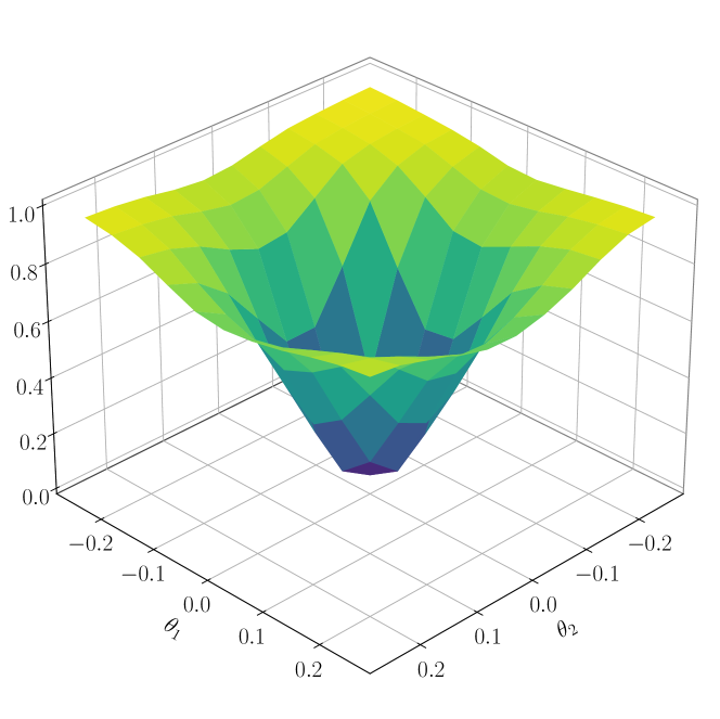
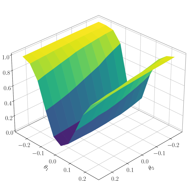
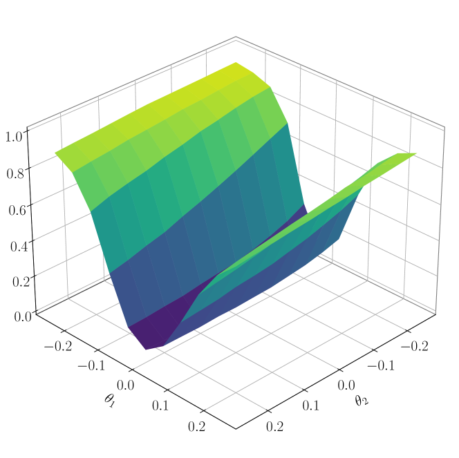
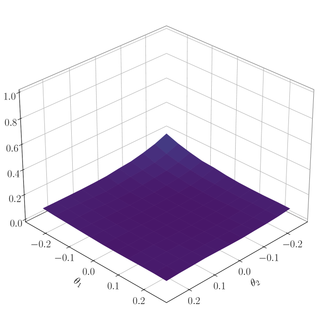
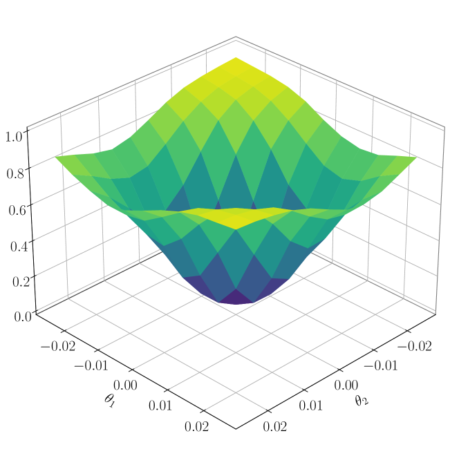
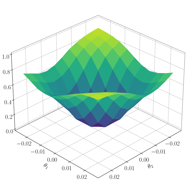
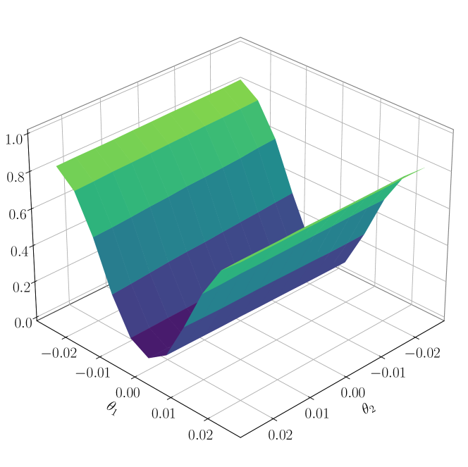
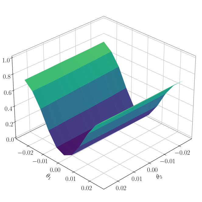
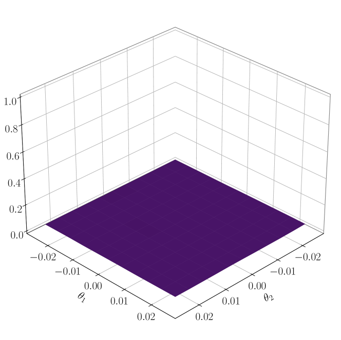
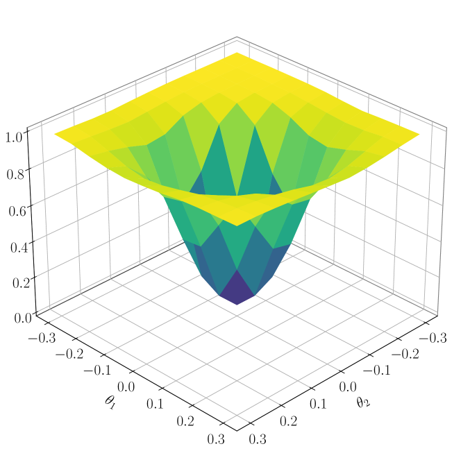
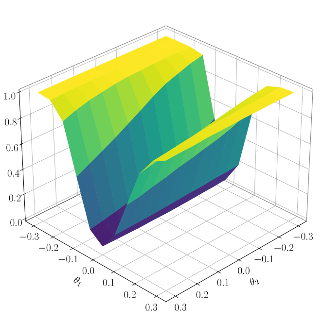
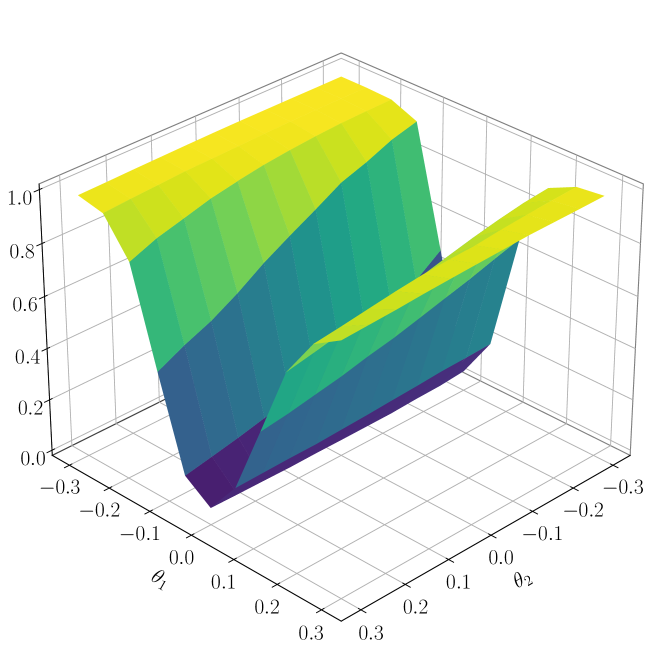
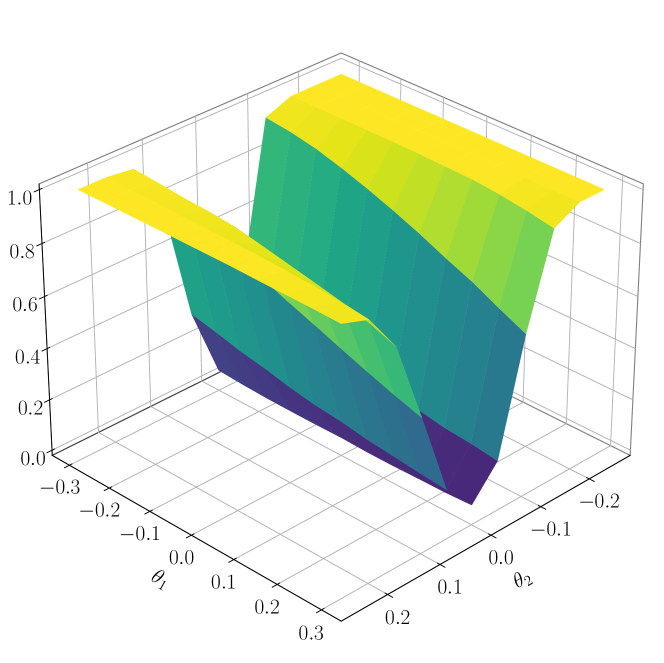
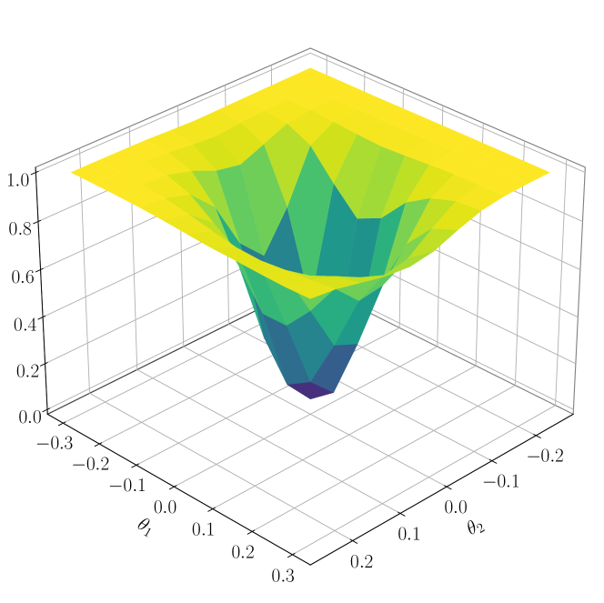
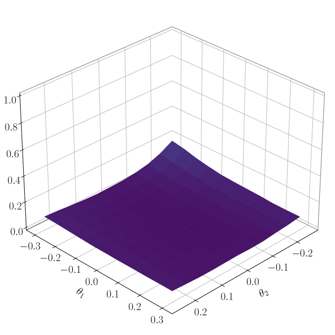
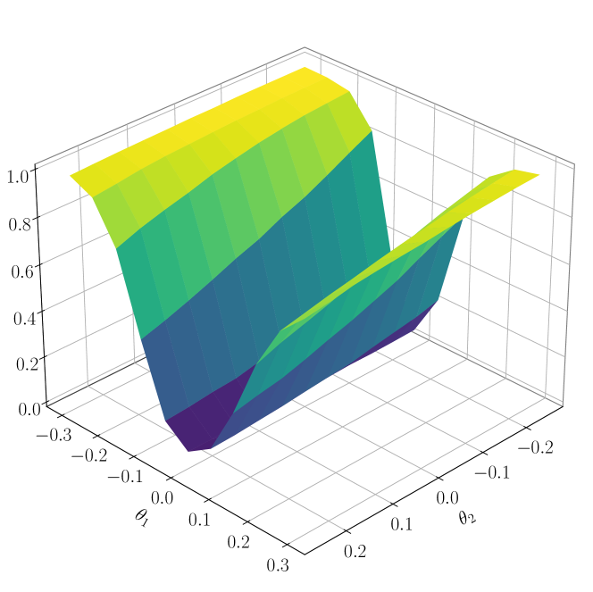
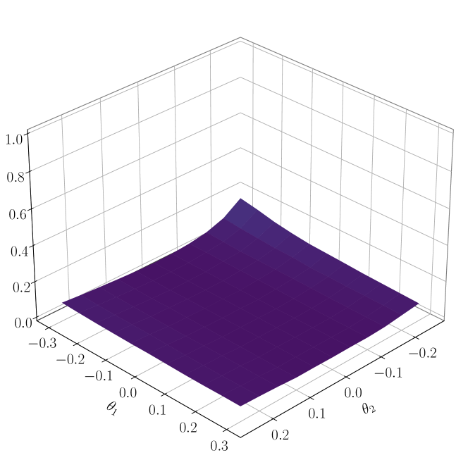
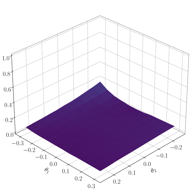
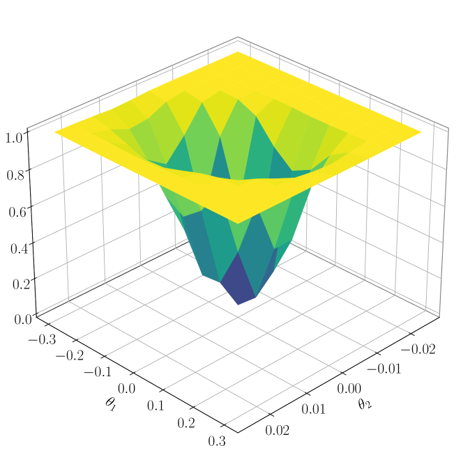
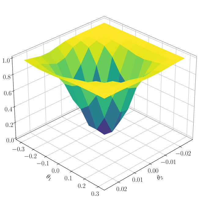
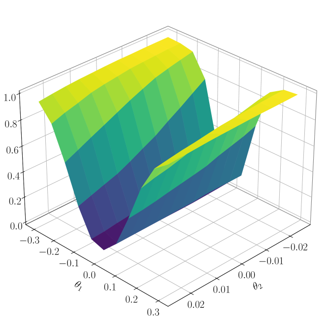
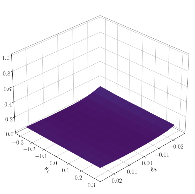
		$\hat{S}$				AR	TSLS W	GMM W	GMM LM
$n$	$j$	OLS	$k=6$	AIC	BIC
Exponential
200	1	0.78	5.64	5.64	5.60	5.54	1.24	20.10	5.22
200	2	0.28	6.28	6.28	6.22	5.54	4.62	31.56	6.10
200	3	0.04	6.30	6.30	6.32	5.54	23.32	71.74	22.60
400	1	0.06	5.12	5.12	5.06	5.46	1.48	13.74	5.20
400	2	0.02	5.52	5.52	5.62	5.46	4.32	20.96	5.50
400	3	0.00	2.68	2.68	3.20	5.46	22.78	53.20	14.82
600	1	0.02	5.14	5.14	5.08	5.78	1.44	10.98	5.34
600	2	0.00	5.80	5.80	5.84	5.78	4.78	16.76	5.60
600	3	0.00	1.42	1.42	1.94	5.78	22.50	43.78	12.54
Logistic
200	1	4.78	5.00	4.84	4.82	5.54	5.36	9.10	4.64
200	2	4.78	4.84	4.84	4.76	5.54	5.16	16.50	5.04
200	3	2.22	6.88	6.88	6.86	5.54	8.36	59.20	19.24
400	1	5.24	5.06	4.94	4.62	5.46	5.52	6.56	4.48
400	2	5.24	4.88	4.88	4.88	5.46	5.50	11.38	5.08
400	3	2.02	3.84	3.84	4.26	5.46	6.48	40.42	13.50
600	1	5.52	5.42	5.28	4.92	5.78	5.76	6.56	5.40
600	2	5.52	5.30	5.30	5.30	5.78	5.70	10.12	5.62
600	3	2.10	3.16	3.16	3.46	5.78	6.76	31.58	11.78
Linear
200	1	4.78	5.50	5.50	5.50	5.54	4.98	21.00	5.96
200	2	2.28	7.04	7.04	7.04	5.54	7.62	52.44	15.88
200	3	0.16	5.30	5.30	5.66	5.54	16.36	93.76	48.02
400	1	5.24	5.26	5.26	5.24	5.46	5.28	14.04	5.48
400	2	2.24	4.70	4.70	4.92	5.46	6.02	35.14	11.64
400	3	0.02	1.28	1.28	2.12	5.46	11.96	88.48	41.48
600	1	5.52	5.70	5.70	5.74	5.78	5.86	12.52	6.06
600	2	2.94	3.98	3.98	4.40	5.78	6.34	27.20	10.52
600	3	0.00	0.40	0.40	0.84	5.78	11.32	83.64	37.48

• Notes: Based on 5000 Monte carlo replications.

Table S23: Empirical rejection frequencies, Design 3

		k = 6					AIC					BIC
$n$	$j$	$10^{-1}$	$10^{-3}$	$10^{-5}$	$10^{-7}$	0	$10^{-1}$	$10^{-3}$	$10^{-5}$	$10^{-7}$	0	$10^{-1}$	$10^{-3}$	$10^{-5}$	$10^{-7}$	0
Exponential
200	1	5.64	5.64	5.64	5.64	5.64	5.64	5.64	5.64	5.64	5.64	5.60	5.60	5.60	5.60	5.60
200	2	6.28	6.30	6.30	6.30	6.30	6.28	6.30	6.30	6.30	6.30	6.22	6.24	6.24	6.24	6.24
200	3	6.30	9.68	9.68	9.68	9.68	6.30	9.68	9.68	9.68	9.68	6.32	9.34	9.34	9.34	9.34
400	1	5.12	5.12	5.12	5.12	5.12	5.12	5.12	5.12	5.12	5.12	5.06	5.06	5.06	5.06	5.06
400	2	5.52	5.52	5.52	5.52	5.52	5.52	5.52	5.52	5.52	5.52	5.62	5.62	5.62	5.62	5.62
400	3	2.68	9.34	9.34	9.34	9.34	2.68	9.34	9.34	9.34	9.34	3.20	9.16	9.16	9.16	9.16
600	1	5.14	5.14	5.14	5.14	5.14	5.14	5.14	5.14	5.14	5.14	5.08	5.08	5.08	5.08	5.08
600	2	5.80	5.80	5.80	5.80	5.80	5.80	5.80	5.80	5.80	5.80	5.84	5.84	5.84	5.84	5.84
600	3	1.42	8.54	8.54	8.54	8.54	1.42	8.54	8.54	8.54	8.54	1.94	8.42	8.42	8.42	8.42
Logistic
200	1	5.00	5.00	5.00	5.00	5.00	4.84	4.84	4.84	4.84	4.84	4.82	4.82	4.82	4.82	4.82
200	2	4.84	4.84	4.84	4.84	4.84	4.84	4.84	4.84	4.84	4.84	4.76	4.76	4.76	4.76	4.76
200	3	6.88	9.58	9.58	9.58	9.58	6.88	9.58	9.58	9.58	9.58	6.86	9.06	9.06	9.06	9.06
400	1	5.06	5.06	5.06	5.06	5.06	4.94	4.94	4.94	4.94	4.94	4.62	4.62	4.62	4.62	4.62
400	2	4.88	4.88	4.88	4.88	4.88	4.88	4.88	4.88	4.88	4.88	4.88	4.88	4.88	4.88	4.88
400	3	3.84	8.94	8.94	8.94	8.94	3.84	8.94	8.94	8.94	8.94	4.26	8.60	8.60	8.60	8.60
600	1	5.42	5.42	5.42	5.42	5.42	5.28	5.28	5.28	5.28	5.28	4.92	4.92	4.92	4.92	4.92
600	2	5.30	5.30	5.30	5.30	5.30	5.30	5.30	5.30	5.30	5.30	5.30	5.30	5.30	5.30	5.30
600	3	3.16	8.54	8.54	8.54	8.54	3.16	8.54	8.54	8.54	8.54	3.46	8.22	8.22	8.22	8.22
Linear
200	1	5.50	5.50	5.50	5.50	5.50	5.50	5.50	5.50	5.50	5.50	5.50	5.50	5.50	5.50	5.50
200	2	7.04	9.00	9.00	9.00	9.00	7.04	9.00	9.00	9.00	9.00	7.04	8.56	8.56	8.56	8.56
200	3	5.30	11.34	11.34	11.34	11.34	5.30	11.34	11.34	11.34	11.34	5.66	10.76	10.76	10.76	10.76
400	1	5.26	5.26	5.26	5.26	5.26	5.26	5.26	5.26	5.26	5.26	5.24	5.24	5.24	5.24	5.24
400	2	4.70	8.42	8.42	8.42	8.42	4.70	8.42	8.42	8.42	8.42	4.92	8.10	8.10	8.10	8.10
400	3	1.28	12.10	12.10	12.10	12.10	1.28	12.10	12.10	12.10	12.10	2.12	11.48	11.48	11.48	11.48
600	1	5.70	5.70	5.70	5.70	5.70	5.70	5.70	5.70	5.70	5.70	5.74	5.74	5.74	5.74	5.74
600	2	3.98	7.84	7.84	7.84	7.84	3.98	7.84	7.84	7.84	7.84	4.40	7.72	7.72	7.72	7.72
600	3	0.40	10.90	10.90	10.90	10.90	0.40	10.90	10.90	10.90	10.90	0.84	10.38	10.38	10.38	10.38

• Notes: Based on 5000 Monte carlo replications.

Figure S26: Design 3, $\pi_{j}(z)=5\exp(-z^{2}/2c_{j}^{2})$

Figure S27: Design 3, $\pi_{j}(z)=25(1+\exp(-z/c_{j}))^{-1}$

Figure S28: Design 3, $\pi_{j}(z)=c_{j}z$

Table S24: Empirical rejection frequencies, IV, Design 4, $\pi_{1}=\pi_{2}$

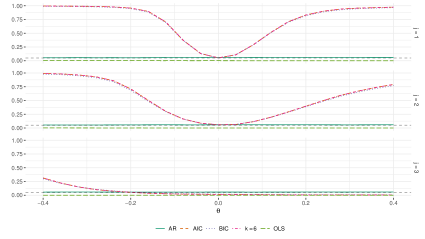
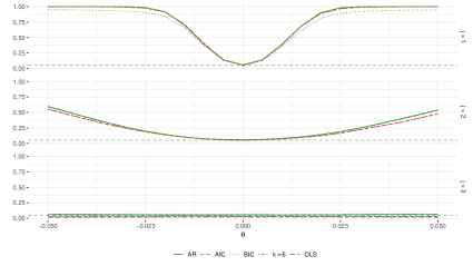
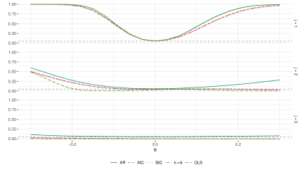
		$\hat{S}$				AR	LM	CLR	TSLS W	GMM W	GMM LM
$n$	$j$	OLS	$k=3$	AIC	BIC
Exponential
200	1	1.02	4.80	4.80	4.48	4.84	4.98	5.06	18.12	26.14	12.80
200	2	0.30	5.98	5.96	5.56	4.84	5.18	5.02	35.52	59.94	27.04
200	3	0.04	6.38	6.32	6.00	4.84	5.12	5.00	60.74	99.80	85.28
400	1	0.02	5.42	5.42	5.12	5.38	5.12	5.54	17.70	14.98	9.20
400	2	0.00	6.00	6.00	6.04	5.38	5.24	5.52	35.98	35.12	17.64
400	3	0.00	7.22	7.22	6.94	5.38	5.30	5.54	61.34	97.02	75.28
600	1	0.00	4.82	4.82	4.70	5.04	5.26	5.36	17.48	11.92	8.46
600	2	0.00	5.50	5.50	5.46	5.04	5.54	5.26	35.34	25.74	14.42
600	3	0.00	5.70	5.70	5.44	5.04	5.54	5.32	61.38	92.20	67.24
Logistic
200	1	5.40	4.60	1.32	2.78	4.84	5.40	6.86	5.44	6.10	5.72
200	2	5.42	5.32	5.26	5.00	4.84	5.36	6.72	5.62	9.64	7.14
200	3	3.58	6.32	6.26	5.62	4.84	5.48	6.60	13.60	97.44	77.14
400	1	5.12	5.22	4.28	2.70	5.38	5.30	6.52	5.18	5.52	5.36
400	2	4.88	5.48	5.48	5.14	5.38	5.34	6.60	5.04	7.20	5.80
400	3	1.92	7.38	7.38	6.86	5.38	5.16	6.24	9.82	86.10	60.82
600	1	5.10	4.58	4.36	2.28	5.04	5.36	6.50	5.28	5.36	5.50
600	2	5.06	4.98	4.98	4.94	5.04	5.38	6.54	5.22	6.70	5.72
600	3	1.16	6.22	6.22	5.80	5.04	5.38	6.36	8.58	74.12	49.12
Linear
200	1	5.32	5.68	5.62	5.10	4.84	5.44	6.74	5.86	25.98	14.34
200	2	3.80	6.26	6.20	5.62	4.84	5.42	6.72	11.74	94.78	69.16
200	3	0.14	6.22	6.10	5.66	4.84	5.26	5.92	42.12	100.00	97.30
400	1	4.74	5.92	5.92	5.32	5.38	5.32	6.48	5.48	15.60	9.72
400	2	2.94	7.18	7.18	6.72	5.38	5.22	6.30	8.92	78.00	51.38
400	3	0.00	7.40	7.40	6.78	5.38	5.04	5.72	30.70	99.88	95.96
600	1	5.02	5.32	5.32	5.26	5.04	5.40	6.56	5.46	12.44	8.62
600	2	2.64	6.44	6.44	5.98	5.04	5.42	6.38	7.92	63.18	40.16
600	3	0.00	4.52	4.52	4.32	5.04	5.26	6.02	25.00	99.52	94.34

• Notes: Based on 5000 Monte carlo replications.

Table S25: Empirical rejection frequencies, IV, Design 4, $\pi_{1}=\pi_{2}$, $\hat{S}$ tests

		k = 3					AIC					BIC
$n$	$j$	$10^{-1}$	$10^{-3}$	$10^{-5}$	$10^{-7}$	0	$10^{-1}$	$10^{-3}$	$10^{-5}$	$10^{-7}$	0	$10^{-1}$	$10^{-3}$	$10^{-5}$	$10^{-7}$	0
Exponential
200	1	4.80	4.80	4.80	4.80	4.80	4.80	4.80	4.80	4.80	4.80	4.48	4.48	4.48	4.48	4.48
200	2	5.98	5.98	5.98	5.98	5.98	5.96	5.96	5.96	5.96	5.96	5.56	5.56	5.56	5.56	5.56
200	3	6.38	6.38	6.38	6.38	6.38	6.32	6.32	6.32	6.32	6.32	6.00	6.00	6.00	6.00	6.00
400	1	5.42	5.42	5.42	5.42	5.42	5.42	5.42	5.42	5.42	5.42	5.12	5.12	5.12	5.12	5.12
400	2	6.00	6.00	6.00	6.00	6.00	6.00	6.00	6.00	6.00	6.00	6.04	6.04	6.04	6.04	6.04
400	3	7.22	7.92	7.92	7.92	7.92	7.22	7.92	7.92	7.92	7.92	6.94	7.50	7.50	7.50	7.50
600	1	4.82	4.82	4.82	4.82	4.82	4.82	4.82	4.82	4.82	4.82	4.70	4.70	4.70	4.70	4.70
600	2	5.50	5.50	5.50	5.50	5.50	5.50	5.50	5.50	5.50	5.50	5.46	5.46	5.46	5.46	5.46
600	3	5.70	7.72	7.72	7.72	7.72	5.70	7.72	7.72	7.72	7.72	5.44	7.08	7.08	7.08	7.08
Logistic
200	1	4.60	4.60	4.60	4.60	4.60	1.32	1.32	1.32	1.32	1.32	2.78	2.78	2.78	2.78	2.78
200	2	5.32	5.32	5.32	5.32	5.32	5.26	5.26	5.26	5.26	5.26	5.00	5.00	5.00	5.00	5.00
200	3	6.32	6.34	6.34	6.34	6.34	6.26	6.28	6.28	6.28	6.28	5.62	5.64	5.64	5.64	5.64
400	1	5.22	5.22	5.22	5.22	5.22	4.28	4.28	4.28	4.28	4.28	2.70	2.70	2.70	2.70	2.70
400	2	5.48	5.48	5.48	5.48	5.48	5.48	5.48	5.48	5.48	5.48	5.14	5.14	5.14	5.14	5.14
400	3	7.38	7.54	7.54	7.54	7.54	7.38	7.54	7.54	7.54	7.54	6.86	7.02	7.02	7.02	7.02
600	1	4.58	4.58	4.58	4.58	4.58	4.36	4.36	4.36	4.36	4.36	2.28	2.28	2.28	2.28	2.28
600	2	4.98	4.98	4.98	4.98	4.98	4.98	4.98	4.98	4.98	4.98	4.94	4.94	4.94	4.94	4.94
600	3	6.22	7.24	7.24	7.24	7.24	6.22	7.24	7.24	7.24	7.24	5.80	6.72	6.72	6.72	6.72
Linear
200	1	5.68	5.68	5.68	5.68	5.68	5.62	5.62	5.62	5.62	5.62	5.10	5.10	5.10	5.10	5.10
200	2	6.26	6.28	6.28	6.28	6.28	6.20	6.22	6.22	6.22	6.22	5.62	5.64	5.64	5.64	5.64
200	3	6.22	6.22	6.22	6.22	6.22	6.10	6.10	6.10	6.10	6.10	5.66	5.66	5.66	5.66	5.66
400	1	5.92	5.92	5.92	5.92	5.92	5.92	5.92	5.92	5.92	5.92	5.32	5.32	5.32	5.32	5.32
400	2	7.18	7.30	7.30	7.30	7.30	7.18	7.30	7.30	7.30	7.30	6.72	6.84	6.84	6.84	6.84
400	3	7.40	8.30	8.30	8.30	8.30	7.40	8.30	8.30	8.30	8.30	6.78	7.60	7.60	7.60	7.60
600	1	5.32	5.32	5.32	5.32	5.32	5.32	5.32	5.32	5.32	5.32	5.26	5.26	5.26	5.26	5.26
600	2	6.44	7.20	7.20	7.20	7.20	6.44	7.20	7.20	7.20	7.20	5.98	6.64	6.64	6.64	6.64
600	3	4.52	7.56	7.56	7.56	7.56	4.52	7.56	7.56	7.56	7.56	4.32	6.84	6.84	6.84	6.84

• Notes: Based on 5000 Monte carlo replications.

Figure S29: Design 4, $\pi_{j}(z)=5\exp(-z^{2}/2c_{j}^{2})$

Figure S30: Design 4, $\pi_{j}(z)=25(1+\exp(-z/c_{j}))^{-1}$

Figure S31: Design 4, $\pi_{j}(z)=c_{j}z$

References

- Acemoglu et al. (2001) Acemoglu, D., Johnson, S., and Robinson, J. A. (2001), “The Colonial Origins of Comparative Development: An Empirical Investigation,” American Economic Review, 91, 1369–1401.
- Acemoglu et al. (2012) — (2012), “The Colonial Origins of Comparative Development: An Empirical Investigation: Reply,” American Economic Review, 102, 3077–3110.
- Albouy (2012) Albouy, D. Y. (2012), “The Colonial Origins of Comparative Development: An Empirical Investigation: Comment,” American Economic Review, 102, 3059–76.
- Amengual et al. (2023) Amengual, D., Bei, X., and Sentana, E. (2023), “Hypothesis Tests with a Repeatedly Singular Information Matrix,” Working paper.
- Anderson and Rubin (1949) Anderson, T. W. and Rubin, H. (1949), “Estimation of the Parameters of a Single Equation in a Complete System of Stochastic Equations,” The Annals of Mathematical Statistics, 20, 46 – 63.
- Andrews et al. (2007) Andrews, D. W., Moreira, M. J., and Stock, J. H. (2007), “Performance of conditional Wald tests in IV regression with weak instruments,” Journal of Econometrics, 139, 116–132.
- Andrews (1987) Andrews, D. W. K. (1987), “Asymptotic Results for Generalized Wald Tests,” Econometric Theory, 3, 348–358.
- Andrews (1999) — (1999), “Estimation When a Parameter is on a Boundary,” Econometrica, 67, 1341–1383.
- Andrews (2001) — (2001), “Testing When a Parameter is on the Boundary of the Maintained Hypothesis,” Econometrica, 69, 683–734.
- Andrews and Cheng (2012) Andrews, D. W. K. and Cheng, X. (2012), “Estimation and Inference With Weak, Semi-Strong, and Strong Identification,” Econometrica, 80, 2153–2211.
- Andrews and Guggenberger (2009) Andrews, D. W. K. and Guggenberger, P. (2009), “Hybrid and Size-Corrected Subsampling Methods,” Econometrica, 77, 721–762.
- Andrews and Guggenberger (2010) — (2010), “Asymptotic Size and a Problem with Subsampling and with the out of Bootstrap,” Econometric Theory, 26, 426–468.
- Andrews and Guggenberger (2019) — (2019), “Identification- and singularity-robust inference for moment condition models,” Quantitative Economics, 10, 1703–1746.
- Andrews and Mikusheva (2015) Andrews, I. and Mikusheva, A. (2015), “Maximum likelihood inference in weakly identified dynamic stochastic general equilibrium models,” Quantitative Economics, 6, 123–152.
- Andrews and Mikusheva (2016) — (2016), “Conditional Inference With a Functional Nuisance Parameter,” Econometrica, 84, 1571–1612.
- Andrews and Mikusheva (2022) — (2022), “Optimal Decision Rules for Weak GMM,” Econometrica, 90, 715–748.
- Andrews and Mikusheva (2023) — (2023), “GMM is Inadmissible Under Weak Identification,” .
- Andrews et al. (2019) Andrews, I., Stock, J. H., and Sun, L. (2019), “Weak Instruments in Instrumental Variables Regression: Theory and Practice,” Annual Review of Economics, 11, 727–753.
- Belloni et al. (2015) Belloni, A., Chernozhukov, V., Chetverikov, D., and Kato, K. (2015), “Some new asymptotic theory for least squares series: Pointwise and uniform results,” Journal of Econometrics, 186, 345–366.
- Ben-Israel and Greville (2003) Ben-Israel, A. and Greville, T. N. E. (2003), Generalized Inverses: Theory and Applications, New York, NY, USA: Springer.
- Bernstein (2009) Bernstein, D. S. (2009), Matrix mathematics: theory, facts, and formulas, Princeton, NJ, USA: Princeton University Press, 2nd ed.
- Bickel et al. (1998) Bickel, P. J., Klaassen, C. A. J., Ritov, Y., and Wellner, J. A. (1998), Efficient and Adaptive Estimation for Semiparametric Models, New York, NY, USA: Springer.
- Bickel et al. (2006) Bickel, P. J., Ritov, Y., and Stoker, T. M. (2006), “Tailor-made tests for goodness of fit to semiparametric hypotheses,” The Annals of Statistics, 34, 721 – 741.
- Billingsley (1999) Billingsley, P. (1999), Convergence of Probability Measures, Wiley.
- Bravo et al. (2020) Bravo, F., Escanciano, J. C., and Van Keilegom, I. (2020), “Two-step semiparametric empirical likelihood inference,” Ann. Statist., 48, 1–26.
- Card (1995) Card, D. (1995), “Using Geographic Variation in College Proximity to Estimate the Return to Schooling,” in Aspects of Labour Market Behaviour: Essays in Honour of John Vanderkamp, eds. Christofides, L. N., Grant, E. K., and Swidinsky, R., University of Toronto Press, pp. 201–222.
- Card (2001) — (2001), “Estimating the Return to Schooling: Progress on Some Persistent Econometric Problems,” Econometrica, 69, 1127–1160.
- Chamberlain (1986) Chamberlain, G. (1986), “Asymptotic efficiency in semi-parametric models with censoring,” Journal of Econometrics, 32, 189–218.
- Chamberlain (1992) — (1992), “Efficiency Bounds for Semiparametric Regression,” Econometrica, 60, 567–596.
- Chernozhukov et al. (2022) Chernozhukov, V., Escanciano, J. C., Ichimura, H., Newey, W. K., and Robins, J. M. (2022), “Locally Robust Semiparametric Estimation,” Econometrica, 90, 1501–1535.
- Chernozhukov et al. (2009) Chernozhukov, V., Hansen, C., and Jansson, M. (2009), “ADMISSIBLE INVARIANT SIMILAR TESTS FOR INSTRUMENTAL VARIABLES REGRESSION,” Econometric Theory, 25, 806––818.
- Chernozhukov et al. (2015) Chernozhukov, V., Hansen, C., and Spindler, M. (2015), “Valid Post-Selection and Post-Regularization Inference: An Elementary, General Approach,” Annual Review of Economics, 7, 649–688.
- Choi et al. (1996) Choi, S., Hall, W. J., and Schick, A. (1996), “Asymptotically uniformly most powerful tests in parametric and semiparametric models,” Ann. Statist., 24, 841–861.
- Comon (1994) Comon, P. (1994), “Independent component analysis, A new concept?” Signal Processing, 36, 287–314.
- Conway (1985) Conway, J. B. (1985), A Course in Functional Analysis, New York, NY, USA: Springer.
- Davidson (2021) Davidson, J. (2021), Stochastic limit theory, Oxford University Press, 2nd ed.
- Dudley (2002) Dudley, R. M. (2002), Real Analysis and Probability, Cambridge, UK: Cambridge University Press.
- Dufour (1997) Dufour, J.-M. (1997), “Some Impossibility Theorems in Econometrics With Applications to Structural and Dynamic Models,” Econometrica, 65, 1365–1387.
- Dufour and Valéry (2016) Dufour, J.-M. and Valéry, P. (2016), “Rank-robust Regularized Wald-type tests,” Working paper.
- Elliott et al. (2015) Elliott, G., Müller, U. K., and Watson, M. W. (2015), “Nearly Optimal Tests When a Nuisance Parameter Is Present Under the Null Hypothesis,” Econometrica, 83, 771–811.
- Escanciano (2022) Escanciano, J. C. (2022), “Semiparametric Identification and Fisher Information,” Econometric Theory, 38, 301–338.
- Geyer (1994) Geyer, C. J. (1994), “On the asymptotics of constrained M-estimation,” Annals of Statistics, 22, 1993–2010.
- Gut (2005) Gut, A. (2005), Probability: A Graduate Course, Springer Texts in Statistics, Springer.
- Han and McCloskey (2019) Han, S. and McCloskey, A. (2019), “Estimation and inference with a (nearly) singular Jacobian,” Quantitative Economics, 10, 1019–1068.
- Hoesch et al. (2024a) Hoesch, L., Lee, A., and Mesters, G. (2024a), “Locally Robust Inference for Non-Gaussian SVAR Models,” Quantitative Economics, forthcoming.
- Hoesch et al. (2024b) — (2024b), “Supplement to “Locally Robust Inference for Non-Gaussian SVAR Models”,” Quantitative Economics Supplementary Material, forthcoming.
- Horowitz (2009) Horowitz, J. L. (2009), Semiparametric and Nonparametric Methods in Econometrics, Springer-Verlag New York.
- Ichimura (1993) Ichimura, H. (1993), “Semiparametric least squares (SLS) and weighted SLS estimation of single-index models,” Journal of Econometrics, 58, 71–120.
- Janson (1997) Janson, S. (1997), Gaussian Hilbert Spaces, Cambridge Tracts in Mathematics, Cambridge University Press.
- Jansson (2008) Jansson, M. (2008), “Semiparametric Power Envelopes for Tests of the Unit Root Hypothesis,” Econometrica, 76, 1103–1142.
- Kagan et al. (1973) Kagan, A. M., Linnik, I. U. V., and Rao, C. R. (1973), Characterization Problems in Mathematical Statistics, Wiley.
- Kaji (2021) Kaji, T. (2021), “Theory of Weak Identification in Semiparametric Models,” Econometrica, 89, 733–763.
- Ketz (2018) Ketz, P. (2018), “Subvector inference when the true parameter vector may be near or at the boundary,” Journal of Econometrics, 207, 285–306.
- Kleibergen (2002) Kleibergen, F. (2002), “Pivotal Statistics for Testing Structural Parameters in Instrumental Variables Regression,” Econometrica, 70, 1781–1803.
- Kleibergen (2005) — (2005), “Testing Parameters in GMM Without Assuming that They Are Identified,” Econometrica, 73, 1103–1123.
- Kuchibhotla and Patra (2020) Kuchibhotla, A. K. and Patra, R. K. (2020), “Efficient estimation in single index models through smoothing splines,” Bernoulli, 26, 1587 – 1618.
- Kuchibhotla et al. (2023) Kuchibhotla, A. K., Patra, R. K., and Sen, B. (2023), “Semiparametric Efficiency in Convexity Constrained Single-Index Model,” Journal of the American Statistical Association, 118, 272–286.
- Le Cam (1960) Le Cam, L. M. (1960), Locally Asymptotically Normal Families of Distributions: Certain Approximations to Families of Distributions and Their Use in the Theory of Estimation and Testing Hypotheses, University of California Berkeley, Calif: University of California publications in statistics, University of California Press.
- Le Cam (1986) — (1986), Asymptotic Methods in Statistical Decision Theory, Springer Series in Statistics, New York, NY, USA: Springer.
- Le Cam and Yang (2000) Le Cam, L. M. and Yang, G. L. (2000), Asypmtotics in Statistics: Some Basic Concepts, New York, NY, USA: Springer, 2nd ed.
- Lee and Mesters (2024a) Lee, A. and Mesters, G. (2024a), “Locally Robust Inference for Non-Gaussian Linear Simultaneous Equations Models,” Journal of Econometrics, 240, 105647.
- Lee and Mesters (2024b) — (2024b), “Supplement to ‘Locally Robust Inference for Non-Gaussian Linear Simultaneous Equations Models’,” Journal of Econometrics Supplementary Material, 240.
- Lehmann and Romano (2005) Lehmann, E. L. and Romano, J. P. (2005), Testing Statistical Hypotheses, New York, NY, USA: Springer, 3rd ed.
- Lütkepohl and Burda (1997) Lütkepohl, H. and Burda, M. M. (1997), “Modified wald tests under nonregular conditions,” Journal of Econometrics, 78, 315–332.
- McCloskey (2017) McCloskey, A. (2017), “Bonferroni-based size-correction for nonstandard testing problems,” Journal of Econometrics, 200, 17–35.
- McNeney and Wellner (2000) McNeney, B. and Wellner, J. A. (2000), “Application of convolution theorems in semiparametric models with non-i.i.d. data,” Journal of Statistical Planning and Inference, 91, 441 – 480.
- Meyer (2008) Meyer, M. C. (2008), “Inference Using Shape-Restricted Regression Splines,” The Annals of Applied Statistics, 2, 1013–1033.
- Moreira (2003) Moreira, M. J. (2003), “A Conditional Likelihood Ratio Test for Structural Models,” Econometrica, 71, 1027–1048.
- Moreira (2009) — (2009), “Tests with correct size when instruments can be arbitrarily weak,” Journal of Econometrics, 152, 131–140.
- Newey (1990) Newey, W. K. (1990), “Semiparametric efficiency bounds,” Journal of Applied Econometrics, 5, 99–135.
- Newey (1991) — (1991), “Estimation of Tobit models under conditional symmetry,” in Nonparametric and Semiparametric Methods in Econometrics and Statistics: Proceedings of the Fifth International Symposium in Economic Theory and Econometrics, eds. Barnett, W. A., Powell, J., and Tauchen, G. E., Cambridge University Press, International Symposia in Economic Theory and Econometrics.
- Newey and McFadden (1994) Newey, W. K. and McFadden, D. (1994), “Chapter 36 Large sample estimation and hypothesis testing,” Elsevier, vol. 4 of Handbook of Econometrics, pp. 2111–2245.
- Newey and Stoker (1993) Newey, W. K. and Stoker, T. M. (1993), “Efficiency of Weighted Average Derivative Estimators and Index Models,” Econometrica, 61, 1199–1223.
- Neyman (1959) Neyman, J. (1959), “Optimal Asymptotic Tests of Composite Statistical Hypotheses,” in Probability and Statistics, the Harald Cramér Volume, ed. Grenander, U., New York, USA: Wiley.
- Neyman (1979) — (1979), “C() Tests and Their Use,” Sankhyā: The Indian Journal of Statistics, Series A (1961-2002), 41, 1–21.
- Ramsay (1988) Ramsay, J. O. (1988), “Monotone Regression Splines in Action,” Statistical Science, 3, 425–441.
- Rao and Mitra (1971) Rao, C. R. and Mitra, S. K. (1971), Generalized Inverse of Matrices and its Applications, New York, NY, USA: John Wiley & Sons, Inc.
- Ritov and Bickel (1990) Ritov, Y. and Bickel, P. J. (1990), “Achieving Information Bounds in Non and Semiparametric Models,” The Annals of Statistics, 18, 925 – 938.
- Roman (2005) Roman, S. (2005), Advanced Linear Algebra, Graduate Texts in Mathematics, Springer.
- Romano and Shaikh (2012) Romano, J. P. and Shaikh, A. M. (2012), “On the uniform asymptotic validity of subsampling and the bootstrap,” The Annals of Statistics, 40, 2798 – 2822.
- Rothenberg (1971) Rothenberg, T. J. (1971), “Identification in Parametric Models,” Econometrica, 39, 577–591.
- Rotnitzky et al. (2000) Rotnitzky, A., Cox, D. R., Bottai, M., and Robins, J. (2000), “Likelihood-Based Inference with Singular Information Matrix,” Bernoulli, 6, 243–284.
- Royden and Fitzpatrick (2010) Royden, H. and Fitzpatrick, P. (2010), Real Analysis, Pearson Prentice Hall.
- Rudin (1991) Rudin, W. (1991), Functional analysis, McGraw Hill, Inc., 2nd ed.
- Serfozo (1982) Serfozo, R. (1982), “Convergence of Lebesgue Integrals with Varying Measures,” Sankhyā: The Indian Journal of Statistics, Series A (1961-2002), 44, 380–402.
- Staiger and Stock (1997) Staiger, D. and Stock, J. H. (1997), “Instrumental Variables Regression with Weak Instruments,” Econometrica, 65, 557–586.
- Stock and Wright (2000) Stock, J. H. and Wright, J. H. (2000), “GMM with Weak Identification,” Econometrica, 68, 1055–1096.
- Strasser (1985) Strasser, H. (1985), Mathematical Theory of Statistics: Statistical Experiments and Asymptotic Decision Theory, De Gruyter studies in mathematics, W. de Gruyter.
- Swensen (1985) Swensen, A. R. (1985), “The asymptotic distribution of the likelihood ratio for autoregressive time series with a regression trend,” Journal of Multivariate Analysis, 16, 54–70.
- Taniguchi and Kakizawa (2000) Taniguchi, M. and Kakizawa, Y. (2000), Asymptotic Theory of Statistical Inference for Time Series, Springer Series in Statistics, Springer New York.
- van der Vaart (1991) van der Vaart, A. W. (1991), “An Asymptotic Representation Theorem,” International Statistical Review / Revue Internationale de Statistique, 59, 97–121.
- van der Vaart (1998) — (1998), Asymptotic Statistics, New York, NY, USA: Cambridge University Press.
- van der Vaart (2002) — (2002), “Semiparametric Statistics,” in Lectures on Probability Theory and Statistics: Ecole d’Eté de Probabilités de Saint-Flour XXIX - 1999, ed. Bernard, P., Springer.
- van der Vaart and Wellner (1996) van der Vaart, A. W. and Wellner, J. A. (1996), Weak Convergence and Empirical Processes, New York, NY, USA: Springer-Verlag New York, Inc.
- Wald (1943) Wald, A. (1943), “Tests of Statistical Hypotheses Concerning Several Parameters When the Number of Observations is Large,” Transactions of the American Mathematical Society, 54, 426–482.