Deep Reinforcement Learning Enhanced Rate-Splitting Multiple Access for Interference Mitigation

Abstract

This study explores the application of the rate-splitting multiple access (RSMA) technique, vital for interference mitigation in modern communication systems. It investigates the use of precoding methods in RSMA, especially in complex multiple-antenna interference channels, employing deep reinforcement learning. The aim is to optimize precoders and power allocation for common and private data streams involving multiple decision-makers. A multi-agent deep deterministic policy gradient (MADDPG) framework is employed to address this complexity, where decentralized agents collectively learn to optimize actions in a continuous policy space. We also explore the challenges posed by imperfect channel side information at the transmitter. Additionally, decoding order estimation is addressed to determine the optimal decoding sequence for common and private data sequences. Simulation results demonstrate the effectiveness of the proposed RSMA method based on MADDPG, achieving the upper bound in single-antenna scenarios and closely approaching theoretical limits in multi-antenna scenarios. Comparative analysis shows superiority over other techniques such as MADDPG without rate-splitting, maximal ratio transmission (MRT), zero-forcing (ZF), and leakage-based precoding methods. These findings highlight the potential of deep reinforcement learning-driven RSMA in reducing interference and enhancing system performance in communication systems.

I Introduction

The imperative for high data rates and dependable connections in 6G networks is a direct response to the increasing demands of data-intensive applications and services[2]. Building on the groundwork laid by 5G, the move to 6G is driven by cutting-edge technologies like augmented reality, virtual reality, the internet of things (IoT), high-definition video streaming, remote healthcare, and autonomous systems[3]. These applications not only require faster data transfers but also continuous and reliable connections, demanding advancements beyond the capabilities of current networks.

Achieving high data rates in 6G networks faces a significant challenge due to interference, especially in ultra-dense deployments of small cells and connected devices, where devices are in close proximity of each other. While ultra-densification boosts network capacity, it complicates interference management [4]. To address interference, advanced techniques are crucial, including sophisticated signal processing, spectrum-sharing strategies, cognitive radio systems, artificial intelligence algorithms, and innovative modulation schemes [5], [6].

Rate-splitting multiple access (RSMA) effectively manages interference in many scenarios, such as in ultra-dense 6G networks [7] or in satellite and aerial integrated networks [8]. It aims to attain a balance between treating interference as noise and fully decoding unintended messages. To achieve this, RSMA splits messages into common and private layers and uses successive interference cancellation (SIC) at the receivers to enable a step-by-step decoding process for all common messages and for individual private messages. Ensuring receivers decode common messages before extracting private information, rate-splitting offers a new strategy to optimize communication in interference. Since its introduction, rate-splitting has been a focal point in information theory, shaping advancements in interference management within modern communication networks [9]. Researchers explore its applications, complexities, performance boundaries, and practical implementations, highlighting its significance [10] in enhancing communication efficiency in high-interference environments.

While RSMA offers high flexibility, tackling the non-convex optimization challenges for RSMA is particularly challenging [11]. This difficulty intensifies in scenarios with multiple users or increased rate-splitting layers, creating a complex web of potential configurations. Consequently, finding the best rate-splitting combination becomes computationally challenging, necessitating sophisticated algorithms and robust computational resources, such as MATLAB CVX tools [12].

Deep reinforcement learning (DRL) is pivotal for addressing these challenges in RSMA [13]. RSMA’s complexity requires advanced navigation in high-dimensional spaces, and DRL, within a Markov decision process (MDP), refines rate-splitting in dynamic interference scenarios, enhancing communication efficiency. Reinforcement learning excels in handling uncertainties, optimizing resource allocation, and precoder optimization [14]. Furthermore, multi-agent deep reinforcement learning (MADRL) employs decentralized decision-making and aligns with distributed communication systems, effectively managing non-stationary and non-linear dynamics in channels.

I-A Related Literature

Research on interference channels has been pivotal in information theory and communications, with seminal contributions shaping our understanding. Han and Kobayashi’s study in 1981 [15] proposed rate-splitting as a unique method for interference channels, introducing it as an innovative technique. Rate-splitting divides transmitted messages into common and private layers, addressing interference challenges by balancing noise treatment and efficient decoding [7].

While the exact capacity region of interference channels remains unknown, the seminal work [16] studies the Gaussian interference channel, providing insights into achievable communication rates under strong interference conditions. Similarly, [17], and [18] provide upper bounds within approximately one bit of the true capacity region for single-antenna and multiple-antenna interference channels, respectively.

The integration of DRL in communication systems introduces innovative approaches within a dynamic landscape. Utilizing the MDP framework, [19] employ a MADRL scheme based on the multi-agent deep deterministic policy gradient (MADDPG) algorithm, focusing on optimal precoders for the downlink. While earlier research [20] and [21] explore precoding challenges in multi-cell multi-user interference channels, they do not incorporate rate-splitting techniques. Studies like [22] and [23] apply DRL methods, specifically the proximal policy optimization (PPO) algorithm, to address power allocation issues in single-cell communications while incorporating rate-splitting. Additionally, [24] explores resource management and interference handling in sensing, energy harvesting, and communication functions using the trust region policy optimization (TRPO) approach. Recent advancements, exemplified by [25], leverage Q-learning, particularly the deep Q-Network (DQN), to maximize signal-to-interference-noise ratio (SINR) in multi-access orthogonal frequency division multiplexing (OFDM) networks. This highlights the potential of DRL in enhancing network performance without relying solely on rate-splitting. A summary of the existing works in the literature is provided in Table I.

TABLE I: Some existing works that employ DRL in multi-user communication

Papers	DRL Method	Investigated Channel	Optimization Problem	Inclusion of RSMA	Cell/Antenna Configuration
[19]	MADQN, MADDQN, MAD3QN	Broadcast channel	Pilot contamination	✗	Cell-free massive MIMO
[20, 21]	MADDPG/DDPG	Interference channel	Precoder	✗	Multi-user Multi-cell, single-cell MISO
[22, 23]	PPO	Broadcast channel	Precoder and power allocation coefficient	✓	Multi-user single-cell SISO
[24]	TRPO	Broadcast channel	Energy harvesting, sensing and communication capabilities	✓	Multi-user single-cell MISO
[25]	DQL	Interference channel	Beamformer and power	✗	Multi-user multi-cell MISO
[26]	DRL	Interference channel	Beamformer and power	✗	Single-user multi-cell MISO
[27]	DQL	Broadcast channel	Energy efficiency	✗	Multi-user single-cell MISO
[28]	MADQL	Broadcast channel	Energy efficiency and power	✗	Multi-user single-cell MISO
[29, 30, 9]	DL/DDPG	Broadcast channel	Precoder and power	✓/✗	Multi-user single-cell MIMO
This work	MADDPG	Interference channel	Precoder and power allocation coefficient	✓	multi-user SISO, multi-user MISO, multi-user MIMO

I-B Contributions and Novelties

Existing research on RSMA and the broadcast channel (BC) within wireless communication networks showcases diverse approaches, some integrating learning algorithms while others rely on conventional optimization methods. These studies focus on enhancing efficiency and resource allocation but often overlook the learning aspects associated with decoding orders and channel estimation errors.

Numerous investigations [12], [31] delve into RSMA for the downlink broadcast channel, addressing resource allocation, power control, and spectral efficiency without employing learning algorithms. Instead, they utilize traditional optimization techniques, heuristic approaches, or game theory principles to optimize system performance.

Conversely, a subset of research within RSMA and downlink broadcast channel domains, [22], [23], [24], leverage learning algorithms; however, they are not directly applicable to interference channels. Moreover, they neglect learning decoding orders or addressing channel estimation errors. The key contributions of this work are summarized as follows:

• The work introduces a novel MADDPG algorithm customized for optimizing precoding and power allocation coefficients in multiple antenna interference channels employing rate-splitting strategies.

• The algorithm’s framework allows for centralized learning while enabling decentralized execution, which contributes a decentralized and scalable framework for interference management without the need for constant coordination from a central entity.

• The work compares the performance of the proposed MADDPG algorithm against existing baseline schemes and upper bounds. It showcases the superiority of MADDPG with rate splitting.

• The work investigates the impact of channel estimation errors, and incorporate optimal decoding order selection for common and private messages into the learning algorithm. These steps enhance the algorithm’s robustness and broaden its scope of application.

The remaining sections of this paper are structured as follows. We outline the system model for RSMA in Section II and elaborate on the MADDPG tailored to our system model in Section III. Section IV introduces the benchmark schemes used for comparison. In Section V, we present the simulation results. Lastly, Section VI includes our conclusions and outlines areas for future work.

II System Model

The system model considers a multiple input multiple output (MIMO) interference channel comprising two base stations ($BS$) each having $M_{1}$ and $M_{2}$ antennas and two users each having $N_{1}$ and $N_{2}$ antennas, respectively paired with each $BS_{i}$, $i=1,2$. The $BS_{i}$ sends the message $S_{i}$ to user equipment, $UE_{i}$. The number of messages that can be transmitted in RSMA, ${Q_{i}}$, is restricted by the antenna configurations and is written as

$${Q_{i}}=\min(M_{i},N_{i}).$$ (1)

In rate-splitting, ${S}_{i}$ is split into a common and a private part; i.e., $S_{i}^{c}$ and $S_{i}^{p}$. The $Q_{i}$ common and private messages at each $BS_{i}$ are independently encoded into streams $\bm{b}_{ic}$ and $\bm{b}_{ip}$ where ${\bm{b}_{ic}},{\bm{b}_{ip}}\in\mathbb{C}^{Q_{i}\times 1}$ and respectively precoded with ${\bm{W}_{ic}}$ and ${\bm{W}_{ip}}$, where ${\bm{W}_{ic}}$ and ${\bm{W}_{ip}}\in\mathbb{C}^{M_{i}\times Q_{i}}$. All messages $\bm{b}_{1c}$, $\bm{b}_{1p}$, $\bm{b}_{2c}$ and $\bm{b}_{2p}$ are independent from each other, and $\mathbb{E}\{\bm{b}_{in}\bm{b}_{in}^{\ast}\}=\bm{I}_{Q_{i}}$, $i=1,2$, $n=c,p$, where $\bm{I}_{Q_{i}}$ is the identity matrix of size $Q_{i}\times Q_{i}$. Then, the transmitted signal of $BS_{i}$, ${\bm{x}_{i}}\in\mathbb{C}^{M_{i}\times 1}$ where $j\neq i$ and ${i,j\in\{1,2\}}$, is defined as

$${\bm{x}}_{i}={\bm{W}_{ic}}\bm{b}_{ic}+{\bm{W}_{ip}}\bm{b}_{ip}.$$ (2)

To satisfy the power constraints at each one of the transmitters, we assume $|{\bm{w}}_{ikc}|^{2}+|{\bm{w}}_{ikp}|^{2}\leq P_{ik}$, where $\sum_{k=1}^{M_{i}}P_{ik}=P_{i}$ is the total power of $BS_{i}$, and $\bm{w}_{ikc}$ and $\bm{w}_{ikp}$ represent the $k$th column of $\bm{W}_{ic}$ and $\bm{W}_{ip}$ respectively, $k=1,\ldots,Q_{i}$ . Moreover, we define

$$\bm{P}_{ic} = \left[P_{i1c},\ldots,P_{iQ_{i}c}\right]^{T}=\left[|\bm{w}_{i1c}|^{2},\ldots,|\bm{w}_{iQ_{i}c}|^{2}\right]^{T}$$ (3)

$$\bm{P}_{ip} = \left[P_{i1p},\ldots,P_{iQ_{i}p}\right]^{T}=\left[|\bm{w}_{i1p}|^{2},\ldots,|\bm{w}_{iQ_{i}p}|^{2}\right]^{T},$$ (4)

where $T$ denotes the transpose operation.

The received signal at user $UE_{i}$ is then written as

$$\bm{y_{i}} ={\bm{H}}_{i}{\bm{x}}_{i}+{\bm{G}}_{j}{\bm{x}}_{j}+{\bm{n_{i}}}.$$ (5)

Here $j$ indicates the index of the interfering signal, $j=1,2$ and $j\neq i$. The channel gain between $BS_{i}$ and ${UE}_{i}$ is indicated as ${\bm{H}_{i}}\in\mathbb{C}^{N_{i}\times M_{i}}$. Similarly, the channel gain between $BS_{j}$ and ${UE}_{i}$ is ${\bm{G}_{j}}\in\mathbb{C}^{N_{i}\times M_{j}}$. The entries in ${\bm{H}}_{i}$ and ${\bm{G}}_{j}$ are independent and identically distributed and complex valued random variables. The transmitters $BS_{i}$ are informed about their outgoing channel gains ${\bm{H}}_{i}$ and ${\bm{G}}_{i}$, while the receivers ${UE}_{i}$ know only their incoming channel gains ${\bm{H}}_{i}$ and ${\bm{G}}_{j}$ The noise term at ${UE}_{i}$ is denoted with $\bm{n}_{i}$. It is circularly symmetric complex Gaussian with mean zero and variance ${\sigma^{2}_{n,i}}{{\bm{I}_{N}}_{i}}$; i.e., ${\bm{n}_{i}}\in\mathcal{CN}\big{(}0,{\sigma^{2}_{n,i}}{\bm{I}_{N}}_{i}\big{)}$ . Also $\bm{n}_{1}$ and $\bm{n}_{2}$ are independent from each other. For simplicity, we will take ${\sigma^{2}_{n,i}}=N_{0}$.

In order to be able to write the achievable rates with RSMA, the decoding order for $\bm{b}_{ic}$ and $\bm{b}_{ip}$ have to be determined at both users [32]. Moreover, to attain the best possible achievable rates, one has to consider all possible choices of these decoding orders. For the particular system model we study, we take 2 different decoding orders into consideration for each one of the users. Namely, ${UE}_{i}$ either decodes in the order (a) or (b) in (6).

$$(a)~{}\bm{b}_{jc}\rightarrow\bm{b}_{ic}\rightarrow\bm{b}_{ip},\quad(b)~{}\bm{b}_{ic}\rightarrow\bm{b}_{jc}\rightarrow\bm{b}_{ip}.$$ (6)

For example, when $UE_{1}$ decodes according to the order given in (a) and $UE_{2}$ decodes according to (b), the achievable rates at $UE_{1}$ are as follows:

$$R_{2c}^{1} = \log_{2}\det\left({I_{N_{1}}}+{\bm{G}_{2}}{\bm{W}_{2c}}{\bm{W}^{H}_{2c}}{\bm{G}^{H}_{2}}r_{1,2c}^{-1}\right),$$ (7)

$$R_{1c}^{1} = \log_{2}\det\left({I_{N_{1}}}+{\bm{H}_{1}}{\bm{W}_{1c}}{\bm{W}^{H}_{1c}}{\bm{H}^{H}_{1}}r_{1,1c}^{-1}\right),$$ (8)

$$R_{1p} = \log_{2}\det\left({I_{N_{1}}}+{\bm{H}_{1}}{\bm{W}_{1p}}{\bm{W}^{H}_{1p}}{\bm{H}^{H}_{1}}r_{1,1p}^{-1}\right.),$$ (9)

where

$$r_{1,2c} = {\sum_{n=\{c,p\}}{{{\bm{H}_{1}}}{\bm{W}_{1n}}{{\bm{W}^{H}_{1n}}}{\bm{H}^{H}_{1}}}}+{{{{\bm{G}_{2}}{\bm{W}_{{2p}}}{\bm{W}^{H}_{{2p}}}{\bm{G}^{H}_{2}}}}}$$

$$\>{+}{{N_{0}I_{N_{1}}}},$$

$$r_{1,1c} = {{{{\bm{H}_{1}}}{\bm{W}_{1p}}{{\bm{W}^{H}_{1p}}}{\bm{H}^{H}_{1}}}}+{{{{{\bm{G}_{2}}}{\bm{W}_{2p}}{{\bm{W}^{H}_{2p}}}{\bm{G}^{H}_{2}}}}}+{{N_{0}I_{N_{1}}}},$$

$$r_{1,1p} = {{{\bm{G}_{2}}}{\bm{W}_{2p}}{{\bm{W}^{H}_{2p}}}{\bm{G}^{H}_{2}}}+N_{0}I_{N_{1}}.$$

Similarly, the achievable rates at $UE_{2}$ are as follows:

$$R_{2c}^{2} = \log_{2}\det\left({I_{N_{2}}}+{\bm{H}_{2}}{\bm{W}_{2c}}{\bm{W}^{H}_{2c}}{\bm{H}^{H}_{2}}r_{2,2c}^{-1}\right),$$ (10)

$$R_{1c}^{2} = \log_{2}\det\left({I_{N_{2}}}+{\bm{G}_{1}}{\bm{W}_{1c}}{\bm{W}^{H}_{1c}}{\bm{G}^{H}_{1}}r_{2,1c}^{-1}\right),$$ (11)

$$R_{2p} = \log_{2}\det\left({I_{N_{2}}}+{\bm{H}_{2}}{\bm{W}_{2p}}{\bm{W}^{H}_{2p}}{\bm{H}^{H}_{2}}r_{2,2p}^{-1}\right),$$ (12)

where

$$r_{2,2c} = \sum_{n=\{c,p\}}\bm{G}_{1}\bm{W}_{1n}\bm{W}^{H}_{1n}\bm{G}^{H}_{1}+\bm{H}_{2}\bm{W}_{2p}\bm{W}^{H}_{2p}\bm{H}^{H}_{2}$$

$$\>{+}N_{0}I_{N_{2}},$$

$$r_{2,1c} = \bm{G}_{1}\bm{W}_{1p}\bm{W}^{H}_{1p}\bm{G}^{H}_{1}+\bm{H}_{2}\bm{W}_{2p}\bm{W}^{H}_{2p}\bm{H}^{H}_{2}+N_{0}I_{N_{2}},$$

$$r_{2,2p} = \bm{G}_{1}\bm{W}_{1p}\bm{W}^{H}_{1p}\bm{G}^{H}_{1}+N_{0}I_{N_{2}}.$$

Since common messages should be decoded at both receivers, common message rates are actually limited with the minimum of (7) and (10) and of (8) and (11). Thus, we define $R_{1c}$ and $R_{2c}$ as

$$R_{1c} =\min(R_{1c}^{1},R_{1c}^{2})$$ (13)

$$R_{2c} =\min(R_{2c}^{1},R_{2c}^{2}).$$ (14)

Then, the rate for ${UE}_{i}$, $i=1,2$, can be calculated as

$$R_{i}=R_{ic}+R_{ip}.$$ (15)

Note that one can write 4 different sets of achievable rates as in (7)-(12), considering different combinations of decoding orders listed in (a) and (b) in (6). Then, for a given $\beta\in[0,1]$, for user rates, and a given decoding order, the objective is to maximize

$$\max_{\bm{W}_{ic},\bm{W}_{ip},\bm{P}_{ic},\bm{P}_{ip},i=1,2} \qquad\beta R_{1}+(1-\beta)R_{2}$$ (16a)

s.t. $$\qquad|\bm{w}_{ikc}|^{2}+|\bm{w}_{ikp}|^{2}\leq P_{ik},$$ (16b)

$$\quad\quad\quad\quad\quad i=1,2,\quad k=1,2,..,Q_{i}$$

$$\qquad\quad\sum_{k=1}^{M_{i}}P_{ik}=P_{i},\quad i=1,2.$$ (16c)

The complexity of the above optimization problem is quite high, when regular optimization tools are used. Therefore, in the next section, we will present the MADDPG with RSMA for MIMO interference channels.

III MADDPG for Precoding and Power Allocation Coefficients Optimization

In this section, we propose to use multi-agent deep reinforcement learning algorithm with decentralized policies and joint action optimization in order to solve the average sum-rate maximization problem defined in Section II. Specifically, we adopt the MADDPG algorithm [33], which is an extension of the well-known deep deterministic policy gradient (DDPG) algorithm [34] tailored specifically for multi-agent systems. It is a powerful algorithm that has been successfully applied to challenging tasks in signal processing and communication areas [19],[35].

Figure 1: System architecture for MADDPG with RSMA for MIMO interference channels.

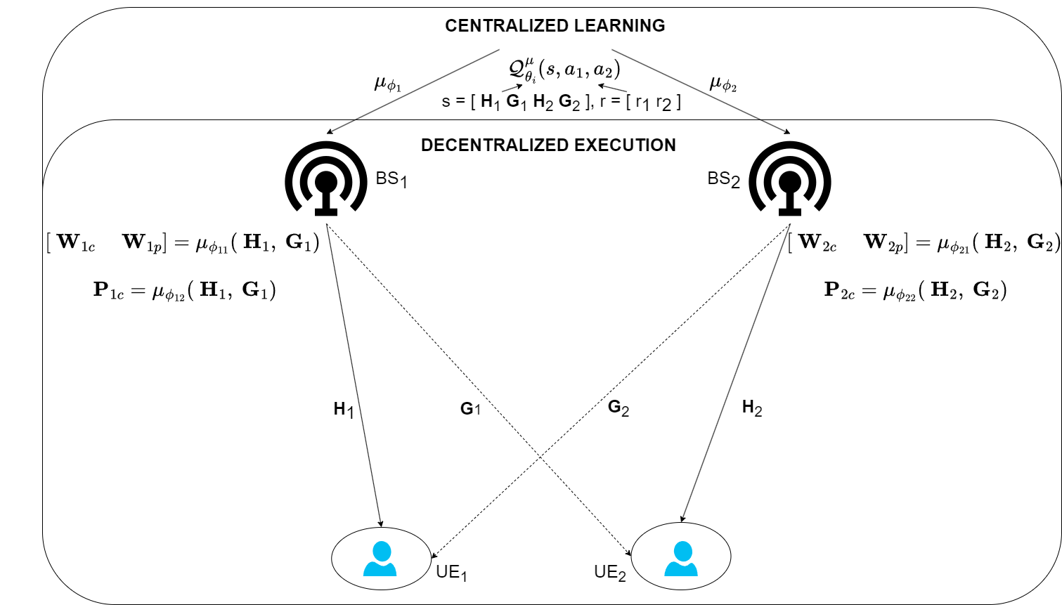
MADDPG employs centralized training and decentralized execution, where all agents share a common critic network to facilitate joint action optimization, and decentralized execution, where each agent independently executes its learned policy based on local observations. Specifically, the critic network in MADDPG takes as input not only the local observations and actions of an individual agent, but also the observations and actions of all other agents in the system. By doing so, the critic can learn a centralized value function that takes into account the joint actions of all agents. This centralized value function can then be used to train each agent’s policy network.

On the other hand, during execution or deployment, each agent only has access to its own local observations and actions, namely, agent $i$ at $BS_{i}$ chooses the precoding matrices $\bm{W}_{ic}$, $\bm{W}_{ip}$ and power allocation coefficient vectors $\bm{P}_{ic}$ (and inherently $\bm{P}_{ip}$) based on local information characterized by $\bm{H}_{i}$ and $\bm{G}_{i}$ only. This is known as decentralized execution, as each agent acts independently based on its own observations and policies without relying on information from other agents. By decoupling the execution from the learning, MADDPG is able to handle complex multi-agent systems, where agents have limited or incomplete information about the system as a whole.

Figure 2: MADDPG with RSMA algorithm structure for the MIMO case.

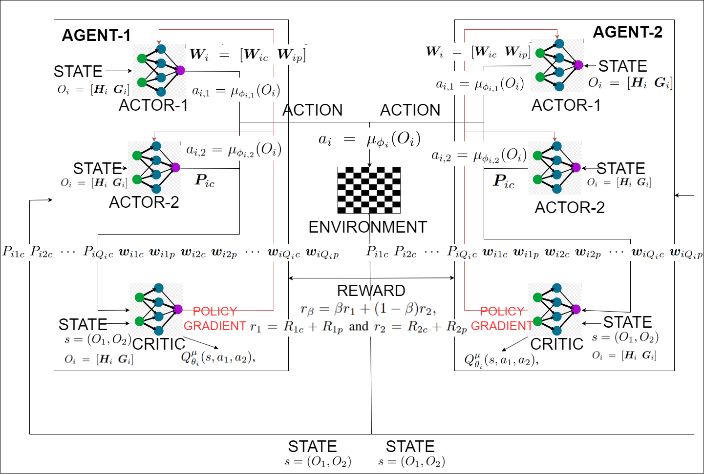
First, we assume a fixed decoding order. For each decoding order, we consider an environment with two agents. The overall system architecture is shown in Fig. 1 and the algorithm structure is summarized in Fig. 2. In this system, each agent $i$ at $BS_{i}$ chooses a precoding matrix $\bm{W}_{i}=[\bm{W}_{ic}~{}\bm{W}_{ip}]$ and a power allocation coefficient vector $\bm{P}_{ic}$ based on the local observation $O_{i}=[\bm{H}_{i}~{}\bm{G}_{i}]$, $i\in\{1,2\}$. We construct actor networks parameterized by $\phi_{i1}$ for the precoding vectors $\bm{w}_{ik}$, for $k=1,\ldots,Q_{i}$; and parameterized by $\phi_{i2}$ for the power allocation coefficients $P_{ikc}$, and a critic network to evaluate the performance of policies for each agent $i$. Please note that, for the single antenna case, actor network is only responsible for choosing $P_{ikc}$ for each agent since there is no need to determine $\bm{W}_{i}$. Let $\mu=\{\mu_{\phi_{11}}(O_{1}),\mu_{\phi_{12}}(O_{1}),\mu_{\phi_{21}}(O_{2}),\mu_{\phi_{22}}(O_{2})\}$ denote the set of policies parameterized by $\phi=\{\phi_{1},\phi_{2}\}$ where $\phi_{1}=\{\phi_{11},\phi_{12}\}$ and $\phi_{2}=\{\phi_{21},\phi_{22}\}$. The agents will choose their actions $a_{i}=[P_{i1c}~{}P_{i2c}~{}\cdots~{}P_{iQ_{i}c}~{}\bm{w}_{i1c}~{}\bm{w}_{i1p}~{}\bm{w}_{i2c}~{}\bm{w}_{i2p}~{}\cdots~{}\bm{w}_{iQ_{i}c}~{}\bm{w}_{iQ_{i}p}]$ according to the partial state $O_{i}$ by following a deterministic policy $a_{i}=\mu_{\phi_{i}}(O_{i})$. To ensure sufficient exploration, we also add a noise vector, whose entries are independent and identically distributed according to $\mathcal{N}(0,\,\sigma_{N}^{2})$ to the deterministic action $a_{i}=\mu_{\phi_{i}}(O_{i})$. Then, the gradient of the expected reward $J(\phi_{i})$ for each agent $i$ can be computed as

$$\nabla_{\phi_{i}}J(\phi_{i})=\mathbb{E}\left[\nabla_{a_{i}}\mathcal{Q}_{\theta_{i}}^{\mu}(s,a_{1},a_{2})|_{a_{i}=\mu_{\phi_{i}}(O_{i})}\nabla_{\phi_{i}}\mu_{\phi_{i}}(O_{i})\right],$$ (17)

where $\mathcal{Q}_{\theta_{i}}^{\mu}(s,a_{1},a_{2})$ represents the state action value function parameterized by the critic network with $\theta_{i}$ for each agent. It takes as input the state information $s=(O_{1},O_{2})$; i.e., channel gains for all users, and the actions $a=(a_{1},a_{2})$ of all agents, and outputs the $\mathcal{Q}$-value for agent $i$.

Each agent receives a collaborative reward, denoted by $r_{\beta}$, which is a function of the environmental state and actions taken according to state observation.

$$r_{\beta}=\beta r_{1}+(1-\beta)r_{2},$$ (18)

where $r_{1}=R_{1c}+R_{1p}$ and $r_{2}=R_{2c}+R_{2p}$ for the case of RSMA, and $\beta$ and $1-\beta$ denote the given weights of the user rates, defined in (16a). MADDPG uses this rate expression to maximize the total discounted return, which is given by $\mathrm{R}=\sum_{t=0}^{\infty}\gamma^{t}r_{\beta,t}^{\mu}$ where $r_{\beta,t}^{\mu}$ is the average sum-rate reward obtained under policy $\mu$ at time $t$, and $\gamma\in[0,1]$ denotes the discount factor.

The critic network estimates the $\mathcal{Q}$-value function $\mathcal{Q}_{\theta_{i}}^{\mu}(s,a_{1},a_{2})$, which is the expected cumulative reward starting from state $s=(\bm{H}_{1},\bm{G}_{1},\bm{H}_{2},\bm{G}_{2})$ and taking a joint action $a$ under policies $\mu=\{\mu_{\phi_{1}},\mu_{\phi_{2}}\}$. MADDPG algorithm employs an experience replay buffer which records the experiences of all agents and stores tuples $<s,a_{1},a_{2},r_{\beta},s^{\prime}>$. A mini-batch of $B$ experience tuples ${<s_{j},a_{1,j},a_{2,j},r_{\beta,j},s^{\prime}_{j}>}_{j=1}^{B}$ are randomly sampled from the replay buffer $\mathcal{D}$, where $s^{\prime}_{j}=(O^{\prime}_{1,j},O^{\prime}_{2,j})$ and $r_{\beta,j}$ denote the next state and reward observed after actions $a_{1,j}$, $a_{2,j}$ are taken at state $s_{j}=(O_{1,j},O_{2,j})$, respectively.

In addition, target networks from the DQN algorithm [36] are adopted to provide stability between actor and critic updates. Target actor networks and critic networks are denoted by $\mu^{-}$ and $Q^{-}$ and parameterized by $\phi^{-}$ and $\theta^{-}$, respectively.

We update the critic network by minimizing the mean-squared temporal difference (TD) error $\mathcal{L}(\theta_{i})$ in sampled mini-batch.

$$\mathcal{L}(\theta_{i})=\frac{1}{B}\sum_{j=1}^{B}\left(y_{j}-\mathcal{Q}_{\theta_{i}}^{\mu}(s_{j},a_{1,j}a_{2,j})\right)^{2},$$ (19)

where the TD target $y_{j}$ is computed as

$$\begin{split}y_{j}&=r_{\beta,j}+\gamma\mathcal{Q}_{\theta_{i}}^{\mu^{-}}(s^{\prime}_{j},\mu_{\phi^{-}_{1}}(o^{\prime}_{1,j}),\mu_{\phi^{-}_{2}}(o^{\prime}_{2,j})).\end{split}$$ (20)

Then, we update the actor network for each agent $i$ by using the deterministic policy gradient as

$$\nabla_{\phi_{i}}J(\phi_{i})\approx\frac{1}{B}\sum_{j=1}^{B}\nabla_{a_{i}}\mathcal{Q}_{\theta_{i}}^{\mu}(s_{j},a_{1,j},a_{2,j})\nabla_{\phi_{i}}\mu_{\phi_{i}}(O_{i}).$$ (21)

The target networks are then updated softly to match actor and critic parameters

$$\phi^{-}_{i} \leftarrow\tau\phi_{i}+(1-\tau)\phi^{-}_{i}\ \theta^{-}_{i} \leftarrow\tau\theta_{i}+(1-\tau)\theta^{-}_{i},$$ (22)

where $0<\tau<1$ is a hyper-parameter controlling the update rate. Finally, we select the best sum-rate over all decoding orders for exhaustive search case.

The MADDPG with rate-splitting for interference channels is also detailed in Algorithm 1. The hyperparameters of the algorithm are tuned experimentally for the sum-rate maximization problem and are outlined in Table II.

In the next subsection, we enhance the MADDPG algorithm by incorporating decoding order optimization rather than employing exhaustive search. The efficacy of this approach will be demonstrated in Section V.

III-A Decoding Order Optimization

In multi-user systems, RSMA utilizes a decoding order through SIC, crucial for determining achievable transmission rates. The decoding order is directly related with the point achieved on the rate region. Therefore, determining the optimal decoding order is also crucial to achieve higher rates. Once the optimal decoding order is determined by the MADDPG framework, this information can be conveyed to the receivers in a few bits, without harming the overall communication rate.

To estimate the optimal decoding order, which maximizes the sum-rate, an additional actor network is introduced to the multi-agent system. Let $\eta_{i}$ denote the decoding order for ${UE}_{i}$, $i=1,2$. In a scenario with two base stations and two users, where ${UE}_{i}$ faces two possible choices based on the decoding order, as specified in (6). Here, the variable $\eta_{i}$ takes values of either $0$ or $1$, where $0$ corresponds to option (b), and $1$ corresponds to the decoding order indicated in option (a) in (6).

The new actor network is parameterized by $\phi_{0}$ and designed to share the same state space and reward function as the existing ones (18). It observes the state $s=(\bm{H}_{1},\bm{G}_{1},\bm{H}_{2},\bm{G}_{2})$ and chooses the decoding order $\eta_{i}$ for both UEs following the deterministic policy $\mu_{\phi_{0}}(s)$. In this specific scenario, agents extends their decision-making to include additional actions and the new set of joint action becomes $a=[P_{1c}~{}P_{2c}~{}\bm{W}_{1c}~{}\bm{W}_{1p}\bm{W}_{2c}~{}\bm{W}_{2p}~{}\eta_{1}~{}\eta_{2}]$. Following this decision-making process, each agent is rewarded collaboratively. The collaborative reward is determined by the specific decoding order chosen, the environmental state, and the additional actions taken by the agents.

Algorithm 1 MADDPG with RSMA for Weighted Sum-Rate Maximization

Initialize actor networks $\mu_{{\phi_{i}}}(O_{i})$ and critic networks $\mathcal{Q}_{\theta_{i}}(s_{i},a_{i,1},a_{i,2})$ with weights $\theta_{i}$ and $\phi_{i}$

Initialize target networks $\mu^{-}$ and $\mathcal{Q}^{-}$ with weights $\theta^{-}_{i}\leftarrow\theta_{i}$ and $\phi^{-}_{i}\leftarrow\phi_{i}$

Initialize replay buffer $\mathcal{D}$

for $episode=1,\ldots,E$ do

    for $t=1,\ldots,T$ do

         for each agent $i$ do

             Observe partial state $O_{i}=(\bm{H}_{i},\bm{G}_{i})$

             Select action $a_{i}=\mu_{\phi_{i}}(O_{i})$,

             Execute action with exploration noise:

             $\quad a_{i}=\mu_{\phi_{i}}(O_{i})+\mathcal{N}(0,\,\sigma_{N}^{2})$.

             Observe reward $r_{i}$.

         end for

         Observe:

             the sum-rate reward $r_{\beta}=\beta r_{1}+(1-\beta)r_{2}$,

             state $s=(O_{1}~{}O_{2})=(\bm{H}_{1},\bm{G}_{1},\bm{H}_{2},\bm{G}_{2})$ and

             next state $s^{\prime}$

         Add transition $(s,a_{1},a_{2},r_{\beta},s^{\prime})$ to $\mathcal{D}$

         Sample a minibatch of $B$ transitions:

         $\quad(s_{j},a_{1,j},a_{2,j},r_{\beta,j},s_{j}^{\prime})$ from $\mathcal{D}$

         Compute target action:

         $\quad a^{\prime}_{j}=\mu^{-}(o^{\prime}_{j})$

         Compute target Q-value:

         $\quad y_{j}=r_{\beta,j}+\gamma\mathcal{Q}^{-}(s^{\prime}_{j},a^{\prime}_{1,j},a^{\prime}_{2,j})$

         Update each critic by minimizing the loss:

         $\quad L(\theta_{i})=\frac{1}{B}\sum_{j=1}^{B}(y_{j}-\mathcal{Q}_{\theta_{i}}^{\mu}(s_{j},a_{i,1},a_{i,2}))^{2}$

         Update each actor using the sampled policy gradient:

         $\quad\nabla_{\phi_{i}}J(\phi_{i})\approx\frac{1}{B}\sum_{j=1}^{B}\nabla_{a_{i}}\mathcal{Q}_{\theta_{i}}^{\mu}(s_{j},a_{1,j},a_{2,j})\nabla_{\phi_{i}}\mu_{\phi_{i}}(O_{i})$

         Soft update target networks:

         $\quad~{}~{}\theta^{-}_{i}\leftarrow\tau\theta_{i}+(1-\tau)\theta^{-}_{i},~{}~{}\phi^{-}_{i}\leftarrow\tau\phi_{i}+(1-\tau)\phi^{-}_{i}$

    end for

end for

III-B Imperfect Channel State Information

In this subsection, channel estimation errors, a practical consideration in real-world scenarios, is systematically explored. The examination of these errors encompasses two distinct modalities: the first, wherein the estimation error remains the same irrespective of the SNR value, and the second, where the estimation error decreases with increasing SNR. The estimated channels can be represented as

$$\tilde{\bm{H}}_{i}=\bm{H}_{i}+\bm{E}_{i},\quad\tilde{\bm{G}}_{j}=\bm{G}_{j}+\hat{\bm{E}}_{j}$$ (23)

where the resulting estimation error terms, denoted by $\bm{E}_{i}$ and $\hat{\bm{E}}_{j}$, arise from the disparity between the estimated channel coefficients, represented by $\tilde{\bm{H}}_{i}$ and $\tilde{\bm{G}}_{j}$, and the actual channel coefficients denoted as $\bm{H}_{i}$ and $\tilde{\bm{G}}_{j}$. It is important to note that the matrices $\bm{E}_{i}$, $\bm{H}_{i}$, and $\tilde{\bm{H}}_{i}$ all belong to the complex field and have dimensions $N_{i}\times M_{i}$; i.e. $\mathbb{C}^{N_{i}\times M_{i}}$. In the case of varying imperfections, each entry $[\bm{E}_{i}]{(x,y)}$, $x=1,\ldots,N_{i}$, $y=1,\ldots,M_{i}$, is determined as $\frac{SNR^{-0.6}}{5}\mathcal{CN}(0,\sigma^{2})$, where $\sigma^{2}=1$. Similarly, the matrices $\hat{\bm{E}}_{j}$, $\bm{G}_{j}$, and $\tilde{\bm{G}}_{j}$ are all in $\mathbb{C}^{N_{i}\times M_{j}}$, $i\neq j$. Each entry in $\hat{\bm{E}}_{i}$ is drawn from $\frac{SNR^{-0.6}}{5}\mathcal{CN}(0,\sigma^{2})$ with $\sigma^{2}=1$. In the case of fixed channel estimation errors, each entry in $\bm{E}_{i}$ or $\hat{\bm{E}}_{j}$ will be distributed according to $\frac{SNR^{-0.6}}{5}\mathcal{CN}(0,\sigma^{2})$ with $\sigma^{2}=1$ in Section V.

It is crucial to highlight that the estimation error solely influences the computation of precoders, while the rates are computed employing the exact channel coefficients. The actor network in each agent incorporates estimated channel coefficients, whereas the reward function is formulated based on the exact channel coefficients.

TABLE II: Hyperparameters of MADDPG algorithm for MIMO

Parameter	Value	Parameter	Value
discount factor $\gamma$	0.99	optimizer	Adam
minibatch size $B$	128	loss function	MSE loss
replay memory length $D$	15000	no. of connected layers	5
activation function	ReLU	learning rate	$5\times 10^{-5}$
hidden size	64	episode length $T$	200
update rate $\tau$	0.01	exploration noise $\sigma_{N}^{2}$	0.1
number of episodes $E$	12000	weight of user rates $\beta$	0.5

III-C MADDPG with no Rate-Splitting

If there is no rate-splitting, our scheme reduces to the one in [20]. In this case, there is no common message, $\bm{b}_{ic}=\emptyset$, and $\bm{W}_{ic}$ is an all zero matrix. The one in that for MADDPG without rate-splitting, (18) can be modified by using $r_{1}=R_{1}$ and $r_{2}=R_{2}$ that are given in (24) and (25). Also, since we only optimize precoders, but not $\bm{P}_{ikc}$, we use actions only for precoder evaluation. Then, the rates achieved by this scheme for the MIMO case become

$$R_{1}^{\pi} = \log_{2}\det\Bigl{(}\bm{I}_{N_{1}}+{(\bm{H}_{1}\bm{W}_{1}^{\pi}\bm{W}_{1}^{\pi,H}\bm{H}_{1}^{H})}$$ (24)

$$\qquad\quad{({{\bm{{G}}_{2}\bm{W}_{2}^{\pi}\bm{W}_{2}^{\pi,H}\bm{{G}}_{2}^{H}}+N_{0}\bm{I}_{N_{1}}})}^{-1}\Bigl{)}$$

$$R_{2}^{\pi} = \log_{2}\det\Bigl{(}\bm{I}_{N_{2}}+{(\bm{H}_{2}\bm{W}_{2}^{\pi}\bm{W}_{2}^{\pi,H}\bm{H}_{2}^{H})}$$ (25)

$$\qquad\quad{({{\bm{{G}}_{1}\bm{W}_{1}^{\pi}\bm{W}_{1}^{\pi,H}\bm{{G}}_{1}^{H}}+N_{0}\bm{I}_{N_{2}}})}^{-1}\Bigr{)}$$

where $\pi=\{drl\}$ indicates the precoders for MADDPG without rate-splitting.

IV Benchmark Precoding Schemes

In this section, we will be explaining the benchmark precoding schemes maximum ratio transmission (MRT) [37], zero-forcing (ZF) precoding [37], and leakage-based precoding [38]. We will also compare with the upper bounds [17, 16, 18] on interference channels.

IV-A Maximum Ratio Transmission

MRT is employed at the transmitter side, where transmit antenna weights are matched to the channel [37],[39]. This way, the maximum received SNR is attained at the intended receivers. This process takes advantage of the spatial diversity offered by multiple antennas at both the transmitter and receiver ends. By adjusting the transmission weights in this manner, MRT aims to maximize the received signal power, effectively exploiting the available spatial dimensions and enhancing the system’s overall performance in terms of reliability and data throughput. However, MRT does not take interference into consideration. In MRT there is no rate-splitting and there is no common message, $\bm{b}_{ic}=\emptyset$, $\bm{W}_{ic}$ is an all zero matrix, $\bm{W}_{i}^{mrt}=\bm{W}_{ip}$ and for the MIMO case the precoder expression is given as

$${\bm{W}_{i}^{mrt}}={\bm{H}_{i}^{H}}.$$ (26)

IV-B Zero-Forcing

As in MRT, there is no rate-splitting in ZF transmission, and the transmitters aim to eliminate interferences among data streams by setting the transmission weights such that there is no interference caused on the receiving antennas. This is achieved by using the pseudo-inverse of the channel matrix to create a null space for the interference; i.e., by projecting input data symbols on the null space of $\bm{G_{i}}$. By nullifying the interference, ZF seeks to improve the reliability of data transmission without causing mutual interference among the multiple antennas, thereby enhancing the overall system performance in terms of throughput and signal quality. However, ZF might be sensitive to noise and can lead to amplification of noise in the process of eliminating interference. As a result, for ZF $\bm{b}_{ic}=\emptyset$, $\bm{W}_{ic}$ is an all zero matrix, and $\bm{W}_{i}^{zf}=\bm{W}_{ip}$, where

$${\bm{W}_{i}^{zf}}={({\bm{G}_{i}^{H}}{\bm{G}_{i}})^{-1}}{\bm{H}_{i}^{H}}.$$ (27)

IV-C Leakage-based Precoding

SLNR precoding technique is designed to optimize signal transmission in multi-user communication systems by minimizing interference among users while considering the system’s noise. Unlike traditional SNR-based approaches, SLNR focuses on minimizing both interference and noise to enhance the overall signal quality. In SLNR precoding, the precoding matrix is computed to maximize the desired signal power while minimizing the interference caused to other users. It aims to maintain a high signal-to-leakage-plus-noise ratio for the intended receiver, hence reducing interference while considering the system noise level. This precoding strategy is particularly useful in multi-user scenarios where reducing interference among users is crucial to improve overall system performance. In other words, leakage is a measure of how much signal power leaks into the other users. In this precoding scheme, the aim is to maximize the SLNR [38].

For a MIMO system the $k$th column of ${\bm{W}_{i}^{slnr}}$, ${\bm{w}_{ik}^{slnr}}$, is equal to the eigenvector that corresponds to the largest eigenvalue of ${\left({(N_{0}\bm{I}+{\bm{G}_{ik}^{H}\bm{G}_{ik}})^{-1}\bm{H}_{ik}^{H}\bm{H}_{ik}}\right)}$ where $\bm{G}_{ik}$ and $\bm{H}_{ik}$ represent the $k$th column of $\bm{G}_{i}$ and $\bm{H}_{i}$ respectively.

IV-D Interference Channel Upper Bounds

In [16] and [17], the authors suggest upper bounds for single antenna interference channels. For the single antenna case, we will use the upper bound given in [17, (58)-(71)] for weak and mixed interference conditions. In this context, for $i=1,2$, let $\bm{H}_{i}=h_{i}$ and $\bm{G}_{j}=g_{j}$. Then, the signal-to-noise ratio (SNR) of user $i$, $\mathrm{SNR}_{i}$, and interference-to-noise ratio (INR) for ${UE}_{i}$ caused by $UE_{j}$, $\mathrm{INR}_{i}$, of [17, (58)-(71)] respectively become $\mathrm{SNR}_{i}=\left|h_{i}\right|^{2}P_{i}/N_{0}$ and $\mathrm{INR}_{i}=\left|g_{j}\right|^{2}P_{j}/N_{0}$. Furthermore, the weak interference condition is defined as $\mathrm{INR}_{1}<\mathrm{SNR}_{2}$ and $\mathrm{INR}_{2}<\mathrm{SNR}_{1}$, while the mixed interference condition encompasses scenarios where either $\mathrm{INR}_{1}\geq\mathrm{SNR}_{2}$ and $\mathrm{INR}_{2}<\mathrm{SNR}_{1}$ or $\mathrm{INR}_{1}<\mathrm{SNR}_{2}$ and $\mathrm{INR}_{2}\geq\mathrm{SNR}_{1}$. Finally, the strong interference condition occurs, when $\mathrm{INR}_{1}>\mathrm{SNR}_{2}$ and $\mathrm{INR}_{2}>\mathrm{SNR}_{1}$. The interference channel becomes equivalent to a compound multiple access channel, in which both users decode all messages. In this case the symmetric rate point is given in [17, (33)] and the whole region is expressed in [16, (5)].

With these definitions, for each channel realization, we first determine whether the channel is a weak, mixed or strong interference channel and then directly apply the corresponding bounding equations in [17, (58)-(71)] or [16, (5)] for the SISO case.

When some of the devices have multiple antennas, the above bounds are not directly applicable and we adapt the upper bound calculated in [18]. For a comprehensive presentation, we present the bound as follows:

$$R_{1} \leq\log_{2}\operatorname{det}\left[\bm{I}_{N_{1}}+\rho_{11}\bm{H_{1}}\bm{H_{1}}^{H}\right]$$

$$R_{2} \leq\log_{2}\operatorname{det}\left[\bm{I}_{N_{2}}+\rho_{22}\bm{H_{2}}\bm{H_{2}}^{H}\right]$$

$$R_{1}+R_{2} \leq\log_{2}\operatorname{det}\left[\bm{I}_{N_{2}}+\rho_{12}\bm{G_{1}}\bm{G_{1}}^{H}+\rho_{22}\bm{H_{2}}\bm{H_{2}}^{H}\right]$$

$$+\log_{2}\operatorname{det}\left[\bm{I}_{N_{1}}+\rho_{11}\bm{H_{1}}\bm{K_{1}}\bm{H_{1}}^{H}\right]$$

$$R_{1}+R_{2} \leq\log_{2}\operatorname{det}\left[\bm{I}_{N_{1}}+\rho_{21}\bm{G_{2}}\bm{G_{2}}^{H}+\rho_{11}\bm{H_{1}}\bm{H_{1}}^{H}\right]$$

$$+\log_{2}\operatorname{det}\left[\bm{I}_{N_{2}}+\rho_{22}\bm{H_{2}}\bm{K_{2}}\bm{H_{2}}^{H}\right]$$

$$R_{1}+R_{2} \leq\log_{2}\operatorname{det}\left[\bm{I}_{N_{1}}+\rho_{21}\bm{G_{2}}\bm{G_{2}}^{H}+\rho_{11}\bm{H_{1}}\bm{K_{1}}\bm{H_{1}}^{H}\right]$$

$$+\log_{2}\operatorname{det}\left[\bm{I}_{N_{2}}+\rho_{12}\bm{G_{1}}\bm{G_{1}}^{H}+\rho_{22}\bm{H_{2}}K_{2}\bm{H_{2}}^{H}\right]$$

$$2R_{1}+R_{2} \leq\log_{2}\operatorname{det}\left[\bm{I}_{N_{1}}+\rho_{21}\bm{G_{2}}\bm{G_{2}}^{H}+\rho_{11}\bm{H_{1}}\bm{H_{1}}^{H}\right]$$

$$+\log_{2}\operatorname{det}\left[\bm{I}_{N_{1}}+\rho_{11}\bm{H_{1}}\bm{K_{1}}\bm{H_{1}}^{H}\right]$$

$$+\log_{2}\operatorname{det}\left[\bm{I}_{N_{2}}+\rho_{12}\bm{G_{1}}\bm{G_{1}}^{H}+\rho_{22}\bm{H_{2}}\bm{K_{2}}\bm{H_{2}}^{H}\right]$$

$$R_{1}+2R_{2} \leq\log_{2}\operatorname{det}\left[\bm{I}_{N_{2}}+\rho_{12}\bm{G_{1}}\bm{G_{1}}^{H}+\rho_{22}\bm{H_{2}}\bm{H_{2}}^{H}\right]$$

$$+\log_{2}\operatorname{det}\left[\bm{I}_{N_{2}}+\rho_{22}\bm{H_{2}}\bm{K_{2}}\bm{H_{2}}^{H}\right]$$

$$+\log_{2}\operatorname{det}\left[\bm{I}_{N_{1}}+\rho_{21}\bm{G_{2}}\bm{G_{2}}^{H}+\rho_{11}\bm{H_{1}}\bm{K_{1}}\bm{H_{1}}^{H}\right]$$ (28)

where

$$\bm{K}_{i} = \left(\bm{I}_{M_{i}}+\rho_{ij}\bm{G_{i}}^{H}\bm{G_{i}}\right)^{-1},\quad 1\leq i\neq j\leq 2$$ (29)

$$\rho_{ii} = \frac{\operatorname{Tr}\left(\bm{H_{i}}\bm{\mathbb{Q}_{i}}\bm{H_{i}}^{H}\right)}{N_{i}},\quad i=1,2,$$ (30)

$$\rho_{ij} = \frac{\operatorname{Tr}\left(\bm{G_{i}}\bm{\mathbb{Q}_{i}}\bm{G_{i}}^{H}\right)}{N_{i}},\quad 1\leq i\neq j\leq 2.$$ (31)

Finally, the covariance matrix is represented as $\bm{\mathbb{Q}_{i}}=\mathbb{E}\left(\bm{x_{i}}\bm{x_{i}}^{H}\right)$.

IV-E No Interference

For this case, interference terms are assumed to be 0 to obtain a trivial upper-bound. The rates achieved by each user for a MIMO system is then written as

$$R_{1}=\log\det\left(\bm{I}_{N_{1}}+{(\bm{H}_{1}\bm{W}_{1}\bm{W}_{1}^{H}\bm{H}_{1}^{H})N_{0}^{-1}}\right),$$ (32)

$$R_{2}=\log\det\left(\bm{I}_{N_{2}}+(\bm{H}_{2}\bm{W}_{2}\bm{W}_{2}^{H}\bm{H}_{2}^{H})N_{0}^{-1}\right).$$ (33)

V Simulation Results

In this section, we delve into an exhaustive examination of simulation results for MADDPG with RSMA. This method is meticulously compared against its subset, the MADDPG with no rate-splitting [20], offering valuable insights into the role of rate-splitting in shaping the overall performance. Moreover, we extend our investigation to encompass a comprehensive set of benchmark schemes outlined in Section IV, covering a spectrum of scenarios including SISO, MISO and MIMO configurations. This extensive analysis allows us to examine the proposed scheme’s adaptability and efficacy across diverse communication scenarios.

Our primary objective is to maximize the weighted sum-rate in a two-user interference channel by optimizing both the power allocation coefficients and the precoders. Maximizing the sum-rate in RSMA is crucial as it directly correlates with the overall efficiency and throughput of the communication system. A higher sum-rate implies the ability to transmit more information per unit time. The MADDPG algorithm provides a framework for the coordinated learning of multiple agents to optimize the sum-rate. MADDPG enables these agents to adapt their strategies collaboratively, ensuring a balanced and effective allocation of resources, such as power and decoding orders, to maximize the sum-rate. This optimization process, particularly in the context of RSMA, introduces inherent complexities. The nature of RSMA, with its simultaneous consideration of common and private streams, renders traditional optimization approaches less effective, making the utilization of reinforcement learning approaches appealing. In addition to maximizing the sum-rate, our study will delve into the performance implications of decoding order estimation. Furthermore, we will rigorously examine the system’s resilience in the face of channel estimation errors, a crucial consideration in practical communication scenarios. This multifaceted exploration aims to provide a thorough understanding of the proposed model’s capabilities, particularly in the complex landscape of RSMA.

The instantiation of the MADDPG algorithm was conducted within the PyTorch 1.9.1 framework. The training architecture incorporates four fully connected layers for both the critic and the actors, providing a robust and sophisticated foundation for the learning process. To assess the algorithm’s convergence, extensive monitoring was conducted over 12,000 episodes for MIMO, 4,000 episodes for MISO, and 2,400 episodes for SISO cases, with each episode consisting of 200 time steps. This comprehensive evaluation resulted in the acquisition of rates across varying SNR scenarios. Within the simulated environment, the channel coefficients $\bm{H}_{i}$, and $\bm{G}_{i}$ for $i=1,2$ are assumed to follow an independent and identically distributed circularly symmetric complex Gaussian distribution with zero mean and unit variance. Irrespective of the antenna configuration, be it SISO, MISO, or MIMO, the total power $P_{i}$ in (16c) is consistently set to 1.

Our investigation will encompass a comprehensive analysis of our communication scheme across diverse SNR regimes, specifically considering the case where SNR is defined as the reciprocal of the noise power $N_{0}$ (i.e., SNR = 1/$N_{0}$), given that the signal power $P_{i}$ is fixed at 1. To maintain uniformity and adhere to power constraints, the precoders employed in each scheme will undergo normalization by their respective magnitudes. This normalization process ensures that the power constraints are consistently satisfied across various SNR scenarios, facilitating a systematic evaluation of the scheme’s performance under different SNR conditions.

Figure 3: Average sum-rate achieved by MADDPG and the upper bound due to [16] and [17] for $M=1$ and $Q=1$. The MADDPG curves are obtained by averaging 25 runs, each having 200 time steps after the algorithm achieves convergence.

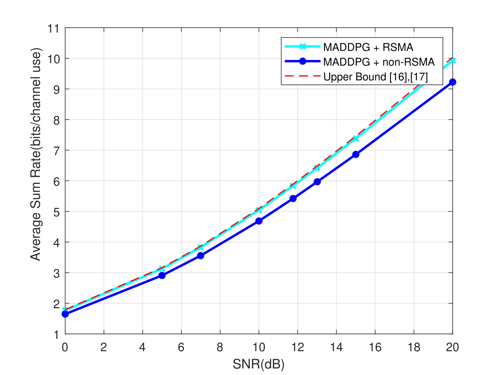
Fig. 3 illustrates the average sum-rate as a function of SNR for the two-user interference channel for the SISO case; i.e. $M_{i}=1$, $N_{i}=1$, $i=1,2$. The objective is to discern the impact of rate-splitting on performance. The plot includes curves for the MADDPG algorithm both with and without rate-splitting, alongside the upper bound elucidated in Section IV. The MADDPG + RSMA curves are derived from averaging 25 runs, each consisting of 200 time steps, post-convergence of the algorithm. Notably, the results indicate that MADDPG with rate-splitting can attain the upper bound, signifying its efficacy in approaching theoretical limits. Furthermore, as SNR increases, the disparity between the performances of MADDPG with and without rate-splitting becomes more pronounced. This observation underscores the significance of rate-splitting as a strategic mechanism for augmenting the sum-rate, particularly in scenarios characterized by high SNR.

Figure 4: Average sum-rate achieved by MADDPG and the benchmark schemes for $M=3$ and $Q=1$. The MADDPG curves are obtained by averaging 50 runs, each having 1000 time steps after the algorithm achieves convergence.

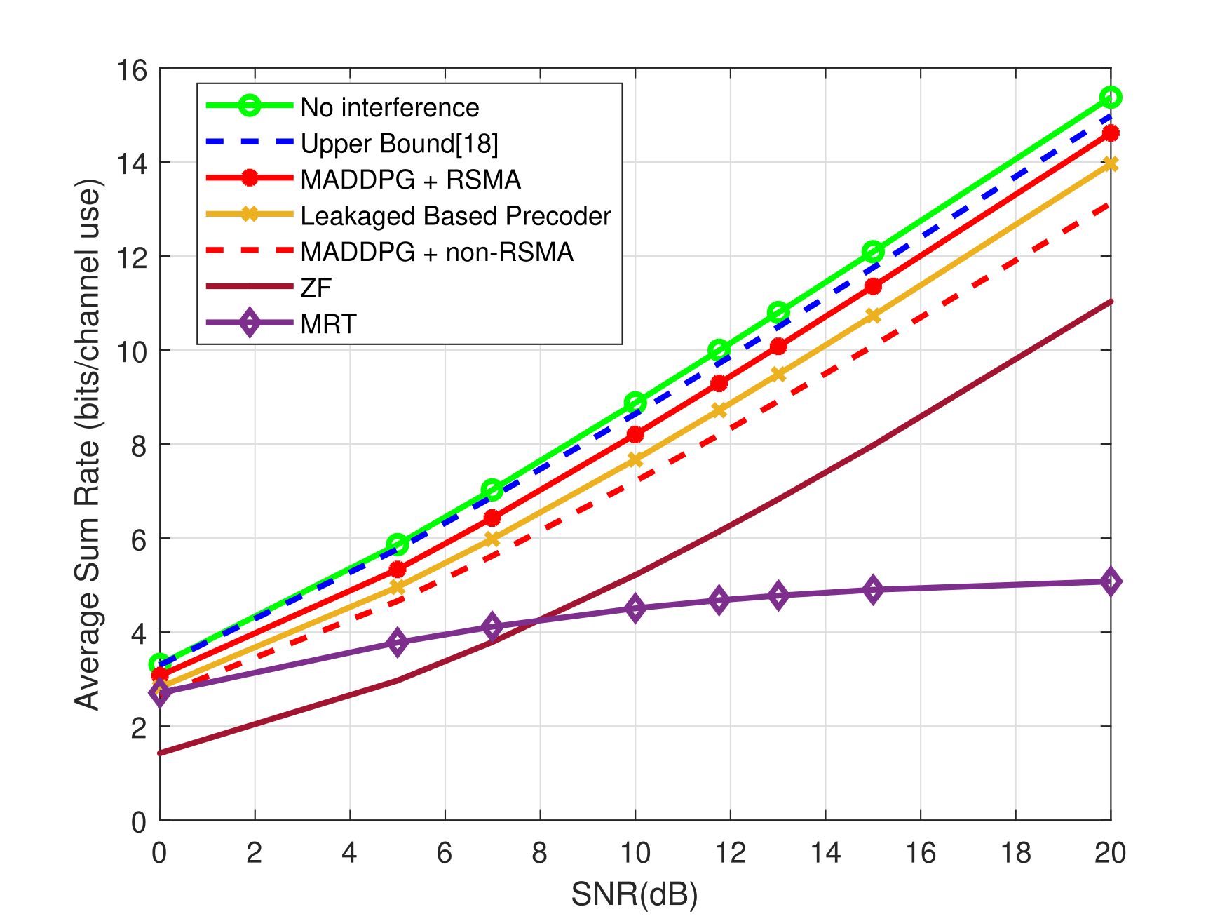
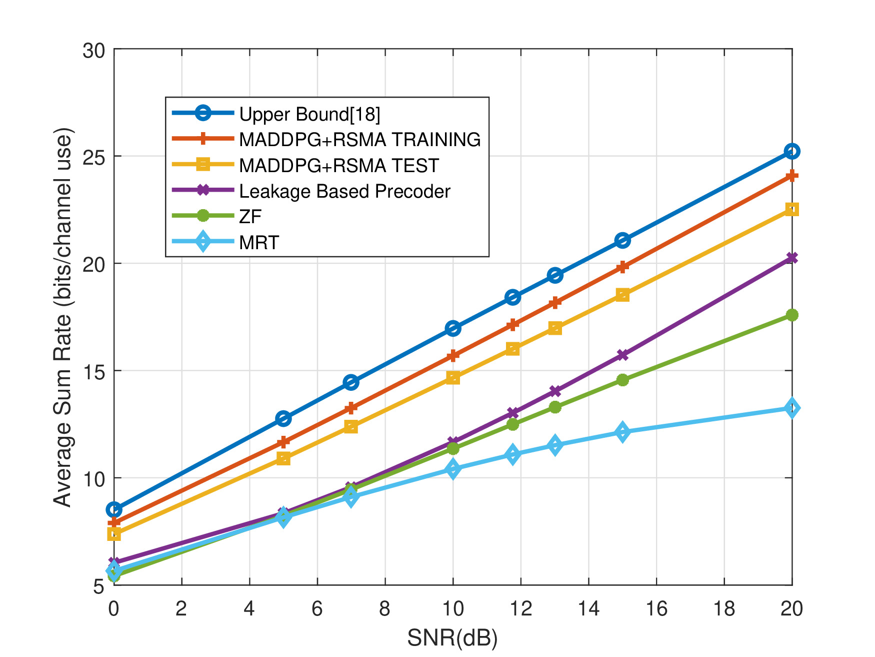
In Fig. 4, we present a detailed analysis of the average sum-rate results for $M=3$ and $Q=1$. The comparison involves multiple schemes, including MADDPG with and without rate-splitting, MRT, ZF, and leakage-based precoding. Additionally, the upper bound, as defined in [18], serves as a reference for assessing the performance achieved by the proposed approach. The case where there is no interference is also shown as an additional reference. Analyzing the results, it is evident that MADDPG with rate-splitting is very close to the upper bound. When compared with its no rate-splitting counterpart, we observe 2 dB gain when SNR is 12 dB or higher. MADDPG with RSMA also exhibits superior performance compared to MRT, ZF, and leakage-based precoding. MRT experiences challenges in the presence of severe interference, leading to a convergent behavior rather than maintaining an increasing average sum-rate curve. On the other hand, ZF, while immune to interference, struggles to achieve sufficiently high signal power, resulting in limited performance. Leakage-based precoding strikes a balance between desired signal power and leaking interference power, leading to higher rates than both MRT and ZF.

The unique advantages of MADDPG with rate-splitting become apparent in the above comparison. Firstly, MADDPG utilizes the SINR as a metric, which is a more relevant than SLNR or SNR. Secondly, the incorporation of rate-splitting enables MADDPG to intelligently manage interference. In scenarios with weak interference, more power is allocated to private messages, while in the presence of strong interference, common messages are transmitted with higher power. The consideration of all possible decoding orders further enhances the adaptability of MADDPG with rate-splitting, resulting in superior performance compared to benchmark schemes. This comprehensive analysis sheds light on the nuanced benefits and capabilities of the proposed approach in addressing interference challenges in multi-antenna scenarios.

In Fig. 5 we present a detailed analysis of the average sum-rate results for $M=3$ and $Q=3$. Our proposed MADDPG with RSMA method consistently outperforms benchmark schemes ZF, MRT, and leakage-based precoder. This superiority can be attributed to the unique advantages offered by RSMA. By intelligently allocating power and managing interference, RSMA ensures more efficient resource utilization, resulting in enhanced overall system performance. Unlike in SISO, we also observe a gap between the training and test performance for MADDPG with RSMA. This increasing gap can be attributed to the growing number of parameters that need to be estimated as we move to more complex antenna configurations. Additionally, when compared with Fig. 3 and Fig. 4 the gap between the upper bound and the MADDPG with RSMA is wider. However, we note that this gap can occur if the upper bound in [18] is not tight for increasing number of transmit or receive antennas.

Figure 5: Average sum-rate achieved by MADDPG and the benchmark schemes for $M=3$, and $Q=3$. The MADDPG curves are obtained by averaging 5 runs, each having 200 time steps after the algorithm achieves convergence.

It is also important to note that, examining the number of training episodes across SISO, MISO, and MIMO configurations, a consistent upward trend was observed. This escalation in training episodes is a consequence of the heightened complexity inherent in transitioning from SISO to MIMO configurations. The increase in the number of antennas and parameters in the communication system demands more extensive training to optimize the reinforcement learning model effectively. The complexity of MIMO scenarios introduces additional intricacies, requiring the learning agent to navigate a larger action space and gain more information pertaining to the environment. Consequently, the iterative learning process is extended to accommodate the increased complexity and ensure the convergence of the reinforcement learning algorithm to an optimal policy. Therefore, the robustness and adaptability of our proposed method in the face of increasing complexity and interference make it a promising solution for advanced communication scenarios.

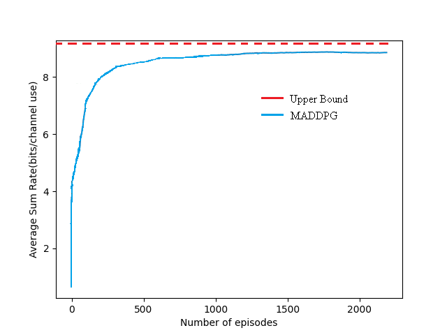
To examine the convergence behavior of the proposed algorithm in the MISO case with $M=3$ and $Q=1$, in Fig. 6, we present the average sum-rate versus the number of training episodes. For comparison, we include the upper bound[18] as well. The convergence curve depict the performance evolution of the MADDPG algorithm, providing a visual representation of its learning trajectory over the course of training episodes. This visual analysis not only facilitates an assessment of the algorithm’s convergence speed but also provides insights into how well the proposed solution converges towards the upper bound.

Figure 6: Convergence curve achieved by MADDPG for $M=3$ and $Q=1$ when $SNR=10$ dB. The convergence curve is obtained by averaging 50 runs, each having 1000 time steps given the number of training episodes.

Figure 7: Evolution of the weighted sum-rate for MADDPG with rate-splitting for $M=3$ and $Q=1$ when $SNR=10$ dB and for varying $\beta$ defined in (16a). The skip from one dot to the next represents 100 episodes of training, with the dots appearing after a delay of 500 episodes.

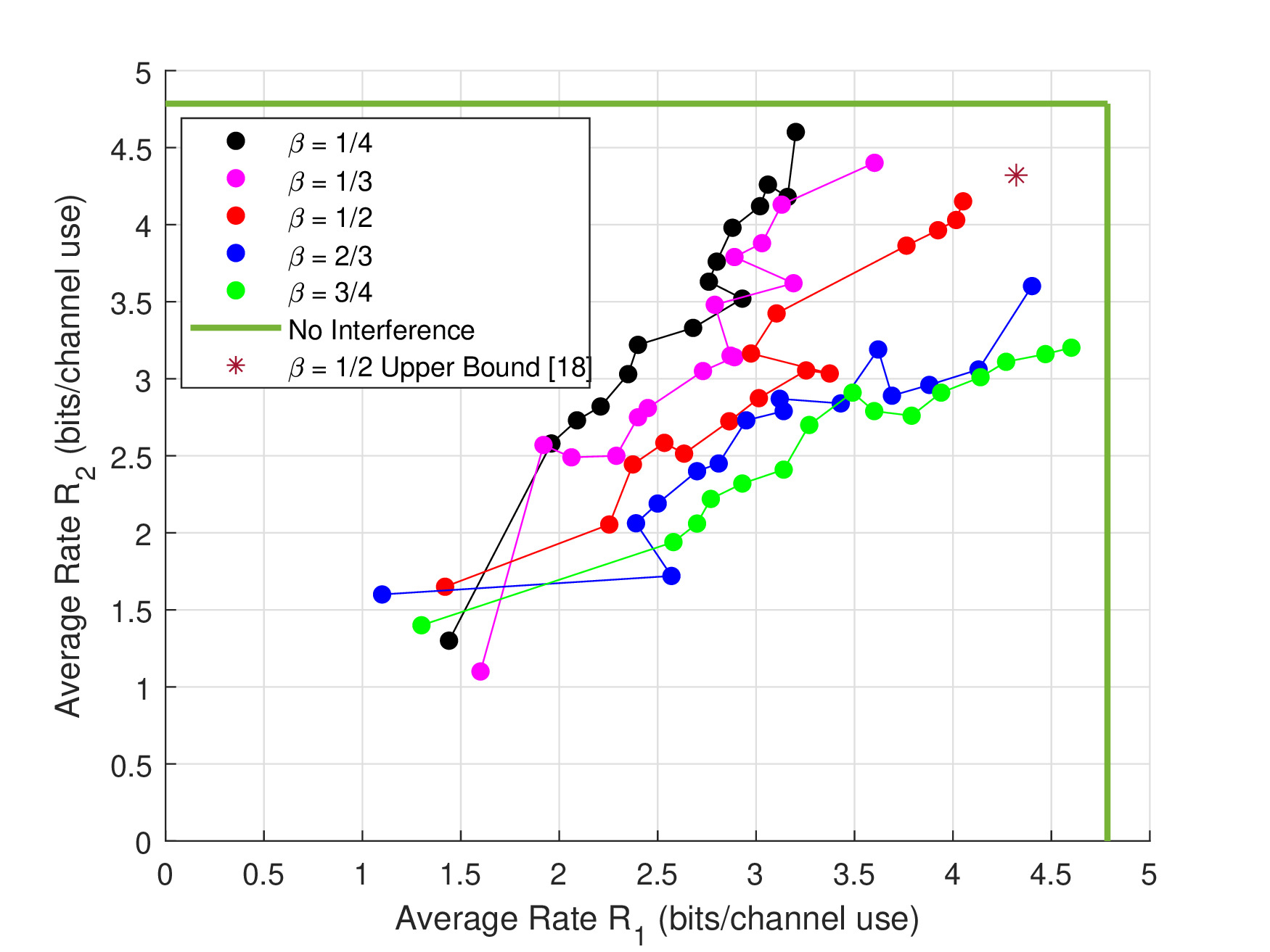
In Fig. 7, we illustrate the evolution of the weighted sum rate under a 10 dB SNR for $M=3$ and $Q=1$ for different weight parameter values; i.e. $\beta$ defined in (16a). In the figure, the skip from one dot to the next represents 100 episodes of training, with dots appearing after a delay of 500 episodes. The training process involves averaging our model over 100 runs, each comprising 1000 time steps realizations. The green outer box, corresponds to the no interference case, which is the ultimate upper bound for the achievable rate region. We also plot the upper bound [18] rate pair for $\beta=0.5$ with a star marker. The learning curve evolution analysis for different $\beta$ values allows us to explore how the rate region is obtained during the learning process. By observing how the system’s performance changes with different $\beta$ values, we gain insights into the algorithm’s behavior across a range of rate configurations, aiding in the assessment of its adaptability and responsiveness to changes in user rate priorities.

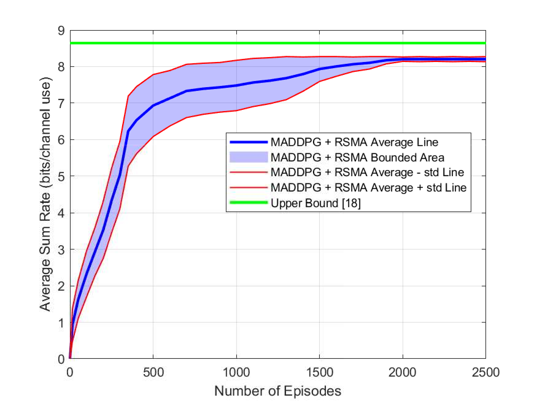
The confidence bounds of the reinforcement learning results are illustrated in Fig. 8. The figure, specifically obtained for the MADDPG with rate-splitting, showcase the robustness and reliability of the proposed approach. In assessing the performance of an algorithm, the inclusion of confidence bounds adds a layer of statistical significance to the obtained results. To calculate the confidence bounds, the results were averaged over 1000 runs, each comprising of 1000 time steps. Subsequently, the standard deviation of each run was computed. By adding and subtracting this standard deviation from the averaged line, a confidence bound was established. Comparison with the upper bound further contextualizes the reinforcement learning results, displaying the algorithm’s proximity to the theoretical performance limits. We also observe that after 2500 episodes, the algorithm consistently produces similar results. This stability and consistency in the performance indicate the robustness of our proposed solution. The algorithm’s ability to maintain comparable outcomes across multiple episodes highlights its reliability in handling the complexities of the MISO scenario. This robust behavior is crucial for ensuring dependable and consistent performance under varying conditions, contributing to its practical applicability and effectiveness in real-world settings.

Figure 8: Confidence bound achieved by MADDPG for $M=3$ and $Q=1$. The confidence interval are obtained by averaging 1000 runs, each having 1000 time steps given the number of training episodes.

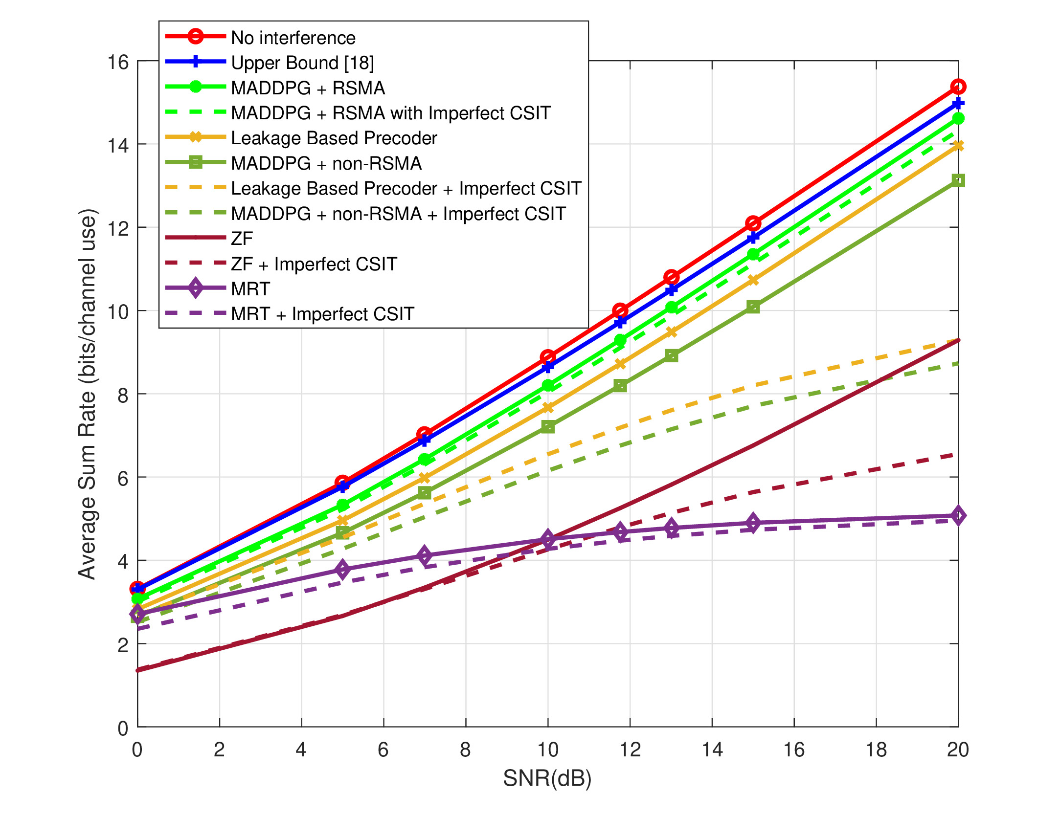
In Fig. 9, we systematically investigate the impact of a fixed value of imperfection over SNR, as defined in (23). The estimation error is set as $\frac{(10^{-0.6})}{5}\mathcal{CN}(0,\sigma^{2})$ with $\sigma^{2}=1$. In this analysis, the robustness of the proposed RSMA framework is highlighted. MADDPG with RSMA continues to follow the upper bound even under channel estimation errors. This quality becomes particularly pronounced when compared against alternative schemes, including ZF, MRT, leakage-based precoding, and non-rate-splitting MADDPG. In scenarios with imperfect channel state information at the transmitter (CSIT), the conventional schemes—ZF, MRT, leakage-based precoding, and non-rate-splitting MADDPG— encounter challenges in maintaining their performance due to their limited adaptability to variations in channel estimation errors. As channel estimation error variance is fixed with respect to SNR, the gap between perfect channel state knowledge and imperfect CSIT curves increase with increasing SNR for leakage based precoding, MADDPG with no rate-splitting and ZF. MRT relies on a straightforward strategy of amplifying the signals by the ratio of the received signal strength to the noise level, regardless of the specifics of the channel state. This approach minimizes the dependence on precise channel knowledge, making MRT less susceptible to the challenges associated with obtaining and utilizing accurate real-time channel state information. However, the simplicity that renders MRT resilient also contributes to its suboptimal nature. By adhering to a basic amplification strategy, MRT may not exploit the full potential of channel knowledge for optimizing transmission performance. However, the unique rate-splitting mechanism in MADDPG exhibits exceptional proficiency in alleviating the deleterious effects of channel estimation errors and continues to perform very close to the upper bound.

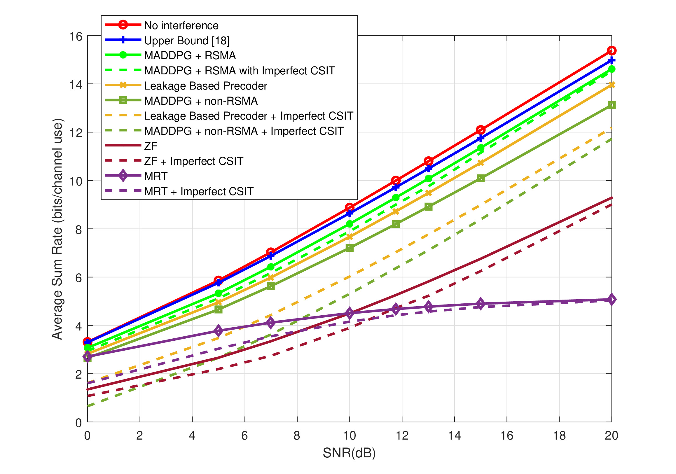
Additionally, Fig. 10 explores the scenario where imperfection varies according to $\frac{(SNR^{-0.6})}{5}\mathcal{CN}(0,\sigma^{2})$, with the same $\sigma^{2}=1$. Although a fixed channel estimation error is a more limiting assumption, this scenario is more practical. If SNR is high, it is very likely that it is high both for the channel estimation phase and for the data transmission phase. We observe that MADDPG with rate-splitting, ZF and MRT all converge with their imperfect CSIT versions for high SNR. MADDPG with no rate-splitting and leakage based precoder also converge but at very high SNR. Both Figs. 9 and 10 confirm the inherent resilience presented by RSMA, showcasing the superiority of the proposed framework under diverse SNR and channel estimation error conditions.

Figure 9: Effect of fixed channel estimation error on average sum rate versus SNR for $M=3$ and $Q=1$. The MADDPG curves are obtained by averaging 50 runs, each having 200 time steps after the algorithm achieves convergence.

Figure 10: Effect of variable channel estimation error on average sum rate versus SNR for $M=3$ and $Q=1$. The MADDPG curves are obtained by averaging 50 runs, each having 200 time steps after the algorithm achieves convergence.

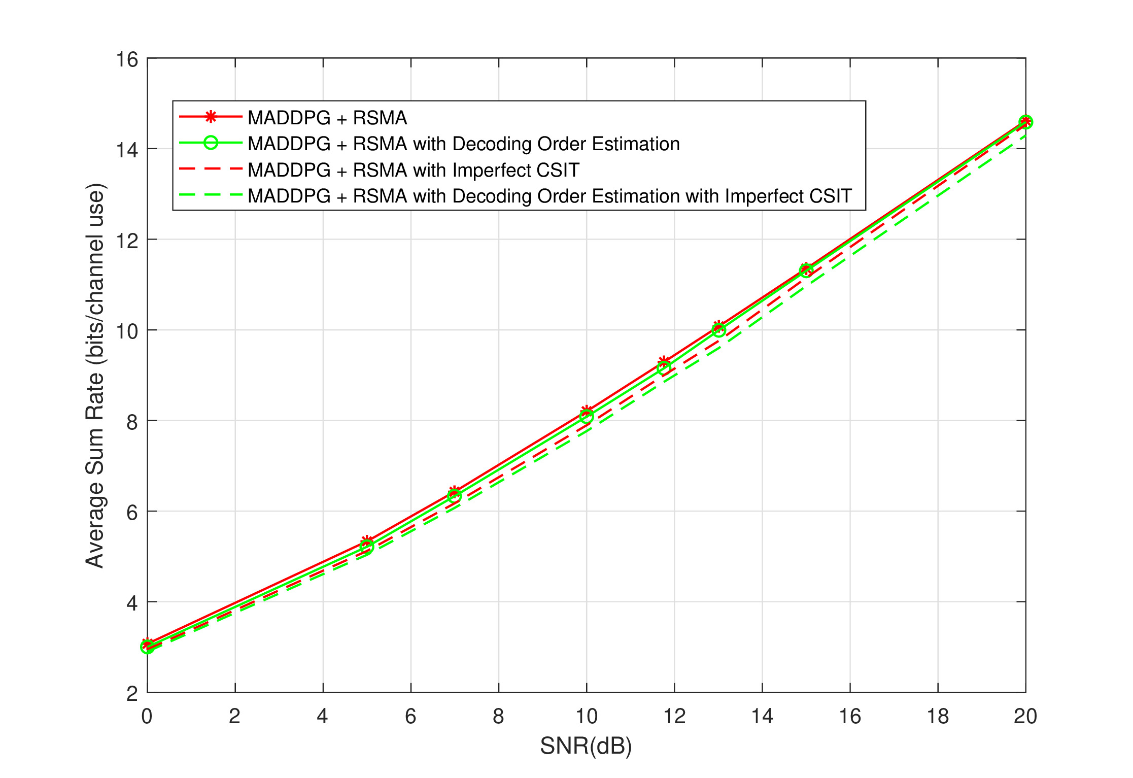
In Fig. 11, we study decoding order estimation. In the context of decoding order estimation, an additional actor network is introduced for each agent. Our investigation involves two key scenarios. Firstly, we examine the case where there is no channel estimation error. The second scenario considers the situation with a fixed value of channel estimation error over SNR, as defined earlier in this section. Remarkably, our findings reveal that decoding order estimation exhibits superior performance across all SNR values for both with and without channel estimation errors. This observation is particularly noteworthy as it shows the robustness and the efficacy of the proposed MADDPG framework. This result shows the ability of MADDPG to maintain superior performance even with decoding order estimation, addressing a crucial concern related to the complexity of RSMA, particularly in the SIC component. This suggests that by incorporating decoding order estimation, the system can achieve competitive performance while mitigating the associated complexity.

VI Conclusion and Future Work

In the context of advancing communication systems from 5G to 6G and beyond, rate-splitting multiple access has emerged as a notable transmission strategy. In rate-splitting, data streams are divided into common and private parts to strike the balance between treating interference as noise and decoding all unintended messages. However, especially in multiple antenna scenarios, finding the optimal precoders and transmit power levels for rate-splitting for all common and private data streams happens to be quite complex. To alleviate this issue, in this paper we propose computing the optimal precoders and transmit power levels for rate-splitting with deep reinforcement learning. Specifically, we use multi-agent deep deterministic policy gradient framework, in which decentralized agents with limited information collectively learn from a centralized critic to optimize actions in a multi-dimensional continuous policy space. This framework allows for centralized learning while enabling decentralized execution and offers a scalable and decentralized solution for interference management in multiple antenna environments. Simulation results demonstrate the effectiveness of our proposed rate-splitting method, achieving information-theoretical sum-rate upper bounds in single-antenna scenarios and impressive proximity to the upper bounds in multiple-antenna scenarios. Additionally, our method outperforms alternative approaches, zero-forcing, leakage-based precoding, and maximal ratio transmission, showcasing superior weighted sum-rate performance in both single and multiple antenna cases.

Figure 11: Average sum rate for MADDPG with decoding order estimation for $M=3$ and $Q=1$. The MADDPG curves are obtained by averaging 50 runs, each having 200 time steps after the algorithm achieves convergence.

Moreover, our work enhances the learning algorithm by addressing channel estimation errors and optimizing decoding order of common and private streams. Both aspects are important for prospective practical applications for improved robustness and efficiency. Especially, the latter is overlooked in the literature and generally a fixed decoding order is assumed at the receivers. Comparative analyses highlight the superiority of our approach, particularly in determining decoding orders and showing resilience against channel estimation errors. The investigation of learning curve evolution, variable weights in weighted sum rate calculation and confidence bounds complement our study for a comprehensive treatment of multi-agent deep deterministic policy gradient algorithm for rate-splitting.

Future work includes extending deep reinforcement learning models to handle scenarios with multiple users and designing new algorithms that take energy efficiency into account. Also, exploring hierarchical reinforcement learning approaches to tackle the complexity of rate-splitting optimization, and investigating meta-learning techniques to reduce the need for extensive training in new scenarios are of interest. In short, the future of using deep reinforcement learning for rate-splitting in wireless communications holds great potential for optimizing resource allocation, improving spectral and/or energy efficiency, and enabling more dynamic and adaptable wireless networks. Our work is a first step towards addressing these challenges and will lead to significant advancements in wireless communication systems.

References

- [1] O. N. Irkicatal, M. Yuksel, and E. T. Ceran, “Deep reinforcement learning aided rate-splitting for interference channels,” in IEEE Global Communications Conference, GLOBECOM, pp. 1–7, IEEE, 2023.
- [2] W. Jiang, B. Han, M. A. Habibi, and H. D. Schotten, “The road towards 6G: A comprehensive survey,” IEEE Open Journal of the Communications Society, vol. 2, pp. 334–366, 2021.
- [3] Y. Lu and X. Zheng, “6G: A survey on technologies, scenarios, challenges, and the related issues,” Journal of Industrial Information Integration, vol. 19, p. 100158, 2020.
- [4] M. U. A. Siddiqui, H. Abumarshoud, L. Bariah, S. Muhaidat, M. A. Imran, and L. Mohjazi, “URLLC in beyond 5G and 6G networks: An interference management perspective,” IEEE Access, 2023.
- [5] Z. Wei, H. Qu, Y. Wang, X. Yuan, H. Wu, Y. Du, K. Han, N. Zhang, and Z. Feng, “Integrated sensing and communication signals towards 5G-A and 6G: A survey,” IEEE Internet of Things Journal, 2023.
- [6] F. Salahdine, T. Han, and N. Zhang, “5G, 6G, and beyond: Recent advances and future challenges,” Annals of Telecommunications, pp. 1–25, 2023.
- [7] B. Clerckx, Y. Mao, E. A. Jorswieck, J. Yuan, D. J. Love, E. Erkip, and D. Niyato, “A primer on rate-splitting multiple access: Tutorial, myths, and frequently asked questions,” IEEE Journal on Selected Areas in Communications, 2023.
- [8] Z. Lin, M. Lin, T. De Cola, J.-B. Wang, W.-P. Zhu, and J. Cheng, “Supporting IoT with rate-splitting multiple access in satellite and aerial-integrated networks,” IEEE Internet of Things Journal, vol. 8, no. 14, pp. 11123–11134, 2021.
- [9] M. Wu, Z. Gao, Y. Huang, Z. Xiao, D. W. K. Ng, and Z. Zhang, “Deep learning-based rate-splitting multiple access for reconfigurable intelligent surface-aided tera-hertz massive MIMO,” IEEE Journal on Selected Areas in Communications, vol. 41, no. 5, pp. 1431–1451, 2023.
- [10] O. Dizdar, Y. Mao, Y. Xu, P. Zhu, and B. Clerckx, “Rate-splitting multiple access for enhanced URLLC and eMBB in 6G,” in 2021 17th International Symposium on Wireless Communication Systems (ISWCS), pp. 1–6, IEEE, 2021.
- [11] Y. Mao, O. Dizdar, B. Clerckx, R. Schober, P. Popovski, and H. V. Poor, “Rate-splitting multiple access: Fundamentals, survey, and future research trends,” IEEE Communications Surveys & Tutorials, 2022.
- [12] X. Li, T. Wang, H. Tong, Z. Yang, Y. Mao, and C. Yin, “Sum-rate maximization for active RIS-aided downlink RSMA system,” arXiv preprint arXiv:2301.12833, 2023.
- [13] K. Arulkumaran, M. P. Deisenroth, M. Brundage, and A. A. Bharath, “Deep reinforcement learning: A brief survey,” IEEE Signal Processing Magazine, vol. 34, no. 6, pp. 26–38, 2017.
- [14] H. Dahrouj, R. Alghamdi, H. Alwazani, S. Bahanshal, A. A. Ahmad, A. Faisal, R. Shalabi, R. Alhadrami, A. Subasi, M. T. Al-Nory, et al., “An overview of machine learning-based techniques for solving optimization problems in communications and signal processing,” IEEE Access, vol. 9, pp. 74908–74938, 2021.
- [15] T. Han and K. Kobayashi, “A new achievable rate region for the interference channel,” IEEE Transactions on Information Theory, vol. 27, no. 1, pp. 49–60, 1981.
- [16] H. Sato, “The capacity of the Gaussian interference channel under strong interference,” IEEE Transactions on Information Theory, vol. 27, no. 6, pp. 786–788, 1981.
- [17] R. H. Etkin, D. Tse, and H. Wang, “Gaussian interference channel capacity to within one bit,” IEEE Transactions on Information Theory, vol. 54, no. 12, pp. 5534–5562, 2008.
- [18] S. Karmakar and M. K. Varanasi, “The capacity region of the MIMO interference channel and its reciprocity to within a constant gap,” IEEE Transactions on Information Theory, vol. 59, no. 8, pp. 4781–4797, 2013.
- [19] M. Rahmani, M. J. Dehghani, P. Xiao, M. Bashar, and M. Debbah, “Multi-agent reinforcement learning-based pilot assignment for cell-free massive MIMO systems,” IEEE Access, vol. 10, pp. 120492–120502, 2022.
- [20] H. Lee and J. Jeong, “Multi-agent deep reinforcement learning (MADRL) meets multi-user MIMO systems,” 2021 IEEE Global Communications Conference (GLOBECOM), pp. 1–6, 2021.
- [21] H. Lee, M. Girnyk, and J. Jeong, “Deep reinforcement learning approach to MIMO precoding problem: Optimality and robustness,” arXiv preprint arXiv:2006.16646, 2020.
- [22] N. Q. Hieu, D. T. Hoang, D. Niyato, and D. I. Kim, “Optimal power allocation for rate splitting communications with deep reinforcement learning,” IEEE Wireless Communications Letters, vol. 10, no. 12, pp. 2820–2823, 2021.
- [23] J. Huang, Y. Yang, L. Yin, D. He, and Q. Yan, “Deep reinforcement learning-based power allocation for rate-splitting multiple access in 6G LEO satellite communication system,” IEEE Wireless Communications Letters, vol. 11, no. 10, pp. 2185–2189, 2022.
- [24] S. Naser, A. A. Sani, and S. Muhaidat, “Deep reinforcement learning for RSMA-based multi-functional wireless networks,” Authorea Preprints, 2023.
- [25] F. B. Mismar, B. L. Evans, and A. Alkhateeb, “Deep reinforcement learning for 5G networks: Joint beamforming, power control, and interference coordination,” IEEE Transactions on Communications, vol. 68, no. 3, pp. 1581–1592, 2019.
- [26] M. Vaezi, X. Lin, H. Zhang, W. Saad, and H. V. Poor, “Deep reinforcement learning for interference management in UAV-based 3D networks: Potentials and challenges,” arXiv preprint arXiv:2305.07069, 2023.
- [27] M. Diamanti, G. Kapsalis, E. E. Tsiropoulou, and S. Papavassiliou, “Energy-efficient rate-splitting multiple access: A deep reinforcement learning-based framework,” IEEE Open Journal of the Communications Society, 2023.
- [28] S. Muy, D. Ron, and J.-R. Lee, “Energy efficiency optimization for SWIPT-based D2D-underlaid cellular networks using multiagent deep reinforcement learning,” IEEE Systems Journal, vol. 16, no. 2, pp. 3130–3138, 2021.
- [29] D.-T. Hua, Q. T. Do, N.-N. Dao, T.-V. Nguyen, D. S. Lakew, and S. Cho, “Learning-based reconfigurable intelligent surface-aided rate-splitting multiple access networks,” IEEE Internet of Things Journal, 2023.
- [30] C. Huang, R. Mo, and C. Yuen, “Reconfigurable intelligent surface assisted multiuser MISO systems exploiting deep reinforcement learning,” IEEE Journal on Selected Areas in Communications, vol. 38, no. 8, pp. 1839–1850, 2020.
- [31] Z. Tang, X. Zhu, H. Zhu, and H. Xu, “Energy efficient optimization algorithm based on reconfigurable intelligent surface and rate splitting multiple access for 6G multicell communication system,” IEEE Internet of Things Journal, 2023.
- [32] Y. Mao, B. Clerckx, and V. Li, “Rate-splitting multiple access for cooperative multi-cell networks,” arXiv preprint arXiv:1804.10516, 2018.
- [33] R. Lowe, Y. I. Wu, A. Tamar, J. Harb, O. Pieter Abbeel, and I. Mordatch, “Multi-agent actor-critic for mixed cooperative-competitive environments,” Advances in Neural Information Processing Systems, vol. 30, 2017.
- [34] T. P. Lillicrap, J. J. Hunt, A. Pritzel, N. Heess, T. Erez, Y. Tassa, D. Silver, and D. Wierstra, “Continuous control with deep reinforcement learning,” arXiv preprint arXiv:1509.02971, 2015.
- [35] H. Albinsaid, K. Singh, S. Biswas, and C.-P. Li, “Multi-agent reinforcement learning-based distributed dynamic spectrum access,” IEEE Transactions on Cognitive Communications and Networking, vol. 8, no. 2, pp. 1174–1185, 2021.
- [36] V. Mnih, K. Kavukcuoglu, D. Silver, et al., “Human-level control through deep reinforcement learning,” Nature, vol. 518, no. 7540, pp. 529–533, 2015.
- [37] E. A. Jorswieck, E. G. Larsson, and D. Danev, “Complete characterization of the pareto boundary for the MISO interference channel,” IEEE Transactions on Signal Processing, vol. 56, no. 10, pp. 5292–5296, 2008.
- [38] M. Sadek, A. Tarighat, and A. H. Sayed, “A leakage-based precoding scheme for downlink multi-user MIMO channels,” IEEE Transactions on Wireless Communications, vol. 6, no. 5, pp. 1711–1721, 2007.
- [39] A. Goldsmith, Wireless Communications. Cambridge University Press, 2005.