Harmonic Balance for Differential Constitutive Models under Oscillatory Shear

Abstract

Harmonic balance (HB) is a popular Fourier-Galerkin method used in the analysis of nonlinear vibration problems where dynamical systems are subjected to periodic forcing. We adapt HB to find the periodic steady-state response of nonlinear differential constitutive models subjected to large amplitude oscillatory shear flow. By incorporating the alternating-frequency-time scheme into HB, we develop a computer program called FLASH (acronym for Fast Large Amplitude Simulation using Harmonic balance), which makes it convenient to apply HB to any differential constitutive model. We validate FLASH by considering two representative constitutive models, viz., the exponential Phan-Thien Tanner model and a nonlinear temporary network model. In terms of accuracy and speed, FLASH outperforms the conventional approach of solving initial value problems by numerical integration via time-stepping methods often by several orders of magnitude. We discuss how FLASH can be conveniently extended for other nonlinear constitutive models, which opens up potential applications in model calibration and selection, and stability analysis.

I Introduction

Oscillatory shear (OS) flow is an important rheological protocol for understanding the viscoelastic behavior of complex fluids. In a typical OS experiment, a sinusoidal strain input $\gamma(t)=\gamma_{0}\sin\omega t$ with amplitude $\gamma_{0}$ and angular frequency $\omega$ is applied to the test material, and the corresponding periodic stress outputs are monitored after all the transients have died out. The periodic steady state (PSS) response of the shear and normal stresses generated are traditionally analyzed using the concepts of Fourier transform (FT) rheology in which stresses are represented as Fourier series expansions,[1, 2, 3]

$$\sigma_{12}(t)=\gamma_{0}\sum\limits_{n\in\text{odd}}\left[G_{n}^{\prime}(\omega,\gamma_{0})\sin(n\omega t)+G_{n}^{\prime\prime}(\omega,\gamma_{0})\cos(n\omega t)\right],$$ (1)

$$\sigma_{11}(t)-\sigma_{22}(t)=N_{1}(t)=\gamma_{0}^{2}\sum\limits_{n\in\text{even}}\left[F_{n}^{\prime}(\omega,\gamma_{0})\sin(n\omega t)+F_{n}^{\prime\prime}(\omega,\gamma_{0})\cos(n\omega t)\right],$$ (2)

where $G_{n}^{\prime}(F_{n}^{\prime})\text{ and }G_{n}^{\prime\prime}(F_{n}^{\prime\prime})$ are the Fourier moduli representing the in-phase and out-of-phase components of the shear stress (first normal stress difference) with respect to the applied strain deformation. The second normal stress difference $N_{2}=\sigma_{22}-\sigma_{33}$ is analogous to $N_{1}$, but is usually difficult to measure experimentally and is ignored in this work. Due to the symmetry of shear flows, even harmonics are absent in expansions of the shear stress, while odd harmonics are absent from normal stresses.

In the linear limit of small amplitude oscillatory shear (SAOS), the stress response is perfectly sinusoidal,

$$\sigma_{12}^{\text{SAOS}}(t)=\gamma_{0}\left(G^{\prime}(\omega)\sin\omega t+G^{\prime\prime}(\omega)\cos\omega t\right),$$ (3)

where $G^{\prime}(\omega)$ and $G^{\prime\prime}(\omega)$ are equivalent to $G_{1}^{\prime}$ and $G_{1}^{\prime\prime}$ in eqn. (1). The SAOS stress response can be considered as a special case of eqn. (1). Nevertheless, it rests on sounder analytical foundations: its origin can be traced to the Boltzmann superposition principle, which states that outputs are linear superpositions of independent inputs.[4] In the SAOS regime, $N_{1}$ reduces to

$$N_{1}^{\text{SAOS}}(t)=\gamma_{0}^{2}\left(F_{0}^{\prime\prime}+F_{2}^{\prime}\sin{2\omega t}+F_{2}^{\prime\prime}\cos{2\omega t}\right).$$ (4)

As $\gamma_{0}$ increases, we transition from SAOS to the large amplitude oscillatory shear (LAOS) limit. The stress response, while still periodic, becomes non-sinusoidal due to the appearance of higher harmonics. Nevertheless, the average energy dissipated in a single cycle of oscillation is controlled by the primary loss modulus $G_{1}^{\prime\prime}(\gamma_{0},\omega)$, and is given by

$$\oint\sigma d\gamma=\pi G_{1}^{\prime\prime}(\gamma_{0},\omega)\gamma_{0}^{2}.$$ (5)

The appeal of OS strain experiments stems from the simultaneous control over two input variables: frequency $\omega$ and amplitude $\gamma_{0}$. This allows us to probe systems at different timescales and deformation scales, which may then be used to construct a Pipkin diagram that acts as a unique material fingerprint.[3] OS flows also avoid complications like sudden jumps and sharp ramps associated with other standardized tests such as the stress relaxation or startup flows.

FT rheology is one of several approaches reported in the literature for analyzing LAOS data that includes power series representation of stress,[5] weakly nonlinear intrinsic parameters, [6, 7] Chebyshev polynomials, [8, 9] sequence of physical processes, [10, 11, 12] stress decomposition, [13, 14] characteristic waveforms corresponding to different physical phenomena,[15, 16] etc. Many of these methods require the test material to be probed in the medium amplitude oscillatory shear (MAOS) regime, where the strain amplitude is strong enough to trigger the third harmonic in the shear stress response yet not so large to have contributions from other higher harmonics. A considerable body of work attempts to relate material microstructure with MAOS data by describing it in terms of inter-cycle and intracycle behavior,[9, 17] non-quadratic dependence of third intensity on $\gamma_{0}$,[6, 18] through MAOS solutions of constitutive models (CMs),[19, 20, 21, 22, 23] etc. In addition, the MAOS moduli associated with the third harmonic obey Kramers-Kronig relations,[24] which allows us to validate experimental data.[25] Despite this theoretical foundation, MAOS analysis suffers from several practical shortcomings. First, it is difficult to identify the range of $\gamma_{0}$ where the third harmonic is measurable without interference from higher-order harmonics. Second, the process of acquiring MAOS data is laborious, involving the collection and interpolation of large quantities of observations.

The sequence of physical processes approach has emerged as an intuitive alternative to FT rheology.[26, 11, 10, 27, 12] Here, LAOS data are visualized as a 3D curve in the Frenet-Serret frame defined by the stress, strain, and strain rate axes. The local binormal vector and angle subtended on the osculating plane are used to extract instantaneous and physically meaningful information. While this framework addresses numerous challenges of interpretability and data acquisition, it does not automatically paint a clear microstructural picture, or offer predictions of material behavior under different conditions.

I.1 Constitutive Models

While OS measurements are useful for characterization, we are often interested in predicting how these materials might behave in more complex flow fields that occur during processing. To accomplish this more difficult task, we need to assimilate the results of OS experiments into an appropriate CM that describes a general mathematical relationship between the stress and deformation fields. A variety of integral and differential CMs based on microscopic physics to heuristics have been proposed for modeling different materials.[28, 29, 30, 31] CMs usually have several model parameters that can be estimated using OS data. Once a CM is judiciously chosen and calibrated using OS experiments, it can be plugged into computational fluid dynamics software to model complex flows.[32, 33, 34, 35] Differential constitutive relations are used in most computational work involving viscoelastic fluid flows in complex geometries because embedding integral CMs into governing equations for general flow problems incurs higher computational and storage costs. [36, 37, 38, 39, 40]

Estimating the parameters of a CM can be perceived as a Bayesian inference problem or as an optimization or fitting problem. Regardless, this operation involves repeated evaluations of the CM with different guesses for model parameters. Luckily, in homogeneous flow fields associated with OS experiments, partial differential CMs reduce to a system of ordinary differential equations (ODEs). The conventional approach to solving the system of ODEs is to pose it as an initial value problem (IVP). Numerical integration (NI) via a suitable time-stepping method can then be used to solve the IVP by evolving the system until the PSS or alternance solution emerges.

There are several advantages of this conventional approach. It is conceptually simple and mimics the protocol used in experiments. Numerical libraries are already available for solving IVPs, which facilitates the task of modeling arbitrary differential CMs. In general, this approach converges only to stable PSS solutions due to numerical noise injected during time-stepping. However, this method also suffers from several disadvantages. It is difficult to estimate how long it takes to attain PSS for a given set of parameters and initial values. Implicit methods are generally required to avoid numerical instability at large $\gamma_{0}$ and $\omega$. Such methods are computationally expensive and suffer from numerical damping, a nonphysical decrease in system energy that has purely numerical origins.

I.2 Harmonic Balance

Nonlinear vibration problems are frequently encountered in many engineering applications such as turbomachinery,[41, 42] microwave circuit design,[43] structural-acoustic vibrations, [44] computational fluid dynamics problems,[45] aerodynamics,[46, 47] cardiovascular flows [48] etc. Similar to LAOS experiments, these systems produce PSS outputs after the cessation of initial transients. If only the PSS solution is of interest, an alternative spectrally-accurate approach called harmonic balance (HB) can be used, in which the system of nonlinear differential equations is transformed to a system of nonlinear algebraic equations by matching or balancing the harmonics.[49] This exercise is analogous to previous attempts at finding MAOS solutions to CMs, and can be visualized as a numerical extension of that analytical approach. Unlike MAOS solutions, the calculation and validity of HB solutions are not limited by the magnitude of $\gamma_{0}$.

Recently,[50] we applied HB to the corotational Maxwell model which is a linear CM with a nontrivial LAOS signature for which an exact solution is available as an infinite series.[51] To our surprise, we found that HB had convergence properties that were superior to the truncated analytical solution. For comparable levels of accuracy, HB could be evaluated about 200x faster than the analytical solution. This is a rare example of a mathematical problem for which numerical solutions are preferable to analytical solutions! We also applied HB to the Giesekus model, which has a quadratic nonlinearity.[52] Like all nonlinear CMs, analytical solutions are not available for the LAOS response of the Giesekus model. Nonetheless, comparison of HB with NI showed orders of magnitude outperformance in terms of speed and accuracy.[52]

I.3 Motivation and Layout

Despite this promise, it is not possible to write HB equations in a self-contained form for most nonlinear CMs. Even when it is feasible, setting up the appropriate equations is tedious and requires substantial manual effort. The goal of this work is to fix both these problems by using a numerical scheme called alternating-frequency-time (AFT).[49] HB powered by AFT (i) makes it possible to find the LAOS response of arbitrary differential CMs and (ii) shifts the burden of setting up HB equations from the modeler to the computer. AFT accomplishes this by numerically projecting the nonlinear terms in the CM to the frequency space and back during each iteration.

The primary contribution of this work is the conception and development of a computer program called FLASH, which stands for Fast Large Amplitude Simulations using Harmonic balance. Incorporating AFT into HB drastically reduces the manual effort required to model arbitrary differential CMs to the point where it is equivalent to setting up the corresponding IVP.

We start with a brief description of the HB framework, its implementation for differential CMs under OS flow, and the AFT scheme in section III.1. We then discuss the traditional approach of NI for solving IVPs (section III.2), and compare it with the HB method (section III.3). We then validate FLASH for two nonlinear CMs, the exponential Phan-Thein Tanner (PTT) model and a variation of the Ahn-Osaki temporary network model (TNM) in section IV.1. HB is found to be superior to NI in terms of both speed (section IV.2) and accuracy (section IV.3). Finally, we present a detailed discussion (section V) on how FLASH may be adapted for other nonlinear differential CMs, its potential applications in theoretical studies and data interpretation, and possibilities for future work.

II Constitutive Models in Oscillatory Shear

In constitutive modeling, we focus on the dependence of the deviatoric or extra stress tensor $\bm{\sigma}$ on applied deformation.[28, 29] In simple shear flow, the velocity gradient tensor $\bm{\nabla v}=\dot{\gamma}\bm{e}_{1}\bm{e}_{2}$, where the applied oscillatory shear rate $\dot{\gamma}=d\gamma/dt=\gamma_{0}\omega\cos\omega t$, and $\bm{e}_{i}$ denotes an orthonormal vector in the $i$th direction. Thus, $\bm{e}_{i}\bm{e}_{j}$ can be thought of as a $3\times 3$ matrix whose only nonzero element is a 1 in the $i$th row and $j$th column. In such flows, the symmetric stress tensor has five non-zero components,[53] of which only four are independent, viz. the shear stress $\sigma_{12}$, and the normal stresses $\sigma_{11},\sigma_{22},$ and $\sigma_{33}$.

A large number of differential CMs are nonlinear extensions of the upper convected Maxwell (UCM) model, and reduce to the UCM model in the SAOS limit. The UCM is a simple but conceptually useful model for dilute polymer solutions. It is derived from the elastic dumbell model, which treats polymers as a pair of beads connected by Hookean springs,[29, 54] and is given by

$$\stackrel{{\scriptstyle\triangledown}}{{\bm{\sigma}}}+\frac{1}{\lambda}\bm{\sigma}=G\dot{\bm{\gamma}}.$$ (6)

It has two linear viscoelastic model parameters: the relaxation time $\lambda$, and the shear modulus $G$. The symmetric deformation gradient tensor $\dot{\bm{\gamma}}=\bm{\nabla v}+\bm{\nabla v}^{T}=\dot{\gamma}\bm{e}_{1}\bm{e}_{2}+\dot{\gamma}\bm{e}_{2}\bm{e}_{1}$. Interestingly, the UCM is equivalent to the Lodge integral equation for transient networks with a single relaxation time. [55] In homogeneous flows, the stress field is uniform, and the upper convected derivative is given by

$$\stackrel{{\scriptstyle\triangledown}}{{\bm{\sigma}}}=\frac{d\bm{\sigma}}{dt}-\bm{\nabla v}^{T}\cdot\bm{\sigma}-\bm{\sigma}\cdot\bm{\nabla v}.$$ (7)

The UCM does not exhibit a second normal stress difference, i.e., $N_{2}=0$.

II.1 Phan-Thien Tanner Model

Phan-Thien and Tanner proposed a nonlinear CM for polymeric fluids based on the generalized theory of transient networks,[56, 55] which allowed for the creation and destruction of cross-links.[57, 58, 4] For affine flow in which there is no slip between the network and the continuous medium, PTT is similar to the UCM but includes a nonlinear term $g^{\text{PTT}}(\bm{\sigma})$,

$$\stackrel{{\scriptstyle\triangledown}}{{\bm{\sigma}}}+\frac{g^{\text{PTT}}(\bm{\sigma})}{\lambda}\bm{\sigma}=G\dot{\bm{\gamma}}.$$ (8)

The nonlinear term is parameterized by an additional dimensionless parameter $\epsilon$,

$$g^{\text{PTT}}(\bm{\sigma})=\exp{\left(\frac{\epsilon}{G}\text{tr }\bm{\sigma}\right)},$$ (9)

and depends on the trace of the stress tensor, $\text{tr }\bm{\sigma}=\sigma_{11}+\sigma_{22}+\sigma_{33}$. The exponential form of the nonlinearity was chosen to capture experimental observations in strong flows. For $\epsilon=0$, PTT becomes equivalent to the UCM model; at higher values of $\epsilon$, the model becomes increasingly nonlinear. Multi-mode versions of the PTT model, can be useful for describing the nonlinear rheology of real materials. [59, 60, 61] The relevant set of ODEs under OS are

$$\dot{\sigma}_{11} +\frac{g^{\text{PTT}}(\bm{\sigma})}{\lambda}\sigma_{11}-2\dot{\gamma}\sigma_{12}=0$$

$$\dot{\sigma}_{22} +\frac{g^{\text{PTT}}(\bm{\sigma})}{\lambda}\sigma_{22}=0$$

$$\dot{\sigma}_{33} +\frac{g^{\text{PTT}}(\bm{\sigma})}{\lambda}\sigma_{33}=0.$$

$$\dot{\sigma}_{12} +\frac{g^{\text{PTT}}(\bm{\sigma})}{\lambda}\sigma_{12}-\dot{\gamma}\sigma_{22}=G\dot{\gamma}.$$ (10)

In the limit of small $\epsilon$ and $\gamma_{0}$, the PTT model behaves like the UCM model. At higher values of $\gamma_{0}$ exact solutions to equation (10) are not available. However, the MAOS response of the PTT model has been derived as

$$\frac{G_{31}^{\prime}(\omega)}{G} =-\frac{\epsilon\text{De}^{4}(7+19\text{De}^{2})}{2(1+\text{De}^{2})^{3}(1+4\text{De}^{2})}$$

$$\frac{G_{31}^{\prime\prime}(\omega)}{G} =-\frac{\epsilon\text{De}^{3}(3+5\text{De}^{2}-10\text{De}^{4})}{2(1+\text{De}^{2})^{3}(1+4\text{De}^{2})}$$

$$\frac{G_{33}^{\prime}(\omega)}{G} =-\frac{\epsilon\text{De}^{4}(7-17\text{De}^{2})}{2(1+\text{De}^{2})^{2}(1+4\text{De}^{2})(1+9\text{De}^{2})}$$

$$\frac{G_{33}^{\prime\prime}(\omega)}{G} =-\frac{\epsilon\text{De}^{3}(1-17\text{De}^{2}+6\text{De}^{4})}{2(1+\text{De}^{2})^{2}(1+4\text{De}^{2})(1+9\text{De}^{2})},$$ (11)

where $\text{De}=\omega\lambda$ is the Deborah number.[14, 19]

II.2 Temporary Network Model

CMs developed to describe the rheology of associating polymers visualize the material as a network of segments connected at junctions that can be continuously created and destroyed.[62, 56, 63, 64, 65, 66, 67, 68, 69] An illustrative example of this class of models is the Ahn-Osaki TNM (which we refer to as simply TNM in this work) given by

$$\stackrel{{\scriptstyle\triangledown}}{{\bm{\sigma}}}+\frac{d(t)}{\lambda}\bm{\sigma}=G\dot{\bm{\gamma}}+\frac{G}{\lambda}\left(c(t)-d(t)\right)\bm{I}.$$ (12)

This TNM was originally developed to understand the mechanism of shear thinning and thickening in complex fluids.[65] Here, $c(t)$ and $d(t)$ are dimensionless empirical functions that model the creation and destruction rates of temporary junctions, respectively. They are the primary source of differentiation between different TNMs. In OS flow, the ODEs corresponding to this CM are,

$$\dot{\sigma}_{11} +\frac{d(t)}{\lambda}\sigma_{11}-2\dot{\gamma}\sigma_{12}+\frac{G}{\lambda}\left(d(t)-c(t)\right)=0$$

$$\dot{\sigma}_{22} +\frac{d(t)}{\lambda}\sigma_{22}+\frac{G}{\lambda}\left(d(t)-c(t)\right)=0$$

$$\dot{\sigma}_{33} +\frac{d(t)}{\lambda}\sigma_{33}+\frac{G}{\lambda}\left(d(t)-c(t)\right)=0$$

$$\dot{\sigma}_{12} +\frac{d(t)}{\lambda}\sigma_{12}-\dot{\gamma}\sigma_{22}=G\dot{\gamma}.$$ (13)

Originally, Ahn and Osaki assumed $c(t)=e^{aN_{1}/2\sigma_{12}}$ and $d(t)=e^{bN_{1}/2\sigma_{12}}$, where $a$ and $b$ are parameters.[65] As $a$ and $b$ approach zero, the TNM effectively reduces to the UCM model. Subsequently, in an attempt to develop a taxonomy of LAOS behavior in complex fluids, Ahn and coworkers used slightly different definitions for creation and loss rates,[70]

$$c(t)=\exp(a|\sigma_{12}(t)|),$$ (14)

$$d(t)=\exp(b|\sigma_{12}(t)|).$$ (15)

Here, we consider the Ahn-Osaki TNM with these definitions for creation and loss rates for two reasons: (i) its historical importance in the classification of LAOS behavior,[70] and (ii) the functional form for $c(t)$ and $d(t)$ contains the absolute function which is not smooth, and thus presents a difficult benchmark for the HB method. It may be pointed out that in TNMs based on physical mechanisms these two terms are analytic.[62, 56, 63, 64, 65, 66, 67, 68, 69]

III Methods

III.1 Harmonic Balance

Weighted residual methods are a class of numerical methods used to solve differential equations in which the solution is expressed as a linear combination of judiciously chosen basis functions with unknown coefficients.[71] The residual resulting from inserting this approximation to the true solution into the governing differential equation is then minimized. In the Galerkin method, a widely used weighted residual method, this is accomplished by setting the inner-products of the residual and all the basis functions to zero.[72, 73, 71] HB belongs to this class of weighted residual methods, wherein the PSS solution is expressed as a Fourier series with trigonometric basis functions $\sin{k\omega t}$ and $\cos{k\omega t}$ (see Appendix VII.1).

Any system of first-order differential equations with periodic forcing can be written as

$$\dot{\bm{q}}(t)+\bm{f}_{\text{nl}}(\bm{q},t)-\bm{f}_{\text{ex}}(t)=\bm{0},$$ (16)

where $\bm{q}$ represents the desired PSS solution, $\dot{\bm{q}}$ is its time derivative, $\bm{f}_{\text{nl}}$ represents the nonlinear term that subsumes any linear terms, and $\bm{f}_{\text{ex}}(t)$ is the externally applied forcing function which is sinusoidal in OS flow. $\bm{q}(t)$ can then be expressed as a truncated Fourier series with $H$ harmonics

$$\bm{q}(t)\approx\bm{q}^{H}(t)=\hat{\bm{q}}^{H}\cdot\bm{B}^{H}(t),$$ (17)

where $\bm{q}^{H}(t)$ is the truncated Fourier series representation of $\bm{q}(t)$, $\hat{\bm{q}}^{H}$ is a vector of Fourier coefficients (FCs), and $\bm{B}^{H}(t)$ is the vector of corresponding trignometric basis functions (see appendix VII.1). When $\bm{q}^{H}(t)$ is plugged in eqn. (16), we obtain the residual term as

$$\bm{r}\left(\bm{q},\dot{\bm{q}},t\right)\approx\bm{r}^{H}\left(\bm{q}^{H},\dot{\bm{q}}^{H},t\right)\\ =\dot{\bm{q}}^{H}+\bm{f}_{\text{nl}}\left(\bm{q}^{H},t\right)-\bm{f}_{\text{ex}}(t).$$ (18)

This can be expressed as a dot product of its FCs ($\hat{\bm{r}}^{H}$) and basis functions as

$$\bm{r}^{H}\left(\bm{q}^{H},\dot{\bm{q}}^{H},t\right)=\hat{\bm{r}}^{H}\left(\hat{\bm{q}}^{H}\right)\cdot\bm{B}^{H}(t)=\left(\hat{\dot{\bm{q}}}^{H}+\hat{\bm{f}}_{\text{nl}}\left(\hat{\bm{q}}^{H}\right)-\hat{\bm{f}}_{\text{ex}}\right)\cdot\bm{B}^{H}(t).$$ (19)

In the Galerkin method, the inner-product of the residual $\bm{r}^{H}\left(\bm{q}^{H},\dot{\bm{q}}^{H},t\right)$ and the basis functions is set to zero. From appendix VII.1, it turns out that these inner products are simply the FCs of the residual. Therefore,

$$\frac{1}{T}\int_{0}^{T}1\cdot\bm{r}^{H}\left(\bm{q}^{H},\dot{\bm{q}}^{H},t\right)\,dt =\hat{\bm{r}}^{H}(0)=\bm{0}$$ (20)

$$\frac{2}{T}\int_{0}^{T}\cos(k\omega t)\cdot\bm{r}^{H}\left(\bm{q}^{H},\dot{\bm{q}}^{H},t\right)\,dt =\hat{\bm{r}}^{H}_{c}(k)=\bm{0}$$ (21)

$$\frac{2}{T}\int_{0}^{T}\sin(k\omega t)\cdot\bm{r}^{H}\left(\bm{q}^{H},\dot{\bm{q}}^{H},t\right)\,dt =\hat{\bm{r}}^{H}_{s}(k)=\bm{0},$$ (22)

where $T=2\pi/\omega$ is the period of oscillation. Thus, the orthonormality of the Fourier basis functions leads to HB, which requires that the FCs of the residual $\hat{\bm{r}}^{H}$ vanish up to the truncation order.

To summarize, in HB, the time domain residual term $\bm{r}^{H}(\bm{q},\dot{\bm{q}},t)$ is first projected into frequency space $\hat{\bm{r}}^{H}$ using an ansatz of Fourier basis functions, $\bm{q}(t)\approx\bm{q}^{H}(t)=\hat{\bm{q}}\cdot\bm{B}^{H}(t)$. Using the Galerkin method, we find that all the components of this frequency-domain residual are equal to zero. Thus, instead of solving an IVP (eqn. (16)) or the so-called “strong form”, HB solves the “weak form”,

$$\hat{\bm{r}}^{H}(\hat{\bm{q}}^{H})\equiv\hat{\dot{\bm{q}}}^{H}+\hat{\bm{f}}_{\text{nl}}(\hat{\bm{q}}^{H})-\hat{\bm{f}}_{\text{ex}}=\bm{0}.$$ (23)

Therefore, the HB method can also be called a Fourier-Galerkin method, frequency domain method, or spectral method.

III.1.1 HB for Constitutive Modeling

In this section, we illustrate the use of HB for obtaining the PSS stress response of the PTT and TNM models when they are subjected to OS strain. In this and subsequent sections, CMs are presented in dimensionless form to ensure a fair comparison with conventional techniques. Besides the Deborah number $\text{De}=\lambda\omega$, the other dimensionless constant that arises naturally is the Weissenberg number $\text{Wi}=\lambda\omega\gamma_{0}$. Nondimensionalized variables are denoted with a tilde: $\tilde{t}=t/\lambda$, $\tilde{\dot{\gamma}}=\dot{\gamma}/(\gamma_{0}\omega)$, and $\tilde{\bm{\sigma}}=\bm{\sigma}/(G\text{Wi})$.

In OS flow, the four stress components are packed into a vector

$$\bm{q}=\begin{bmatrix}q_{1}&q_{2}&q_{3}&q_{4}\end{bmatrix}=\begin{bmatrix}\tilde{\sigma}_{11}&\tilde{\sigma}_{22}&\tilde{\sigma}_{33}&\tilde{\sigma}_{12}\end{bmatrix},$$ (24)

and $\dot{\bm{q}}=d\bm{q}/d\tilde{t}$. In addition, the external forcing term is given by,

$$\bm{f}_{\text{ex}}=\left[\begin{array}[]{cccc}0&0&0&\tilde{\dot{\gamma}}\end{array}\right].$$ (25)

It will sometimes be more convenient to write vectors using index notation. Thus, eqns (24) and (25) can also be written as $\bm{q}=\tilde{\sigma}_{11}\bm{e}_{1}+\tilde{\sigma}_{22}\bm{e}_{2}+\tilde{\sigma}_{33}\bm{e}_{3}+\tilde{\sigma}_{12}\bm{e}_{4}$, and $\bm{f}_{\text{ex}}=\tilde{\dot{\gamma}}\bm{e}_{4}$, respectively. These terms appear in all CMs. The remaining nonlinear term $\bm{f}_{\text{nl}}$, which subsumes any linear terms in $\bm{q}$, distinguishes one CM from another. For the UCM model,

$$\bm{f}_{\text{nl}}^{\text{UCM}}=\left(q_{1}-2\text{Wi}\tilde{\dot{\gamma}}q_{4}\right)\bm{e}_{1}+q_{2}\bm{e}_{2}+q_{3}\bm{e}_{3}+\left(q_{4}-\text{Wi}\tilde{\dot{\gamma}}q_{2}\right)\bm{e}_{4}.$$ (26)

For the PTT and TNM models, the corresponding terms turn out to be,

$$\bm{f}_{\text{nl}}^{\text{PTT}} =\left(g^{\text{PTT}}q_{1}-2\text{Wi}\tilde{\dot{\gamma}}q_{4}\right)\bm{e}_{1}+\left(g^{\text{PTT}}q_{2}\right)\bm{e}_{2}+\left(g^{\text{PTT}}q_{3}\right)\bm{e}_{3}+\left(g^{\text{PTT}}q_{4}-\text{Wi}\tilde{\dot{\gamma}}q_{2}\right)\bm{e}_{4}$$ (27)

$$\bm{f}_{\text{nl}}^{\text{TNM}} =\left(d(\tilde{t})q_{1}-2\text{Wi}\tilde{\dot{\gamma}}q_{4}+\frac{1}{\text{Wi}}\left(d(\tilde{t})-c(\tilde{t})\right)\right)\bm{e}_{1}+\left(d(\tilde{t})q_{2}+\frac{1}{\text{Wi}}\left(d(\tilde{t})-c(\tilde{t})\right)\right)\bm{e}_{2}$$

$$+\left(d(\tilde{t})q_{3}+\frac{1}{\text{Wi}}\left(d(\tilde{t})-c(\tilde{t})\right)\right)\bm{e}_{3}+\left(d(\tilde{t})q_{4}-\text{Wi}\tilde{\dot{\gamma}}q_{2}\right)\bm{e}_{4}.$$ (28)

where $g^{\text{PTT}}$, $c(\tilde{t})$, and $d(\tilde{t})$ are given by eqns. (9), (14) and (15), respectively.

Symmetry constraints dictate that the normal stresses $\{q_{i}\}_{i=1}^{3}$ contain only even harmonics, while shear stress $q_{4}$ contains only odd harmonics. Thus, they can be parsimoniously represented using the following sets of basis functions:

$$\bm{B}^{H}_{n}(\tilde{t}) =\{1,\cos{2\text{De}\tilde{t}},\cos{4\text{De}\tilde{t}},\cdots,\cos{2H\text{De}\tilde{t}},\sin{{2\text{De}\tilde{t}}},\sin{4\text{De}\tilde{t}},\cdots,\sin{2H\text{De}\tilde{t}}\}$$ (29)

$$\bm{B}^{H}_{s}(\tilde{t}) =\{\cos{\text{De}\tilde{t}},\cos{3\text{De}\tilde{t}},\cdots,\cos{(2H+1)\text{De}\tilde{t}},\sin{\text{De}\tilde{t}},\sin{3\text{De}\tilde{t}},\cdots,\sin{(2H+1)\text{De}\tilde{t}}\}$$ (30)

Here, the subscripts ‘$n$’ and ‘$s$’ stand for normal and shear stress, respectively, and $H$ sets the magnitude of the highest harmonic ($2H+1$) represented in the truncated Fourier series. These basis functions are arranged into a vector $\bm{B}^{H}(t)=[\bm{B}^{H}_{i}(\tilde{t})]_{i=1}^{4}$, where $\bm{B}^{H}_{1}(\tilde{t})=\bm{B}^{H}_{2}(\tilde{t})=\bm{B}^{H}_{3}(\tilde{t})=\bm{B}^{H}_{n}(\tilde{t})$, and $\bm{B}^{H}_{4}(\tilde{t})=\bm{B}^{H}_{s}(\tilde{t})$. We propose an ansatz $\bm{q}(t)\approx\bm{q}^{H}(t)$ in which a linear combination of these basis functions approximate the stresses,

$$q_{1}(\tilde{t}) \approx q_{1}^{H}(\tilde{t})=\hat{q}_{1}(0)+\sum_{k=1}^{H}\hat{q}_{c,1}(2k)\,\cos{2k\text{De}\tilde{t}}+\hat{q}_{s,1}(2k)\,\sin{2k\text{De}\tilde{t}},$$

$$q_{2}(\tilde{t}) \approx q_{2}^{H}(\tilde{t})=\hat{q}_{2}(0)+\sum_{k=1}^{H}\hat{q}_{c,2}(2k)\,\cos{2k\text{De}\tilde{t}}+\hat{q}_{s,2}(2k)\,\sin{2k\text{De}\tilde{t}},$$

$$q_{3}(\tilde{t}) \approx q_{3}^{H}(\tilde{t})=\hat{q}_{3}(0)+\sum_{k=1}^{H}\hat{q}_{c,3}(2k)\,\cos{2k\text{De}\tilde{t}}+\hat{q}_{s,3}(2k)\,\sin{2k\text{De}\tilde{t}},$$

$$q_{4}(\tilde{t}) \approx q_{4}^{H}(\tilde{t})=\sum_{k=0}^{H}\hat{q}_{c,4}(2k+1)\,\cos{(2k+1)\text{De}\tilde{t}}+\hat{q}_{s,4}(2k+1)\,\sin{(2k+1)\text{De}\tilde{t}}.$$ (31)

$\hat{q}_{c,i}(n)$ and $\hat{q}_{s,i}(n)$ represent the FCs of $q_{i}(t)$ corresponding to the cosine and sine terms of the $n$th harmonic, respectively. Thus,

$$\hat{\bm{q}}_{i}=[\hat{q}_{i}(0),\hat{q}_{c,i}(2),\cdots,\hat{q}_{c,i}(2H),\hat{q}_{s,i}(2),\cdots,\hat{q}_{s,i}(2H)]$$ (32)

for $\{\hat{\bm{q}}_{i}\}_{i=1}^{3}$ with $2H+1$ terms and

$$\hat{\bm{q}}_{4}=[\hat{q}_{c,4}(1),\cdots,\hat{q}_{c,4}(2H+1),\hat{q}_{s,4}(1),\cdots,\hat{q}_{s,4}(2H+1)]$$ (33)

with $2H+2$ terms. This frequency domain representation can be stacked into a vector of FCs $\hat{\bm{q}}=[\hat{\bm{q}}_{1},\hat{\bm{q}}_{2},\hat{\bm{q}}_{3},\hat{\bm{q}}_{4}]$ with $U=3(2H+1)+(2H+2)=8H+5$ unknowns.

We are now in a position to define each of the terms in the HB residual (eqn. 23). From Appendix VII.1, $\hat{\dot{\bm{q}}}=\left[\hat{\dot{\bm{q}}}_{1},\hat{\dot{\bm{q}}}_{2},\hat{\dot{\bm{q}}}_{3},\hat{\dot{\bm{q}}}_{4}\right]^{T}$ where,

$$\hat{\dot{\bm{q}}}_{i}=\text{De}\left[0,2\hat{q}_{s,i}(2)\cdots 2H\hat{q}_{s,i}(2H),-2\hat{q}_{c,i}(2)\cdots-2H\hat{q}_{c,i}(2H)\right]$$ (34)

for $\{\hat{\bm{q}}_{i}\}_{i=1}^{3}$ and,

$$\hat{\dot{\bm{q}}}_{4}=\text{De}\left[\hat{q}_{s,i}(1)\cdots(2H+1)\hat{q}_{s,i}(2H+1),-\hat{q}_{c,i}(1)\cdots-(2H+1)\hat{q}_{c,i}(2H+1)\right].$$ (35)

The external forcing function $\hat{\bm{f}}_{\text{ex}}$ is a vector with $U$ elements, all of which are zero except one: $\hat{\bm{f}}_{\text{ex}}^{(6H+4)}=1$. The nonlinear term for the UCM model $\hat{\bm{f}}_{\text{nl}}=\left[\hat{\bm{f}}_{\text{nl},1},\hat{\bm{f}}_{\text{nl},2},\hat{\bm{f}}_{\text{nl},3},\hat{\bm{f}}_{\text{nl},4}\right]$ is a vector with $U$ elements. The four components of $\hat{\bm{f}}_{\text{nl}}$ and additional details pertaining to the solution of HB equations for UCM are provided in appendix VII.2.

Unlike the UCM, it is not possible to represent $\hat{\bm{f}}_{\text{nl}}$ explicitly for most nonlinear models because Fourier transforms of exponential terms like $g^{\text{PTT}}=\exp{\left(\epsilon\text{Wi}\left(q_{1}+q_{2}+q_{3}\right)\right)}$ in the PTT model, and $d(\tilde{t})=\exp{\left(aG\text{Wi}\left|q_{4}\right|\right)}$ and $c(\tilde{t})=\exp{\left(bG\text{Wi}\left|q_{4}\right|\right)}$ in the TNM cannot be determined analytically. In this respect, the Giesekus model with its polynomial (quadratic) nonlinearity

$$\bm{f}_{\text{nl}}^{\text{G}}= \left(q_{1}+\alpha\text{Wi}\left(q_{1}^{2}+q_{4}^{2}\right)-2\text{Wi}q_{1}\tilde{\dot{\gamma}}\right)\bm{e}_{1}+\left(q_{2}+\alpha\text{Wi}\left(q_{2}^{2}+q_{4}^{2}\right)\right)\bm{e}_{2}$$

$$+\left(q_{3}+\alpha\text{Wi}q_{3}^{2}\right)\bm{e}_{3}+\left(q_{4}+\alpha\text{Wi}q_{4}\left(q_{1}+q_{2}\right)-\text{Wi}q_{2}\tilde{\dot{\gamma}}\right)\bm{e}_{4}$$ (36)

is an exception.[52] Nevertheless, setting up the quadratic nonlinear equation corresponding to HB is tedious. AFT offers a common solution to both these problems: it makes all nonlinear CMs amenable to HB analysis and removes the labor involved in customization.

III.1.2 Alternating Frequency Time Scheme

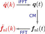
AFT is a versatile and computationally elegant technique for handling arbitrary nonlinear terms in CMs, which shifts the burden from the modeler to the computer.[74, 75, 76, 49] It provides a means to numerically compute $\hat{\bm{f}}_{\text{nl}}$ from $\hat{\bm{q}}$. Given a starting guess for the solution $\hat{\bm{q}}$, AFT involves three steps depicted schematically in Fig. 1:

1. $\hat{\bm{q}}(k)\rightarrow\bm{q}(t)$: Consider a dense time-domain grid of equispaced points $\{t_{j}\}_{j=1}^{N}\in[0,T]$. $N$ should be atleast twice the highest harmonic to avoid aliasing error; thus, $N\geq 2(2H+1)$. We take the vector of FCs $\hat{\bm{q}}$, and use inverse FFT (iFFT) to obtain $\bm{q}_{i}(\{t_{j}\})$ at these sample points for all the stress components ($1\leq i\leq 4$). The result of this frequency $\rightarrow$ time-domain step is a $4N$ dimensional vector $\bm{q}(\{t_{j}\})=[\bm{q}_{1}(\{t_{j}\}),\bm{q}_{2}(\{t_{j}\}),\bm{q}_{3}(\{t_{j}\}),\bm{q}_{4}(\{t_{j}\})]$ of time-domain stress samples.

2. $\bm{q}(t)\rightarrow\bm{f}_{\text{nl}}(t)$: Using the time-domain approximation $\bm{q}(\{t_{j}\})$, we compute the nonlinear term in the time domain by substituting $\bm{q}(t)$ in the expression for $\bm{f}_{\text{nl}}$ corresponding to the CM. The result of this step is a $4N$ dimensional vector of time-domain samples of the nonlinear terms $\bm{f}_{\text{nl}}(\{t_{j}\})$.

3. $\bm{f}_{\text{nl}}(t)\rightarrow\hat{\bm{f}}_{\text{nl}}$: Finally, we transform the time-domain samples of the nonlinear term $\bm{f}_{\text{nl}}(\{t_{j}\})$ back to the frequency domain $\hat{\bm{f}}_{\text{nl}}$ using FFT. We discard harmonics greater than $2H$ for the normal stresses and $2H+1$ for the shear stress to be consistent with the ansatz. It can be theoretically shown that AFT preserves the even and odd harmonics required by symmetry.

The $\hat{\bm{f}}_{\text{nl}}$ obtained using AFT is used in each iteration while solving the nonlinear equation system eqn. (23). Luckily, the computational cost of FFT and inverse FFT is $\mathcal{O}(N\log N)$. This is the cost that is shifted from the modeler to the computer.

Figure 1: Schematic of AFT scheme for evaluating $\hat{\bm{f}}_{\text{nl}}$ from $\hat{\bm{q}}$ using inverse FFT, the constitutive model (CM), and FFT. Frequency (time) domain quantities are shown in red (black).

III.1.3 Solving HB

We begin by choosing the number of harmonics $H$ in the ansatz. This choice is informed primarily by $\gamma_{0}$ and Wi. For small values of $\gamma_{0}$ or Wi, $H\approx 1-3$ is adequate. For larger values of $\gamma_{0}$ and Wi, larger values of $H$ may be required to resolve the LAOS response fully. In this work, we use $H=8$ as a standard for all computations unless otherwise specified. Note that this choice resolves shear stress up to the 17th harmonic!

Next, we select a good initial guess $\hat{\bm{q}}^{(0)}$ for the solution. If an analytical solution for the CM in SAOS or MAOS regime is available, then this is usually a good choice, especially for $\gamma_{0}\lesssim 1$. Otherwise, the UCM solution may be used as $\hat{\bm{q}}^{(0)}$ instead. In this work, we use the MAOS solution for the PTT model as the initial guess for $\gamma_{0}\leq 1$. For any $\gamma_{0}>1$ we create a ladder of strain amplitudes, where each subsequent rung of the ladder represents increasing $\gamma_{0}$. The first rung starts at $\gamma_{0}=1$, and uses the MAOS solution as $\hat{\bm{q}}^{(0)}$. The HB solution at each rung is then used as the initial guess for the next step. The spacing of $\gamma_{0}$ in the interval between 1 and the target strain amplitude is logarithmic with five rungs per decade. A similar laddered approach is also used for the TNM model. However, since the MAOS solution is not known, the first rung is taken to be $\gamma_{0}=10^{-2}$, and the UCM solution is used as the initial guess.

With this initial guess for $\hat{\bm{q}}^{(0)}$, we solve the system of nonlinear algebraic equations using the python interface (fsolve) to MINPACK’s hybrd method.[77, 78] The solver uses a modification of the hybrid Powell or dogleg method, in which the Jacobian is approximated by a forward-difference formula.[79] We use the default value for determining convergence: iteration is terminated when the relative error between consecutive iterates falls below $10^{-8}$.

III.2 Numerical Integration

Eqn. (16) specifies a periodic boundary value problem since the initial conditions $\bm{q}(0)$ are not explicitly specified. Instead, we seek a PSS solution for which,

$$\lim_{t\rightarrow\infty}\,q(t+T)=q(t).$$ (37)

One approach is to treat it as a boundary value problem and use the shooting method where we guess the initial condition $\bm{q}(0)$ and iteratively update it until the condition $\bm{q}(T)=\bm{q}(0)$ is met.[73] Each iteration of the shooting method involves solving the IVP for $t\in[0,T]$. A more conventional method of determining the alternance solution is to mimic the experimental setup and pose the ODE as an IVP with arbitrary initial conditions (e.g., $\bm{q}(0)=\bm{0}$). Fortunately, these initial conditions do not matter, and a PSS profile emerges after initial transients decay.

We use a 5th order implicit Runge-Kutta scheme of the Radau IIA family, implemented in the python package scipy with absolute and relative tolerances of $10^{-10}$ and $10^{-8}$, respectively.[80, 78] We use an implicit scheme because explicit schemes tend to struggle with high frequencies $\omega$ and strong nonlinearities. By default, we solve the problem for $t\in[0,n_{p}T]$ where $n_{p}=10$ is the number of periods.

For each period $p$, we consider the response over that period, $\bm{q}_{p}(s)$ where $s=t\text{ mod }T$, and ‘mod’ is the modulo or remainder operator. The response over the first period $\bm{q}_{1}(s)$ is typically nonperiodic because of the arbitrary choice of initial conditions. As $p$ increases, the $\bm{q}_{p}(s)$ approaches the alternance state. To quantify the approach to PSS, we evaluate $\bm{q}_{p}(s)$ over $N$ equispaced points $\{s_{i}\}_{i=1}^{N}\in[0,T]$. We compare the difference in $\bm{q}_{p}(s)$ over the last two of these periods ($n_{p}$ and $n_{p}-1$), by computing the metric,

$$E_{p}=\frac{1}{4N}\sqrt{\sum_{i=1}^{N}\left(\bm{q}_{n_{p}}(s_{i})-\bm{q}_{n_{p}-1}(s_{i})\right)^{2}}$$ (38)

If $E_{p}$ falls below the threshold $10^{-10}$, we take the solution obtained over the last period as $\bm{q}_{\text{NI}}\equiv\bm{q}_{n_{p}}$. Otherwise, we update initial conditions using the last cycle $\bm{q}_{n_{p}+1}(t=0)=\bm{q}_{n_{p}}(T)$ and repeat the calculation over $n_{p}$ more cycles until the threshold is met.

III.3 Quantifying Error

How can we determine the accuracy of numerical solutions when benchmark analytical solutions are not available? How can we compare the accuracy of the IVP and HB methods? One idea is to develop a time-domain error metric $\epsilon_{t}$ based on the residual corresponding to the IVP, $\bm{r}(\bm{q},\dot{\bm{q}},t)=\dot{\bm{q}}(t)+\bm{f}_{\text{nl}}(\bm{q},t)-\bm{f}_{\text{ex}}(t)$, and a frequency-domain error metric $\epsilon_{\omega}$ based on the residual corresponding to HB, $\hat{\bm{r}}^{H}(\hat{\bm{q}})\equiv\hat{\dot{\bm{q}}}+\hat{\bm{f}_{nl}}(\hat{\bm{q}})-\hat{\bm{f}}_{\text{ex}}$. If $\bm{q}(t)$ is an exact solution with FCs $\hat{\bm{q}}$, both the residuals $\bm{r}(\bm{q},\dot{\bm{q}},t)$ and $\hat{\bm{r}}^{H}(\hat{\bm{q}})$ would be identically zero. However, when $\bm{q}(t)$ is numerically approximated using the IVP or HB methods, the residuals are nonzero but hopefully small.

Let $\bm{q}_{\text{NI}}(t)$ and $\hat{\bm{q}}_{\text{HB}}$ be the solutions obtained using the IVP and HB methods for a given problem. We can interpolate $\bm{q}_{\text{NI}}(t)$ at a large number (say, $N=2^{6}$) of equispaced points $t_{i}\in[0,T]$, and take the FFT to obtain $\hat{\bm{q}}_{\text{NI}}$. To facilitate comparison, we only select even (odd) harmonics up to order $2H$ ($2H+1$) for normal (shear) stress. Typically, the harmonics that are not included are negligible. We can compute a frequency-domain error metric by directly substituting $\hat{\bm{q}}=\hat{\bm{q}}_{\text{NI}}$ or $\hat{\bm{q}}=\hat{\bm{q}}_{\text{HB}}$ into the expression for $\hat{\bm{r}}^{H}(\hat{\bm{q}})$. Since $\hat{\bm{r}}^{H}(\hat{\bm{q}})$ is a vector with $U$ elements, we set $\epsilon_{\omega}$ based on the root mean squared error (RMSE) of the residuals,

$$\epsilon_{\omega}(\hat{\bm{q}})=\dfrac{1}{\sqrt{U}}||\hat{\bm{r}}^{H}(\hat{\bm{q}})||_{2}.$$ (39)

To compute $\epsilon_{t}$, we use $\hat{\bm{q}}=\hat{\bm{q}}_{\text{NI}}$ or $\hat{\bm{q}}=\hat{\bm{q}}_{\text{HB}}$ and first estimate $\dot{\bm{q}}(t_{i})$ and $\bm{q}(t_{i})$ at $t_{i}\in[0,T]$, $1\leq i\leq N$, using eqn. (31). Again, we use the RMSE of the time-domain residuals as,

$$\epsilon_{t}(\bm{q})=\dfrac{1}{\sqrt{4N}}||\bm{r}(\bm{q})||_{2}.$$ (40)

Using this procedure, we can obtain $\epsilon_{t}$ and $\epsilon_{\omega}$ for both the NI and HB methods.

IV Results

IV.1 Validation of FLASH

We test the validity of FLASH by finding the LAOS response of the PTT model and the TNM at different operating conditions $(\gamma_{0},\omega)$. All calculations using FLASH or NI are performed with nondimensionalized equations. However, the solutions obtained are converted back to dimensional units when results are reported in this section and in supplementary material. We assume that the modulus $G=1$ Pa so that the moduli reported in figures 2 and 3 are expressed in units of $G$.

IV.1.1 Phan-Thien Tanner model

$\gamma_{0}=0.1$	$\gamma_{0}=10$
(a)	(b)
(c)	(d)

Figure 2: PTT model: The moduli corresponding to the first harmonic $G_{1}^{\prime}$ and $G_{1}^{\prime\prime}$ for (a) $\gamma_{0}=0.1$ and (b) $\gamma_{0}=10$, and the third harmonic $G_{3}^{\prime}$ and $G_{3}^{\prime\prime}$ for (c) $\gamma_{0}=0.1$ and (d) $\gamma_{0}=10$ obtained by NI and FLASH agree with each other. For $\gamma_{0}=0.1$, these solutions also agree with the analytical MAOS solution (AN).

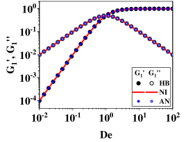
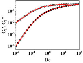
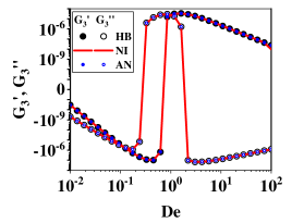
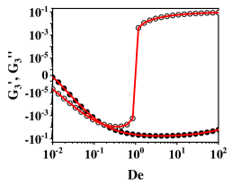
We set $\epsilon=0.1$ for this part. Fig. 2 depicts the shear response of the PTT model computed using FLASH at two different strain amplitudes in the MAOS $\left(\gamma_{0}=0.1\right)$ and LAOS $\left(\gamma_{0}=10\right)$ regimes. The first $(G_{1}^{\prime},G_{1}^{\prime\prime},)$ and third $(G_{3}^{\prime},G_{3}^{\prime\prime},)$ harmonics are plotted as a function of applied frequency. Fig. 2a and 2c show that the MAOS response obtained using FLASH agrees with the numerical solution of the IVP and the MAOS analytical solution (AN).[19] Similar agreement between FLASH and NI is observed in fig. 2b and 2d for the LAOS response. Additional plots of stress waveforms and the leading normal stress moduli are provided in the supplementary material.

IV.1.2 Temporary Network Model

Type I: Strain Softening	Type III: Weak Strain Overshoot
$a$ = -1.0, $b$ = 1.0	$a$ = 0.5, $b$ = 1.0
(a)	(b)
(c)	(d)

Figure 3: First and third harmonic moduli for the TNM with parameters chosen to illustrate type I (a and c), and type 3 (c and d) behavior at $\text{De}=5$ and different $\gamma_{0}$. The agreement between FLASH and NI is excellent.

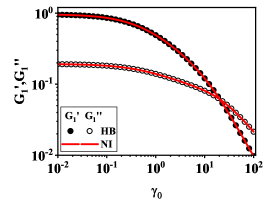
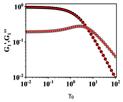
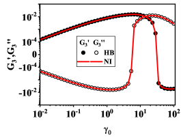
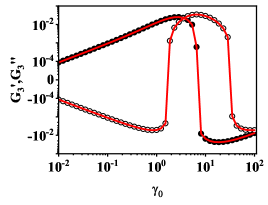
The Ahn-Osaki TNM captures four canonical types of LAOS behavior depending on the values of the parameters $a$ and $b$.[70, 16, 3] To validate FLASH, we illustrate two of these four categories, namely, type I or strain softening ($a$ = -1.0, $b$ = 1.0), and type III or weak strain overshoot ($a$ = 0.5, $b$ = 1.0). Figures 3a and 3b show the moduli associated with the first harmonic, while figures 3c and 3d show the moduli associated with the third harmonic. In type I behavior, $G_{1}^{\prime}$ and $G_{1}^{\prime\prime}$ decrease monotonically as $\gamma_{0}$ is increased, while in type III behavior, $G_{1}^{\prime\prime}$ exhibits a local maximum at intermediate $\gamma_{0}$. Calculations are performed at a fixed frequency corresponding to $\text{De}=5$ over four decades of $\gamma_{0}$. The agreement between FLASH and NI solutions is satisfactory. The non-differentiable absolute value function in the creation ($c(t)$) and destruction ($d(t)$) terms of the TNM introduces a first-order discontinuity and that presents some issues for FLASH, which we shall examine shortly. Nevertheless, these examples illustrate that FLASH is not only a flexible framework but also quite robust.

IV.2 Computational Cost

(a) Lissajous plots

(b) CPU

Figure 4: PTT model: (a) Normalized elastic Lissajous curves of the shear stress $\sigma_{12}$ vs $\gamma$, and (b) comparison of the computational time (in seconds) at three different values of $\gamma_{0}$ and De.

(a) Lissajous plots

(b) CPU

Figure 5: TNM - Type I: Normalized elastic Lissajous curves of the shear stress $\sigma_{12}$ vs $\gamma$, and (b) comparison of the computational time (in seconds) at three different values of $\gamma_{0}$ and De.

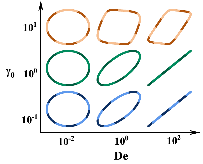
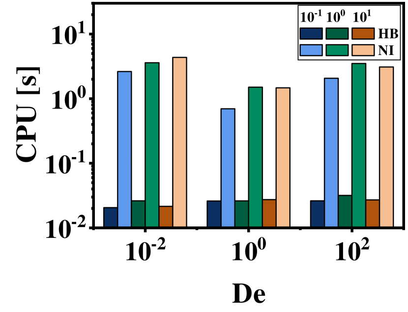
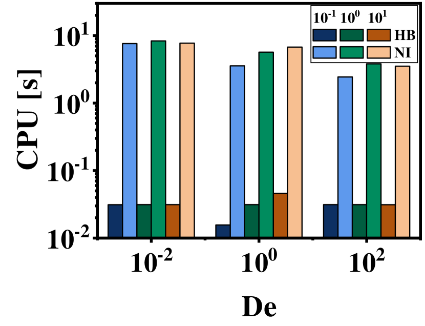
Figures 4(a) and 5(a) show a representative Pipkin diagram for the PTT model and type I case of the TNM model, respectively. These figures depict the elastic Lissajous curves for the shear stress, i.e. $\sigma_{12}(t)$ vs $\gamma(t)$, at three strain amplitudes $\left(10^{-1},10^{0},10^{1}\right)$ and three frequencies $\left(10^{-2},10^{0},10^{2}\right)$. Since the agreement between the two methods appears reasonable, we compare the CPU time required to compute these solutions in figures 4(b) and fig. 5(b) for the PTT model and the TNM, respectively. Calculations were performed on Intel i7-6700 3.4 GHz Windows workstation running Python 3.8.10, numpy 1.24.4, and scipy 1.10.1. On average, FLASH takes roughly 30 ms per evaluation for both CMs. NI takes longer: about 0.7 – 4.55 s for the PTT model and 2 – 8 s per evaluation for the TNM. Thus, it is evident that FLASH is between 1-3 orders of magnitude faster than NI, regardless of the operating condition. It is useful to note that even NI struggles with the first-order discontinuity in the TNM.

IV.3 Accuracy

(a) frequency domain error

(b) time domain error

Figure 6: The frequency and time domain error metrics for the HB (filled symbols) and NI (open symbols) methods. Calculations are performed at $\gamma_{0}=10$ for the PTT model (squares) and the type 1 TNM (triangles) with $H=8$.

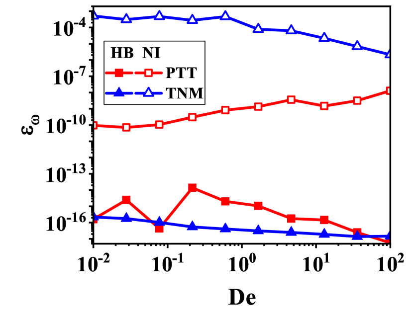
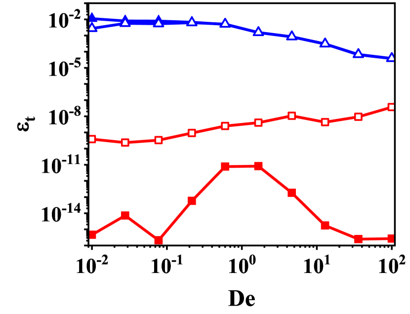
We compare the relative accuracy of the HB and IVP methods. Due to the absence of analytical solutions for nonlinear CMs, we examine accuracy using error metrics based on residuals in the time ($\epsilon_{t}$) and frequency domains ($\epsilon_{\omega}$) as described in section III.3. Figures 6(a) and 6(b) represent the frequency domain $\epsilon_{\omega}$ and time domain $\epsilon_{t}$ error metrics, respectively. Results for both the PTT model and the TNM are shown at a large strain amplitude of $\gamma_{0}=10$ over a range of frequencies. The parameters used for the TNM were $a=-1.0$ and $b=1.0$ corresponding to type I behavior, while $\epsilon=0.1$ was used for the PTT model.

From fig. 6(a), it is evident that FLASH is able to reach its desired target of minimizing the frequency space residual nearly to the level of machine precision. In terms of $\epsilon_{\omega}$, FLASH outperforms NI for both models, as expected. However, the accuracy of NI, as quantified by this metric, is also quite satisfactory. It is, therefore mildly surprising that in terms of $\epsilon_{t}$, FLASH leads to a lower error than NI for the PTT model, although the error is quite small for both methods. For the type I TNM in Fig. 6(b), the performance of both methods degrades to approximately the same level.

(a) PTT

(b) TNM

Figure 7: $\epsilon_{t}$ at different $H$ for the PTT and the TNM model at $\text{De}=1$ and different $\gamma_{0}=[10^{-1},10^{0},10^{1}]$.

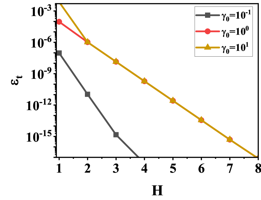
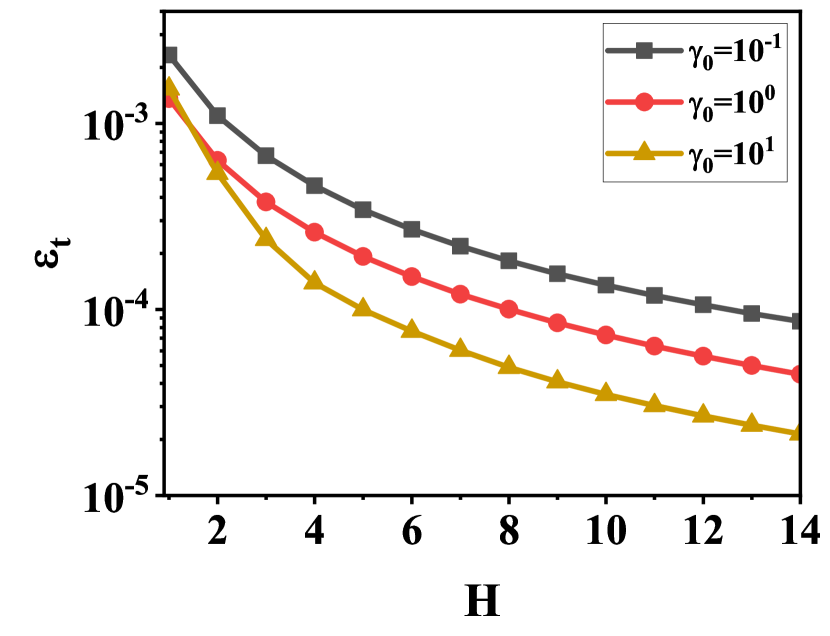
Two user-specified parameters in the FLASH algorithm affect accuracy: the number of data points $N$ in the AFT step and the number of harmonics $H$ in the ansatz. The choice of $N$ does not affect accuracy once it is large enough to avoid aliasing error, i.e. $N\geq 2(2H+1)$. Since the AFT scheme is based on the FFT, it is recommended to select $N$ as a power of two. A larger value of $N$ increases the computational cost asymptotically as $\mathcal{O}(N\log N)$.

The influence of $H$, on the other hand, is more interesting. For the PTT model, fig. 7(a) shows that $\epsilon_{t}$ decreases to machine precision as $H$ is increased to 8, even at large strain amplitudes. The linear and super-linear decay observed on the semilog plot indicates fast exponential convergence towards the true solution since the nonlinearity in the PTT model is analytic. In contrast, convergence is sluggish for the TNM. $\epsilon_{t}$ does not approach machine precision even for large $H$, as shown in fig. 7(b). Unsurprisingly, this loss of performance originates from the first-order discontinuity in the CM. Gibbs phenomenon is a well-known observation in which Fourier series representations struggle with sharp discontinuities. Such a Fourier series produces oscillations or “ringing artifacts” near the point of discontinuity, and the magnitude of the maximum overshoot cannot be reduced by simply increasing $H$. Thus, spectral convergence falters as $H$ is increased and the accuracy of the solution improves gradually. However, it is useful to emphasize that the creation and destruction terms used in this TNM are artificial; these terms are analytic in physically motivated TNMs and present no special issues for FLASH.

V Discussion

These results establish that FLASH is a fast and accurate method. We discuss how it can be conveniently generalized to other nonlinear CMs, and the potential applications that are unlocked by these attributes.

V.1 General nonlinear differential constitutive equations

To adapt FLASH to any arbitrary nonlinear CM, we only need to adapt the nonlinear term $\bm{f}_{\text{nl}}$ corresponding to the CM in eqn. (16). Thus far, we already presented $\bm{f}_{\text{nl}}$ for the UCM, PTT, and TNM models by eqns. (26), (27) and (28), respectively. Here, we offer $\bm{f}_{\text{nl}}$ for some commonly encountered differential CMs. Additional CMs are entertained in supplementary material.

For clarity, we revert to the dimensional form of CMs in this section. Although non-dimensionalization is recommended for both FLASH and NI as it partially mitigates numerical difficulties encountered at high Wi, it is not a pre-condition for numerical computation. Let us define the unknown variables as $\bm{q}=[\sigma_{11},\sigma_{22},\sigma_{33},\sigma_{12}]$, and the external forcing term $\bm{f}_{\text{ex}}=G\dot{\gamma}\bm{e}_{4}$ in dimensional form. For OS flow, we can usually drop $\sigma_{33}$ and all terms associated with it in $\bm{f}_{\text{nl}}$ and $\bm{f}_{\text{ex}}$.

Consider the Oldroyd 8-constant linear CM,[28]

$$\bm{\sigma}+\lambda_{1}\stackrel{{\scriptstyle\triangledown}}{{\bm{\sigma}}}+\frac{1}{2}\lambda_{3}\left(\bm{\gamma}_{(1)}\cdot\bm{\sigma}+\bm{\sigma}\cdot\bm{\gamma}_{(1)}\right)+\frac{1}{2}\lambda_{5}\left(\text{tr}(\bm{\sigma})\right)\bm{\gamma}_{(1)}+\frac{1}{2}\lambda_{6}\left(\bm{\sigma}:\bm{\gamma}_{(1)}\right)\bm{\delta}$$

$$-G\left(\bm{\gamma}_{(1)}+\lambda_{2}\bm{\gamma}_{(2)}+\lambda_{4}\left(\bm{\gamma}_{(1)}\cdot\bm{\gamma}_{(1)}\right)+\frac{1}{2}\lambda_{7}\left(\bm{\gamma}_{(1)}:\bm{\gamma}_{(1)}\right)\bm{\delta}\right)=\bm{0}$$ (41)

where the derivatives of strain, indicated by subscripts in parenthesis, are given by,

$$\bm{\gamma}_{(1)} =\dot{\gamma}\bm{e}_{1}\bm{e}_{2}+\dot{\gamma}\bm{e}_{2}\bm{e}_{1}$$

$$\bm{\gamma}_{(2)} =-2\dot{\gamma}^{2}\bm{e}_{1}\bm{e}_{1}+\ddot{\gamma}\bm{e}_{1}\bm{e}_{2}+\ddot{\gamma}\bm{e}_{2}\bm{e}_{1}$$

for OS flow. Here, $\ddot{\gamma}=d\dot{\gamma}/dt$. The $\{\lambda_{i}\}_{i=1}^{7}$ and $G$ constitute the 8 model parameters, lending the model its name. Many popular CMs are special cases of this model. A short list is shown in Table 1; more exhaustive lists are available elsewhere.[81, 28]

For OS flow, the nonlinear term needed by FLASH is found to be,

$$\bm{f}_{\text{nl}}^{\textbf{OD8}} =\left(\frac{\sigma_{11}}{\lambda_{1}}-\dot{\gamma}\sigma_{12}\left(2-\frac{\lambda_{3}}{\lambda_{1}}-\frac{\lambda_{6}}{\lambda_{1}}\right)-\frac{1}{2}\frac{\lambda_{6}}{\lambda_{1}}\dot{\gamma}\left(\sigma_{11}+\sigma_{22}\right)+G\dot{\gamma}^{2}\left(2\lambda_{2}-\lambda_{4}-\frac{1}{2}\lambda_{7}\right)\right)\text{ }\bm{e}_{1}$$

$$+\left(\frac{\sigma_{22}}{\lambda_{1}}-\dot{\gamma}\sigma_{12}\left(\frac{\lambda_{3}}{\lambda_{1}}+\frac{\lambda_{6}}{\lambda_{1}}\right)-\frac{1}{2}\frac{\lambda_{6}}{\lambda_{1}}\dot{\gamma}\left(\sigma_{11}+\sigma_{22}\right)-G\dot{\gamma}^{2}\left(\lambda_{4}+\frac{1}{2}\lambda_{7}\right)\right)\text{ }\bm{e}_{2}$$

$$+\left(\frac{\sigma_{33}}{\lambda_{1}}+\frac{1}{2}\frac{\lambda_{6}}{\lambda_{1}}\dot{\gamma}\left(\sigma_{11}+\sigma_{22}+2\sigma_{12}\right)-\frac{1}{2}G\lambda_{7}\dot{\gamma}^{2}\right)\text{ }\bm{e}_{3}$$

$$+\left(\frac{\sigma_{12}}{\lambda_{1}}+\dot{\gamma}\sigma_{11}\left(\frac{\lambda_{3}+\lambda_{5}}{2\lambda_{1}}\right)+\dot{\gamma}\sigma_{22}\left(\frac{\lambda_{3}+\lambda_{5}-2\lambda_{1}}{2\lambda_{1}}\right)-G\lambda_{2}\frac{d\dot{\gamma}}{dt}\right)\text{ }\bm{e}_{4}.$$ (42)

With this information, ideally coupled with nondimensionalization, it is straightforward to determine the LAOS response of the Oldroyd 8-constant model and its special cases using FLASH. Interestingly, for CMs that are linear in $\bm{\sigma}$ such as the Oldroyd 8-constant model, it is possible to develop a specialized HB method that does not require AFT to calculate $\hat{\bm{f}}_{\text{nl}}$. Although this approach requires additional manual effort for setup, it handily outperforms even analytical solutions, as recently reported for the corotational Maxwell model.[50]

Constitutive Model	Special Case
Upper Convected Maxwell	$\lambda_{2}=\lambda_{3}=\lambda_{4}=\lambda_{5}=\lambda_{6}=\lambda_{7}=0$
Oldroyd A fluid	$\lambda_{3}=2\lambda_{1},\lambda_{4}=2\lambda_{2},\lambda_{5}=\lambda_{6}=\lambda_{7}=0$
Oldroyd B fluid (convected Jeffreys)	$\lambda_{3}=\lambda_{4}=\lambda_{5}=\lambda_{6}=\lambda_{7}=0$
Corotational Jeffreys Model	$\lambda_{3}=\lambda_{1},\lambda_{4}=\lambda_{2},\lambda_{5}=\lambda_{6}=\lambda_{7}=0$
Johnson-Segalman model${}^{\text{a}}$	$\lambda_{1}=\frac{\eta_{s}\lambda}{\eta_{0}},\lambda_{2}=\zeta_{\text{JS}}\lambda,\lambda_{3}=\frac{\zeta_{\text{JS}}\eta_{s}\lambda}{\eta_{0}}$
	$\lambda_{4}=\lambda_{5}=\lambda_{6}=\lambda_{7}=0$

Table 1: Selected special cases of the Oldroyd 8 constant model. ${}^{\text{a}}$ For the Johnson-Segalman model, $G=\eta_{0}^{2}/(\lambda\eta_{s})$ and $\eta_{0}=\eta_{s}+\eta_{p}$, where $\eta_{s}$ and $\eta_{p}$ represent the solvent and polymer viscosity contributions. $\lambda$ is the relaxation time and $\zeta_{\text{JS}}$ is an additional model parameter.

Analogous to the Oldroyd 8-constant model, the generalized Maxwell-like CM presented by Song et al.[19] has several nonlinear CMs for polymer melts and solutions as special cases. It reduces to the UCM model in the linear limit. For uniformity, we use the stress tensor $\bm{\sigma}$ in our exposition instead of the conformation tensor used by the authors. This CM is then given by

$$\stackrel{{\scriptstyle\triangledown}}{{\bm{\sigma}}}+\zeta\left(\bm{\gamma}_{(1)}\cdot\bm{\sigma}+\bm{\sigma}\cdot\bm{\gamma}_{(1)}\right)+\frac{1}{\lambda}\bm{H}(\bm{\sigma})+\bm{J}(\bm{\sigma})-(1-\zeta)G\bm{\gamma}_{(1)}=\bm{0}$$ (43)

where $G$ and $\lambda$ are linear viscoelastic parameters, $0<\zeta<1$, and different expressions for $\bm{H}(\bm{\sigma})$ and $\bm{J}(\bm{\sigma})$ correspond to different popular nonlinear CMs (see Table 2 for some examples). In OS flow, the nonlinear term required by FLASH is

$$\bm{f}_{\text{nl}}^{\textbf{GM}} =\left(2\zeta\sigma_{12}\dot{\gamma}+\frac{1}{\lambda}H_{11}(\bm{\sigma})+J_{11}(\bm{\sigma})\right)\text{ }\bm{e}_{1}+\left(2\zeta\sigma_{12}\dot{\gamma}+\frac{1}{\lambda}H_{22}(\bm{\sigma})+J_{22}(\bm{\sigma})\right)\text{ }\bm{e}_{2}$$

$$+\left(\frac{1}{\lambda}H_{33}(\bm{\sigma})+J_{33}(\bm{\sigma})\right)\text{ }\bm{e}_{3}+\left(\zeta\dot{\gamma}\left(\sigma_{11}+\sigma_{22}\right)+\frac{1}{\lambda}H_{12}(\bm{\sigma})+J_{12}(\bm{\sigma})+G\zeta\dot{\gamma}\right)\text{ }\bm{e}_{4}.$$ (44)

Constitutive Equation	Special Case
Giesekus Modela	$\zeta=0,\bm{J}(\bm{\sigma})=0$, $\bm{H}(\bm{\sigma})=\bm{\sigma}+\frac{\alpha}{G}\bm{\sigma\cdot\sigma}$
Phan Thien Tanner Modelb	$\zeta\neq 0,\bm{J}(\bm{\sigma})=0,\bm{H}(\bm{\sigma})=Y(\text{tr }\bm{\sigma})\bm{\sigma}$
Rolie-Poly modelc	$\zeta=0,\bm{H}(\bm{\sigma})=\bm{\sigma},\bm{J}(\bm{\sigma})\neq 0$

Table 2: Some commonly used nonlinear differential CMs. ^a For the Giesekus model this assumes solvent viscosity $\eta_{s}=0$. ^b For the PTT model $Y(\text{tr }\bm{\sigma})=1+\epsilon\left(\text{tr }\bm{\sigma}\right)$ or $Y(\text{tr }\bm{\sigma})=\exp{\left(\text{tr }\bm{\sigma}\right)}$ are commonly used forms.[19] ^c For the Rolie-Poly model $\bm{J}(\bm{\sigma})$ takes different forms based on the character of chains.[19]

Several nonlinear CMs, such as the pom-pom model, do not fit the mold of equation (43). In such cases, we track additional dynamical variables by supplementing the $\bm{q}$ vector, as demonstrated in supplementary material.

V.2 Model calibration and model selection

As mentioned in section I.1, one way to digest and interpret LAOS data is to first assimilate it into a suitable CM by fitting the model parameters. This step is called model calibration. Examples of model calibration based on OS data include studies of colloidal gels,[82, 83] wormlike micellar solutions,[22, 84] cross-linked hydrogel systems,[21, 85] polymer melts and solutions,[2, 86, 87, 88] etc. Typically, SAOS data are fitted first to obtain linear viscoelastic parameters. For real systems, this may entail extraction of discrete or continuous relaxation spectra using software like DISCRETE, IRIS, or pyReSpect.[89, 90, 91, 92, 93]

Subsequently, LAOS data is used to determine the nonlinear model parameters.[94] Model calibration requires multiple evaluations of the CM with different parameter choices to determine the best fit. The number of model evaluations required can range between $\mathcal{O}(10^{3})-\mathcal{O}(10^{5})$ depending on the number of $\gamma_{0}$ and $\omega$ explored, required accuracy, and desire for uncertainty quantification. In such cases, the speed and accuracy advantage of FLASH over NI can practically mean the difference between an hour or several days of computation.

For many materials, such as polymers, multiple CMs may serve as equally attractive candidates at the outset. The goal of model selection is to select the best of these potential candidates, perhaps for inclusion in computational fluid dynamics software. Model selection seeks to balance goodness-of-fit and model complexity to avoid over-fitting. Simple techniques for model selection include the Akaike or Bayesian information criteria, which penalize models with many parameters. Furthermore, a well-chosen CM aids both scientific discovery (statistical inference) and prediction (statistical prediction). For example, Suman et al. used the functional dependence of damping factor on shear rate obtained from steady shear experiments to predict the LAOS behavior of a critical gel system and make inferences about the change in material microstructure.[82] This study used a spectral method for integral CMs to expedite the process.[95] FLASH brings the same power to differential CMs, which are far more plentiful than integral CMs.

V.3 Thermodynamic Studies

The speed and accuracy of FLASH not only aid in the interpretation of experimental LAOS data but also enable theoretical studies that have only been performed rarely due to the associated computational cost. One such application is marking the region of thermodynamic stability of CMs in LAOS flow. For demonstration, we employ the Ziegler criterion, which is rooted in nonequilibrium thermodynamics, as formulated by Saengow and Giacomin to study the corotational Maxwell model.[81] The objective here is only to provide a glimpse of the potential that FLASH unleashes, without necessarily commenting on whether it is the best way to study stability.

Saengow and Giacomin [81] observed that polymeric liquids subjected to large oscillatory deformations tend to become aperiodic due to the formation of new thermodynamic phases. According to the Ziegler criterion (simplified version of eqn. 83 in their paper), thermodynamic instability is encountered when

$$Z=-\gamma_{0}\left.\frac{\partial G_{1}^{\prime\prime}}{\partial\gamma_{0}}\right|_{\text{De}}-G_{1}^{\prime\prime}\geq 0,$$ (45)

where $G_{1}^{\prime\prime}$ is primary loss modulus in equations (1) and (5). Note that eqn. (45) can be further simplified as,

$$\left.\frac{\partial\log{G_{1}^{\prime\prime}}}{\partial\log{\gamma_{0}}}\right|_{\text{De}}\leq-1,$$ (46)

which links thermodynamic instability to extreme strain-softening.

In order to make phase diagrams of thermodynamic stability, the CM has to be evaluated on a dense grid in Pipkin space ($\gamma_{0}$ versus $\omega$). The ladder-based approach for generating initial guesses in FLASH is well-suited for systematically exploring Pipkin space. The PSS solution at a particular value of $\gamma_{0}$ automatically serves as an excellent initial guess for the solution at a slightly higher value of $\gamma_{0}$. Besides improving the precision of the boundary between stable and unstable phases, a dense $\gamma_{0}$ grid is also required to evaluate the gradient $\partial G_{1}^{\prime\prime}/\partial\gamma_{0}$. However, for smooth curves such $\log{G_{1}^{\prime\prime}}$ versus $\log{\gamma_{0}}$, it is reasonable to obtain $G_{1}^{\prime\prime}$ for some specific values of $\gamma_{0}$ using FLASH and interpolate the rest of the data to obtain a dense grid for calculating the gradient. Nevertheless, creating contour maps of $Z$ using eqn (45) can become computationally expensive and has thus far been restricted to CMs with analytical OS solutions such as the corotational Maxwell model. FLASH frees us from this constraint.

PTT Model

(a) $\epsilon=0.1$, CPU $\approx$ 93s

Giesekus Model

(b) $\alpha=0.5$, CPU $\approx$ 96s

(c) $\text{De}=1$, CPU $\approx$ 62 s

(d) $\text{De}=1$ CPU $\approx$ 66 s

Figure 8: Contour plots of $Z$ for the PTT (left column) and Giesekus (right column) models. The top row spans a range of frequencies, holding the nonlinear model parameter ($\epsilon$ or $\alpha$) fixed. The bottom row spans a range of values for the model parameters at a particular frequency. The thick black lines in (b) and (d) correspond to $Z=0$ and mark the boundary of stability using the Ziegler criterion.

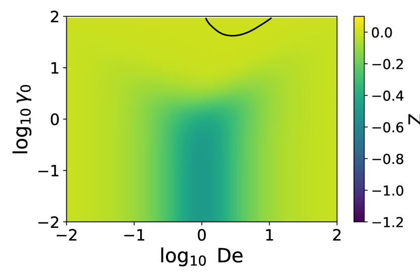
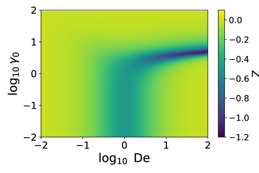
Figures 8(a) and 8(b) show contour maps based on the Ziegler criteria for the PTT model $(\epsilon=0.1)$ and the Giesekus model $(\alpha=0.5)$ respectively. We use the Giesekus model in lieu of the TNM because it is a single parameter model, which allows us to visualize the phase diagram more easily. In order to generate these plots, $G_{1}^{\prime\prime}$ is obtained on a logarithmically equispaced grid of De and $\gamma_{0}$. We use 65 different value of $\text{De}\in[10^{-2},10^{2}]$, and 80 different values of $\gamma_{0}\in[10^{-2},10^{2}]$.

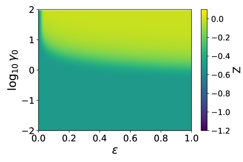
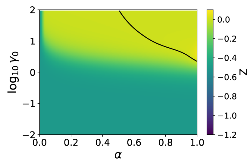
For $\text{Wi}<1$, a small number of harmonics $(H=3)$ is sufficient to obtain an accurate solution, while $H=6$ was used when $\text{Wi}\geq 1$. In accordance with $H$, $N=2^{5}$ was used for all the computations. Subsequently, the data are interpolated using cubic splines, from which the gradient $d\log{G_{1}^{\prime\prime}}/d\log{\gamma_{0}}$ is analytically computed. A similar approach was used to obtain Figures 8(c) and 8(d), where the model parameters for the PTT and the Giesekus models were varied, keeping the frequency fixed ($\text{De}=1$). Plots analogous to figure 8 for the CMM and the TNM are provided in the supplementary information.

It is evident from 8(a) and 8(c) that the PTT model is stable across the entire range of strains, frequencies, and model parameters probed. On the other hand, figure 8(b) indicates that the Giesekus model tends to become thermodynamically unstable in the large $\gamma_{0}$ regime $(\gamma_{0}>10)$. This is an expected outcome since the model shows a strong strain softening in this regime. Furthermore, figure 8(d) shows that this transition from stable to unstable region happens at a lower $\gamma_{0}$ as the model parameter is increased. This is likely a consequence of the increasing importance of the quadratic nonlinear term. The CPU time required for generating each of the top two figures was about 1.5 min, where FLASH was evaluated nearly $5000$ (65 $\times$ 80) times. The bottom two plots required about 1.25 min, for a similar number of model evaluations. It is worthwhile to point out that similar thermodynamic stability plots for the corotational Maxwell model on a coarser $(\gamma_{0},\omega)$ mesh took about 12 - 24h using NI.[81]

V.4 Stable and Unstable Solutions

Figure 9: (a) LAOS shear stress response of the Giesekus model $(\alpha=0.1)$ at $\gamma_{0}=10$ and $\text{De}=10$ obtained by using (i) the UCM solution, and (ii) the MAOS solution as initial guess values to FLASH, and (iii) NI. (b) the time and frequency domain error metrics for the three solutions.

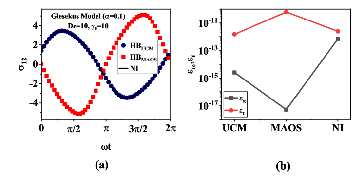
Nonlinear CMs, like other nonlinear dynamical systems, can exhibit multiple solutions when subjected to large perturbations. Some of these solutions may be stable, while others may be unstable. Depending on the initial condition, a dynamical system follows a unique trajectory to reach a time-invariant state called the attractor. Each attractor has its basin of attraction, i.e., the set of initial conditions that lead to that solution. Depending on the nature of the attractor, the asymptotic trajectory can be classified as fixed point, periodic oscillation, quasi-periodic, or chaotic.[49] If an asymptotic solution is mathematically unstable, we do not expect to observe it in experiments or even in NI solutions due to environmental or numerical perturbations. Nevertheless, it is essential to study the stability characteristics of dynamical systems because, in addition to theoretical insights, they provide robust limits that are directly relevant to computational fluid dynamics calculations.

Unlike thermodynamic stability analysis, which can also be carried out using NI, albeit at a significant computational cost, only HB allows us to track stable and unstable solution branches. Since HB solves nonlinear algebraic equations that have multiple solutions, we can potentially describe all possible solutions simply by tweaking the initial guess.

We illustrate this capability in figure 9a. Here, the LAOS solution of the Giesekus model $(\alpha=0.1)$ at $\gamma_{0}=10$ and $\text{De}=10$ is obtained using FLASH for two different initial guesses: (i) the UCM model solution, and (ii) the MAOS solution. We also present the ‘stable’ solution obtained using NI, which visually overlaps with the HB solution that uses the UCM response as the initial guess. This suggests that the HB solution using the MAOS response as the initial guess is unstable. To confirm that both the solutions obtained using FLASH are valid, we show the error metrics based on the frequency and time domain residuals in Fig. 9b. The low values of these error metrics ($\lesssim 10^{-10}$) indicates that all three solutions plotted in Fig. 9a are reasonable.

A PSS solution is said to be asymptotically stable if all the trajectories that start in its vicinity remain there. A standard procedure for asymptotic stability analysis involves computing the eigenvalues of a monodromy matrix and using the Floquet theorem to assess the stability.[96, 97] An alternative frequency domain method, that is more compatible with HB, is Hill’s method.[98, 99] Bifurcations, where the stability of a periodic solution changes character in response to changes in model parameters or operating conditions, can also be studied with HB.[49] Hill’s method can be combined with numerical path continuation to generate phase diagrams for mathematical stability.

VI Summary and Conclusions

HB is a Fourier-Galerkin method that transforms a system of nonlinear ODEs defined by the CM to a system of nonlinear algebraic equations. However, this transformation cannot be performed analytically for all nonlinear CMs. AFT is a numerical scheme that overcomes this obstacle by numerically shuttling between time and frequency domains. This work presents FLASH, a flexible method and computer program that combines HB with the AFT scheme to compute the PSS LAOS response of arbitrary nonlinear differential CMs. This offers a convenient interface for adapting HB to arbitrary CMs by shifting the burden of setting up equations in the right format from the modeler to the computer.

FLASH is validated using two CMs: the exponential PTT model, and a variant of the TNM. Its speed and accuracy is compared with the standard method of solving IVPs using NI. For the PTT model, FLASH is several orders of magnitude more accurate while also being 1-2 orders of magnitude faster. For the TNM, the superiority of FLASH over NI is less pronounced. In terms of the time-domain residual, they both perform equally well, while FLASH outperforms NI by several orders of magnitude in terms of the frequency-domain residual. FLASH retains its speed advantage for the TNM. As the number of harmonics $H$ in the ansatz increases, it shows exponential convergence for the PTT model, which degrades for the TNM due to a first-order discontinuity in the CM.

The speed and accuracy of FLASH open new avenues for theoretical studies of CMs, such as thermodynamic stability and the presence of stable and unstable solution branches. Combined with the spectral method [95] for integral CMs, FLASH offers a compelling toolbox for interpreting LAOS data through the lens of a CM and for model calibration and selection.

VII Appendix

VII.1 Fourier Series

Any periodic function $f(t)$ with period $T$, $f(t+T)=f(t)$, can be approximated by a truncated Fourier series. It can be represented using either complex exponential or trigonometric basis functions. In this work, we choose the latter because it facilitates numerical computation by relying only on “real” algebra. Thus,

$$f(t)\approx f^{H}(t)=\hat{f}(0)+\sum_{k=1}^{H}\hat{f}_{c}(k)\cos k\omega t+\hat{f}_{s}(k)\sin k\omega t,$$ (47)

where $H$ determines the order of truncation. The $2H+1$ trigonometric basis functions $\bm{B}_{H}(t)=[1,\cos\omega t,\cos 2\omega t,\cdots,\cos H\omega t,\sin\omega t,\sin 2\omega t\cdots,\sin H\omega t]$. The Fourier coefficients (FCs), for $k=0,1,\cdots,H$, are given by

$$\hat{f}(0) =\frac{1}{T}\int_{0}f(t)\,dt$$

$$\hat{f}_{c}(k) =\frac{2}{T}\int_{0}\cos(k\omega t)\cdot f(t)\,dt$$

$$\hat{f}_{s}(k) =\frac{2}{T}\int_{0}\sin(k\omega t)\cdot f(t)\,dt.$$ (48)

Following the order of the basis functions in $\bm{B}_{H}(t)$, we can arrange these FCs into a $2H+1$-dimensional vector $\hat{\bm{f}}=[\hat{f}(0),\hat{f}_{c}(1),\hat{f}_{c}(2),\cdots,\hat{f}_{c}(H),\hat{f}_{s}(1),\hat{f}_{s}(2),\cdots,\hat{f}_{s}(H)]$. Thus, the dot product $\hat{\bm{f}}\cdot\bm{B}_{H}(t)=f^{H}(t)$ expresses a linear combination of the basis functions determined by the FCs. This allows us to approximate and encode a continuous periodic time-domain function $f(t)$ as a discrete frequency domain representation $\hat{\bm{f}}$. This is attractive for the following reasons:

• Spectral accuracy: If the function $f(t)$ is analytic (infinitely differentiable), the FCs decay at an exponential rate, i.e $|\hat{f}_{c}(k)|$ and $|\hat{f}_{s}(k)|\leq Fc^{-k}$, where $c>1$ and $F$ is positive. Practically, this means that we can accurately approximate $f(t)$ with a relatively small number of harmonics $H$.

• Computational Efficiency: $\hat{\bm{f}}$ can be calculated efficiently from $N$ discrete equispaced samples of $f(t)$ in the domain $[0,T)$ using fast Fourier transform (FFT) at a cost of $\mathcal{O}(N\log N)$. If $N$ is too small, improper resolution of high-frequency components of $f(t)$ results in distortion of low-frequency components, a problem known as aliasing. This can be prevented by choosing $N\geq 2H+1$.

• Orthogonality of Basis Functions: Let $B_{H,i}(t)$ and $B_{H,j}(t)$ be any two basis functions from the set $\bm{B}_{H}(t)$, where the subscripts $i$ and $j$ correspond to their positions in the set. Then, their inner product is given by,

  $$\langle B_{H,i}\,B_{H,j}\rangle=\frac{2}{T}\int_{0}B_{H,i}(t)\,B_{H,j}(t)\,dt=\begin{cases}2&i=j=1\\ \delta_{ij}&\text{otherwise}.\end{cases}$$ (49)

  This relation allows us to conveniently pose the system of differential equations in weak form using a weighted residual method.

• Differential equations become algebraic equations: The derivative of the periodic function $\dot{f}^{H}(t)=df^{H}(t)/dt$ is (see eqn. 47),

  $$\hat{\dot{f}}^{H}(t) =\sum_{k=1}^{H}(k\omega)\hat{f}_{c}(k)(-\sin k\omega t)+(k\omega)\hat{f}_{s}(k)\cos k\omega t$$

  $$=\sum_{k=1}^{H}\left[(k\omega)\,\hat{f}_{s}(k)\,\cos k\omega t+(-k\omega)\,\hat{f}_{c}(k)\,\sin k\omega t\right].$$

  Thus, the Fourier representation $\hat{\dot{\bm{f}}}$ of $\dot{f}^{H}(t)$ can easily be obtained in terms of the FCs $\hat{\bm{f}}$ as, $\hat{\dot{\bm{f}}}=[0,\omega\hat{f}_{s}(1),\cdots,H\omega\hat{f}_{s}(H),-\omega\hat{f}_{c}(1),\cdots,-H\omega\hat{f}_{c}(H)]$. This allows us to transform the problem from solving nonlinear ODEs for $f(t)$ in the time domain to solving algebraic equations for $\hat{\bm{f}}$ in the frequency domain.

VII.2 HB equations for UCM model

The system of ODEs for the Upper Convected Maxwell model subjected to oscillatory shear strain deformation can be given by:

$$\dot{\sigma}_{11} +\frac{1}{\lambda}\sigma_{11}-2\dot{\gamma}\sigma_{12}=0$$

$$\dot{\sigma}_{22} +\frac{1}{\lambda}\sigma_{22}=0$$

$$\dot{\sigma}_{33} +\frac{1}{\lambda}\sigma_{33}=0.$$

$$\dot{\sigma}_{12} +\frac{1}{\lambda}\sigma_{12}-\dot{\gamma}\sigma_{22}=G\dot{\gamma}$$ (50)

Due to linearity, these equations can be solved analytically. Equations for $\sigma_{22}$ and $\sigma_{33}$ are decoupled from $\sigma_{11}$ and $\sigma_{12}$, and can be solved independently. At sufficiently long times, both these components decay to zero as $\sigma_{22}(t)/\sigma_{22}(0)=\sigma_{33}(t)/\sigma_{33}(0)=e^{-t/\lambda}$. Since $\sigma_{22}(t\rightarrow\infty)=0$, the equation for the shear stress $\sigma_{12}(t)$ also decouples and has the classic solution given by eqn.(3) similar to the linear Maxwell model. The PSS for the first normal stress difference, on the other hand, takes the form of eqn. (4), where $F_{0}^{\prime\prime}=G^{\prime}(\omega)$, $F_{2}^{\prime}=-G^{\prime}(\omega)+\frac{1}{2}G^{\prime}(2\omega)$ and $F_{2}^{\prime\prime}=G^{\prime\prime}(\omega)-\frac{1}{2}G^{\prime\prime}(2\omega)$

The Fourier transform $\hat{\bm{f}}_{\text{nl}}=\left[\hat{\bm{f}}_{\text{nl},1},\hat{\bm{f}}_{\text{nl},2},\hat{\bm{f}}_{\text{nl},3},\hat{\bm{f}}_{\text{nl},4}\right]$ of the nonlinear term $\bm{f}_{\text{nl}}$ given by eqn. 26 can be determined analytically. The first component is given by

$$\hat{\bm{f}}_{\text{nl},1}^{\text{UCM}} =\left(\hat{q}_{1}(0)-\text{Wi}\hat{q}_{c,4}(1)\right)\bm{e}_{1}+\sum_{k=1}^{H}\hat{q}_{c,1}(2k)-\text{Wi}\left(\hat{q}_{c,4}(2k-1)+\hat{q}_{c,4}(2k+1)\right)\text{ }\bm{e}_{k+1}$$ (51)

$$+\sum_{k=1}^{H}\hat{q}_{s,1}(2k)-\text{Wi}\left(\hat{q}_{s,4}(2k-1)+\hat{q}_{s,4}(2k+1)\right)\text{ }\bm{e}_{k+H+1}.$$ (52)

For $i=$ 2 and 3,

$$\hat{\bm{f}}_{\text{nl},i}^{\text{UCM}}=\hat{q}_{i}(0)\text{ }\bm{e}_{1}+\sum_{k=1}^{H}\hat{q}_{c,i}(2k)\text{ }\bm{e}_{k+1}+\hat{q}_{s,i}(2k)\text{ }\bm{e}_{k+H+1}.$$ (53)

Finally the term corresponding to the shear stress

$$\hat{\bm{f}}_{\text{nl},4}^{\text{UCM}} =\sum_{k=0}^{H}\hat{q}_{c,4}(2k+1)-\frac{\text{Wi}}{2}\left(\hat{q}_{c,2}(2k)+\hat{q}_{c,2}(2k+2)\right)\text{ }\bm{e}_{k+1}$$ (54)

$$+\sum_{k=0}^{H}\hat{q}_{s,4}(2k+1)-\frac{\text{Wi}}{2}\left(\hat{q}_{s,2}(2k)+\hat{q}_{s,2}(2k+2)\right)\text{ }\bm{e}_{k+H+2}.$$ (55)

We formulate the HB equation system by using eqns. (34) – (35) and (52) – (55) to obtain equations of the form eqn. (23).

$$\hat{r}_{c,1}(2k)=2k\text{De}q_{s,1}(2k)+q_{c,1}(2k)-\text{Wi}\left(q_{c,4}(2k-1)+q_{c,4}(2k+1)\right)$$ (56)

$$\hat{r}_{s,1}(2k)=-2k\text{De}q_{c,1}(2k)+q_{s,1}(2k)-\text{Wi}\left(q_{s,4}(2k-1)+q_{c,4}(2k+1)\right)$$ (57)

$$\hat{r}_{c,2}(2k)=2k\text{De}q_{s,2}(2k)+q_{c,2}(2k)$$ (58)

$$\hat{r}_{s,2}(2k)=-2k\text{De}q_{c,2}(2k)+q_{s,2}(2k)$$ (59)

$$\hat{r}_{c,3}(2k)=2k\text{De}q_{s,3}(2k)+q_{c,3}(2k)$$ (60)

$$\hat{r}_{s,3}(2k)=-2k\text{De}q_{c,3}(2k)+q_{s,3}(2k)$$ (61)

for the ODEs describing the evolution of the normal stresses with $k\in(1,H)$, and

$$\hat{r}_{c,4}(2k+1)=(2k+1)\text{De}q_{s,4}(2k+1)+q_{c,4}(2k+1)-\frac{\text{Wi}}{2}\left(q_{c,2}(2k)+q_{c,2}(2k+2)\right)-\delta_{k,0}$$ (62)

$$\hat{r}_{s,4}(2k+1)=-(2k+1)\text{De}q_{c,4}(2k+1)+q_{s,4}(2k+1)-\frac{\text{Wi}}{2}\left(q_{s,2}(2k)+q_{s,2}(2k+2)\right)$$ (63)

for fourth ODE corresponding to $\sigma_{12}$ with $k\in(0,H)$. From inspection, we find that all these equations are identically zero except for the case of $k=0$ and $k=1$ in eqn. (57), $k=1$ in eqn. (58), and $k=0$ in eqns. (62) and (63). This set of five equations can be solved analytically. Unsurprisingly, they yield the classic analytical solution.

Supplementary Material

See supplementary material online for

• Validation of FLASH for the UCM model

• Additional results for the PTT and TNM models

• A framework to apply HB for other nonlinear constitutive models

• Thermodynamic stability- Corotational Maxwell model and TNM

• Nomenclature and abbreviations used

Data Availability Statement

The Python code for FLASH and instructions for using it are included as supplementary material. Other data that support the findings of this study are available from the corresponding author upon reasonable request.

References

- Wilhelm [2002] M. Wilhelm, “Fourier-transform rheology,” Macromol. Mater. Eng. 287, 83–105 (2002).
- Giacomin et al. [1993] A. J. Giacomin, R. S. Jeyaseelan, T. Samurkas, and J. M. Dealy, “Validity of separable BKZ model for large amplitude oscillatory shear,” J. Rheol. 37, 811–826 (1993).
- Hyun et al. [2011] K. Hyun, M. Wilhelm, C. O. Klein, K. S. Cho, J. G. Nam, K. H. Ahn, S. J. Lee, R. H. Ewoldt, and G. H. McKinley, “A review of nonlinear oscillatory shear tests: Analysis and application of large amplitude oscillatory shear (LAOS),” Prog. Polym. Sci. 36, 1697–1753 (2011).
- Cho [2016] K. S. Cho, Viscoelasticity of Polymers: Theory and Numerical Algorithms (Springer, Dordrecht, the Netherlands, 2016).
- Pearson and Rochefort [1982] D. S. Pearson and W. E. Rochefort, “Behavior of concentrated polystyrene solutions in large-amplitude oscillating shear fields,” J. Polym. Sci. Polym. Phys. 20, 83–98 (1982).
- Hyun et al. [2007] K. Hyun, E. S. Baik, K. H. Ahn, S. J. Lee, M. Sugimoto, and K. Koyama, “Fourier-transform rheology under medium amplitude oscillatory shear for linear and branched polymer melts,” J. Rheol. 51, 1319–1342 (2007).
- Hyun and Wilhelm [2009] K. Hyun and M. Wilhelm, “Establishing a new mechanical nonlinear coefficient Q from FT-rheology: First investigation of entangled linear and comb polymer model systems,” Macromolecules 42, 411–422 (2009).
- Ewoldt, Hosoi, and McKinley [2008] R. H. Ewoldt, A. Hosoi, and G. H. McKinley, “New measures for characterizing nonlinear viscoelasticity in large amplitude oscillatory shear,” J. Rheol. 52, 1427–1458 (2008).
- Ewoldt and Bharadwaj [2013] R. H. Ewoldt and N. A. Bharadwaj, “Low-dimensional intrinsic material functions for nonlinear viscoelasticity,” Rheol. Acta 52, 201–219 (2013).
- Rogers and Lettinga [2012] S. A. Rogers and M. P. Lettinga, “A sequence of physical processes determined and quantified in large-amplitude oscillatory shear (LAOS): Application to theoretical nonlinear models,” J. Rheol. 56, 1–25 (2012).
- Rogers [2018] S. Rogers, “Large amplitude oscillatory shear: Simple to describe, hard to interpret,” Phys. Today 71, 34–40 (2018).
- Erturk, Rogers, and Kokini [2022] M. Y. Erturk, S. A. Rogers, and J. Kokini, “Comparison of sequence of physical processes (SPP) and fourier transform coupled with chebyshev polynomials (FTC) methods to interpret large amplitude oscillatory shear (LAOS) response of viscoelastic doughs and viscous pectin solution,” Food Hydrocolloids 128, 107558 (2022).
- Cho et al. [2005] K. S. Cho, K. Hyun, K. H. Ahn, and S. J. Lee, “A geometrical interpretation of large amplitude oscillatory shear response,” J. Rheol. 49, 747–758 (2005).
- Bae and Cho [2017] J.-E. Bae and K. S. Cho, “Analytical studies on the LAOS behaviors of some popularly used viscoelastic constitutive equations with a new insight on stress decomposition of normal stresses,” Phys. Fluids 29, 093103 (2017).
- Klein et al. [2007] C. O. Klein, H. W. Spiess, A. Calin, C. Balan, and M. Wilhelm, “Separation of the nonlinear oscillatory response into a superposition of linear, strain hardening, strain softening, and wall slip response,” Macromolecules 40, 4250–4259 (2007).
- Hyun et al. [2002] K. Hyun, S. H. Kim, K. H. Ahn, and S. J. Lee, “Large amplitude oscillatory shear as a way to classify the complex fluids,” J. Non-Newton. Fluid Mech. 107, 51–65 (2002).
- Renou, Stellbrink, and Petekidis [2010] F. Renou, J. Stellbrink, and G. Petekidis, “Yielding processes in a colloidal glass of soft star-like micelles under large amplitude oscillatory shear (LAOS),” J. Rheol. 54, 1219–1242 (2010).
- Natalia, Ewoldt, and Koos [2020] I. Natalia, R. H. Ewoldt, and E. Koos, “Questioning a fundamental assumption of rheology: Observation of noninteger power expansions,” J. Rheol. 64, 625–635 (2020).
- Song et al. [2020] H. Y. Song, H. J. Kong, S. Y. Kim, and K. Hyun, “Evaluating predictability of various constitutive equations for MAOS behavior of entangled polymer solutions,” J. Rheol. 64, 673–707 (2020).
- Martinetti and Ewoldt [2019] L. Martinetti and R. H. Ewoldt, “Time-strain separability in medium-amplitude oscillatory shear,” Phys. Fluids 31, 021213 (2019).
- Bharadwaj and Ewoldt [2015a] N. A. Bharadwaj and R. H. Ewoldt, “Constitutive model fingerprints in medium-amplitude oscillatory shear,” J. Rheol. 59, 557–592 (2015a).
- Kate Gurnon and Wagner [2012] A. Kate Gurnon and N. J. Wagner, “Large amplitude oscillatory shear (LAOS) measurements to obtain constitutive equation model parameters: Giesekus model of banding and nonbanding wormlike micelles,” J. Rheol. 56, 333–351 (2012).
- Bharadwaj and Ewoldt [2015b] N. A. Bharadwaj and R. H. Ewoldt, “Constitutive model fingerprints in medium-amplitude oscillatory shear,” J. Rheol. 59, 557–592 (2015b).
- Shanbhag and Joshi [2022a] S. Shanbhag and Y. M. Joshi, “Kramers-Kronig relations for nonlinear rheology. Part I: General expression and implications,” J. Rheol. 66, 973–982 (2022a).
- Shanbhag and Joshi [2022b] S. Shanbhag and Y. M. Joshi, “Kramers-Kronig relations for nonlinear rheology. Part II: Validation of medium amplitude oscillatory shear (MAOS) measurements,” J. Rheol. 66, 925–936 (2022b).
- Rogers [2012] S. A. Rogers, “A sequence of physical processes determined and quantified in LAOS: An instantaneous local 2D/3D approach,” J. Rheol. 56, 1129–1151 (2012).
- Erwin et al. [2010] B. M. Erwin, S. A. Rogers, M. Cloitre, and D. Vlassopoulos, “Examining the validity of strain-rate frequency superposition when measuring the linear viscoelastic properties of soft materials,” J. Rheol. 54, 187–195 (2010).
- Bird et al. [1987] R. B. Bird, C. F. Curtiss, R. C. Armstrong, and O. Hassager, Dynamics of Polymeric Liquids, Volume 2: Kinetic Theory, 2nd ed. (Wiley, 1987).
- Larson [1988] R. G. Larson, Constitutive equations for polymer melts and solutions (Butterworth-Heinemann, Stoneham, MA, 1988).
- Bird and Wiest [1995] R. B. Bird and J. M. Wiest, “Constitutive equations for polymeric liquids,” Annu. Rev. Fluid Mech. 27, 169–193 (1995).
- Larson and Desai [2015] R. Larson and P. S. Desai, “Modeling the rheology of polymer melts and solutions,” Annu. Rev. Fluid Mech. 47, 47–65 (2015).
- Crochet, Davies, and Walters [1984] M. J. Crochet, A. R. Davies, and K. Walters, Numerical simulation of non-Newtonian flow (Elsevier, Amsterdam, 1984).
- Owens and Phillips [2002] R. G. Owens and T. N. Phillips, Computational Rheology (Imperial College Press, London, UK, 2002).
- Favero et al. [2010] J. Favero, A. Secchi, N. Cardozo, and H. Jasak, “Viscoelastic flow analysis using the software OpenFOAM and differential constitutive equations,” J. Non-Newtonian Fluid Mech. 165, 1625–1636 (2010).
- Alves, Oliveira, and Pinho [2021] M. Alves, P. Oliveira, and F. Pinho, “Numerical methods for viscoelastic fluid flows,” Annu. Rev. Fluid Mech. 53, 509–541 (2021).
- Keunings [2003] R. Keunings, “Finite element methods for integral viscoelastic fluids,” Rheology Reviews , 167–196 (2003).
- Tomé et al. [2008] M. Tomé, M. de Araujo, M. Alves, and F. Pinho, “Numerical simulation of viscoelastic flows using integral constitutive equations: A finite difference approach,” J. Comput. Phys. 227, 4207–4243 (2008).
- Tanner [1988] R. I. Tanner, “From A to (BK)Z in constitutive relations,” J. Rheol. 32, 673–702 (1988).
- Mitsoulis [2013] E. Mitsoulis, “50 years of the K-BKZ constitutive relation for polymers,” ISRN Polymer Science 2013, 952379 (2013).
- Hulsen and Anderson [2018] M. A. Hulsen and P. D. Anderson, “The deformation fields method revisited: Stable simulation of instationary viscoelastic fluid flow using integral models,” J. Non-Newtonian Fluid Mech. 262, 68–78 (2018).
- Krack, Salles, and Thouverez [2017] M. Krack, L. Salles, and F. Thouverez, “Vibration prediction of bladed disks coupled by friction joints,” Arch. Comput. Methods Eng. 24, 589 – 636 (2017).
- Hartung et al. [2019] A. Hartung, H.-P. Hackenberg, M. Krack, J. Gross, T. Heinze, and L. P.-V. Scheidt, “Rig and engine validation of the nonlinear forced response analysis performed by the tool OrAgL,” J. Eng. Gas Turbines Power 141 (2019), 10.1115/1.4041160.
- Suarez [2008] A. Suarez, “Harmonic balance techniques for oscillator design,” in Analysis and Design of Autonomous Microwave Circuits (John Wiley & Sons, Ltd, 2008) Chap. 8, pp. 444–495.
- Chaigne [2007] A. Chaigne, “Structural acoustics and vibrations,” Springer Handbooks , 901 – 960 (2007).
- Hall et al. [2013] K. C. Hall, K. Ekici, J. P. Thomas, and E. H. Dowell, “Harmonic balance methods applied to computational fluid dynamics problems,” Int. J. Comput. Fluid Dyn. 27, 52–67 (2013).
- Campobasso, Drofelnik, and Gigante [2016] M. S. Campobasso, J. Drofelnik, and F. Gigante, “Comparative assessment of the harmonic balance Navier-Stokes technology for horizontal and vertical axis wind turbine aerodynamics,” Comput. Fluids 136, 354 – 370 (2016).
- Ekici and Huang [2012] K. Ekici and H. Huang, “An assessment of frequency-domain and time-domain techniques for turbomachinery aeromechanics,” 30th AIAA Applied Aerodynamics Conference , 1807 – 1823 (2012).
- Koltukluoglu, Cvijetic, and Hiptmair [2019] T. S. Koltukluoglu, G. Cvijetic, and R. Hiptmair, “Harmonic Balance techniques in cardiovascular fluid mechanics,” Lect. Notes Comput. Sci. 11765, 486 – 494 (2019).
- Krack and Gross [2019] M. Krack and J. Gross, Harmonic Balance for Nonlinear Vibration Problems (Springer International Publishing, Cham, 2019).
- Mittal, Joshi, and Shanbhag [2024] S. Mittal, Y. M. Joshi, and S. Shanbhag, “Can numerical methods compete with analytical solutions of linear constitutive models for large amplitude oscillatory shear flow?” Rheol. Acta (2024), 10.1007/s00397-023-01429-5.
- Saengow, Giacomin, and Kolitawong [2015] C. Saengow, A. J. Giacomin, and C. Kolitawong, “Exact analytical solution for large-amplitude oscillatory shear flow,” Macromol. Theory Simul. 24, 352 – 392 (2015), cited by: 45; All Open Access, Green Open Access.
- Mittal, Joshi, and Shanbhag [2023] S. Mittal, Y. M. Joshi, and S. Shanbhag, “The method of harmonic balance for the Giesekus model under oscillatory shear,” J. Non-Newtonian Fluid Mech. 321, 105092 (2023).
- Morrison [2001] F. A. Morrison, Understanding rheology (Oxford University Press, USA, 2001).
- Larson [1998] R. G. Larson, Structure and Rheology of Complex Fluids (Oxford University Press, New York, 1998).
- Lodge [1956] A. S. Lodge, “A network theory of flow birefringence and stress in concentrated polymer solutions,” Trans. Faraday Soc. 52, 120–130 (1956).
- Yamamoto [1956] M. Yamamoto, “The visco-elastic properties of network structure I. General formalism,” J. Phys. Soc. Jpn. 11, 413–421 (1956).
- Thien and Tanner [1977] N. P. Thien and R. I. Tanner, “A new constitutive equation derived from network theory,” J. Non-Newtonian Fluid Mech. 2, 353–365 (1977).
- Phan-Thien [1978] N. Phan-Thien, “A nonlinear network viscoelastic model,” J. Rheol. 22, 259–283 (1978).
- Hatzikiriakos et al. [1997] S. G. Hatzikiriakos, G. Heffner, D. Vlassopoulos, and K. Christodoulou, “Rheological characterization of polyethylene terephthalate resins using a multimode Phan-Tien-Tanner constitutive relation,” Rheol. Acta 36, 568–578 (1997).
- Shiromoto et al. [2010] S. Shiromoto, Y. Masutani, M. Tsutsubuchi, Y. Togawa, and T. Kajiwara, “The effect of viscoelasticity on the extrusion drawing in film-casting process,” Rheol. Acta 49, 757–767 (2010).
- Dietz [2015] W. Dietz, “Polyester fiber spinning analyzed with multimode Phan Thien-Tanner model,” J. Non-Newtonian Fluid Mech. 217, 37–48 (2015).
- Green and Tobolsky [1946] M. S. Green and A. V. Tobolsky, “A new approach to the theory of relaxing polymeric media,” J. Chem. Phys. 14, 80–92 (1946).
- Tanaka and Edwards [1992] F. Tanaka and S. F. Edwards, “Viscoelastic properties of physically crosslinked networks. 1. Transient network theory,” Macromolecules 25, 1516–1523 (1992).
- Wang [1992] S. Q. Wang, “Transient network theory for shear-thickening fluids and physically crosslinked networks,” Macromolecules 25, 7003–7010 (1992).
- Ahn and Osaki [1995] K. H. Ahn and K. Osaki, “Mechanism of shear thickening investigated by a network model,” J. Non-Newtonian Fluid Mech. 56, 267–288 (1995).
- Vaccaro and Marrucci [2000] A. Vaccaro and G. Marrucci, “A model for the nonlinear rheology of associating polymers,” J. Non-Newtonian Fluid Mech. 92, 261–273 (2000).
- Tripathi, Tam, and McKinley [2006] A. Tripathi, K. C. Tam, and G. H. McKinley, “Rheology and dynamics of associative polymers in shear and extension: Theory and experiments,” Macromolecules 39, 1981–1999 (2006).
- Vernerey, Long, and Brighenti [2017] F. J. Vernerey, R. Long, and R. Brighenti, “A statistically-based continuum theory for polymers with transient networks,” J. Mech. Phys. Solids 107, 1–20 (2017).
- Meng, Saed, and Terentjev [2019] F. Meng, M. O. Saed, and E. M. Terentjev, “Elasticity and relaxation in full and partial vitrimer networks,” Macromolecules 52, 7423–7429 (2019).
- Sim, Ahn, and Lee [2003] H. G. Sim, K. H. Ahn, and S. J. Lee, “Large amplitude oscillatory shear behavior of complex fluids investigated by a network model: a guideline for classification,” J. Non-Newtonian Fluid Mech. 112, 237–250 (2003).
- Finlayson [2013] B. Finlayson, The Method of Weighted Residuals and Variational Principles, Classics in Applied Mathematics (Society for Industrial and Applied Mathematics, 2013).
- Galerkin [1915] B. G. Galerkin, “Series solution of some problems of elastic equilibrium of rods and plates,” Vestnik Inzhenerov i Tekhnikov 19, 897–908 (1915).
- Heath [2018] M. T. Heath, Scientific Computing: An Introductory Survey, Revised Second Edition (SIAM, Philadelphia, USA, 2018).
- Urabe and Reiter [1966] M. Urabe and A. Reiter, “Numerical computation of nonlinear forced oscillations by Galerkin’s procedure,” J. Math. Anal. Appl. 14, 107–140 (1966).
- Cameron and Griffin [1989] T. M. Cameron and J. H. Griffin, “An Alternating Frequency/Time Domain Method for Calculating the Steady-State Response of Nonlinear Dynamic Systems,” J. Appl. Mech. 56, 149–154 (1989).
- Cardona, Lerusse, and Géradin [1998] A. Cardona, A. Lerusse, and M. Géradin, “Fast Fourier nonlinear vibration analysis,” Comput. Mech. 22, 128–142 (1998).
- More, Garbow, and Hillstrom [1980] J. J. More, B. S. Garbow, and K. E. Hillstrom, “User guide for MINPACK-1,” Tech. Rep. (Argonne Nat. Lab., Argonne, IL, 1980).
- Virtanen et al. [2020] P. Virtanen, R. Gommers, T. E. Oliphant, M. Haberland, T. Reddy, D. Cournapeau, E. Burovski, P. Peterson, W. Weckesser, J. Bright, S. J. van der Walt, M. Brett, J. Wilson, K. J. Millman, N. Mayorov, A. R. J. Nelson, E. Jones, R. Kern, E. Larson, C. J. Carey, İ. Polat, Y. Feng, E. W. Moore, J. VanderPlas, D. Laxalde, J. Perktold, R. Cimrman, I. Henriksen, E. A. Quintero, C. R. Harris, A. M. Archibald, A. H. Ribeiro, F. Pedregosa, P. van Mulbregt, and SciPy 1.0 Contributors, “SciPy 1.0: Fundamental Algorithms for Scientific Computing in Python,” Nat. Methods 17, 261–272 (2020).
- Powell [1970] M. J. D. Powell, “A hybrid method for nonlinear equations,” in Numerical Methods for Nonlinear Algebraic Equations, edited by P. Rabinowitz (Gordon and Breach, 1970).
- Hairer, Norsett, and Wanner [1996] E. Hairer, S. P. Norsett, and G. Wanner, Solving Ordinary Differential Equations II: Stiff and Differential-Algebraic Problems (Springer-Verlag, Heidelberg, 1996).
- Saengow and Giacomin [2018] C. Saengow and A. J. Giacomin, “Exact solutions for oscillatory shear sweep behaviors of complex fluids from the Oldroyd 8-constant framework,” Phys. Fluids 30, 030703 (2018).
- Suman, Shanbhag, and Joshi [2023] K. Suman, S. Shanbhag, and Y. M. Joshi, “Large amplitude oscillatory shear study of a colloidal gel near the critical state,” J. Chem. Phys. 158 (2023).
- Merger [2015] D. Merger, Large amplitude oscillatory shear investigations of colloidal systems: Experiments and constitutive model predictions, Ph.D. thesis, Karlsruhe, Karlsruher Institut für Technologie (KIT), Diss., 2015 (2015).
- Jacob, Deshpande, and Bouteiller [2014] A. R. Jacob, A. P. Deshpande, and L. Bouteiller, “Large amplitude oscillatory shear of supramolecular materials,” J. Non-Newtonian Fluid Mech. 206, 40–56 (2014).
- Bharadwaj, Schweizer, and Ewoldt [2017] N. A. Bharadwaj, K. S. Schweizer, and R. H. Ewoldt, “A strain stiffening theory for transient polymer networks under asymptotically nonlinear oscillatory shear,” J. Rheol. 61, 643–665 (2017).
- Jeyaseelan and Giacomin [1993] R. S. Jeyaseelan and A. Giacomin, “Best fit for differential constitutive model parameters to non-linear oscillation data,” J. Non-Newtonian Fluid Mech. 47, 267 – 280 (1993), cited by: 24.
- Nam et al. [2008] J. G. Nam, K. Hyun, K. H. Ahn, and S. J. Lee, “Prediction of normal stresses under large amplitude oscillatory shear flow,” J. Non-Newtonian Fluid Mech. 150, 1–10 (2008).
- Hoyle et al. [2014] D. M. Hoyle, D. Auhl, O. G. Harlen, V. C. Barroso, M. Wilhelm, and T. C. B. McLeish, “Large amplitude oscillatory shear and Fourier transform rheology analysis of branched polymer melts,” J. Rheol. 58, 969–997 (2014).
- Provencher [1976] S. W. Provencher, “An eigenfunction expansion method for the analysis of exponential decay curves,” J. Chem. Phys. 64, 2772–2777 (1976).
- Baumgaertel and Winter [1989] M. Baumgaertel and H. H. Winter, “Determination of discrete relaxation and retardation time spectra from dynamic mechanical data,” Rheol. Acta 28, 511–519 (1989).
- Takeh and Shanbhag [2013] A. Takeh and S. Shanbhag, “A computer program to extract the continuous and discrete relaxation spectra from dynamic viscoelastic measurements,” Appl. Rheol. 23, 24628 (2013).
- Shanbhag [2019] S. Shanbhag, “pyReSpect: A computer program to extract discrete and continuous spectra from stress relaxation experiments,” Macromol. Theory Simul. , 1900005 (2019).
- Shanbhag [2020] S. Shanbhag, “Relaxation spectra using nonlinear Tikhonov regularization with a Bayesian criterion,” Rheol. Acta 59, 509–520 (2020).
- Calin, Wilhelm, and Balan [2010] A. Calin, M. Wilhelm, and C. Balan, “Determination of the non-linear parameter (mobility factor) of the Giesekus constitutive model using LAOS procedure,” J. Non-Newtonian Fluid Mech. 165, 1564–1577 (2010).
- Shanbhag, Mittal, and Joshi [2021] S. Shanbhag, S. Mittal, and Y. M. Joshi, “Spectral method for time-strain separable integral constitutive models in oscillatory shear,” Phys. Fluids 33, 113104 (2021).
- Floquet [1883] G. Floquet, “Sur les équations différentielles linéaires à coefficients périodiques,” in Annales scientifiques de l’École normale supérieure, Vol. 12 (1883) pp. 47–88.
- Moore [2005] G. Moore, “Floquet theory as a computational tool,” SIAM J. Numer. Anal. 42, 2522–2568 (2005).
- Hill [1886] G. W. Hill, “On the part of the motion of the lunar perigee which is a function of the mean motions of the sun and moon,” Acta Mathematica 8, 1–36 (1886).
- Lazarus and Thomas [2010] A. Lazarus and O. Thomas, “A harmonic-based method for computing the stability of periodic solutions of dynamical systems,” Comptes Rendus Mécanique 338, 510–517 (2010).