Membership Testing in Markov Equivalence Classes
via Independence Query Oracles

Abstract

Understanding causal relationships between variables is a fundamental problem with broad impacts in numerous scientific fields. While extensive research have been dedicated to learning causal graphs from data, its complementary concept of testing causal relationships has remained largely unexplored. In our work, we take the initiative to formally delve into the testing aspect of causal discovery. While learning involves the task of recovering the Markov equivalence class (MEC) of the underlying causal graph from observational data, our testing counterpart addresses a critical question: Given a specific MEC, can we determine if the underlying causal graph belongs to it with observational data?

We explore constraint-based testing methods by establishing bounds on the required number of conditional independence tests. Our bounds are in terms of the maximum degree ($d$), the size of the largest clique ($s$), and the size of the largest undirected clique ($s^{\prime}$) of the given MEC. In the worst case, we show a lower bound of $\exp(\Omega(s^{\prime}))$ independence tests. We then give an algorithm that resolves the task with $\exp(O(s))$ independence tests. Notably, our lower and upper bounds coincide when considering moral MECs ($s=s^{\prime}$). Compared to learning, where $\exp(\Theta(d))$ independence tests are deemed necessary and sufficient, our results show that testing is a relatively more manageable task and requires exponentially less independence tests in graphs featuring high maximum degrees and small clique sizes.

1 INTRODUCTION

The study of causal relationships, often represented using directed acylic graphs, has found practical applications in multiple fields including biology, epidemiology, economics, and social sciences (King et al.,, 2004; Cho et al.,, 2016; Tian,, 2016; Sverchkov and Craven,, 2017; Rotmensch et al.,, 2017; Pingault et al.,, 2018; de Campos et al.,, 2019; Reichenbach,, 1956; Woodward,, 2005; Eberhardt and Scheines,, 2007; Hoover,, 1990; Friedman et al.,, 2000; Robins et al.,, 2000; Spirtes et al.,, 2000; Pearl,, 2003). Due to its importance and widespread utility, the challenge of reasoning about causal connections using data has been the subject of substantial research. With observational (i.e., non-experimental) data, it is well-known that the underlying causal graph is generally only identifiable up to its Markov equivalence class (MEC) (Verma and Pearl,, 1990). Prior research have investigated the complexities of learning MECs from observational data (c.f., Spirtes et al., (2000); Chickering, (2002); Colombo et al., (2011); Solus et al., (2021)). While significant attention has been devoted to the exploration of learning, the complementary theme of testing specific aspects of the hidden causal graph remains under-explored.

Learning and testing problems are commonly studied in various fields, including information theory (Fisher et al.,, 1943; Orlitsky et al.,, 2003) and learning theory (Good,, 1953; Goldreich et al.,, 1998; Rubinfeld and Sudan,, 1996; McAllester and Schapire,, 2000). The concept of testing becomes particularly relevant in scenarios with limited data, where traditional learning methods are no longer viable. As an example, a groundbreaking discovery by Paninski, (2008) established that testing if a hidden distribution supported on $k$ elements is close to a uniform distribution can be accomplished using just $O(\sqrt{k})$ (sublinear) samples. In contrast, learning the distance to the uniform distribution necessitates $\Omega(k)$ (linear) samples, making testing a considerably easier problem. This revelation has prompted researchers (Indyk et al.,, 2012; Batu et al.,, 2000; Chan et al.,, 2014; Valiant and Valiant,, 2017; Batu et al.,, 2001) to investigate whether testing is generally easier than learning, a trend that has significant impact when data is scarce.

In light of these findings, our work focuses on understanding the complexity of learning and testing problems in the context of causal discovery. As learning is concerned with the recovery of MECs from observational data, we consider the natural testing counterpart:

Civen a specific MEC and observational data from a causal graph, can we determine if the data-generating causal graph belongs to the given MEC?

This inquiry opens up a novel and important avenue in the field of causal inference, focusing on the validation and assessment of pre-defined causal relationships within a given equivalence class. For example, such an equivalence class could be provided by a domain expert (Choo et al.,, 2023; Scheines et al.,, 1998; De Campos and Ji,, 2011; Flores et al.,, 2011; Li and Beek,, 2018) or a hypothesis generated by AI (Long et al.,, 2023; Vashishtha et al.,, 2023); and the testing problem aims to confirm the expert’s guidance with minimal effort and data. In this context, we explore constraint-based methods and investigate the complexity of conditional independence tests, assuming standard Markov and faithfulness assumptions (Lauritzen,, 1996; Spirtes et al.,, 2000).

We demonstrate that, in the worst-case scenario, any constraint-based method still requires a minimum of $\exp(\Omega(s))$ number of conditional independence tests to solve the testing problem, where $s$ signifies the size of the maximum undirected clique in the given MEC. Complementing this result, we also introduce an algorithm that resolves the testing problem using at most $\exp(O(s)+O(\log n))$ tests. Our lower and upper bounds coincide asymptotically in the exponents.

Comparing our testing results to the learning problem, we remark here that most well-known constraint-based learning algorithms, including PC (Spirtes et al.,, 2000) and others (Verma and Pearl,, 1990; Spirtes et al.,, 1989, 2000), in the worst-case, require an exponential number of conditional independence tests based on the maximum in-degree of the graph. As the maximum undirected clique size is no more than the maximum in-degree, it is evident that testing, although entailing an exponential number of tests, is still an easier task than its learning counterpart. Additionally, testing becomes significantly easier than learning on graphs featuring high in-degrees and small clique sizes.

Organization

In Section 2, we provide formal definitions of relevant concepts. In Section 3, we state our main results and provide an overview of the techniques used to derive them. We then unravel the lower bound result in Section 4. Our algorithm for testing and its analysis are presented in Section 5. In Section 6, we provide a geometric interpretation of our results using the DAG associahedron. Finally, we conclude and discuss future works in Section 7.

1.1 Related Works

Learning causal relationships from observational data is a well-established field, with methods broadly falling into three main categories: constraint-based methods (Verma and Pearl,, 1990; Spirtes et al.,, 1989, 2000; Kalisch and Bühlman,, 2007), score-based methods (Chickering,, 2002; Geiger and Heckerman,, 2002; Brenner and Sontag,, 2013; Solus et al.,, 2021), and other hybrid approaches (Schulte et al.,, 2010; Alonso-Barba et al.,, 2013; Nandy et al.,, 2018). Score-based methods evaluate causal graphs (or MECs) by assigning scores that reflect their compatibility with the data. They then solve a combinatorial optimization problem to identify the graph with the best score. In contrast, constraint-based methods infer the causal structure by examining independence constraints imposed by the underlying causal graph on the data distribution. As one of the leading constraint-based algorithms, PC (Spirtes et al.,, 2000) starts with a complete undirected graph and systematically eliminates edges by performing conditional independence tests with increasing cardinality. The number of tests required for the PC algorithm to recover the true causal graph is roughly $\frac{n^{2}(n-1)^{(d-1)}}{(d-1)!}$, where $n$ is the number of vertices and $d$ is the maximum in-degree.

The PC algorithm assumes causal sufficiency, i.e., no latent confounders. Assuming this, another prominent example is the IC algorithm (Verma and Pearl,, 1990), whose complexity is bounded exponentially by the maximum clique size of the underlying Markov network. Note that as all parents of a node in the DAG are connected in its Markov network, this complexity is at least the exponent in maximum in-degree. To handle violations of causal sufficiency, Spirtes et al., (2013) introduced FCI that invokes additional steps after PC. Subsequent work by Claassen et al., (2013) presents FCI+, a modified version of FCI, that resolves the task in worst case $n^{O(d)}$ tests. In general, the learning problem is NP-hard (Chickering et al.,, 2004). Compared to these learning results, our algorithm establishes that testing can be solved in $n^{O(s)}$ tests, where $s$ is the maximum undirected clique size. As we will show in the next section, it always holds that $s\leq d$ in any DAG.

We note that, in other contexts, learning and testing are well-studied problems. In recent years, there has been significant attention to understanding the time and sample complexities for both learning (or estimating) (Valiant and Valiant,, 2011; Orlitsky et al.,, 2016; Wu and Yang,, 2015; Jiao et al.,, 2015; Bu et al.,, 2016) and testing (Valiant and Valiant,, 2017; Batu et al.,, 2001, 2000, 2004; Indyk et al.,, 2012) various properties of distributions. For a more in-depth overview of these topics, we refer interested readers to the comprehensive survey by Canonne, (2020) and the references therein.

2 PRELIMINARIES

2.1 Graph Definitions

Let $\mathcal{G}=([n],E)$ be a simple graph with nodes $[n]=\{1,\dots,n\}$ and edges $E$. A clique is a graph where each pair of nodes are adjacent. The degree of a node in the graph refers to the number of adjacent nodes in the graph. For any two nodes $i,j\in[n]$, we write $i\sim j$ if they are adjacent and $i\not\sim j$ otherwise. The set $E$ may contain both directed and undirected edges. To specify directed and undirected edges, we use $i\to j$ (or $j\operatorname{\leftarrow}i$) and $i-j$ respectively. Consider a node $i\in[n]$ in a fully directed graph $\mathcal{G}$, let $\operatorname{pa}_{\mathcal{G}}(i),\operatorname{ch}_{\mathcal{G}}(i)$ and $\operatorname{de}_{\mathcal{G}}(i)$ denote the parents, children and descendants of $i$ respectively. Let $\operatorname{\overline{de}}_{\mathcal{G}}(i)=\operatorname{de}_{\mathcal{G}}(i)\cup\{i\}$. The maximum in-degree $d$ of $\mathcal{G}$ is the size of the largest $\operatorname{pa}_{\mathcal{G}}(i)$. The skeleton $\operatorname{skel}(\mathcal{G})$ of a graph $\mathcal{G}$ refers to the graph where all edges are made undirected. A v-structure refers to three distinct nodes $i,j,k$ such that $i\to k\leftarrow j$ and $i\not\sim j$.

A cycle consists of $l\geq 3$ nodes where $i_{1}\sim i_{2}\sim\dots i_{l}\sim i_{1}$. It is directed if at least one of the edges is directed and all directed edges are in the same direction along the cycle. A partially directed graph is a chain graph if it has no directed cycle. In the undirected graph obtained by removing all directed edges from a chain graph $\mathcal{G}$, each connected component is called a chain component which is a subgraph of $\mathcal{G}$. For a partially directed graph, an acyclic completion refers to an assignment of directions to undirected edges such that the resulting fully directed graph has no directed cycles.

2.2 D-Separation and Conditional Independence

Directed acyclic graphs (DAGs) are fully directed chain graphs that are commonly used in causality, where nodes represent random variables (Pearl,, 2009). Formally, consider a structural causal model corresponding to a DAG $\mathcal{H}=([n],E)$ and a set of random variables $X=\{X_{1},\dots,X_{n}\}$ whose joint distribution $\mathbb{P}$ factorizes according to $\mathcal{H}$, i.e., $\mathbb{P}(X)=\prod_{i\in[n]}\mathbb{P}(X_{i}\mid X_{\operatorname{pa}_{\mathcal{H}}(i)})$ (Lauritzen,, 1996).

The factorization entails a set of conditional independencies (CIs) of the observational distribution. These entailed CI relations are fully described by a graphical criterion, known as d-separation (Geiger and Pearl,, 1990). For disjoint sets $A,B,C\subset[n]$, sets $A$ and $B$ are d-separated by $C$ in $\mathcal{H}$ if and only if any path connecting $A$ and $B$ are inactive given $C$. A path is inactive given $C$ when it has a non-collider $c\in C$ or a collider $d$ with $\operatorname{\overline{de}}_{\mathcal{H}}(d)\cap C=\varnothing$; otherwise the path is active given $C$. We denote $A{\mathrel{\mspace{2.0mu}\perp\mspace{-12.0mu}\perp\mspace{2.0mu}}}B\mid_{\mathcal{H}}C$ if $C$ d-separates $A,B$ in $\mathcal{H}$ and $A\mathrel{{\not\perp\mspace{-12.0mu}\perp}}B\mid_{\mathcal{H}}C$ otherwise. Fig. 1 illustrates these concepts.

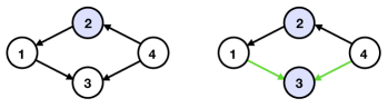
Figure 1: (Left). $\{1\}$ and $\{4\}$ are d-separated by $\{2\}$, as both paths are inactive given $\{2\}$. (Right). $\{1\}$ and $\{4\}$ are not d-separated by $\{2,3\}$, as the path $1\to 3\operatorname{\leftarrow}4$ is active given $\{2,3\}$ by the collider $3$.

Random variables $X_{A},X_{B}$ are conditionally independent given $X_{C}$ if $A{\mathrel{\mspace{2.0mu}\perp\mspace{-12.0mu}\perp\mspace{2.0mu}}}B\mid_{\mathcal{H}}C$ (Dawid,, 1979). We write $I_{\mathcal{H}}(A,B\mid C)=1$ if $X_{A},X_{B}$ are conditionally independent given $X_{C}$ and $I_{\mathcal{H}}(A,B\mid C)=0$ otherwise. Under the so-called faithfulness assumption, the reverse is also true, i.e., all CI relations of $\mathbb{P}$ are implied by d-separation in $\mathcal{H}$. We thus have

$$A{\mathrel{\mspace{2.0mu}\perp\mspace{-12.0mu}\perp\mspace{2.0mu}}}B\mid_{\mathcal{H}}C\Longleftrightarrow I_{\mathcal{H}}(A,B\mid C)=1.$$

If any set among $A,B,C$ only contains one node, e.g., $A=\{a\}$, we write $a{\mathrel{\mspace{2.0mu}\perp\mspace{-12.0mu}\perp\mspace{2.0mu}}}B\mid_{\mathcal{H}}C$ and $I_{\mathcal{H}}(a,B\mid C)$ for simplicity.

For two DAGs $\mathcal{H}$ and $\mathcal{G}$, if all d-separations in $\mathcal{G}$ are in $\mathcal{H}$, i.e., $A{\mathrel{\mspace{2.0mu}\perp\mspace{-12.0mu}\perp\mspace{2.0mu}}}B\mid_{\mathcal{G}}C\Rightarrow A{\mathrel{\mspace{2.0mu}\perp\mspace{-12.0mu}\perp\mspace{2.0mu}}}B\mid_{\mathcal{H}}C$, then $\mathcal{G}$ is called an independence map of $\mathcal{H}$ and write $\mathcal{H}\leq\mathcal{G}$. It is minimal if removing any edge from $\mathcal{G}$ breaks this relation.

Independence Query Oracles

In our work, we assume throughout that the causal DAG $\mathcal{H}$ is unknown. But we assume faithfulness and access to enough observational samples to determine if $X_{A},X_{B}$ are conditionally independent given $X_{C}$, i.e., $I_{\mathcal{H}}(A,B\mid C)$, when queried. We call this the independence query oracle.

By the above discussion, we know that the value of $I_{\mathcal{H}}(A,B\mid C)$ equivalently implies properties of the DAG $\mathcal{H}$, i.e., whether $A{\mathrel{\mspace{2.0mu}\perp\mspace{-12.0mu}\perp\mspace{2.0mu}}}B\mid_{\mathcal{H}}C$. Therefore in the following, we also use $I_{\mathcal{H}}(A,B\mid C)$ to denote that $A$ and $B$ are d-separated by $C$ in $\mathcal{H}$ (with a slight misuse of notation).

2.3 Markov Equivalence Classes

With observational data and no additional parametric assumptions, the DAG $\mathcal{H}$ is generally only identifiable up to its Markov equivalence class (MEC) (Verma and Pearl,, 1990). Two DAGs $\mathcal{H},\mathcal{G}$ are in the same MEC if any positive distribution that factorizes according to $\mathcal{H}$ also factorizes according to $\mathcal{G}$. For any DAG $\mathcal{G}$, we denote its MEC by $[\mathcal{G}]$. It is known that $\mathcal{H}\in[\mathcal{G}]$ if and only if $\mathcal{H},\mathcal{G}$ share the same skeleton and v-structures (Andersson et al.,, 1997). The essential graph $\mathcal{E}(\mathcal{G})$ is a partially directed graph that fully characterizes $[\mathcal{G}]$, where an edge $i\to j$ is directed if $i\to j$ in every DAG in $[\mathcal{G}]$, and an edge $u\sim v$ is undirected if there exists two DAGs $\mathcal{G}_{1},\mathcal{G}_{2}\in[\mathcal{G}]$ such that $i\to j$ in $\mathcal{G}_{1}$ and $i\operatorname{\leftarrow}j$ in $\mathcal{G}_{2}$. We define $\operatorname{pa}_{[\mathcal{G}]}(i)$ and $\operatorname{ch}_{[\mathcal{G}]}(i)$ as directed parents and children of $i$ in $\mathcal{E}(\mathcal{G})$, respectively. We denote $\operatorname{adj}_{[\mathcal{G}]}(i)=\{j:j-i\in\mathcal{E}(\mathcal{G})\}$ as the remaining nodes with undirected edges to $i$ in $\mathcal{E}(\mathcal{G})$.

As illustrated in Fig. 2, our results are in terms of graph parameters of an MEC $[\mathcal{G}]$, which are defined based on its essential graph $\mathcal{E}(\mathcal{G})$. An undirected clique is a clique in $\mathcal{E}(\mathcal{G})$ after removing all its directed edges, where $s$ is the size of the maximum undirected clique.

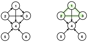
Figure 2: (Left). DAG $\mathcal{G}$. (Right). Essential graph $\mathcal{E}(\mathcal{G})$ representing $[\mathcal{G}]$. In $\mathcal{E}(\mathcal{G})$, the maximum undirected clique has size $s=3$ (highlighted in green). The maximum in-degree of $\mathcal{G}$ is $d=5$ (on node $4$).

We now state some useful properties about essential graphs from Andersson et al., (1997) and Wienöbst et al., (2021). First, every essential graph is a chain graph with chordal chain components. Therefore any undirected clique of the essential graph must belong to a unique chordal chain components. Second, orientations in one chain component do not affect orientations in other components. Third, any clique within a chain component can be made most upstream of this chain component (i.e., all edges in this chain component are pointing out from this clique) and the edge directions of this clique can be made arbitrary as long as there is no cycle within the clique. These results imply, if we denote the maximum undirected clique of $\mathcal{E}(\mathcal{G})$ by $\mathcal{S}$, that for any acylic completion of $\mathcal{S}$, there is $\mathcal{G}_{1}\in[\mathcal{G}]$ that contains it; moreover, $\mathcal{S}$ is most upstream of $\mathcal{G}_{1}$.

3 MAIN RESULTS

As highlighted in the introduction, our work formally explores the testing aspects of causal discovery. We now provide a precise definition of the testing problem.

Testing Problem

Given a specific MEC $[\mathcal{G}]$ as well as independence-query-oracle access to an observational distribution $\mathbb{P}$ respecting a hidden causal DAG $\mathcal{H}$, design an algorithm to test if $\mathcal{H}\in[\mathcal{G}]$ while minimizing the number of CI tests queried.

Throughout our work, we focus on the worst-case query complexity for causal DAGs. Our query complexity bounds are articulated in forms of the parameters of the essential graph $\mathcal{E}(\mathcal{G})$, which succinctly characterizes the specified MEC $[\mathcal{G}]$. In the following, we present our two key findings, which establish matching lower and upper bounds on the query complexity of the testing problem. We start with our lower bound result.

Theorem 1.

Given a specific MEC $[\mathcal{G}]$, there exists a hidden DAG $\mathcal{H}$ such that any algorithm requires at least $\exp(\Omega(s))$ CI tests to test if $\mathcal{H}\in[\mathcal{G}]$. Here, $s$ is the size of the maximum undirected clique in $\mathcal{E}(\mathcal{G})$.

It is worth noting that for the learning task, which entails the recovery of $[\mathcal{H}]$, algorithms typically exhibit a query complexity that is at least an exponential function of the maximum in-degree of the essential graph. Since the size of the maximum undirected clique is always upper bounded by the maximum degree, our lower bound result suggests that the testing problem might be easier compared to learning. We confirm this by the following result, which provides an algorithm that resolves the testing problem with a query count matching the lower bound.

Theorem 2.

Given a specific MEC $[\mathcal{G}]$ and any hidden DAG $\mathcal{H}$, there exists an algorithm that runs in polynomial time and performs at most $\exp(O(s)+O(\log n))$ number of CI tests to test if $\mathcal{H}\in[\mathcal{G}]$.

Our bounds exhibit instance-dependent tightness for any given MEC. In the remaining part of this section, we will provide a concise overview of the techniques used to establish our results.

3.1 Overview of Techniques

Lower Bound

We first discuss our lower bound result for the simple case where $\mathcal{E}(\mathcal{G})$ is an undirected clique. Let the hidden causal graph be obtained by removing an edge $i\to j$ from a DAG $\mathcal{G}$ that belongs to the MEC, where $\operatorname{pa}_{\mathcal{G}}(i)=\varnothing$. Given such $\mathcal{H}$, we can show that the only set of independence test queries that differentiate $[\mathcal{H}]$ from $[\mathcal{G}]$ are of the form:

$$i{\mathrel{\mspace{2.0mu}\perp\mspace{-12.0mu}\perp\mspace{2.0mu}}}j\mid\operatorname{ch}_{\mathcal{G}}(i)\cap\operatorname{pa}_{\mathcal{G}}(j).$$

As any subset of nodes in the clique could lie between $i$ and $j$ for some $\mathcal{G}$ in the MEC, we immediately get a worst-case lower bound of $\binom{s}{\lceil s/2\rceil-1}=\exp(\Omega(s))$.

The above result naturally extends to MECs with general $\mathcal{E}(\mathcal{G})$ by utilizing the properties that we discussed in Section 2.3. Namely, any clique in a connected component of the specified MEC could be made most upstream, and therefore we could ignore all the remaining nodes in that component. A formal proof of this result is provided in Section 4.

We remark here that our result is an instance-dependent bound with respect to (any) $\mathcal{G}$, which is more general than considering only fully connected $\mathcal{G}$’s.

Upper Bound

We first show that if the specified MEC contains additional independence relations that are not in the hidden DAG, then this can be detected with $O(n^{2})$ queries. This holds because, for each $i\not\sim j$ in the essential graph $\mathcal{E}(\mathcal{G})$, one can easily find a set $C$ such that $i{\mathrel{\mspace{2.0mu}\perp\mspace{-12.0mu}\perp\mspace{2.0mu}}}j\mid_{\mathcal{G}}C$. However, if $I_{\mathcal{H}}(i,j\mid C)=0$, then this query quickly reveals $\mathcal{H}\notin[\mathcal{G}]$. On the other hand, if $I_{\mathcal{H}}(i,j\mid C)=1$, then $i{\mathrel{\mspace{2.0mu}\perp\mspace{-12.0mu}\perp\mspace{2.0mu}}}j\mid_{\mathcal{H}}C$. Since d-separation relations exhibit axiomatic properties, these can be used to show $\mathcal{H}\leq\mathcal{G}$. We call such tests canonical CI tests, which we formally define in Section 3.2.

Along with these CI tests, we define another type of canonical CI tests utilitizing the undirected cliques in $\mathcal{E}(\mathcal{G})$. These two types of tests together resolve the case where the hidden graph contains a missing edge in the specified MEC. In particular, if $\mathcal{H}$ is missing an edge and $\mathcal{H}\leq\mathcal{G}$, then a result by Chickering, (2002) proving Meek’s conjecture (Meek,, 1995) implies that there is a DAG $\mathcal{H}^{\prime}$ such that $\mathcal{H}\leq\mathcal{H}^{\prime}\leq\mathcal{G}$ and $\mathcal{H}^{\prime}$ is one-edge away from some $\mathcal{G}^{\prime}\in[\mathcal{G}]$. Using the local Markov property (Lauritzen,, 1996), this missing edge $i\sim j$ can be detected by $i{\mathrel{\mspace{2.0mu}\perp\mspace{-12.0mu}\perp\mspace{2.0mu}}}j\mid_{\mathcal{H}}C$ for some set $C$ that contains parents of one of the nodes $i,j$. We then show that this set $C$ can be obtained via an undirected clique within $\mathcal{E}(\mathcal{G})$, if the hidden graph passes the canonical CI tests defined next. Therefore we can detect this case with $\exp(O(s))$ number of CI queries.

These results imply that we only need to consider the remaining case where $\operatorname{skel}(\mathcal{H})=\operatorname{skel}(\mathcal{G})$. When the skeleta align, we show that it is easy to test whether the v-structures align. Detailed algorithms and proofs are provided in Section 5. Additionally, we provide a geometric view of these results in Section 6.

3.2 Canonical CI Test Oracles

We now define two types of canonical CI test oracles (illustrated in Fig. 3) that will be used in our algorithms for the testing problem of whether $\mathcal{H}\in[\mathcal{G}]$.

Definition 3 (Class-I CI Test).

For $i\not\sim j$ in $[\mathcal{G}]$, there is $i{\mathrel{\mspace{2.0mu}\perp\mspace{-12.0mu}\perp\mspace{2.0mu}}}j\mid_{\mathcal{G}}\operatorname{pa}_{\mathcal{G}}(i)\setminus\{j\}$, assuming $j\notin\operatorname{de}_{\mathcal{G}}(i)$ without loss of generality. Test if $I_{\mathcal{H}}(i,j\mid\operatorname{pa}_{\mathcal{G}}(i)\setminus\{j\})=1$.

We make a few remarks on these tests. First, the d-separation claim about $\mathcal{G}$ comes from the local Markov property (Lauritzen,, 1996). Second, these tests are equivalent to testing if the underlying joint distribution $\mathbb{P}$ factorizes with respect to $\mathcal{G}$, which is a necessary condition for $\mathcal{H}\in[\mathcal{G}]$.

Definition 4 (Class-II CI Test).

For $i\sim j$ in $[\mathcal{G}]$, there is $i\mathrel{{\not\perp\mspace{-12.0mu}\perp}}j\mid_{\mathcal{G}}\big{(}\operatorname{pa}_{[\mathcal{G}]}(i)\cup C\big{)}\setminus\{j\}$ for all undirected cliques $C\subseteq\operatorname{adj}_{[\mathcal{G}]}(i)$. Test if $I_{\mathcal{H}}\big{(}i,j\mid\big{(}\operatorname{pa}_{[\mathcal{G}]}(i)\cup C\big{)}\setminus\{j\}\big{)}=0$.

(a) Class-I CI Test

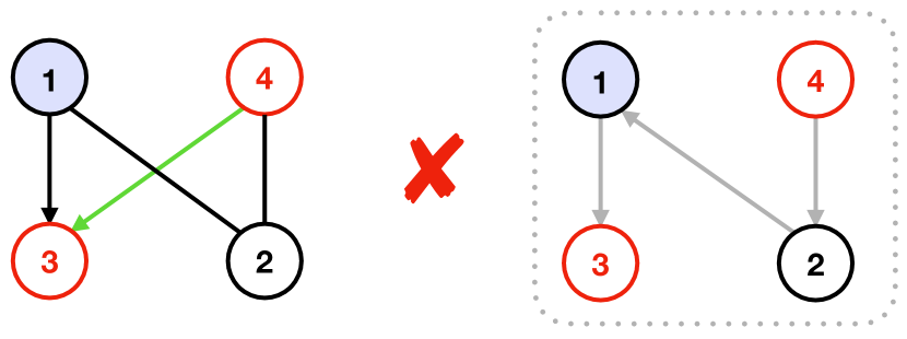
(b) Class-II CI Test

Figure 3: Examples of canonical CI tests. The given MEC $\mathcal{G}$ is on the left, and the hidden $\mathcal{H}$ is on the right. (a) Class-I CI test $1{\mathrel{\mspace{2.0mu}\perp\mspace{-12.0mu}\perp\mspace{2.0mu}}}4\mid 2$ agrees between $\mathcal{H},\mathcal{G}$. (b) Class-II CI test $3{\mathrel{\mspace{2.0mu}\perp\mspace{-12.0mu}\perp\mspace{2.0mu}}}4\mid 1$ disagrees between $\mathcal{H},\mathcal{G}$.

We will show in Section 5 that if all the class-I and class-II canonical independence queries are satisfied in the hidden graph $\mathcal{H}$, then $\mathcal{H}$ has to be in $[\mathcal{G}]$.

4 LOWER BOUND

In Section 3.1, we explained how the lower bound example is constructed; namely by considering a DAG $\mathcal{H}$ that is missing one undirected edge in $[\mathcal{G}]$. We now provide steps towards Theorem 1. All omitted proofs can be found in Appendix 2.

A key lemma is to show that when two DAGs are very similar, namely, one is missing only an edge that is undirected in the MEC of the other, they share certain active/inactive paths.

Lemma 5.

Let $\mathcal{G}_{1}$ and $\mathcal{G}_{2}$ be two DAGs such that $\mathcal{G}_{1}$ differs from $\mathcal{G}_{2}$ only by missing one edge $i\to j$, which is undirected in $\mathcal{E}(\mathcal{G}_{2})$. Let $\mathcal{P}:a-\dots-b$ be a common path shared by $\mathcal{G}_{1}$ and $\mathcal{G}_{2}$. For any arbitrary set $C\subseteq[n]\setminus\{a,b\}$,

1. if $\mathcal{P}$ is inactive given $C$ in $\mathcal{G}_{2}$, then it must be inactive given $C$ in $\mathcal{G}_{1}$;

2. if $\mathcal{P}$ is active given $C$ in $\mathcal{G}_{2}$, then there is a path connecting $a,b$ that is active given $C$ in $\mathcal{G}_{1}$.

An immediate corollary of this lemma is the following statement about d-separations in such DAGs.

Corollary 6.

Let $\mathcal{G}_{1},\mathcal{G}_{2}$ be two DAGs as in Lemma Lemma. For any nodes $a\neq b\in[n]$ and set $C\subset[n]\setminus\{a,b\}$,

1. if $a{\mathrel{\mspace{2.0mu}\perp\mspace{-12.0mu}\perp\mspace{2.0mu}}}b\mid_{\mathcal{G}_{2}}C$, then $a{\mathrel{\mspace{2.0mu}\perp\mspace{-12.0mu}\perp\mspace{2.0mu}}}b\mid_{\mathcal{G}_{1}}C$;

2. if $a\mathrel{{\not\perp\mspace{-12.0mu}\perp}}b\mid_{\mathcal{G}_{2}}C$ and there is path from $a$ to $b$ in $\mathcal{G}_{1}$ that is active given $C$ in $\mathcal{G}_{2}$, then $a\mathrel{{\not\perp\mspace{-12.0mu}\perp}}b\mid_{\mathcal{G}_{1}}C$.

Proof.

If $a{\mathrel{\mspace{2.0mu}\perp\mspace{-12.0mu}\perp\mspace{2.0mu}}}b\mid_{\mathcal{G}_{2}}C$, then all paths from $a$ to $b$ are inactive given $C$ in $\mathcal{G}_{2}$. Since every path in $\mathcal{G}_{1}$ is a path in $\mathcal{G}_{2}$, all paths from $a$ to $b$ are inactive given $C$ in $\mathcal{G}_{1}$ as well by Lemma Lemma (1). Thus $a{\mathrel{\mspace{2.0mu}\perp\mspace{-12.0mu}\perp\mspace{2.0mu}}}b\mid_{\mathcal{G}_{1}}C$.

If $a\mathrel{{\not\perp\mspace{-12.0mu}\perp}}b\mid_{\mathcal{G}_{2}}C$ and there is path from $a$ to $b$ in $\mathcal{G}_{1}$ that is active given $C$ in $\mathcal{G}_{2}$, this would be a common path shared by $\mathcal{G}_{1},\mathcal{G}_{2}$. By Lemma Lemma (2), there must be a path connecting $a,b$ that is active given $C$ in $\mathcal{G}_{1}$. Thus $a\mathrel{{\not\perp\mspace{-12.0mu}\perp}}b\mid_{\mathcal{G}_{1}}C$. ∎

Using Corollary Lemma, we can now show that if a CI test disagrees between such two similar DAGs, then the conditioned set must intersect a particular neighborhood of the missing edge.

Lemma 7.

Let $\mathcal{G}_{1},\mathcal{G}_{2}$ be two DAGs that differ by a missing edge $i\to j$ as in Lemma Lemma. Denote the maximal undirected clique in $\mathcal{G}_{2}$ containing $i,j$ by $\mathcal{S}$. Then $I_{\mathcal{G}_{1}}(A,B\mid C)\neq I_{\mathcal{G}_{2}}(A,B\mid C)$ only if $A{\mathrel{\mspace{2.0mu}\perp\mspace{-12.0mu}\perp\mspace{2.0mu}}}B\mid_{\mathcal{G}_{1}}C$, $A\mathrel{{\not\perp\mspace{-12.0mu}\perp}}B\mid_{\mathcal{G}_{2}}C$, and

$$\left(\operatorname{pa}_{\mathcal{G}_{2}}(j)\cap\operatorname{ch}_{\mathcal{G}_{2}}(i)\right)\cap\mathcal{S} \subseteq$$

$$C\cap\mathcal{S} \subseteq\left(\operatorname{pa}_{\mathcal{G}_{2}}(j)\setminus\{i\}\right)\cap\mathcal{S}.$$

This result lays the crucial step for Theorem 1, since the particular neighborbood of the missing edge can require $\exp(\Omega(s))$ tests to be identified in the worst case.

Proof of Theorem 1..

Let $\mathcal{S}$ be the maximum undirected clique in $\mathcal{E}(\mathcal{G})$ with size $s$. Denote $i,j$ as the $1$-st and $\lfloor s/2\rfloor$-th nodes in the topological order of nodes of $\mathcal{S}$ in the DAG $\mathcal{G}$. Let $K$ be the set of all nodes that lie in between $i$ and $j$ in the topological order.

Let $\mathcal{H}$ be the DAG obtained by removing $i\to j$ from $\mathcal{G}$. We will show that any algorithm requires at least $\binom{s}{\lceil s/2\rceil-1}$ CI tests to verify $\mathcal{H}\notin[\mathcal{G}]$ in the worst case.

Since $\mathcal{S}$ is undirected, $i\to j$ must be undirected in $\mathcal{E}(\mathcal{G})$. Using Lemma Lemma for $\mathcal{G}$ and $\mathcal{H}$, any disjoint sets $A,B,C$ satisfy that $I_{\mathcal{H}}(A,B\mid C)\neq I_{\mathcal{G}}(A,B\mid C)$ only if $C\cap\mathcal{S}=K$ (i.e., the nodes of $\mathcal{S}$ that are in $C$ are exactly $K$), since

$$K=\left(\operatorname{pa}_{\mathcal{G}}(j)\cap\operatorname{ch}_{\mathcal{G}}(i)\right)\cap\mathcal{S}\subseteq C\cap\mathcal{S}$$

$$\subseteq\left(\operatorname{pa}_{\mathcal{G}}(j)\setminus\{i\}\right)\cap\mathcal{S} =K.$$

Therefore any CI test of $A,B$ given $C$ would agree between $\mathcal{H}$ and $\mathcal{G}$ if $C\cap\mathcal{S}\neq K$. However, since $\mathcal{S}$ is an undirected clique in $\mathcal{E}(\mathcal{G})$, its nodes can be ordered arbitrarily to obtain a valid DAG in $[\mathcal{G}]$. Therefore, no additional information can be learned about $i,j$ by performing CI tests until $C\cap\mathcal{S}=K$. Since all topological orders can be valid, it can take $\binom{s}{|K|}=\binom{s}{\lceil s/2\rceil-1}$ CI tests until $C\cap\mathcal{S}=K$ in the worst case. ∎

We make some final remarks about Theorem 1. First, it is a worst-case result over all possible hidden graphs $\mathcal{H}$. Second, since $s$ depends on $[\mathcal{G}]$, this lower bound is instance-wise with respect to the MEC of interest.

5 UPPER BOUND

We now present our upper bound results. All omitted proofs can be found in Appendix 3.

We begin by presenting our algorithm for testing. Our algorithm is built upon the canonical CI tests introduced in Section 3.2 (Definitions 3,4).

1:Input: MEC $[\mathcal{G}]$ and independence-query oracle access to hidden DAG $\mathcal{H}$.

2:Output: whether hidden $\mathcal{H}$ belongs to $[\mathcal{G}]$.

3:Perform all class-I CI tests with respect to $\mathcal{G}$ and $\mathcal{H}$ sequentially; return False once $\mathcal{H}$ fails.

4:for $i\sim j$ in $[\mathcal{G}]$ do

5:   for undirected clique $C$ in $\operatorname{adj}_{[\mathcal{G}]}(i)$ do

6:       Test $I_{\mathcal{H}}\big{(}i,j\mid\big{(}\operatorname{pa}_{[\mathcal{G}]}(i)\cup C\big{)}\setminus\{j\}\big{)}$.

7:       return False if independence.

8:    Perform line 4-6 for $j$.

9:return True.

Algorithm 1 Membership Testing in MEC.

Note that the total number of maximal undirected cliques in $[\mathcal{G}]$ cannot exceed $n$ (see Appendix 3). Since each undirected clique must belong to some maximal undirected clique whose size $\leq s$, the total number of undirected cliques cannot exceed $n\cdot 2^{s}$. Thus, the total number of class-II CI tests performed is bounded by $n^{3}\cdot 2^{s}=\exp(O(s)+O(\log n))$.

We prove the correctness of Algorithm 1 by showing that if $\mathcal{H}\notin[\mathcal{G}]$, then $\mathcal{H}$ fails at least one of the class-I or class-II CI tests. It is clear from the definition that $\mathcal{H}$ will pass all these CI tests when $\mathcal{H}\in[\mathcal{G}]$.

5.1 Class-I CI Tests Imply $\mathcal{H}\leq\mathcal{G}$

We first show that passing class-I CI tests implies $\mathcal{H}\leq\mathcal{G}$, i.e., all CI relations in $\mathcal{G}$ must hold in $\mathcal{H}$.

Lemma 8.

If $\mathcal{H}$ passes all class-I CI tests, then $\mathcal{H}\leq\mathcal{G}$. In particular, this implies $\operatorname{skel}(\mathcal{H})\subseteq\operatorname{skel}(\mathcal{G})$.

Proof.

Passing all class-I CI tests with respect to $\mathcal{G}$ and $\mathcal{H}$ implies that the joint distribution $\mathbb{P}$ factorizes according to $\mathcal{G}$, which in turn implies that $\mathbb{P}$ satisfies all CI relations given by d-separation in $\mathcal{G}$. Since $\mathbb{P}$ is faithful to $\mathcal{H}$, it follows that $\mathcal{H}\leq\mathcal{G}$. Additionally, if there is an edge $i\sim j$ in $\mathcal{H}$ but not in $\mathcal{G}$, assuming $j\not\in\operatorname{de}_{\mathcal{G}}(i)$, we obtain $i{\mathrel{\mspace{2.0mu}\perp\mspace{-12.0mu}\perp\mspace{2.0mu}}}j\mid_{\mathcal{G}}\operatorname{pa}_{\mathcal{G}}(i)\setminus\{j\}$ but $i\mathrel{{\not\perp\mspace{-12.0mu}\perp}}j\mid_{\mathcal{H}}\operatorname{pa}_{\mathcal{G}}(i)\setminus\{j\}$; a contradiction to $\mathcal{H}\leq\mathcal{G}$. ∎

Note that the consequence of class-I CI tests in Lemma 8 essentially follows from the equivalence between the local and global Markov properties (Pearl,, 1988), which establishes that all d-separation statements can be deduced by only a few (local) statements.

5.2 Class-II CI Tests Imply $\operatorname{skel}(\mathcal{H})=\operatorname{skel}(\mathcal{G})$

Suppose that $\mathcal{H}$ passes all class-I CI tests; we now show that passing all class-II CI tests implies $\operatorname{skel}(\mathcal{H})=\operatorname{skel}(\mathcal{G})$.

Using Lemma 8, we obtain $\mathcal{H}\leq\mathcal{G}$ and $\operatorname{skel}(\mathcal{H})\subseteq\operatorname{skel}(\mathcal{G})$. If $\operatorname{skel}(\mathcal{H})\neq\operatorname{skel}(\mathcal{G})$, then there exists a CI relation that holds in $\mathcal{H}$ but not in $\mathcal{G}$. In this case, we can construct a “middle” DAG that lies between $\mathcal{H},\mathcal{G}$ whose skeleton differs from $\operatorname{skel}(\mathcal{G})$ by only one edge. This construction is a direct consequence based on the proof by Chickering, (2002) of Meek’s conjecture (Meek,, 1995).

Proposition 9.

If $\mathcal{H}\leq\mathcal{G}$ and $\operatorname{skel}(\mathcal{H})\subsetneq\operatorname{skel}(\mathcal{G})$, then there exist a DAG $\mathcal{H}^{\prime}$ such that $\mathcal{H}\leq\mathcal{H}^{\prime}\leq\mathcal{G}$ and $\mathcal{H}^{\prime}$ is missing one edge in $\mathcal{G}^{\prime}$ for some $\mathcal{G}^{\prime}\in[\mathcal{G}]$.

Then it only remains to find the existence of a CI relation that holds in $\mathcal{H}^{\prime}$ (which holds in $\mathcal{H}$ since $\mathcal{H}\leq\mathcal{H}^{\prime}$) but not in $\mathcal{G}^{\prime}$ (or equivalently, $\mathcal{G}$, since $\mathcal{G}^{\prime}\in[\mathcal{G}]$). This can be detected by class-II CI tests. The intuition for this is provided in the following lemma.

Lemma 10.

For any $i$ in $\mathcal{G}^{\prime}\in[\mathcal{G}]$, there is $\operatorname{pa}_{\mathcal{G}^{\prime}}(i)=\operatorname{pa}_{[\mathcal{G}]}(i)\cup C$ for some undirected clique $C\subseteq\operatorname{adj}_{[\mathcal{G}]}(i)$.

An immediate consequence of these two results is the following corollary.

Corollary 11.

If $\mathcal{H}$ passes all class-I and class-II CI tests, then $\operatorname{skel}(\mathcal{H})=\operatorname{skel}(\mathcal{G})$.

Proof.

Suppose $\operatorname{skel}(\mathcal{H})\neq\operatorname{skel}(\mathcal{G})$; then by Lemma 8 and Proposition 9, we know there exists $\mathcal{H}^{\prime}$ and $\mathcal{G}^{\prime}\in[\mathcal{G}]$ such that $\mathcal{H}\leq\mathcal{H}^{\prime}\leq\mathcal{G}$ and $\mathcal{H}^{\prime}$ differs from $\mathcal{G}^{\prime}$ by one missing edge. Suppose the missing edge is $j\to i$ in $\mathcal{G}^{\prime}$, then $i{\mathrel{\mspace{2.0mu}\perp\mspace{-12.0mu}\perp\mspace{2.0mu}}}j\mid_{\mathcal{H}^{\prime}}\operatorname{pa}_{\mathcal{H}^{\prime}}(i)$. Note that $\operatorname{pa}_{\mathcal{H}^{\prime}}(i)=\operatorname{pa}_{\mathcal{G}^{\prime}}(i)\setminus\{j\}$. By Lemma 10, $\operatorname{pa}_{\mathcal{G}^{\prime}}(i)=\operatorname{pa}_{[\mathcal{G}]}(i)\cup C$ for some undirected clique $C\subseteq\operatorname{adj}_{[\mathcal{G}]}(i)$. Therefore $i{\mathrel{\mspace{2.0mu}\perp\mspace{-12.0mu}\perp\mspace{2.0mu}}}j\mid_{\mathcal{H}^{\prime}}\operatorname{pa}_{[\mathcal{G}]}(i)\cup C\setminus\{j\}$. Since $\mathcal{H}\leq\mathcal{H}^{\prime}$, we have $i{\mathrel{\mspace{2.0mu}\perp\mspace{-12.0mu}\perp\mspace{2.0mu}}}j\mid_{\mathcal{H}}\operatorname{pa}_{[\mathcal{G}]}(i)\cup C\setminus\{j\}$. This means that $\mathcal{H}$ fails a class-II CI test; a contradiction. ∎

We are now ready to prove our main theorem.

Proof of Theorem 2.

If $\mathcal{H}$ fails any of the class-I or class-II tests, then $\mathcal{H}\notin[\mathcal{G}]$. Thus, suppose that $\mathcal{H}$ passes all the class-I and class-II tests. Then by Corollary 11, we obtain $\operatorname{skel}(\mathcal{H})=\operatorname{skel}(\mathcal{G})$. For any triplets $i\sim k\sim j$ such that $i\not\sim j$ in $\mathcal{G}$, assume that $j\not\in\operatorname{de}_{\mathcal{G}}(i)$ without loss of generality. If $i\sim k\sim j$ is a v-structure in $\mathcal{G}$, then $k\not\in\operatorname{pa}_{\mathcal{G}}(i)$. Consequently, it is a v-structure in $\mathcal{H}$, since it passes the class-I test of $i{\mathrel{\mspace{2.0mu}\perp\mspace{-12.0mu}\perp\mspace{2.0mu}}}j\mid_{\mathcal{H}}\operatorname{pa}_{\mathcal{G}}(i)\setminus\{j\}$ in Definition 3. Similarly if it is not a v-structure in $\mathcal{G}$, then it is not a v-structure in $\mathcal{H}$. Thus $\mathcal{H},\mathcal{G}$ also share the same set of v-structures. Hence it holds that $\mathcal{H}\in[\mathcal{G}]$.

Since the total number of class-I and class-II tests sum up to $\exp(O(s)+O(\log n))$, we arrive at the result. ∎

6 DAG ASSOCIAHEDRON

In this section, we map our findings onto the DAG associahedron (Mohammadi et al.,, 2018), thereby providing a geometric interpretation of our results. Using edgewalks on the DAG associahedron, we establish in Section 6.1 that (1) testing is stricly harder than learning, (2) how our testing algorithm can aid learning with potentially fewer CI tests.

We begin by introducing the DAG associahedron. Let $\mathcal{A}_{n}$ denote the permutohedron on $n$ elements, i.e., the convex polytope in $\mathbb{R}^{n}$ with vertices corresponding to all permutation vectors of size $n$. Two vertices on $\mathcal{A}_{n}$ are connected by an edge if and only if their corresponding permutations differ by an adjacent transposition. The DAG associahedron $\mathcal{A}_{n}(\mathcal{H})$ with respect to a DAG $\mathcal{H}$ is obtained by contracting edges in $\mathcal{A}_{n}$ corresponding to d-separations in $\mathcal{H}$. Namely, the edge between vertices $(\pi_{1},\dots,\pi_{i},\pi_{i+1},\dots,\pi_{n})$ and $(\pi_{1},\dots,\pi_{i+1},\pi_{i},\dots,\pi_{n})$ is contracted when $\pi_{i}{\mathrel{\mspace{2.0mu}\perp\mspace{-12.0mu}\perp\mspace{2.0mu}}}\pi_{i+1}\mid_{\mathcal{H}}\{\pi_{1},\dots,\pi_{i-1}\}$. It was shown that (1) $\mathcal{A}_{n}(\mathcal{H})$ remains a convex polytope (section 4 in Mohammadi et al., (2018)); (2) the vertices of $\mathcal{A}_{n}(\mathcal{H})$ correspond to minimal independence maps of $\mathcal{H}$ that can be obtained via any of the associated permutations before contraction (Theorem 7.1 in Mohammadi et al., (2018)). Fig. 4 illustrates these concepts.

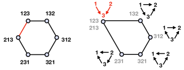
Figure 4: (Left). Permutohedron $\mathcal{A}_{3}$. (Right). DAG associahedron $\mathcal{A}_{3}(1\to 3\operatorname{\leftarrow}2)$. The corresponding DAG and contracted edge are in red.

We can now reinterpret our results using $\mathcal{A}_{n}(\mathcal{H})$.

Testing if $\mathcal{G}$ is on the polytope

Note that as $\mathcal{H}$ and any DAGs in $[\mathcal{H}]$ are minimal independence maps of $\mathcal{H}$, property (2) in the above paragraphs indicates that $\mathcal{H}\in[\mathcal{G}]$ only if $\mathcal{G}$ is a vertex of $\mathcal{A}_{n}(\mathcal{H})$. Therefore the first test is to see if $\mathcal{G}$ is on $\mathcal{A}_{n}(\mathcal{H})$. By Lemma 8, we can test if $\mathcal{G}$ is an independence map of $\mathcal{H}$ by class-I CI tests. To further test if $\mathcal{G}$ is a minimal independence map of $\mathcal{H}$, one only needs to perform $O(n^{2})$ tests to see if any edge in $\mathcal{G}$ is removable. Therefore this gives us a way to rule out the case when $\mathcal{G}$ is not on $\mathcal{A}_{n}(\mathcal{H})$.

Testing if $\mathcal{G}$ is a sparsest DAG

Once we establish that $\mathcal{G}$ is on $\mathcal{A}_{n}(\mathcal{H})$, we can test if $\operatorname{skel}(\mathcal{G})=\operatorname{skel}(\mathcal{H})$ by testing if $\mathcal{G}$ is a sparsest DAG on $\mathcal{A}_{n}(\mathcal{H})$ (since no minimal independence map of $\mathcal{H}$ can be sparser than $\operatorname{skel}(\mathcal{H})$). If $\mathcal{G}$ is not sparsest, then it was shown that one can find a strictly sparser DAG $\mathcal{H}_{1}$ such that $\mathcal{H}\leq\mathcal{H}_{1}\leq\mathcal{G}$ by a specific sequence of edgewalks from $\mathcal{G}$ on $\mathcal{A}_{n}(\mathcal{H})$ (Proposition 8(b) in Solus et al., (2021)). On the contrary, if no such edgewalks exists, then one can conclude that $\mathcal{G}$ is sparsest. Concretely, each edgewalk corresponds to flipping a covered edge in the starting DAG, obtaining a topological order of the flipped DAG, and finding the minimal independence map of this topological order via $O(n^{2})$ CI tests.

Note that this existence result does not imply any non-trivial upper bounds on the number of edgewalks required before finding a sparser DAG. One way to see this is by considering the neighborhood of a sparsest $\mathcal{H}$. Since all DAGs in $[\mathcal{H}]$ are on $\mathcal{A}_{n}(\mathcal{H})$ and one can traverse from one to another via a sequence of covered edge flips (Chickering,, 1995), they are all connected on $\mathcal{A}_{n}(\mathcal{H})$ via the aforementioned edgewalks. Therefore a trivial computation following the above strategy sums up to $O(n^{2})\cdot|[\mathcal{H}]|$ CI tests for verifying that $\mathcal{H}$ is sparsest. Here, $|[\mathcal{H}]|$ is the number of DAGs in the MEC, which can be $\exp(\Omega(n))$ regardless of the maximal undirected clique size $s$ (see Appendix 4).

In comparison, our results in Proposition 9 and Lemma 10 establish that we can skip a lot of edgewalks by directly performing class-II CI tests, which entails no more than $\exp(O(s)+O(\log n))$ CI tests. Upon testing if $\operatorname{skel}(\mathcal{H})=\operatorname{skel}(\mathcal{G})$, it is easy to test if $\mathcal{H}\in[\mathcal{G}]$ following our proof of Theorem 2.

6.1 Learning vs. Testing

By the discussion above, the problem of learning $[\mathcal{H}]$ can be seen as identifying a sparsest vertex of the DAG associahedron $\mathcal{A}_{n}(\mathcal{H})$, whereas the problem of testing if $[\mathcal{G}]=[\mathcal{H}]$ corresponds to verifying if $\mathcal{G}$ is a sparsest vertex. In this regard, it is evident that testing is strictly easier than learning, unless one stumbled upon the correct $[\mathcal{H}]$ at the initial round of learning.

Note that when $\mathcal{G}$ is not sparsest, the existence results discussed above establish that one can walk along the edges of $\mathcal{A}_{n}(\mathcal{H})$ to a strictly sparser DAG. Therefore one can build a greedy search algorithm over $\mathcal{A}_{n}(\mathcal{H})$ to learn $[\mathcal{H}]$. GSP (Solus et al.,, 2021) does this by searching for the sparsest permutations; Lam et al., (2022) and Andrews et al., (2023) showed that certain edgewalks can be skipped by considering traversals of permutations that are different from GSP. In comparison, our results indicate that instead of edgewalks on the DAG associahedron, one can directly arrive at a strictly sparser DAG via class-II CI tests. When the starting DAG belongs to an MEC of large size but has very small undirected cliques, these tests can be much more efficient than edgewalks. Thus in these cases, adopting our strategy may aid learning with potentially fewer CI tests.

7 DISCUSSION

In this work, we introduced the testing problem of causal discovery. We established matching lower and upper bounds on the number of conditional independence tests required to determine if a hidden causal graph, which can be queried using conditional independence tests, belongs to a specified Markov equivalence class. There are several interesting future directions stemming from this work. These include deriving bounds that generalize our results to cyclic graphs. While our work focused on testing if a hidden causal graph belongs to a specified MEC using observational data, it would also be of interest to explore extensions of testing in the presence of interventional data.

Furthermore, it would also be valuable to establish sample complexity bounds and statistical evaluations for the testing problem. As our results provide a binary answer, it will be relevant for real-world scenarios to establish non-binary scores, e.g., measuring how well the given MEC represents the hidden DAG. Another problem which aligns naturally with traditional property testing literature is the approximate testing problem: testing if the hidden graph is in the given MEC or $\epsilon$-far-away from it. There could be many different ways for defining $\epsilon$-far-away distances (such as SHD (Acid and de Campos,, 2003; Tsamardinos et al.,, 2006) and SID(Peters and Bühlmann,, 2015)) that are of interest.

Finally, it would be interesting to explore the implications of our results for causal structure learning. This would be particularly relevant in the context of algorithms that perform greedy search either in the space of permutations (such as GSP (Solus et al.,, 2021) and extensions thereof (Lam et al.,, 2022; Andrews et al.,, 2023)) or in the space of MECs (such as GES (Chickering,, 2002)).

Acknowledgements

We thank the anonymous reviewers for helpful comments. J.Z. was partially supported by an Apple AI/ML PhD Fellowship. K.S.  was supported by a fellowship from the Eric and Wendy Schmidt Center at the Broad Institute. The authors were partially supported by NCCIH/NIH (1DP2AT012345), ONR (N00014-22-1-2116), the United States Department of Energy (DOE), Office of Advanced Scientific Computing Research (ASCR), via the M2dt MMICC center (DE-SC0023187), the MIT-IBM Watson AI Lab, and a Simons Investigator Award to C.U.

Appendix A PRELIMINARIES

We remark here that we do not assume causal sufficiency, since the testing problem assumes that the joint distribution is Markov and faithful to some DAG $\mathcal{H}$ (which does not necessarily imply causal sufficiency) and asks if this DAG is contained in a given MEC $[\mathcal{G}]$. This is in contrast to the learning problem, where one cares about the complete causal explanation (Meek,, 1997) and therefore needs to assume e.g., no unobserved causal variables or cycles.

Since all the DAGs in the same Markov equivalence class share the same v-structures, we know that these v-structures are directed in $\mathcal{E}(\mathcal{G})$. In addition, we can orient an additional set of edges using a set of logical relations known as Meek rules (Meek,, 1995).

Proposition 12 (Meek Rules (Meek,, 1995)).

We can infer all directed edges in $\mathcal{E}(\mathcal{G})$ using the following four rules:

1. If $i\rightarrow j\sim k$ and $i\not\sim k$, then $j\rightarrow k$.

2. If $i\rightarrow j\rightarrow k$ and $i\sim k$, then $i\rightarrow k$.

3. If $i\sim j,i\sim k,i\sim l,j\rightarrow k,l\rightarrow k$ and $j\not\sim l$, then $i\rightarrow k$.

4. If $i\sim j,i\sim k,i\sim l,j\leftarrow k,l\rightarrow k$ and $j\not\sim l$, then $i\rightarrow j$.

Figure 5 illustrates Meek rule 1, which we will use in our lower bound proof.

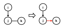
Figure 5: Illustration of Meek rule 1.

Appendix B OMITTED PROOFS OF LOWER BOUND

B.1 Proof of Lemma 5

We now prove Lemma 5, restated below:

Lemma 5.

Let $\mathcal{G}_{1}$ and $\mathcal{G}_{2}$ be two DAGs such that $\mathcal{G}_{1}$ differs from $\mathcal{G}_{2}$ only by a missing edge $i\to j$, which is undirected in $\mathcal{E}(\mathcal{G}_{2})$. Let $\mathcal{P}:a-\dots-b$ be a common path shared by $\mathcal{G}_{1}$ and $\mathcal{G}_{2}$. For any arbitrary set $C\subset[n]\setminus\{a,b\}$,

1. if $\mathcal{P}$ is inactive given $C$ in $\mathcal{G}_{2}$, then it must be inactive given $C$ in $\mathcal{G}_{1}$;

2. if $\mathcal{P}$ is active given $C$ in $\mathcal{G}_{2}$, then there is a path connecting $a,b$ that is active given $C$ in $\mathcal{G}_{1}$.

Proof.

Since $\mathcal{G}_{1}$ differs from $\mathcal{G}_{2}$ by missing one edge and $\mathcal{P}$ is a shared common path, we know that $\mathcal{P}$ has the same set of colliders (and non-colliders) in $\mathcal{G}_{1}$ and $\mathcal{G}_{2}$.

We first show (1). If $\mathcal{P}$ is inactive given $C$ in $\mathcal{G}_{2}$, then either there exists a non-collider $c\in\mathcal{P}\cap C$ or there exists a collider $d\in\mathcal{P}$ such that $\operatorname{\overline{de}}_{\mathcal{G}_{2}}(d)\cap C=\varnothing$. In the first case, $c\in\mathcal{P}\cap C$ is a non-collider in $\mathcal{G}_{1}$ as well. Thus $\mathcal{P}$ is inactive given $C$ in $\mathcal{G}_{1}$. In the second case, since $\mathcal{G}_{1}$ and $\mathcal{G}_{2}$ differ only by one missing edge, it holds that $\operatorname{\overline{de}}_{\mathcal{G}_{1}}(d)\subseteq\operatorname{\overline{de}}_{\mathcal{G}_{2}}(d)$. Therefore $d\in\mathcal{P}$ is a collider in $\mathcal{G}_{1}$ and $\operatorname{\overline{de}}_{\mathcal{G}_{1}}(d)\cap C\subseteq\operatorname{\overline{de}}_{\mathcal{G}_{2}}(d)\cap C=\varnothing$. Thus $\mathcal{P}$ is inactive given $C$ in $\mathcal{G}_{1}$, which proves (1).

We now show (2). Assume to the contrary that $\mathcal{P}$ is active given $C$ in $\mathcal{G}_{2}$ and that there is no path connecting $a,b$ that is active given $C$ in $\mathcal{G}_{1}$.

Let $\mathcal{Q}:a-\dots-b$ be an arbitrary common path shared by $\mathcal{G}_{1}$ and $\mathcal{G}_{2}$ such that it is active given $C$ in $\mathcal{G}_{2}$. For example, $\mathcal{Q}$ can be $\mathcal{P}$. By the assumption, $\mathcal{Q}$ is inactive given $C$ in $\mathcal{G}_{1}$. Since $\mathcal{Q}$ is active given $C$ in $\mathcal{G}_{2}$, every non-collider $c\in\mathcal{Q}$ satisfies $c\notin C$ and every collider $d\in\mathcal{Q}$ satisfies $\operatorname{\overline{de}}_{\mathcal{G}_{2}}(d)\cap C\neq\varnothing$. Since $\mathcal{Q}$ is inactive given $C$ in $\mathcal{G}_{1}$, there exists a collider $d\in\mathcal{Q}$ such that $\operatorname{\overline{de}}_{\mathcal{G}_{1}}(d)\cap C=\varnothing$. This is because all (if any) non-colliders on $\mathcal{Q}$ in $\mathcal{G}_{1}$ must not belong to $C$: since $\mathcal{G}_{1}$ differs from $\mathcal{G}_{2}$ by only one missing edge, any non-collider on $\mathcal{Q}$ in $\mathcal{G}_{1}$ is also a non-collider in $\mathcal{G}_{2}$. By the fact that any non-collider on $\mathcal{Q}$ in $\mathcal{G}_{2}$ is not in $C$, there is no non-collider $c\in\mathcal{Q}\cap C$ in $\mathcal{G}_{1}$. Note that $d$ is also a collider in $\mathcal{G}_{2}$. Therefore it must hold that $\operatorname{\overline{de}}_{\mathcal{G}_{2}}(d)\cap C\neq\varnothing$, otherwise $\mathcal{Q}$ is inactive given $C$ in $\mathcal{G}_{2}$.

Following the arguments in the former paragraph, we know that there must exist a shared collider $d\in\mathcal{Q}$ such that $\operatorname{\overline{de}}_{\mathcal{G}_{2}}(d)\cap C\neq\operatorname{\overline{de}}_{\mathcal{G}_{1}}(d)\cap C=\varnothing$. Since $\operatorname{\overline{de}}_{\mathcal{G}_{2}}(d)\cap C\neq\varnothing$, there exists a directed path $d\rightarrow\cdots\rightarrow c\in C$ in $\mathcal{G}_{2}$; denote $L_{C}(\mathcal{Q})$ as the length of the shortest directed path like this for a given $\mathcal{Q}$.

Consider the following $\mathcal{Q}$. Denote $[\mathcal{P}]$ as the set of all common paths connecting $a,b$ shared by $\mathcal{G}_{1}$ and $\mathcal{G}_{2}$ that are active given $C$ in $\mathcal{G}_{2}$. Since $\mathcal{P}\in[\mathcal{P}]$, we know $[\mathcal{P}]\neq\varnothing$. Let $L$ be the length of the shortest path in $[\mathcal{P}]$. Let $\mathcal{Q}\in[\mathcal{P}]$ be the path among all paths with length $L$ such that $L_{C}(\mathcal{Q})$ is minimized. We will show a contradiction.

Let the nodes $e,d,f,c$ be such that $e\rightarrow d\leftarrow f\in\mathcal{Q}$, $\operatorname{\overline{de}}_{\mathcal{G}_{2}}(d)\cap C\neq\operatorname{\overline{de}}_{\mathcal{G}_{1}}(d)\cap C=\varnothing$, and there is a directed path $\mathcal{L}:d\rightarrow\dots\rightarrow c\in C$ of length $L_{C}(\mathcal{Q})$ in $\mathcal{G}_{2}$. Since $\operatorname{\overline{de}}_{\mathcal{G}_{1}}(d)\cap C=\varnothing$, path $\mathcal{L}$ must not be in $\mathcal{G}_{1}$. Since $\mathcal{G}_{1}$ only differs from $\mathcal{G}_{2}$ by missing one edge $i\rightarrow j$, we know $i\rightarrow j$ must be on $\mathcal{L}$. Suppose $d\rightarrow d_{1}\rightarrow\dots\rightarrow d_{k-1}\to i\to j$ on $\mathcal{L}$ for some integer $k$. Denote for simplicity $d_{k}=i$ and $d_{k+1}=j$.

If $e\not\sim f$ in $\mathcal{G}_{2}$, then $e\rightarrow d\leftarrow f$ construes a v-structure which is directed in $\mathcal{E}(\mathcal{G}_{2})$. If there is $k^{\prime}\in[k+1]$ such that $e-d_{k^{\prime}}-f\in\mathcal{G}_{2}$, then by acyclicity we have $e\rightarrow d_{k^{\prime}}\leftarrow f\in\mathcal{G}_{2}$. Then the path $\mathcal{Q}_{1}:a-\dots-e\to d_{k^{\prime}}\operatorname{\leftarrow}f-\dots-b$ by removing $d$ from $\mathcal{Q}$ and connecting $e$ to $f$ by $d_{k^{\prime}}$ has length $L$ but a directed path from $d_{k^{\prime}}$ to $c$ in $\mathcal{G}_{2}$ of length $L_{C}(\mathcal{Q})-k^{\prime}<L_{C}(\mathcal{Q})$. Note that $\mathcal{Q}_{1}$ is also connecting $a,b$, shared by $\mathcal{G}_{1}$ and $\mathcal{G}_{2}$, and active given $C$ in $\mathcal{G}_{2}$ (since it has the same set of non-colliders as $\mathcal{Q}$ and the additional collider $d_{k^{\prime}}$ has descendant $c\in C$ in $\mathcal{G}_{2}$). This contradicts $\mathcal{Q}$ having $L_{C}(\mathcal{Q})$ minimized. Therefore for all $k^{\prime}\in[k+1]$, node $d_{k^{\prime}}$ will not be adjacent to both $e$ and $f$ in $\mathcal{G}_{2}$. By using Meek rule 1 (Proposition 12) recursively, we know that $d\rightarrow d_{1}\rightarrow\dots\rightarrow d_{k+1}$ is directed in $\mathcal{E}(\mathcal{G}_{2})$. This contradicts $i\to j$ being undirected in $\mathcal{E}(\mathcal{G}_{2})$.

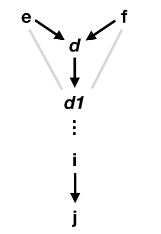
(a) $e\not\sim f$ in $\mathcal{G}_{2}$

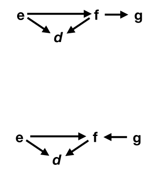
(b) $e\sim f$ in $\mathcal{G}_{2}$

Figure 6: Illustration for the proof of Lemma 5.

If $e\sim f$ in $\mathcal{G}_{2}$, we can assume without loss of generality that $e\to f\in\mathcal{G}_{2}$. Denote $g$ as the node such that $e\to d\leftarrow f-g\in\mathcal{L}^{\prime}$. If $f\to g\in\mathcal{G}_{2}$, then the path $\mathcal{Q}_{2}:a-\dots-e\to f\to g-\dots-b$ by removing $d$ from $\mathcal{Q}$ and connecting $e$ to $f$ by $e\to f$ has length $L-1<L$. However, it is also connecting $a,b$, shared by $\mathcal{G}_{1}$ and $\mathcal{G}_{2}$, and active given $C$ in $\mathcal{G}_{2}$ (since it has the same set of non-colliders as $\mathcal{Q}$ and its colliders are also colliders of $\mathcal{Q}$). This contradicts $L$ being the smallest. If $f\leftarrow g\in\mathcal{G}_{2}$, then the path $\mathcal{Q}_{3}:a-\dots-e\to f\operatorname{\leftarrow}g-\dots-b$ obtained similarly as $\mathcal{Q}_{2}$ also shares similar properties as $\mathcal{Q}_{2}$. It is active given $C$ in $\mathcal{G}_{2}$ because its non-colliders are also non-colliders of $\mathcal{Q}$ and the additional collider $f$ is a parent of $d$ which has descendant $c\in C$ in $\mathcal{G}_{2}$. This contradicts $L$ being the smallest. Therefore there is always a contradiction if we assume the contrary of (2). Thus (2) is proven. ∎

An immediate corollary of this lemma is given in Corollary 6. We restate the corollary below. Note that a formal proof is provided in the main text.

Corollary 6.

Let $\mathcal{G}_{1}$ and $\mathcal{G}_{2}$ be two DAGs such that $\mathcal{G}_{1}$ differs from $\mathcal{G}_{2}$ only by the missing edge $i\to j$, which is undirected in $\mathcal{E}(\mathcal{G}_{2})$. For any nodes $a\neq b\in[n]$ and set $C\subset[n]\setminus\{a,b\}$,

1. if $a{\mathrel{\mspace{2.0mu}\perp\mspace{-12.0mu}\perp\mspace{2.0mu}}}b\mid_{\mathcal{G}_{2}}C$, then $a{\mathrel{\mspace{2.0mu}\perp\mspace{-12.0mu}\perp\mspace{2.0mu}}}b\mid_{\mathcal{G}_{1}}C$;

2. if $a\mathrel{{\not\perp\mspace{-12.0mu}\perp}}b\mid_{\mathcal{G}_{2}}C$ and there is path from $a$ to $b$ in $\mathcal{G}_{1}$ that is active given $C$ in $\mathcal{G}_{2}$, then $a\mathrel{{\not\perp\mspace{-12.0mu}\perp}}b\mid_{\mathcal{G}_{1}}C$.

B.2 Proof of Lemma 7

Using Corollary 6, we can prove Lemma 7 restated below.

Lemma 7.

Let $\mathcal{G}_{1}$ and $\mathcal{G}_{2}$ be two DAGs such that $\mathcal{G}_{1}$ differs from $\mathcal{G}_{2}$ only by the missing edge $i\to j$, which is undirected in $\mathcal{E}(\mathcal{G}_{2})$. Denote the maximal undirected clique in $\mathcal{G}_{2}$ containing $i,j$ by $\mathcal{S}$. Then $I_{\mathcal{G}_{1}}(A,B\mid C)\neq I_{\mathcal{G}_{2}}(A,B\mid C)$ only if $A{\mathrel{\mspace{2.0mu}\perp\mspace{-12.0mu}\perp\mspace{2.0mu}}}B\mid_{\mathcal{G}_{1}}C$, $A\mathrel{{\not\perp\mspace{-12.0mu}\perp}}B\mid_{\mathcal{G}_{2}}C$, and

$$\left(\operatorname{pa}_{\mathcal{G}_{2}}(j)\cap\operatorname{ch}_{\mathcal{G}_{2}}(i)\right)\cap\mathcal{S}\subseteq C\cap\mathcal{S}\subseteq\left(\operatorname{pa}_{\mathcal{G}_{2}}(j)\setminus\{i\}\right)\cap\mathcal{S}.$$

Proof.

By Corollary 6 (1), we know that $A{\mathrel{\mspace{2.0mu}\perp\mspace{-12.0mu}\perp\mspace{2.0mu}}}B\mid_{\mathcal{G}_{2}}C$ would mean $A{\mathrel{\mspace{2.0mu}\perp\mspace{-12.0mu}\perp\mspace{2.0mu}}}B\mid_{\mathcal{G}_{1}}C$. Thus $I_{\mathcal{G}_{1}}(A,B\mid C)\neq I_{\mathcal{G}_{2}}(A,B\mid C)$ only if $A{\mathrel{\mspace{2.0mu}\perp\mspace{-12.0mu}\perp\mspace{2.0mu}}}B\mid_{\mathcal{G}_{1}}C$, $A\mathrel{{\not\perp\mspace{-12.0mu}\perp}}B\mid_{\mathcal{G}_{2}}C$. Then by Corollary 6 (2), we know that $A{\mathrel{\mspace{2.0mu}\perp\mspace{-12.0mu}\perp\mspace{2.0mu}}}B\mid_{\mathcal{G}_{1}}C$, $A\mathrel{{\not\perp\mspace{-12.0mu}\perp}}B\mid_{\mathcal{G}_{2}}C$ only if every path from $A$ to $B$ in $\mathcal{G}_{1}$ is inactive given $C$ in $\mathcal{G}_{2}$. Since $A\mathrel{{\not\perp\mspace{-12.0mu}\perp}}B\mid_{\mathcal{G}_{2}}C$, there must be a path $\mathcal{P}$ from $a\in A$ to $b\in B$ that is active given $C$ in $\mathcal{G}_{2}$. Since $\mathcal{G}_{1}$ differs from $\mathcal{G}_{2}$ by only missing one edge $i\to j$ and $\mathcal{P}$ is not a path in $\mathcal{G}_{1}$, then $\mathcal{P}$ must contain $i\to j$ on it. Suppose $\mathcal{P}:a-\dots-i\to j-\dots-b$.

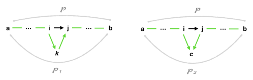
Figure 7: Illustration of paths $\mathcal{P}$, $\mathcal{P}_{1},\mathcal{P}_{2}$.

We first show that $\left(\operatorname{pa}_{\mathcal{G}_{2}}(j)\cap\operatorname{ch}_{\mathcal{G}_{2}}(i)\right)\cap\mathcal{S}\subseteq C\cap\mathcal{S}$. Let $k$ be an arbitrary node in $\left(\operatorname{pa}_{\mathcal{G}_{2}}(j)\cap\operatorname{ch}_{\mathcal{G}_{2}}(i)\right)\cap\mathcal{S}$. If $k\notin C$, then the path $\mathcal{P}_{1}:a-\dots-i\to k\to j-\dots b$ by removing $i\to j$ from $\mathcal{P}$ but connecting $i,j$ using $k$ is active given $C$ in $\mathcal{G}_{2}$. This is because all its colliders are colliders of $\mathcal{P}$ and the additional non-collider $k\notin C$. However, $\mathcal{P}_{1}$ is in $\mathcal{G}_{1}$ as it does not contain $i\to j$; a contradiction. Therefore $k\in C$ and $\left(\operatorname{pa}_{\mathcal{G}_{2}}(j)\cap\operatorname{ch}_{\mathcal{G}_{2}}(i)\right)\cap\mathcal{S}\subseteq C\cap\mathcal{S}$.

We now show that $C\cap\mathcal{S}\subseteq\left(\operatorname{pa}_{\mathcal{G}_{2}}(j)\setminus\{i\}\right)\cap\mathcal{S}$. Suppose there is $c\in C\cap\mathcal{S}$ such that $c\notin\operatorname{pa}_{\mathcal{G}_{2}}(j)\setminus\{i\}$. Since $c\in\mathcal{S}$, it is adjacent to both $i,j$ in $\mathcal{G}_{2}$. Thus $i\rightarrow c\leftarrow j$ by $c\notin\operatorname{pa}_{\mathcal{G}_{2}}(j)\setminus\{i\}$ and $i\in\operatorname{pa}_{\mathcal{G}_{2}}(j)$. Then the path $\mathcal{P}_{2}:a-\dots-i\to c\operatorname{\leftarrow}j-\dots-b$ by removing $i\to j$ from $\mathcal{P}$ and connecting $i,j$ using $i\rightarrow c\leftarrow j$ is active given $C$ in $\mathcal{G}_{2}$ (as all its non-colliders are non-colliders of $\mathcal{P}$ and the additional collider $c\in C$). However, $\mathcal{P}_{2}$ is in $\mathcal{G}_{1}$ as it does not contain $i\to j$; a contradiction. Therefore $C\cap\mathcal{S}\subseteq\left(\operatorname{pa}_{\mathcal{G}_{2}}(j)\setminus\{i\}\right)\cap\mathcal{S}$. ∎

With these results the lower bound in Theorem 1 can be proven as described in Section 4 in the main text.

Appendix C OMITTED PROOFS OF UPPER BOUND

We first explain why the total number of maximal undirected cliques in $[\mathcal{G}]$ cannot exceed $n$. Since the undirected edges in $\mathcal{E}(\mathcal{G})$ correspond to a collection of chordal chain components, it suffices to show that in any chordal graph of size $k$, the number of maximal undirected cliques is at most $k$. This is a well-known result; see for example (Dirac,, 1961).

To show the upper bound in Theorem 2, we only need to prove Proposition 9 and Lemma 10. With these results, Theorem 2 can be obtained as described in Section 5.2 in the main text.

Proposition 9.

If $\mathcal{H}\leq\mathcal{G}$ and $\operatorname{skel}(\mathcal{H})\subsetneq\operatorname{skel}(\mathcal{G})$, then there exists a DAG $\mathcal{H}^{\prime}$ such that $\mathcal{H}\leq\mathcal{H}^{\prime}\leq\mathcal{G}$ and $\mathcal{H}^{\prime}$ is missing one edge in $\mathcal{G}^{\prime}$ for some $\mathcal{G}^{\prime}\in[\mathcal{G}]$.

Proof.

By Theorem 4 in (Chickering,, 2002), there exists a sequence of DAGs $\mathcal{G}_{1},\dots,\mathcal{G}_{k}$ such that

• $\mathcal{H}=\mathcal{G}_{k+1}\leq\mathcal{G}_{k}\leq\dots\leq\mathcal{G}_{1}\leq\mathcal{G}_{0}=\mathcal{G}$;

• For each $i\in\{0,\dots,k+1\}$, $\mathcal{G}_{i+1}$ differs from $\mathcal{G}_{i}$ by either a covered edge flip in $\mathcal{G}_{i}$ or a missing edge from $\mathcal{G}_{i}$.

Note that by Lemma 2 in (Chickering,, 2002), if $\mathcal{G}_{i+1}$ differs from $\mathcal{G}_{i}$ by a covered edge flip, then they are in the same MEC. Let $i$ be the smallest index such that $\mathcal{G}_{i+1}$ is missing an edge from $\mathcal{G}_{i}$. Such an $i$ exists since $\operatorname{skel}(\mathcal{H})\neq\operatorname{skel}(\mathcal{G})$. Then $[\mathcal{G}_{i}]=\cdots=[\mathcal{G}_{0}]=[\mathcal{G}]$. Therefore letting $\mathcal{G}^{\prime}=\mathcal{G}_{i}$ and $\mathcal{H}=\mathcal{G}_{i+1}$ concludes the proof. ∎

Lemma 10.

For any $i$ in $\mathcal{G}^{\prime}\in[\mathcal{G}]$, there is $\operatorname{pa}_{\mathcal{G}^{\prime}}(i)=\operatorname{pa}_{[\mathcal{G}]}(i)\cup C$ for some undirected clique $C\subseteq\operatorname{adj}_{[\mathcal{G}]}(i)$.

Proof.

As reviewed in Section 2.3, all directed edges in the essential graph of $[\mathcal{G}]$ are shared by $\mathcal{G}^{\prime}$. Therefore $\operatorname{pa}_{\mathcal{G}^{\prime}}(i)\subseteq\operatorname{pa}_{[\mathcal{G}]}\cup\operatorname{adj}_{[\mathcal{G}]}(i)$.

We now show that $\operatorname{pa}_{\mathcal{G}^{\prime}}(i)\cap\operatorname{adj}_{[\mathcal{G}]}(i)$ is an undirected clique. For $j\neq k\in\operatorname{pa}_{\mathcal{G}^{\prime}}(i)\cap\operatorname{adj}_{[\mathcal{G}]}(i)$, if $j\not\sim k$ in $[\mathcal{G}]$, then $j\to i\operatorname{\leftarrow}k$ construes a v-structure in $\mathcal{G}^{\prime}$ that is not in $[\mathcal{G}]$; a contradiction to $\mathcal{G}^{\prime}\in[\mathcal{G}]$. Thus $j\sim k$ in $[\mathcal{G}]$. Furthermore $j\sim k$ must be undirected. Otherwise assume $j\to k$ without loss of generality. We have $j\sim i\sim k$ in one undirected chain component of $[\mathcal{G}]$ and $j\sim i$, $i\sim k$ in different maximal cliques. As reviewed in Section 2.3, it follows from Wienöbst et al., (2021) that there is some DAG in $[\mathcal{G}]$ such that the maximal clique containing $i\sim k$ is the most upstream and $k\to i$. This creates a cycle $k\to i\to j\to k$; a contradiction. Therefore $j\sim k$ must be undirected. Thus $\operatorname{pa}_{\mathcal{G}^{\prime}}(i)\cap\operatorname{adj}_{[\mathcal{G}]}(i)$ is an undirected clique. ∎

Appendix D AN EXAMPLE

We give an example of a DAG whose maximum undirected clique size is $2$ but its MEC has size $\exp(\Omega(n))$. Consider the DAG in Figure 8: it starts off with two v-structures and then continues with repeated block structures. In its essential graph, all black edges are directed (from v-structures and Meek rule 1), whereas all green edges are undirected and can be oriented in all possible ways. Therefore its maximum undirected clique size is $2$ but its MEC has size $2^{n/2-1}=\exp(\Omega(n))$.

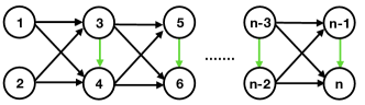
Figure 8: An example DAG.

References

- Acid and de Campos, (2003) Acid, S. and de Campos, L. M. (2003). Searching for bayesian network structures in the space of restricted acyclic partially directed graphs. Journal of Artificial Intelligence Research, 18:445–490.
- Alonso-Barba et al., (2013) Alonso-Barba, J. I., Gámez, J. A., Puerta, J. M., et al. (2013). Scaling up the greedy equivalence search algorithm by constraining the search space of equivalence classes. International journal of approximate reasoning, 54(4):429–451.
- Andersson et al., (1997) Andersson, S. A., Madigan, D., and Perlman, M. D. (1997). A characterization of markov equivalence classes for acyclic digraphs. The Annals of Statistics, 25(2):505–541.
- Andrews et al., (2023) Andrews, B., Ramsey, J., Sanchez Romero, R., Camchong, J., and Kummerfeld, E. (2023). Fast scalable and accurate discovery of dags using the best order score search and grow shrink trees. Advances in Neural Information Processing Systems, 36.
- Batu et al., (2001) Batu, T., Fischer, E., Fortnow, L., Kumar, R., Rubinfeld, R., and White, P. (2001). Testing random variables for independence and identity. In Proceedings 42nd IEEE Symposium on Foundations of Computer Science, pages 442–451. IEEE.
- Batu et al., (2000) Batu, T., Fortnow, L., Rubinfeld, R., Smith, W. D., and White, P. (2000). Testing that distributions are close. In Proceedings 41st Annual Symposium on Foundations of Computer Science, pages 259–269. IEEE.
- Batu et al., (2004) Batu, T., Kumar, R., and Rubinfeld, R. (2004). Sublinear algorithms for testing monotone and unimodal distributions. In Proceedings of the thirty-sixth annual ACM symposium on Theory of computing, pages 381–390.
- Brenner and Sontag, (2013) Brenner, E. and Sontag, D. (2013). Sparsityboost: A new scoring function for learning bayesian network structure. arXiv preprint arXiv:1309.6820.
- Bu et al., (2016) Bu, Y., Zou, S., Liang, Y., and Veeravalli, V. V. (2016). Estimation of kl divergence between large-alphabet distributions. In 2016 IEEE International Symposium on Information Theory (ISIT), pages 1118–1122.
- Canonne, (2020) Canonne, C. L. (2020). A survey on distribution testing: Your data is big. but is it blue? Theory of Computing, pages 1–100.
- Chan et al., (2014) Chan, S.-O., Diakonikolas, I., Valiant, P., and Valiant, G. (2014). Optimal algorithms for testing closeness of discrete distributions. In Proceedings of the twenty-fifth annual ACM-SIAM symposium on Discrete algorithms, pages 1193–1203. SIAM.
- Chickering, (1995) Chickering, D. M. (1995). A transformational characterization of equivalent bayesian network structures. In Proceedings of the Eleventh conference on Uncertainty in artificial intelligence, pages 87–98.
- Chickering, (2002) Chickering, D. M. (2002). Optimal structure identification with greedy search. Journal of machine learning research, 3(Nov):507–554.
- Chickering et al., (2004) Chickering, M., Heckerman, D., and Meek, C. (2004). Large-sample learning of bayesian networks is np-hard. Journal of Machine Learning Research, 5:1287–1330.
- Cho et al., (2016) Cho, H., Berger, B., and Peng, J. (2016). Reconstructing Causal Biological Networks through Active Learning. PLoS ONE, 11(3):e0150611.
- Choo et al., (2023) Choo, D., Gouleakis, T., and Bhattacharyya, A. (2023). Active causal structure learning with advice. In International Conference on Machine Learning, pages 5838–5867. PMLR.
- Claassen et al., (2013) Claassen, T., Mooij, J., and Heskes, T. (2013). Learning sparse causal models is not np-hard. arXiv preprint arXiv:1309.6824.
- Colombo et al., (2011) Colombo, D., Maathuis, M. H., Kalisch, M., and Richardson, T. S. (2011). Learning high-dimensional dags with latent and selection variables. In Proceedings of the Twenty-Seventh Conference on Uncertainty in Artificial Intelligence, pages 850–850.
- Dawid, (1979) Dawid, A. P. (1979). Conditional independence in statistical theory. Journal of the Royal Statistical Society Series B: Statistical Methodology, 41(1):1–15.
- De Campos and Ji, (2011) De Campos, C. P. and Ji, Q. (2011). Efficient Structure Learning of Bayesian Networks using Constraints. The Journal of Machine Learning Research, 12:663–689.
- de Campos et al., (2019) de Campos, L. M., Cano, A., Castellano, J. G., and Moral, S. (2019). Combining gene expression data and prior knowledge for inferring gene regulatory networks via Bayesian networks using structural restrictions. Statistical Applications in Genetics and Molecular Biology, 18(3).
- Dirac, (1961) Dirac, G. A. (1961). On rigid circuit graphs. In Abhandlungen aus dem Mathematischen Seminar der Universität Hamburg, volume 25, pages 71–76. Springer.
- Eberhardt and Scheines, (2007) Eberhardt, F. and Scheines, R. (2007). Interventions and Causal Inference. Philosophy of science, 74(5):981–995.
- Fisher et al., (1943) Fisher, R. A., Corbet, A. S., and Williams, C. B. (1943). The relation between the number of species and the number of individuals in a random sample of an animal population. The Journal of Animal Ecology, pages 42–58.
- Flores et al., (2011) Flores, M. J., Nicholson, A. E., Brunskill, A., Korb, K. B., and Mascaro, S. (2011). Incorporating expert knowledge when learning Bayesian network structure: A medical case study. Artificial intelligence in medicine, 53(3):181–204.
- Friedman et al., (2000) Friedman, N., Linial, M., Nachman, I., and Pe’er, D. (2000). Using bayesian networks to analyze expression data. Journal of computational biology, 7(3-4):601–620.
- Geiger and Heckerman, (2002) Geiger, D. and Heckerman, D. (2002). Parameter priors for directed acyclic graphical models and the characterization of several probability distributions. The Annals of Statistics, 30(5):1412–1440.
- Geiger and Pearl, (1990) Geiger, D. and Pearl, J. (1990). On the logic of causal models. In Machine Intelligence and Pattern Recognition, volume 9, pages 3–14. Elsevier.
- Goldreich et al., (1998) Goldreich, O., Goldwasser, S., and Ron, D. (1998). Property testing and its connection to learning and approximation. Journal of the ACM (JACM), 45(4):653–750.
- Good, (1953) Good, I. J. (1953). The population frequencies of species and the estimation of population parameters. Biometrika, 40(3-4):237–264.
- Hoover, (1990) Hoover, K. D. (1990). The logic of causal inference: Econometrics and the Conditional Analysis of Causation. Economics & Philosophy, 6(2):207–234.
- Indyk et al., (2012) Indyk, P., Levi, R., and Rubinfeld, R. (2012). Approximating and testing k-histogram distributions in sub-linear time. In Proceedings of the 31st ACM SIGMOD-SIGACT-SIGAI symposium on Principles of Database Systems, pages 15–22.
- Jiao et al., (2015) Jiao, J., Venkat, K., Han, Y., and Weissman, T. (2015). Minimax estimation of functionals of discrete distributions. IEEE Transactions on Information Theory, 61(5):2835–2885.
- Kalisch and Bühlman, (2007) Kalisch, M. and Bühlman, P. (2007). Estimating high-dimensional directed acyclic graphs with the pc-algorithm. Journal of Machine Learning Research, 8(3).
- King et al., (2004) King, R. D., Whelan, K. E., Jones, F. M., Reiser, P. G. K., Bryant, C. H., Muggleton, S. H., Kell, D. B., and Oliver, S. G. (2004). Functional genomic hypothesis generation and experimentation by a robot scientist. Nature, 427(6971):247–252.
- Lam et al., (2022) Lam, W.-Y., Andrews, B., and Ramsey, J. (2022). Greedy relaxations of the sparsest permutation algorithm. In Uncertainty in Artificial Intelligence, pages 1052–1062. PMLR.
- Lauritzen, (1996) Lauritzen, S. L. (1996). Graphical models, volume 17. Clarendon Press.
- Li and Beek, (2018) Li, A. and Beek, P. (2018). Bayesian Network Structure Learning with Side Constraints. In International conference on probabilistic graphical models, pages 225–236. PMLR.
- Long et al., (2023) Long, S., Piché, A., Zantedeschi, V., Schuster, T., and Drouin, A. (2023). Causal discovery with language models as imperfect experts. arXiv preprint arXiv:2307.02390.
- McAllester and Schapire, (2000) McAllester, D. A. and Schapire, R. E. (2000). On the convergence rate of good-turing estimators. In COLT, pages 1–6.
- Meek, (1995) Meek, C. (1995). Causal Inference and Causal Explanation with Background Knowledge. In Proceedings of the Eleventh Conference on Uncertainty in Artificial Intelligence, UAI’95, page 403–410, San Francisco, CA, USA. Morgan Kaufmann Publishers Inc.
- Meek, (1997) Meek, C. (1997). Graphical Models: Selecting causal and statistical models. PhD thesis, Carnegie Mellon University.
- Mohammadi et al., (2018) Mohammadi, F., Uhler, C., Wang, C., and Yu, J. (2018). Generalized permutohedra from probabilistic graphical models. SIAM Journal on Discrete Mathematics, 32(1):64–93.
- Nandy et al., (2018) Nandy, P., Hauser, A., and Maathuis, M. H. (2018). High-dimensional consistency in score-based and hybrid structure learning. The Annals of Statistics, 46(6A):3151–3183.
- Orlitsky et al., (2003) Orlitsky, A., Santhanam, N. P., and Zhang, J. (2003). Always good turing: Asymptotically optimal probability estimation. Science, 302(5644):427–431.
- Orlitsky et al., (2016) Orlitsky, A., Suresh, A. T., and Wu, Y. (2016). Optimal prediction of the number of unseen species. Proceedings of the National Academy of Sciences, 113(47):13283–13288.
- Paninski, (2008) Paninski, L. (2008). A coincidence-based test for uniformity given very sparsely sampled discrete data. IEEE Transactions on Information Theory, 54(10):4750–4755.
- Pearl, (1988) Pearl, J. (1988). Probabilistic reasoning in intelligent systems: networks of plausible inference. Morgan kaufmann.
- Pearl, (2003) Pearl, J. (2003). Causality: models, reasoning, and inference. Econometric Theory, 19(4):675–685.
- Pearl, (2009) Pearl, J. (2009). Causal inference in statistics: An overview. Statistics Surveys, 3:96.
- Peters and Bühlmann, (2015) Peters, J. and Bühlmann, P. (2015). Structural intervention distance for evaluating causal graphs. Neural computation, 27(3):771–799.
- Pingault et al., (2018) Pingault, J.-B., O’reilly, P. F., Schoeler, T., Ploubidis, G. B., Rijsdijk, F., and Dudbridge, F. (2018). Using genetic data to strengthen causal inference in observational research. Nature Reviews Genetics, 19(9):566–580.
- Reichenbach, (1956) Reichenbach, H. (1956). The Direction of Time, volume 65. University of California Press.
- Robins et al., (2000) Robins, J. M., Hernan, M. A., and Brumback, B. (2000). Marginal structural models and causal inference in epidemiology. Epidemiology, pages 550–560.
- Rotmensch et al., (2017) Rotmensch, M., Halpern, Y., Tlimat, A., Horng, S., and Sontag, D. (2017). Learning a Health Knowledge Graph from Electronic Medical Records. Scientific reports, 7(1):1–11.
- Rubinfeld and Sudan, (1996) Rubinfeld, R. and Sudan, M. (1996). Robust characterizations of polynomials with applications to program testing. SIAM Journal on Computing, 25(2):252–271.
- Scheines et al., (1998) Scheines, R., Spirtes, P., Glymour, C., Meek, C., and Richardson, T. (1998). he TETAD Project: Constraint Based Aids to Causal Model Specification. Multivariate Behavioral Research, 33(1):65–117.
- Schulte et al., (2010) Schulte, O., Frigo, G., Greiner, R., and Khosravi, H. (2010). The imap hybrid method for learning gaussian bayes nets. In Advances in Artificial Intelligence: 23rd Canadian Conference on Artificial Intelligence, Canadian AI 2010, Ottawa, Canada, May 31–June 2, 2010. Proceedings 23, pages 123–134. Springer.
- Solus et al., (2021) Solus, L., Wang, Y., and Uhler, C. (2021). Consistency guarantees for greedy permutation-based causal inference algorithms. Biometrika, 108(4):795–814.
- Spirtes et al., (1989) Spirtes, P., Glymour, C., and Scheines, R. (1989). Causality from probability.
- Spirtes et al., (2000) Spirtes, P., Glymour, C. N., and Scheines, R. (2000). Causation, prediction, and search. MIT press.
- Spirtes et al., (2013) Spirtes, P. L., Meek, C., and Richardson, T. S. (2013). Causal inference in the presence of latent variables and selection bias. arXiv preprint arXiv:1302.4983.
- Sverchkov and Craven, (2017) Sverchkov, Y. and Craven, M. (2017). A review of active learning approaches to experimental design for uncovering biological networks. PLoS computational biology, 13(6):e1005466.
- Tian, (2016) Tian, T. (2016). Bayesian Computation Methods for Inferring Regulatory Network Models Using Biomedical Data. Translational Biomedical Informatics: A Precision Medicine Perspective, pages 289–307.
- Tsamardinos et al., (2006) Tsamardinos, I., Brown, L. E., and Aliferis, C. F. (2006). The max-min hill-climbing bayesian network structure learning algorithm. Machine learning, 65:31–78.
- Valiant and Valiant, (2011) Valiant, G. and Valiant, P. (2011). Estimating the unseen: An n/log(n)-sample estimator for entropy and support size, shown optimal via new clts. In Proceedings of the Forty-third Annual ACM Symposium on Theory of Computing, STOC ’11, pages 685–694, New York, NY, USA. ACM.
- Valiant and Valiant, (2017) Valiant, G. and Valiant, P. (2017). An automatic inequality prover and instance optimal identity testing. SIAM Journal on Computing, 46(1):429–455.
- Vashishtha et al., (2023) Vashishtha, A., Reddy, A. G., Kumar, A., Bachu, S., Balasubramanian, V. N., and Sharma, A. (2023). Causal inference using llm-guided discovery. arXiv preprint arXiv:2310.15117.
- Verma and Pearl, (1990) Verma, T. and Pearl, J. (1990). Equivalence and synthesis of causal models. In Proceedings of the Sixth Annual Conference on Uncertainty in Artificial Intelligence, pages 255–270.
- Wienöbst et al., (2021) Wienöbst, M., Bannach, M., and Liskiewicz, M. (2021). Polynomial-time algorithms for counting and sampling markov equivalent dags. In Proceedings of the AAAI Conference on Artificial Intelligence, volume 35, pages 12198–12206.
- Woodward, (2005) Woodward, J. (2005). Making Things Happen: A Theory of Causal Explanation. Oxford University Press.
- Wu and Yang, (2015) Wu, Y. and Yang, P. (2015). Chebyshev polynomials, moment matching, and optimal estimation of the unseen. ArXiv e-prints, arXiv:1504.01227.