Hybrid Quantum-inspired Resnet and Densenet for Pattern Recognition with Completeness Analysis

Abstract

With the contemporary digital technology approaching, deep neural networks are emerging as the foundational algorithm of the artificial intelligence boom. Whereas, the evolving social demands have been emphasizing the necessity of novel methodologies to substitute traditional neural networks. Concurrently, the advent of the post-Moore era has spurred the development of quantum-inspired neural networks with outstanding potentials at certain circumstances. Nonetheless, a definitive evaluating system with detailed metrics is tremendously vital and indispensable owing to the vague indicators in comparison between the novel and traditional deep learning models at present. Hence, to improve and evaluate the performances of the novel neural networks more comprehensively in complex and unpredictable environments, we propose two hybrid quantum-inspired neural networks which are rooted in residual and dense connections respectively for pattern recognitions with completeness representation theory for model assessment. Comparative analyses against pure classical models with detailed frameworks reveal that our hybrid models with lower parameter complexity not only match the generalization power of pure classical models, but also outperform them notably in resistance to parameter attacks with various asymmetric noises. Moreover, our hybrid models indicate unique superiority to prevent gradient explosion problems through theoretical argumentation. Eventually, We elaborate on the application scenarios where our hybrid models are applicable and efficient, which paves the way for their industrialization and commercialization.

I Introduction

As the cornerstone of AI technology, deep neural network algorithms have played a pivotal role in varied applications over the past few decades, owing to their remarkable learning capacities to comprehend complicated patterns [2, 3, 4, 5, 6, 7, 8, 9, 10, 11, 12, 13, 14, 15, 16, 17, 18, 19, 20]. Nevertheless, in light of the rapid pace of industrialization and commercialization, it remains a formidable challenge for deep neural networks to adequately satisfy the multifaceted demands of societal advancements. One of the most significant primary concerns lies in the inherent trade-off between generalization power, robustness and complexity [21, 22, 23, 24, 25]. Traditional deep neural networks with low complexity often struggle to generalize well and exhibit vulnerability to adversarial attacks, while neural networks with relatively stronger generalization power and robustness are resource-intensive [21, 22, 23]. Fortunately, the arrival of post-Moore era has catalyzed the advancement of quantum computing, particularly quantum neural networks [26]. Innovative frameworks involve quantum stochastic neural networks, soft quantum neural computing paradigms, and variational circuit models [26, 27, 28, 29]. Furthermore, there has been another burgeoning computing paradigm, quantum-inspired neural network, which obeys partial rules of quantum computing and all the regulations of deep learning [30, 31, 32]. On the basis of quantum neural networks, quantum-inspired neural networks also possess the capability to break through the bottleneck of pure classical neural networks on account of their prominent performances on certain circumstances and a small amount of resource consumption with the algorithms disposed on authentic quantum computer [31, 33]. However, the inherent unpredictability and dynamism of industrial and commercial domains necessitate the novel models to consistently exhibit commensurate capabilities with or surpass pure classical models on more miscellaneous environments, especially with diverse noisy and noiseless datasets, as well as assorted parameter attacks [34, 35, 36, 37]. More crucially, as for the comparison between the novel and traditional models, the nebulous assessing indicators and the evaluation criteria lead to weak interpretability of the advantages of quantum-inspired networks under complicated scenarios [5, 8, 33]. Therefore, how to ameliorate the universality of the novel models to substitute traditional ones under clear standards has become a hotspot in deep learning methodologies [2].

Hence, to expand the scope of the quantum-inspired networks, there is strong anticipation for the emergence of quantum-inspired neural network algorithms with hybrid forms, which are grounded on different strengths of pure classical and quantum-inspired algorithms [26, 38, 39, 40, 41]. It represents the amalgamation of pure classical parts and quantum-inspired parts [41]. Owing to a paucity of works in the exploration on this intricate framework, we firstly design novel hybrid Quantum-inspired Residual and Dense Feedforward Neural Network models (QRFNN,QDFNN) and hybrid Quantum-inspired Residual and Dense Convolutional Neural Network models (QRCNN,QDCNN). The models are inspired by Resnet, Densenet and optical circuit models and applied in pattern recognition problems, which is predicated on our interest [42, 43, 44]. The residual and dense connections facilitate feature propagation in the hidden layers, which thereby minimizes feature degradation and enhances model adaptability [42, 43]. Simultaneously, optical circuits unveils unprecedented potential to save computing resources because of the characteristics of quantum bits if the hybrid models are deployed on actual quantum computers for execution[44]. Moreover, to showcase the holistic prowess of our models, we introduce the representation completeness theory for deep neural networks in classification tasks, which is supplemented by relevant indicators [2]. Classical Multi-Layer Perceptron (MLP) and Convolutional Neural Networks (CNN) with detailed structures serve as benchmarks for model comparisons with the completeness theory. With regard to the myriad hyperparameters, we center predominantly on delineating the architectures and behaviors of our hybrid and pure classical models, while ensuring the hyperparameters to be almost the same (see supplementary materials part F). We sincerely hope our work will herald a future where hybrid quantum-inspired architectures redefine the boundaries of deep learning and propel AI technology to unprecedented heights. Contributions originating from the paper are:

• designing and analysing hybrid QRFNN and QDFNN models for iris data recognition [45] under noisy and noiseless environments on classical computers;

• designing and analysing hybrid QRCNN and QDCNN models for MNIST, FASHIONMNIST and CIFAR100 image classification [45] under noisy and noiseless environments on classical computers;

• proposing representation completeness theory of deep neural network on recognition issues, which contains generalization power, robustness, complexity, intepretability and convergence;

• comparing the hybrid and pure classical structures according to the completeness theory in detail, discussing the advantages of our hybrid models and analysing the corresponding reasons of the advantages;

• illustrating the application scenerios of the hybrid frameworks.

Next, in section 2, we review the corresponding works of classical residual and dense learning frameworks, as well as quantum deep learning which is represented by circuit models. In section 3, we introduce some basic concepts of circuit models, Resnet and Densenet. We explain our hybrid models in accordance with the completeness theory thoroughly in section 4. Following it, many groups of numerical simulations on both hybrid and pure classical models are provided in section 5. Finally, we conclude the results and give the future work in section 6.

II Related Work

II-A Circuit learning models

Circuit model can be regarded as a quantum deep learning paradigm with backpropogation to update parameters for feature learning [46, 47]. In the real quantum circuit system, classical data is encoded into quantum states initially, then the features are acquired via evolutionary processes which concern quantum gates, finally the processes culminate in the extraction of the classical information from the quantum states through measurement. In previous studies, the unitary gates include ${\rm R}_{\rm Y},{\rm R}_{\rm Z}$, Hadamard and CNOT gates, some of which contain no parameter but just change the dimensional indices of the vector spaces where the parameters exist [26, 46, 47]. Therefore, to enable the models to fully extract the features, all the logic gates are designed with sparse matrices, each of which are imbued with a parameter. The symmetrical ”V” shape in Fig. 3 assures sufficient quantity of parameters for feature storages of each category in the datasets [17]. And the evolutionary process also conforms to the sparse coding mechanism of visual cells during the human visual perception process [48, 49]. Acknowledging the considerable duration entailed by measurements, we opt to ignore measurement operations in the quantum-inspired frameworks. What’s more, leveraging the insights gleaned from completeness theoretical analysis, we elucidate the disparities between pure classical and hybrid network structures, which thus fortifies our methodologies with enhanced theoretical substantiation.

II-B Resnet and Densenet

In spite of the proposal of deep neural networks due to the obstacles to shallow neural networks in accommodating extensive information from datasets with high-dimensional features [2, 3], simulation findings have also underscored the impediments in training traditional deep neural networks, especially feature disappearance [42, 43]. Consequently, in 2016, Resnet, which features skip connections, and Densenet, which employs feature concatenation, were introduced, and showcased remarkable accuracy in image classification [42, 43]. The two architectures achieve the advantages of the element-wise addition mechanism and the feature map concatenation mechanism. Besides the remarkable effects in mitigating feature vanishing, the approaches also shows a heightened capacity to overcome gradient vanishing [42, 43]. Large-scale deep neural networks for practical problems, such as YOLO in autonomous driving and attention-based Transformer in text translation, draw inspiration specifically from these seminal works [11, 14]. With the absence of prior research on hybrid quantum-inspired Resnet and Densenet with circuit models, we embark on pioneering efforts to devise both frameworks. On the basis of the element-wise addition mechanism to minimize information loss, these frameworks represent an innovative leap forward in deep learning architectures.

III Preliminary

III-A Qubits and circuit models

Analogous to classical bit for information storage in electronic computer, a qubit is the unit in quantum algorithms, which is described as a 2-dimensional complex vector in Hilbert space in algebra and expressed by Dirac notations. It can be written from the superposition rules:

$$\ket{\psi}=\alpha\ket{0}+\beta\ket{1},\enspace|\alpha|^{2}+|\beta|^{2}=1\;(\alpha,\beta\in\mathbb{C}).$$ (1)

In the avant-garde framework, the evolution process stands for the manipulation to the quantum states by continuous unitary operations [46]:

$$\ket{\psi_{m}}=U_{m}\ket{\psi_{m-1}}\quad(m\in\mathbb{N}^{+}),$$ (2)

where $U$ represents unitary quantum gates, $m$ denotes the number of the evolutions. When $m$ = 1, $\rm{\ket{\psi_{0}}}$ means the initial state. And the gate utilized in the paper is the $T$ gate:

$$\scriptsize T_{i,i+1}(\theta^{l}_{r})=\pNiceMatrix[first-col,last-row]&10\cdots\cdots\cdots\cdots\cdots 0\\ 01\vdots\\ \vdots\ddots\vdots\\ i\vdots\cos({\mathrm{\theta}}^{l}_{r}){\rm-sin}(\theta^{l}_{r})\vdots\\ i+1\vdots\sin({\rm\theta}^{l}_{r})\cos({\rm\theta}^{l}_{r})\vdots\\ \vdots\ddots\vdots\\ \vdots 10\\ 0\cdots\cdots\cdots\cdots\cdots 01\\ ii+1\\$$ (3)

where $l$ denotes the layer index $(l\in\mathbb{N})$, $i$ denotes the row index of ${\rm-sin}({\theta}^{l}_{r})$ and the column index of $\sin({\theta}^{l}_{r})$ $(i\in\mathbb{N}^{+})$. And $r$ means the parameter index $(r\in\mathbb{N})$.

III-B Resnet and Densenet learning

Realizing the noise in the preceding layers with interference to the feature spaces [2], we propose linear additions with adaptive parameters $\lambda$ to reduce miscellaneous noise impacts. In terms of the Resnet, Fig. 1 shows its first two-layer structure. And $H_{h}(x)=R_{h-1}(H_{h-1}(x))\oplus\lambda_{h-1}H_{h-1}(x)(h\in\mathbb{N}^{+})$, where $\oplus$ means linear element-wise addition, $R_{h-1}$ is described as residual mappings of the $h^{th}$ layer. In Densenet, the initial version is derived from the feature map concatenation [43]. To simplify it for adaptation to our issues, our version emanates from the element-wise addition with linear dense connection of all the preceding layers in Fig. 2, where $G_{a}(x)=D_{a-1}(G_{a-1}(x))\oplus\lambda_{a,0}x\oplus\sum\limits^{a-1}_{b=1}\lambda_{{a,b}}G_{b}(x)(a,b\in\mathbb{N}^{+})$ for more layers, where $D_{a-1}$ refers to dense mappings of the $a^{th}$ layer.

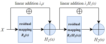
Figure 1: Residual connection of Resnet.

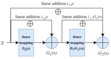
Figure 2: Dense connection of Densenet.

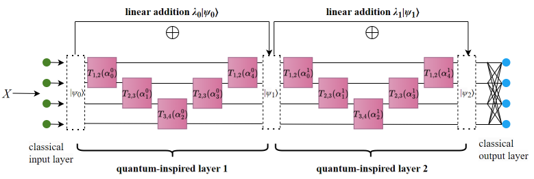
(a)

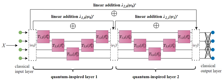
(b)

Figure 3: QRFNN and QDFNN. (a) QRFNN. (b) QDFNN.

IV Hybrid models with completeness analysis

We delineate the hybrid models with specific architectures, which include model interpretability and complexity.

IV-A Intepretability

IV-A1 Layer details

Interpretability refers to the ability to provide explanations in understandable terms [2]. Firstly we analyse the structure details of layers. Fig. 3 demonstrates the QRFNN and QDFNN structures of 2 qubits with 2 layers, where every line represents one-dimensional vector space of a quantum state. The green, blue circles denote the input and output neurons respectively. We also build the quantum-inspired layers as hidden layers in QRFNN and QDFNN rather than classical hidden layers with neurons. Considering one sample in an iteration and setting there are $n$ lines and $N$ qubits $(2^{N-1}<n\leq 2^{N})$, which also alludes to the $n$ dimensions of the input, $X=(x_{1},x_{2},...,x_{n})^{\top}$, for every layer, we define:

$$U_{l}=\prod\limits_{\begin{subarray}{c}i=0\end{subarray}}^{\begin{subarray}{c}i=n-2\end{subarray}}[T_{i+1,i+2}(\theta_{i}^{l})]\times\prod\limits_{\begin{subarray}{c}i=n-1\end{subarray}}^{\begin{subarray}{c}i=2n-4\end{subarray}}[T_{2n-3-i,2n-2-i}(\theta_{i}^{l})]\quad(l\in\mathbb{N}),$$ (4a)

$$U_{l}^{\prime}=\prod\limits_{\begin{subarray}{c}i=0\end{subarray}}^{\begin{subarray}{c}i=n-2\end{subarray}}[T_{i+1,i+2}(\beta_{i}^{l})]\times\prod\limits_{\begin{subarray}{c}i=n-1\end{subarray}}^{\begin{subarray}{c}i=2n-4\end{subarray}}[T_{2n-3-i,2n-2-i}(\beta_{i}^{l})]\quad(l\in\mathbb{N}),$$ (4b)

where $U_{l},U_{l}^{\prime}$ are the unitary matrices of QRFNN and QDFNN seperately, and the parameter index is also represented with $i$. Accordingly, $n$-dimensional inputs correspond with $2n-3$ parameters in one hidden layer for feature storage and transfer. Suppose there are both $L$ quantum-inspired layers and $L+2$ layers totally in the two models. Firstly, we encode the inputs into the amplitude of the state in the input layers of the two models:

$$\ket{\psi_{0}}=\sum\limits_{\begin{subarray}{c}d=1,k=0\end{subarray}}^{\begin{subarray}{c}d=n,k=n-1\end{subarray}}\frac{x_{d}}{\sqrt{{\sum^{n}_{d=1}}x_{d}^{2}}}\ket{k},$$ (5)

where $k=\sum\limits^{n}_{e=1}p_{e}\cdot 2^{n-e}$, and $p_{e}$ denotes the binary representation. Secondly, in terms of QRFNN:

$$\ket{\psi_{l}}=U_{l-1}\ket{\psi_{l-1}}\oplus\lambda_{l-1}\ket{\psi_{l-1}}\quad(1\leq l\leq L).$$ (6)

While for QDFNN:

$$\ket{\psi_{l}}^{\prime}=U_{l-1}^{\prime}\ket{\psi_{l-1}}^{\prime}\oplus\sum^{i=l-1}_{i=0}\lambda_{l,i}\ket{\psi_{i}}^{\prime}\quad(1\leq l\leq L).$$ (7)

Next, $\ket{\psi_{L}},\ket{\psi_{L}}^{\prime}$ are the outputs of the last quantum-inspired layers of QRFNN and QDFNN, which are represented as classical column vectors $O_{L},O_{L}^{\prime}$ now (see supplementary materials part A). $O_{L}=(o_{L,1},o_{L,2},...,o_{L,n})^{\top},O_{L}^{\prime}=(o_{L,1}^{\prime},o_{L,2}^{\prime},...,o_{L,n}^{\prime})^{\top}$, where $o_{L,j},o_{L,j}^{\prime}$ denote the output at the $j^{th}$ dimensional index of the last hidden layer. Eventually, for both QRFNN and QDFNN, with $O_{L},O_{L}^{\prime}$ transmitted into the classical output layer, the final output will be:

$$O_{L+1}=s((W_{L+1}\cdot O_{L})^{\top}+B_{L+1}),$$ (8a)

$$O_{L+1}^{\prime}=s((W_{L+1}^{\prime}\cdot O_{L}^{\prime})^{\top}+B_{L+1}^{\prime}),$$ (8b)

where $s$ denotes softmax activation, $W_{L+1}$ and $W_{L+1}^{\prime}$ mean the weight matrices of the output layers of QRFNN and QDFNN seperately, while $B_{L+1},B_{L+1}^{\prime}$ represent biases, the row vectors of the output layers of QRFNN and QDFNN respectively. Nevertheless, aware of the limited input types that the two models can handle, we try adding convolutional parts with residual connection modules in front of QRFNN and with dense connection modules in front of QDFNN to keep the model frameworks highly consistent for image recognition. Relying on the previous work [50], we design QDCNN and QRCNN, where the residual and dense blocks are both composed of the channel and spatial attentions in parallel to improve time efficiency (see Fig. 4). And the two attention operations are concatenated in channel index, which is described as the Orange-yellow oval in Fig. 4. For both QDCNN and QRCNN, given a feature map $F\in\mathbb{R}^{C\times H\times W}$ as input, we firstly do a traditional convolutional operation with $3\times 3$ kernel gaining feature maps $F_{1}$ and $F_{1}^{\prime}$. Then they are operated with the paralleled attentions in the residual and dense blocks separately. Channel attention, $A_{c}$, consists of a shared MLP for different levels of importance to different channels [50]. Spatial attention, $A_{s}$, is constituted by pooling, convolution, and concatenation operation for distinct significance levels of elements in different positions of a feature map [50]. These two attentions are pivotal in the extraction of localized features. Furthermore, for the output feature map of the $(g-1)^{th}$ layer, also the input feature map of the $g^{th}$ layer in the residual block of QRCNN, $F_{g}$:

$$F_{g}=c(A_{c}(F_{g-1}),A_{s}(F_{g-1}))\boxplus f^{1\times 1}(F_{g-1})\quad(g\geq 2).$$ (9)

When it comes to the output feature map of the $(g-1)^{th}$ layer, also the input feature map of the $g^{th}$ layer in the dense block of QDCNN, $F_{g}^{\prime}$:

$$F_{g}^{\prime} =c(A_{c}(F_{g-1}^{\prime}),A_{s}(F_{g-1}^{\prime}))\boxplus E_{g},$$ (10a)

$$E_{g} =f^{1\times 1}(F_{1}^{\prime})\boxplus f^{1\times 1}(F_{2}^{\prime})\boxplus...\boxplus f^{1\times 1}(F_{g-1}^{\prime})\quad(g\geq 2),$$ (10b)

where $c$ is the concatenation operation of the feature maps in channel index. $f$ stands for the convolutional operation. $\boxplus$ denotes the element-wise addition between the feature maps after the concatenation or convolution operations, which is also expressed as the blue square in Fig. 4. $E_{g}$ means the element-wise additions of all the input feature maps in the preceding $g-1$ layers in the dense block, from $F_{1}^{\prime}$ to $F_{g-1}^{\prime}$. The $1\times 1$ convolution operations in Eq. (9) and (10b) serve to increase the dimension of the input feature map in channel index in each preceding layer to be the same to facilitate the element-wise addition, which promotes feature incorporation as well. With $F_{g}$ and $F_{g}^{\prime}$ convolved and flattened eventually, QRFNN and QDFNN are linked after the convolutional parts of QRCNN and QDCNN respectively.

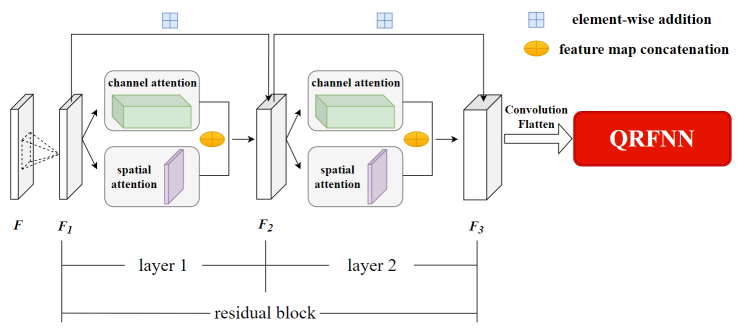
(a)

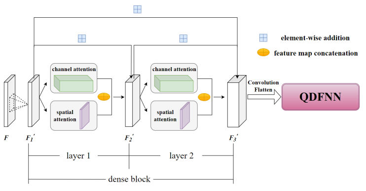
(b)

Figure 4: QRCNN and QDCNN. (a) QRCNN. (b) QDCNN. With respect to the two convolutional parts of QRCNN and QDCNN, both of them are comprised of attention layers in the residual or dense block and traditional convolutional layers. And the ”layer” in the figure means the attention layers in the residual or dense block, which are our focus.

IV-A2 Model transparency

To contrast the transparency of the pure classical and hybrid models, we take the positions where the parameters are located within the models into account. Suppose there is an MLP with $K$ layers totally, where there are $M_{S}$ neurons in the $S^{th}$ layer $(1\leq S\leq K)$. And the output vector of the $S^{th}$ layer is $O_{S}^{\prime\prime}$. Suppose the output of a sample is of the $j^{th}$ dimensional index of the output layer (see supplementary materials part A for more model details), we have:

$$o_{L,j} =\sum^{n}_{j=1}h_{j}\cdot o_{L-1,j},$$ (11a)

$$o_{L,j}^{\prime} =\sum^{n}_{j=1}h_{j}^{\prime}\cdot o_{L-1,j}^{\prime},$$ (11b)

$$o_{K,q}^{\prime\prime} =\sigma(\sum\limits_{u=1}^{M_{K-1}}\sum\limits_{q=1}^{M_{k}}w_{u,q}^{\prime\prime}\cdot o_{K-1,u}^{\prime\prime}+b_{q}^{\prime\prime}).$$ (11c)

When it comes to QRFNN and QDFNN in Eq. (11a) and (11b), $h_{j}$ denotes the linear summations of the multiplications of the basic terms, $\lambda_{h},\sin(\theta^{l}_{r}),\cos(\theta^{l}_{r})(0\leq h\leq L-1,0\leq l\leq L-1,0\leq r\leq 2n-4)$ of QRFNN, which means the parameters with different parameter and layer indices are multiplied together for feature transfer. Identically, $h_{j}^{\prime}$ is also expressed as that of the basic terms, $\lambda_{a,b},\sin(\beta^{l}_{r}),\cos(\beta^{l}_{r})(1\leq a\leq L,0\leq b\leq L-1,0\leq l\leq L-1,0\leq r\leq 2n-4)$ of QDFNN. And with respect to Eq. (11c), $o_{K,q}^{\prime\prime}$ denotes the output of the $q^{th}$ dimensional index of the output layer of the MLP. $O_{K}^{\prime\prime}=(o_{K,1}^{\prime\prime},o_{K,2}^{\prime\prime},...,o_{K,M_{K}}^{\prime\prime})$, where $O_{K}^{\prime\prime}$ represents the output vector of the ${K}^{th}$ layer in the MLP. $o_{K-1,u}^{\prime\prime}$ is the output of the $u^{th}$ dimensional index of the ${(K-1)}^{th}$ layer. And $\sigma$ is any kind of activation, $w_{u,q}^{\prime\prime}$ is the weight between the $u^{th}$ neuron node in the ${(K-1)}^{th}$ layer and the $q^{th}$ neuron node in the ${K}^{th}$ layer, which belongs to the ${K}^{th}$ layer. $b_{q}^{\prime\prime}$ represents the bias in the $q^{th}$ neuron node in the ${K}^{th}$ layer. The similarity of the three models lies in the feedforward layer-by-layer transfer of features by parameters in the hidden layers. Each parameter in the hidden layers participate in the predicted outputs of all the samples with varied categories. However, if we regard the last quantum-inspired layers as the output layers in QRFNN and QDFNN temporarily, and we concentrate on the parameters of the output layers of QRFNN, QDFNN, and the MLP, only a few of weights and biases contribute to the predicted output of each sample in the MLP, while almost all the parameters of the output layers involve in the predicted output of each sample in our hybrid models without the classical output layers. In addition, for QRFNN and QDFNN, to compute the derivative of a certain $\theta_{r}^{l}$ of the $r^{th}$ parameter index in the $l^{th}$ layer to update all the parameters in the models, we just require acquisition of the derivative matrix of $T_{i,i+1}(\theta^{l}_{r})$, that is $Z_{i,i+1}(\theta^{l}_{r})$:

$$\scriptsize=\pNiceMatrix[first-col,last-row]&10\cdots\cdots\cdots\cdots\cdots 0\\ 01\vdots\\ \vdots\ddots\vdots\\ i\vdots\frac{{\rm d(cos}(\theta^{l}_{r}))}{{\rm d}\theta^{l}_{r}}\frac{{\rm d(-sin}(\theta^{l}_{r}))}{{\rm d}\theta^{l}_{r}}\vdots\\ i+1\vdots\frac{{\rm d(sin}(\theta^{l}_{r}))}{{\rm d}\theta^{l}_{r}}\frac{{\rm d(cos}(\theta^{l}_{r}))}{{\rm d}\theta^{l}_{r}}\vdots\\ \vdots\ddots\vdots\\ \vdots 10\\ 0\cdots\cdots\cdots\cdots\cdots 01\\ ii+1\\$$

$$\scriptsize=\pNiceMatrix[first-col,last-row]&10\cdots\cdots\cdots\cdots\cdots 0\\ 01\vdots\\ \vdots\ddots\vdots\\ i\vdots{\rm-sin}(\theta^{l}_{r}){\rm-cos}(\theta^{l}_{r})\vdots\\ i+1\vdots\cos(\theta^{l}_{r}){\rm-sin}(\theta^{l}_{r})\vdots\\ \vdots\ddots\vdots\\ \vdots 10\\ 0\cdots\cdots\cdots\cdots\cdots 01\\ ii+1\\$$ (12)

Now in regard to the backpropagation of QRFNN and QDFNN, we contemplate both the classical output layer and the quantum-inspired hidden layers. Conscious of the gradient of $O_{l}$ and $O_{l}^{\prime}$, to the $r^{th}$ parameter in the $l^{th}$ quantum-inspired layer, $\theta_{r}^{l}$ $(0\leq r\leq 2n-4,1\leq l\leq L)$, and taking the predicted outputs from samples with different categories into consideration, we derive that:

$$\frac{\partial O_{l}}{\partial\theta_{r}^{l}} =\prod\limits_{j=0}^{r-1}T(\theta_{j}^{l})\cdot Z(\theta_{r}^{l})\cdot\prod\limits_{j=r+1}^{2n-4}T(\theta_{j}^{l})\cdot O_{l-1},$$ (13a)

$$\frac{\partial O_{l}^{\prime}}{\partial\beta_{r}^{l}} =\prod\limits_{j=0}^{r-1}T(\beta_{j}^{l})\cdot Z(\beta_{r}^{l})\cdot\prod\limits_{j=r+1}^{2n-4}T(\beta_{j}^{l})\cdot O_{l-1}^{\prime}.$$ (13b)

To simplify the representations, we omit the subscripts for $T$ and $Z$. We also deduce that:

$$\frac{\partial(loss)}{\partial\theta_{r}^{l}} =\frac{\partial(loss)}{\partial O_{L+1}}\cdot\prod\limits_{j=l}^{L}\frac{\partial O_{L+l+1-j}}{\partial O_{L+l-j}}\cdot\frac{\partial O_{l}}{\partial\theta_{r}^{l}},$$ (14a)

$$\frac{\partial(loss^{\prime})}{\partial\beta_{r}^{l}} =\frac{\partial(loss^{\prime})}{\partial O_{L+1}^{\prime}}\cdot\prod\limits_{j=l}^{L}\frac{\partial O_{L+l+1-j}^{\prime}}{\partial O_{L+l-j}^{\prime}}\cdot\frac{\partial O_{l}^{\prime}}{\partial\beta_{r}^{l}},$$ (14b)

where $loss$ and $loss^{\prime}$ denote the loss functions of QRFNN and QDFNN seperately. While $\frac{\partial(loss)}{\partial O_{L+1}}$ and $\frac{\partial O_{L+1}}{\partial O_{L}}$ follow the derivative rules of pure classical neural networks with weights and biases [3], for most quantum-inspired layers, we deduce the gradient matrix of $\frac{\partial O_{l}}{\partial O_{l-1}}(1<l\leq L)$:

$$\nabla_{l,l-1}=\large\begin{pmatrix}\frac{\partial o_{l,1}}{\partial o_{l-1,1}}&\frac{\partial o_{l,2}}{\partial o_{l-1,1}}&\cdots&\cdots&\frac{\partial o_{l,n}}{\partial o_{l-1,1}}\\[9.0pt] \frac{\partial o_{l,1}}{\partial o_{l-1,2}}&\frac{\partial o_{l,2}}{\partial o_{l-1,2}}&\cdots&\cdots&\frac{\partial o_{l,n}}{\partial o_{l-1,2}}\\[9.0pt] \vdots&\vdots&\ddots&&\vdots\\[9.0pt] \vdots&\vdots&&\ddots&\frac{\partial o_{l,n}}{\partial o_{l-1,n-1}}\\[9.0pt] \frac{\partial o_{l,1}}{\partial o_{l-1,n}}&\frac{\partial o_{l,2}}{\partial o_{l-1,n}}&\cdots&\frac{\partial o_{l,n-1}}{\partial o_{l-1,n}}&\frac{\partial o_{l,n}}{\partial o_{l-1,n}}\\[9.0pt] \end{pmatrix}$$ (15)

And the gradient matrix of $\frac{\partial O_{l}^{\prime}}{\partial O_{l-1}^{\prime}}(1<l\leq L)$ is:

$$\nabla_{l,l-1}^{\prime}=\large\begin{pmatrix}\frac{\partial o_{l,1}^{\prime}}{\partial o_{l-1,1}^{\prime}}&\frac{\partial o_{l,2}^{\prime}}{\partial o_{l-1,1}^{\prime}}&\cdots&\cdots&\frac{\partial o_{l,n}^{\prime}}{\partial o_{l-1,1}^{\prime}}\\[9.0pt] \frac{\partial o_{l,1}^{\prime}}{\partial o_{l-1,2}^{\prime}}&\frac{\partial o_{l,2}^{\prime}}{\partial o_{l-1,2}^{\prime}}&\cdots&\cdots&\frac{\partial o_{l,n}^{\prime}}{\partial o_{l-1,2}^{\prime}}\\[9.0pt] \vdots&\vdots&\ddots&&\vdots\\[9.0pt] \vdots&\vdots&&\ddots&\frac{\partial o_{l,n}^{\prime}}{\partial o_{l-1,n-1}^{\prime}}\\[9.0pt] \frac{\partial o_{l,1}^{\prime}}{\partial o_{l-1,n}^{\prime}}&\frac{\partial o_{l,2}^{\prime}}{\partial o_{l-1,n}^{\prime}}&\cdots&\frac{\partial o_{l,n-1}^{\prime}}{\partial o_{l-1,n}^{\prime}}&\frac{\partial o_{l,n}^{\prime}}{\partial o_{l-1,n}^{\prime}}\\[9.0pt] \end{pmatrix}$$ (16)

In accordance with Eq. (3), (4a), (4b), (6) and (7), with regard to each $\frac{\partial o_{l,v}}{\partial o_{l-1,w}}(1\leq v\leq n,1\leq w\leq n,2\leq l\leq L,v,w\in\mathbb{N}^{+})$, it is the linear summations of the multiplications of the basic terms in the $l^{th}$ layer, $\sin(\theta_{y}^{l-1}),\cos(\theta_{y}^{l-1}),\lambda_{l-1}(0\leq y\leq 2n-4)$. And each $\frac{\partial o_{l,v}^{\prime}}{\partial o_{l-1,w}^{\prime}}$ also stands for the linear summations of the multiplications of the fundamental components in the $l^{th}$ layer, $\sin(\beta_{y}^{l-1}),\cos(\beta_{y}^{l-1}),\lambda_{l,i}(0\leq i\leq l-1)$. Therefore, the gradient computations are also composed of the additions and multiplications of $\lambda_{l-1}$, $\lambda_{l,i}$, sine and cosine functions of varied layers predominantly. Some groups of simulations in section 5 suggest the brilliant ability of our hybrid models to prevent gradient explosion effectively. The reason is that the ranges of sine and cosine functions are both $\rm{[-1,1]}$, thus the stabilities of the gradients of all the terms are ensured in the backpropagation process. Compared with the gradient clipping and regularization methods that can only control the gradient stability to a certain extent [4], our hybrid models demonstrate superior capacities for the issue in a more systematical manner. Additionally, the classical output layer with activations and biases further enhances the ability for nonlinear problems, and adapts to varied data categories. To raise the consistency between the quantum-inspired frameworks and authentic quantum systems, the incorporation of activations in the quantum-inspired layers is eschewed. Nonetheless, there is a cogent rationale to activate the quantum-inspired layers with varied activations [2, 3]. Additionally, with the convenience of altering the number of neuron nodes of the MLP hidden layers leveraged, adding a small quantity of classical hidden layers subsequent to the input layer can achieve high adaptability to input with manifold dimensions in actual situations. Meanwhile, integrating the quantum-inspired layer as the core of the hidden layers in the hybrid models ensures robust security measures (see section 5).

IV-B Complexity

The complexity of neural networks stems from their diverse linking ways between the hidden layers, designs of loss function, the need for effective hyperparameter tuning and so on. On the whole, it is divided into two parts [2, 25]. One part is computational complexity $C$ which depends on the floating operation numbers of the forward procedure computation $C_{f}$, the backpropagation procedure of gradient update $C_{b}$, and the parameter update procedure $C_{w}$. The other is parameter complexity $P$ which is founded on the parameters that are temporarily stored in each epoch $P_{t}$ and stored throughout the training and testing processes $P_{s}$. Since convolutional part is not the most significant in the paper, we only pay attention to the complexity comparison between the hybrid feedforward models and the MLP based on the dynamic programming mechanism. For the MLP, set the floating operation numbers of the activation at the $S^{th}$ layer is $G_{M_{s}}$, and that of the activation derivative at the $S^{th}$ layer is $G_{M_{s}}^{\prime}$. And we utilize the same Momentum Gradient Descent method (MGD) with a regularization term in all the models, of which we set the number of floating operations of each parameter to be $C_{mgd}$. Since testing process has no backpropagation, computational complexity of training process predominates in the computational complexity of MLP, $C_{MLP}$, as well as that of QRFNN and QDFNN, $C_{QRFNN}$ and $C_{QDFNN}$. As for QRFNN and QDFNN, we suppose the dimension of the classical output layer is also $d$-dimensional. We select one epoch with $I$ iterations and batchsize $B$ in each iteration in training as the example. With regard to $C$ of the MLP, we deduce that:

$$C_{f_{1}} =O(\sum^{K}_{s=2}(B\cdot I\cdot G_{M_{s}}\cdot M_{s-1}\cdot M_{s}))+O(\sum^{K}_{s=2}(B\cdot I\cdot G_{M_{s}}\cdot M_{s}))$$

$$=O(\sum^{K}_{s=2}(M_{s-1}+1+G_{M_{s}})B\cdot I\cdot M_{s})$$

$$\approx O(\sum^{K}_{s=2}BIM_{s-1}M_{s}),$$ (17a)

$$C_{b_{1}} =O(\sum^{K}_{s=2}(B\cdot I\cdot G_{M_{s}}^{\prime}\cdot M_{s-1}\cdot M_{s}))+O(\sum^{K}_{s=2}(B\cdot I\cdot G_{M_{s}}^{{}^{\prime}}\cdot M_{s}))$$

$$\approx O(\sum^{K}_{s=2}BIM_{s-1}M_{s}),$$ (17b)

$$C_{w_{1}} =O(\sum^{K}_{s=2}I\cdot C_{mgd}\cdot M_{s-1}\cdot M_{s}+I\cdot M_{s})$$

$$\approx O(\sum^{K}_{s=2}I\cdot M_{s-1}\cdot M_{s}),$$ (17c)

$$C_{MLP} =C_{f_{1}}+C_{b_{1}}+C_{w_{1}}$$

$$\approx O(\sum^{K}_{s=2}BIM_{s-1}M_{s}).$$ (17d)

In terms of $P$ of the MLP, we derive that:

$$P_{t_{1}} =O(\sum^{K}_{s=2}M_{s-1}M_{s})+O(\sum^{K}_{s=3}M_{s-1}M_{s})+O(\sum^{K}_{s=2}M_{s})$$

$$+O(\sum^{K}_{s=3}M_{s})$$

$$\approx O(\sum^{K}_{s=2}M_{s-1}M_{s}),$$ (18a)

$$P_{s_{1}} =O(\sum^{K}_{s=2}M_{s-1}M_{s})+O(\sum^{K}_{s=2}M_{s})$$

$$\approx O(\sum^{K}_{s=2}M_{s-1}M_{s}),$$ (18b)

$$P_{MLP} =P_{t_{1}}+P_{s_{1}}$$

$$\approx O(\sum^{K}_{s=2}M_{s-1}M_{s}).$$ (18c)

For QRFNN, we have:

$$C_{f_{2}} =O(B\cdot I\cdot L\cdot n^{4}+2B\cdot I\cdot(L-1)\cdot n)$$

$$\approx O(BILn^{4}),$$ (19a)

$$C_{b_{2}} =O(B\cdot I\cdot L\cdot n^{4}+2B\cdot I\cdot(L-1)\cdot n)$$

$$\approx O(BILn^{4}),$$ (19b)

$$C_{w_{2}} =O(I\cdot C_{mgd}\cdot(2n-3)),$$

$$\approx O(nIC_{mgd})$$ (19c)

$$C_{QRFNN} =C_{f_{2}}+C_{b_{2}}+C_{w_{2}}$$

$$\approx O(BILn^{4}).$$ (19d)

$$P_{t_{2}} =O(L\cdot(2n-3))+O(L\cdot(2n-4))+O(L-1)$$

$$+O(L-2)+O(nd)+O(d)$$

$$\approx O(nL+nd),$$ (19e)

$$P_{s_{2}} =O(L\cdot(2n-3)+O(nd)+O(d))$$

$$\approx O(nL+nd),$$ (19f)

$$P_{QRFNN} =P_{t_{2}}+P_{s_{2}}$$

$$\approx O(nL+nd).$$

For QDFNN, we have:

$$C_{f_{3}} =O(B\cdot I\cdot L\cdot n^{4}+2B\cdot I\cdot(L-1)^{2}\cdot n)$$

$$\approx O(BILn^{4}),$$ (20a)

$$C_{b_{3}} =O(B\cdot I\cdot L\cdot n^{4}+2B\cdot I\cdot(L-1)^{2}\cdot n)$$

$$\approx O(BILn^{4}),$$ (20b)

$$C_{w_{3}} =O(I\cdot C_{mgd}\cdot(2n-3)),$$ (20c)

$$\approx O(nIC_{mgd})$$ (20d)

$$C_{QDFNN} =C_{f_{3}}+C_{b_{3}}+C_{w_{3}}$$

$$\approx O(BILn^{4}).$$ (20e)

$$P_{t_{3}} =O(L\cdot(2n-3))+O(L\cdot(2n-4))+O(\frac{L(L+1)}{2})$$

$$+O(\frac{L(L+1)}{2}-1)+O(nd)+O(d)$$

$$\approx O(nL+nd),$$ (20f)

$$P_{s_{3}} =O(L\cdot(2n-3))+O(nd)+O(d)$$

$$\approx O(nL+nd),$$ (20g)

$$P_{QDFNN} =P_{t_{3}}+P_{s_{3}}$$

$$\approx O(nL+nd).$$ (20h)

Due to the modest scales of QDFNN and QRFNN, a plenty of indicators and terms in the formulae can not be neglected, thus, we meticulously contemplate numerous indicators of the complexity in our paper. We scrupulously compare the complexities of pure classical and the hybrid models under the precondition that all of the models manifest extraordinary performances without overfitting and underfitting problems. For a more explicit comparison, we make an effort to ensure one of the complexities of the three models to be similar. Owing to the complicated factors of the computational complexity, we try to assure $C_{MLP}$, $C_{QRFNN}$, $C_{QDFNN}$ to be similar for convenience of our research (See supplementary materials part F). And in our hybrid models, $C_{w_{1}}>C_{w_{2}}\approx C_{w_{3}}$, while $C_{f_{1}}<C_{f_{2}}\approx C_{f_{3}}$, and $C_{b_{1}}<C_{b_{2}}\approx C_{b_{3}}$. Under this condition, $P_{t_{1}}>P_{t_{2}}\approx P_{t_{3}},P_{s_{1}}>P_{s_{2}}\approx P_{s_{3}},P_{QRFNN}\approx P_{QDFNN}<P_{MLP}$, which demonstrates the testament to the lightweight of the hybrid feedforward and convolutional models with distinguished behaviors.

V Numerical simulations

We illustrate the strong generalization power and robustness of the four hybrid models with different datasets to ensure the universality in this section. We utilize iris data with three categories for QRFNN and QDFNN. And we choose partial enhanced MNIST, FASHIONMNIST CIFAR100 image datasets with each dataset consisting of four categories for QDCNN and QRCNN.

V-A Generalization power test

Generalization power is appraised by accurancy, precision, recall and f1 score under the condition of the noiseless and noisy dataset testings. To emulate real-world scenarios more faithfully, we select pure Gaussian noises, pure uniform noises and their mixed forms with symmetrical and asymmetric distributions, a total of six cases [36, 37, 51]. The symmetrical noise refers to the symmetrical noise distributions with respect to the y-axis in a Cartesian coordinate system (see supplementary materials part H). To add more uncertainties, the amount and the location of the noise added to the data are random.

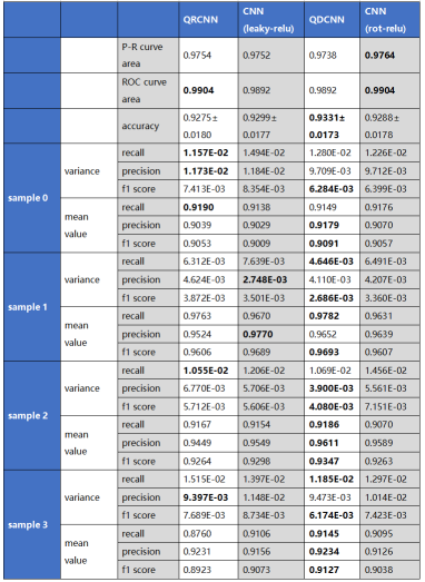
Figure 5: Results with mixed asymmetric noise in FASHIONMNIST dataset. We utilize two pure classical CNNs for comparison with the hybrid models, one of which is activated by leaky-relu function. And the activation function in the other pure classical CNN is rot-relu (see supplementary materials part B).

Fig. 5 demonstrates the recognition outcomes with FASHIONMNIST dataset with mixed asymmetric noise utilized (more results in supplementary materials part C), which include the variances and mean values of many indicators of the four kinds of categories, from sample 0 to sample 3. With successive training until the $100^{th}$ epoch, the loss function exhibits a discernible decline, while the accuracy implys a corresponding increase, after which both metrics level off (an example shown in supplementary materials part E). To justify the stability of all the models after convergence, all the values in the charts are the averages from the $100^{th}$ epoch to the $300^{th}$ epoch (the same in supplementary materials part C), among which lower variances represent higher stability, while higher mean values portend better prediction performances. While precision is concerned with the proportion of the real positive samples out of all the samples that are predicted to be positive, recall is absorbed in the proportion of the real positive samples that are correctly predicted [2]. For an overall evaluation of the models, we utilize ROC, P-R curve area for the imbalance of the number of different categories [2, 5]. The overall outcomes demonstrate that our hybrid quantum-inspired networks with lower parameter complexity perform on par with the two pure classical neural networks in these metrics. For instance, in terms of $\mu^{1}$, the average test accuracies of QRCNN, QDCNN, and the two classical CNNs in FASHIONMNIST with mixed asymmetric noise, $\mu^{1}_{QRCNN}$ = 92.75%, $\mu^{1}_{QDCNN}$ = 93.31%, $\mu^{1}_{CNN(leaky-relu)}$ = 92.99%, and $\mu^{1}_{CNN(rot-relu)}$ = 92.88%.

V-B Robustness test

Robustness is appraised by the same metrics in generalization power part under parameter attacks in miscellaneous environments during training and testing. Contemplating the strong resistance of the large scale convolutional parts in QDCNN and QRCNN [2, 51], we randomly choose a fully-connected layer of the pure classical MLP and CNNs and a quantum-inspired layer of the four hybrid models for attacking. We attack some parameters randomly in those layers with the most likely two forms: ① $g(\theta+\epsilon)$ ② $g(\theta)+\epsilon$, where $\theta$, $\epsilon$ denote parameters and noises respectively. $g$ represents activation operations in pure classical models, while it means sine or cosine functions in the hybrid models [21, 22].

The test of robustness is seperated into symmetrical noise attack with form ① and ② and unsymmetrical noise attack with form ① and ② (see supplementary materials part D for more results). For symmetrical attack, with CIFAR100 dataset, all the models indicate illustrious outcomes on the same level under the premise of lower parameter complexity of the four hybrid models, as shown in Fig. 6. More importantly, the hybrid models reveal more irreplaceable superiority powerfully under unsymmetrical noise attacks in the two forms in Fig. 7 and 8 (see supplementary materials part D for more results). For example, as for $\mu^{2}$, the average test accuracies of QRCNN, QDCNN, and the two classical CNNs in CIFAR100 with uniform asymmetric noise attack, while $\mu^{2}_{CNN(leaky-relu)}$ = 29.95%, and $\mu^{2}_{CNN(rot-relu)}$ = 29.88%, $\mu^{2}_{QRCNN}$ = 75.13%, $\mu^{2}_{QDCNN}$ = 76.74%. With the results of the pure classical models centered on, two occasions are that when the loss function rises to the order of millions, the accuracy curves oscillate badly with the prediction effects to be extremely unstable. And as the loss function reaches NaN, the accuracies are maintained at a low value and the models fail to learn, which originates from gradient explosion. It also suggests the exceptional merits of our hybrid models to avoid gradient explosion.

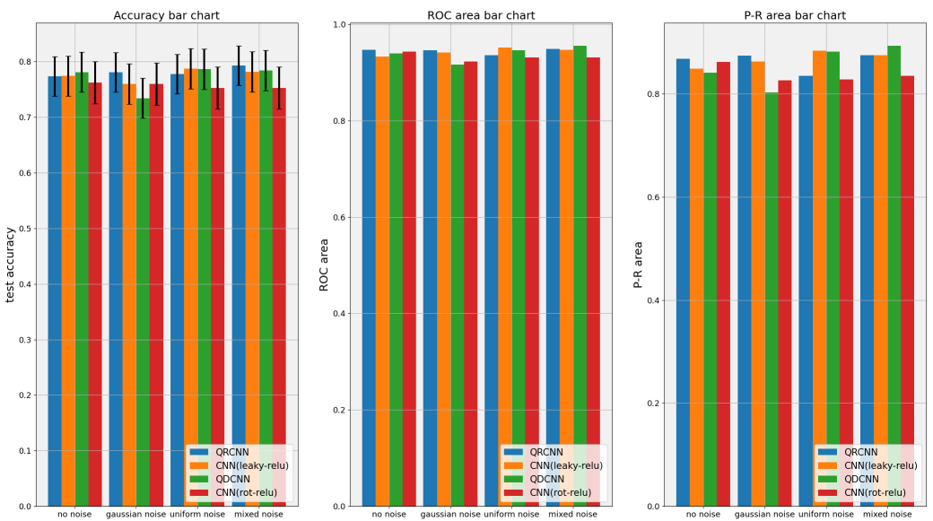
(a)

Figure 6: Accuracy, ROC, P-R curve area bar chart of CIFAR100 with symmetrical noise attack in form ①. We utilize two pure classical CNNs for comparison with the hybrid models, one of which is activated by leaky-relu function. And the activation function in the other pure classical CNN is rot-relu. With respect to the results, both the hybrid models and the pure classical models demonstrate performances on the same level. All the results are the averages from the $100^{th}$ epoch to the $300^{th}$ epoch after convergence (the same in supplementary materials part D).

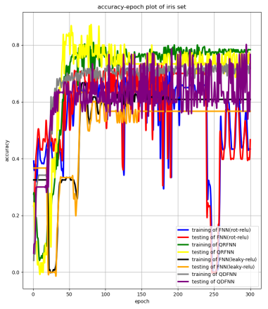
(a)

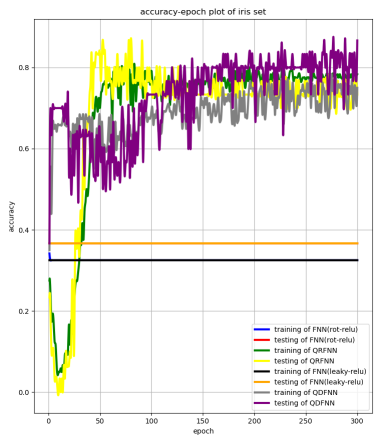
(b)

Figure 7: Unsymmetrical noise attack in form ② in iris. We utilize two pure classical feedforward neural networks (FNN, which denotes MLP here) for comparison with the hybrid models, one of which is activated by leaky-relu function. And the activation function in the other pure classical FNN is rot-relu. (a) Parameter attack with gaussian unsymmetrical noise. (b) Parameter attack with mixed unsymmetrical noise. In respect of the average test accuracies of the two pure classical models, the curve fluctuates badly in (a), while the results remain low values in (b) since the loss reach NaN.

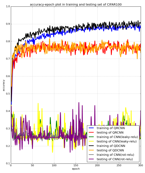
(a)

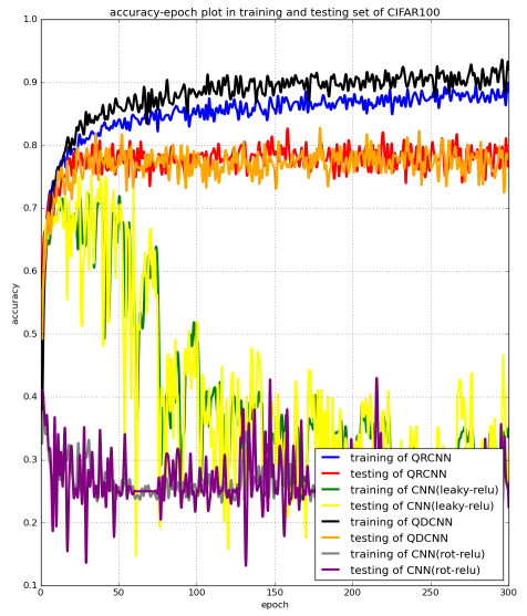
(b)

Figure 8: Unsymmetrical noise attack in form ① in CIFAR100. We utilize two pure classical CNNs for comparison with the hybrid models, one of which is activated by leaky-relu function. And the activation function in the other pure classical CNN is rot-relu.(a) Parameter attack with uniform unsymmetrical noise. (b) Parameter attack with gaussian unsymmetrical noise. When it comes to the average test accuracies of the two pure classical models, the curve fluctuates badly in both (a) and (b).

VI Conclusion and discussion

To summarize, in the paper, we have firstly proposed four hybrid quantum-inspired neural networks with the illustration of their interpretability and complexity, as well as the assessment of their generalization capacity and robustness. Pure classical MLP and CNNs with concrete structures are utilized for comparison in all the classification problems. All the metrics constitute the cornerstone of the completeness theory. In particular, the charm of our hybrid models lies in these dominances:

• They show the same levels of generalization ability and robustness as the pure classical models on the two occasions when the datasets contain the six noises or no noise, and the parameters are attacked by the symmetrical noises;

• They manifest much more unrivalled and outstanding robustness than pure classical models with the parameters attacked by the unsymmetrical noises;

• With the computational complexity to be similar, the parameter complexity of the hybrid models are far lower than that of the pure classical models, which indicates the lightweight if they are deployed on industrial devices;

• On the basis of the algebraic properties of the sine and cosine functions, it raises great potential to systematically prevent the gradient explosion problem during training and testing;

• In the long run, with quantum computers being developed, it is impressive to deploy the models with circuit frameworks on a real quantum device, which will take advantages of higher parallelism and save more computing resources.

Accordingly, all the merits endow them with the status as a nascent neural network architecture, which is poised to supplant traditional MLP and CNN models and thereby heralds a transformative shift in computational efficacy and representational capabilities.

What’s more, noticing the complicated industrial and commercial environments, we discuss the specific application scenarios of the hybrid models. Typically, a natural dataset is perceived as a probability distribution which is delineated upon a manifold space. Samples are regarded as points, a multitude of which constitute a dense point cloud to represent the data feature in the original data space [52]. In view of the natural laws, the distribution of the point clouds on the data manifold space satisfies specific distribution principles [52]. Consequently, the dimensionality and dimension of the feature space are comparatively diminutive in relation to the original manifold data space, which also elucidates the extraordinary outcomes of our hybrid models with fewer parameters and modest hidden-layer spaces. Additionally, the number of layers of a feedforward neural network corresponds to the depth of the network, while the number of neurons or qubits in each layer are defined as the width of the network [53]. On account of the enhanced gradient coherences of the loss function, both deep and wide neural networks imply extraordinary generalization capabilities [51]. Nonetheless, whether the neural networks with different structures are capable of performing well is also determined by the dimension of the feature space of the input data, $W_{in}$, and the optimization methods [54]. Assume that the dimension of the hidden layer space of a deep neural network is $W_{hid}$. Generally, when $W_{hid}\geq W_{in}$, cooperating with appropriate activations, the deep neural networks usually show more extraordinary approximation effects. When $W_{hid}<W_{in}$, wider neural networks will harness their stroger strengths over the deep networks for the problem owing to the information loss caused by the discrepancy of $W_{hid}$ and $W_{in}$ [53, 54, 55]. According to Eq. (19d) and (20e), $C_{QRFNN}\propto L,C_{QRFNN}\propto n^{4}\propto 2^{4N},C_{QDFNN}\propto L,C_{QDFNN}\propto n^{4}\propto 2^{4N}$, which indicates the trouble to expand the width and the feasibility to improve the depth of our hybrid models. Therefore, they exhibit greater aptness for data whose feature spaces are of moderate scales.

Based on this article, there are still some points for further development. For instance, how to ensure the distinguished behaviors of the hybrid frameworks under the condition of expanding the model width for the dimension increase of features will be a direction worth thinking about. Furthermore, broadening the application ranges of our hybrid models to address more profound AI challenges, such as text-based image generation, or integrating them with robotics, has the potential to precipitate substantial societal revolution. We honestly look forward to the leap from the laboratory to practical applications of our hybrid models.

Click here for supplementary material information

Biography Section

Andi Chen received the B.S. degree from Dalian University of Technology and University of Leicester with joint cultivation mechanism in 2022. Now he is a postgraduate whose major is brain science and artificial intelligence in Brain Science and Artificial Intelligent Institute for Brain Sciences and Kuang Yaming Honors School in Nanjing University and Hefei National Laboratory in University of Science and Technology of China. He is the exchange student studying assistive robotic systems of National Yang Ming Chiao Tung University of Taiwan. His research interest includes novel deep learning algorithms for science, reinforcement learning for assistive robotic systems and multimodal generative learning systems.

Hua-Lei Yin received the B.S. degree from University of Science and Technology of China in 2012, and the Ph.D. degree in quantum information physics from the same university in 2016. He had been an associate professor of School of Physics at Nanjing University since 2019. Now he is an associate professor of the Department of Physics and Beijing Key Laboratory of Opto-Electronic Functional Materials and Micro-Nano Devices, Key Laboratory of Quantum State Construction and Manipulation (Ministry of Education), Renmin University of China. His research interest includes cryptography, information theory, quantum communication science, and quantum artificial intelligence algorithms.

Zeng-Bing Chen received the B.S. degree and Ph.D. degree from University of Science and Technology of China in 1995 and 2000, respectively. He became a professor at University of Science and Technology of China in 2004 and he has been a professor at Nanjing University since 2018. His research interest includes the fundamental problems of quantum theory, quantum information theory, information theory and quantum-inspired artificial intelligence algorithms.

Shengjun Wu received the B.S. degree from the University of Science and Technology of China in 1997 and the Ph.D. degree from the University of South Carolina in 2003. He is currently a professor in the School of Physics at Nanjing University and the Hefei National Laboratory at the University of Science and Technology of China. His current research focuses on quantum information science, foundations of quantum mechanics, and quantum artificial intelligence.

References

- [1] Y. LeCun, Y. Bengio, and G. Hinton, “Deep learning,” nature, vol. 521, no. 7553, pp. 436–444, 2015.
- [2] I. Goodfellow, Y. Bengio, and A. Courville, Deep learning. MIT press, 2016.
- [3] S. J. Prince, Understanding Deep Learning. MIT press, 2023.
- [4] J. Schmidhuber, “Deep learning in neural networks: An overview,” Neural networks, vol. 61, pp. 85–117, 2015.
- [5] L. Deng, D. Yu et al., “Deep learning: methods and applications,” Foundations and trends® in signal processing, vol. 7, no. 3–4, pp. 197–387, 2014.
- [6] Y. Guo, Y. Liu, A. Oerlemans, S. Lao, S. Wu, and M. S. Lew, “Deep learning for visual understanding: A review,” Neurocomputing, vol. 187, pp. 27–48, 2016.
- [7] J. Ngiam, A. Khosla, M. Kim, J. Nam, H. Lee, and A. Y. Ng, “Multimodal deep learning,” in Proceedings of the 28th international conference on machine learning (ICML-11), 2011, pp. 689–696.
- [8] I. A. Basheer and M. Hajmeer, “Artificial neural networks: fundamentals, computing, design, and application,” Journal of microbiological methods, vol. 43, no. 1, pp. 3–31, 2000.
- [9] S. B. Laughlin and T. J. Sejnowski, “Communication in neuronal networks,” Science, vol. 301, no. 5641, pp. 1870–1874, 2003.
- [10] R. Girshick, “Fast r-cnn,” in Proceedings of the IEEE international conference on computer vision, 2015, pp. 1440–1448.
- [11] Q. Chen, Y. Wang, T. Yang, X. Zhang, J. Cheng, and J. Sun, “You only look one-level feature,” in Proceedings of the IEEE/CVF conference on computer vision and pattern recognition, 2021, pp. 13 039–13 048.
- [12] Y. Lin, I. Koprinska, and M. Rana, “Ssdnet: State space decomposition neural network for time series forecasting,” in 2021 IEEE International Conference on Data Mining (ICDM). IEEE, 2021, pp. 370–378.
- [13] H. Zhao, J. Shi, X. Qi, X. Wang, and J. Jia, “Pyramid scene parsing network,” in Proceedings of the IEEE conference on computer vision and pattern recognition, 2017, pp. 2881–2890.
- [14] A. Vaswani, N. Shazeer, N. Parmar, J. Uszkoreit, L. Jones, A. N. Gomez, Ł. Kaiser, and I. Polosukhin, “Attention is all you need,” Advances in neural information processing systems, vol. 30, 2017.
- [15] J. Deng, W. Dong, R. Socher, L.-J. Li, K. Li, and L. Fei-Fei, “Imagenet: A large-scale hierarchical image database,” in 2009 IEEE conference on computer vision and pattern recognition. Ieee, 2009, pp. 248–255.
- [16] O. Ronneberger, P. Fischer, and T. Brox, “U-net: Convolutional networks for biomedical image segmentation,” in Medical Image Computing and Computer-Assisted Intervention–MICCAI 2015: 18th International Conference, Munich, Germany, October 5-9, 2015, Proceedings, Part III 18. Springer, 2015, pp. 234–241.
- [17] F. Milletari, N. Navab, and S.-A. Ahmadi, “V-net: Fully convolutional neural networks for volumetric medical image segmentation,” in 2016 fourth international conference on 3D vision (3DV). Ieee, 2016, pp. 565–571.
- [18] S. Minaee, Y. Boykov, F. Porikli, A. Plaza, N. Kehtarnavaz, and D. Terzopoulos, “Image segmentation using deep learning: A survey,” IEEE transactions on pattern analysis and machine intelligence, vol. 44, no. 7, pp. 3523–3542, 2021.
- [19] A. Hering, L. Hansen, T. C. Mok, A. C. Chung, H. Siebert, S. Häger, A. Lange, S. Kuckertz, S. Heldmann, W. Shao et al., “Learn2reg: comprehensive multi-task medical image registration challenge, dataset and evaluation in the era of deep learning,” IEEE Transactions on Medical Imaging, vol. 42, no. 3, pp. 697–712, 2022.
- [20] Z. Li, F. Liu, W. Yang, S. Peng, and J. Zhou, “A survey of convolutional neural networks: analysis, applications, and prospects,” IEEE transactions on neural networks and learning systems, 2021.
- [21] Y. Shen and J. Wang, “Robustness analysis of global exponential stability of recurrent neural networks in the presence of time delays and random disturbances,” IEEE transactions on neural networks and learning systems, vol. 23, no. 1, pp. 87–96, 2011.
- [22] J. Wang, A. Pal, Q. Yang, K. Kant, K. Zhu, and S. Guo, “Collaborative machine learning: Schemes, robustness, and privacy,” IEEE Transactions on Neural Networks and Learning Systems, 2022.
- [23] K. Zhou, Z. Liu, Y. Qiao, T. Xiang, and C. C. Loy, “Domain generalization: A survey,” IEEE Transactions on Pattern Analysis and Machine Intelligence, 2022.
- [24] P. R. Bassi, S. S. Dertkigil, and A. Cavalli, “Improving deep neural network generalization and robustness to background bias via layer-wise relevance propagation optimization,” Nature Communications, vol. 15, no. 1, p. 291, 2024.
- [25] A. R. Muotri and F. H. Gage, “Generation of neuronal variability and complexity,” Nature, vol. 441, no. 7097, pp. 1087–1093, 2006.
- [26] K. Beer, D. Bondarenko, T. Farrelly, T. J. Osborne, R. Salzmann, D. Scheiermann, and R. Wolf, “Training deep quantum neural networks,” Nature communications, vol. 11, no. 1, p. 808, 2020.
- [27] L.-J. Wang, J.-Y. Lin, and S. Wu, “Implementation of quantum stochastic walks for function approximation, two-dimensional data classification, and sequence classification,” Physical Review Research, vol. 4, no. 2, p. 023058, 2022.
- [28] J.-Y. Lin, X.-Y. Li, Y.-H. Shao, W. Wang, and S. Wu, “Implementing arbitrary quantum operations via quantum walks on a cycle graph,” Physical Review A, vol. 107, no. 4, p. 042405, 2023.
- [29] M.-G. Zhou, Z.-P. Liu, H.-L. Yin, C.-L. Li, T.-K. Xu, and Z.-B. Chen, “Quantum neural network for quantum neural computing,” Research, vol. 6, p. 0134, 2023.
- [30] D. Szwarcman, D. Civitarese, and M. Vellasco, “Quantum-inspired neural architecture search,” in 2019 International Joint Conference on Neural Networks (IJCNN). IEEE, 2019, pp. 1–8.
- [31] P. J. Coles, “Seeking quantum advantage for neural networks,” Nature Computational Science, vol. 1, no. 6, pp. 389–390, 2021.
- [32] W. Ye, R. Liu, Y. Li, and L. Jiao, “Quantum-inspired evolutionary algorithm for convolutional neural networks architecture search,” in 2020 IEEE Congress on Evolutionary Computation (CEC). IEEE, 2020, pp. 1–8.
- [33] S. Song, Y. Hou, and G. Liu, “The interpretability of quantum-inspired neural network,” in 2021 4th International Conference on Artificial Intelligence and Big Data (ICAIBD). IEEE, 2021, pp. 294–298.
- [34] B. Kosko, K. Audhkhasi, and O. Osoba, “Noise can speed backpropagation learning and deep bidirectional pretraining,” Neural Networks, vol. 129, pp. 359–384, 2020.
- [35] N. Semenova, L. Larger, and D. Brunner, “Understanding and mitigating noise in trained deep neural networks,” Neural Networks, vol. 146, pp. 151–160, 2022.
- [36] Y. Xiao, M. Adegok, C.-S. Leung, and K. W. Leung, “Robust noise-aware algorithm for randomized neural network and its convergence properties,” Neural Networks, p. 106202, 2024.
- [37] D. F. Nettleton, A. Orriols-Puig, and A. Fornells, “A study of the effect of different types of noise on the precision of supervised learning techniques,” Artificial intelligence review, vol. 33, pp. 275–306, 2010.
- [38] Y. Liang, W. Peng, Z.-J. Zheng, O. Silvén, and G. Zhao, “A hybrid quantum–classical neural network with deep residual learning,” Neural Networks, vol. 143, pp. 133–147, 2021.
- [39] N. Schetakis, D. Aghamalyan, P. Griffin, and M. Boguslavsky, “Review of some existing qml frameworks and novel hybrid classical–quantum neural networks realising binary classification for the noisy datasets,” Scientific Reports, vol. 12, no. 1, p. 11927, 2022.
- [40] D. Konar, A. D. Sarma, S. Bhandary, S. Bhattacharyya, A. Cangi, and V. Aggarwal, “A shallow hybrid classical–quantum spiking feedforward neural network for noise-robust image classification,” Applied Soft Computing, vol. 136, p. 110099, 2023.
- [41] P. Li, H. Xiao, F. Shang, X. Tong, X. Li, and M. Cao, “A hybrid quantum-inspired neural networks with sequence inputs,” Neurocomputing, vol. 117, pp. 81–90, 2013.
- [42] K. He, X. Zhang, S. Ren, and J. Sun, “Deep residual learning for image recognition,” in Proceedings of the IEEE conference on computer vision and pattern recognition, 2016, pp. 770–778.
- [43] G. Huang, Z. Liu, L. Van Der Maaten, and K. Q. Weinberger, “Densely connected convolutional networks,” in Proceedings of the IEEE conference on computer vision and pattern recognition, 2017, pp. 4700–4708.
- [44] W. R. Clements, P. C. Humphreys, B. J. Metcalf, W. S. Kolthammer, and I. A. Walmsley, “Optimal design for universal multiport interferometers,” Optica, vol. 3, no. 12, pp. 1460–1465, 2016.
- [45] F. Pedregosa, G. Varoquaux, A. Gramfort, V. Michel, B. Thirion, O. Grisel, M. Blondel, P. Prettenhofer, R. Weiss, V. Dubourg et al., “Scikit-learn: Machine learning in python,” the Journal of machine Learning research, vol. 12, pp. 2825–2830, 2011.
- [46] K. Mitarai, M. Negoro, M. Kitagawa, and K. Fujii, “Quantum circuit learning,” Physical Review A, vol. 98, no. 3, p. 032309, 2018.
- [47] G. Chiribella, G. M. D’Ariano, and P. Perinotti, “Quantum circuit architecture,” Physical review letters, vol. 101, no. 6, p. 060401, 2008.
- [48] B. A. Olshausen and D. J. Field, “Emergence of simple-cell receptive field properties by learning a sparse code for natural images,” Nature, vol. 381, no. 6583, pp. 607–609, 1996.
- [49] W. E. Vinje and J. L. Gallant, “Sparse coding and decorrelation in primary visual cortex during natural vision,” Science, vol. 287, no. 5456, pp. 1273–1276, 2000.
- [50] S. Woo, J. Park, J.-Y. Lee, and I. S. Kweon, “Cbam: Convolutional block attention module,” in Proceedings of the European conference on computer vision (ECCV), 2018, pp. 3–19.
- [51] S. Chatterjee and P. Zielinski, “On the generalization mystery in deep learning,” arXiv preprint arXiv:2203.10036, 2022.
- [52] T. Lin and H. Zha, “Riemannian manifold learning,” IEEE transactions on pattern analysis and machine intelligence, vol. 30, no. 5, pp. 796–809, 2008.
- [53] I. Safran and O. Shamir, “Depth-width tradeoffs in approximating natural functions with neural networks,” in Proceedings of the 34th International Conference on Machine Learning, ser. Proceedings of Machine Learning Research, D. Precup and Y. W. Teh, Eds., vol. 70. PMLR, 06–11 Aug 2017, pp. 2979–2987. [Online]. Available: https://proceedings.mlr.press/v70/safran17a.html
- [54] Z. Lu, H. Pu, F. Wang, Z. Hu, and L. Wang, “The expressive power of neural networks: A view from the width,” Advances in neural information processing systems, vol. 30, 2017.
- [55] R. Eldan and O. Shamir, “The power of depth for feedforward neural networks,” in 29th Annual Conference on Learning Theory, ser. Proceedings of Machine Learning Research, V. Feldman, A. Rakhlin, and O. Shamir, Eds., vol. 49. Columbia University, New York, New York, USA: PMLR, 23–26 Jun 2016, pp. 907–940. [Online]. Available: https://proceedings.mlr.press/v49/eldan16.html