Bounding Stochastic Safety: Leveraging Freedman’s Inequality with Discrete-Time Control Barrier Functions

Abstract

When deployed in the real world, safe control methods must be robust to unstructured uncertainties such as modeling error and external disturbances. Typical robust safety methods achieve their guarantees by always assuming that the worst-case disturbance will occur. In contrast, this paper utilizes Freedman’s inequality in the context of discrete-time control barrier functions (DTCBFs) and c-martingales to provide stronger (less conservative) safety guarantees for stochastic systems. Our approach accounts for the underlying disturbance distribution instead of relying exclusively on its worst-case bound and does not require the barrier function to be upper-bounded, which makes the resulting safety probability bounds more directly useful for intuitive safety constraints such as signed distance. We compare our results with existing safety guarantees, such as input-to-state safety (ISSf) and martingale results that rely on Ville’s inequality. When the assumptions for all methods hold, we provide a range of parameters for which our guarantee is stronger. Finally, we present simulation examples, including a bipedal walking robot, that demonstrate the utility and tightness of our safety guarantee.

I Introduction

Safety—typically characterized as the forward-invariance of a safe set [1]—has become a popular area of study within control theory, with broad applications to autonomous vehicles, medical and assistive robotics, aerospace systems, and beyond. Ensuring safety for these systems requires one to account for unpredictable, real-world effects. Ideally, controllers should be designed to ensure robust safety which degrades smoothly with increasing uncertainty. Historically, control theory has treated the problem of safety under uncertainty using deterministic methods, often seeking safety guarantees in the presence of bounded disturbances. This problem has been studied using a variety of safe control approaches including control barrier functions (CBFs) [2], backwards Hamilton-Jacobi (HJ) reachability [3], and state-constrained model-predictive control (MPC) [4]. However, this worst-case analysis often leads to conservative performance since it ensures robustness to adversarial disturbances which are uncommon in practice.

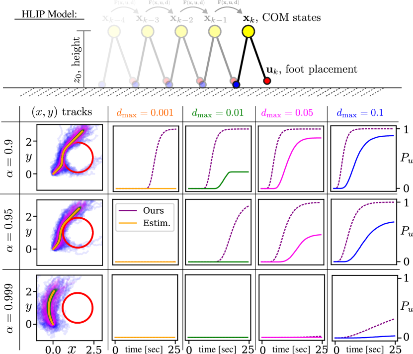
Figure 1: Safety results for a bipedal robot navigating around an obstacle using our method. Details are provided in Section IV. (Top) Visualization of the Hybrid Linear Inverted Pendulum (HLIP) model. Yellow indicates the center-of-mass (COM), blue is the stance foot, and red is the swing foot. The states $\mathbf{x}_{k}$ are the global COM position, the relative COM position, and COM velocity, and the input is the relative position of the feet at impact. This model gives us an approximate discrete-time model for walking. (Bottom) A table with variable maximum disturbance value $(d_{\textup{max}})$ and controller parameter ($\alpha$) shows our theoretical bound on safety failure from Thm. 3 as a dotted line and approximated probabilities from 5000 trials as solid colored lines (lower is better). On the left, the trajectories of the COM are shown from above with each color corresponding to a different $d_{\textup{max}}$. The robot attempts to avoid the obstacle (red). Code to reproduce this plot can be found at [5].

Stochastic methods provide an alternative to the worst-case bounding approach. Instead of a conservative over-approximation of uncertainty’s effect on safety, these methods consider the entire distribution of possible disturbances. Although they do not provide the absolute, risk-free safety guarantees of the worst-case bounding methods, they allow for smooth degradation of safety via variable, risk-aware levels of conservatism. Some authors have provided strong probabilistic safety guarantees for stochastic systems [6, 7, 8] with continuous-time dynamics, but these guarantees require the corresponding controllers to have, functionally, infinite bandwidth, a strong assumption for real-world systems with discrete-time sensing and actuation. Alternatively, discrete-time methods have shown success while also capturing the sampled-data complexities of most real-world systems [9, 10, 11, 12]. In this work we focus on extending the theory discrete-time stochastic safety involving discrete-time control barrier functions (DTCBFs) and $c$-martingales.

The stochastic DTCBF literature can, in general, be divided into two categories: firstly, risk-based constraints which can be extended to trajectory-long guarantees using the union bound [13, 14, 15] and secondly, martingale-based techniques which develop trajectory-long safety guarantees [6, 16, 12, 9] in a similar fashion to $c$-martingales [11]. Both the first and second class of methods have been demonstrated on real-world robotic systems ([17] and [18], respectively). We focus this work on martingale-based methods due to their trajectory-long guarantees and distributional robustness. In particular, we extend existing martingale-based safety techniques by utilizing a stronger concentration inequality that can provide sharper safety probability bounds. Where other works have traditionally relied on Ville’s inequality [19], we instead turn to Freedman’s inequality (sometimes called “Hoeffding’s inequality for supermartingales”), as presented in [20]. By additionally assuming that the martingale jumps and predictable quadratic variation are bounded, this inequality relaxes the upper-boundedness assumption required by Ville’s-based safety methods while also providing generally tighter bounds that degrade smoothly with increasing uncertainty.

This paper combines discrete-time martingale-based safety techniques with Freedman’s inequality to obtain tighter bounds on stochastic safety. We make three key contributions: (1) introducing Freedman-based safety probabilities for DTCBFs and $c$-martingales, (2) providing a range of parameter values where our bound is tighter than existing results, and (3) validating our method in simulation. We apply our results to a bipedal obstacle avoidance scenario (Fig. 1), using a reduced-order model of the step-to-step dynamics and a DTCBF encoding signed distance to an obstacle. This case study shows the utility of our probability bounds, which decay smoothly with increasing uncertainty and enable non-conservative, stochastic collision avoidance for bipedal locomotion.

II Background

Let $(\Omega,\mathscr{F},\mathbb{P})$ be a probability space and let $\mathscr{F}_{0}\subset\mathscr{F}_{1}\dots\subset\mathscr{F}$ be a filtration of $\mathscr{F}$. Consider discrete-time dynamical systems of the form:

$$\mathbf{x}_{k+1}=\mathbf{F}(\mathbf{x}_{k},\mathbf{u}_{k},\mathbf{d}_{k}),\quad\forall k\in\mathbb{Z}$$ (1)

where $\mathbf{x}_{k}\in\mathbb{R}^{n}$ is the state, $\mathbf{u}_{k}\in\mathbb{R}^{m}$ is the input, $\mathbf{d}_{k}$ is an $\mathscr{F}_{k+1}$ measurable random disturbance which takes values in $\mathbb{R}^{\ell}$, and $\mathbf{F}:\mathbb{R}^{n}\times\mathbb{R}^{m}\times\mathbb{R}^{\ell}\to\mathbb{R}^{n}$ is the dynamics. Throughout this work we assume that all random variables and functions of random variables are integrable.

To create a closed-loop system, we add a state-feedback controller $\mathbf{k}:\mathbb{R}^{n}\to\mathbb{R}^{m}$:

$$\mathbf{x}_{k+1}=\mathbf{F}(\mathbf{x}_{k},\mathbf{k}(\mathbf{x}_{k}),\mathbf{d}_{k}),\quad\forall k\in\mathbb{Z}$$ (2)

The goal of this work is to provide probabilisic safety guarantees for this closed-loop system.

II-A Safety and Discrete-Time Control Barrier Functions

To make guarantees regarding the safety of system (2), we first formalize our notion of safety as the forward invariance of a “safe set”, $\mathcal{C}\subset\mathbb{R}^{n}$, as is common in the robotics and control literature [1, 3, 4, 21].

Definition 1 (Forward Invariance and Safety).

A set $\mathcal{C}\subset\mathbb{R}^{n}$ is forward invariant for system (2) if $\mathbf{x}_{0}\in\mathcal{C}\implies\mathbf{x}_{k}\in\mathcal{C}$ for all $k\in\mathbb{N}$. We define “safety” as the forward invariance of $\mathcal{C}$.

One method for ensuring safety is through the use of Discrete-Time Control Barrier Functions (DTCBFs). For DTCBFs, we consider safe sets that are $0$-superlevel sets [1] of some function $h:\mathbb{R}^{n}\to\mathbb{R}$:

$$\mathcal{C}=\{\mathbf{x}\in\mathbb{R}^{n}~{}|~{}h(\mathbf{x})\geq 0\}.$$ (3)

In particular the DTCBF is defined as:

Definition 2 (Discrete-Time Control Barrier Function (DT-CBF) [22]).

Let $\mathcal{C}\subset\mathbb{R}^{n}$ be the $0$-superlevel set of some function $h:\mathbb{R}^{n}\to\mathbb{R}$. The function $h$ is a DTCBF for $\mathbf{x}_{k+1}=\mathbf{F}(\mathbf{x}_{k},\mathbf{u},\mathbf{0})$ if there exists an $\alpha\in[0,1]$ such that:

$$\sup_{\mathbf{u}\in\mathbb{R}^{m}}h(\mathbf{F}(\mathbf{x},\mathbf{u},\mathbf{0}))>\alpha h(\mathbf{x}),\quad\quad\forall\mathbf{x}\in\mathcal{C}$$ (4)

DTCBFs differ from their continuous-time counterparts in that they satisfy an inequality constraint on their finite difference instead of their derivative. On the other hand, they are similar in their ability to create safety filters for nominal controllers $\mathbf{k}_{\textup{nom}}:\mathbb{R}^{N}\times\mathbb{Z}\to\mathbb{R}^{m}$ of the form:

$$\mathbf{k}(\mathbf{x})=\operatorname*{argmin}_{\mathbf{u}\in\mathbb{R}^{m}} \quad\|\mathbf{u}-\mathbf{k}_{\textup{nom}}(\mathbf{x},k)\|^{2}$$ (5)

s.t. $$\quad h(\mathbf{F}(\mathbf{x},\mathbf{u},\mathbf{0}))\geq\alpha h(\mathbf{x}).$$

Assuming that this optimization problem is feasible, $\mathbf{k}(\mathbf{x})$ guarantees safety of the undisturbed system by selecting inputs that satisfy condition (4) [22, Prop. 1].

For deterministic systems, infinite-horizon safety guarantees are common for CBF-based controllers such as (5). However, such guarantees for discrete-time stochastic systems fail to capture the nuances of the disturbance distribution and, at times, can be impossible to achieve [25, Sec. IV]. We therefore choose to instead analyze finite-time safety probabilities.

Definition 3 ($K$-step Exit Probability).

For any $K\in\mathbb{N}_{1}$ and initial condition $\mathbf{x}_{0}\in\mathbb{R}^{n}$, the $K$-step exit probability of the set $\mathcal{C}$ for the closed-loop system (2) is:

$$P_{u}(K,\mathbf{x}_{0})=\mathbb{P}\left\{\mathbf{x}_{k}\notin\mathcal{C}\textup{ for some }k\in\mathbb{Z}\right\}$$ (6)

This describes the probability that the system will leave the safe set $\mathcal{C}$ within $K$ time steps given that it started at $\mathbf{x}_{0}$.

II-B Existing Martingale-based Safety Methods

In this work, we will generate bounds on $K$-step exit probabilities using martingale-based concetration inequalities. Martingales are a class of stochastic processes which satisfy a relationship between their mean and previous value.

Definition 4 (Martingale [26]).

Let $(\Omega,\mathscr{F},\mathbb{P})$ be a probability space with a filtration $\{\mathscr{F}_{0},\mathscr{F}_{1},\dots\mathscr{F}\}$. A stochastic process $W_{k}$ that is adapted to the filtration and is integrable at each $k$ is a martingale if

$$\mathbb{E}[~{}W_{k+1}~{}|~{}\mathscr{F}_{k}~{}]=W_{k},\quad\forall k\in\mathbb{Z}\quad\textup{ (a.s.}$$ (7)

Additionally, $W_{k}$ is a supermartingale if it instead satisfies:

$$\mathbb{E}[~{}W_{k+1}~{}|~{}\mathscr{F}_{k}~{}]\leq W_{k},\quad\forall k\in\mathbb{Z}\quad\textup{ (a.s.)}$$ (8)

Many concentration inequalities can be used to bound the spread of a martingale over time. One inequality that has been central to many proofs of stochastic safety is Ville’s inequality [19] which relates the probability that a supermartingale $W_{k}$ rises above a threshold $\lambda>0$ to its initial expectation.

Lemma 1 (Ville’s Inequality [19]).

If $W_{k}$ be a nonnegative supermartingale, then for all $\lambda>0$,

$$\mathbb{P}\left\{\sup_{k\in\mathbb{Z}}W_{k}>\lambda\right\}\leq\frac{\mathbb{E}[W_{0}]}{\lambda}$$ (9)

Critically, Ville’s inequality assumes that $W_{k}$ is nonnegative. This manifests as an upper-bound requirement on $h$. A proof of Ville’s inequality can be found in Appendix -A

For safety applications of Ville’s inequality, we consider the case where $h(\mathbf{x}_{k})$ is upper bounded by $B>0$ and satisfies one of the following expectation conditions:

$$\mathbb{E}[~{}h(\mathbf{F}(\mathbf{x}_{k},\mathbf{k}(\mathbf{x}_{k}),\mathbf{d}_{k}))~{}|~{}\mathscr{F}_{k}~{}] \geq\alpha h(\mathbf{x}_{k}),$$ (DTCBF)

$$\mathbb{E}[~{}h(\mathbf{F}(\mathbf{x}_{k},\mathbf{k}(\mathbf{x}_{k}),\mathbf{d}_{k}))~{}|~{}\mathscr{F}_{k}~{}] \geq h(\mathbf{x}_{k})-c, c$$ (-mart.)

for some $\alpha\in(0,1)$ or $c\geq 0$. The first case is an expectation-based DTCBF condition [9] and the second is the $c$-martingale condition [11]. In this case, we can achieve the following bound on the $K$-step exit probability, $P_{u}(K,\mathbf{x}_{0})$:

Theorem 1 (Safety using Ville’s Inequality, [9, 11]).

If, for some $B>0$ and $K\in\mathbb{N}_{1}$, the function $h:\mathbb{R}^{n}\to\mathbb{R}$ satisfies:

$$h(\mathbf{x})\leq B,\quad\textup{for all }\mathbf{x}\in\mathbb{R}^{n},$$ (10)

$$\textup{then: }\quad\quad\quad\quad\quad\quad P_{u}(K,\mathbf{x}_{0})\leq 1-\frac{\lambda}{B},\quad\quad$$ (11)

$$\textup{where }\lambda=\begin{cases}\alpha^{K}h(\mathbf{x}_{0}),&\textup{if }\eqref{eq:cl_dyn}\textup{ satisfies }\eqref{eq:expect_cbf_cond}\;\forall k\leq K,\\ h(\mathbf{x}_{0})-cK,&\textup{if }\eqref{eq:cl_dyn}\textup{ satisfies }\eqref{eq:c_mart_cond}\;\forall k\leq K.\end{cases}$$

This theorem guarantees that the risk of the process becoming unsafe is upper bounded by a function which decays to 1 geometrically or linearly in time and which depends on the initial safety “fraction”, $h(\mathbf{x}_{0})/B$, of the system. A proof of this Theorem can be found in Appendix -B.

III Safety Guarantees using Freedman’s Inequality

This section presents the main result of this paper: $K$-step exit probability bounds for DTCBFs and c-martingales generated using Freedman’s inequality, a particularly strong, well-studied concentration inequality for martingales. For this work, we utilize the simpler, historical version of the inequality as presented by Freedman [27]; see [20] for historical context and a new tighter alternative which could also be used. After presenting this result, this section explores comparisons with existing Ville’s-based safety methods and input-to-state safety.

Before presenting Freedman’s inequality, we must define the predictable quadratic variation (PQV) of a process which is a generalization of variance for stochastic processes.

Definition 5 (Predictable Quadratic Variation (PQV) [26]).

The PQV of a martingale $W_{k}$ at $K\in\mathbb{N}_{1}$ is:

$$\langle W\rangle_{K}\triangleq\sum_{i=1}^{K}\mathbb{E}[(W_{i}-W_{i-1})^{2}~{}|~{}\mathscr{F}_{i-1}]$$ (12)

Unlike Ville’s inequality, Freedman’s inequality will no longer require nonnegativity of the martingale $W_{k}$, thus removing the upper-bound requirement on $h$. In place of nonnegativity, we require two alternative assumptions:

Assumption 1 (Upper-Bounded Differences).

We assume that the martingale differences are upper-bounded by $1$.

Assumption 2 (Bounded PQV).

We assume that the PQV is upper-bounded by $\xi^{2}>0$.

Given the PQV of the process, Freedman’s inequality provides the following bound:

Theorem 2 (Freedman’s Inequality [27]).

If, for some $K\in\mathbb{N}_{1}$ and $\xi>0$, $W_{k}$ is a supermartingale with $W_{0}=0$ such that:

$$(W_{k}-W_{k-1})\leq 1 \quad\textup{ for all }k\leq K,$$ (Assumption 1)

$$\langle W\rangle_{K}\leq\xi^{2},$$ (Assumption 2)

then, for any $\lambda\geq 0$,

$$\mathbb{P}\left\{\max_{k\leq K}W_{k}\geq\lambda\right\}\leq H(\lambda,\xi)\triangleq\left(\frac{\xi^{2}}{\lambda+\xi^{2}}\right)^{\lambda+\xi^{2}}e^{\lambda}.$$ (13)

To apply Thm. 2 to systems governed by the DTCBF or $c$-mart. conditions, we will construct a supermartingale from $h(\mathbf{x}_{k})$. However, naive construction of this process may allow safe, predictable control actions to increase the PQV and thus weaken the probability bound. To avoid this, we wish to remove the effect of the nominal controller from our safety guarantee. To this end, we decompose our supermartingale into a decreasing predictable process $A_{k}$ and a martingale $M_{k}$, and apply Freedman’s inequality to only the martingale $M_{k}$. Doob’s decomposition theorem [26, Thm 12.1.10] ensures the existence and uniqueness (a.s.) of this decomposition.

III-A Main Result: Freedman’s Inequality for Safety

We first present the key contribution of this paper: the application of Freedman’s inequality (Thm. 2) to systems which satisfy the DTCBF or $c$-martingale conditions.

Theorem 3.

If, for some $K\in\mathbb{N}_{1},\sigma>0$, and $\delta>0$, the following bounds on the difference between the true and predictable update (14) and the conditional variance (15) hold for all $k\leq K$:

$$\mathbb{E}[~{}h(\mathbf{x}_{k})~{}|~{}\mathscr{F}_{k-1}~{}]-h(\mathbf{x}_{k}) \leq\delta,$$ (14)

$$\textup{Var}(~{}h(\mathbf{x}_{k+1})~{}|~{}\mathscr{F}_{k}~{}) \leq\sigma^{2},$$ (15)

then the $K$-step exit probability is bounded as:

$$\quad\quad\quad\quad P_{u}(K,\mathbf{x}_{0})\leq H\left(\frac{\lambda}{\delta},\frac{\sigma\sqrt{K}}{\delta}\right),$$ (16)

$$\textup{where }\lambda =\begin{cases}\alpha^{K}h(\mathbf{x}_{0}),&\textup{if }\eqref{eq:cl_dyn}\textup{ satisfies }\eqref{eq:expect_cbf_cond}\;\forall k\leq K,\\ h(\mathbf{x}_{0})-cK,&\textup{if }\eqref{eq:cl_dyn}\textup{ satisfies }\eqref{eq:c_mart_cond}\;\forall k\leq K.\end{cases}$$

Proof.

Consider the case, for $\tilde{\alpha}\in(0,1]$ and $\tilde{c}\geq 0$, where

$$\mathbb{E}[~{}h(\mathbf{x}_{k+1})~{}|~{}\mathscr{F}_{k}~{}]\geq\tilde{\alpha}h(\mathbf{x}_{k})-\tilde{c},\quad\textup{for all }k\leq K.$$ (17)

First, we define the normalized safety function

$$\eta(\mathbf{x})\triangleq\textstyle\frac{h(\mathbf{x})}{\delta}$$ (18)

to ensure that the martingale differences will be bounded by 1. We then use $\eta$ to define the candidate supermartingale

$$\textstyle W_{k}\triangleq-\tilde{\alpha}^{K-k}\eta(\mathbf{x}_{k})+\tilde{\alpha}^{K}\eta(\mathbf{x}_{0})-\sum_{i=1}^{k}\tilde{\alpha}^{K-i}\frac{\tilde{c}}{\delta}$$ (19)

This function satisfies $W_{0}=0$ and is a supermartingale:

$$\mathbb{E}[W_{k+1}|\mathscr{F}_{k}]$$ (20)

$$=\textstyle-\tilde{\alpha}^{K-(k+1)}\mathbb{E}[\eta(\mathbf{x}_{k+1})|\mathscr{F}_{k}]+\tilde{\alpha}^{K}\eta(\mathbf{x}_{0})-\sum_{i=1}^{k+1}\tilde{\alpha}^{K-i}\frac{\tilde{c}}{\delta},$$

$$\leq-\tilde{\alpha}^{K-k}\eta(\mathbf{x}_{k})+\tilde{\alpha}^{K}\eta(\mathbf{x}_{0})-\textstyle\sum_{i=1}^{k}\tilde{\alpha}^{K-i}\frac{\tilde{c}}{\delta}=W_{k}.$$

which can be seen by applying the bound from (17).

The martingale from Doob’s decomposition of $W_{k}$ is:

$$M_{k}\triangleq W_{k}+\textstyle\sum_{i=1}^{k}(W_{i-1}-\mathbb{E}[W_{i}|\mathscr{F}_{i-1}]),$$ (21)

$$=W_{k}+\textstyle\sum_{i=1}^{k}\underbrace{\textstyle\frac{\tilde{\alpha}^{K-i}}{\delta}(\mathbb{E}[h(\mathbf{x}_{i})|\mathscr{F}_{i-1}]-\tilde{\alpha}h(\mathbf{x}_{i-1})+\tilde{c})}_{\geq 0}\geq W_{k}$$

where the bound $M_{k}\geq W_{k}$ comes from condition (17) and positivity of $\tilde{\alpha}$ and $\delta$. Furthermore, $M_{k}$ satisfies Assp. 1:

$$M_{k}-M_{k-1}=W_{k}-\mathbb{E}[W_{k}|\mathscr{F}_{k-1}],$$ (22)

$$=\tilde{\alpha}^{K-k}(\mathbb{E}[\eta(\mathbf{x}_{k})|\mathscr{F}_{k-1}]-\eta(\mathbf{x}_{k}))\leq\tilde{\alpha}^{K-k}\textstyle\frac{\delta}{\delta}\leq 1,$$ (23)

since we assume in (14) that $\mathbb{E}[h(\mathbf{x}_{k})~{}|~{}\mathscr{F}_{k-1}]-h(\mathbf{x}_{k})\leq\delta$.

Next, $\tilde{\alpha}\in(0,1]$ and (15) ensure that $M_{k}$ satsifes Assp. 2:

$$\langle M\rangle_{K}=\textstyle\sum_{i=1}^{K}\mathbb{E}[\tilde{\alpha}^{2(K-i)}(\eta(\mathbf{x}_{i})-\mathbb{E}[\eta(\mathbf{x}_{i})|\mathscr{F}_{i-1}])^{2}|\mathscr{F}_{i-1}]$$

$$=\textstyle\sum_{i=1}^{K}\frac{\tilde{\alpha}^{2(K-i)}}{\delta^{2}}\textup{Var}(h(\mathbf{x}_{i})|\mathscr{F}_{i-1})\leq\sum_{i=1}^{K}\tilde{\alpha}^{2(K-i)}\frac{\sigma^{2}}{\delta^{2}}$$ (24)

$$\leq\textstyle\frac{\sigma^{2}K}{\delta^{2}}.$$ (25)

Now, to relate the unsafe event $\{\min_{k\leq K}h(\mathbf{x}_{k})<0\}$ to our martingale $M_{k}$ we consider the implications:

$$\textstyle\min {}_{k\leq K}h(\mathbf{x}_{k})<0\implies\textstyle\min_{k\leq K}h(\mathbf{x}_{k})\leq 0$$ (26)

$$\iff \max_{k\leq K}-\tilde{\alpha}^{K-k}\eta(\mathbf{x}_{k})\geq 0,\quad\textup{ since }\tilde{\alpha}>0,\delta>0$$ (27)

$$\iff \max_{k\leq K}W_{k}\geq\tilde{\alpha}^{K}\eta(\mathbf{x}_{0})-\textstyle\sum_{i=1}^{k}\tilde{\alpha}^{K-i}\frac{\tilde{c}}{\delta}$$ (28)

$$\implies \max_{k\leq K}M_{k}\geq\tilde{\alpha}^{K}\eta(\mathbf{x}_{0})-\textstyle\sum_{i=1}^{k}\tilde{\alpha}^{K-i}\frac{\tilde{c}}{\delta}$$ (29)

$$\implies \max_{k\leq K}M_{k}\geq\tilde{\alpha}^{K}\eta(\mathbf{x}_{0})-\textstyle\sum_{i=1}^{K}\tilde{\alpha}^{K-i}\frac{\tilde{c}}{\delta},$$ (30)

where (27) is due to multiplication by a value strictly less than zero, (28) is due to adding zero, (29) is due to $M_{k}\geq W_{k}$ as in (21), and (30) is due to $k\leq K$ and the nonnegativity of $\alpha,\delta$, and $\tilde{c}$. Thus, the unsafe event satisfies the containment:

$$\left\{\min_{k\leq K}h(\mathbf{x}_{k})<0\right\}\subseteq\left\{\max_{k\leq K}M_{k}\geq\tilde{\alpha}^{K}\eta(\mathbf{x}_{0})-\displaystyle{\sum_{i=1}^{K}}\tilde{\alpha}^{K-i}\frac{\tilde{c}}{\delta}\right\}$$

Since $M_{k}$ satisfies $M_{0}=0$, $M_{k}-M_{k-1}\leq 1\;\forall k\leq K$ , and $\langle M\rangle_{K}\leq\frac{\sigma^{2}K}{\delta^{2}}$, we can apply Thm. 2 (Freedman’s Ineq.) with $\lambda=\frac{\tilde{\alpha}^{K}h(\mathbf{x}_{0})-\sum_{i=1}^{K}\tilde{\alpha}^{K-i}\tilde{c}}{\delta}$ to achieve the probability bound: $P_{u}(K,\mathbf{x}_{0})\leq H\left(\frac{\tilde{\alpha}^{K}h(\mathbf{x}_{0})-\sum_{i=1}^{K}\tilde{\alpha}^{K-i}\tilde{c}}{\delta},\frac{\sigma\sqrt{K}}{\delta}\right)$.

If the system satisfies the DTCBF condition, then (17) holds with $(\tilde{\alpha}=\alpha,\tilde{c}=0)$ so the desired bound is achieved with $\lambda=\alpha^{K}h(\mathbf{x}_{0})/\delta$ and if the system satisfies the $c$-mart. condition then (17) holds with $(\tilde{\alpha}=1,\tilde{c}=c)$ so the desired bound is achieved with $\lambda=h(\mathbf{x}_{0})/\delta-Kc$. ∎

III-B Bound Tightness of Ville’s and Freedman’s-Based Safety

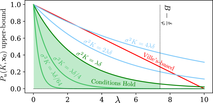
Figure 2: Comparison for Prop. 1 with $B=10,K=100,\delta=1,$ and varying $\sigma$ and $\lambda$. The Freedman-based bounds are shown in green when the conditions of Thm. 1 hold and blue when they do not. The Ville’s-based bound is shown in red. Code to reproduce this plot can be found at [5]

Figure 3: Probability that the system is unsafe: our bound from Cor. 1 (blue), ISSf bound (red). The $x$-axis is the level set expansion $-\epsilon$ and the $y$-axis is the failure probability (lower is better). The plots from left to right indicate safety for $K=1,100,200,300,$ and $400$ steps. Simulations where $\mathbb{E}[h(\mathbf{x}_{k})|\mathscr{F}_{k-1}]=\alpha h(\mathbf{x}_{k})$ and approximate probabilities from 1000 samples are shown for simulations where $h(\mathbf{x}_{k})$ is sampled from 3 different conditional distributions: uniform (pink), truncated Gaussian (green), and a categorical (yellow) all which satisfy Cor. 1. Code for these plots is can be found at [5].

We now seek to relate the Freedman-based bounds proposed in Thm. 3 to the Ville’s-based bounds in Thm. 1. For functions $h$ that have an upper-bound (10), a lower-bounded error (14), and a bounded conditional variance (15), we show there exists a range of values for $\sigma,\delta,K,B,$ and $\lambda$ where the bounds given by Thm. 3 are stronger.

Proposition 1.

For some $\sigma,\delta,B>0$, $\lambda\geq 0$ and $K\in\mathbb{N}_{1}$, consider the conditions

$$\lambda\delta\geq\sigma^{2}K, \lambda\leq B-\frac{\delta}{\varphi},$$ (31)

where $\varphi=2\ln(2)-1$. If these conditions hold, then

$$H\left(\frac{\lambda}{\delta},\frac{\sigma\sqrt{K}}{\delta}\right)\leq 1-\frac{\lambda}{B}.$$ (32)

Proof of this Proposition is is provided in the Appendix.

Intuitively, conditions (31) stipulate that the conditional variance $\sigma^{2}$ and number of steps $K$ must be limited by $\lambda\delta$, which is a function of the initial condition times the maximum single-step disturbance to $h(\mathbf{x}_{k})$. Additionally, the initial condition must be less than the maximum safety bound $B$ by an amount proportional to $\delta$. The exact value of $\varphi$ is a result of the first assumption $(\lambda\delta\geq\sigma^{2}K$) and alternative values can be found by changing this assumption; for clarity of presentation, we leave exploration of these alternative assumptions to future work. The safety bounds for various $\lambda$ and $\sigma$ are shown in Fig. 2 where it is clear that these conditions provide a conservative set of parameters over which this proposition holds.

III-C Extending Input-to-State Safety

Since Thm. 3 assumes that $h$ has lower-bounded differences (14), we can directly compare our probabilistic bounds with the existing Input-to-State Safety (ISSf) [2] method, which provides almost-sure safety guarantees.

In the context of our stochastic, discrete-time problem setting, the ISSf property can be reformulated as:

Proposition 2 (Input-to-State Safety).

If the closed-loop system (2) satisfies the DTCBF condition and the bounded-jump condition (14) (a.s) for some $\alpha\in[0,1)$ and $\delta>0$, then $h(\mathbf{x}_{k})\geq\alpha^{k}h(\mathbf{x}_{0})-\sum_{i=0}^{k-1}\alpha^{i}\delta$ for all $k\geq 0$ and $\mathcal{C}_{\delta}=\left\{\mathbf{x}\in\mathbb{R}^{n}~{}|~{}h(\mathbf{x})\geq\frac{-\delta}{1-\alpha}\right\}$ is safe (a.s.).

Proof.

By combining the bounds (DTCBF) and (14):

$$h(\mathbf{x}_{k+1})\geq\mathbb{E}[h(\mathbf{x}_{k+1})~{}|~{}\mathscr{F}_{k}]-\delta\geq\alpha h(\mathbf{x}_{k})-\delta\textup{ (a.s.)}$$ (33)

Thus, for all $k\in\mathbb{Z}$, we have the lower-bound $h(\mathbf{x}_{k})\geq\alpha^{k}h(\mathbf{x}_{0})-\sum_{i=0}^{k-1}\alpha^{i}\delta$ (a.s). Furthermore, for all time, $h(\mathbf{x}_{k})\geq\frac{-\delta}{1-\alpha}\implies h(\mathbf{x}_{k+1})\geq\frac{-\delta}{1-\alpha}$, so $\mathcal{C}_{\delta}$ is safe (a.s.). ∎

To compare with ISSf’s worst-case expanded safe set $\mathcal{C}_{\delta}$, we wish to use Thm. 3 to bound the probability that our system leaves any expanded safe set $\mathcal{C}_{\epsilon}=\{\mathbf{x}\in\mathbb{R}^{n}|h(\mathbf{x})\geq-\epsilon\}$ with $\epsilon\geq 0$ in finite time.

Corollary 1.

If the hypotheses of Theorem 3 are satisfied and (2) satisfies the DTCBF for some $\alpha\in(0,1)$, then for any value $\epsilon\geq 0$ and any $K\in\mathbb{N}_{1}$,

$$P \bigg{\{}\min_{k\leq K}\;h(\mathbf{x}_{k})<-\epsilon\bigg{\}}$$ (34)

$$\leq H\left(\lambda,\frac{\sigma}{\delta}\left(\frac{1-\alpha^{2K}}{1-\alpha^{2}}\right)^{\frac{1}{2}}\right)\mathds{1}_{\left\{-\epsilon\geq\alpha^{K}h(\mathbf{x}_{0})-\sum_{i=0}^{K-1}\alpha^{i}\delta\right\}}$$

where $\lambda=\frac{\alpha^{K}}{\delta}(h(\mathbf{x}_{0})+\epsilon)$.

Proof.

The DTCBF condition ensures that, for any $\epsilon\geq 0$:

$$\mathbb{E}[~{}h(\mathbf{x}_{k+1})+\epsilon~{}|~{}\mathscr{F}_{k}~{}] \geq\alpha(h(\mathbf{x}_{k})+\epsilon)+\epsilon(1-\alpha)$$ (35)

$$\geq\alpha(h(\mathbf{x}_{k})+\epsilon)$$ (36)

We apply the same proof as Thm. 3 starting at (19) with ($\eta(\mathbf{x}_{k})=\frac{h(\mathbf{x}_{k})+\epsilon}{\delta},\tilde{\alpha}=\alpha,\tilde{c}=0$). Choosing $\lambda=\alpha^{K}\eta(\mathbf{x}_{0})$ and bounding $\langle M\rangle_{K}\leq\sum_{i=1}^{K}\alpha^{2(K-i)}\frac{\sigma^{2}}{\delta^{2}}=\frac{\sigma^{2}(1-\alpha^{2K})}{\delta^{2}(1-\alpha^{2})}$ as in (24) yields the desired bound without the indicator function by applying Thm. 2. The indicator function is a result of applying the lower bound on the safety value from Prop. 1, i.e. $h(\mathbf{x}_{k})\geq\alpha^{k}h(\mathbf{x}_{0})-\sum_{i=0}^{k-1}\alpha^{i}\delta$ (a.s.) for $k\in\mathbb{Z}$. ∎

A comparison of the bounds from Prop. 1 and Cor. 2 and Monte Carlo approximations for various $\epsilon$ and a variety of distributions is shown in Fig. 3.

For these simulations, we use the simple system:

$$\mathbf{x}_{k+1}=\alpha\mathbf{x}_{k}+\mathbf{d}_{k}$$ (37)

for $\mathbf{x}\in\mathbb{R}^{1}$, $\alpha=0.99$, and zero-mean disturbances $\mathbf{d}_{k}$ sampled from a variety of distributions for up to $K=400$ steps. This system naturally satisfies the DTCBF constraint:

$$\mathbb{E}[h(\mathbf{x}_{k+1})|\mathscr{F}_{k}]\geq\alpha h(\mathbf{x}_{k})\textup{ with }h(\mathbf{x})=\mathbf{x},$$ (38)

so we seek to provide guarantees of its inherent safety probabilities. In particular, in three different experiments we consider $\mathbf{d}_{k}$ sampled from one of three zero-mean distributions that all satisfy $|\mathbf{d}|\leq 1$ and $\sigma\leq\frac{1}{3}$: a uniform distribution $\mathcal{U}_{[-1,1]}$, a standard normal distribution truncated at $-1$ and $1$, and a categorical distribution where $\mathbb{P}\{\mathbf{d}=-1\}=\frac{1}{6}$ and $\mathbb{P}\{\mathbf{d}=\frac{1}{5}\}=\frac{5}{6}$ to ensure 0 mean.

These simulations show that although our method is conservative compared to the Monte-Carlo approximations, it provides useful risk-based safety probabilities for a variety of $\mathcal{C}_{\epsilon}$ level sets whereas ISSf only provides a worst-case almost-surely bound.

IV Case Study: Bipedal Obstacle Avoidance

In this section we apply our method to a simplified model of a bipedal walking robot. In particular, the Hybrid Linear Inverted Pendulum (HLIP) model [28] approximates a bipedal robot as an inverted pendulum with a fixed center of mass (COM) height $z_{0}\in\mathbb{R}>0$. Its states are the planar position, relative COM-to-stance foot position, and COM velocity $\mathbf{p},\mathbf{c},\mathbf{v}\in\mathbb{R}^{2}$. The step-to-step dynamics are linear and the input is the relative foot placement, $\mathbf{u}_{k}\in\mathbb{R}^{2}$. The matrices $\mathbf{A}\in\mathbb{R}^{6\times 6}$ and $\mathbf{B}\in\mathbb{R}^{6\times 2}$ are determined by gait parameters including the stance and swing phase periods, and $z_{0}$. The HLIP model with an added disturbance term, $\mathbf{d}$ is:

$$\mathbf{x}_{k+1}=\mathbf{A}\mathbf{x}_{k}+\mathbf{B}\mathbf{u}_{k}+\mathbf{D}\mathbf{d}_{k},\quad\mathbf{d}_{k}\sim\mathcal{D}.$$

where $\mathbf{x}_{k}=\begin{bmatrix}\mathbf{p}_{k}^{\top}&\mathbf{c}_{k}^{\top}&\mathbf{v}_{k+1}^{\top}\end{bmatrix}^{\top}$. We augment the standard HLIP model and assume that $\mathbf{d}$ enters the system linearly and that $\mathcal{D}$ is a $4$-dimensional, $0$-mean uniform distribution where $|\mathbf{d}^{i}|\leq d_{\textup{max}}$ for each $i$ component of $\mathbf{d}$.

We define safety for this system as avoiding a circular obstacle of radius $r>0$ located at $(x,y)=\boldsymbol{\rho}\in\mathbb{R}^{2}$, so safety can be defined using the signed-distance function $h(\mathbf{x})=\|\mathbf{p}-\boldsymbol{\rho}\|_{2}-r$. Notably, this function has no upper bound and therefore the Ville’s-based Thm. 1 does not apply.

Since $h(\mathbf{x})$ is not convex, we use a conservative halfspace convexification instead:

$$h(\mathbf{x}_{k+1})\geq\widehat{\mathbf{e}}(\mathbf{p}_{k})^{\top}\left(\mathbf{p}_{k+1}-\boldsymbol{\rho}\right)-r\triangleq\bar{h}(\mathbf{x}_{k+1}),$$ (39)

where $\widehat{\mathbf{e}}(\mathbf{p})=\frac{(\mathbf{p}-\boldsymbol{\rho})}{\|\mathbf{p}-\boldsymbol{\rho}\|}$ and we apply the controller:

$$\mathbf{u}^{*}=\min_{\mathbf{u}\in\mathbb{R}^{2}} \quad\|\mathbf{u}-\mathbf{k}_{\textup{nom}}(\mathbf{x}_{k})\|$$ (40)

s.t. $$\quad\mathbb{E}\left[~{}\bar{h}(\mathbf{x}_{k+1})~{}|~{}\mathscr{F}_{k}~{}\right]\geq\alpha\bar{h}(\mathbf{x}_{k})$$

with $\alpha\in(0,1]$ and where $\mathbf{k}_{\textup{nom}}$ tracks a desired velocity.

We ran 5000 trials with 3 steps per second and compared against the theoretical bound from Thm. 3. Those values and planar pose trajectories can be seen in Fig. 1. Exact values and code for this and all other plots can be found in at [5].

V Conclusion

Despite the relative tightness guarantee of Proposition 1, the probability guarantees of our method are not necessarily tight as can be seen in Fig. 3. Optimization of $h$ without changing $\mathcal{C}$ as in [11] is a promising direction further tightening of our bound. Additionally, the case study shown in Section IV presents an immediate direction for future work which may involve learning the real-life disturbance distribution as in [18] on a humanoid robot such as [29].

-A Proof of Ville’s Inequality

Proof.

Fix $\lambda>0$ and define the stopping time $\tau\triangleq\inf\{k\in\mathbb{N}~{}|~{}W_{k}>\lambda\}$ with $\tau=+\infty$ if $W_{k}\leq\lambda$ for all time. Since $W_{k}$ is a nonnegative supermartingale, the stopped process $W_{k\wedge\tau}$ is also a nonnegative supermartingale where

$$\mathbb{E}[W_{k\wedge\tau}]\leq\mathbb{E}[W_{0}]\textup{ and }\liminf_{k\to\infty}\mathbb{E}[W_{k\wedge\tau}]\leq\mathbb{E}[W_{0}].$$ (41)

We can further bound this in the case that $\tau$ is finite:

$$\mathbb{E}[W_{0}] \geq\liminf_{k\to\infty}\mathbb{E}[W_{k\wedge\tau}\mathds{1}_{\{\tau<\infty\}}]$$ (42)

$$\geq\mathbb{E}[\liminf_{k\to\infty}W_{k\wedge\tau}\mathds{1}_{\{\tau<\infty\}}]$$ (43)

$$>\mathbb{E}[\lambda\mathds{1}_{\tau<\infty}]=\lambda\mathbb{P}\{\tau<\infty\}=\lambda\mathbb{P}\left\{\sup_{k\in\mathbb{N}}W_{k}>\lambda\right\}.$$

The first inequality is by the nonegativity of $W_{k}$, the second inequality is by Fatou’s Lemma [26], and the third is by the definition of $\tau$. Rearranging terms completes the proof. ∎

-B Proof of Theorem 1

Proof.

We prove the two cases separately:

• We first prove the case when (DTCBF) is satisfied. Let $W_{k}\triangleq B\alpha^{-K}-\alpha^{-k}h(\mathbf{x}_{k})$. This is a nonnegative supermartingale for $k\leq K$:

  $$R_{k}=\alpha^{-K}B -\alpha^{-k}h(\mathbf{x}_{k})\geq\alpha^{-k}(B-h(\mathbf{x}_{k}))\geq 0$$

  $$\mathbb{E}[W_{k+1}|\mathscr{F}_{k}] =\alpha^{-K}B-\alpha^{-(k+1)}\mathbb{E}[h(\mathbf{x}_{k+1})|\mathscr{F}_{k}]$$

  $$\leq\alpha^{-K}B-\alpha^{-k}h(\mathbf{x}_{k})=\mathbb{R}_{k}.$$ (44)

  Apply Ville’s inequality 1 to $W_{k}$ to find:

  $$\mathbb{P}\left\{\max_{k\leq K}W_{k}\leq\lambda\right\}\leq\frac{\mathbb{E}[W_{0}]}{\lambda}.$$ (45)

  Next note that the implications:

  $$\exists k\leq K\textup{ s.t. }h(\mathbf{x}_{k})<0\implies\exists k\leq K\textup{ s.t. }W_{k}>\alpha^{-K}B$$

  ensure that $P_{u}(K,\mathbf{x}_{0})\leq\mathbb{P}\left\{\max_{k\leq K}W_{k}>\alpha^{-K}\right\}$. Choose $\lambda=\alpha^{-K}B$ to achieve:

  $$P_{u}(K,\mathbf{x}_{0})\leq\frac{\alpha^{-K}B-h(\mathbf{x}_{0})}{\alpha^{-K}B}=1-\frac{h(\mathbf{x}_{0})}{B}\alpha^{K}$$ (46)

• Next we prove the case when ($c$-mart.) is satisfied. Let $W^{c}_{k}\triangleq B-h(\mathbf{x_{k}})+(K-k)c$. This is a non-negative supermartingale for $k\leq K$:

  $$W^{c}_{k} =B-h(\mathbf{x}_{k})+(K-k)c\geq 0$$ (47)

  $$\mathbb{E}[W^{c}_{k+1}~{}|~{}\mathscr{F}_{k}] =B-\mathbb{E}[h(\mathbf{x}_{k+1})~{}|~{}\mathscr{F}_{k}]+(K-k-1)c$$

  $$\leq B-h(\mathbf{x}_{k})+c+(K-k-1)c$$ (48)

  $$=B-h(\mathbf{x}_{k})+(K-k)c=W^{c}_{k}$$ (49)

  Apply Ville’s inequality 1 to $W^{c}_{k}$ to find:

  $$\mathbb{P}\left\{\max_{k\leq K}W^{c}_{k}\leq\lambda\right\}\leq\frac{\mathbb{E}[W^{c}_{0}]}{\lambda}$$ (50)

  Next note that the implication:

  $$\exists k\leq K\textup{ s.t. }h(\mathbf{x}_{k})<0\implies\exists k\leq K\textup{ s.t. }W^{c}_{k}>B$$

  ensure that $P_{u}(K,\mathbf{x}_{0})\leq\mathbb{P}\{\max_{k\leq K}W^{c}_{k}\leq\lambda\}$. Choose $\lambda=M$ to achieve:

  $$P_{u}(K,\mathbf{x}_{0})\leq\frac{B-h(\mathbf{x}_{0})+Kc}{B}=1-\frac{h(\mathbf{x}_{0})-Kc}{B}.$$

∎

-C Proof of Proposition 1

Proof.

Define $\Delta\left(\lambda,B,\sigma,K,\delta\right)\triangleq 1-\frac{\lambda}{B}-H\left(\frac{\lambda}{\delta},\frac{\sigma\sqrt{K}}{\delta}\right).$

If $\Delta(\lambda,B,\sigma,K,\delta)\geq 0$, then (32) must hold. We first show $\Delta$ is monotonically decreasing in $\sigma^{2}$. Consider $\frac{\partial\Delta}{\partial(\sigma^{2})}=a(\lambda,\sigma,K,\delta)b(\lambda,\sigma,K,\delta)$ where

$$a(\lambda,\sigma,K,\delta) \triangleq\frac{-e^{\frac{\lambda}{\delta}}}{\delta^{2}\sigma^{2}}\left(\frac{\sigma^{2}K}{\lambda\delta+\sigma^{2}K}\right)^{\frac{(\lambda\delta+\sigma^{2}K)}{\delta^{2}}}<0,$$ (51)

$$b(\lambda,\sigma,K,\delta) \textstyle\triangleq\bigg{(}\sigma^{2}K\ln\left(\frac{\sigma^{2}K}{\lambda\delta+\sigma^{2}K}\right)+\lambda\delta\bigg{)}.$$ (52)

The function $a(\lambda,\sigma,K,\delta)$ is negative since $\delta,\sigma,K>0$. For $b(\cdot)$, the logarithm bound $\ln(r)\geq 1-1/r$ ensures that:

$$\textstyle b(\lambda,\sigma,K,\delta)\geq\sigma^{2}K\left(1-\frac{\lambda\delta+\sigma^{2}K}{\sigma^{2}K}\right)+\lambda\delta=0.$$ (53)

Since $a<0$ and $b\geq 0$, $\Delta(\lambda,B,\sigma,K,\delta)$ is monotonically decreasing with respect to $\sigma^{2}$, so we can use the assumption $\sigma^{2}K\leq\lambda\delta$ to lower bound $\Delta$ as:

$$\Delta(\lambda,B,\sigma,K,\delta)\geq 1-\frac{\lambda}{B}-\left(\frac{1}{2}\right)^{2\frac{\lambda}{\delta}}e^{\frac{\lambda}{\delta}}$$ (54)

$$=1-\frac{\lambda}{B}-e^{(1-2\ln(2))\frac{\lambda}{\delta}}\triangleq 1-\frac{\lambda}{B}-e^{-\varphi\frac{\lambda}{\delta}}\triangleq\Delta_{1}(\lambda,B,\delta)$$

where $\varphi\triangleq 2\ln(2)-1>0$.

Next, we show that $\Delta_{1}(\lambda,B,\delta)\geq 0$ for $\lambda\in\left[0,B-\frac{\delta}{\varphi}\right]$. We prove this by showing that $\Delta_{1}(\lambda,B,\delta)\geq 0$ for $\lambda=\left\{0,B-\frac{\delta}{\varphi}\right\}$ and that $\Delta_{1}$ is concave with respect to $\lambda$.

(1) Nonnegativity at $\lambda=0$:   $\Delta_{1}(0,B,\delta)=0.\quad\quad\quad\quad\quad\quad$

(2) Nonnegativity at $\lambda=B-\frac{\delta}{\varphi}$:

$$\Delta_{1} \left(B-\frac{\delta}{\varphi},B,\delta\right)=\frac{\delta}{\varphi B}-e^{-\left(B-\frac{\delta}{\varphi}\right)\frac{\varphi}{\delta}}=\frac{\delta}{\varphi B}-e^{\left(1-\frac{B\varphi}{\delta}\right)}$$

$$\geq\frac{\delta}{\varphi B}-\frac{\delta}{\varphi B}=0,$$ (55)

where the inequality in line (55) is due to the previously used log inequality: $\ln(r)\geq 1-\frac{1}{r}\iff r\geq e^{\left(1-\frac{1}{r}\right)}$, which holds for $r=\frac{\delta}{B\varphi}>0$ since $B,\delta,\varphi>0$.

(3) Concavity for $\lambda\in\left[0,B-\frac{\delta}{\varphi}\right]$: Since $\frac{\varphi}{\delta}>0$, the second derivative of $\Delta_{1}$ with respect to $\lambda$ is negative:

$$\frac{\partial^{2}\Delta_{1}}{\partial\lambda^{2}}=-\left(\frac{\varphi}{\delta}\right)^{2}e^{-\varphi\frac{\lambda}{\delta}}<0.$$ (56)

Thus, $\Delta_{1}$ is concave with respect to $\lambda.$ Since, $\Delta_{1}(0,B,\delta)\geq 0$, $\Delta_{1}\left(B-\frac{\delta}{\varphi},B,\delta\right)\geq 0$, and $\Delta_{1}(\lambda,B,\delta)$ is concave for all $\delta>0$ and $B\geq\frac{\delta}{\varphi}$, it follows from the definition of concavity that $\Delta_{1}(\lambda,B,\delta)\geq 0$ for all $\lambda\in\left[0,B-\frac{\delta}{\varphi}\right].$

Using this lower bound for $\Delta_{1}(\lambda,B)$, we have $\Delta(\lambda,B,\sigma,K,\delta)\geq\Delta_{1}(\lambda,B)\geq 0$ which implies the desired inequality (32).∎

-D Derivative of $\frac{\partial\Delta}{\partial(\sigma^{2})}$

-C Here we show the derivation of the derivative given in (-C). For reference, the complete function is:

$$\Delta(\lambda,B,\sigma,K,\delta)\triangleq 1-\frac{\lambda}{B}-\left(\frac{\sigma^{2}K}{\lambda\delta+\sigma^{2}K}\right)^{\frac{1}{\delta^{2}}(\sigma^{2}K+\lambda\delta)}e^{\frac{\lambda}{\delta}}$$

with the partial derivative with respect to $\sigma^{2}$:

$$\frac{\partial\Delta}{\partial(\sigma^{2})} =-e^{\frac{\lambda}{\delta^{2}}}\frac{\partial}{\partial(\sigma^{2})}\left[u(\sigma^{2})^{v(\sigma)}\right]$$ (57)

$$=-e^{\frac{\lambda}{\delta^{2}}}\frac{u(\sigma^{2})^{v(\sigma^{2})}}{u(\sigma^{2})^{v(\sigma^{2})}}\frac{\partial}{\partial(\sigma^{2})}\left[u(\sigma^{2})^{v(\sigma^{2})}\right]$$ (58)

$$=-e^{\frac{\lambda}{\delta^{2}}}u(\sigma^{2})^{v(\sigma^{2})}\frac{\partial}{\partial(\sigma^{2})}\left[\ln\left(u(\sigma^{2})^{v(\sigma^{2})}\right)\right]$$ (59)

$$=-e^{\frac{\lambda}{\delta^{2}}}u(\sigma^{2})^{v(\sigma^{2})}\frac{\partial}{\partial(\sigma^{2})}\left[\ln\left(u(\sigma^{2})\right)v(\sigma^{2})\right]$$ (60)

$$=-e^{\frac{\lambda}{\delta^{2}}}u(\sigma^{2})^{v(\sigma^{2})}\left[\frac{v(\sigma^{2})}{u(\sigma^{2})}\frac{\partial u}{\partial(\sigma^{2})}+\ln(u(\sigma^{2}))\frac{\partial v}{\partial(\sigma^{2})}\right]$$

$$=-e^{\frac{\lambda}{\delta^{2}}}u(\sigma^{2})^{v(\sigma^{2})}\left[\frac{\lambda}{\delta\sigma^{2}}+\ln(u(\sigma^{2}))\frac{K}{\delta^{2}}\right]$$

$$=\underbrace{-\frac{e^{\frac{\lambda}{\delta^{2}}}}{\delta^{2}\sigma^{2}}u(\sigma^{2})^{v(\sigma^{2})}}_{\triangleq a(\lambda,\sigma,K,\delta)}\underbrace{\left[\lambda\delta+\sigma^{2}K\ln(u(\sigma^{2}))\right]}_{\triangleq b(\lambda,\sigma,K,\delta)}$$ (61)

where introduce the following functions for clarity:

$$u(\sigma^{2})\triangleq\frac{\sigma^{2}K}{\delta\lambda+\sigma^{2}K}, v(\sigma^{2})\triangleq\frac{1}{\delta^{2}}(\lambda\delta+\sigma^{2}K).$$ (62)

Critically, this proof multiplies by 1 in line (58) (which is well defined since $\sigma,\delta,K>0$), then applies the product rule in reverse (59), and then uses the properties of the logarithm function (60). The derivation is finished by applying the product rule and rearranging terms.

References

• [1] A. D. Ames, X. Xu, J. W. Grizzle, and P. Tabuada, “Control Barrier Function Based Quadratic Programs for Safety Critical Systems,” IEEE Transactions on Automatic Control, vol. 62, pp. 3861–3876, Aug. 2017.
• [2] S. Kolathaya and A. D. Ames, “Input-to-State Safety With Control Barrier Functions,” IEEE Control Systems Letters, vol. 3, Jan. 2019.
• [3] S. Bansal, M. Chen, S. Herbert, and C. J. Tomlin, “Hamilton-jacobi reachability: A brief overview and recent advances,” in 2017 IEEE 56th Annual Conference on Decision and Control (CDC), 2017.
• [4] F. Borrelli, A. Bemporad, and M. Morari, Predictive control for linear and hybrid systems. Cambridge University Press, 2017.
• [5] Code Repository for this work:. https://github.com/rkcosner/freedman.git.
• [6] O. So, A. Clark, and C. Fan, “Almost-sure safety guarantees of stochastic zero-control barrier functions do not hold,” 2023. arXiv:2312.02430.
• [7] M. Black, G. Fainekos, B. Hoxha, D. Prokhorov, and D. Panagou, “Safety under uncertainty: Tight bounds with risk-aware control barrier functions,” in IEEE International Conference on Robotics and Automation (ICRA), 2023.
• [8] H. Kushner, “Stochastic Stability and Control.,” Academic Press, New York, 1967.
• [9] R. Cosner, P. Culbertson, A. Taylor, and A. Ames, “Robust Safety under Stochastic Uncertainty with Discrete-Time Control Barrier Functions,” in Proceedings of Robotics: Science and Systems, 2023.
• [10] C. Santoyo, M. Dutreix, and S. Coogan, “Verification and control for finite-time safety of stochastic systems via barrier functions,” in IEEE Conference on Control Technology and Applications (CCTA), 2019.
• [11] J. Steinhardt and R. Tedrake, “Finite-time regional verification of stochastic non-linear systems,” The International Journal of Robotics Research, vol. 31, pp. 901–923, June 2012.
• [12] F. B. Mathiesen, L. Romao, S. C. Calvert, A. Abate, and L. Laurenti, “Inner approximations of stochastic programs for data-driven stochastic barrier function design,” in 2023 62nd IEEE Conference on Decision and Control (CDC), pp. 3073–3080, 2023.
• [13] V. K. Sharma and S. Sivaranjani, “Safe control design through risk-tunable control barrier functions,” in 2023 62nd IEEE Conference on Decision and Control (CDC), pp. 4393–4398, IEEE, 2023.
• [14] A. Singletary, M. Ahmadi, and A. D. Ames, “Safe control for nonlinear systems with stochastic uncertainty via risk control barrier functions,” IEEE Control Systems Letters, vol. 7, pp. 349–354, 2023.
• [15] M. Ahmadi, A. Singletary, J. W. Burdick, and A. D. Ames, “Safe Policy Synthesis in Multi-Agent POMDPs via Discrete-Time Barrier Functions,” in 2019 IEEE Conference on Decision and Control (CDC).
• [16] C. Santoyo, M. Dutreix, and S. Coogan, “A barrier function approach to finite-time stochastic system verification and control,” Automatica, vol. 125, p. 109439, Mar. 2021.
• [17] M. Vahs, C. Pek, and J. Tumova, “Belief control barrier functions for risk-aware control,” IEEE Robotics and Automation Letters, 2023.
• [18] R. K. Cosner, I. Sadalski, J. K. Woo, P. Culbertson, and A. D. Ames, “Generative modeling of residuals for real-time risk-sensitive safety with discrete-time control barrier functions,” May 2023.
• [19] J. Ville, “Etude critique de la notion de collectif,” 1939.
• [20] X. Fan, I. Grama, and Q. Liu, “Hoeffding’s inequality for supermartingales,” Stochastic Processes and their Applications, 2012.
• [21] O. Khatib, “Real-time obstacle avoidance for manipulators and mobile robots,” The international journal of robotics research, 1986.
• [22] A. Agrawal and K. Sreenath, “Discrete Control Barrier Functions for Safety-Critical Control of Discrete Systems with Application to Bipedal Robot Navigation,” in Robotics: Science and Systems XIII, July 2017.
• [23] J. Zeng, B. Zhang, and K. Sreenath, “Safety-Critical Model Predictive Control with Discrete-Time Control Barrier Function,” in 2021 American Control Conference (ACC), pp. 3882–3889, IEEE, May 2021.
• [24] A. J. Taylor, V. D. Dorobantu, R. K. Cosner, Y. Yue, and A. D. Ames, “Safety of sampled-data systems with control barrier functions via approximate discrete time models,” in 2022 IEEE 61st Conference on Decision and Control (CDC).
• [25] P. Culbertson, R. K. Cosner, M. Tucker, and A. D. Ames, “Input-to-State Stability in Probability,” 2023. IEEE Conference on Decision and Control (CDC).
• [26] G. Grimmett and D. Stirzaker, Probability and Random Processes. Oxford University Press, July 2020.
• [27] D. A. Freedman, “On tail probabilities for martingales,” the Annals of Probability, pp. 100–118, 1975.
• [28] X. Xiong and A. Ames, “3-d underactuated bipedal walking via h-lip based gait synthesis and stepping stabilization,” IEEE Transactions on Robotics, vol. 38, no. 4, pp. 2405–2425, 2022.
• [29] A. B. Ghansah, J. Kim, M. Tucker, and A. D. Ames, “Humanoid robot co-design: Coupling hardware design with gait generation via hybrid zero dynamics,” 2023. IEEE Conference on Decision and Control (CDC).