Safe Merging in Mixed Traffic with Confidence
Abstract
In this letter, we present an approach for learning human driving behavior, without relying on specific model structures or prior distributions, in a mixed-traffic environment where connected and automated vehicles (CAVs) coexist with human-driven vehicles (HDVs). We employ conformal prediction to obtain theoretical safety guarantees and use real-world traffic data to validate our approach. Then, we design a controller that ensures effective merging of CAVs with HDVs with safety guarantees. We provide numerical simulations to illustrate the efficacy of the control approach.
Conformal Prediction, Connected and Automated Vehicles, Cyber-Physical Human Systems, and Human-Driven Vehicle Models.
1 Introduction
Connected and automated vehicles (CAVs) promise to revolutionize transportation. With 100% CAV penetration, we can use control algorithms [1] to improve the efficiency [2], safety [3], flow [4], and equity [5] within any transportation network. However, we expect the percentage of deployed CAVs to rise gradually over time. Therefore, there is an urgent need for control approaches that ensure the effective operation of CAVs among human-driven vehicles (HDVs). This is a challenging problem where the inherent uncertainties associated with human driving clash with the need for safety, efficiency, and comfort of any CAV in mixed traffic. Furthermore, any control algorithm deployed in CAVs must allow real-time implementation in diverse situations. Therefore, in this letter, we focus on the control problem in mixed traffic when a CAV seeks to merge from an off-ramp onto a highway among oncoming HDVs.
In recent years, the problem of merging in mixed traffic has attracted considerable attention. Game-theoretic models have been proposed for the interactions between an HDV and an oncoming CAV [6]. Typically, these models consider that the HDV’s driving decisions can be interpreted using a social value orientation that trades off between selfish and altruistic behavior. Such models can yield control algorithms for CAVs that utilize theoretical results from leader-follower games [7] and potential games [8]. Alternatively, HDV behavior can be framed within the context of car-following models, which postulate that HDVs drive in a manner that follows their preceding vehicle within a driving lane. For example, Gibbs’ car following model has been utilized in conjunction with Q-learning to facilitate lane changing of CAVs among HDVs [9]. Similarly, Newell’s car-following model was utilized with Bayesian optimization to derive a control algorithm that facilitates merging in mixed traffic [10]. A typical control approach within all model-based approaches is to learn unknown parameters within the structure of the HDV model and use them to predict the HDV’s future trajectory. Due to the known model structure, these approaches provide uncertainty quantification for human driving and performance guarantees on the eventual control algorithm of the CAV. However, while these control approaches work well in simulation, their guarantees may not hold in practice if actual human driving behavior differs from the implicitly assumed model.
As an alternative to considering specific models for HDVs, data-driven approaches attempt to derive a control strategy with minimal assumptions on human-driving behavior. Deep neural networks with long-short-term memory (LSTM) cells have been proposed as general approximators to learn HDV behavior in various driving scenarios [11, 12]. By leveraging time-series data, these networks can learn the interdependencies of vehicle motion in high-traffic situations [13]. After training a network of sufficient complexity to predict HDV behavior, it is possible to facilitate effective control of CAVs during highway on-ramp merging with control algorithms such as model-predictive control [14] or reinforcement learning algorithms such as deep policy gradient [15]. Reinforcement learning has also served as a model-free approach to computing optimal merging strategies for CAVs directly from data [16, 17]. While such data-driven approaches can learn the complex interactions among HDVs and CAVs, they suffer from a lack of formal guarantees and a lack of interpretability. Thus, their solutions cannot be implemented with confidence within the physical realm.
In this letter, we overcome these challenges by developing a control framework that uses conformal predictions for HDVs to merge data-driven learning with the formal safety guarantees of model-based approaches. Conformal predictions present a calibration methodology to generate set-valued predictions from any black-box model. These set valued predictions are equipped with formal guarantees on the predictive uncertainty [18]. Conformal prediction has been applied to many prediction problems, including dynamic time-series data [19, 20] and hidden Markov models [21] across an infinite time horizon. It has also been utilized for safe model-predictive control with obstacles in robotics [22]. Our primary contributions are (1) the development of a framework integrating conformal predictions into the CAV merging problem and (2) the design of a safe learning and control approach utilizing this framework. A salient feature of our framework is that it can enhance the reliability and safety of CAVs with general assumptions on HDV behavior and without assuming specific prior distributions (e.g., Gaussian).
The remainder of the letter proceeds as follows. In Section 2, we explain our modeling framework of CAV merging on-ramp in mixed traffic scenario. In Section 3, we present a learning approach to predict human-driving behavior and resulting traffic conditions. We introduce conformal prediction and provide a method to incorporate it into the safe merging problem in Section 4. We provide a control strategy for safe merging and demonstrate the effectiveness of the framework through numerical simulations in Section 5. Finally, we draw concluding remarks in Section 6.
2 Modeling Framework
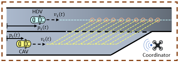
We consider a mixed traffic scenario where a CAV seeks to merge into a highway among oncoming HDVs (see Fig. 1). We define a control zone marked by the dashed boundary in Fig. 1, where we seek to plan the trajectory of the CAV and compute corresponding control inputs. Since CAV-CAV interactions are well understood [3, 4, 2] our focus is on CAV-HDV interactions within the control zone. We consider longitudinal movements only and assume that CAVs can communicate with infrastructure to obtain position and speed information of other vehicles, but the dynamics of HDVs may be unknown to the CAV. Within the control zone, the CAV’s motion is modeled using double integrator dynamics, i.e.,
| (1) | ||||
where is a sampling time, , , and are the position, speed, and control input at time step , respectively. The CAV’s speed and acceleration limits are given by
| (2) | ||||
| (3) |
Let denote the set of HDVs on the highway. For each HDV , the variables and represent position and speed at time , respectively. As time and position have a one-to-one mapping in highway-driving (non-stopping) vehicles, there exists a function that yields a certain time for HDV to arrive at a specific position, i.e., . For a CAV to merge onto the highway, we consider a finite set of merging candidates , where each candidate point is located in index order within a merging lane with equal distances (see Fig. 1). To guarantee safety between HDVs and a CAV at a merging candidate , we impose the time headway constraint
| (4) |
where is the location of merging candidate and is the merging time of the CAV.
For any given merging candidate , we consider that the CAV follows an unconstrained energy-optimal trajectory [3], i.e., its trajectory is described by
| (5) | ||||
where , and are constants of integration, which can be computed using the following boundary conditions
| (6) | ||||
| (7) |
Since from (3), there exists a one-to-one mapping from the position trajectory to the merging time. Consequently, we obtain inverse function with respect to , i.e., . The CAV’s optimization problem is formulated as follows.
Problem 1.
For a CAV to safely merge in between HDVs, we solve the following optimization problem
| (8) | ||||
| subject to: |
The solution to Problem 1 would enable a CAV to safely merge onto highways while minimizing speed transitions, indirectly enhancing energy consumption and comfort. However, solving this problem requires predictions on the time of each HDV to pass each merging candidate . Such predictions are not known a priori and must be obtained from an HDV driving model. Several efforts have been made to learn human-driving models, but these approaches often impose strong assumptions about specific probability distributions or structures for the model [6, 7, 8, 9, 10]. Next, we present a very general model for human driving inspired by Markov decision processes. In subsequent sections, we show how LSTM networks can be employed to learn human-driving behavior and conformal predictions can offer theoretical guarantees to the learned model.
2.1 Human Driving Behavior
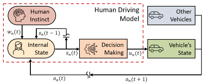
We consider a decision-making process for HDVs as illustrated in Fig. 2. The observation of each HDV at any time is , where denotes the vehicle leading the HDV , is the vehicle preceding the HDV , and is the state of a vehicle at time . The driver of HDV also receives an instinctive driving impulse, modeled as an uncontrolled disturbance that takes values in a set . This disturbance captures the inherent stochasticity of human driving, and we consider that is a sequence of independent variables. Finally, we denote the internal state of the driver of HDV at time by and consider this internal state to be an abstract representation of the current driving intent of the human, including factors such as aggression, biases, conservativeness, attentiveness, etc. To keep our framework general, we do not assume knowledge of the space . However, we do assume that starting with , the internal state evolves as a Markov chain for all :
| (9) |
Based on the internal state, the driver of HDV takes an action . Substituting this action into the vehicle dynamics, the state of HDV evolves as
| (10) |
The primitive variables that determine the motion of HDV through (9) - (10) are . We consider that a CAV receives the observation of the HDV through the coordinator in the control zone. However, the CAV has no knowledge of the internal spaces and , and receives no observations of or for all and all . We impose the following assumptions in our formulation.
Assumption 1.
We consider that the joint prior distribution on the primitive variables of all HDVs is exchangeable when a CAV has no additional information.
Assumption 1 allows us to treat any two primitives from as exchangeable, a property that will be essential to using conformal prediction in Section 4. This assumption implies that re-ordering the HDVs has no effect on the joint distribution, and that a human driver does not distinguish among CAVs and HDVs. Note that, in real world scenarios, a truck may not be exchangeable with a passenger vehicle. However, if features such as vehicle types or driving purpose are available, they can be added to the list of primitives to ensure exchangeability.
Remark 1.
The joint prior on all variables is defined on a probability space , with a sample space , -algebra and probability measure .
Remark 2.
Consider any two random variables and , where is a -algebra on set . Then, and are exchangeable if for any , we have .
Assumption 2.
Human driving behavior is influenced by the behavior of surrounding vehicles, including the leading, rear, and merging vehicles.
In our formulation, we restrict attention to the surrounding vehicles when defining the observation of an HDV and do not consider other environmental or weather-related effects. Considering such factors within the human driving model presents an intriguing direction for future research.
3 Learning Human Driving Behavior
In this section, we present an approach to learn a data-driven model for human driving decisions. To this end, we use an encoder-decoder neural-network architecture with an LSTM, inspired by the notion of approximate information states for partially observed reinforcement learning [23, 14]. The encoder comprises two fully connected linear layers of dimensions and with ReLU activation, followed by an LSTM cell with a hidden state of size denoted by at any . The input to the linear layers at each includes the most recent observation of an HDV , which is supplied as a tuple of the surrounding vehicles’ and its own states. The output of the linear layers is fed into the LSTM in addition to the previous hidden state , and the LSTM’s output is the hidden state at time . Note that as a result of the recursive nature of the LSTM, at each , we can interpret the hidden state of the LSTM as a compression of the history of observations of HDV , i.e., for some compression function , where is the history. Then, we can treat the hidden state of the LSTM as a deterministic approximation of the human’s internal state for all [23, 14]. Subsequently, the output of the encoder is fed into the decoder to generate an estimation of the arrival time of HDV at each merging candidate , i.e., . The decoder consists of sequential modules with two linear layers each with a dimension of and , each layer equipped with ReLU activation.
3.1 Training
We train the network using real-world vehicle trajectories recorded at exits and entries of highways [24]. The dataset was collected with a sampling time of seconds. At each sampling time, we capture the longitudinal positions and speeds of the vehicles on the merging lane and the highway lane adjacent to the merging lane, and we gather that information as a history of observation of each vehicle. Our prediction target comprised the arrival times of these vehicles at all merging candidates (). We utilized the mean-square error as the loss function during training to minimize the discrepancy between our predictions and the target data.
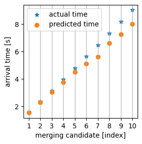
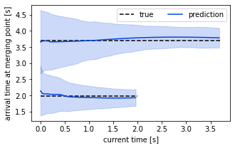
Figure 3 provides an example of the prediction with our trained model, illustrating the predicted (relative) arrival time of an HDV to merging candidates. This visualization highlights the nature of our predictor: within a trajectory, uncertainty diminishes as the predictor accumulates more data.
4 Prediction with Confidence
In this section, we employ conformal prediction on the trained HDV model to obtain a set-valued predictive region for the arrival time of any HDV at a merging candidate . Conformal prediction is a method for establishing such a predictive region for complex or black-box predictive models, such as our encoder-decoder architecture. It provides theoretical guarantees on the uncertainty associated with the predicted range of outputs in the form of a confidence measure without making assumptions on the form of the underlying distribution of the inputs or outputs (e.g., Gaussian). As a consequence, conformal prediction has the potential to enhance the utilization of a trained model in safety-critical applications.
Consider the calibration dataset with data points , where denotes the input and represents the corresponding output. For the next potential data point that we may receive, conformal prediction seeks a set such that with a high probability, i.e.,
| (11) |
where is the confidence in . Furthermore, conformal prediction demands that the set be tighter for predictions likely to be accurate and larger for predictions likely to be inaccurate. Thus, conformal predictions quantify the uncertainty associated with a prediction.
An essential condition for employing conformal prediction to construct a valid set in the above example is that the data should be exchangeable. This assumption is naturally satisfied for static prediction problems such as categorization and labeling. However, its usage on the time series data has been limited due to the inherent non-exchangeability and interdependencies of data points across the trajectory of a time series. Recent research efforts have attempted to overcome this limitation by utilizing adaptive conformal prediction, where the guarantees are asymptotic and may not hold for a finite time horizon [19]. Next, we present an alternate approach to employ conformal prediction specialized to the CAV-HDV merging problem that does not require adaptive prediction and provides tight guarantees.
4.1 Conformal Prediction for Vehicle Merging
In our formulation, since the merging of vehicles occurs within a finite time frame, we can construct a conformal predictor for each . To effectively deploy multiple conformal predictors, we only require two distinct trajectories to be exchangeable and do not need the data to be exchangeable across time within a single trajectory. We will prove in this subsection that exchangeability holds for two distinct trajectories when HDVs follow the general model in Fig. 2.
To begin creating the predictive ranges, we require a calibration dataset distinct from the training data used in Subsection 3.1. We denote this calibration dataset comprising of HDV trajectories as , where represents the history of observations of the -th HDV in the dataset at time , and is the vector of actual arrival times of the -th HDV at all merging candidates during the trajectory. Note that within , the -th HDV is not necessarily the leading vehicle of the -th HDV, as these trajectories are selected randomly from a large collection of trajectories. Next, we prove that under Assumption 1, the arrival times for all HDVs in are exchangeable.
Proposition 1.
Let be the hidden state of an LSTM from Section 3 for any in the dataset , at any . Then, in the corresponding dataset , the tuples and are exchangeable for all , , and .
Proof.
Assumption 1 implies that the primitives of any two HDV’s are exchangeable. Using this assumption with (9) - (10), note that the states and of any two HDVs and are exchangeable for all . Furthermore, since the history of each HDV is a collection of states and the arrival time is a deterministic function of the states and primitives, this also implies that and are exchangeable for all and . Next, consider Borel subsets and for the realizations of the LSTM’s hidden state and HDV’s arrival time at candidate , respectively. Let and . Then, using probability density functions to simplify the notation, , where is the indicator function, , and , and , and is the product of the spaces of the histories. Here, in the first equality, we use the definition of the LSTM’s internal state as a compression of the history, and in the second equality, we use the exchangeability of and . ∎
Proposition 1 enables the use of conformal prediction directly for the input-output pair for any and merging candidate . Given dataset , for each and confidence level , we seek to find a bound for the -the trajectory, such that
| (12) |
where, recall that refers to the decoder of the neural-network trained in Subsection 3.1 and its output is the CAV’s prediction at any time for the arrival time of the -th HDV at candidate . We construct using a standard technique for regression problems [22]. Let be a nonconformity score, which measures the inaccuracy of the prediction. For each HDV and merging candidate , we compute all the nonconformity scores from the given dataset at each . Then, we sort them into ascending order, i.e., we consider the re-ordering of scores such that for all . Then, we determine the conformal bound as
| (13) |
where is the ceiling function.
Remark 3.
Since Proposition 1 establishes the exchangeability of all HDVs, during system operation, the CAV can treat any HDV generating the -th trajectory. Thus, during operation, the conformal range constructed by the CAV at time for the arrival time of HDV at candidate is
| (14) |
For any decoder , this range contains the true arrival time of HDV with probability of [25, Theorem 1].
Using (13), we constructed conformal ranges for the predictions of the neural network trained in Section 3 using calibration trajectories (distinct from the training data) and setting a confidence level of . On validating the performance of the trained model equipped with a conformal predictor over trajectories distinct from both the training and calibration data sets, we observed that across time steps and different merging candidates, the true merging time of an HDV lay within the conformal range of the time. One instance of this testing is illustrated in Fig. 4, where blue solid lines indicate predictions of the HDV’s arrival time at two different merging candidates across , and the shaded area indicates conformal range with confidence level . Note that the conformal range shrinks over time. This is because the prediction uncertainty of the neural network decreases with time as the CAV receives more observations of the HDV’s behavior and better anticipates future actions of the HDV.
Remark 4.
Note that an oncoming CAV merges only at one candidate from . Thus, to guarantee safe merging with the confidence of , it is sufficient to construct a conformal range for each candidate independent of the other candidates. As our approach does not seek guarantees on the prediction of all merging candidates simultaneously, it improves the tightness of our conformal ranges when compared with similar offline approaches that predict complete trajectories, e.g., [22].
5 Safe Merging Strategy
In this section, we introduce a control framework for CAV merging that incorporates the conformal prediction bound . Recall that in constraint (4), Problem 1 requires the actual arrival time from the time trajectory of each HDV for each , which is unknown to the CAV. Thus, at each , the CAV utilizes a model from Subsection 3 to predict the arrival time with a conformal range from Remark 3. Then, the CAV aims to satisfy the following surrogate constraint at each instead of (4):
| (15) |
Note that imposing (15) for all ensures that during the planning at any . Next, we present the CAV’s new merging problem.
Problem 2.
At each , the CAV solves the following optimization problem for a given confidence level
| (16) | ||||
| subject to: |
In Problem 2, the CAV’s goal is to minimize the merging time with confidence level . Note that a feasible solution may not exist in Problem 2 for each . Next, we provide a simple condition to ensure recursive feasibility.
Proposition 2.
Proof.
Generally, the may not hold unless HDVs behave consistently across time. However, if an HDV does behave consistently, this assumption holds for a good predictor that systematically reduces uncertainty with increasing observations, as illustrated in Fig. 4. If no new HDVs enter the control zone beyond those in , recursive feasibility holds under significantly more relaxed conditions because the CAV can slow down to let all HDVs pass before merging.
5.1 Numerical Simulations
To mimic real HDVs in the simulator, we adopt an intelligent driver model (IDM) with some modifications. The acceleration of HDV is given by , where is an acceleration determined from the general IDM, is altruism level of HDV , is the driver’s sensitivity to the CAV, and is the longitudinal distance between HDV and the CAV. An HDV with more altruism tends to yield to the CAV as the longitudinal distance decreases. Less altruistic HDVs ignore the CAV and follow the regular IDM.
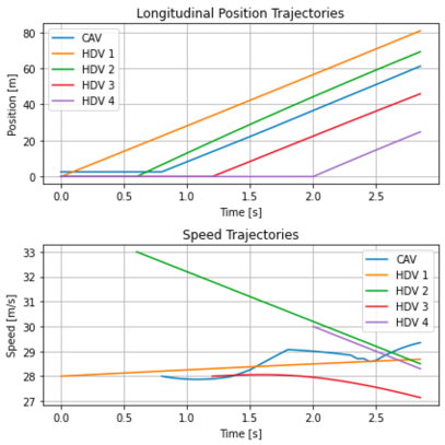
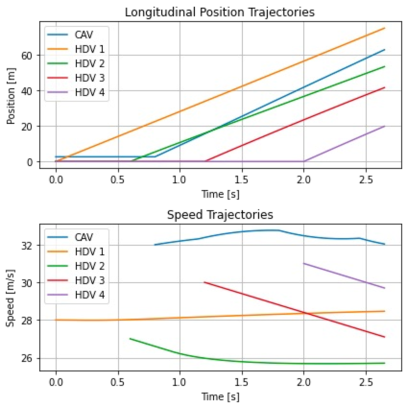
We used the neural network in Section 3 to predict the behavior of each HDV. We trained the network and calibrated the predictions using trajectories for each task. Then, we deployed the network to solve Problem 2 numerically. Figure 5 illustrates two different simulation results, where each column varies in initial speeds and altruism levels for HDVs and maintains the same initial conditions otherwise. In the left column of Fig. 5, the speed profile indicates that the CAV attempted to merge initially between HDVs and but eventually merged behind HDV . In contrast, the right column shows the CAV merging in front of HDV . These distinct behaviors arise from differences in altruism levels among HDVs and . These results demonstrate that our approach allows the CAV to adapt safely to various HDV behaviors.
6 Concluding Remarks
In this letter, we proposed a method of learning human driving behavior without assuming specific structure of prior distributions and employing conformal prediction to obtain theoretical guarantees on the learned model. Utilizing our model, we presented a control framework for a CAV to merge safely in between HDVs. We validated our approach using real-world traffic data and through numerical simulations. An interesting avenue for future work is to dynamically optimize confidence levels and consider more complicated interactions.
References
- [1] A. A. Malikopoulos and L. Zhao, “A closed-form analytical solution for optimal coordination of connected and automated vehicles,” in 2019 American Control Conference (ACC). IEEE, 2019, pp. 3599–3604.
- [2] H. Bang and A. A. Malikopoulos, “A hierarchical approach to optimal flow-based routing and coordination of connected and automated vehicles,” in Proceedings of the 62nd IEEE Conference on Decision and Control (CDC), 2023, pp. 7100–7105.
- [3] A. A. Malikopoulos, L. E. Beaver, and I. V. Chremos, “Optimal time trajectory and coordination for connected and automated vehicles,” Automatica, vol. 125, no. 109469, 2021.
- [4] B. Chalaki, V. Tadiparthi, H. N. Mahjoub, J. D’sa, E. Moradi-Pari, A. S. C. Armijos, A. Li, and C. G. Cassandras, “Minimally disruptive cooperative lane-change maneuvers,” IEEE Control Systems Letters, 2023.
- [5] H. Bang, A. Dave, and A. A. Malikopoulos, “Routing in Mixed Transportation Systems for Mobility Equity,” Proceedings of the 2024 American Control Conference, 2024 (to appear, arXiv:2309.03981).
- [6] W. Schwarting, A. Pierson, J. Alonso-Mora, S. Karaman, and D. Rus, “Social behavior for autonomous vehicles,” Proceedings of the National Academy of Sciences, vol. 116, no. 50, pp. 24 972–24 978, 2019.
- [7] K. Liu, N. Li, H. E. Tseng, I. Kolmanovsky, A. Girard, and D. Filev, “Cooperation-aware decision making for autonomous vehicles in merge scenarios,” in 2021 60th IEEE Conference on Decision and Control (CDC). IEEE, 2021, pp. 5006–5012.
- [8] M. Liu, I. Kolmanovsky, H. E. Tseng, S. Huang, D. Filev, and A. Girard, “Potential game-based decision-making for autonomous driving,” IEEE Transactions on Intelligent Transportation Systems, 2023.
- [9] J. Guo, S. Cheng, and Y. Liu, “Merging and diverging impact on mixed traffic of regular and autonomous vehicles,” IEEE Transactions on Intelligent Transportation Systems, vol. 22, no. 3, pp. 1639–1649, 2020.
- [10] V.-A. Le, B. Chalaki, F. N. Tzortzoglou, and A. A. Malikopoulos, “Stochastic Time-Optimal Trajectory Planning for Connected and Automated Vehicles in Mixed-Traffic Merging Scenarios,” arXiv preprint arXiv:2311.00126, 2023.
- [11] F. Altché and A. de La Fortelle, “An lstm network for highway trajectory prediction,” in 2017 IEEE 20th international conference on intelligent transportation systems (ITSC). IEEE, 2017, pp. 353–359.
- [12] S. H. Park, B. Kim, C. M. Kang, C. C. Chung, and J. W. Choi, “Sequence-to-sequence prediction of vehicle trajectory via lstm encoder-decoder architecture,” in 2018 IEEE intelligent vehicles symposium (IV). IEEE, 2018, pp. 1672–1678.
- [13] N. Deo and M. M. Trivedi, “Convolutional social pooling for vehicle trajectory prediction,” in Proceedings of the IEEE conference on computer vision and pattern recognition workshops, 2018, pp. 1468–1476.
- [14] N. Venkatesh, V.-A. Le, A. Dave, and A. A. Malikopoulos, “Connected and automated vehicles in mixed-traffic: Learning human driver behavior for effective on-ramp merging,” in Proceedings of the 62nd IEEE Conference on Decision and Control (CDC). IEEE, 2023, pp. 92–97.
- [15] Z. el abidine Kherroubi, S. Aknine, and R. Bacha, “Novel decision-making strategy for connected and autonomous vehicles in highway on-ramp merging,” IEEE Transactions on Intelligent Transportation Systems, vol. 23, no. 8, pp. 12 490–12 502, 2021.
- [16] Z. Yan and C. Wu, “Reinforcement learning for mixed autonomy intersections,” in 2021 IEEE International Intelligent Transportation Systems Conference (ITSC). IEEE, 2021, pp. 2089–2094.
- [17] B. Peng, M. F. Keskin, B. Kulcsár, and H. Wymeersch, “Connected autonomous vehicles for improving mixed traffic efficiency in unsignalized intersections with deep reinforcement learning,” Communications in Transportation Research, vol. 1, p. 100017, 2021.
- [18] A. N. Angelopoulos and S. Bates, “Conformal prediction: A gentle introduction,” Foundations and Trends® in Machine Learning, vol. 16, no. 4, pp. 494–591, 2023.
- [19] M. Zaffran, O. Féron, Y. Goude, J. Josse, and A. Dieuleveut, “Adaptive conformal predictions for time series,” in International Conference on Machine Learning. PMLR, 2022, pp. 25 834–25 866.
- [20] K. Stankeviciute, A. M Alaa, and M. van der Schaar, “Conformal time-series forecasting,” Advances in neural information processing systems, vol. 34, pp. 6216–6228, 2021.
- [21] B. Nettasinghe, S. Chatterjee, R. Tipireddy, and M. M. Halappanavar, “Extending conformal prediction to hidden markov models with exact validity via de finetti’s theorem for markov chains,” in International Conference on Machine Learning. PMLR, 2023, pp. 25 890–25 903.
- [22] L. Lindemann, M. Cleaveland, G. Shim, and G. J. Pappas, “Safe planning in dynamic environments using conformal prediction,” IEEE Robotics and Automation Letters, 2023.
- [23] J. Subramanian, A. Sinha, R. Seraj, and A. Mahajan, “Approximate information state for approximate planning and reinforcement learning in partially observed systems,” The Journal of Machine Learning Research, vol. 23, no. 1, pp. 483–565, 2022.
- [24] T. Moers, L. Vater, R. Krajewski, J. Bock, A. Zlocki, and L. Eckstein, “The exid dataset: A real-world trajectory dataset of highly interactive highway scenarios in germany,” in 2022 IEEE Intelligent Vehicles Symposium (IV), 2022, pp. 958–964.
- [25] R. J. Tibshirani, R. Foygel Barber, E. Candes, and A. Ramdas, “Conformal prediction under covariate shift,” Advances in neural information processing systems, vol. 32, 2019.