Abstract

We study Markov potential games under the infinite horizon average reward criterion. Most previous studies have been for discounted rewards. We prove that both algorithms based on independent policy gradient and independent natural policy gradient converge globally to a Nash equilibrium for the average reward criterion. To set the stage for gradient-based methods, we first establish that the average reward is a smooth function of policies and provide sensitivity bounds for the differential value functions, under certain conditions on ergodicity and the second largest eigenvalue of the underlying Markov decision process (MDP). We prove that three algorithms, policy gradient, proximal-Q, and natural policy gradient (NPG), converge to an $\epsilon$-Nash equilibrium with time complexity $O(\frac{1}{\epsilon^{2}})$, given a gradient/differential Q function oracle. When policy gradients have to be estimated, we propose an algorithm with $\tilde{O}(\frac{1}{\min_{s,a}\pi(a|s)\delta})$ sample complexity to achieve $\delta$ approximation error w.r.t the $\ell_{2}$ norm. Equipped with the estimator, we derive the first sample complexity analysis for a policy gradient ascent algorithm, featuring a sample complexity of $\tilde{O}(1/\epsilon^{5})$. Simulation studies are presented.

1 INTRODUCTION

Multi-agent reinforcement learning (MARL) (Busoniu et al.,, 2008; Zhang et al., 2021a, ) features interactions among multiple agents, with each agent having its own objective and decision-making process. It finds applications in various domains, such as video games (Vinyals et al.,, 2019; Samvelyan et al.,, 2019); robotics (Yang and Gu,, 2004; Perrusquía et al.,, 2021); economics (Zheng et al.,, 2022); and networked system control (Chu et al.,, 2020). Unlike single-agent RL, interactions among agents create a dynamic and non-stationary environment, making the learning process more challenging. Under the criterion of discounted reward, theoretical investigations have examined Markov general-sum games (Song et al.,, 2021), zero-sum games (Zhang et al.,, 2020), and Markov potential games (Leonardos et al.,, 2021; Zhang et al., 2021b, ; Ding et al.,, 2022).

In infinite-horizon tasks, it is more natural to use the average reward over the entire life-span for continuing tasks where optimizing stable, long-term performance becomes crucial, e.g., resource allocation in data centers, congestion games, and control problems (Xu et al.,, 2014). As shown in (Zhang and Ross,, 2020), algorithms designed for discounted reward criterion can lead to unsatisfactory performance under the long-term average cost criterion. However, the average reward criterion which suits long-term strategic games remains largely unexplored. This paper delves into the challenges of employing the average reward criterion in the realm of MARL, specifically for Markov potential games.

Among different approaches to reinforcement learning, policy-based methods are appealing due to the ease of applying function approximation for large state and action spaces. However, most of the existing literature on average reward RL is either based on model-based methods (Auer et al.,, 2008; Azar et al.,, 2017), value-based methods (Wei et al.,, 2020), or based on reduction to discounted MDPs (Jin and Sidford,, 2021), with relatively fewer works dedicated to exploring policy-based methods (Li et al.,, 2022; Wei et al.,, 2020). This paper examines policy-based methods in the context of average reward Markov potential games and demonstrates the convergence to a Nash policy, which is the primary goal of theoretical investigations in MARL (Leonardos et al.,, 2021; Ding et al.,, 2022; Zhang et al.,, 2022).

1.1 Contributions

• We address the problem of average reward Markov potential games and analyze three algorithms, policy gradient ascent, proximal-Q, and natural policy gradient. We show that with access to a gradient oracle, they converge to an $\epsilon$-Nash equilibrium with time complexity $O(\frac{1}{\epsilon^{2}})$.

• When the policy gradient has to be estimated, we propose a single-trajectory policy gradient estimator that estimates the policy gradient with $\tilde{O}(\frac{1}{\pi(a|s)\delta})$ sample complexity and $\delta$ approximation error w.r.t. the $\ell_{2}$ norm. We also provide the first sample complexity bound $\tilde{O}(\frac{1}{\epsilon^{5}})$ for the projected policy gradient ascent algorithm.

• On the technical side, we rigorously show that the average reward is an $L$-smooth function of the policy under an ergodicity assumption. This is the first theoretical analysis of policy gradient for the average reward. We note that the concurrent work of Bai et al., (2023) assumes $L$-smoothness without proving it. We also establish sensitivity bounds for differential value functions for general single-agent average reward MDPs, which play an important role in providing regret bound independent of the size of the action set (Section 5). These bounds can potentially be used in smoothness analysis of other parameterized policy parameter classes and function approximation analysis, under a further assumption of (Xu et al.,, 2020, Assumption 1).

Comparison with Previous Works

To obtain a sample complexity bound for a projected policy gradient algorithm, existing work (Leonardos et al.,, 2021) attempts to establish such a bound for a policy projected from a true deterministic gradient, instead of one projected from a gradient estimated from samples (details in Section C.4). The only work that analyzes the estimation error of policy gradient under the average reward setting that we are aware of is a recent work (Bai et al.,, 2023) which separately estimates two parts of policy gradient. Even though they have the same sample complexity, our algorithm calls the estimation algorithm $O(1/\lfloor\frac{1}{\delta}\rfloor)$ times less than theirs, thus reducing the computational burden.

1.2 Related Works

Markov Potential Games

originate from Monderer and Shapley, (1996), who proposed static potential games. Later, Dechert and O’Donnell, (2006) addressed the problem of stochastic lake water usage modeling it as a Markov potential game with known transition probabilities. With the emergence of reinforcement learning, Leonardos et al., (2021) and Zhang et al., 2021b extended the Markov potential game to the unknown dynamics setting, where they analyzed the convergence to Nash equilibrium by extending the policy gradient techniques developed by Agarwal et al., (2021) and Mei et al., (2020) to the multi-agent setting. Later Ding et al., (2022) proposed a policy ascent algorithm, projecting from the Q-function instead of direct policy gradient. Cen et al., (2022), Zhang et al., (2022), and Sun et al., (2024) have studied the natural policy gradient algorithm in the static and Markov settings. Recently, variants of networked Markov potential games and $\alpha$-Markov potential games have been studied by Zhou et al., (2023) and Guo et al., (2023). However, all these results are restricted to the discounted reward setting.

Average Reward MDPs

date back to the classic results of Howard, (1960); Blackwell, (1962); Puterman, (2004); Kakade, (2001); Sutton et al., (1999). When system dynamics are known, average reward MDPs can be solved by linear programming, value iteration, or policy iteration (Howard,, 1960; Puterman,, 2004). A survey can be found in Dewanto et al., (2020). When the dynamics need to be learned, model-based methods like UCRL2 and UCBVI were proposed in Auer et al., (2008) and Azar et al., (2017), and the reward-biased method originally proposed by Kumar and Becker, (1982) has been recently reexamined in Mete et al., (2021). For model-free algorithms, Wei et al., (2020) proposed optimistic mirror ascent, Zhang et al., 2021c studied TD($\lambda$) and Q learning, and Li et al., (2022) analyzed the policy gradient methods under the mirror descent framework. Zhang and Xie, (2023) and Jin and Sidford, (2021) proposed algorithms utilizing a reduction to the discounted reward setting.

2 PRELIMINARIES

In this section, we introduce the average reward Markov potential game (AMPG), Nash equilibria, and differential value functions for the average reward MDP.

2.1 Average Reward Markov Potential Games

An $N$-agent infinite-horizon tabular average-reward Markov game (AMG) is represented by a tuple $\mathrm{AMG}(\mathcal{S},\{\mathcal{A}_{i}\}_{i=1}^{N},P,\{r_{i}\}_{i=1}^{N})$. $\mathcal{S}$ denotes a finite state space, $\mathcal{A}_{i}$ is a finite action space for agent $i$, and $\mathcal{A}=\mathcal{A}_{1}\times\mathcal{A}_{2}\times...\times\mathcal{A}_{N}$ is the joint action space for all agents. We denote by $S$, $A_{1}$, …,$A_{N}$ their respective cardinalities. $P$ denotes the transition probabilities, i.e., $P(\cdot|s,\mathbf{a})\in\triangle(\mathcal{S})$ is the probability distribution of the next state under a joint action profile $\textbf{a}=(a_{1},a_{2},...,a_{N})\in\mathcal{A}$ when the current state is $s$, and $\triangle(\mathcal{S})$ denotes the probability simplex over set $\mathcal{S}$. $r_{i}:\mathcal{S}\times\mathcal{A}\to[0,1]$ is the one-step reward function for agent $i$.

A randomized stationary policy for an agent is defined by a map $\pi_{i}:\mathcal{S}\to\triangle(\mathcal{A}_{i})$, i.e., $\pi_{i}(\cdot|s)\in\triangle(\mathcal{A}_{i})$. Denote by $\Pi_{i}:=(\triangle(\mathcal{A}_{i}))^{\mathcal{S}}$ the set of all randomized policies for agent $i$. We use $\pi=\{\pi_{i}\}_{i=1}^{N}$ to represent the joint policy of all agents, and $\pi_{-i}=\{\pi_{j}\}_{j\neq i}$ to represent all policies but $i$. $\Pi=\Pi_{1}\times\Pi_{2}\times\ldots\times\Pi_{N}$ is the independent joint policy set. Similarly, we denote $a_{-i}:=\{a_{j}\}_{j\neq i}$ and $\Pi_{-i}:=\Pi_{1}\times\ldots\Pi_{i-1}\times\Pi_{i+1}\ldots\times\Pi_{N}$. Under a given joint policy $\pi$, the long-term average reward for agent $i$ starting from initial state $s$ is

$$\rho_{i}^{\pi}(s):=\underset{T\to\infty}{\lim\inf}\frac{1}{T}\mathbb{E}_{\pi}\left[\sum_{t=0}^{T-1}r_{i}(s^{(t)},a^{(t)})|s^{(0)}=s\right].$$ (1)

In this work, we will restrict our attention to an ergodic underlying MDP:

Assumption 1.

For any joint policy $\pi\in\Pi$, the induced Markov chain is irreducible and aperiodic.

Under Assumption 1, there exists a unique stationary distribution $\nu^{\pi}\in\triangle(\mathcal{S})$ independent of the initial state $s$ (Puterman,, 2004) i.e., $\nu^{\pi}(s^{\prime})=\underset{T\to\infty}{\lim}\frac{1}{T}\mathbb{E}_{\pi}\left[\sum_{t=0}^{T-1}\mathbb{I}(s^{(t)}=s^{\prime})|s^{(0)}=s\right]={\lim}_{T\to\infty}\mathbb{E}_{\pi}\left[\mathbb{I}(s^{(T)}=s^{\prime})|s^{(0)}=s\right]$ for any $s\in\mathcal{S}$. As a result, the average reward $\rho_{i}^{\pi}(s)=\langle\nu^{\pi},r_{i}^{\pi}\rangle$ is also independent of the initial state $s$ and we write it as $\rho^{\pi}_{i}$ for simplicity.

Definition 1 (Average reward Markov potential games).

The average reward Markov potential game (ARMPG) is a special case of AMG, where there exists a potential function $\Phi(\pi):\Pi_{1}\times\Pi_{2}\times...\Pi_{N}\to\mathbb{R}$, such that for any $i$, $\pi_{i},\pi_{i}^{\prime}\in\Pi_{i}$ and $\pi_{-i}\in\Pi_{-i}$,

$$\Phi(\pi_{i},\pi_{-i})-\Phi(\pi_{i}^{\prime},\pi_{-i})=\rho_{i}^{\pi_{i},\pi_{-i}}-\rho_{i}^{\pi_{i}^{\prime},\pi_{-i}}.$$

Denote by $C_{\Phi}:=max_{\pi,\pi^{\prime}}|\Phi(\pi)-\Phi(\pi^{\prime})|$ the span of the potential function $\Phi$. Note that $C_{\Phi}\leq N$ since for any joint policies $\pi$ and $\pi^{\prime}$, $|\Phi(\pi)-\Phi(\pi^{\prime})|=|\rho^{\pi}-\rho^{\pi_{1}^{\prime},\pi_{2:N}}+\rho^{\pi_{1}^{\prime},\pi_{2:N}}-\rho^{\pi_{1,2}^{\prime},\pi_{3:N}}+\ldots+\rho^{\pi_{1:N-1}^{\prime},\pi_{N}}-\rho^{\pi^{\prime}}|\leq N$.

Definition 2 (Nash and $\epsilon$-Nash equilibrium).

A policy $\pi^{*}$ is a Nash equilibrium if for each agent $i$,

$$\rho^{\pi^{*}_{i},\pi^{*}_{-i}}\geq\rho^{\pi_{i},\pi^{*}_{-i}},\quad\forall\pi_{i}\in\Pi_{i},$$

or an $\epsilon$-Nash equilibrium if

$$\rho^{\pi^{*}_{i},\pi^{*}_{-i}}\geq\rho^{\pi_{i},\pi^{*}_{-i}}-\epsilon,\quad\forall\pi_{i}\in\Pi_{i}.$$

It may be noted that the maximizer of the potential function is a Nash equilibrium, while the converse may not be true since there could be multiple Nash equilibria.

2.2 Value Functions and Their Properties

The differential value function

$$V^{\pi}_{i}(s):=\mathbb{E}_{\pi}\left[\sum_{t=0}^{\infty}(r_{i}(s^{(t)},\textbf{a}^{(t)})-\rho^{\pi}_{i})|s^{(0)}=s\right]$$ (2)

captures the accumulated deviation from the stationary performance. The differential Q function and differential advantage function are defined respectively as:

$$Q^{\pi}_{i}(s,\textbf{a}):=\mathbb{E}_{\pi}\left[\sum_{t=0}^{\infty}(r_{i}(s^{(t)},\textbf{a}^{(t)})-\rho^{\pi}_{i})|s^{(0)}=s,\textbf{a}^{(0)}=\textbf{a}\right],$$

$$A^{\pi}_{i}(s,\textbf{a}):=Q^{\pi}_{i}(s,\textbf{a})-V^{\pi}(s,\textbf{a}).$$

Taking the expectation with respect to other policies except $j$, we can describe how agent $j$ affects $Q_{i}^{\pi}$ by:

$$\overline{Q}^{\pi}_{j;i}(s,a_{j}):=\underset{a_{-j}\in\mathcal{A}_{-j}}{\sum}\pi_{-j}(a_{-j}|s)Q^{\pi}_{i}(s,a_{j},a_{-j}).$$ (3)

To simplify notation, we will use $\overline{Q}^{\pi}_{i}$ to represent $\overline{Q}^{\pi}_{i;i}$, and define $r_{i}^{\pi}(s):=E_{\mathbf{a}\sim\pi(\cdot|s)}r_{i}(s,\mathbf{a})$, $r_{i}^{\pi_{-j}}(s,a_{j}):=E_{a_{-j}\sim\pi_{-j}(\cdot|s)}r_{i}(s,a_{j},a_{-j})$, and $\overline{A}^{\pi}_{i}(s,a_{i}):=\underset{a_{-i}\in\mathcal{A}_{-i}}{\sum}\pi_{-i}(a_{-i}|s)A^{\pi}_{i}(s,a_{i},a_{-i})$.

With $P_{\pi}\in\mathbb{R}^{S\times S}$ denoting the state transition probability matrix induced by policy $\pi$, and $P^{\pi}\in\mathbb{R}^{SA\times SA}$ denoting the induced state-action transition probability matrix, the differential value function $\mathbf{V_{i}^{\pi}}$ and differential Q function $\mathbf{Q_{i}^{\pi}}$ are solutions of the following equations, up to a constant shift (Puterman,, 2004):

$$\mathbf{V^{\pi}} =\mathbf{r}_{i}^{\pi}-\rho_{i}^{\pi}\mathbf{1}_{S}+P_{\pi}\mathbf{V^{\pi}},$$ (4)

$$\mathbf{Q^{\pi}} =\mathbf{r}_{i}-\rho_{i}^{\pi}\mathbf{1}_{SA}+P^{\pi}\mathbf{Q^{\pi}}.$$

Lemma 1 (Performance difference lemma).

For any policies $\pi_{j}$, $\pi_{j}^{\prime}$ $\in\Pi_{j}$, and $\pi_{-j}\in\Pi_{-j}$, the difference between the average rewards for each agent $i$ is

$$\rho_{i}^{\pi_{j},\pi_{-j}}-\rho_{i}^{\pi^{\prime}_{j},\pi_{-j}}$$

$$= \mathbb{E}_{s\sim\nu^{\pi_{j},\pi_{-j}}}\langle\overline{Q}_{j:i}^{\pi^{\prime}_{j},\pi_{-j}}(s,\cdot),\pi_{j}(\cdot|s)-\pi^{\prime}_{j}(\cdot|s)\rangle$$

$$= \mathbb{E}_{s\sim\nu^{\pi_{j},\pi_{-j}}}\sum_{a_{j}}\pi_{j}(a_{j}|s)\overline{A}_{j:i}^{\pi^{\prime}_{j},\pi_{-j}}(s,a_{j}).$$

Let $\overrightarrow{\mathbf{e}}(s,a_{j})\in\{0,1\}^{S\times A_{j}}$ denote the unit vector where the only non-zero term has the index $(s,a_{j})$. With the definition of Fréchet derivative (Dieudonné,, 2011), we can verify that there exists a linear operator $\mathbf{A}:=\sum_{s}\nu^{\pi}(s)\sum_{a_{j}}\overrightarrow{\mathbf{e}}(s,a_{j})\overline{Q}_{j;i}^{\pi}(s,a_{j})$ mapping the set $U=\{u\in\mathbb{R}^{S\times A_{j}}:\sum_{a\in\mathcal{A}_{j}}u(s,a_{j})=0,\ \forall s\in\mathcal{S}\}$ to $\mathbb{R}^{S\times A_{j}}$ s.t. $\lim_{\lVert u\rVert_{2}\to 0}\frac{\lVert\rho^{\pi_{j}+u,\pi_{-j}}-\rho_{i}^{\pi_{j},\pi_{-j}}-\langle\mathbf{A},u\rangle\rVert_{2}}{\lVert u\rVert_{2}}=0$. This can be shown by the performance difference lemma.

Lemma 2 (Partial derivative).

For any $i,j$, and any policies $\pi_{j}\in\Pi_{j}$, $\pi_{-j}\in\Pi_{-j}$,

$$\frac{\partial\rho_{i}^{\pi}}{\partial\pi_{j}(a_{j}|s)}=\overline{Q}_{j;i}^{\pi}(s,a_{j})\nu^{\pi}(s),$$

$$\frac{\partial\Phi(\pi)}{\partial\pi_{j}(a_{j}|s)}=\overline{Q}_{j}^{\pi}(s,a_{j})\nu^{\pi}(s).$$

Let $\{\lambda_{i}(\mathbf{M})\}_{i=1,...,n}$ be the eigenvalues of matrix $\mathbf{M}\in\mathcal{R}^{n\times n}$, where $|\lambda_{1}(\mathbf{M})|\geq|\lambda_{2}(\mathbf{M})|\geq...\geq|\lambda_{n}(\mathbf{M})|$. The largest eigenvalue of $P^{\pi}$ is 1 corresponding to the eigenvector $\nu^{\pi}P^{\pi}=\nu^{\pi}$ Puterman, (2004). The second largest eigenvalue is strictly less than $1$ and is related to the mixing time of the Markov chain induced by $\pi$ (Kale,, 2013, Lemma 2.1).

Definition 3 (Li et al., (2022)).

Let $1-\Gamma$ be the probability of the least visited state of the MDP, with $\Gamma:=1-\min_{\pi\in\Pi,s\in\mathbb{S}}\nu^{\pi}(s)$. Note that $\Gamma\in(0,1)$.

Definition 4.

The mixing coefficient of the MDP is defined as:

$$\kappa_{0}:=\underset{\pi\in\Pi}{\max}\frac{1}{1-|\lambda_{2}(P^{\pi})|}.$$

Unlike our definitions of $\Gamma$ and $\kappa_{0}$, some literature in the field of average reward MDP employs the concepts of hitting time $t_{hit}:=\max_{\pi}\max_{s}\frac{1}{\nu^{\pi}(s)}$ and mixing time $t_{mix}:=\max_{\pi}\min\{t\geq 1|\lVert(P^{\pi})^{t}(\cdot|s)-\nu^{\pi}\rVert_{1}\leq\frac{1}{4},\forall s\in\mathcal{S}\}$ of the underlying MDP, (Wei et al.,, 2020; Bai et al.,, 2023). We can establish a close relationship between these two sets of definitions. Specifically $\Gamma$ is related to the hitting time as $t_{hit}=\frac{1}{1-\Gamma}$, and from Lemma 3 $\kappa_{0}$ is related to the mixing time as $t_{mix}=O(\frac{1}{\log(1-\frac{1}{\kappa_{0}})})$. It is also evident that $\kappa_{0}$ is finite under Assumption 1 in the tabular setting.

Lemma 3.

Let $C_{p}:=\min\{\sqrt{\frac{S}{1-\Gamma}},\frac{1}{1-\Gamma}\}$ and $\varrho:=1-\frac{1}{\kappa_{0}}$. Then for any policy $\pi$,

$$\sup_{s}\lVert(P^{\pi})^{t}(\cdot|s_{0}=s)-\nu^{\pi}\rVert_{1}\leq C_{p}\varrho^{t},\forall\ t>0.$$

Definition 5.

Define $\kappa:=\max_{i}\max_{\pi}\min_{b\in\mathbb{R}}\lVert\overline{Q}_{i}^{\pi}+b\mathbf{1}\rVert_{\infty}$ for any reward function $r\in[0,1]$.

By Lemma 3, the span of the differential Q function can be bounded as $\kappa\leq\lVert\overline{Q}_{i}^{\pi}\rVert_{\infty}\leq 1+C_{p}\sum_{t=1}^{\infty}\varrho^{t}=1+\frac{C_{p}\varrho}{1-\varrho}\leq C_{p}\kappa_{0}$. Details are in Appendix Proposition 3.

2.3 Performance Metric

We study “independent” policy optimization. By this we mean that at step $t$, each agent $i$ updates its policy $\pi_{i}^{t}$ to $\pi_{i}^{t+1}$ based on the information it can collect locally without coordinating with other agents. The goal is to find a Nash equilibrium, and we quantitatively measure the closeness of the joint policy $\pi^{t}$ to a Nash equilibrium by the $\text{Nash-gap}(t):=\max_{i}\max_{p\in\Pi_{i}}(\rho_{i}^{p,\pi_{-i}^{t}}-\rho_{i}^{\pi_{i}^{t},\pi_{-i}^{t}})$. The optimization algorithm is evaluated by the following notions of Nash regret,

$$\text{Nash-Regret}(T):=\frac{1}{T}\sum_{\tau=0}^{T-1}\text{Nash-gap}(t),$$

$$\text{Nash-Regret}^{*}(T):=\frac{1}{T}\sum_{\tau=0}^{T-1}\text{Nash-gap}(t)^{2}.$$

It is clear that the Nash gap is positive and policy $\pi^{t}$ is an $\epsilon$-Nash equilibrium if $\text{Nash-gap}(t)\leq\epsilon$. Moreover, if the Nash regret (or Nash regret^∗) is less than $\epsilon$, the policy $\pi^{t^{*}}$ with $t^{*}\in\arg\min_{t}\text{Nash-gap}(t)$, is an $\epsilon$ (or $\sqrt{\epsilon}$)-Nash equilibrium.

3 POLICY GRADIENT ALGORITHM

We now analyze the independent projected policy gradient algorithm for average reward Markov potential games. The algorithm adopts a direct policy parameterization. At each step, each agent $i$ updates its policy independently along the gradient direction and projects it back to the policy space via $\text{Proj}_{\Pi_{i}}(\pi):=\arg\min_{p\in\Pi_{i}}\lVert p-\pi\rVert_{2}$.

We first consider the oracle-based setting, where the algorithm has access to a gradient-oracle that can exactly calculate the policy gradient of a given policy. We study the convergence performance in this setting and its time complexity. Subsequently, we consider the setting where there is no access to any oracle. We propose a gradient estimator based on trajectory samples, and study its sample complexity.

The key step in the analysis relies on the smoothness of the average value function. Unlike the discounted setting where the gradient has a closed form expression since $I-\gamma P^{\pi}$ is invertible and its power series can be bounded (Agarwal et al.,, 2021; Leonardos et al.,, 2021), in the average case, a similar analysis can not be applied since $\gamma=1$. In the following Lemma 4, with the help of perturbation theory of stochastic matrices we show that the average reward function is smooth in both single-agent and multi-agent situations. The proof is in Section C.2.

Lemma 4 (Smoothness of $\rho$ and $\Phi$).

Denote $A_{\max}:=\max_{i}A_{i}$, $L:=\kappa_{0}^{2}S^{3/2}A_{\max}+\kappa_{0}\sqrt{S}A_{\max}$, and $L_{\Phi}:=N(\kappa_{0}^{2}S^{3/2}A_{\max}+\kappa_{0}(SA_{\max}+2A_{\max})+A_{\max})$.

(a) For any i, and $\pi_{-i}\in\Pi_{-i}$, the average value $\rho_{i}^{\pi}$ is $\kappa_{0}^{2}S^{3/2}A_{i}+\kappa_{0}\sqrt{S}A_{i}$-smooth with respect to policy $\pi_{i}$. Moreover, for any $i$, $\rho_{i}^{\pi}$ is $L$-smooth with respect to policy $\pi_{i}$, i.e. $\lVert\nabla_{\pi_{i}}\rho_{i}^{\pi_{i},\pi_{-i}}-\nabla_{\pi_{i}}\rho_{i}^{\pi_{i}^{\prime},\pi_{-i}}\rVert_{2}\leq L\lVert\pi_{i}-\pi_{i}^{\prime}\rVert_{2}$ for $\forall\ i,\ and\ \pi_{i},\pi_{i}^{\prime}\in\Pi_{i}$.

(b) The potential function $\Phi(\pi)$ is $L_{\Phi}$-smooth with respect to joint policy $\pi$, i.e. $\lVert\nabla\Phi(\pi)-\nabla\Phi(\pi^{\prime})\rVert_{2}\leq L_{\Phi}\lVert\pi-\pi^{\prime}\rVert_{2}$ for $\forall\ \pi,\pi^{\prime}\in\Pi$.

We note that compared to the smoothness factor in discounted reward settings ($\frac{2\gamma A_{\max}}{(1-\gamma)^{3}}$ for single-agent, $\frac{2N\gamma A_{\max}}{(1-\gamma)^{3}}$ for multi-agent), the smoothness factor for the average reward setting has an extra dependence on state size $S$. The reason is that the second order linear derivative of $\rho^{\pi}$ depends on the $\ell_{1}$ norm of the linear derivative of $\nu^{\pi}$, while Definition 4 can only guarantee an $\ell_{2}$ bound. The exchange between $\ell_{1}$ and $\ell_{2}$ norms introduces the factor $S$.

3.1 Policy Gradient Algorithm with Gradient Oracle

Algorithm 1 Independent projected policy gradient ascent

1:  Input: learning rate $\beta>0$

2:  Initialization: $\pi^{(0)}_{i}(a_{i}|s)=1/A_{i}$ for any $i$, $s$, $a_{i}$

3:  for $t=0$ to $T-1$  do

4:     $\pi_{i}^{(t+1)}=\text{Proj}_{\Pi_{i}}(\pi_{i}^{t}+\beta\nabla_{\pi_{i}}\rho_{i}^{\pi^{t}}),\ \forall i$

5:  end for

We first introduce the distribution mismatch coefficient, which also appears in the convergence behavior of the policy gradient algorithm in discounted single-agent MDPs (Agarwal et al.,, 2021) and discounted Markov potential games (Ding et al.,, 2022; Leonardos et al.,, 2021).

Definition 6 (Distribution mismatch coefficient).

$D:=\max_{\pi,\pi^{\prime}\in\Pi}\lVert\frac{\nu^{\pi}}{\nu^{\pi^{\prime}}}\rVert_{\infty}$.

In the average reward setting, the coefficient $D$ can be upper bounded by $\frac{1}{1-\Gamma}$. The independent projected policy gradient ascent algorithm is given in Algorithm 1, the regret of which is bounded as follows, with its proof given in Section C.2.

Theorem 1.

Choose learning rate $\beta:=\frac{1}{L_{\Phi}}$. Then the Nash-regret* of Algorithm 1 is bounded by

$$\text{Nash-regret}^{*}(T)=O\left(\frac{D^{2}L_{\Phi}C_{\Phi}S}{T}\right).$$

Therefore, by setting time $T:=O\left(\frac{NC_{\Phi}D^{2}S^{5/2}A_{\max}\kappa_{0}^{2}}{\epsilon^{2}}\right)$, it yields an $\epsilon$-Nash equilibrium.

The analysis has two parts. Based on the smoothness estimated in Lemma 4, the algorithm will converge to a stationary point by the optimization theory of gradient ascent. We then show that the stationary policy is a Nash equilibrium in the average reward Markov potential game, which establishes the convergence of the algorithm.

3.2 Sample-Based Policy Gradient Estimate

In practice, we usually do not have access to a gradient oracle. To apply the policy gradient algorithm, we need to estimate the gradient from trajectory samples. We propose a gradient estimator (Algorithm 3) which only relies on a single trajectory and is thus more practical in real applications since it does not require resetting the Markov process or a generative model. The sample-based policy gradient ascent algorithm is described in Algorithm 2.

The estimator $\hat{g}_{i}$ in Algorithm 3 is based on Lemma 2, which relates the policy gradient with $\overline{Q}^{\pi}_{i}(s,a_{i})$, and we approximate it by $R_{i}(t)=\sum_{k=0}^{N}(r_{i}(s^{t+k},\mathbf{a}^{t+k})-\hat{\rho_{i}})$. It is generally hard to estimate the policy gradient in the average reward case. Unlike the discounted reward criterion, the policy gradient might be unbounded under average reward setting. We resolve this issue by adapting the sample length $N$ based on the mixing rate in Lemma 3. However, $\hat{g}_{i}$ may have large variance when $\pi_{i}(a_{i}^{\prime}|s^{\prime})$ is small. To overcome this, we restrict the policy class to $\Pi_{\alpha}:=\Pi_{1,\alpha}\times\ldots\times\Pi_{N,\alpha}$, where $\Pi_{i,\alpha}:=\{(1-\alpha)\pi_{i}+\alpha u_{i}|\forall\pi_{i}\in\Pi_{i}\}$ with $u_{i}:=(\text{Unif}_{\mathcal{A}_{i}})^{S}\in\Pi_{i}$ being the uniform policy. Such restriction has been considered in Leonardos et al., (2021); Ding et al., (2022) previously. We can balance the representation power of the policy class and the variance of the gradient estimator by adjusting $\alpha$.

Algorithm 2 Policy gradient ascent with estimation

1:  Input: learning rate $\beta>0$, $K$, $N_{1}$, $N_{2}$, $N_{3}$

2:  Initialization: $\pi^{(0)}_{i}(a_{i}|s)=1/A_{i}$ for any $i$, $s$, $a_{i}$

3:  for $t=0$ to $T-1$  do

4:     agents take action independently and synchronously for $N_{1}+KN_{2}$ time steps to collect trajectories $\{\mathcal{T}_{i}^{t}\}$

5:     for agent $i$ do

6:        $\hat{g}_{i}^{t}\leftarrow\text{gradient estimation}(\mathcal{T}_{i}^{t},\pi_{i}^{t},K,N_{1},N_{2},N_{3})$

7:        $\pi_{i}^{(t+1)}=\text{Proj}_{\Pi_{i,\alpha}}(\pi_{i}^{t}+\beta\hat{g}_{i}^{t})$

8:     end for

9:  end for

Algorithm 3 Gradient estimation

1:  Input: trajectory $\mathcal{T}=(s^{0},a_{i}^{0},r_{i}^{0},...,s^{t},a_{i}^{t},r_{i}^{t})$, policy $\pi_{i}$, $K$, $N_{1}$, $N_{2}$. ($t=N_{1}+KN_{2}-1$)

2:  $\hat{\rho}_{i}\leftarrow\frac{2}{N_{1}}\sum_{t=\frac{N_{1}}{2}}^{N_{1}-1}r_{i}^{t}$

3:  $g\leftarrow 0$

4:  for $k=0$ to $K-1$ do

5:     $t_{k}\leftarrow N_{1}+kN_{2}$

6:     $R(k)\leftarrow\sum_{\tau=t_{k}}^{t_{k}+N_{2}-1}(r_{i}^{\tau}-\hat{\rho}_{i})$

7:     $g\leftarrow g+R(k)\nabla_{\pi_{i}}\log\pi_{i}(a_{i}^{t_{k}}|s^{t_{k}})$

8:  end for

9:  $\hat{g}_{i}\leftarrow\frac{g}{K}$

10:  Output:$\hat{g}_{i}$

Lemma 5.

For any agent $i$, consider the gradient estimate $\hat{g}_{i}$ defined in Algorithm 3. Given the $(s,a,r)$-trajectory of length $KN_{2}+N_{1}$ and the policy $\pi_{i}\in\Pi_{i,\alpha}$ that generated it, the estimated gradient has $\ell_{2}$ error bounded as

$$\mathbb{E}\lVert\hat{g}_{i}-\frac{\partial\rho_{i}^{\pi}}{\partial\pi_{i}}\rVert_{2}^{2}\leq \left(\frac{1}{\alpha}+1\right)\frac{2A_{\max}N_{2}^{2}}{K}$$

$$+\frac{4C_{p}A_{\max}}{1-\varrho^{N_{2}}}\left(\sqrt{\frac{2}{\alpha}}+\sqrt{2}\right)\frac{N_{2}^{2}}{K}\varrho^{N_{2}}$$

$$+\frac{16A_{\max}C_{p}^{2}}{(1-\varrho)^{2}}\frac{N_{2}^{2}}{N_{1}^{2}}\varrho^{N_{1}}+\frac{2A_{\max}C_{p}^{2}}{(1-\varrho)^{2}}\varrho^{2N_{2}}.$$

We can guarantee an $\ell_{2}$ error of $O(\delta)$ by choosing $N_{1}=N_{2}=O(\log\frac{1}{\delta})$, and $K=\tilde{O}(\frac{A_{\max}}{\alpha\delta})$. A detailed proof is in Section C.3.

Theorem 2.

If all players independently and synchronously run Algorithm 2 with learning rate $\beta=\frac{1}{L_{\Phi}}$, the Nash regret is bounded as:

$$\mathbb{E}[\textnormal{Nash-regret}^{*}(T)]= O{\Big{(}}\frac{D^{2}SL_{\Phi}C_{\Phi}}{T}+\kappa^{2}\alpha^{2}$$

$$+\kappa^{2}DA_{\max}L_{\Phi}^{2}\delta{\Big{)}}.$$

We can therefore determinate an $\epsilon$-Nash equilibrium by choosing $T=O(\frac{NC_{\Phi}D^{2}S^{5/2}A_{max}\kappa_{0}^{2}}{\epsilon^{2}})$, $\alpha=O(\frac{\epsilon}{\kappa})$, $\delta=O(\frac{\epsilon^{2}}{\kappa^{2}DA_{\max}L_{\Phi}^{2}})$, $K=\tilde{O}(\frac{A_{\max}}{\alpha\delta})$, and $N_{1}=N_{2}=\tilde{O}(1)$. Substituting the bound for $\kappa$ and $L_{\Phi}$, the sample complexity is then $T(KN_{2}+N_{1})=\tilde{O}(\frac{N^{3}D^{3}C_{\Phi}S^{7}A_{\max}^{5}\kappa_{0}^{9}}{\epsilon^{5}(1-\Gamma)^{3/2}})$.

To analyze Algorithm 2, we introduce the shadow policy $\tilde{\pi}^{t+1}:=\text{Proj}_{\Pi_{\alpha}}(\pi^{t}+\beta\nabla_{\pi}\Phi(\pi^{t}))$ projected from the true deterministic policy gradient. The distance between $\tilde{\pi}^{t}$ and $\pi^{t}$ is bounded by the estimation error. Since the shadow policy $\tilde{\pi}^{t}$ can capture the optimality criterion in the update rule in Algorithm 2, a bound on the Nash gap with policy improvement w.r.t. potential value can be provided for each time step. Together with the bounded distance from true policy $\pi^{t}$, the conclusion follows.

Remark. We note that there are some mistakes in the analysis of the sample-based policy gradient in (Leonardos et al.,, 2021, Theorem 4.7) about the minimizer of the Moreau envelope and the update analysis, which are elaborated in Section C.4. We address the difficulties in analyzing the sample-based policy gradient algorithm, and as far as we are aware, Theorem 2 is the first sample-based projected policy gradient algorithm for Markov potential games with a rigorous performance guarantee.

4 PROXIMAL-Q ALGORITHM

Algorithm 4 Independent proximal-Q

1:  Input: learning rate $\beta>0$

2:  Initialization: $\pi^{(0)}_{i}(a_{i}|s)=1/A_{i}$ for any $i$, $s$, $a_{i}$

3:  for $t=0$ to $T-1$ do

4:     $\pi_{i}^{t+1}(\cdot|s)=\underset{p(\cdot|s)\in\triangle(\mathcal{A}_{i})}{\arg\max}\{\beta\langle\overline{Q}^{\pi^{t}}_{i}(s,\cdot),p(\cdot|s)\rangle_{\mathcal{A}_{i}}-\frac{1}{2}\lVert p(\cdot|s)-\pi_{i}^{t}(\cdot|s)\rVert_{2}^{2}\}\ \forall s,i$

5:  end for

In this section, we analyze another algorithm, the proximal-Q algorithm, under the assumption of the availability of an oracle for the differential value function. The more general case where there is no oracle, and its sample complexity analysis are addressed in Section D.1. Instead of the policy gradient $\frac{\partial\rho_{i}^{\pi}}{\partial\pi_{i}(a_{i}|s)}=\overline{Q}_{i}^{\pi}(s,a_{i})\nu^{\pi}(s)$, Algorithm 4 uses the differential Q function as the ascent direction, which is less sensitive for states $s$ with a small visiting rate $\nu^{\pi}(s)$. The key part of the regret analysis is to connect the one-step policy update rule with the difference between the respective potential values. The analysis in the discounted setting is based on the performance difference lemma and second order performance difference lemma (Ding et al.,, 2022, Lemma 21), both relying on the backward induction enabled by the discount factor $\gamma<1$, which are unfortunately not applicable in the average reward setting. To bound the second order difference for the average reward, we can use its smoothness property established in Lemma 4, or carefully analyze the sensitivity of the two parts $Q^{\pi}$ and $\nu^{\pi}$ in the performance difference Lemma 1. We emphasize that the sensitivity bounds for differential value functions also play an important role in establishing the regret bound independent of the size of the action set, as shown in Section 5.

Define $\lVert\pi\rVert_{1,\infty}:=\max_{s}\lVert\pi(\cdot|s)\rVert_{1}$ and $\lVert\mathbf{M}\rVert_{\infty}:=\max_{\lVert\mathbf{x}\rVert_{\infty}=1}\lVert\mathbf{Mx}\rVert_{\infty}$ for matrix $\mathbf{M}$. One may note that $\lVert\mathbf{M}_{1}+\mathbf{M}_{2}\rVert_{\infty}\leq\lVert\mathbf{M}_{1}\rVert_{\infty}+\lVert\mathbf{M}_{2}\rVert_{\infty}$, $\lVert\mathbf{M}_{1}\mathbf{M}_{2}\rVert_{\infty}\leq\lVert\mathbf{M}_{1}\rVert_{\infty}\lVert\mathbf{M}_{2}\rVert_{\infty}$, and $\lVert\mathbf{M}\rVert_{\infty}\leq\max_{i}\sum_{j}|\mathbf{M}_{ij}|$.

Let $P^{\pi,\infty}:=((\nu^{\pi})^{T},...,(\nu^{\pi})^{T})^{T}$, with $\nu^{\pi}\in(0,1)^{1\times S}$, denote the infinite-step state transition matrix. There exists a closed form expression $V^{\pi}=(I-P^{\pi}+P^{\pi,\infty})^{-1}(I-P^{\pi,\infty})r^{\pi}$ (Puterman,, 2004).

Definition 7.

For any policy $\pi\in\Pi$, $(I-P^{\pi}+P^{\pi,\infty})$ is invertible (Puterman, (2004)). Define $\kappa_{1}:=\max_{\pi}\lVert(I-P^{\pi}+P^{\pi,\infty})^{-1}\rVert_{\infty}$.

Note that $(I-P^{\pi}+P^{\pi,\infty})^{-1}=I+\sum_{t=1}^{\infty}(P^{\pi}-P^{\pi,\infty})^{t}$. By Lemma 3 and $P^{\pi}P^{\pi,\infty}=P^{\pi,\infty}P^{\pi}=P^{\pi,\infty}$, $P^{\pi,\infty}P^{\pi,\infty}=P^{\pi,\infty}$, we have $\kappa_{1}\leq\lVert I\rVert_{\infty}+\sum_{t=1}^{\infty}\lVert(P^{\pi})^{t}-P^{\pi,\infty}\rVert_{\infty}\leq 1+\sum_{t=1}^{\infty}C_{p}\varrho^{t}=1+C_{p}\frac{\varrho}{1-\varrho}$.

Consider a general average reward MDP with reward function $r$. $\rho_{r}^{\pi}$, $V_{r}^{\pi}$ and $Q_{r}^{\pi}$ can be defined similarly as in Section 2.

Lemma 6 (Sensitivity bounds for average reward MDP).

For any reward function taking values in $[0,1]$, and any policies $\pi,\pi^{\prime}\in\Pi$, the following bounds hold:

$$|\nu^{\pi}(s)-\nu^{\pi^{\prime}}(s)|\leq \kappa\lVert\pi-\pi^{\prime}\rVert_{1,\infty},\ \forall s\in\mathcal{S}$$

$$|\rho^{\pi}_{r}-\rho^{\pi^{\prime}}_{r}|\leq \kappa\lVert\pi-\pi^{\prime}\rVert_{1,\infty},$$

$$\lVert V_{r}^{\pi}-V_{r}^{\pi^{\prime}}\rVert_{\infty}\leq \kappa_{1}(2+S(\kappa+\kappa_{1})+S\kappa\kappa_{1})\lVert\pi-\pi^{\prime}\rVert_{1,\infty},$$

$$\lVert Q^{\pi}_{r}-Q_{r}^{\pi^{\prime}}\rVert_{\infty}\leq (\kappa+2\kappa_{1}+S\kappa_{1}(\kappa+\kappa_{1})+S\kappa\kappa_{1}^{2})$$

$$\times\lVert\pi-\pi^{\prime}\rVert_{1,\infty}.$$

Proofs are provided in Appendix D. Lemma 6 is a general result for both single-agent and multi-agent settings. Consider a joint policy $\pi(\mathbf{a}|s):=\pi_{1}(a_{1}|s)\pi_{2}(a_{2}|s)...\pi_{N}(a_{N}|s)$. If $\pi=(\pi_{j},\pi_{-j})$, $\pi^{\prime}=(\pi^{\prime}_{j},\pi_{-j})$, then $||\pi-\pi^{\prime}||_{1,\infty}=||\pi_{j}-\pi^{\prime}_{j}||_{1,\infty}$. The following proposition is directly derived from Lemma 6.

Proposition 1.

$\lVert Q_{i}^{\pi_{j},\pi_{-j}}-Q_{i}^{\pi_{j}^{\prime},\pi_{-j}}\rVert_{\infty}\leq\kappa_{Q}\lVert\pi_{j}-\pi_{j}^{\prime}\rVert_{1,\infty}$, where $\kappa_{Q}:=\kappa+2\kappa_{1}+S\kappa_{1}(\kappa+\kappa_{1})+S\kappa\kappa_{1}^{2}$.

Theorem 3.

If the learning rate is chosen as $\beta\leq\max\{\frac{1-\Gamma}{(N-1)(\kappa_{Q}+S\kappa^{2})A_{\max}},\frac{1-\Gamma}{2L_{\Phi}}\}$, then Algorithm 4 has a bounded Nash regret:

$$\text{Nash-regret}(T)\leq\sqrt{D}(\kappa\sqrt{A_{max}}+\frac{2}{\beta})\sqrt{2\beta C_{\Phi}}\frac{1}{\sqrt{T}}.$$

If we set the learning rate to $\beta=\frac{1-\Gamma}{2L_{\Phi}}$, the time complexity for an $\epsilon$-Nash equilibrium is $T=O(\frac{NC_{\Phi}DS^{3/2}A_{max}\kappa_{0}^{2}}{(1-\Gamma)\epsilon^{2}})$. The proof is given in Appendix D.

5 NATURAL POLICY GRADIENT

Algorithm 5 Independent natural policy gradient ascent

1:  Input: learning rate $\beta>0$

2:  Initialization: $\pi^{(0)}_{i}(a_{i}|s)=1/A_{i}$ for any $i$, $s$, $a_{i}$

3:  for $t=0$ to $T-1$ do

4:     $\pi_{i}^{t+1}(\cdot|s)=\underset{p(\cdot|s)\in\triangle(\mathcal{A}_{i})}{\arg\max}\{\beta\langle\overline{Q}^{\pi^{t}}_{i}(s,\cdot),p(\cdot|s)\rangle_{\mathcal{A}_{i}}-D^{p}_{\pi_{i}^{t}}(s)\}\ \forall s,i$

5:  end for

Finally, we analyze the natural policy gradient (NPG) algorithm under the average reward setting. NPG is a powerful technique to accelerate the convergence of policy update with Fisher information via preconditioning (Kakade,, 2001). We consider the independent NPG Algorithm 5 under the availability of a differential value function oracle.

Under the softmax parameterization, the joint policy $\pi^{\theta}=(\pi_{1}^{\theta_{1}},\ldots,\pi_{N}^{\theta_{N}})$ with $\theta=(\theta_{1},\ldots,\theta_{N})\in\mathbb{R}^{SA}$ is $\pi^{\theta_{i}}_{i}(s,a)=\frac{\exp(\theta_{s,a_{i}})}{\sum_{a_{i}^{\prime}\in\mathcal{A}_{i}}\theta_{s,a_{i}^{\prime}}}$. The gradient of $\rho$ (or $\Phi$) w.r.t. $\theta$ is $\frac{\partial\rho_{i}^{\pi}}{\partial\theta}=\sum_{s,a}\nu^{\pi}(s)\pi(a|s)\frac{\partial\log\pi(s,a)}{\partial\theta}Q_{i}^{\pi}(s,a)$ (Sutton et al.,, 1999). With the Fisher information matrix defined as $F_{i}(\theta):=\mathbb{E}_{s\sim\nu^{\pi^{\theta}},a_{i}\sim\pi^{\theta_{i}}(\cdot|s)}[(\frac{\partial\log\pi^{\theta_{i}}(a_{i}|s)}{\partial\theta_{i}})(\frac{\partial\log\pi^{\theta_{i}}(a_{i}|s)}{\partial\theta_{i}})^{T}]$ (Kakade,, 2001), the natural policy gradient update is $\theta_{i}^{t+1}=\theta_{i}^{t}+F_{i}(\theta_{i})^{\dagger}\nabla_{\theta_{i}}\rho_{i}^{\pi^{\theta}}.$ It can be shown that the NPG update is equivalent to the update in Algorithm 5 (the proof is provided in Appendix E). In Algorithm 5, $D^{p}_{q}(s):=\sum_{a}p(a|s)\log\frac{p(a|s)}{q(a|s)}$ is the Kullback–Leibler (KL) Divergence between distributions $p(\cdot|s)$ and $q(\cdot|s)$. There is a closed-form expression for the update, $\pi_{i}^{t+1}(a_{i}|s)\varpropto\pi_{i}^{t}(a_{i}|s)\exp\left(\beta\overline{Q}_{i}^{\pi^{t}}(s,a_{i})\right)\varpropto\pi_{i}^{t}(a_{i}|s)\exp\left(\beta\overline{A}_{i}^{\pi^{t}}(s,a_{i})\right)$, which can be verified by the Karush–Kuhn–Tucker (KKT) condition. This does not require the calculation of the inverse of the Fisher information matrix and the gradient oracle, but employs a differential value function oracle instead.

We first show the monotonic improvement property of the NPG one-step update.

Lemma 7.

Let $Z_{t}^{i,s}:=\sum_{a_{i}}\pi_{i}^{t}(a_{i}|s)\exp\left(\beta\overline{A}_{i}^{t}(s,a_{i})\right)$. When $\beta\leq\max\{\frac{1-\Gamma}{(N-1)(\kappa_{Q}+S\kappa^{2})},\frac{1-\Gamma}{L_{\Phi}}\}$,

$$\Phi(\pi^{t+1})-\Phi(\pi^{t})\geq\frac{1}{\beta}\sum_{i}\mathbb{E}_{s\sim\nu^{\pi_{i}^{t+1},\pi_{i}^{t}}}\log Z_{i}^{t,s}\geq 0.$$

In the discounted reward setting, the performance difference lemma provides a bound for the monotone improvement (Zhang et al.,, 2022, Lemma 20) which is applicable only when the potential function $\Phi(\pi)$ can be decomposed as the discounted summation of some state action reward function $\Phi(\pi)=\mathbb{E}_{a\sim\pi,s\sim\eta}\sum_{t}\gamma^{t}\phi(s,a)$. Here we do not need such an additional assumption, but utilize the smoothness (Lemma 4) or the sensitivity bound for differential Q function (Lemma 6) instead.

Let $c(t):=\min_{i}\min_{s}\sum_{a_{i}^{*}\in argmax_{a_{i}\in\mathcal{A}_{i}}\overline{Q}_{i}^{\pi^{t}}(s,a_{i})}\pi^{t}_{i}(a_{i}|s)$, which is also considered in Zhang et al., (2022). It indicates the exploration power of the policy $\pi_{t}$, i.e., the probability mass covering the optimal actions. Define $c:=\inf_{t}c(t)$. The following lemma shows that $c$ is strictly positive, which is key to bounding the convergence rate. The proofs are given in Appendix E.

Lemma 8.

If all stationary points of the potential function $\Phi(\theta)=\Phi(\pi(\theta))$ are isolated, $\beta\leq\min\{\max\{\frac{1-\Gamma}{(N-1)(\kappa_{Q}+S\kappa^{2})},\frac{1-\Gamma}{L_{\Phi}}\},\frac{1}{2\kappa}\}$, Algorithm 5 asymptotically converges to a Nash equilibrium. Then $c>0$.

Theorem 4.

If all stationary points of the potential function $\Phi(\theta)=\Phi(\pi(\theta))$ are isolated, $\beta\leq\min\{\max\{\frac{1-\Gamma}{(N-1)(\kappa_{Q}+S\kappa^{2})},\frac{1-\Gamma}{L_{\Phi}}\},\frac{1}{2\kappa}\}$, the regret of Algorithm 5 can be bounded as

$$\text{Nash-regret}^{*}(T)\leq\frac{3C_{\Phi}}{c\beta(1-\Gamma)T}.$$

Substituting the bound for $\kappa$ and $\kappa_{Q}$, $\beta=\frac{1-\Gamma}{NS^{3/2}\kappa_{0}^{2}\min\{A_{\max},\frac{S^{2}\kappa_{0}}{(1-\Gamma)^{7/2}}\}}$, the time complexity is $T=O(\frac{NC_{\Phi}S^{3/2}\kappa_{0}^{2}\min\{\frac{S^{2}\kappa_{0}}{(1-\Gamma)^{7/2}},A_{\max}\}}{c(1-\Gamma)^{2}\epsilon^{2}})$. When the action set has a large cardinality $A_{\max}$, it gives an $A_{\max}$-independent bound for the chosen learning rate.

6 EXPERIMENTS

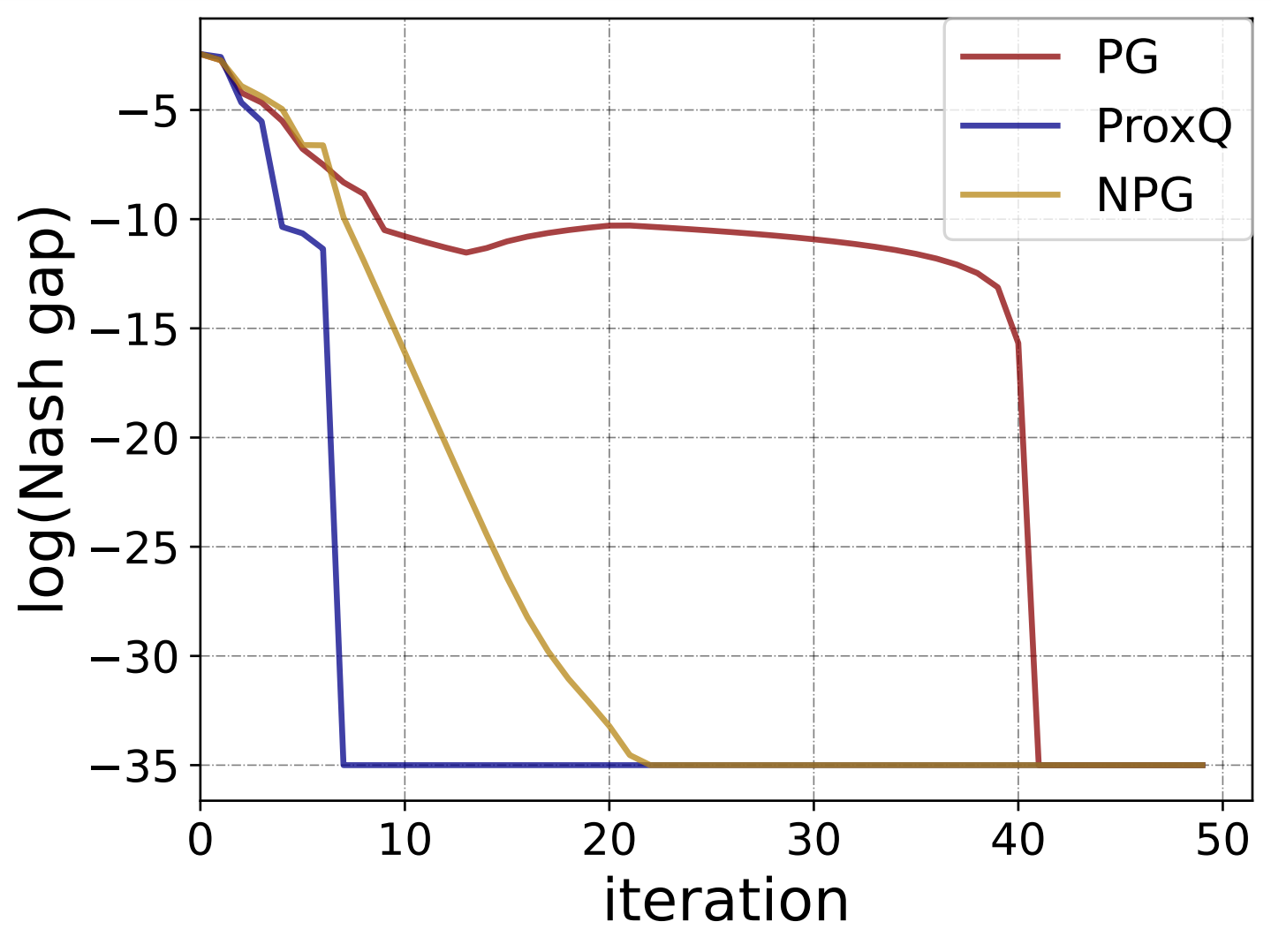
(a) Large LVR, large RG

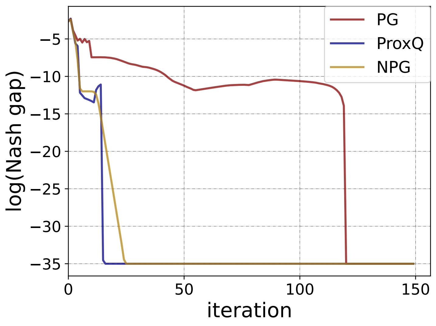
(b) Small LVR, large RG

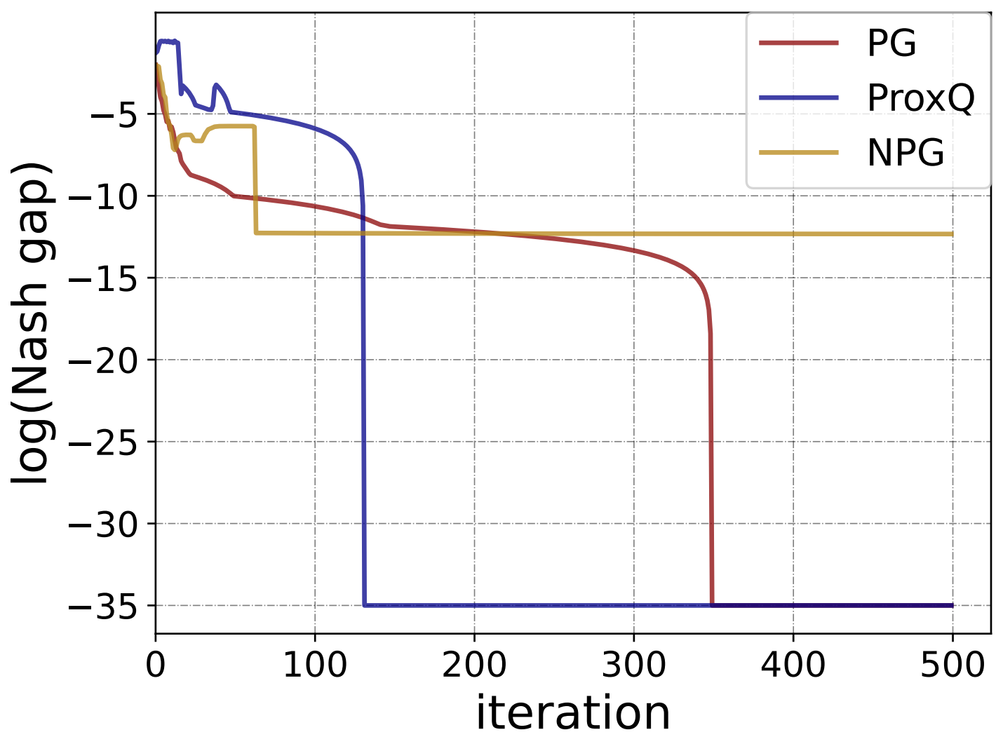
(c) Large LVR, small RG

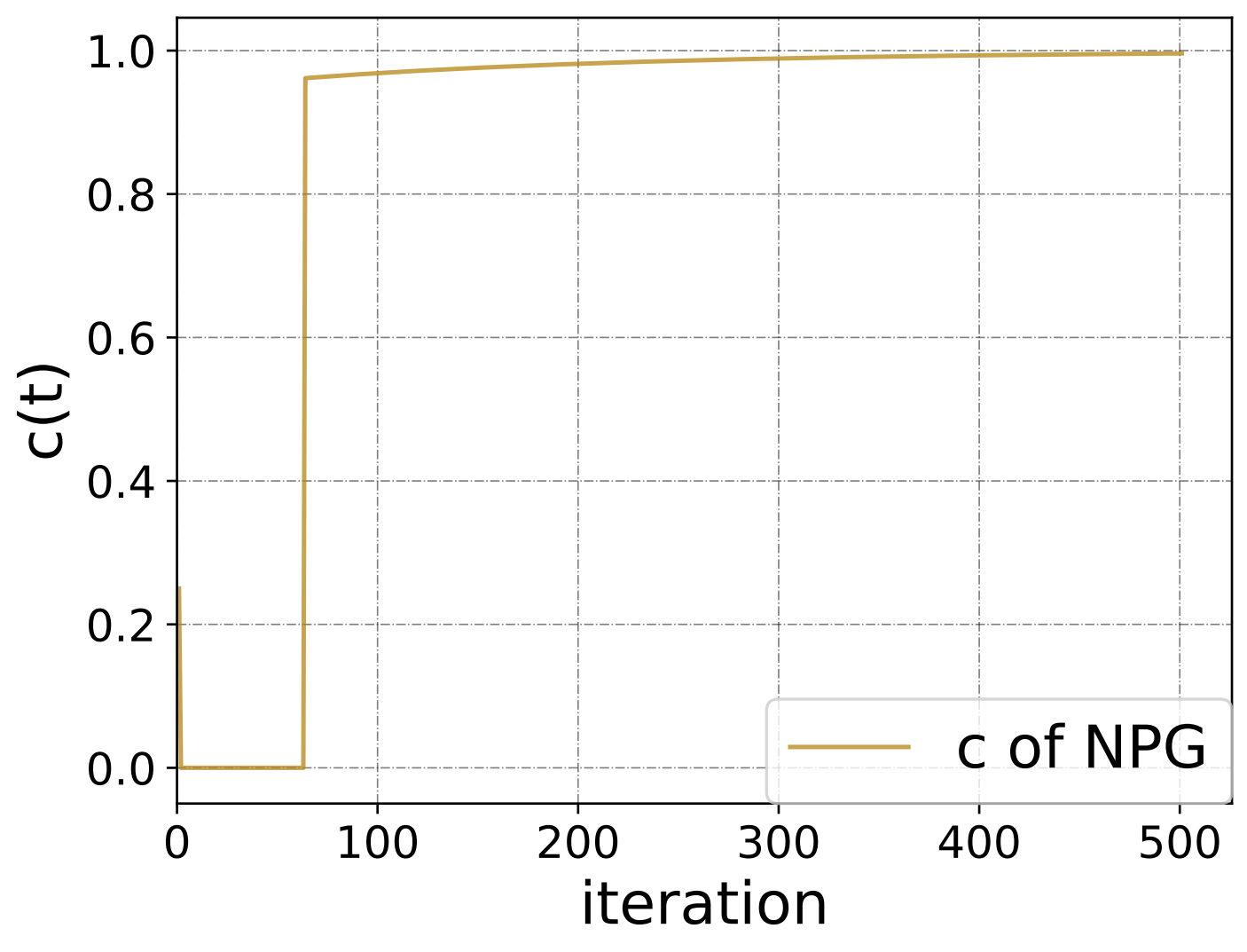
(d) Large LVR, small RG

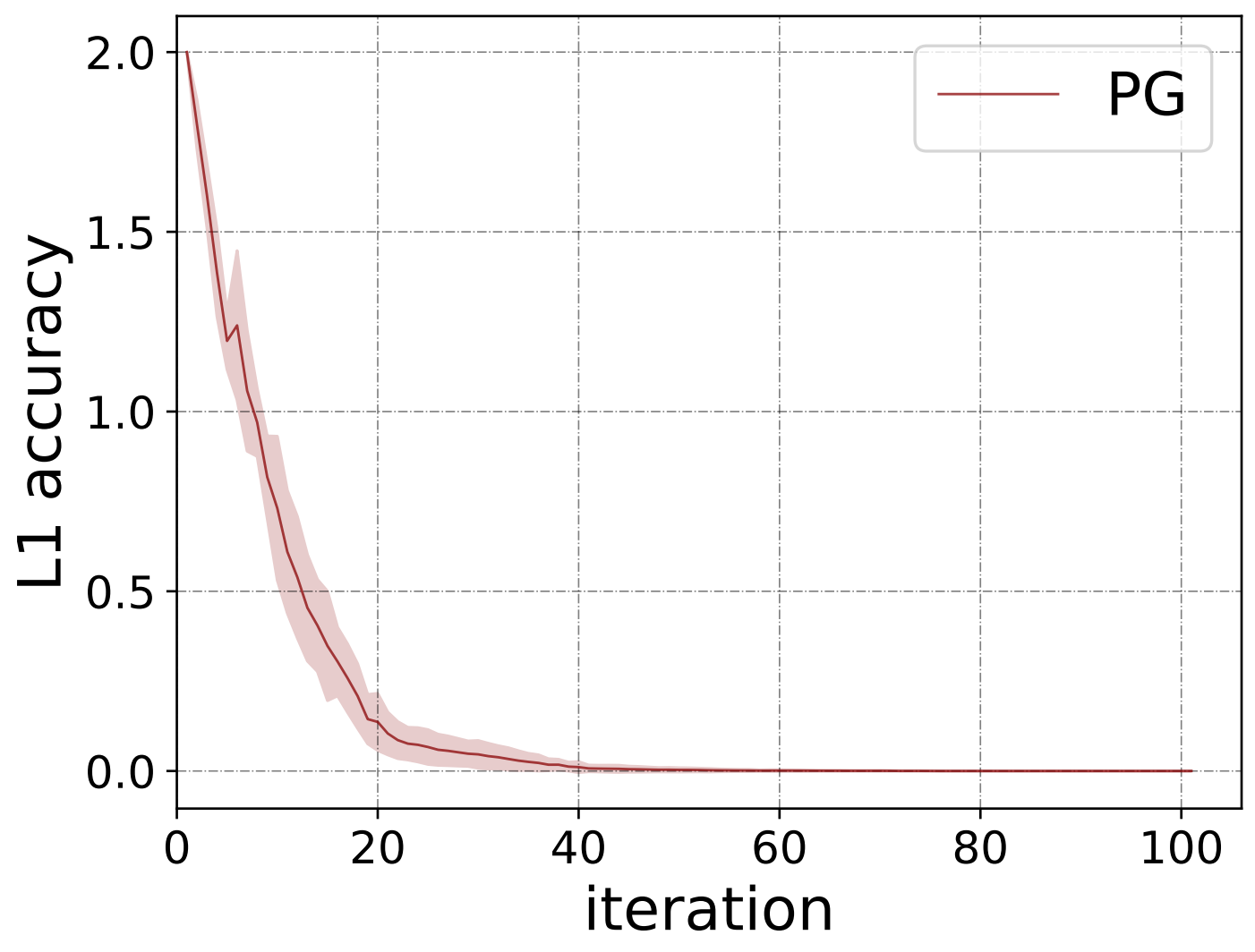
(e) $\ell_{1}$ accuracy

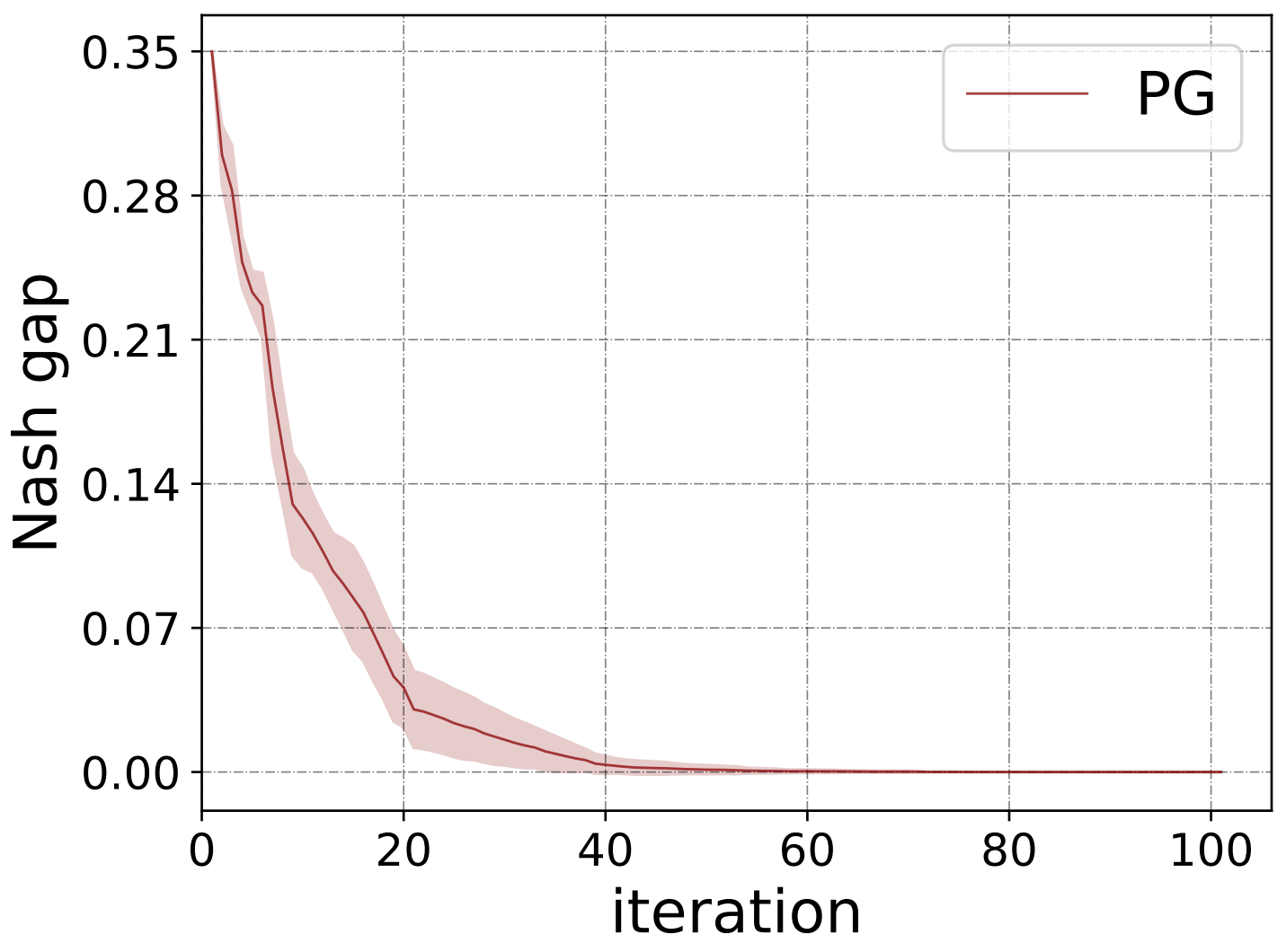
(f) Nash gap

Figure 1: (a)(b)(c)(d) are results for the oracle setting. Since the Nash gap can be as low as $0.0$, we truncate the $\log(\text{Nash gap})$ at $-35$ from below. (d) depicts the change in $c(t)$ of the NPG algorithm for Fig. 1(c). (e) and (f) present the results of Algorithm 2. The solid lines are the means of trajectories over seven random seeds and shaded regions are the standard deviations.

We first illustrate the convergence of the algorithms in the oracle setting. We randomly generate a Markov potential game model with $S=100$ states, and $A_{1}=4$, $A_{2}=3$, $A_{3}=2$ actions for the $N=3$ agents. We choose the largest learning rate. This yields the fastest convergence for each algorithm. The numerical experiments corroborate our theoretical findings in Theorems 1, 3, and 4.

Recall that in the theorems, a small least visited rate (LVR) $(1-\Gamma)$ has a negative impact on the convergence rate. As shown in Fig. 1(a) and 1(b),the small LVR impedes the convergence of all three algorithms. Comparing the theoretical findings of policy gradient and that of proximal-Q and NPG, we note that the complexity of the former is of order $S^{5/2}$ while the latter is of order $S^{3/2}$. This is also verified in Fig. 1(b) and the effect is more significant when LVR is small. In addition, the convergence of NPG depends on the exploration factor $c(t)$. We generate a reward function with a small reward gap (RG) between the optimal action and the second best optimal one, which increases the exploration difficulty and results in a small value of $c(t)$. Despite $c(t)$ nearing 1, with very small RG, NPG updates can become minor, causing the algorithm to get stuck near a Nash equilibrium (Fig. 1(d)). Further discussion is in Appendix A.

We further demonstrate that the proposed sample-based independent policy gradient Algorithm 2 converges to the desired policy in Fig. 1(e) and 1(f), under both the $\ell_{1}$ accuracy, i.e., $\frac{1}{N}\sum_{i=1}^{N}\lVert\pi_{i}^{t}-\pi_{i}^{*}\rVert_{1}$ and Nash gap.

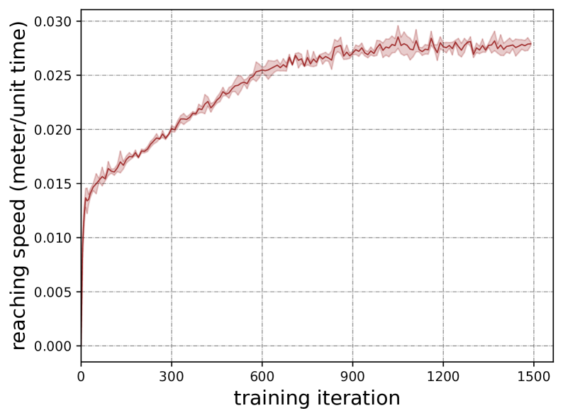
Figure 2: Training process of robot navigation task. The solid line is the mean of trajectories over three random seeds and shaded regions are the standard deviations.

To illustrate the potential of the independent learning scheme in averaged reward MARL, a more complex robot navigation task is conducted. There are two controllers (linear speed controller and angular speed controller) in a robot with each viewed as an agent. The agents gain rewards when the robot is moving toward the target. We implement a practical version of the independent average NPG algorithm with a neural network, which is inspired by Algorithm 1 of Ma et al., (2021), and showcase its performance in Fig. 2.

7 CONCLUSION

In this paper, we study Markov potential games under the average reward criterion and analyze three algorithms, policy gradient ascent, proximal-Q, and NPG under the access to an oracle. We establish time complexity that matches the results in discounted reward settings. We also propose a gradient estimator, which only relies on a single trajectory. The sample-based policy gradient ascent algorithm is shown to converge to a Nash equilibrium, and a sample complexity is provided. We also close several technical gaps in the analysis of policy gradient methods between the discounted and average reward settings.

Acknowledgements

This material is based upon work partially supported by the US Army Contracting Command under W911NF-22-1-0151 and W911NF2120064, US National Science Foundation under CMMI-2038625, and US Office of Naval Research under N00014-21-1-2385.

Appendix A EXPERIMENTAL DETAILS

A.1 Oracle-based Algorithms

We provide more details regarding the numerical experiments described in Section 6. In the oracle setting, when the state set size is greater than the size of the action set, according to Theorem 1, Theorem 3 and Theorem 4, the time complexities for projected policy gradient ascent, proximal-Q and NPG are

$$O\left(\frac{NC_{\Phi}S^{5/2}A_{\max}\kappa_{0}^{2}}{(1-\Gamma)^{2}\epsilon^{2}}\right),O(\frac{NC_{\Phi}S^{3/2}A_{max}\kappa_{0}^{2}}{(1-\Gamma)^{2}\epsilon^{2}}),\mbox{ and }O(\frac{NC_{\Phi}S^{3/2}A_{\max}\kappa_{0}^{2}}{c(1-\Gamma)^{2}\epsilon^{2}}),$$

respectively. Notably, projected policy gradient ascent exhibits an additional $S$ dependency, while NPG has an additional dependency on $\frac{1}{c}$. Meanwhile, a small least visited rate (LVR) $1-\Gamma$ has a negative effect on all algorithms. To illustrate these effects, we conducted simulations on Markov potential games with large state spaces, varying LVR (large or small), and different exploration factors (large or small $c$), as described in the next paragraph.

We randomly generate a cooperative Markov potential game with the following parameters: $S=100$, $A_{1}=4$, $A_{2}=3$, and $A_{3}=2$. To control the LVR $(1-\Gamma)$, the elements of the transition probability matrix $P\in[0,1]^{SA_{1}A_{2}A_{3}\times S}$ are generated as follows. First, each entry is generated using a uniform distribution $\text{Unif}[0,1]$. Then we randomly select half of the states (denoting chosen states by $s^{\prime}$) and generate the probabilities $P(s^{\prime}|s,\mathbf{a})$ for every action profile $\mathbf{a}$ according to a uniform distribution $\text{Unif}[0,0.01]$ (for small LVR), or $\text{Unif}[0,0.1]$ or $\text{Unif}[0,1]$ (for large LVR). Subsequently, each row of the matrix is normalized. To reduce the exploration factor $c$, we generate a reward function with a small reward gap (RG) between the reward of the best action and that of the second best action, thereby increasing exploration difficulty and leading to a smaller $c$. The reward function is identical for all agents. It is randomly generated and denoted as $R\in[0,1]^{SA_{1}A_{2}A_{3}}$. For scenarios with a small RG, we use a uniform distribution $\text{Unif}[0,1]$ for all entries, or set reward $r(s,\mathbf{a}^{\prime})$ to be $0.001$ smaller than $\max_{\mathbf{a}}r(s,\mathbf{a})$. This setup can indeed make $c(t)$ smaller as illustrated in Fig. 1(d). In cases with a large RG, we select an action profile for each state at random and generate rewards according to $\text{Unif}[0.4,1]$, with the remaining entities generated according to $\text{Unif}[0,0.6]$. We observed that a larger learning rate leads to faster convergence, therefore, we chose the largest learning rate.

A.2 Sample-based Algorithm

In the sample-based setting, we run Algorithm 2 for a manually designed Markov potential game with $S=2$, $A_{1}=A_{2}=2$, an action-independent transition probability matrix $P=\begin{pmatrix}0.9&0.1\\ 0.3&0.7\end{pmatrix}$, and a reward function that is identical for each agent. The rewards for states 1 and 2 are $R_{1}=\begin{pmatrix}1&0.2\\ 0.8&0.2\end{pmatrix}$ and $R_{1}=\begin{pmatrix}0.2&1\\ 0.1&0.6\end{pmatrix}$, where columns indicate actions for agent 1, and rows indicate actions for agent 2. To achieve $\alpha=0.01$ and $\delta=0.01$, Theorem 2 suggests a learning rate $\beta\approx\frac{1}{N\kappa_{0}^{2}S^{3/2}A_{\max}}\approx 0.01$ and trajectory length $KN_{2}+N_{1}\approx 10^{8}$. To reduce the number of samples needed, we choose a trajectory length $KN_{2}+N_{1}=51000$ with $N_{1}=1000,N_{2}=50,K=1000$, and reduce the step size every $20$ steps, from initially $0.5$ to eventually $0.0001$, to accommodate inaccurate gradient estimates.

A.3 Robot Navigation Task

We demonstrate the efficacy of average reward MARL by solving a complex robot navigation task for TurtleBot, a two-wheeled mobile robot (Zhou et al.,, 2024; Rengarajan et al., 2022a, ; Rengarajan et al., 2022b, ) in a simulation platform, Gazebo. The navigation task is to guide the robot to any designated target within a 2-meter radius. The state space is defined by a continuous 2-dimensional space representing the distance and relative orientation between the robot and the target. The robot is equipped with two controllers: an angular controller with control effect ranging from -1.5 rad/s to 1.5 rad/s, and a linear velocity controller with control effect ranging from 0 cm/s to 15 cm/s. To model the agents’ control strategy, we implemented two independent agents to manage the angular and linear speeds, following an empirical adaptation of Algorithm 5. The reward function is formulated to be proportional to the product of the distance and the scaled orientation between the robot and the target. Hitting the boundary incurs a penalty of -200, while reaching the target yields a reward of 200. Each trajectory terminates upon collision, achievement of the goal, or after 500 simulation steps have elapsed.

All experiments were conducted on a CPU with an 11th Gen Intel(R) Core(TM) i7-11700 @ 2.50GHz.

Appendix B PROOFS OF SECTION 2

We first explore a sufficient condition for a Markov game to be a potential game. Previous works have studied the sufficient condition for the discounted reward setting (Leonardos et al.,, 2021; Zhang et al., 2021a, ; Narasimha et al.,, 2022). These conditions encompass some important Markov games.

Proposition 2.

Consider a Markov game that is a static potential game $r_{i}(s,\mathbf{a})$ at every state $s\in\mathrm{S}$, i.e., there exists a common potential function $\phi(s,\mathbf{a})$ and an utility function $u_{i}(s,a_{-i})$ for each agent $i$, such that $r_{i}(s,\mathbf{a})=\phi(s,\textbf{a})+u_{i}(s,a_{-i})$. If one of the following conditions is satisfied, then the Markov game is an average reward Markov potential game:

1. The transition probabilities do not depend on the action $\mathbf{a}$ taken, i.e., $P(s^{\prime}|s,\mathbf{a})=P(s^{\prime}|s)$ for all $\mathbf{a}$.

2. For every agent $i$, there exist a constant $c_{i}$ such that $\overline{u}^{\pi_{-i}}_{i}(s):=\sum_{a_{-i}}(\Pi_{j\neq i}\pi_{j}(a_{j}|s))u_{i}(s,a_{-j})$ satisfies $\nabla_{\pi_{i}(\cdot|s)}\langle\nu^{\pi},\overline{u}^{\pi_{-i}}_{i}\rangle=c_{i}\mathbf{1}_{A_{i}}$ for every state $s$ and policy $\pi$.

Proof.

Let $\overline{\phi}^{\pi}(s):=\sum_{\mathbf{a}}\pi(\mathbf{a}|s)\phi(s,\mathbf{a})$. $\rho_{i}^{\pi}=\langle\nu^{\pi},\overline{\phi}^{\pi}+\overline{u}_{i}^{\pi_{-i}}\rangle$. If condition 1 is satisfied, $\nu^{\pi}\equiv\nu$, then $\langle\nu,\overline{\phi}^{\pi}\rangle$ is the potential function.

If condition 2 is satisfied, $\rho_{i}^{\pi}=\langle\nu^{\pi},\overline{\phi}^{\pi}\rangle+\langle\nu^{\pi},\overline{u}_{i}^{\pi_{-i}}\rangle$. With the interpolation of differential function, for any policies $\pi_{i},\pi_{i}^{\prime}$ and $\pi_{-i}$, there exist a constant $a\in[0,1]$, $\pi_{i}^{*}=\pi_{i}+a(\pi_{i}^{\prime}-\pi_{i})$, such that $\rho^{\pi_{i},\pi_{-i}}-\rho_{i}^{\pi_{i}^{\prime},\pi_{-i}}=\langle\nu^{\pi},\overline{\phi}^{\pi}\rangle-\langle\nu^{\pi_{i}^{\prime},\pi_{-i}},\overline{\phi}^{\pi_{i}^{\prime},\pi_{-i}}\rangle+\langle\pi_{i}-\pi_{i}^{\prime},\nabla_{\pi_{i}(\cdot|s)}\langle\nu^{\pi_{i}^{*},\pi_{-i}},\overline{u}^{\pi_{-i}}_{i}\rangle\rangle=\langle\nu^{\pi},\overline{\phi}^{\pi}\rangle-\langle\nu^{\pi_{i}^{\prime},\pi_{-i}},\overline{\phi}^{\pi_{i}^{\prime},\pi_{-i}}\rangle+\langle\pi_{i}-\pi_{i}^{\prime},c_{i}\mathbf{1}_{A_{i}}\rangle=\langle\nu^{\pi},\overline{\phi}^{\pi}\rangle-\langle\nu^{\pi_{i}^{\prime},\pi_{-i}},\overline{\phi}^{\pi_{i}^{\prime},\pi_{-i}}\rangle$. Therefore, $\langle\nu^{\pi},\overline{\phi}^{\pi}\rangle$ is the potential function. ∎

Remark

A fully cooperative game, where all agents have the same reward function $r_{i}\equiv r$, is an important special case of a Markov potential game. It satisfies Condition 2 in Proposition 2 with $u_{i}\equiv 0$, while the lake usage problem (Dechert and O’Donnell,, 2006) satisfies Condition 1.

Lemma 9 (Restatement of Lemma 1).

$$\rho_{i}^{\hat{\pi}_{j},\pi_{-j}}-\rho_{i}^{\tilde{\pi}_{j},\pi_{-j}} =\mathbb{E}_{s\sim\nu^{\hat{\pi}_{j},\pi_{-j}}}[\langle\overline{Q}_{j:i}^{\tilde{\pi}_{j},\pi_{-j}}(s,\cdot),\hat{\pi}_{j}(\cdot|s)-\tilde{\pi}_{j}(\cdot|s)\rangle_{\mathcal{A}_{j}}]$$ (5)

$$=\mathbb{E}_{s\sim\nu^{\hat{\pi}_{j},\pi_{-j}}}\sum_{a_{j}}\hat{\pi}_{j}(a_{j}|s)\overline{A}_{j:i}^{\tilde{\pi}_{j},\pi_{-j}}(s,a_{j}).$$

Proof.

$$\rho_{i}^{\hat{\pi}_{j},\pi_{-j}}-\rho_{i}^{\tilde{\pi}_{j},\pi_{-j}}$$

$$= \rho_{i}^{\hat{\pi}_{j},\pi_{-j}}-\rho_{i}^{\tilde{\pi}_{j},\pi_{-j}}+\mathbb{E}_{s^{\prime}\sim\nu^{\hat{\pi}_{j},\pi_{-j}}}[V_{i}^{\tilde{\pi}_{j},\pi_{-j}}(s^{\prime})]-\mathbb{E}_{s\sim\nu^{\hat{\pi}_{j},\pi_{-j}}}[V_{i}^{\tilde{\pi}_{j},\pi_{-j}}(s)]$$

$$= \mathbb{E}_{s\sim\nu^{\hat{\pi}_{j},\pi_{-j}},\textbf{a}\sim(\hat{\pi}_{j},\pi_{-j})}[r_{i}(s,a)-\rho_{i}^{\tilde{\pi}_{j},\pi_{-j}}+\mathbb{E}_{s^{\prime}\sim P(\cdot|s,a)}[V_{i}^{\tilde{\pi}_{j},\pi_{-j}}(s^{\prime})]-V_{i}^{\tilde{\pi}_{j},\pi_{-j}}(s)]$$

$$= \mathbb{E}_{s\sim\nu^{\hat{\pi}_{j},\pi_{-j}},\textbf{a}\sim(\hat{\pi}_{j},\pi_{-j})}[Q_{i}^{\tilde{\pi}_{j},\pi_{-j}}(s,\textbf{a})-\langle\overline{Q}_{j;i}^{\tilde{\pi}_{j},\pi_{-j}}(\cdot,s),\tilde{\pi}_{j}(\cdot|s)\rangle_{\mathcal{A}_{j}}]$$

$$= \mathbb{E}_{s\sim\nu^{\hat{\pi}_{j},\pi_{-j}}}[\mathbb{E}_{a_{j}\sim\hat{\pi}_{i}}\overline{Q}_{j;i}^{\tilde{\pi}_{j},\pi_{-j}}(s,a_{j})-\langle\overline{Q}_{j;i}^{\tilde{\pi}_{j},\pi_{-j}}(\cdot,s),\tilde{\pi}_{j}(\cdot|s)\rangle_{\mathcal{A}_{j}}]$$

$$= \mathbb{E}_{s\sim\nu^{\hat{\pi}_{j},\pi_{-j}}}[\langle\overline{Q}_{j;i}^{\tilde{\pi}_{j},\pi_{-j}}(s,\cdot),\hat{\pi}_{j}(\cdot|s)-\tilde{\pi}_{j}(\cdot|s)\rangle_{\mathcal{A}_{j}}]$$

$$= \mathbb{E}_{s\sim\nu^{\hat{\pi}_{j},\pi_{-j}}}[\sum_{a_{j}}\overline{Q}_{j;i}^{\tilde{\pi}_{j},\pi_{-j}}(s,a_{j})\hat{\pi}_{j}(a_{j}|s)-V_{i}^{\tilde{\pi}_{j},\pi_{-j}}(s)]$$

$$= \mathbb{E}_{s\sim\nu^{\hat{\pi}_{j},\pi_{-j}}}[\sum_{a_{j}}\left(\overline{Q}_{j;i}^{\tilde{\pi}_{j},\pi_{-j}}(s,a_{j})-V_{i}^{\tilde{\pi}_{j},\pi_{-j}}(s)\right)\hat{\pi}_{j}(a_{j}|s)]$$

$$= \mathbb{E}_{s\sim\nu^{\hat{\pi}_{j},\pi_{-j}}}[\sum_{a_{j}}\hat{\pi}_{j}(a_{j}|s)\overline{A}_{j;i}^{\tilde{\pi}_{j},\pi_{-j}}(s,a_{j})].$$

∎

Lemma 10 (Restatement of Lemma 2).

$$\frac{\partial\rho_{i}^{\pi}}{\partial\pi_{j}(a_{j}|s)}=\overline{Q}_{j;i}^{\pi}(s,a_{j})\nu^{\pi}(s),\ \frac{\partial\Phi(\pi)}{\partial\pi_{j}(a_{j}|s)}=\overline{Q}_{j}^{\pi}(s,a_{j})\nu^{\pi}(s)$$

Proof.

Recall that $\overline{Q}_{j:i}^{\pi}(s,a_{j})=\underset{a_{-j}\in\mathcal{A}_{-j}}{\sum}\pi_{-j}(a_{-j}|s)Q^{\pi}_{i}(s,a_{j},a_{-j})=\underset{a_{-j}\in\mathcal{A}_{-j}}{\sum}\pi_{-j}(a_{-j}|s)(r(s,\textbf{a})-\rho^{\pi}_{i}+\mathbb{E}_{s^{\prime}\sim P(\cdot|s,a)}V^{\pi}_{i}(s^{\prime}))$. Therefore, $V_{i}^{\pi}(s)=\sum_{a_{j}}\pi_{j}(a_{j}|s)\overline{Q}_{j;i}^{\pi}(s,a_{j})$. Differentiating with respect to $\pi_{j}$:

$$\frac{\partial V_{i}^{\pi}(s)}{\partial\pi_{j}} =\frac{\partial}{\partial\pi_{j}}\sum_{a_{j}}\pi_{j}(a_{j}|s)\overline{Q}_{j;i}^{\pi}(s,a_{j})$$

$$=\sum_{a_{j}}\frac{\partial\pi_{j}(a_{j}|s)}{\partial\pi_{j}}\overline{Q}_{j;i}^{\pi}(s,a_{j})+\sum_{a_{j}}\pi_{j}(a_{j}|s)\frac{\partial\overline{Q}_{j;i}^{\pi}(s,a_{j})}{\partial\pi_{j}}$$

$$=\sum_{a_{j}}\frac{\partial\pi_{j}(a_{j}|s)}{\partial\pi_{j}}\overline{Q}_{j;i}^{\pi}(s,a_{j})+\sum_{a_{j}}\pi_{j}(a_{j}|s)\frac{\partial}{\partial\pi_{j}}(r_{i}^{\pi_{-j}}(s,a_{j})-\rho_{i}^{\pi}+\mathbb{E}_{s^{\prime}\sim P(\cdot|s,a_{j},a_{-j}),a_{-j}\sim\pi_{-j}(\cdot|s)}V^{\pi}_{i}(s^{\prime}))$$

$$=\sum_{a_{j}}\frac{\partial\pi_{j}(a_{j}|s)}{\partial\pi_{j}}\overline{Q}_{j;i}^{\pi}(s,a_{j})-\frac{\partial\rho_{i}^{\pi}}{\partial\pi_{j}}+\mathbb{E}_{s^{\prime}\sim P(\cdot|s,a),\textbf{a}\sim\pi(\cdot|s)}\frac{\partial V^{\pi}_{i}(s^{\prime})}{\partial\pi_{j}}.$$

Multiplying each side with $\nu^{\pi}(s)$, taking the summation over $s$, with the definition of stationary distribution $\mathbb{E}_{s\sim\nu^{\pi},s^{\prime}\sim P(\cdot|s,a),a\sim\pi(\cdot|s)}=\mathbb{E}_{s^{\prime}\sim\nu^{\pi}}$, we obtain:

$$\sum_{s}\nu^{\pi}(s)\frac{\partial V_{i}^{\pi}(s)}{\partial\pi_{j}}= \sum_{s}\nu^{\pi}(s)\sum_{a_{j}}\frac{\partial\pi_{j}(a_{j}|s)}{\partial\pi_{j}}\overline{Q}_{j;i}^{\pi}(s,a_{j})-\frac{\partial\rho_{i}^{\pi}}{\partial\pi_{j}}+\mathbb{E}_{s^{\prime}\sim\nu^{\pi}}\frac{\partial V^{\pi}_{i}(s^{\prime})}{\partial\pi_{j}},$$

$$0= \sum_{s}\nu^{\pi}(s)\sum_{a_{j}}\frac{\partial\pi_{j}(a_{j}|s)}{\partial\pi_{j}}\overline{Q}_{j;i}^{\pi}(s,a_{j})-\frac{\partial\rho_{i}^{\pi}}{\partial\pi_{j}},$$

$$\frac{\partial\rho_{i}^{\pi}}{\partial\pi_{j}}= \sum_{s}\nu^{\pi}(s)\sum_{a_{j}}\overrightarrow{\mathbf{e}}(s,a_{j})\overline{Q}_{j;i}^{\pi}(s,a_{j}).$$

By the definition of the potential function, it can be noted that $\frac{\partial\Phi(\pi)}{\partial\pi_{j}(a_{j}|s)}=\frac{\partial\rho_{j}^{\pi}}{\partial\pi_{j}(a_{j}|s)}=\overline{Q}_{j}^{\pi}(s,a_{j})\nu^{\pi}(s)$. ∎

Lemma 11 (Kale,, 2013, Theorem 3.1, equation (4)).

Given a Markov chain with transition probability matrix $P\in\mathbb{R}^{S\times S}$, let $\nu$ be its stationary distribution. For any $s,s^{\prime}\in\mathcal{S}$, we have:

$$|\frac{P^{t}(s^{\prime}|s)}{\nu(s^{\prime})}-1|\leq\frac{\lambda_{2}(P)^{t}}{\sqrt{\nu(s)\nu(s^{\prime})}}.$$

Lemma 12 (Restatement of Lemma 3).

There exist constants $C_{p}:=\min\{\sqrt{\frac{S}{1-\Gamma}},\frac{1}{1-\Gamma}\}$ and $\varrho:=1-\frac{1}{\kappa_{0}}$ such that for any policy $\pi$:

$$sup_{s}\lVert(P^{\pi})^{t}(\cdot|s_{0}=s)-\nu^{\pi}\rVert_{1}\leq C_{p}\varrho^{t},\forall\ t>0.$$

Proof.

For any policy $\pi\in\Pi$, $|\frac{(P^{\pi})^{t}(s^{\prime}|s)}{\nu^{\pi}(s^{\prime})}-1|\leq\frac{\lambda_{2}(P^{\pi})^{t}}{\sqrt{\nu^{\pi}(s)\nu^{\pi}(s^{\prime})}}$ by Lemma 11. Then $\sum_{s^{\prime}}|(P^{\pi})^{t}(s^{\prime}|s)-\nu^{\pi}(s^{\prime})|\leq\lambda_{2}(P^{\pi})^{t}\sum_{s^{\prime}}\sqrt{\frac{\nu^{\pi}(s^{\prime})}{\nu^{\pi}(s)}}\leq\left(1-(\frac{1}{1-\lambda_{2}(P^{\pi})})^{-1}\right)^{t}\sum_{s^{\prime}}\sqrt{\nu^{\pi}(s^{\prime})}\frac{1}{\sqrt{1-\Gamma}}\leq(1-\frac{1}{\kappa_{0}})^{t}\sqrt{\frac{S}{1-\Gamma}}$.

Similarly, recall $|\frac{(P^{\pi})^{t}(s^{\prime}|s)}{\nu^{\pi}(s^{\prime})}-1|\leq\frac{\lambda_{2}(P^{\pi})^{t}}{\sqrt{\nu^{\pi}(s)\nu^{\pi}(s^{\prime})}}\leq\frac{\lambda_{2}(P^{\pi})^{t}}{1-\Gamma}$, then $\sum_{s^{\prime}}|(P^{\pi})^{t}(s^{\prime}|s)-\nu^{\pi}(s^{\prime})|\leq\frac{\lambda_{2}(P^{\pi})^{t}}{1-\Gamma}=(1-\frac{1}{\kappa_{0}})^{2}\frac{1}{1-\Gamma}$. ∎

Proposition 3.

For any policy $\pi$ and any agent $i$, the differential Q function has a bounded $\ell_{\infty}$ norm:

$$\lVert Q^{\pi}_{i}\rVert_{\infty}\leq C_{p}\kappa_{0}.$$

Proof.

For any $s,\mathbf{a}$ and joint policy $\pi$, $|Q^{\pi}_{i}(s,\mathbf{a})|=|\mathbb{E}_{\pi}[\sum_{t=0}^{\infty}(r_{i}(s^{t},\mathbf{a}^{t})-\rho_{i}^{\pi})|s^{0}=s,\mathbf{a}^{0}=\mathbf{a}]|\leq 1+|\mathbb{E}_{s^{\prime}\sim P(\cdot|s,\mathbf{a})}\sum_{t=1}^{\infty}\langle(P^{\pi})^{t}(\cdot|s^{\prime})-\nu^{\pi},r^{\pi}\rangle|\leq 1+\sum_{t=1}^{\infty}C_{p}\varrho^{t}=1+\frac{C_{p}\varrho}{1-\varrho}=1+C_{p}(\kappa_{0}-1)<C_{p}\kappa_{0}$. ∎

Appendix C PROOFS OF SECTION 3

C.1 Auxiliary Lemmas

Lemma 13 (Leonardos et al.,, 2021, Lemma 4.1).

Let $\pi=(\pi_{1},\pi_{2},...,\pi_{N})$ be the policy profile for all agents and let $\pi^{\prime}=\pi+\lambda\nabla_{\pi}\Phi(\pi)$ be the result from a gradient step on the potential function with learning rate $\lambda>0$. Then

$$\textnormal{Proj}_{\Pi_{1}\times...\times\Pi_{N}}(\pi^{\prime})=(\textnormal{Proj}_{\Pi_{1}}(\pi_{1}^{\prime}),...,\textnormal{Proj}_{\Pi_{N}}(\pi_{N}^{\prime})).$$

Lemma 14 (Agarwal et al.,, 2021, Proposition B.1).

Let $f(\pi)$ be an $l$-smooth function. Define the gradient mapping $G(\pi):=\frac{1}{\beta}(\textnormal{Proj}_{\Pi}(\pi+\beta\nabla_{\pi}f(\pi))-\pi)$. Then the update rule for the projected gradient is $\pi^{+}=\pi+\beta G(\pi)$. If $\lVert G(\pi)\rVert_{2}\leq\epsilon$, then

$$\underset{\pi^{+}+\delta\in\Pi,\lVert\delta\rVert_{2}\leq 1}{\max}\delta^{T}\nabla_{\pi}f(\pi^{+})\leq\epsilon(\beta l+1).$$

There is a typographical mistake in proposition B.1 of Agarwal et al., (2021); the underlying max should be taken on $\pi^{+}+\delta\in\Pi$ instead of $\pi+\delta\in\Pi$.

Lemma 15 (Bubeck et al.,, 2015, Lemma 3.6).

Let $f$ be an $l$-smooth function over a convex domain $C$. Let $x\in C$, $x^{+}=\textnormal{Proj}_{C}(x-\beta\nabla f(x))$. Then :

$$f(x^{+})-f(x)\leq(\frac{l}{2}-\frac{1}{\beta})\lVert x-x^{+}\rVert_{2}^{2}.$$

Lemma 16.

Assume function $f(\cdot)$ is $l$-smooth over a convex set $C$. Let $x^{+}:=P_{C}(x-\beta g)$ with $x\in C$. Then

$$f(x^{+})-f(x)\leq(\frac{3l}{4}-\frac{1}{\beta})\lVert x-x^{+}\rVert_{2}^{2}+\frac{1}{l}\lVert\nabla_{x}f(x)-g\rVert_{2}^{2}.$$

Proof.

$$f(x^{+})-f(x)\leq \langle\nabla f(x),x^{+}-x\rangle+\frac{l}{2}\lVert x^{+}-x\rVert_{2}^{2}$$

$$= \langle g,x^{+}-x\rangle+\frac{l}{2}\lVert x^{+}-x\rVert_{2}^{2}+\langle\nabla f(x)-g,x^{+}-x\rangle$$

$$\overset{(a)}{\leq} -\frac{1}{\beta}\lVert x-x^{+}\rVert_{2}^{2}+\frac{l}{2}\lVert x^{+}-x\rVert_{2}^{2}+\frac{1}{2}(\frac{2}{l}\lVert\nabla_{x}f(x)-\hat{\nabla}_{x}f(x)\rVert_{2}^{2}+\frac{l}{2}\lVert x^{+}-x\rVert_{2}^{2})$$

$$= (\frac{3l}{4}-\frac{1}{\beta})\lVert x-x^{+}\rVert_{2}^{2}+\frac{1}{l}\lVert\nabla_{x}f(x)-g\rVert_{2}^{2}.$$

We use the property of projection in (a) $\langle x^{+}-(x-\beta g),x^{+}-x\rangle\leq 0$ and $\langle x,y\rangle\leq\frac{\frac{1}{a}\lVert x\rVert_{2}^{2}+a\lVert y\rVert_{2}^{2}}{2}$ for any positive constant $a$. ∎

C.2 Proofs of Lemma 4 and Theorem 1

Lemma 17 (Restatement of Lemma 4).

Denote $A_{\max}:=\max_{i}A_{i}$, $L:=\kappa_{0}^{2}S^{3/2}A_{\max}+\kappa_{0}\sqrt{S}A_{\max}$, and $L_{\Phi}:=N(\kappa_{0}^{2}S^{3/2}A_{\max}+\kappa_{0}(SA_{\max}+2A_{\max})+A_{\max})$.

(a) For any i, and $\pi_{-i}\in\Pi_{-i}$, the average value $\rho_{i}^{\pi}$ is $\kappa_{0}^{2}S^{3/2}A_{i}+\kappa_{0}\sqrt{S}A_{i}$-smooth with respect to policy $\pi_{i}$. Moreover, for any $i$, $\rho_{i}^{\pi}$ is $L$-smooth with respect to policy $\pi_{i}$, i.e. $\lVert\nabla_{\pi_{i}}\rho_{i}^{\pi_{i},\pi_{-i}}-\nabla_{\pi_{i}}\rho_{i}^{\pi_{i}^{\prime},\pi_{-i}}\rVert_{2}\leq L\lVert\pi_{i}-\pi_{i}^{\prime}\rVert_{2}$ for $\forall\ i,\ and\ \pi_{i},\pi_{i}^{\prime}\in\Pi_{i}$.

(b) The potential function $\Phi(\pi)$ is $L_{\Phi}$-smooth with respect to policy profile $\pi$, i.e. $\lVert\nabla\Phi(\pi)-\nabla\Phi(\pi^{\prime})\rVert_{2}\leq L_{\Phi}\lVert\pi-\pi^{\prime}\rVert_{2}$ for $\forall\ \pi,\pi^{\prime}\in\Pi$.

Proof.

By the potential function property $\Phi(\pi_{i},\pi_{-i})-\Phi(\pi_{i}^{\prime},\pi_{-i})=\rho_{i}^{\pi_{i},\pi_{-i}}-\rho_{i}^{\pi_{i}^{\prime},\pi_{-i}}$, $\frac{\partial}{\partial\pi_{i}}\Phi(\pi_{i},\pi_{-i})=\frac{\partial}{\partial\pi_{i}}\rho_{i}^{\pi_{i},\pi_{-i}}$, and $\nabla_{\pi}\Phi=(\frac{\partial\rho^{\pi}_{1}}{\partial\pi_{1}},...,\frac{\partial\rho^{\pi}_{N}}{\partial\pi_{N}})^{T}$. To show the smoothness,

$$\lVert\nabla_{\pi}\Phi(\pi)-\nabla_{\pi}\Phi(\pi^{\prime})\rVert_{2}^{2}$$

$$= \sum_{i=1}^{N}\lVert\nabla_{\pi_{i}}\Phi(\pi)-\nabla_{\pi_{i}}\Phi(\pi^{\prime})\rVert_{2}^{2}$$

$$= \sum_{i=1}^{N}\lVert\nabla_{\pi_{i}}\Phi(\pi)-\nabla_{\pi_{i}}\Phi(\pi_{1}^{\prime},\pi_{2\sim N})+\nabla_{\pi_{i}}\Phi(\pi_{1}^{\prime},\pi_{2\sim N})-\nabla_{\pi_{i}}\Phi(\pi_{1,2}^{\prime},\pi_{3\sim N})+\ldots$$

$$+\nabla_{\pi_{i}}\Phi(\pi_{1\sim(N-1)},\pi^{\prime}_{N})-\nabla_{\pi_{i}}\Phi(\pi^{\prime})\rVert_{2}^{2}$$

$$\leq \sum_{i=1}^{N}\sum_{j=1}^{N}N\lVert\nabla_{\pi_{i}}\Phi(\pi_{1\sim j-1},\pi^{\prime}_{j\sim N})-\nabla_{\pi_{i}}\Phi(\pi_{1\sim j},\pi^{\prime}_{j+1\sim N})\rVert_{2}^{2}$$

$$= \sum_{i=1}^{N}\sum_{j=1}^{N}N\lVert\frac{\partial\rho_{i}^{\pi_{1\sim j-1},\pi^{\prime}_{j\sim N}}}{\partial\pi_{i}}-\frac{\partial\rho_{i}^{\pi_{1\sim j},\pi^{\prime}_{j+1\sim N}}}{\partial\pi_{i}}\rVert_{2}^{2}.$$

If we can show $\frac{\partial\rho_{i}^{\pi}}{\partial\pi_{i}}$ is $\frac{L_{\Phi}}{N}$-lipschitz for any $\pi_{j}$ within $\Pi_{j}$, the above inequality implies that $\lVert\nabla_{\pi}\Phi(\pi)-\nabla_{\pi}\Phi(\pi^{\prime})\rVert_{2}^{2}\leq\sum_{i=1}^{N}\sum_{j=1}^{N}\frac{L_{\Phi}^{2}}{N}\lVert\pi_{j}-\pi_{j}^{\prime}\rVert_{2}^{2}=L_{\Phi}^{2}\lVert\pi-\pi^{\prime}\rVert_{2}^{2}$. In the following proof, we will fix $i$ and denote $\rho=\rho_{i}$.

Define $\rho(\epsilon)=\rho_{i}^{\pi_{i}+\epsilon u_{i},\pi_{-i}}$ and $\rho(\tau,\epsilon)=\rho_{i}^{\pi_{i}+\epsilon u_{i},\pi_{j}+\tau u_{j},\pi_{-ij}}$. We wish to show that $|\frac{d^{2}\rho}{d\epsilon^{2}}|\leq L$, $|\frac{d^{2}\rho}{d\epsilon d\tau}|\leq\frac{L_{\Phi}}{N}$ for any $u_{i},u_{j}$, and any $\epsilon,\tau\in\mathbb{R}$ such that $\pi_{i}+\epsilon u_{i}\in\Pi_{i}$, $\lVert u_{i}\rVert_{2}\leq 1$, $\pi_{j}+\tau u_{j}\in\Pi_{j}$, $\lVert u_{j}\rVert_{2}\leq 1$ and any $\pi\in\Pi$. Note that $\sum_{a_{i}}u_{i}(a_{i}|s)=0$, $\sum_{a_{j}}u_{j}(a_{j}|s)=0$ for any $s$.

We first note that the unit eigenvector $X(\epsilon)$ of the perturbed square matrix $P^{\pi}+\epsilon P^{u_{i}}$ corresponding to the simple eigenvalue $1$ is an analytic function Kazdan, (1995). Recall that for any $\epsilon$, $X(\epsilon)=c\nu^{\pi_{i}+\epsilon u_{i},\pi_{-i}}$ for some constant $c\neq 0$, thus $\sum_{s\in\mathcal{S}}X_{s}(\epsilon)\neq 0$. $\nu^{\pi_{i}+\epsilon u_{i},\pi_{-i}}=(\sum_{s}X_{s}(\epsilon))^{-1}X(\epsilon)$ is therefore analytic, which guarantees the existence of directional derivatives of both $\nu^{\pi_{i}+\epsilon u_{i},\pi_{-i}}$ and $\rho^{\epsilon}$. Then by Garrett, (2005), $\nu^{\epsilon,\tau}=\nu^{\pi_{i}+\epsilon u_{i},\pi_{j}+\tau u_{j},\pi_{-ij}}$ is jointly analytic, and thus $\frac{d^{2}\nu^{\pi_{i}+\epsilon u_{i},\pi_{j}+\tau u_{j},\pi_{-ij}}}{d\epsilon d\tau}$ and $\frac{d^{2}\rho}{d\epsilon d\tau}$ exist.

We first show $|\frac{d^{2}\rho}{d\epsilon^{2}}|\leq L$. Since $\rho(\epsilon)=\sum_{s,\textbf{a}}\nu^{\pi}(s)\pi(\textbf{a}|s)r(s,\textbf{a})=\sum_{s,a_{i}}\nu^{\pi_{i}+\epsilon u_{i},\pi_{-i}}(s)(\pi_{i}(a_{i}|s)+\epsilon u_{i}(a_{i}|s))r^{\pi_{-i}}(s,a_{i})$, we have

$$\frac{d\rho(\epsilon)}{d\epsilon} =\sum_{s,a_{i}}\nu^{\pi_{i}+\epsilon u_{i},\pi_{-i}}(s)u_{i}(a_{i}|s)r^{\pi_{-i}}(s,a_{i})+\sum_{s,a_{i}}\frac{d\nu^{\pi_{i}+\epsilon u_{i},\pi_{-i}}(s)}{d\epsilon}(\pi_{i}(a_{i}|s)+\epsilon u_{i}(a_{i}|s))r^{\pi_{-i}}(s,a_{i}),$$ (6)

$$\frac{d^{2}\rho(\epsilon)}{d\epsilon^{2}} =2\sum_{s,a_{i}}\frac{d\nu^{\pi_{i}+\epsilon u_{i},\pi_{-i}}(s)}{d\epsilon}u_{i}(a_{i}|s)r^{\pi_{-i}}(s,a_{i})+\sum_{s,a_{i}}\frac{d^{2}\nu^{\pi_{i}+\epsilon u_{i},\pi_{-i}}(s)}{d\epsilon^{2}}(\pi_{i}(a_{i}|s)+\epsilon u_{i}(a_{i}|s))r^{\pi_{-i}}(s,a_{i}).$$

Since the stationary distribution satisfies $\nu^{\pi_{i}+\epsilon u_{i},\pi_{-i}}\overrightarrow{\mathbf{1}}\equiv 1$, we have $\frac{d\nu^{\pi_{i}+\epsilon u_{i},\pi_{-i}}}{d\epsilon}\overrightarrow{\mathbf{1}}=0$ and $\frac{d^{2}\nu^{\pi_{i}+\epsilon u_{i},\pi_{-i}}}{d\epsilon^{2}}\overrightarrow{\mathbf{1}}=0$. In other words, $\frac{d\nu^{\pi_{i}+\epsilon u_{i},\pi_{-i}}}{d\epsilon}$ and $\frac{d^{2}\nu^{\pi_{i}+\epsilon u_{i},\pi_{-i}}}{d\epsilon^{2}}$ are orthogonal to $\overrightarrow{\mathbf{1}}$. Taking derivatives on both sides of $\nu^{\pi_{i}+\epsilon u_{i},\pi_{-i}}=\nu^{\pi_{i}+\epsilon u_{i},\pi_{-i}}P^{\pi_{i}+\epsilon u_{i},\pi_{-i}}$ gives

$$\frac{d\nu^{\pi_{i}+\epsilon u_{i},\pi_{-i}}}{d\epsilon}=\nu^{\pi_{i}+\epsilon u_{i},\pi_{-i}}\frac{dP^{\pi_{i}+\epsilon u_{i},\pi_{-i}}}{d\epsilon}+\frac{d\nu^{\pi_{i}+\epsilon u_{i},\pi_{-i}}}{d\epsilon}P^{\pi_{i}+\epsilon u_{i},\pi_{-i}},$$ (7)

$$\frac{d^{2}\nu^{\pi_{i}+\epsilon u_{i},\pi_{-i}}}{d\epsilon^{2}}=\nu^{\pi_{i}+\epsilon u_{i},\pi_{-i}}\frac{d^{2}P^{\pi_{i}+\epsilon u_{i},\pi_{-i}}}{d\epsilon^{2}}+2\frac{d\nu^{\pi_{i}+\epsilon u_{i},\pi_{-i}}}{d\epsilon}\frac{dP^{\pi_{i}+\epsilon u_{i},\pi_{-i}}}{d\epsilon}+\frac{d^{2}\nu^{\pi_{i}+\epsilon u_{i},\pi_{-i}}}{d\epsilon^{2}}P^{\pi_{i}+\epsilon u_{i},\pi_{-i}}.$$

By Definition 4 and the fact that $\frac{d\nu^{\pi_{i}+\epsilon u_{i},\pi_{-i}}}{d\epsilon}$ is orthogonal to the all-1 vector $\mathbf{1}$,

$$\lVert\frac{d\nu^{\pi_{i}+\epsilon u_{i},\pi_{-i}}}{d\epsilon}\rVert_{2}\leq\lVert\nu^{\pi_{i}+\epsilon u_{i},\pi_{-i}}\frac{dP^{\pi_{i}+\epsilon u_{i},\pi_{-i}}}{d\epsilon}\rVert_{2}+|\lambda_{2}(P^{\pi_{i}+\epsilon u_{i},\pi_{-i}})|\lVert\frac{d\nu^{\pi_{i}+\epsilon u_{i},\pi_{-i}}}{d\epsilon}\rVert_{2},$$

which implies $\lVert\frac{d\nu^{\pi_{i}+\epsilon u_{i},\pi_{-i}}}{d\epsilon}\rVert_{2}\leq\kappa_{0}\lVert\nu^{\pi_{i}+\epsilon u_{i},\pi_{-i}}\frac{dP^{\pi_{i}+\epsilon u_{i},\pi_{-i}}}{d\epsilon}\rVert_{2}$.

Denote $\overline{P}^{\pi_{-i}}(s^{\prime}|s,a_{i}):=\sum_{a_{-i}}\pi_{-i}(a_{-i}|s)P(s^{\prime}|s,a_{i},a_{-i})$. We have $\frac{dP^{\pi_{i}+\epsilon u_{i},\pi_{-i}}}{d\epsilon}(s^{\prime}|s)=\sum_{a_{i}}u_{i}(a_{i}|s)\overline{P}^{\pi_{-i}}(s^{\prime}|s,a_{i})$, since $P^{\pi_{i}+\epsilon u_{i},\pi_{-i}}(s^{\prime}|s)=\sum_{a_{i}}\sum_{a_{-i}}\pi_{-i}(a_{-i}|s)(\pi_{i}(a_{i}|s)+\epsilon u_{i}(a_{i}|s))P(s^{\prime}|s,a)$. For any $\nu\in\Delta(S)$,

$$\lVert\nu\frac{dP^{\pi_{i}+\epsilon u_{i},\pi_{-i}}}{d\epsilon}\rVert_{2}^{2}= \sum_{s^{\prime}}(\sum_{s}\nu(s)\sum_{a_{i}}\overline{P}^{\pi_{-i}}(s^{\prime}|s,a_{i})u(a_{i}|s))^{2}$$

$$\leq \sum_{s^{\prime}}(max_{s}|\sum_{a_{i}}\overline{P}^{\pi_{-i}}(s^{\prime}|s,a_{i})u(a_{i}|s)|)^{2}\overset{(a)}{\leq}\sum_{s^{\prime}}(\frac{1}{2}max_{s}\lVert u(\cdot|s)\rVert_{1})^{2}\overset{(b)}{\leq}\frac{SA_{i}}{4}.$$

$(a)$ follows from $\sum_{a_{i}}u(a_{i}|s)=0$ for any $s$ and the fact that $|\sum_{a_{i}}\overline{P}(s^{\prime}|s,a_{i})u(a_{i}|s)|$ is dominated by either the positive part or the negative part of $u(\cdot|s)$. $(b)$ is due to $\lVert u(\cdot|s)\rVert_{1}\leq\sqrt{A_{i}}\lVert u(\cdot|s)\rVert_{2}$ and $\lVert u(\cdot|s)\rVert_{2}\leq 1$. Thus,

$$\lVert\frac{d\nu^{\pi_{i}+\epsilon u_{i},\pi_{-i}}}{d\epsilon}\rVert_{2}\leq \kappa_{0}\lVert\nu^{\pi_{i}+\epsilon u_{i},\pi_{-i}}\frac{dP^{\pi_{i}+\epsilon u_{i},\pi_{-i}}}{d\epsilon}\rVert_{2}\leq\frac{\kappa_{0}\sqrt{SA_{i}}}{2}.$$

Since $\frac{d^{2}P^{\pi_{i}+\epsilon u_{i},\pi_{-i}}}{d\epsilon^{2}}=0$, we have $\lVert\frac{d^{2}\nu^{\pi_{i}+\epsilon u_{i},\pi_{-i}}}{d\epsilon^{2}}\rVert_{2}\leq 2\kappa_{0}\lVert\frac{d\nu^{\pi_{i}+\epsilon u_{i},\pi_{-i}}}{d\epsilon}\frac{dP^{\pi_{i}+\epsilon u_{i},\pi_{-i}}}{d\epsilon}\rVert_{2}$ by Eq. 7.

$$\lVert\frac{d\nu^{\pi_{i}+\epsilon u_{i},\pi_{-i}}}{d\epsilon}\frac{dP^{\pi_{i}+\epsilon u_{i},\pi_{-i}}}{d\epsilon}\rVert_{2} \overset{(a)}{\leq}\sqrt{\sum_{s^{\prime}}\lVert\frac{d\nu^{\pi_{i}+\epsilon u_{i},\pi_{-i}}}{d\epsilon}\rVert_{2}^{2}\sum_{s}(\sum_{a_{i}}\overline{P}^{\pi_{-i}}(s^{\prime}|s,a_{i})u(a_{i}|s))^{2}}$$ (8)

$$\leq\sqrt{\sum_{s^{\prime}}\lVert\frac{d\nu^{\pi_{i}+\epsilon u_{i},\pi_{-i}}}{d\epsilon}\rVert_{2}^{2}\sum_{s}A_{i}\sum_{a_{i}}u(a_{i}|s)^{2}}$$

$$\overset{(b)}{\leq}\sqrt{\sum_{s^{\prime}}\lVert\frac{d\nu^{\pi_{i}+\epsilon u_{i},\pi_{-i}}}{d\epsilon}\rVert_{2}^{2}A_{i}}\leq\frac{\kappa_{0}SA_{i}}{2},$$

where $(a)$ follows from $\langle x,y\rangle\leq\lVert x\rVert_{2}\lVert y\rVert_{2}$ and $(b)$ is due to $\lVert u\rVert_{2}\leq 1$. Thus $\lVert\frac{d^{2}\nu^{\pi_{i}+\epsilon u_{i},\pi_{-i}}}{d\epsilon^{2}}\rVert_{2}\leq\kappa_{0}^{2}SA_{i}$.

Substituting the above inequalities back to $\frac{d^{2}\rho(\epsilon)}{d\epsilon^{2}}$ in Eq. 6,

$$|\frac{d^{2}\rho(\epsilon)}{d\epsilon^{2}}|\overset{(a)}{\leq}2\lVert\frac{d\nu^{\pi_{i}+\epsilon u_{i},\pi_{-i}}}{d\epsilon}\rVert_{2}\sqrt{A_{i}}\lVert u_{i}\rVert_{2}+\lVert\frac{d^{2}\nu^{\pi_{i}+\epsilon u_{i},\pi_{-i}}}{d\epsilon^{2}}\rVert_{1}\leq\kappa_{0}\sqrt{S}A_{i}+\kappa_{0}^{2}S^{3/2}A_{i}\leq L.$$

$(a)$ is due to $\sum_{s,a_{i}}\frac{d\nu^{\pi_{i}+\epsilon u_{i},\pi_{-i}}(s)}{d\epsilon}u_{i}(a_{i}|s)r^{\pi_{-i}}(s,a_{i})\leq\lVert\frac{d\nu^{\pi_{i}+\epsilon u_{i},\pi_{-i}}}{d\epsilon}\rVert_{2}\sqrt{\sum_{s}(\sum_{a_{i}}u_{i}(a_{i}|s)r^{\pi_{-i}}(s,a_{i}))^{2}}\leq\lVert\frac{d\nu^{\pi_{i}+\epsilon u_{i},\pi_{-i}}}{d\epsilon}\rVert_{2}\sqrt{\sum_{s}\lVert u_{i}(\cdot|s)\rVert_{1}^{2}}$.

We will next show $|\frac{d^{2}\rho}{d\epsilon d\tau}|\leq\frac{L_{\Phi}}{N}$. Use $\nu^{\epsilon,\tau}:=\nu^{\pi_{i}+\epsilon u_{i},\pi_{j}+\tau u_{j},\pi_{-ij}}$, $P^{\epsilon,\tau}:=P^{\pi_{i}+\epsilon u_{i},\pi_{j}+\tau u_{j},\pi_{-ij}}$. Differentiating twice gives

$$\frac{d^{2}\rho(\epsilon,\tau)}{d\epsilon d\tau}= \sum_{s,\mathbf{a}}\frac{d^{2}\nu^{\epsilon,\tau}(s)}{d\epsilon d\tau}(\pi_{i}(a_{i}|s)+\epsilon u_{i}(a_{i}|s))(\pi_{j}(a_{j}|s)+\tau u_{j}(a_{j}|s))\pi_{-ij}(a_{-ij}|s)r(s,\mathbf{a})$$

$$+\sum_{s,\mathbf{a}}\frac{d\nu^{\epsilon,\tau}(s)}{d\epsilon}(\pi_{i}(a_{i}|s)+\epsilon u_{i}(a_{i}|s))u_{j}(a_{j}|s)\pi_{-ij}(a_{-ij}|s)r(s,\mathbf{a})$$

$$+\sum_{s,\mathbf{a}}\frac{d\nu^{\epsilon,\tau}(s)}{d\tau}u_{i}(a_{i}|s)(\pi_{j}(a_{j}|s)+\tau u_{j}(a_{j}|s))\pi_{-ij}(a_{-ij}|s)r(s,\mathbf{a})$$

$$+\sum_{s,\mathbf{a}}\nu^{\epsilon,\tau}(s)u_{i}(a_{i}|s)u_{j}(a_{j}|s)\pi_{-ij}(a_{-ij}|s)r(s,\mathbf{a}),$$

$$|\frac{d^{2}\rho(\epsilon,\tau)}{d\epsilon d\tau}|\leq \lVert\frac{d^{2}\nu^{\epsilon,\tau}}{d\epsilon d\tau}\rVert_{1}+2\sqrt{A_{j}}\lVert\frac{d\nu^{\epsilon,\tau}}{d\epsilon}\rVert_{2}\lVert u_{j}\rVert_{2}+2\sqrt{A_{i}}\lVert\frac{d\nu^{\epsilon,\tau}}{d\tau}\rVert_{2}\lVert u_{i}\rVert_{2}+\lVert\nu^{\epsilon,\tau}\rVert_{1}\max_{s}\lVert u_{i}(\cdot|s)\rVert_{1}\max_{s}\lVert u_{j}(\cdot|s)\rVert_{1}$$

$$\leq \sqrt{S}\lVert\frac{d^{2}\nu^{\epsilon,\tau}}{d\epsilon d\tau}\rVert_{2}+2\sqrt{A_{j}}\lVert\frac{d\nu^{\epsilon,\tau}}{d\epsilon}\rVert_{2}+2\sqrt{A_{i}}\lVert\frac{d\nu^{\epsilon,\tau}}{d\tau}\rVert_{2}+\sqrt{A_{i}A_{j}}.$$

Similarly, as before, $\frac{d^{2}\nu^{\epsilon,\tau}}{d\epsilon d\tau}=\nu^{\epsilon,\tau}\frac{d^{2}P^{\epsilon,\tau}}{d\epsilon d\tau}+(\frac{d\nu^{\epsilon,\tau}}{d\tau})(\frac{dP^{\epsilon,\tau}}{d\epsilon})+(\frac{d\nu^{\epsilon,\tau}}{d\epsilon})(\frac{dP^{\epsilon,\tau}}{d\tau})+(\frac{d^{2}\nu^{\epsilon,\tau}}{d\epsilon d\tau})P^{\epsilon,\tau}$, $\lVert\frac{d\nu^{\epsilon,\tau}}{d\epsilon}\rVert_{2}\leq\frac{\kappa_{0}\sqrt{SA_{i}}}{2}$, $\lVert\frac{d\nu^{\epsilon,\tau}}{d\tau}\rVert_{2}\leq\frac{\kappa_{0}\sqrt{SA_{j}}}{2}$, $\frac{d^{2}P^{\epsilon,\tau}(s^{\prime}|s)}{d\epsilon d\tau}=\sum_{a_{i},a_{j}}\overline{P}^{\pi_{-ij}}(s^{\prime}|s,a_{i},a_{j})u_{i}(a_{i}|s)u_{j}(a_{j}|s)$. For any $\nu\in\Delta(S)$:

$$\lVert\nu\frac{d^{2}P^{\epsilon,\tau}}{d\epsilon d\tau}\rVert_{2}^{2} =\sum_{s^{\prime}}(\sum_{s}\nu(s)\sum_{a_{i},a_{j}}P(s^{\prime}|s,a_{i},a_{j})u_{i}(a_{i}|s)u_{j}(a_{j}|s))^{2}$$

$$\leq\sum_{s^{\prime}}(\max_{s}|\sum_{a_{i},a_{j}}P(s^{\prime}|s,a_{i},a_{j})u_{i}(a_{i}|s)u_{j}(a_{j}|s)|)^{2}$$

$$\leq\sum_{s^{\prime}}(\max_{s}\sum_{a_{i},a_{j}}|u_{i}(a_{i}|s)u_{j}(a_{j}|s)|)^{2}$$

$$\leq S(\max_{s}\lVert u_{i}(\cdot|s)\rVert_{1}\max_{s}\lVert u_{j}(\cdot|s)\rVert_{1})^{2}\leq SA_{i}A_{j}.$$

For the last inequality, we use $\lVert x\rVert_{1}\leq\sqrt{n}\lVert x\rVert_{2}$ and $\lVert u_{i}\rVert_{2}\leq 1$, $\lVert u_{j}\rVert_{2}\leq 1$.

$$\lVert\frac{d^{2}\nu^{\epsilon,\tau}}{d\epsilon d\tau}\rVert_{2} \leq\kappa_{0}\left(\lVert\nu^{\epsilon,\tau}\frac{d^{2}P^{\epsilon,\tau}}{d\epsilon d\tau}\rVert_{2}+\lVert\frac{d\nu^{\epsilon,\tau}}{d\tau}\frac{dP^{\epsilon,\tau}}{d\epsilon}\rVert_{2}+\lVert\frac{d\nu^{\epsilon,\tau}}{d\epsilon}\frac{dP^{\epsilon,\tau}}{d\tau}\rVert_{2}\right)$$

$$\leq\kappa_{0}\left(\lVert\nu^{\epsilon,\tau}\frac{d^{2}P^{\epsilon,\tau}}{d\epsilon d\tau}\rVert_{2}+\frac{\kappa_{0}SA_{i}}{2}+\frac{\kappa_{0}SA_{j}}{2}\right)\ (apply\ \lx@cref{creftype~refnum}{eq:11})$$

$$\leq\kappa_{0}(\sqrt{SA_{i}A_{j}}+\frac{\kappa_{0}S(A_{i}+A_{j})}{2})$$

$$|\frac{d^{2}\rho(\epsilon,\tau)}{d\epsilon d\tau}| \leq\kappa_{0}(S\sqrt{A_{i}A_{j}}+\frac{\kappa_{0}S^{3/2}(A_{i}+A_{j})}{2}+2\sqrt{SA_{i}A_{j}})+\sqrt{A_{i}A_{j}}\leq\frac{L_{\Phi}}{N}.$$

Therefore, the $L_{\Phi}$-smoothness follows. ∎

Theorem 5 (Restatement of Theorem 1).

Choose learning rate $\beta=\frac{1}{L_{\Phi}}$. Then Nash-regret* of Algorithm 1 is bounded by

$$\textnormal{Nash-regret}^{*}(T)\leq \frac{32D^{2}SC_{\Phi}N(\kappa_{0}^{2}S^{5/2}A_{\max}+\kappa_{0}(SA_{\max}+2A_{\max})+A_{\max})}{T}$$

$$= O(\frac{D^{2}\kappa_{0}^{2}S^{5/2}A_{\max}NC_{\Phi}}{T}).$$

Proof.

First, we bound the Nash-gap for time $t$:

$$\text{Nash-gap}(t) \overset{(a)}{=}\rho^{\pi_{i}^{t,*},\pi_{-i}^{t}}_{i}-\rho_{i}^{\pi^{t}}$$

$$=E_{s\sim\nu^{\pi_{i}^{t,*},\pi_{-i}^{t}}}[\langle\overline{Q}_{i}^{\pi_{t}}(s,\cdot),\pi_{i}^{t,*}(\cdot|s)-\pi_{i}^{t}(\cdot|s)\rangle]$$

$$\leq\sum_{s}\nu^{\pi_{i}^{t,*},\pi_{-i}^{t}}(s)\left(\max_{\pi^{\prime}(\cdot|s)\in\Delta(A_{i})}\langle\overline{Q}_{i}^{\pi^{t}}(s,\cdot),\pi^{\prime}(\cdot|s)-\pi_{i}^{t}(\cdot|s)\rangle\right)$$

$$\overset{(b)}{\leq}\max_{s}\frac{\nu^{\pi_{i}^{t,*},\pi_{-i}^{t}}(s)}{\nu^{\pi^{t}}(s)}\langle\nabla_{\pi_{i}}\Phi(\pi^{t}),\pi^{\prime}-\pi_{i}^{t}\rangle$$

$$\overset{(c)}{\leq}2D\sqrt{S}\underset{\pi_{i}^{t}+\delta\in\Pi_{i},\lVert\delta\rVert_{2}\leq 1}{\max}\delta^{T}\nabla_{\pi_{i}}\Phi(\pi^{t})$$

$$\overset{(d)}{\leq}2D\sqrt{S}\lVert\pi_{i}^{t}-\pi_{i}^{t-1}\rVert_{2}(L+L_{\Phi})$$

$$\leq 2(1+\frac{1}{N})D\sqrt{S}\lVert\pi^{t}-\pi^{t-1}\rVert_{2}L_{\Phi}.$$

In (a) we use $i$ to denote the agent that achieves the maximum of Nash-gap, i.e., $i\in\arg\max_{i}\ \max_{p\in\Pi_{i}}(\rho^{p,\pi_{-i}^{t}}-\rho_{i}^{\pi_{i}^{t},\pi_{-i}^{t}})$, and $\pi_{i}^{t,*}\in\arg\max_{p\in\Pi_{i}}(\rho^{p,\pi_{-i}^{t}}-\rho_{i}^{\pi_{i}^{t},\pi_{-i}^{t}})$. (b) is true since $\max_{\pi^{\prime}(\cdot|s)\in\Delta(A_{i})}\langle\overline{Q}_{i}^{\pi_{t}}(s,\cdot),\pi^{\prime}(\cdot|s)-\pi_{t}^{i}(\cdot|s)\rangle\geq 0$ and $\frac{\partial\Phi(\pi^{t})}{\pi_{i}(a_{i}|s)}=\nu^{\pi^{t}}(s)\overline{Q}^{\pi^{t}}_{i}(s,a_{i})$. We also use $\pi^{\prime}$ to represent the policy that achieves the maximum. (c) is due to $\lVert\pi^{\prime}-\pi_{i}^{t}\rVert_{2}^{2}\leq\sum_{s}\lVert\pi^{\prime}(\cdot|s)-\pi_{i}^{t}(\cdot|s)\rVert_{1}^{2}\leq 4S$. (d) is obtained from Lemma 14 and that $\Phi(\pi_{i},\pi_{-i})$ is $L$-smooth w.r.t. $\pi_{i}$ for any $\pi_{-i}\in\Pi_{-i}$.

Since $1+\frac{1}{N}\leq 2$, we can bound the Nash-regret* as follows

$$\sum_{t=1}^{T}\text{Nash-gap}(t)^{2} \leq 16D^{2}L_{\Phi}^{2}S\sum_{t=1}^{T}\lVert\pi_{t}-\pi_{t-1}\rVert_{2}^{2}$$

$$\overset{(a)}{\leq}16D^{2}L_{\Phi}^{2}S\sum_{t=1}^{T}\frac{2}{L_{\Phi}}(\Phi(\pi_{t-1})-\Phi(\pi_{t}))$$

$$=32D^{2}L_{\Phi}S(\Phi(\pi_{0})-\Phi(\pi_{T}))$$

$$\leq 32D^{2}L_{\Phi}C_{\Phi}S,$$

$$\text{Nash-regret}^{*}(T) \leq\frac{32D^{2}L_{\Phi}C_{\Phi}S}{T}.$$

(a) is due to Lemma 15 by applying $f=-\Phi$. ∎

C.3 Proof of Lemma 5 and Theorem 2

Lemma 18 (Restatement of Lemma 5).

For any agent $i$, consider the gradient estimate $\hat{g}_{i}$ defined in Algorithm 3. Given the $(s,a,r)$-trajectory of length $KN_{2}+N_{1}$ and the policy $\pi_{i}\in\Pi_{i,\alpha}$ that generated it, under the assumption that all the other policies $\pi_{-i}$ are fixed during the generation of the trajectory, the estimated gradient has $\ell_{2}$ error bounded as

$$|\mathbb{E}[\hat{\rho}_{i}]-\rho^{\pi}_{i}|\leq\frac{2C_{p}}{(1-\varrho)N_{1}}\varrho^{N_{1}/2},$$

$$\mathbb{E}(\hat{\rho}_{i}-\rho^{\pi}_{i})^{2}\leq(2+4C_{p}\frac{\varrho}{1-\varrho})\frac{1}{N_{1}},$$

$$\lVert\mathbb{E}\hat{g}_{i}-\frac{\partial\rho_{i}^{\pi}}{\partial\pi_{i}}\rVert_{2}^{2}\leq C_{p}^{2}A_{\max}\left(\frac{N_{2}^{2}}{1-\varrho^{2N_{2}}}\varrho^{2N_{1}}+\frac{1}{(1-\varrho)^{2}}\frac{8N_{2}^{2}}{N_{1}^{2}}\varrho^{N_{1}}+\frac{2}{(1-\varrho)^{2}}\varrho^{2N_{2}}\right),$$

$$\mathbb{E}\lVert\hat{g}_{i}-\frac{\partial\rho_{i}^{\pi}}{\partial\pi_{i}}\rVert_{2}^{2}\leq(\frac{1}{\alpha}+1)\frac{2A_{\max}N_{2}^{2}}{K}+\frac{4C_{p}A_{\max}}{1-\varrho^{N_{2}}}(\sqrt{\frac{2}{\alpha}}+\sqrt{2})\frac{N_{2}^{2}}{K}\varrho^{N_{2}}+\frac{16A_{\max}C_{p}^{2}}{(1-\varrho)^{2}}\frac{N_{2}^{2}}{N_{1}^{2}}\varrho^{N_{1}}+\frac{2A_{\max}C_{p}^{2}}{(1-\varrho)^{2}}\varrho^{2N_{2}}.$$

Proof.

Note that $\mathbb{E}[\hat{\rho}_{i}]=\mathbb{E}[\mathbb{E}[\hat{\rho}_{i}|s_{0}]]$, $\mathbb{E}[\hat{\rho}_{i}]-\rho^{\pi}_{i}=\mathbb{E}[\mathbb{E}[\hat{\rho}_{i}|s_{0}]-\rho^{\pi}_{i}]$,

$$|\mathbb{E}[\hat{\rho}_{i}|s_{0}]-\rho^{\pi}_{i}| =|\sum_{s}(\frac{2}{N_{1}}\sum_{t=\frac{N_{1}}{2}}^{N_{1}-1}(P^{\pi})^{t}(s|s_{0})-\nu^{\pi}(s))\sum_{a}\pi(a|s)r_{i}(s,a)|$$

$$=|\frac{2}{N_{1}}\sum_{t=\frac{N_{1}}{2}}^{N_{1}-1}(\sum_{s}((P^{\pi})^{t}(s|s_{0})-\nu^{\pi}(s))\sum_{a}\pi(a|s)r_{i}(s,a)|$$

$$\leq\frac{2}{N_{1}}\sum_{t=\frac{N_{1}}{2}}^{N_{1}-1}\sum_{s}|(P^{\pi})^{t}(s|s_{0})-\nu^{\pi}(s)|$$

$$\leq\frac{2}{N_{1}}\sum_{t=\frac{N_{1}}{2}}^{N_{1}-1}C_{p}\varrho^{t}$$

$$\leq\frac{2}{N_{1}}C_{p}\varrho^{N_{1}/2}\frac{1}{1-\varrho}.$$

Therefore, $|\mathbb{E}[\hat{\rho}_{i}]-\rho^{\pi}_{i}|\leq\frac{2}{N_{1}}C_{p}\varrho^{N_{1}/2}\frac{1}{1-\varrho}$. Use $\mathcal{F}_{k}$ to denote all the $(s,a,r)$ pairs until episode $k$.

$$\mathbb{E}(\hat{\rho}_{i}-\rho^{\pi}_{i})^{2} =\mathbb{E}(\frac{2}{N_{1}}\sum_{t=\frac{N_{1}}{2}}^{N_{1}-1}r_{i}^{t}-\rho^{\pi}_{i})^{2}$$

$$=\frac{4}{N_{1}^{2}}(\sum_{t=\frac{N_{1}}{2}}^{N_{1}-1}\mathbb{E}(r_{i}^{t}-\rho^{\pi}_{i})^{2}+2\sum_{t<\tau}\mathbb{E}[(r_{i}^{t}-\rho^{\pi}_{i})(r_{i}^{\tau}-\rho^{\pi}_{i})])$$

$$\leq\frac{2}{N_{1}}+\frac{8}{N_{1}^{2}}\sum_{t<\tau}\mathbb{E}[(r_{i}^{t}-\rho_{i}^{\pi})\mathbb{E}[r_{i}^{\tau}-\rho_{i}^{\pi}|F_{t}]]$$

$$\leq\frac{2}{N_{1}}+\frac{8}{N_{1}^{2}}\sum_{t<\tau}\mathbb{E}[|r_{i}^{t}-\rho_{i}^{\pi}||\mathbb{E}[r_{i}^{\tau}-\rho_{i}^{\pi}|F_{t}]|]$$

$$\leq\frac{2}{N_{1}}+\frac{8}{N_{1}^{2}}\sum_{t<\tau}\mathbb{E}|\mathbb{E}[r_{i}^{\tau}-\rho_{i}^{\pi}|F_{t}]|$$

$$\leq\frac{2}{N_{1}}+\frac{8}{N_{1}^{2}}\sum_{t<\tau}C_{p}\varrho^{\tau-t}=\frac{2}{N_{1}}+\frac{8}{N_{1}^{2}}\sum_{\tau=\frac{N_{1}}{2}}^{N_{1}-1}\sum_{t=\frac{N_{1}}{2}}^{\tau-1}C_{p}\varrho^{\tau-t}$$

$$\leq\frac{2}{N_{1}}+C_{p}\frac{8}{N_{1}^{2}}\frac{\varrho}{1-\varrho}\frac{N_{1}}{2}=(\frac{1}{2}+C_{p}\frac{\varrho}{1-\varrho})\frac{4}{N_{1}}.$$

Note that $t_{k}=N_{1}+kN_{2}$ is the starting time step for the $k$-th episode, $R(k)=\sum_{\tau=t_{k}}^{t_{k}+N_{2}-1}(r_{i}^{\tau}-\hat{\rho}_{i})$ is the accumulated bias for the $N_{2}$-length interval. Then $\hat{g}_{i}=\frac{1}{K}\sum_{k=0}^{K-1}R(k)\nabla_{\pi_{i}}\log\pi_{i}(a_{i}^{t_{k}}|s^{t_{k}})\in\mathbb{R}^{S\times A_{i}}$, where $\nabla_{\pi_{i}}\log\pi_{i}(a_{i}|s)=\frac{1}{\pi_{i}(a_{i}|s)}\overrightarrow{\textbf{e}}_{(s,a_{i})}\in\mathbb{R}^{S\times A_{i}}$ is a unit vector with the only non-zero element corresponding to $(s,a_{i})$.

$$\lVert\mathbb{E}\hat{g}_{i}-\frac{\partial\rho_{i}^{\pi}}{\partial\pi_{i}}\rVert_{2}^{2}$$

$$= \lVert\frac{1}{K}\sum_{k=0}^{K-1}\mathbb{E}[R(k)\nabla_{\pi_{i}}\log\pi_{i}(a_{i}^{t_{k}}|s^{t_{k}})]-\mathbb{E}_{s\sim\nu^{\pi},a_{i}\sim\pi_{i}(\cdot|s)}[\overline{Q}_{i}^{\pi}(s,a_{i})\nabla_{\pi_{i}}\log\pi_{i}(a_{i}|s)]\rVert_{2}^{2}$$

$$\leq \lVert\frac{1}{K}\sum_{k=0}^{K-1}(\mathbb{E}[R(k)\nabla_{\pi_{i}}\log\pi_{i}(a_{i}^{t_{k}}|s^{t_{k}})]-\mathbb{E}_{s^{t_{k}}\sim\nu^{\pi},a_{i}^{t_{k}}\sim\pi(\cdot|s)}[R(k)\nabla_{\pi_{i}}\log\pi_{i}(a_{i}^{t_{k}}|s^{t_{k}})])\rVert_{2}^{2}$$

$$+\lVert\frac{1}{K}\sum_{k=0}^{K-1}(\mathbb{E}_{s^{t_{k}}\sim\nu^{\pi},a_{i}^{t_{k}}\sim\pi(\cdot|s)}[R(k)\nabla_{\pi_{i}}\log\pi_{i}(a_{i}^{t_{k}}|s^{t_{k}})]-\mathbb{E}_{s\sim\nu^{\pi},a_{i}\sim\pi(\cdot|s)}[\overline{Q}_{i}^{\pi}(s,a_{i})\nabla_{\pi_{i}}\log\pi_{i}(a_{i}|s)])\rVert_{2}^{2}$$

$$\leq \lVert\frac{1}{K}\sum_{k=0}^{K-1}\sum_{\tau=t_{k}}^{t_{k}+N_{2}-1}\sum_{s^{t_{k}},a_{i}^{t_{k}},s^{\tau},a_{i}^{\tau}}\nabla_{\pi_{i}}\log\pi_{i}(a_{i}^{t_{k}}|s^{t_{k}})(\mathbb{P}(s^{t_{k}},a_{i}^{t_{k}})-\nu^{\pi}(s^{t_{k}},a_{i}^{t_{k}}))\mathbb{P}(s^{\tau},a_{i}^{\tau}|s^{t_{k}},a_{i}^{t_{k}})(r(s^{\tau},a_{i}^{\tau})-\hat{\rho}_{i})\rVert_{2}^{2}$$

$$+\frac{1}{K}\sum_{k=0}^{K-1}\lVert\mathbb{E}_{s^{t_{k}}\sim\nu^{\pi},a_{i}^{t_{k}}\sim\pi(\cdot|s)}[(R(k)-\overline{Q}_{i}^{\pi}(s^{t_{k}},a_{i}^{t_{k}}))\nabla_{\pi_{i}}\log\pi_{i}(a^{t_{k}}_{i}|s^{t_{k}})]\rVert_{2}^{2}$$

$$\leq \lVert\frac{1}{K}\sum_{k=0}^{K-1}\sum_{\tau=t_{k}}^{t_{k}+N_{2}-1}\sum_{s^{t_{k}},a_{i}^{t_{k}}}\overrightarrow{\textbf{e}}_{s^{t_{k}},a_{i}^{t_{k}}}|(P^{\pi})^{t_{k}}(s^{t_{k}}|s_{0})-\nu^{\pi}(s^{t_{k}})|\rVert_{2}^{2}$$

$$+\frac{1}{K}\sum_{k=0}^{K-1}\lVert\sum_{a_{i}^{t_{k}}}\sum_{s^{t_{k}}}\nu^{\pi}(s^{t_{k}})\overrightarrow{\textbf{e}}_{s^{t_{k}},a_{i}^{t_{k}}}\mathbb{E}[(R(k)-\overline{Q}_{i}^{\pi}(s^{t_{k}},a_{i}^{t_{k}}))|s^{t_{k}},a_{i}^{t_{k}}]\rVert_{2}^{2}$$

$$\leq \frac{1}{K}\sum_{k=0}^{K-1}N_{2}^{2}\sum_{a_{i}^{t_{k}}}\sum_{s^{t_{k}}}|(P^{\pi})^{t_{k}}(s^{t_{k}}|s_{0})-\nu(s^{t_{k}})|^{2}+\frac{1}{K}\sum_{k=0}^{K-1}\sum_{a_{i}^{t_{k}}}\sum_{s^{t_{k}}}\nu^{\pi}(s^{t_{k}})^{2}|\mathbb{E}[(R(k)-\overline{Q}_{i}^{\pi}(s^{t_{k}},a_{i}^{t_{k}}))|s^{t_{k}},a_{i}^{t_{k}}]|^{2}.$$

Starting from any $s^{0}=s$ and $a_{i}^{0}=a_{i}$, the difference between $R=\sum_{t=0}^{N_{2}-1}(r_{i}^{t}-\hat{\rho})$ and $\overline{Q}^{\pi}_{i}(s,a_{i})$ can be bounded as below:

$$|\mathbb{E}[\sum_{t=0}^{N_{2}-1}(r_{i}(s^{t},a^{t})-\hat{\rho})-\sum_{t=0}^{\infty}(r_{i}(s^{t},a^{t})-\rho_{i}^{\pi})]|$$

$$= |\mathbb{E}[\sum_{t=0}^{N_{2}-1}(\rho_{i}^{\pi}-\hat{\rho}_{i})]-\mathbb{E}[\sum_{t=N_{2}}^{\infty}(r_{i}(s^{t},a^{t})-\rho_{i}^{\pi})]|$$

$$\leq N_{2}\frac{2C_{p}}{(1-\varrho)N_{1}}\varrho^{N_{1}/2}+\sum_{t=N_{2}}^{\infty}C_{p}\varrho^{t}$$

$$= N_{2}\frac{2C_{p}}{(1-\varrho)N_{1}}\varrho^{N_{1}/2}+\frac{C_{p}}{1-\varrho}\varrho^{N_{2}}.$$

Therefore, we can bound $\lVert\mathbb{E}\hat{g}_{i}-\frac{\partial\rho_{i}^{\pi}}{\partial\pi_{i}}\rVert_{2}^{2}$ as:

$$\lVert\mathbb{E}\hat{g}_{i}-\frac{\partial\rho_{i}^{\pi}}{\partial\pi_{i}}\rVert_{2}^{2}\leq \frac{1}{K}\sum_{k=0}^{K-1}N_{2}^{2}A_{\max}(C_{p}\varrho^{t_{k}})^{2}+A_{\max}(N_{2}\frac{2}{N_{1}}C_{p}\varrho^{N_{1}/2}\frac{1}{1-\varrho}+C_{p}\varrho^{N_{2}}\frac{1}{1-\varrho})^{2}$$

$$= \frac{1}{K}\sum_{k=0}^{K-1}N_{2}^{2}A_{\max}(C_{p}\varrho^{N_{1}+kN_{2}})^{2}+A_{\max}(N_{2}\frac{2}{N_{1}}C_{p}\varrho^{N_{1}/2}\frac{1}{1-\varrho}+C_{p}\varrho^{N_{2}}\frac{1}{1-\varrho})^{2}$$

$$\leq C_{p}^{2}A_{\max}\left(\frac{N_{2}^{2}}{1-\varrho^{2N_{2}}}\varrho^{2N_{1}}+\frac{1}{(1-\varrho)^{2}}\frac{8N_{2}^{2}}{N_{1}^{2}}\varrho^{N_{1}}+\frac{2}{(1-\varrho)^{2}}\varrho^{2N_{2}}\right).$$

Denote $\overline{R}(k):=\mathbb{E}_{s^{t_{k}}\sim\nu^{\pi},a^{t_{k}}\sim\pi(\cdot|s)}[R(k)\nabla_{\pi_{i}}\log\pi_{i}(a_{i}^{t_{k}}|s^{t_{k}})]$. As above, we can bound the variance as:

$$\mathbb{E}\lVert\hat{g}_{i}-\frac{\partial\rho_{i}^{\pi}}{\partial\pi_{i}}\rVert_{2}^{2}\leq 2\mathbb{E}\lVert\frac{1}{K}\sum_{k=0}^{K-1}R(k)\nabla_{\pi_{i}}\log\pi_{i}(a_{i}^{t_{k}}|s^{t_{k}})-\mathbb{E}_{s^{t_{k}}\sim\nu^{\pi},a^{t_{k}}\sim\pi(\cdot|s)}[R(k)\nabla_{\pi_{i}}\log\pi_{i}(a_{i}^{t_{k}}|s^{t_{k}})]\rVert_{2}^{2}$$

$$+2\lVert\mathbb{E}_{s^{t_{k}}\sim\nu^{\pi},a^{t_{k}}\sim\pi(\cdot|s)}[R(k)\nabla_{\pi_{i}}\log\pi_{i}(a_{i}^{t_{k}}|s^{t_{k}})]-\mathbb{E}_{s\sim\nu^{\pi},a\sim\pi(\cdot|s)}[Q_{i}^{\pi}(s,a)\nabla_{\pi_{i}}\log\pi_{i}(a_{i}|s)]\rVert_{2}^{2}$$

$$\leq \frac{2}{K^{2}}\sum_{k=0}^{K-1}\mathbb{E}\lVert R(k)\nabla_{\pi_{i}}\log\pi_{i}(a_{i}^{t_{k}}|s^{t_{k}})-\overline{R}(k)\rVert_{2}^{2}$$

$$+\frac{4}{K^{2}}\sum_{k<\tau}\mathbb{E}\langle R(k)\nabla_{\pi_{i}}\log\pi_{i}(a_{i}^{t_{k}}|s^{t_{k}})-\overline{R}(k),R(\tau)\nabla_{\pi_{i}}\log\pi_{i}(a_{i}^{t_{\tau}}|s^{t_{\tau}})-\overline{R}(\tau)\rangle$$

$$+2A_{\max}(N_{2}\frac{2}{N_{1}}C_{p}\varrho^{N_{1}/2}\frac{1}{1-\varrho}+C_{p}\varrho^{N_{2}}\frac{1}{1-\varrho})^{2}.$$

We bound the first two terms separately.

$$\mathbb{E}\lVert R(k)\nabla_{\pi_{i}}\log\pi_{i}(a_{i}^{t_{k}}|s^{t_{k}})-\overline{R}(k)\rVert_{2}^{2}$$

$$\leq 2\mathbb{E}\lVert R(k)\nabla_{\pi_{i}}\log\pi_{i}(a_{i}^{t_{k}}|s^{t_{k}})\rVert_{2}^{2}+2\lVert\overline{R}(k)\rVert_{2}^{2}$$

$$= 2\sum_{s^{t_{k}},a_{i}^{t_{k}}}\mathbb{P}(s^{t_{k}})\pi_{i}(a_{i}^{t_{k}}|s^{t_{k}})\mathbb{E}[\lVert\frac{1}{\pi_{i}(a^{t_{k}}|s^{t_{k}})}R(k)\overrightarrow{\textbf{e}}_{s^{t_{k}},a_{i}^{t_{k}}}\rVert_{2}^{2}|s^{t_{k}},a^{t_{k}}_{i}]$$

$$+2\lVert\sum_{s^{t_{k}}}\nu^{\pi}(s^{t_{k}})\sum_{a_{i}^{t_{k}}}\mathbb{E}[R(k)\overrightarrow{\textbf{e}}_{s^{t_{k}},a^{t_{k}}_{i}}|s^{t_{k}},a_{i}^{t_{k}}]\rVert_{2}^{2}$$

$$= 2\sum_{s^{t_{k}},a_{i}^{t_{k}}}\mathbb{P}(s^{t_{k}})\frac{1}{\pi_{i}(a_{i}^{t_{k}}|s^{t_{k}})}\mathbb{E}[R(k)^{2}|s^{t_{k}},a^{t_{k}}_{i}]+2\sum_{s^{t_{k}}}\nu^{\pi}(s^{t_{k}})^{2}\sum_{a_{i}^{t_{k}}}\mathbb{E}[R(k)|s^{t_{k}},a_{i}^{t_{k}}]^{2}$$

$$\leq \frac{2A_{\max}}{\alpha}N_{2}^{2}+2A_{\max}N_{2}^{2},\ \forall k,$$

and

$$\mathbb{E}[\langle R(k)\nabla_{\pi_{i}}\log\pi_{i}(a_{i}^{t_{k}}|s^{t_{k}})-\overline{R}(k),R(\tau)\nabla_{\pi_{i}}\log\pi_{i}(a_{i}^{t_{\tau}}|s^{t_{\tau}})-\overline{R}(\tau)\rangle]$$

$$= \mathbb{E}\langle R(k)\nabla_{\pi_{i}}\log\pi_{i}(a_{i}^{t_{k}}|s^{t_{k}})-\overline{R}(k),\mathbb{E}[R(\tau)\nabla_{\pi_{i}}\log\pi_{i}(a_{i}^{t_{\tau}}|s^{t_{\tau}})-\overline{R}(\tau)|F_{k}]\rangle$$

$$\leq \mathbb{E}\Big{[}\lVert R(k)\nabla_{\pi_{i}}\log\pi_{i}(a_{i}^{t_{k}}|s^{t_{k}})-\overline{R}(k)\rVert_{2}\lVert\mathbb{E}[R(\tau)\nabla_{\pi_{i}}\log\pi_{i}(a_{i}^{t_{\tau}}|s^{t_{\tau}})-\overline{R}(\tau)\rangle|F_{k}]\rVert_{2}\Big{]}$$

$$\leq \mathbb{E}\Big{[}\lVert R(k)\nabla_{\pi_{i}}\log\pi_{i}(a_{i}^{t_{k}}|s^{t_{k}})-\overline{R}(k)\rVert_{2}\lVert\sum_{s^{t_{\tau}}}((P^{\pi})^{t_{\tau}-t_{k}}(s^{t_{\tau}}|s^{t_{k}})-\nu^{\pi}(s^{t_{\tau}}))\sum_{a_{i}^{t_{\tau}}}\mathbb{E}[R(\tau)\overrightarrow{\textbf{e}}_{s^{t_{\tau}},a_{i}^{t_{\tau}}}|s^{t_{\tau}},a_{i}^{t_{\tau}}]\rVert_{2}\Big{]}$$

$$\overset{(a)}{\leq} \mathbb{E}\Big{[}\lVert R(k)\nabla_{\pi_{i}}\log\pi_{i}(a_{i}^{t_{k}}|s^{t_{k}})-\overline{R}(k)\rVert_{2}\sum_{s}|(P^{\pi})^{t_{\tau}-t_{k}}(s|s^{t_{k}})-\nu^{\pi}(s)|\sqrt{N_{2}^{2}A_{\max}}\Big{]}$$

$$\leq \mathbb{E}\lVert R(k)\nabla_{\pi_{i}}\log\pi_{i}(a_{i}^{t_{k}}|s^{t_{k}})-\overline{R}(k)\rVert_{2}C_{p}\varrho^{(\tau-t)N_{2}}N_{2}\sqrt{A_{\max}}$$

$$\overset{(b)}{\leq} \sqrt{\mathbb{E}\lVert R(k)\nabla_{\pi_{i}}\log\pi_{i}(a_{i}^{t_{k}}|s^{t_{k}})-\overline{R}(t)\rVert_{2}^{2}}C_{p}\varrho^{(\tau-t)N_{2}}N_{2}\sqrt{A_{\max}}$$

$$\overset{(c)}{\leq} \left(\sqrt{\frac{2A_{\max}}{\alpha}N_{2}^{2}}+\sqrt{2A_{\max}N_{2}^{2}}\right)C_{p}\varrho^{(\tau-t)N_{2}}N_{2}\sqrt{A_{\max}}$$

$$= \left(\sqrt{\frac{2}{\alpha}}+\sqrt{2}\right)C_{p}\varrho^{(\tau-t)N_{2}}A_{\max}N_{2}^{2}.$$

In (a) we used the fact $\lVert x\rVert_{2}\leq\lVert x\rVert_{1}$ in (a). (b) is due to Jensen’s inequality, (c) is due to $\sqrt{a^{2}+b^{2}}\leq a+b$ for any positive $a,b$. Therefore, we can bound the variance as

$$\mathbb{E}\lVert\hat{g}_{i}-\frac{\partial\rho_{i}^{\pi}}{\partial\pi_{i}}\rVert_{2}^{2} \leq 2(\frac{1}{\alpha}+1)A_{\max}N_{2}^{2}\frac{1}{K}+\frac{4C_{p}}{1-\varrho^{N_{2}}}(\sqrt{\frac{2}{\alpha}}+\sqrt{2})A_{\max}N_{2}^{2}\varrho^{N_{2}}\frac{1}{K}$$

$$+2A_{\max}(N_{2}\frac{2}{N_{1}}C_{p}\varrho^{N_{1}/2}\frac{1}{1-\varrho}+C_{p}\varrho^{N_{2}}\frac{1}{1-\varrho})^{2}.$$

∎

Theorem 6 (Restatement of Theorem 2).

If all agents independently and synchronously run Algorithm 2 with learning rate $\beta\leq\frac{1}{L_{\Phi}}$, then Nash regret is bounded by:

$$\text{Nash-regret}^{*}(T)\leq 48D^{2}S(L+\frac{1}{\beta})^{2}\beta\frac{N}{T}+12\kappa^{2}\alpha^{2}+\left(\frac{48D^{2}S(L+\frac{1}{\beta})^{2}\beta}{L_{\Phi}}+6\kappa^{2}A_{\max}\beta^{2}+24D^{2}S(2L\beta+1)^{2}\right)\delta.$$

Proof.

Let $\tilde{\pi}_{i}^{t+1}=P_{\Pi_{i,\alpha}}(\pi_{i}^{t}+\beta\nabla_{\pi_{i}}\rho^{\pi^{t}}_{i})$ be the projection after a exact gradient step. Since $\pi_{i}^{t+1}=P_{\Pi_{i,\alpha}}(\pi_{i}^{t}+\beta\hat{g}_{i}^{t})$, we have $\lVert\tilde{\pi}_{i}^{t+1}-\pi_{i}^{t+1}\rVert_{2}\leq\beta\lVert\nabla_{\pi_{i}}\rho_{i}^{\pi^{t}}-\hat{g}_{i}^{t}\rVert_{2}$ by the non-expansion of projection. Then

$$\text{Nash-gap}(t)$$

$$\overset{(a)}{=} \rho^{\pi_{i}^{t,*},\pi_{-i}^{t}}_{i}-\rho_{i}^{\pi^{t}}$$

$$= E_{s\sim\nu^{\pi_{i}^{t,*},\pi_{-i}^{t}}}[\langle\overline{Q}_{i}^{\pi_{t}}(s,\cdot),\pi_{i}^{t,*}(\cdot|s)-\pi_{i}^{t}(\cdot|s)\rangle]$$

$$= E_{s\sim\nu^{\pi_{i}^{t,*},\pi_{-i}^{t}}}[\langle\overline{Q}_{i}^{\pi_{t}}(s,\cdot),\pi_{i}^{t,*}(\cdot|s)-\tilde{\pi}_{i}^{t}(\cdot|s)\rangle]+E_{s\sim\nu^{\pi_{i}^{t,*},\pi_{-i}^{t}}}[\langle\overline{Q}_{i}^{\pi_{t}}(s,\cdot),\tilde{\pi}_{i}^{t}(\cdot|s)-\pi_{i}^{t}(\cdot|s)\rangle]$$

$$\leq E_{s\sim\nu^{\pi_{i}^{t,*},\pi_{-i}^{t}}}[\langle\overline{Q}_{i}^{\pi_{t}}(s,\cdot),\pi_{i}^{t,*}(\cdot|s)-\tilde{\pi}_{i}^{t}(\cdot|s)\rangle]+\kappa\max_{s}\lVert\tilde{\pi}_{i}^{t}(\cdot|s)-\pi_{i}^{t}(\cdot|s)\rVert_{1}$$

$$\leq E_{s\sim\nu^{\pi_{i}^{t,*},\pi_{-i}^{t}}}[\langle\overline{Q}_{i}^{\pi_{t}}(s,\cdot),(1-\alpha)\pi^{t,*}_{i}(\cdot|s)+\alpha u_{i}(\cdot|s)-\tilde{\pi}_{i}^{t}(\cdot|s)\rangle]+\alpha E_{s\sim\nu^{\pi_{i}^{t,*},\pi_{-i}^{t}}}[\langle\overline{Q}_{i}^{\pi_{t}}(s,\cdot),\pi^{t,*}_{i}(\cdot|s)-u_{i}(\cdot|s)\rangle]$$

$$+\kappa\sqrt{A_{\max}}\lVert\tilde{\pi}_{i}^{t}-\pi_{i}^{t}\rVert_{2}$$

$$\overset{(b)}{\leq} E_{s\sim\nu^{\pi_{i}^{t,*},\pi_{-i}^{t}}}[\max_{\pi^{\prime}_{i}\in\Pi_{i}}\langle\overline{Q}_{i}^{\pi_{t}}(s,\cdot),(1-\alpha)\pi^{\prime}_{i}(\cdot|s)+\alpha u_{i}(\cdot|s)-\tilde{\pi}_{i}^{t}(\cdot|s)\rangle]+2\alpha\lVert\overline{Q}_{i}^{\pi_{t}}\rVert_{\infty}+\kappa\sqrt{A_{\max}}\lVert\tilde{\pi}_{i}^{t}-\pi_{i}^{t}\rVert_{2}$$

$$\overset{(c)}{\leq} \max_{s}\frac{\nu^{\pi_{i}^{t,*},\pi_{t}^{-i}}(s)}{\nu^{\pi_{t}}(s)}\langle\nabla_{\pi_{i}}\Phi(\pi^{t}),(1-\alpha)\pi^{\prime}_{i}+\alpha u_{i}-\tilde{\pi}_{i}^{t}\rangle+2\alpha\kappa+\kappa\sqrt{A_{\max}}\lVert\tilde{\pi}_{i}^{t}-\pi_{i}^{t}\rVert_{2}$$

$$\leq 2D\sqrt{S}\underset{\tilde{\pi}_{i}^{t}+\delta\in\Pi_{i,\alpha},\lVert\delta\rVert_{2}\leq 1}{\max}\delta^{T}\nabla_{\pi_{i}}\Phi(\pi^{t})+2\alpha\kappa+\kappa\sqrt{A_{\max}}\lVert\tilde{\pi}_{i}^{t}-\pi_{i}^{t}\rVert_{2}$$

$$\leq 2D\sqrt{S}\underset{\tilde{\pi}_{i}^{t}+\delta\in\Pi_{\alpha},\lVert\delta\rVert_{2}\leq 1}{\max}\delta^{T}\nabla_{\pi_{i}}\Phi(\tilde{\pi}_{i}^{t},\pi_{-i}^{t})+2D\sqrt{S}\underset{\tilde{\pi}_{i}^{t}+\delta\in\Pi_{i,\alpha},\lVert\delta\rVert_{2}\leq 1}{\max}\delta^{T}(\nabla_{\pi_{i}}\Phi(\pi^{t})-\nabla_{\pi_{i}}\Phi(\tilde{\pi}_{i}^{t},\pi_{-i}^{t}))$$

$$+2\alpha\kappa+\kappa\sqrt{A_{\max}}\lVert\tilde{\pi}_{i}^{t}-\pi_{i}^{t}\rVert_{2}$$

$$\overset{(d)}{\leq} 2D\sqrt{S}\lVert\tilde{\pi}_{i}^{t}-\pi_{i}^{t-1}\rVert_{2}(L+\frac{1}{\beta})+2D\sqrt{S}L\lVert\pi_{i}^{t}-\tilde{\pi}_{i}^{t}\rVert_{2}+2\alpha\kappa+\kappa\sqrt{A_{\max}}\lVert\tilde{\pi}_{i}^{t}-\pi_{i}^{t}\rVert_{2}$$

$$= 2D\sqrt{S}(L+\frac{1}{\beta})\lVert\tilde{\pi}_{i}^{t}-\pi_{i}^{t-1}\rVert_{2}+2\alpha\kappa+(\kappa\sqrt{A_{\max}}+2D\sqrt{S}L)\lVert\tilde{\pi}_{i}^{t}-\pi_{i}^{t}\rVert_{2}$$

$$\leq 2D\sqrt{S}(L+\frac{1}{\beta})(\lVert\tilde{\pi}_{i}^{t}-\pi_{i}^{t}\rVert_{2}+\lVert\pi_{i}^{t}-\pi_{i}^{t-1}\rVert_{2})+2\alpha\kappa+(\kappa\sqrt{A_{\max}}+2D\sqrt{S}L)\lVert\tilde{\pi}_{i}^{t}-\pi_{i}^{t}\rVert_{2}$$

$$\leq 2D\sqrt{S}(L+\frac{1}{\beta})\lVert\pi_{i}^{t}-\pi_{i}^{t-1}\rVert_{2}+2\alpha\kappa+(\kappa\sqrt{A_{\max}}+2D\sqrt{S}(2L+\frac{1}{\beta}))\beta\lVert\nabla_{\pi_{i}}\rho_{i}^{\pi^{t-1}}-\hat{g}_{i}^{t-1}\rVert_{2}.$$

In (a) we have used $i$ to denote the agent that achieves the maximum of Nash gap, i.e., $i\in\arg\max_{i}\ \max_{p\in\Pi_{i}}(\rho^{p,\pi_{-i}^{t}}-\rho_{i}^{\pi_{i}^{t},\pi_{-i}^{t}})$, and $\pi_{i}^{t,*}\in\arg\max_{p\in\Pi_{i}}(\rho^{p,\pi_{-i}^{t}}-\rho_{i}^{\pi_{i}^{t},\pi_{-i}^{t}})$. We use $\langle x,y\rangle\leq\lVert x\rVert_{\infty}\lVert y\rVert_{1}$ and $\lVert\pi_{i}(\cdot|s)\rVert_{1}=1$ in (b). (c) is true since $\max_{\pi^{\prime}(\cdot|s)\in\Delta(A_{i})}\langle\overline{Q}_{i}^{\pi_{t}}(s,\cdot),\pi^{\prime}(\cdot|s)-\pi_{t}^{i}(\cdot|s)\rangle\geq 0$. We also use $\pi^{\prime}_{i}$ to represent the policy that achieves the maximum. (d) comes from Lemma 14 (note that $\Pi_{i,\alpha}$ is convex) and that $\Phi(\pi)$ is $L$-smooth w.r.t. $\pi_{i}$ for any $\pi_{-i}\in\Pi_{-i}$.

Applying Lemma 16 with $f=-\Phi$, $E[\Phi(\pi^{t+1})-\Phi(\pi^{t})]\geq(\frac{1}{\beta}-\frac{3L_{\Phi}}{4})E\lVert\pi^{t}-\pi^{t+1}\rVert_{2}^{2}-\frac{1}{NL}\sum_{i}\delta$. Choosing a learning rate $\beta\leq\frac{1}{L_{\Phi}}$, $4\beta E[\Phi(\pi^{t+1})-\Phi(\pi^{t})]+\frac{4\beta}{L_{\Phi}}\sum_{i}\delta\geq E\lVert\pi^{t}-\pi^{t+1}\rVert_{2}^{2}$, we arrive at

$$\mathbb{E}[\text{Nash-gap}(t)^{2}]\leq 12D^{2}S(L+\frac{1}{\beta})^{2}\mathbb{E}\lVert\pi^{t}-\pi^{t-1}\rVert_{2}^{2}+12\alpha^{2}\kappa^{2}+3(\kappa\sqrt{A_{\max}}+2D\sqrt{S}(2L+\frac{1}{\beta}))^{2}\beta^{2}\delta,$$

$$\mathbb{E}[\frac{1}{T}\sum_{t=1}^{T}\text{Nash-gap}(t)^{2}]\leq 12D^{2}S(L+\frac{1}{\beta})^{2}\left(\mathbb{E}[\frac{1}{T}\sum_{t=1}^{T}4\beta(\Phi(\pi^{t+1})-\Phi(\pi^{t})]+\frac{4\beta}{L_{\Phi}T}\sum_{i,t}\delta\right)+12\alpha^{2}\kappa^{2}$$

$$+(6\kappa^{2}A_{\max}\beta^{2}+24D^{2}S(2L\beta+1)^{2})\delta$$

$$\leq 48D^{2}S(L+\frac{1}{\beta})^{2}\beta\mathbb{E}[\Phi(\pi^{T})-\Phi(\pi^{0})]\frac{1}{T}+12\alpha^{2}\kappa^{2}$$

$$+\left(\frac{48D^{2}S(L+\frac{1}{\beta})^{2}\beta C_{\Phi}}{L_{\Phi}}+6\kappa^{2}A_{\max}\beta^{2}+24D^{2}S(2L\beta+1)^{2}\right)\delta$$

$$\leq 48D^{2}S(L+\frac{1}{\beta})^{2}\beta\frac{C_{\Phi}}{T}+12\alpha^{2}\kappa^{2}$$

$$+\left(\frac{48D^{2}S(L+\frac{1}{\beta})^{2}\beta C_{\Phi}}{L_{\Phi}}+6\kappa^{2}A_{\max}\beta^{2}+24D^{2}S(2L\beta+1)^{2}\right)\delta.$$

∎

C.4 Notes of Previous Work

The proof of Theorem 4.7 in Leonardos et al., (2021), where they established a sample complexity result, appears to have two mistakes. In their latest version, the first equation on p. 16 was derived based on:

$$-\Phi_{\mu}(y^{t+1})+\frac{1}{\lambda}\lVert\pi^{t}-y^{t+1}\rVert_{2}^{2}\leq\phi_{\lambda}(\pi^{t}),$$ (9)

where $y^{t+1}=\text{Proj}_{\Pi}(\pi^{t}+\eta\nabla_{\pi}\Phi_{\mu}(\pi^{t}))$, $\phi_{\lambda}(\pi^{t})=\min_{y\in\Pi}(-\Phi_{\mu}(y)+\frac{1}{\lambda}\lVert y-\pi^{t}\rVert_{2}^{2})$. Note that Eq. 9 is equivalent to $y^{t+1}$ reaching the minimizer of $\phi_{\lambda}(\pi^{t})$. However, it should be noted that the minimizer of Moreau envelope $\arg\min_{y\in\Pi}(-\Phi_{\mu}(y)+\frac{1}{\lambda}\lVert y-\pi^{t}\rVert_{2}^{2})$ may not be the one step updated policy of the projected gradient ascent algorithm. A counterexample can be found in Beck,, 2017, chapter 6.2.3. In Davis and Drusvyatskiy,, 2018, Theorem 2.1, which the proof in (Leonardos et al.,, 2021) mostly follow, $y^{t+1}$ was defined as the minimizer of the Moreau envelope $\arg\min_{y\in\Pi}(-\Phi_{\mu}(y)+\frac{1}{\lambda}\lVert y-\pi^{t}\rVert_{2}^{2})$, and it was only established that $\lVert\nabla_{\pi}\phi_{\lambda}(\pi^{t})\rVert_{2}$ is bounded, not that $\lVert\nabla_{\pi}\Phi_{\mu}(\pi^{t})\rVert_{2}$ is bounded. However, the latter appears critical in establishing the bounded Nash gap in Leonardos et al.,, 2021, Theorem 4.7.

Furthermore, Eq. (14) in Leonardos et al., (2021) shows that there exists a time $t^{*}$ s.t. $\lVert y^{t^{*}+1}-\pi^{t^{*}}\rVert_{2}$ can be bounded. Subsequently, the authors used their Lemma D.3 and Lemma 4.2 to show a bounded Nash gap. However, Lemma D.3 only guarantees that $y^{t^{*}+1}$, instead of $\pi^{t^{*}}$, is a $\epsilon$-stationary point, accordingly an $\epsilon$-Nash equilibrium. It should further be noted that $y$ is not tractable with a finite number of samples.

Appendix D PROOFS OF SECTION 4

Lemma 19 (Restatement of Lemma 6).

For any reward function $r\in[0,1]$, any policies $\pi,\pi^{\prime}\in\Pi$, the following bounds hold, where we replace $V_{i}$ with $V_{r}$ to indicate a general reward function:

$$|\nu^{\pi}(s)-\nu^{\pi^{\prime}}(s)|\leq\kappa\lVert\pi-\pi^{\prime}\rVert_{1,\infty},\forall s\in\mathcal{S}$$

$$|\rho^{\pi}_{r}-\rho^{\pi^{\prime}}_{r}|\leq\kappa\lVert\pi-\pi^{\prime}\rVert_{1,\infty},$$

$$\lVert V_{r}^{\pi}-V_{r}^{\pi^{\prime}}\rVert_{\infty}\leq\kappa_{1}(2+S(\kappa+\kappa_{1})+S\kappa\kappa_{1})\lVert\pi-\pi^{\prime}\rVert_{1,\infty},$$

$$\lVert Q^{\pi}_{r}-Q_{r}^{\pi^{\prime}}\rVert_{\infty}\leq(\kappa+2\kappa_{1}+S\kappa_{1}(\kappa+\kappa_{1})+S\kappa\kappa_{1}^{2})\times\lVert\pi-\pi^{\prime}\rVert_{1,\infty}.$$

Proof.

First, we provide the sensitivity analysis of the policy-induced reward and the state transition probability matrix:

$$|r^{\pi}(s)-r^{\pi^{\prime}}(s)| =|\sum_{a}(\pi(a|s)-\pi^{\prime}(a|s))r(s,a)|\leq\lVert\pi(\cdot|s)-\pi^{\prime}(\cdot|s)\rVert_{1},\ \forall s\in S,$$

$$|P^{\pi}(s^{\prime}|s)-P^{\pi^{\prime}}(s^{\prime}|s)| =|\sum_{a}(\pi(a|s)-\pi^{\prime}(a|s))P(s^{\prime}|s,a)|\leq\lVert\pi(\cdot|s)-\pi^{\prime}(\cdot|s)\rVert_{1},\ \forall s,s^{\prime}\in S.$$

From Definition 5 and Lemma 1, taking $\mathbb{I}(\cdot=s)$ as the reward function, it follows that $\lVert\nu^{\pi}-\nu^{\pi^{\prime}}\rVert_{\infty}\leq\kappa\lVert\pi-\pi^{\prime}\rVert_{1,\infty}$. Similarly by the performance difference lemma, $|\rho^{\pi}-\rho^{\pi^{\prime}}|\leq\kappa\lVert\pi-\pi^{\prime}\rVert_{1,\infty}$.

$$H^{\pi}-H^{\pi^{\prime}}= (I-P^{\pi}+P^{\pi,\infty})^{-1}(I-P^{\pi,\infty})-(I-P^{\pi^{\prime}}+P^{\pi^{\prime},\infty})^{-1}(I-P^{\pi^{\prime},\infty})$$

$$= \left((I-P^{\pi}+P^{\pi,\infty})^{-1}-(I-P^{\pi^{\prime}}+P^{\pi^{\prime},\infty})^{-1}\right)(I-P^{\pi,\infty})+(I-P^{\pi^{\prime}}+P^{\pi^{\prime},\infty})^{-1}(P^{\pi^{\prime},\infty}-P^{\pi,\infty})$$

$$= \left((I-P^{\pi}+P^{\pi,\infty})^{-1}(P^{\pi}-P^{\pi,\infty}-P^{\pi^{\prime}}+P^{\pi^{\prime},\infty})(I-P^{\pi^{\prime}}+P^{\pi^{\prime},\infty})^{-1}\right)(I-P^{\pi,\infty})$$

$$+(I-P^{\pi^{\prime}}+P^{\pi^{\prime},\infty})^{-1}(P^{\pi^{\prime},\infty}-P^{\pi,\infty}),$$

$$\lVert V^{\pi}-V^{\pi^{\prime}}\rVert_{\infty}= \lVert H^{\pi}r^{\pi}-H^{\pi^{\prime}}r^{\pi^{\prime}}\rVert_{\infty}$$

$$= \lVert H^{\pi}(r^{\pi}-r^{\pi^{\prime}})+(H^{\pi}-H^{\pi^{\prime}})r^{\pi^{\prime}}\rVert_{\infty}$$

$$\leq \lVert H^{\pi}(r^{\pi}-r^{\pi^{\prime}})\rVert_{\infty}+\lVert(I-P^{\pi^{\prime}}+P^{\pi^{\prime},\infty})^{-1}(P^{\pi^{\prime},\infty}-P^{\pi,\infty})r^{\pi^{\prime}}\rVert_{\infty}$$

$$+\lVert\left((I-P^{\pi}+P^{\pi,\infty})^{-1}(P^{\pi}-P^{\pi,\infty}-P^{\pi^{\prime}}+P^{\pi^{\prime},\infty})(I-P^{\pi^{\prime}}+P^{\pi^{\prime},\infty})^{-1}\right)(I-P^{\pi,\infty})r^{\pi^{\prime}}\rVert_{\infty}$$

$$\leq \lVert H^{\pi}\rVert_{\infty}\lVert r^{\pi}-r^{\pi^{\prime}}\rVert_{\infty}+\lVert(I-P^{\pi^{\prime}}+P^{\pi^{\prime},\infty})^{-1}\rVert_{\infty}\lVert P^{\pi^{\prime},\infty}-P^{\pi,\infty}\rVert_{\infty}$$

$$+\lVert(I-P^{\pi}+P^{\pi,\infty})^{-1}(P^{\pi}-P^{\pi,\infty}-P^{\pi^{\prime}}+P^{\pi^{\prime},\infty})(I-P^{\pi^{\prime}}+P^{\pi^{\prime},\infty})^{-1}\rVert_{\infty}$$

$$\overset{(a)}{\leq} 2\kappa_{1}\lVert r^{\pi}-r^{\pi^{\prime}}\rVert_{\infty}+\kappa_{1}\lVert\nu^{\pi}-\nu^{\pi^{\prime}}\rVert_{1}+\kappa_{1}^{2}\lVert P^{\pi}-P^{\pi^{\prime}}\rVert_{\infty}+\kappa_{1}^{2}\lVert\nu^{\pi}-\nu^{\pi^{\prime}}\rVert_{1}$$

$$\leq \kappa_{1}(2+S\kappa+\kappa_{1}S+\kappa_{1}S\kappa)\lVert\pi-\pi^{\prime}\rVert_{1,\infty}.$$

Above (a) is due to $\lVert P^{\pi^{\prime},\infty}-P^{\pi,\infty}\rVert_{\infty}\leq\lVert\nu^{\pi}-\nu^{\pi^{\prime}}\rVert_{1}$, $\lVert P^{\pi}-P^{\pi^{\prime}}\rVert_{\infty}\leq max_{s}\sum_{s^{\prime}}|P^{\pi}(s^{\prime}|s)-P^{\pi^{\prime}}(s^{\prime}|s)|$ and $\lVert(I-P^{\pi,\infty})r^{\pi^{\prime}}\rVert_{\infty}\leq 1$. Now

$$|Q^{\pi}(s,a)-Q^{\pi^{\prime}}(s,a)|=|\rho^{\pi}-\rho^{\pi^{\prime}}+\langle P(\cdot|s,a),V^{\pi}-V^{\pi^{\prime}}\rangle|,$$

$$\lVert Q^{\pi}-Q^{\pi^{\prime}}\rVert_{\infty}\leq|\rho^{\pi}-\rho^{\pi^{\prime}}|+\lVert V^{\pi}-V^{\pi^{\prime}}\rVert_{\infty}\leq(\kappa+2\kappa_{1}+S\kappa_{1}(\kappa+\kappa_{1})+S\kappa\kappa_{1}^{2})\lVert\pi-\pi^{\prime}\rVert_{1,\infty}.$$

∎

Remark In the case of large state set $\mathcal{S}$ but with finite cardinality $S<\infty$, the general parameterized policy classes (Xu et al.,, 2020, Assumption 1) is commonly utilized. With the (Xu et al.,, 2020, Assumption 1(3)), $\lVert Q^{\pi_{w}}-Q^{\pi_{w^{\prime}}}\rVert_{\infty}\leq\kappa_{Q}\lVert\pi-\pi^{\prime}\rVert_{1,\infty}\leq\kappa_{Q}C_{\pi}\lVert w-w^{\prime}\rVert_{2}$, thus their derivatives in Appendix B still hold. The smoothness of average reward with respect to the general parameterized policy classes can be shown.

Lemma 20 (policy improvement (a)).

Let $\pi^{t}$ to be the policy at time $t$ of Algorithm 4,

$$\Phi(\pi^{t+1})-\Phi(\pi^{t})\geq\frac{1}{\beta}\left(1-\beta\frac{(N-1)(\kappa_{Q}+S\kappa^{2})A_{\max}}{2(1-\Gamma)}\right)\sum_{i=1}^{N}\sum_{s}\nu^{\pi_{i}^{t+1},\pi_{-i}^{t}}(s)\lVert\pi_{i}^{t+1}(\cdot|s)-\pi_{i}^{t}(\cdot|s)\rVert_{2}^{2}.$$

Proof.

As in Ding et al., (2022), we can derive a bound of $\Phi^{t+1}-\Phi^{t}$ with the decomposition:

$$\Phi^{t+1}-\Phi^{t}= \underbrace{\sum_{i=1}^{N}(\Phi(\pi^{t+1}_{i},\pi^{t}_{-i})-\Phi(\pi^{t}_{i},\pi^{t}_{-i}))}_{\text{Diff}_{1}}$$ (10)

$$+\underbrace{\sum_{i=1}^{N}\sum_{j=i+1}^{N}(\Phi(\pi_{-(i,j)}^{t,t+1},\pi_{i}^{t+1},\pi_{j}^{t+1})-\Phi(\pi_{-(i,j)}^{t,t+1},\pi_{i}^{t},\pi_{j}^{t+1})-\Phi(\pi_{-(i,j)}^{t,t+1},\pi_{i}^{t+1},\pi_{j}^{t})+\Phi(\pi_{-(i,j)}^{t,t+1},\pi_{i}^{t},\pi_{j}^{t}))}_{\text{Diff}_{2}},$$

(where $\pi_{-(i,j)}^{t,t+1}:=(\pi_{1\sim i-1,i+1\sim j-1}^{t},\pi_{j+1\sim N}^{t+1}$) ).
First we bound each term in $\text{Diff}_{2}$:

$$\Phi(\pi_{-(i,j)}^{t,t+1},\pi_{i}^{t+1},\pi_{j}^{t+1})-\Phi(\pi_{-(i,j)}^{t,t+1},\pi_{i}^{t},\pi_{j}^{t+1})-\Phi(\pi_{-(i,j)}^{t,t+1},\pi_{i}^{t+1},\pi_{j}^{t})+\Phi(\pi_{-(i,j)}^{t,t+1},\pi_{i}^{t},\pi_{j}^{t})$$

$$= \rho_{i}^{\pi_{-(i,j)}^{t,t+1},\pi_{i}^{t+1},\pi_{j}^{t+1}}-\rho_{i}^{\pi_{-(i,j)}^{t,t+1},\pi_{i}^{t},\pi_{j}^{t+1}}-\rho_{i}^{\pi_{-(i,j)}^{t,t+1},\pi_{i}^{t+1},\pi_{j}^{t}}+\rho_{i}^{\pi_{-(i,j)}^{t,t+1},\pi_{i}^{t},\pi_{j}^{t}}$$

$$= \mathbb{E}_{s\sim\nu^{\pi_{-(i,j)}^{t,t+1},\pi_{i}^{t+1},\pi_{j}^{t+1}}}[\langle\overline{Q}_{i}^{\pi_{-(i,j)}^{t,t+1},\pi_{i}^{t},\pi_{j}^{t+1}}(\cdot,s),\pi_{i}^{t+1}(\cdot|s)-\pi_{i}^{t}(\cdot|s)\rangle_{\mathcal{A}_{i}}]$$

$$-\mathbb{E}_{s\sim\nu^{\pi_{-(i,j)}^{t,t+1},\pi_{i}^{t+1},\pi_{j}^{t}}}[\langle\overline{Q}_{i}^{\pi_{-(i,j)}^{t,t+1},\pi_{i}^{t},\pi_{j}^{t}}(\cdot,s),\pi_{i}^{t+1}(\cdot|s)-\pi_{i}^{t}(\cdot|s)\rangle_{\mathcal{A}_{i}}]$$

$$= \mathbb{E}_{s\sim\nu^{\pi_{-(i,j)}^{t,t+1},\pi_{i}^{t+1},\pi_{j}^{t+1}}}[\langle\overline{Q}_{i}^{\pi_{-(i,j)}^{t,t+1},\pi_{i}^{t},\pi_{j}^{t+1}}(\cdot,s)-\overline{Q}_{i}^{\pi_{-(i,j)}^{t,t+1},\pi_{i}^{t},\pi_{j}^{t}}(\cdot,s),\pi_{i}^{t+1}(\cdot|s)-\pi_{i}^{t}(\cdot|s)\rangle_{\mathcal{A}_{i}}]$$

$$+\sum_{s}(\nu^{\pi_{-(i,j)}^{t,t+1},\pi_{i}^{t+1},\pi_{j}^{t+1}}(s)-\nu^{\pi_{-(i,j)}^{t,t+1},\pi_{i}^{t+1},\pi_{j}^{t}}(s))\langle\overline{Q}_{i}^{\pi_{-(i,j)}^{t,t+1},\pi_{i}^{t},\pi_{j}^{t}}(\cdot,s),\pi_{i}^{t+1}(\cdot|s)-\pi_{i}^{t}(\cdot|s)\rangle_{\mathcal{A}_{i}}$$

$$\geq -\max_{s}\lVert\overline{Q}_{i}^{\pi_{-(i,j)}^{t,t+1},\pi_{i}^{t},\pi_{j}^{t+1}}(\cdot,s)-\overline{Q}_{i}^{\pi_{-(i,j)}^{t,t+1},\pi_{i}^{t},\pi_{j}^{t}}(\cdot,s)\rVert_{\infty}\max_{s}\lVert\pi_{i}^{t+1}(\cdot|s)-\pi_{i}^{t}(\cdot|s)\rVert_{1}$$

$$-\kappa S\lVert\nu^{\pi_{-(i,j)}^{t,t+1},\pi_{i}^{t+1},\pi_{j}^{t}}-\nu^{\pi_{-(i,j)}^{t,t+1},\pi_{i}^{t+1},\pi_{j}^{t+1}}\rVert_{\infty}\max_{s}\lVert\pi_{i}^{t+1}(\cdot|s)-\pi_{i}^{t}(\cdot|s)\rVert_{1}$$

$$\geq -\kappa_{Q}\lVert\pi_{j}^{t+1}-\pi_{j}^{t}\rVert_{1,\infty}\lVert\pi_{i}^{t+1}-\pi_{i}^{t}\rVert_{1,\infty}-\kappa^{2}S\lVert\pi_{j}^{t+1}-\pi_{j}^{t}\rVert_{1,\infty}\lVert\pi_{i}^{t+1}-\pi_{i}^{t}\rVert_{1,\infty}$$

$$= -(\kappa_{Q}+S\kappa^{2})\lVert\pi_{j}^{t+1}-\pi_{j}^{t}\rVert_{1,\infty}\lVert\pi_{i}^{t+1}-\pi_{i}^{t}\rVert_{1,\infty}$$

$$\overset{(a)}{\geq} -\frac{\kappa_{Q}+S\kappa^{2}}{2}(\lVert\pi_{j}^{t+1}-\pi_{j}^{t}\rVert_{1,\infty}^{2}+\lVert\pi_{i}^{t+1}-\pi_{i}^{t}\rVert_{1,\infty}^{2}),$$

where (a) is due to $ab\leq\frac{a^{2}+b^{2}}{2}$ for any $a,b$. Therefore, we have

$$\text{Diff}_{2} \geq-\frac{(N-1)(\kappa_{Q}+S\kappa^{2})}{2}\sum_{i=1}^{N}\lVert\pi_{i}^{t+1}-\pi_{i}^{t}\rVert_{1,\infty}^{2}$$

$$\geq-\frac{(N-1)(\kappa_{Q}+S\kappa^{2})A_{\max}}{2(1-\Gamma)}\sum_{i=1}^{N}\mathbb{E}_{s\sim\nu^{\pi_{i}^{t+1},\pi^{t}_{-i}}}\lVert\pi_{i}^{t+1}(\cdot|s)-\pi_{i}^{t}(\cdot|s)\rVert_{2}^{2}.$$

To bound $\text{Diff}_{1}$, we write

$$\text{Diff}_{1} =\sum_{i=1}^{N}\rho_{i}^{\pi_{i}^{t+1},\pi_{-i}^{t}}-\rho_{i}^{\pi_{i}^{t},\pi_{-i}^{t}}=\sum_{i=1}^{N}\mathbb{E}_{s\sim\nu^{\pi_{i}^{t+1},\pi^{t}_{-i}}}[\langle\overline{Q}_{i}^{\pi^{t}}(s,\cdot),\pi^{t+1}_{i}(\cdot|s)-\pi^{t}_{i}(\cdot|s)\rangle_{\mathcal{A}_{i}}]$$ (11)

$$\geq\frac{1}{\beta}\sum_{i=1}^{N}\mathbb{E}_{s\sim\nu^{\pi_{i}^{t+1},\pi^{t}_{-i}}}\lVert\pi_{i}^{t+1}(\cdot|s)-\pi_{i}^{t}(\cdot|s)\rVert_{2}^{2}.$$

The last inequality comes from the optimality criterion of the update rule in Algorithm 4. The update $\pi_{i}^{t+1}(\cdot|s)\in\arg\max_{p(\cdot|s)\in\Delta(\mathcal{A}_{i})}\{\beta\langle\overline{Q}_{i}^{\pi_{t}}(s,\cdot),p(\cdot|s)\rangle_{A_{i}}-\frac{1}{2}\lVert p(\cdot|s)-\pi_{i}^{t}(\cdot|s)\rVert_{2}^{2}\}$ is a concave maximization problem. Therefore, $\beta\overline{Q}^{\pi_{t}}_{i}(s,\cdot)-\pi_{i}^{t+1}(\cdot|s)+\pi_{i}^{t}(\cdot|s)$ is not an increasing direction:

$$\langle\beta\overline{Q}^{\pi_{t}}_{i}(s,\cdot)-\pi_{i}^{t+1}(\cdot|s)+\pi_{i}^{t}(\cdot|s),p(\cdot|s)-\pi_{i}^{t+1}(\cdot|s)\rangle_{\mathcal{A}_{i}}\leq 0,\ \forall p(\cdot|s)\in\Delta(\mathcal{A}_{i}).$$ (12)

The last inequality of Eq. 11 is derived by substituting $p=\pi^{t}_{i}$ in the above inequality. ∎

Lemma 21 (policy improvement (b)).

Let $\pi^{t}$ to be the policy at time $t$ of Algorithm 4,

$$\Phi(\pi^{t+1})-\Phi(\pi^{t})\geq\frac{1}{\beta}(1-\beta\frac{L_{\Phi}}{1-\Gamma})\sum_{i=1}^{N}\mathbb{E}_{s\sim\nu^{\pi_{i}^{t+1},\pi^{t}_{-i}}}\lVert\pi_{i}^{t+1}(\cdot|s)-\pi_{i}^{t}(\cdot|s)\rVert_{2}^{2}.$$

Proof.

Bound each term in $\text{Diff}_{2}$ of Eq. 10:

$$\Phi(\pi_{-(i,j)}^{t,t+1},\pi_{i}^{t+1},\pi_{j}^{t+1})-\Phi(\pi_{-(i,j)}^{t,t+1},\pi_{i}^{t},\pi_{j}^{t+1})-\Phi(\pi_{-(i,j)}^{t,t+1},\pi_{i}^{t+1},\pi_{j}^{t})+\Phi(\pi_{-(i,j)}^{t,t+1},\pi_{i}^{t},\pi_{j}^{t})$$ (13)

$$= \underbrace{\rho_{i}^{\pi_{-(i,j)}^{t,t+1},\pi_{i}^{t+1},\pi_{j}^{t+1}}-\rho_{i}^{\pi_{-(i,j)}^{t,t+1},\pi_{i}^{t},\pi_{j}^{t+1}}}_{I_{1}}-\underbrace{(\rho_{i}^{\pi_{-(i,j)}^{t,t+1},\pi_{i}^{t+1},\pi_{j}^{t}}-\rho_{i}^{\pi_{-(i,j)}^{t,t+1},\pi_{i}^{t},\pi_{j}^{t}})}_{I_{2}}.$$

From the derivative of Lemma 4 $\frac{\partial^{2}\rho_{i}^{\pi}}{\partial\pi_{i}}$ is $\frac{L_{\Phi}}{N}$-Lipschitz w.r.t. $\pi_{i}$ or $\pi_{j}$, for any $\pi_{i}$, $\pi_{j}$. We aim to bound $I_{1}-I_{2}$ with l2 norms of $\lVert\pi_{i}^{t}-\pi_{i}^{t+1}\rVert_{2}$ and $\lVert\pi_{j}^{t}-\pi_{j}^{t+1}\rVert_{2}$. Using the interpolation for a differentiable function, there exists $a,b\in[0,1]$, such that

$$I_{1}= \rho_{i}^{\pi_{-(i,j)}^{t,t+1},\pi_{i}^{t+1},\pi_{j}^{t+1}}-\rho_{i}^{\pi_{-(i,j)}^{t,t+1},\pi_{i}^{t},\pi_{j}^{t+1}}=\langle\frac{\partial\rho_{i}^{\pi}}{\partial\pi_{i}}\left(\pi_{-(i,j)}^{t,t+1},\pi^{t+1}_{i}+a(\pi_{i}^{t}-\pi_{i}^{t+1}),\pi_{j}^{t+1}\right),\pi_{i}^{t+1}-\pi_{i}^{t}\rangle,$$

$$I_{2}= \rho_{i}^{\pi_{-(i,j)}^{t,t+1},\pi_{i}^{t+1},\pi_{j}^{t}}-\rho_{i}^{\pi_{-(i,j)}^{t,t+1},\pi_{i}^{t},\pi_{j}^{t}}=\langle\frac{\partial\rho_{i}^{\pi}}{\partial\pi_{i}}\left(\pi_{-(i,j)}^{t,t+1},\pi^{t+1}_{i}+b(\pi_{i}^{t}-\pi_{i}^{t+1}),\pi_{j}^{t}\right),\pi_{i}^{t+1}-\pi_{i}^{t}\rangle,$$

$$I_{1}-I_{2}= \langle\frac{\partial\rho_{i}^{\pi}}{\partial\pi_{i}}\left(\pi_{-(i,j)}^{t,t+1},\pi^{t+1}_{i}+a(\pi_{i}^{t}-\pi_{i}^{t+1}),\pi_{j}^{t+1}\right)-\frac{\partial\rho_{i}^{\pi}}{\partial\pi_{i}}\left(\pi_{-(i,j)}^{t,t+1},\pi^{t+1}_{i}+a(\pi_{i}^{t}-\pi_{i}^{t+1}),\pi_{j}^{t}\right),\pi_{i}^{t+1}-\pi_{i}^{t}\rangle$$

$$+\langle\frac{\partial\rho_{i}^{\pi}}{\partial\pi_{i}}\left(\pi_{-(i,j)}^{t,t+1},\pi^{t+1}_{i}+a(\pi_{i}^{t}-\pi_{i}^{t+1}),\pi_{j}^{t}\right)-\frac{\partial\rho_{i}^{\pi}}{\partial\pi_{i}}\left(\pi_{-(i,j)}^{t,t+1},\pi^{t+1}_{i}+b(\pi_{i}^{t}-\pi_{i}^{t+1}),\pi_{j}^{t}\right),\pi_{i}^{t+1}-\pi_{i}^{t}\rangle$$

$$\geq -\lVert\frac{\partial\rho_{i}^{\pi}}{\partial\pi_{i}}(\pi_{-(i,j)}^{t,t+1},\pi^{t+1}_{i}+a(\pi_{i}^{t}-\pi_{i}^{t+1}),\pi_{j}^{t+1})-\frac{\partial\rho_{i}^{\pi}}{\partial\pi_{i}}(\pi_{-(i,j)}^{t,t+1},\pi^{t+1}_{i}+a(\pi_{i}^{t}-\pi_{i}^{t+1}),\pi_{j}^{t})\rVert_{2}\lVert\pi_{i}^{t+1}-\pi_{i}^{t}\rVert_{2}$$

$$-\lVert\frac{\partial\rho_{i}^{\pi}}{\partial\pi_{i}}(\pi_{-(i,j)}^{t,t+1},\pi^{t+1}_{i}+a(\pi_{i}^{t}-\pi_{i}^{t+1}),\pi_{j}^{t})-\frac{\partial\rho_{i}^{\pi}}{\partial\pi_{i}}(\pi_{-(i,j)}^{t,t+1},\pi^{t+1}_{i}+b(\pi_{i}^{t}-\pi_{i}^{t+1}),\pi_{j}^{t})\rVert_{2}\lVert\pi_{i}^{t+1}-\pi_{i}^{t}\rVert_{2}$$

$$\geq -\frac{L_{\Phi}}{N}\lVert\pi_{j}^{t+1}-\pi_{j}^{t}\rVert_{2}\lVert\pi_{i}^{t+1}-\pi_{i}^{t}\rVert_{2}-\frac{L_{\Phi}}{N}|a-b|\lVert\pi_{i}^{t}-\pi_{i}^{t+1}\rVert_{2}\lVert\pi_{i}^{t+1}-\pi_{i}^{t}\rVert_{2}$$

$$\geq -\frac{L_{\Phi}}{2N}(\lVert\pi_{j}^{t+1}-\pi_{j}^{t}\rVert_{2}^{2}+\lVert\pi_{i}^{t+1}-\pi_{i}^{t}\rVert_{2}^{2})-\frac{L_{\Phi}}{N}\lVert\pi_{i}^{t}-\pi_{i}^{t+1}\rVert_{2}^{2}$$

$$= -\frac{L_{\Phi}}{2N}\lVert\pi_{j}^{t+1}-\pi_{j}^{t}\rVert_{2}^{2}-\frac{3L_{\Phi}}{2N}\lVert\pi_{i}^{t+1}-\pi_{i}^{t}\rVert_{2}^{2}.$$

Since the permutation of agents’ indexes does not change the above result, we have:

$$\text{Diff}_{2} \geq-(N-1)\frac{L_{\Phi}}{N}\sum_{i}\lVert\pi_{i}^{t+1}-\pi_{i}^{t}\rVert_{2}^{2}$$

$$\geq-L_{\Phi}\sum_{i}\sum_{s}\lVert\pi_{i}^{t+1}(\cdot|s)-\pi_{i}^{t}(\cdot|s)\rVert_{2}^{2}$$

$$\geq-\frac{L_{\Phi}}{1-\Gamma}\sum_{i=1}^{N}\mathbb{E}_{s\sim\nu^{\pi_{i}^{t+1},\pi^{t}_{-i}}}\lVert\pi_{i}^{t+1}(\cdot|s)-\pi_{i}^{t}(\cdot|s)\rVert_{2}^{2}.$$

Therefore, by the same bound for $\text{Diff}_{1}$ in Lemma 20 we can lower bound the policy improvement as

$$\Phi(\pi^{t+1})-\Phi(\pi^{t})\geq(\frac{1}{\beta}-\frac{L_{\Phi}}{1-\Gamma})\sum_{i=1}^{N}\mathbb{E}_{s\sim\nu^{\pi_{i}^{t+1},\pi^{t}_{-i}}}\lVert\pi_{i}^{t+1}(\cdot|s)-\pi_{i}^{t}(\cdot|s)\rVert_{2}^{2}.$$

∎

Theorem 7 (Restatement of Theorem 3).

If $\beta\leq\max\{\frac{1-\Gamma}{(N-1)(\kappa_{Q}+S\kappa^{2})A_{\max}},\frac{1-\Gamma}{2L_{\Phi}}\}$, Algorithm 4 has a bounded Nash regret:

$$\textnormal{Nash-regret}(T)\leq\sqrt{D}(\kappa\sqrt{A_{\max}}+\frac{2}{\beta})\sqrt{2\beta C_{\Phi}}\frac{1}{\sqrt{T}}.$$ (14)

Proof.

$$\text{Nash-gap}(t) =\max_{i}(\max_{\pi_{i}^{\prime}}\rho_{i}^{\pi_{i}^{\prime},\pi_{-i}^{t}}-\rho_{i}^{\pi_{i}^{t},\pi_{-i}^{t}})$$

$$\overset{(1)}{=}\mathbb{E}_{s\sim\nu^{\pi_{i},\pi^{t}_{-i}}}[\langle\overline{Q}_{i}^{\pi^{t}}(s,\cdot),\pi_{i}(\cdot|s)-\pi^{t}_{i}(\cdot|s)\rangle_{\mathcal{A}_{i}}]$$

$$=\mathbb{E}_{s\sim\nu^{\pi_{i},\pi^{t}_{-i}}}[\underbrace{\langle\overline{Q}^{\pi^{t}}(s,\cdot),\pi_{i}^{t+1}(\cdot|s)-\pi^{t}_{i}(\cdot|s)\rangle_{\mathcal{A}_{i}}}_{I_{1}}+\underbrace{\langle\overline{Q}^{\pi^{t}}(s,\cdot),\pi_{i}(\cdot|s)-\pi^{t+1}_{i}(\cdot|s)\rangle_{\mathcal{A}_{i}}}_{I_{2}}].$$

In $(1)$, we use $\pi_{i}$ to represent the policy that achieves $\arg\max_{\pi^{\prime}_{i}}$ in the previous expression and assume that $i$ attains the maximum in $\max_{i}$. We will bound $I_{1}$ and $I_{2}$ separately.

Recall Eq. 12 for any $p$ in the feasible policy set, $\langle\beta\overline{Q}^{\pi_{t}}_{i}(s,\cdot)-\pi_{i}^{t+1}(\cdot|s)+\pi_{i}^{t}(\cdot|s),p(\cdot|s)-\pi_{i}^{t+1}(\cdot|s)\rangle_{\mathcal{A}_{i}}\leq 0$. We can bound $I_{1}$ and $I_{2}$ as

$$\begin{split}I_{2}&=\langle\overline{Q}_{i}^{\pi^{t}}(s,\cdot),\pi_{i}(\cdot|s)-\pi^{t+1}_{i}(\cdot|s)\rangle_{\mathcal{A}_{i}}\\ &\leq\ \frac{1}{\beta}\langle\pi_{i}^{t+1}(\cdot|s)-\pi_{i}^{t}(\cdot|s),\pi_{i}(\cdot|s)-\pi_{i}^{t+1}(\cdot|s)\rangle_{\mathcal{A}_{i}}\\ &\overset{(a)}{\leq}\frac{1}{\beta}\lVert\pi_{i}^{t+1}(\cdot|s)-\pi_{i}^{t}(\cdot|s)\rVert_{\infty}\lVert\pi_{i}(\cdot|s)-\pi_{i}^{t+1}(\cdot|s)\rVert_{1}\\ &\leq\frac{2}{\beta}\lVert\pi_{i}^{t+1}(\cdot|s)-\pi_{i}^{t}(\cdot|s)\rVert_{\infty}\\ &\leq\frac{2}{\beta}\lVert\pi_{i}^{t+1}(\cdot|s)-\pi_{i}^{t}(\cdot|s)\rVert_{2},\\ I_{1}&=\langle\overline{Q}_{i}^{\pi^{t}}(s,\cdot),\pi_{i}^{t+1}(\cdot|s)-\pi^{t}_{i}(\cdot|s)\rangle_{\mathcal{A}_{i}}\\ &\overset{(b)}{\leq}\kappa\lVert\pi_{i}^{t+1}(\cdot|s)-\pi^{t}_{i}(\cdot|s)\rVert_{1}\\ &\leq\kappa\sqrt{A_{i}}\lVert\pi_{i}^{t+1}(\cdot|s)-\pi^{t}_{i}(\cdot|s)\rVert_{2}.\end{split}$$ (15)

(a) and (b) result from $\langle x,y\rangle\leq\lVert x\rVert_{1}\lVert y\rVert_{\infty}$.

Therefore we can bound the Nash-gap as:

$$\begin{split}\text{Nash-gap}(t)&\leq\sum_{s}\nu^{\pi_{i},\pi_{-i}^{t}}(s)(\kappa\sqrt{A_{i}}+\frac{2}{\beta})\lVert\pi_{i}^{t+1}(\cdot|s)-\pi^{t}_{i}(\cdot|s)\rVert_{2}\\ &\leq\sum_{s}\nu^{\pi_{i},\pi_{-i}^{t}}(s)(\kappa\sqrt{A_{\max}}+\frac{2}{\beta})\lVert\pi_{i}^{t+1}(\cdot|s)-\pi^{t}_{i}(\cdot|s)\rVert_{2}\\ &\leq\sqrt{D}(\kappa\sqrt{A_{\max}}+\frac{2}{\beta})\sum_{s}\sqrt{\nu^{\pi_{i},\pi_{-i}^{t}}(s)}\sqrt{\nu^{\pi^{t+1}_{i},\pi_{-i}^{t}}(s)\lVert\pi_{i}^{t+1}(\cdot|s)-\pi^{t}_{i}(\cdot|s)\rVert_{2}^{2}},\\ \sum_{t=0}^{T-1}\text{Nash-gap}(t)&\overset{(a)}{\leq}\sqrt{D}(\kappa\sqrt{A_{\max}}+\frac{2}{\beta})\sqrt{\sum_{t=0}^{T-1}\sum_{s}\nu^{\pi^{t+1}_{i},\pi_{-i}^{t}}(s)}\sqrt{\sum_{t=0}^{T-1}\sum_{s}\sum_{i}\nu^{\pi^{t+1}_{i},\pi_{-i}^{t}}(s)\lVert\pi_{i}^{t+1}(\cdot|s)-\pi^{t}_{i}(\cdot|s)\rVert_{2}^{2}}\\ &=\sqrt{D}(\kappa\sqrt{A_{\max}}+\frac{2}{\beta})\sqrt{T}\sqrt{\sum_{t=0}^{T-1}\sum_{s}\sum_{i}\nu^{\pi^{t+1}_{i},\pi_{-i}^{t}}(s)\lVert\pi_{i}^{t+1}(\cdot|s)-\pi^{t}_{i}(\cdot|s)\rVert_{2}^{2}}.\\ \end{split}$$

(a) is due to the Cauchy-Schwarz inequality.

From Lemma 20 and Lemma 21, we have:

$$\Phi(\pi^{t+1})-\Phi(\pi^{t})\geq\frac{1}{\beta}\left(1-\beta\min\{\frac{(N-1)(\kappa_{Q}+S\kappa^{2})A_{\max}}{2(1-\Gamma)},\frac{L_{\Phi}}{1-\Gamma}\}\right)\sum_{i=1}^{N}\sum_{s}\nu^{\pi_{i}^{t+1},\pi_{-i}^{t}}(s)\lVert\pi_{i}^{t+1}(\cdot|s)-\pi_{i}^{t}(\cdot|s)\rVert_{2}^{2}.$$

Therefore, by substituting learning rate $\beta\leq\frac{1}{2}\max\{\frac{2(1-\Gamma)}{(N-1)(\kappa_{Q}+S\kappa^{2})A_{\max}},\frac{1-\Gamma}{L_{\Phi}}\}$,

$$\sum_{t=0}^{T-1}\text{Nash-gap}(t) \leq\sqrt{D}(\kappa\sqrt{A_{max}}+\frac{2}{\beta})\sqrt{T}\sqrt{\sum_{t=0}^{T-1}2\beta(\Phi(\pi^{t+1})-\Phi(\pi^{t}))}$$

$$\leq\sqrt{D}(\kappa\sqrt{A_{max}}+\frac{2}{\beta})\sqrt{T}\sqrt{2\beta C_{\Phi}}.$$

∎

D.1 Sample Complexity of proximal-Q

Algorithm 6 proximal-Q algorithm with sample estimates

1:  Input: learning rate $\beta$, gradient estimation parameters $B$, $N_{1}$

2:  Initialization: $\pi^{(0)}_{i}(a_{i}|s)=1/A_{i}$ for any $s\in\mathcal{S}$, $a_{i}\in\mathcal{A}_{i}$

3:  for $t=0$ to $T-1$  do

4:     all agents take action independently and synchronously for $B$ time steps to collect trajectories $\{\mathcal{T}_{i}^{t}\}$

5:     for agent $i$ do

6:        for $s\in\mathcal{S}$ do

7:           $\hat{q}_{i}^{t}(s,\cdot)\leftarrow\text{Q estimation}(\mathcal{T}_{i}^{t},s,\pi_{i}^{t},B,N_{1})$

8:        end for

9:        $\pi_{i}^{(t+1)}(\cdot|s)=\underset{p(\cdot|s)\in\triangle_{\alpha}(\mathcal{A}_{i})}{\arg\max}\{\beta\langle\hat{q}^{\pi^{t}}_{i}(s,\cdot),p(\cdot|s)\rangle_{\mathcal{A}_{i}}-\frac{1}{2}\lVert p(\cdot|s)-\pi_{i}^{t}(\cdot|s)\rVert_{2}^{2}\},\ \forall s\in\mathcal{S}$

10:     end for

11:  end for

Algorithm 7 Q estimation Wei et al.,, 2020, Lemma 6

1:  Input: trajectory $\mathcal{T}=(s^{0},a_{i}^{0},r_{i}^{0},...,s^{B},a_{i}^{B},r_{i}^{B})$, state $s$, policy $\pi_{i}$, parameters $B$ and $N_{1}$

2:  $\tau\leftarrow 0$

3:  $k\leftarrow 0$

4:  while $\tau\leq B-N_{1}$ do

5:     if $s^{\tau}=s$ then

6:        $k\leftarrow k+1$

7:        $R\leftarrow\sum_{t=\tau}^{\tau+N_{1}-1}r_{i}^{t}$

8:        $y_{k}\leftarrow\frac{R}{\pi_{i}(a_{i}^{\tau}|s)}\mathbf{1}[a=a_{i}^{\tau}]$ ($y_{k}\in\mathbb{R}^{A_{i}}$)

9:        $\tau\leftarrow\tau+2N_{1}$

10:     else

11:        $\tau\leftarrow\tau+1$

12:     end if

13:  end while

14:  if $k\neq 0$ then

15:     return $\frac{1}{k}\sum_{j=1}^{k}y_{j}$

16:  else

17:     return $\mathbf{0}$

18:  end if

Lemma 22 (Wei et al.,, 2020, Lemma 6).

Let $\mathbb{E}_{t}[x]$ denote the expectation of a random variable x conditioned on all history before episode $t$ (note that $\pi^{t}$ is updated at the end of episode $t-1$). If $B$ is large enough, such that there exists $N_{2}<B$ with $C_{p}\varrho^{N_{2}}\leq\frac{1}{2}(1-\Gamma)$, then for any $t$, $s$, $a_{i}$, the estimated $\hat{q}$ from Algorithm 7 satisfies:

$$\mathbb{E}_{t}[(\hat{q}_{i}^{t}(s,a_{i})-(\overline{Q}_{i}^{\pi^{t}}(s,a_{i})+N_{1}\rho^{\pi^{t}}_{i}))^{2}]\leq 6(1+\frac{2C_{p}\varrho^{2N_{1}}}{1-\Gamma}\frac{B}{2N_{1}})\left(\frac{N_{1}^{2}}{\alpha}+\frac{C_{p}^{2}}{(1-\varrho)^{2}}+\frac{C_{p}^{2}\varrho^{2N_{1}}}{(1-\varrho)^{2}}\right)\frac{(1-\frac{1-\Gamma}{2})^{n^{\prime}}+\frac{2N_{1}+n^{\prime}N_{2}}{B}}{1-(1-\frac{1-\Gamma}{2})^{\lfloor\frac{B-N_{1}}{N_{2}}\rfloor}}$$ (16)

$$+(1+\frac{2C_{p}\varrho^{2N_{1}}}{1-\Gamma}\frac{B}{2N_{1}})(\frac{2C_{p}^{2}\varrho^{2N_{1}}}{(1-\varrho)^{2}}+(1-\frac{1-\Gamma}{2})^{\lfloor\frac{B-N_{1}}{N_{2}}\rfloor}\frac{C_{p}}{1-\varrho}).$$

For completeness, we provide a brief proof below.

Proof.

We define some notation first. Let $\tau_{j}$ be the evoked time at line 5 ($s^{\tau_{j}}=s$), $w_{j}$ be the waiting time, where $w_{j}=\tau_{j}-(\tau_{j-1}+2N_{1})$ for $j>1$, and $w_{1}=\tau_{1}$ for $j=1$. Furthermore, let $q_{i}^{\pi}(s,a_{i})=\overline{Q}_{i}^{\pi}(s,a)+N_{1}\rho^{\pi}$, $\hat{q}_{i,j}^{\pi}(s,\cdot)=y_{j}(\cdot)$ where $y_{j}$ is defined in line 8 of Algorithm 7, and $\hat{q}_{i}^{\pi}(s,\cdot)=\frac{1}{k}\sum_{j=1}^{k}\hat{q}_{i,j}^{\pi}(s,\cdot)$ if $k>0$; otherwise, $\hat{q}_{i}^{\pi}=\mathbf{0}$.

The main difficulty of analyzing the bias and variance of $\hat{q}_{i}^{\pi}(s,a_{i})$ lies in the random number $k$, which is the times state $s$ is visited (used in line 14 of Algorithm 7), determined by $\{w_{1},w_{2},...\}$ only. In the proof of Wei et al., (2020), they first calculate the bias and variance under an ”imaginary” world, where the state distribution is reset to $\nu^{\pi}$ at any time $\tau_{j}+2N_{1}$. Then, they demonstrate that the event $\{\tau_{1},\tau_{2},...\}$ has a similar probability measure between the real world and the imaginary world. Since $\tau_{j+1}$ and $\tau_{j}$ are independent, it is easier to bound the bias and variance under an imaginary world. We use $\mathbb{E}^{\prime}$ to denote the expectation in the imaginary world and $\mathbb{E}$ for the real world.

Step 1: Bound the bias and variance under imaginary world

$$\mathbb{E}^{\prime}[\hat{q}_{i}^{\pi}(s,a_{i})]= \mathbb{P}(w_{1}\leq B-N_{1})\mathbb{E}^{\prime}[\frac{1}{k}\sum_{j=1}^{k}\mathbb{E}^{\prime}[\hat{q}_{i,j}^{\pi}(s,a_{i})|{w_{1}}]|w_{1}\leq B-N]+\mathbb{P}(w_{1}>B-N_{1})\times 0$$

$$\overset{(a)}{=} \mathbb{P}(w_{1}\leq B-N_{1})\mathbb{E}^{\prime}[\frac{1}{k}(\sum_{j=1}^{k}q_{i}^{\pi}(s,a_{i})-\delta(s,a_{i}))]$$

$$\overset{(b)}{=} q^{\pi}_{i}(s,a_{i})-\delta^{\prime}(s,a_{i}).$$

In (a), tail is defined as $\delta(s,a_{i}):=\mathbb{E}_{P,\pi}[\sum_{t=N_{1}+1}^{\infty}(r(s,a)-\rho^{\pi})|s^{0}=s,a_{i}^{0}=a_{i}]$. It is easy to bound it by $|\delta(s,a_{i})|\leq\sum_{t=N_{1}}^{\infty}C_{p}\varrho^{t}=C_{p}\varrho^{N_{1}}\frac{1}{1-\varrho}$. In (b), $\delta^{\prime}(s,a_{i})=(1-\mathbb{P}(w_{1}\leq B-N_{1}))(q_{i}^{\pi}(s,a_{i})-\delta(s,a_{i}))+\delta(s,a_{i})$.

To give a bound for $\delta^{\prime}(s,a_{i})$, let’s analyze $|q_{i}^{\pi}(s,a_{i})|$ and $\mathbb{P}(w_{1}\leq B-N_{1})$ separately. By Proposition 3 $|q_{i}^{\pi}(s,a_{i})|\leq C_{p}\kappa_{0}+N_{1}$. $1-\mathbb{P}(w_{1}\leq B-N_{1})$ is the probability of never visiting $s$ during time $0$ to time $B-N_{1}$. If $B$ is large enough, there exists $N_{2}<B$ such that $C_{p}\varrho^{N_{2}}\leq\frac{1}{2}(1-\Gamma)$, which means $|\mathbb{P}(s^{N_{2}}=s|s^{0}=s^{\prime})-\nu^{\pi}(s)|\leq\frac{1}{2}(1-\Gamma)$ and $\mathbb{P}(s^{N_{2}}=s|s^{0}=s^{\prime})\geq\nu^{\pi}(s)-\frac{1}{2}(1-\Gamma)\geq\frac{1}{2}(1-\Gamma)$ for any $s^{\prime}$. Therefore, $\mathbb{P}(w_{1}>B-N_{1})\leq(1-\frac{1-\Gamma}{2})^{\lfloor\frac{B-N_{1}}{N_{2}}\rfloor}$.

$$|\mathbb{E}^{\prime}[\hat{q}_{i}^{\pi}(s,a_{i})]-q_{i}^{\pi}(s,a_{i})|= |\delta^{\prime}(s,a_{i})|$$

$$\leq (1-\frac{1-\Gamma}{2})^{\lfloor\frac{B-N_{1}}{N_{2}}\rfloor}(C_{p}\kappa_{0}+N_{1})+C_{p}\varrho^{N_{1}}\frac{1}{1-\varrho}.$$

To bound the variance, denote $\Delta_{j}=\hat{q}_{i,j}^{\pi}(s,a_{i})-q_{i}^{\pi}(s,a_{i})+\delta(s,a_{i})$. Then $\mathbb{E}^{\prime}[\Delta_{j}|{w_{j}}]=0$.

$$\mathbb{E}^{\prime}[(\hat{q}_{i}^{\pi}(s,a_{i})-q_{i}^{\pi}(s,a_{i}))^{2}]$$

$$= \mathbb{P}(w_{1}\leq B-N_{1})\mathbb{E}^{\prime}[(\hat{q}_{i}^{\pi}(s,a_{i})-q_{i}^{\pi}(s,a_{i}))^{2}|w_{1}\leq B-N_{1}]+\mathbb{P}(w_{1}>B-N_{1})|q_{i}^{\pi}(s,a_{i})|^{2}$$

$$\leq \mathbb{E}^{\prime}[(\frac{1}{k}\sum_{j=1}^{k}\Delta_{j}-\delta(s,a_{i}))^{2}|w_{1}\leq B-N_{1}]+(1-\frac{1-\Gamma}{2})^{\lfloor\frac{B-N_{1}}{N_{2}}\rfloor}(C_{p}\kappa_{0}+N_{1})^{2}$$

$$\leq \mathbb{E}^{\prime}[2(\frac{1}{k}\sum_{j=1}^{k}\Delta_{j})^{2}+2\delta(s,a_{i}))^{2}|w_{1}\leq B-N_{1}]+(1-\frac{1-\Gamma}{2})^{\lfloor\frac{B-N_{1}}{N_{2}}\rfloor}(C_{p}\kappa_{0}+N_{1})^{2}$$

$$\leq \mathbb{E}^{\prime}[2(\frac{1}{k}\sum_{j=1}^{k}\Delta_{j})^{2}|w_{1}\leq B-N_{1}]+\frac{2C_{p}^{2}\varrho^{2N_{1}}}{(1-\varrho)^{2}}+(1-\frac{1-\Gamma}{2})^{\lfloor\frac{B-N_{1}}{N_{2}}\rfloor}(C_{p}\kappa_{0}+N_{1})^{2}$$

$$\leq \mathbb{E}^{\prime}[\frac{2}{k^{2}}\sum_{j=1}^{k}\mathbb{E}^{\prime}[\Delta_{j}^{2}|{w_{1}}]|w_{1}\leq B-N_{1}]+\frac{2C_{p}^{2}\varrho^{2N_{1}}}{(1-\varrho)^{2}}+(1-\frac{1-\Gamma}{2})^{\lfloor\frac{B-N_{1}}{N_{2}}\rfloor}(C_{p}\kappa_{0}+N_{1})^{2}$$

$$\overset{(a)}{\leq} 6\left(\frac{N_{1}^{2}}{\pi_{i}(a_{i}|s)}+2C_{p}^{2}\kappa_{0}^{2}\pi_{i}(a_{i}|s)+2N_{1}^{2}\pi_{i}(a_{i}|s)+\frac{C_{p}^{2}\varrho^{2N_{1}}\pi_{i}(a_{i}|s)}{(1-\varrho)^{2}}\right)\mathbb{E}^{\prime}[\frac{1}{k}|w_{1}\leq B-N_{1}]$$

$$+\frac{2C_{p}^{2}\varrho^{2N_{1}}}{(1-\varrho)^{2}}+(1-\frac{1-\Gamma}{2})^{\lfloor\frac{B-N_{1}}{N_{2}}\rfloor}(C_{p}\kappa_{0}+N_{1})^{2}.$$

In (a) we use $\mathbb{E}^{\prime}[\Delta_{j}^{2}|{w_{1}}]\leq\pi_{i}(a_{i}|s)(3\frac{N_{1}^{2}}{\pi_{i}(a_{i}|s)^{2}}+3(2C_{p}^{2}\kappa_{0}^{2}+2N_{1}^{2})+3\frac{C_{p}^{2}\varrho^{2N_{1}}}{(1-\varrho)^{2}})$.

If trajectory length $B$ is large enough, there exists a waiting period length $n^{\prime}N_{2}$ such that $k_{0}=\lfloor\frac{B}{2N_{1}+n^{\prime}N_{2}}\rfloor>1$, $\mathbb{P}(k\leq k_{0})\leq\mathbb{P}(w_{1}\geq n^{\prime}N_{2})\leq(1-\frac{1-\Gamma}{2})^{n^{\prime}}$ is small enough. Then we can bound the average visiting time and variance by:

$$\mathbb{E}^{\prime}[\frac{1}{k}|w_{1}\leq B-N_{1}]\leq \frac{\mathbb{P}(k\leq k_{0})\times 1+\mathbb{P}(k>k_{0})\frac{1}{k_{0}}}{\mathbb{P}(w_{1}\leq B-N_{1})}$$

$$\leq \frac{(1-\frac{1-\Gamma}{2})^{n^{\prime}}+\frac{2N_{1}+n^{\prime}N_{2}}{B}}{1-(1-\frac{1-\Gamma}{2})^{\lfloor\frac{B-N_{1}}{N_{2}}\rfloor}},$$

$$\mathbb{E}^{\prime}[(\hat{\beta}_{i}^{\pi}(s,a)-\beta_{i}^{\pi}(s,a_{i}))^{2}]\leq 6\left(\frac{N_{1}^{2}}{\pi_{i}(a_{i}|s)}+2C_{p}^{2}\kappa_{0}^{2}\pi_{i}(a_{i}|s)+2N_{1}^{2}\pi_{i}(a_{i}|s)+\frac{C_{p}^{2}\varrho^{2N_{1}}\pi_{i}(a_{i}|s)}{(1-\varrho)^{2}}\right)\frac{(1-\frac{1-\Gamma}{2})^{n^{\prime}}+\frac{2N_{1}+n^{\prime}N_{2}}{B}}{1-(1-\frac{1-\Gamma}{2})^{\lfloor\frac{B-N_{1}}{N_{2}}\rfloor}}$$

$$+\frac{2C_{p}^{2}\varrho^{2N_{1}}}{(1-\varrho)^{2}}+(1-\frac{1-\Gamma}{2})^{\lfloor\frac{B-N_{1}}{N_{2}}\rfloor}\frac{C_{p}}{1-\varrho}.$$

Step2: bound the difference between imaginary world and real world

Since $\hat{q}_{i}^{\pi}(s,a_{i})$ is determined by $X=(k,\tau_{1},\mathcal{T}_{1},\tau_{2},\mathcal{T}_{2},...,\tau_{k},\mathcal{T}_{k})$, let $\hat{q}_{i}^{\pi}(s,a_{i})=f(X)$. Then $\frac{\mathbb{E}[\hat{q}_{i}^{\pi}(s,a_{i})]}{\mathbb{E}^{\prime}[\hat{q}_{i}^{\pi}(s,a_{i})]}=\frac{\sum_{x}f(x)\mathbb{P}(X=x)}{\sum_{x}f(x)\mathbb{P}^{\prime}(X=x)}\leq\max_{x}\frac{\mathbb{P}(X=x)}{\mathbb{P}^{\prime}(X=x)}$. We can bound $\frac{\mathbb{P}(X=x)}{\mathbb{P}^{\prime}(X=x)}$, $\forall x$ as follow:

$$\frac{\mathbb{P}(X=x)}{\mathbb{P}^{\prime}(X=x)}= \frac{\mathbb{P}(\tau_{2}|\tau_{1},\mathcal{T}_{1})...\mathbb{P}(\tau_{k}|\tau_{k-1},\mathcal{T}_{k-1})}{\mathbb{P}^{\prime}(\tau_{2}|\tau_{1},\mathcal{T}_{1})...\mathbb{P}^{\prime}(\tau_{k}|\tau_{k-1},\mathcal{T}_{k-1})}$$

$$\overset{(a)}{\leq} (\max_{s^{\prime}}\frac{\mathbb{P}(s^{\tau_{1}+2N_{1}}=s^{\prime}|\tau_{1})}{\nu^{\pi}(s^{\prime})})\dots(\max_{s^{\prime}}\frac{\mathbb{P}(s^{\tau_{k-1}+2N_{1}}=s^{\prime}|\tau_{k-1})}{\nu^{\pi}(s^{\prime})})$$

$$\leq (1+\frac{C_{p}\varrho^{2N_{1}}}{1-\Gamma})^{\frac{B}{2N_{1}}}\leq e^{\frac{C_{p}\varrho^{2N_{1}}}{1-\Gamma}\frac{B}{2N_{1}}}\leq 1+\frac{2C_{p}\varrho^{2N_{1}}}{1-\Gamma}\frac{B}{2N_{1}}.$$

Here $(a)$ is derived by that:

$$\mathbb{P}(\tau_{j+1}|\tau_{j},\mathcal{T}_{j}) =\sum_{s^{\prime}\neq s}\mathbb{P}(\tau_{j}+2N_{1}=s^{\prime}|\tau_{j},\mathcal{T}_{j})\mathbb{P}(s^{t}\neq s,\forall\ t\in[\tau_{j}+2N_{1}+1,\tau_{j+1}-1],s^{\tau_{2}}=s|\tau_{j}+2N_{1}=s^{\prime}),$$

$$\mathbb{P}^{\prime}(\tau_{j+1}|\tau_{j},\mathcal{T}_{j}) =\sum_{s^{\prime}\neq s}\nu^{\pi}(s^{\prime})\mathbb{P}(s^{t}\neq s,\forall\ t\in[\tau_{j}+2N_{1}+1,\tau_{j+1}-1],s^{\tau_{2}}=s|\tau_{j}+2N_{1}=s^{\prime}),$$

for $\tau_{j+1}\neq\tau_{j}+2N_{1}$. When $\tau_{j+1}=\tau_{j}+2N_{1}$, we have:

$$\mathbb{P}(\tau_{j+1}|\tau_{j},\mathcal{T}_{j})=\mathbb{P}(\tau_{j}+2N_{1}=s|\tau_{j},\mathcal{T}_{j}),\ \mathbb{P}^{\prime}(\tau_{j+1}|\tau_{j},\mathcal{T}_{j})=\nu^{\pi}(s).$$

Therefore, the following result can be derived:

$$\mathbb{E}[(\hat{q}_{i}^{\pi}(s,a_{i})-q_{i}^{\pi}(s,a_{i}))^{2}]\leq \mathbb{E}^{\prime}[(\hat{q}_{i}^{\pi}(s,a_{i})-q_{i}^{\pi}(s,a_{i}))^{2}](1+\frac{C_{p}\varrho^{2N_{1}}}{\nu^{\pi}(s)}\frac{B}{N_{1}})$$

$$\leq 6(1+\frac{C_{p}\varrho^{2N_{1}}}{1-\Gamma}\frac{B}{N_{1}})\left(\frac{N_{1}^{2}}{\alpha}+\frac{2C_{p}^{2}}{(1-\varrho)^{2}}+2N_{1}^{2}+\frac{C_{p}^{2}\varrho^{2N_{1}}}{(1-\varrho)^{2}}\right)\frac{(1-\frac{1-\Gamma}{2})^{n^{\prime}}+\frac{2N_{1}+n^{\prime}N_{2}}{B}}{1-(1-\frac{1-\Gamma}{2})^{\lfloor\frac{B-N_{1}}{N_{2}}\rfloor}}$$

$$+(1+\frac{C_{p}\varrho^{2N_{1}}}{1-\Gamma}\frac{B}{N_{1}})(\frac{2C_{p}^{2}\varrho^{2N_{1}}}{(1-\varrho)^{2}}+(1-\frac{1-\Gamma}{2})^{\lfloor\frac{B-N_{1}}{N_{2}}\rfloor}\frac{C_{p}}{1-\varrho}).$$

∎

Let $n^{\prime}=N_{1}=O(\log\frac{1}{\alpha\delta})$, $N_{2}=O(\log\frac{1}{1-\Gamma})$, $B=\tilde{O}(\frac{1}{\alpha\delta})$. For any agent $i$, time $t$, state $s$, and action $a_{i}$, $\mathbb{E}_{t}[(\hat{q}_{i}^{\pi}(s,a_{i})-q_{i}^{\pi}(s,a_{i}))^{2}]\leq\delta$.

Lemma 23.

(Policy improvement)

$$\Phi(\pi^{t+1})-\Phi(\pi^{t})\geq \left(\frac{1}{\beta}-\frac{1}{2}-\frac{L_{\Phi}}{1-\Gamma}\right)\sum_{i=1}^{N}\mathbb{E}_{s\sim\nu^{\pi_{i}^{t+1},\pi^{t}_{-i}}}\lVert\pi_{i}^{t+1}(\cdot|s)-\pi_{i}^{t}(\cdot|s)\rVert_{2}^{2}$$

$$-\frac{1}{2}\sum_{i=1}^{N}\mathbb{E}_{s\sim\nu^{\pi_{i}^{t+1},\pi^{t}_{-i}}}[\sum_{a_{i}}(\hat{q}_{i}^{\pi^{t}}(s,a_{i})-q_{i}^{\pi^{t}}(s,a_{i}))^{2}].$$

Proof.

We use the same decomposition as Eq. 10.

Similar as Lemma 21, $\text{Diff}_{2}\geq-\frac{L_{\Phi}}{1-\Gamma}\sum_{i=1}^{N}\mathbb{E}_{s\sim\nu^{\pi_{i}^{t+1},\pi^{t}_{-i}}}\lVert\pi_{i}^{t+1}(\cdot|s)-\pi_{i}^{t}(\cdot|s)\rVert_{2}^{2}$.

Note that $\pi_{i}^{t+1}(\cdot|s)=\underset{p(\cdot|s)\in\triangle_{\alpha}(\mathcal{A}_{i})}{\arg\max}\{\beta\langle\hat{q}^{\pi^{t}}_{i}(s,\cdot),p(\cdot|s)\rangle_{\mathcal{A}_{i}}-\frac{1}{2}\lVert p(\cdot|s)-\pi_{i}^{t}(\cdot|s)\rVert_{2}^{2})\}$. Deriving from the optimality we have:

$$\langle\beta\hat{q}^{\pi_{t}}_{i}(s,\cdot)-\pi_{i}^{t+1}(\cdot|s)+\pi_{i}^{t}(\cdot|s),p(\cdot|s)-\pi_{i}^{t+1}(\cdot|s)\rangle_{\mathcal{A}_{i}}\leq 0,\ \forall p(\cdot|s)\in\Delta_{\alpha}(\mathcal{A}_{i}).$$ (17)

To bound $\text{Diff}_{1}$,

$$\text{Diff}_{1}= \sum_{i=1}^{N}\rho_{i}^{\pi_{i}^{t+1},\pi_{-i}^{t}}-\rho_{i}^{\pi_{i}^{t},\pi_{-i}^{t}}$$

$$= \sum_{i=1}^{N}\mathbb{E}_{s\sim\nu^{\pi_{i}^{t+1},\pi^{t}_{-i}}}[\langle\overline{Q}_{i}^{\pi^{t}}(s,\cdot),\pi^{t+1}_{i}(\cdot|s)-\pi^{t}_{i}(\cdot|s)\rangle_{\mathcal{A}_{i}}]$$

$$= \sum_{i=1}^{N}\mathbb{E}_{s\sim\nu^{\pi_{i}^{t+1},\pi^{t}_{-i}}}[\langle\overline{Q}_{i}^{\pi^{t}}(s,\cdot)+N_{1}\rho_{i}^{\pi^{t}},\pi^{t+1}_{i}(\cdot|s)-\pi^{t}_{i}(\cdot|s)\rangle_{\mathcal{A}_{i}}]$$

$$= \sum_{i=1}^{N}\mathbb{E}_{s\sim\nu^{\pi_{i}^{t+1},\pi^{t}_{-i}}}[\langle\hat{q}_{i}^{\pi^{t}}(s,\cdot),\pi^{t+1}_{i}(\cdot|s)-\pi^{t}_{i}(\cdot|s)\rangle_{\mathcal{A}_{i}}]$$

$$+\sum_{i=1}^{N}\mathbb{E}_{s\sim\nu^{\pi_{i}^{t+1},\pi^{t}_{-i}}}[\langle q^{\pi^{t}}_{i}(s,a_{i})-\hat{q}_{i}^{\pi^{t}}(s,\cdot),\pi^{t+1}_{i}(\cdot|s)-\pi^{t}_{i}(\cdot|s)\rangle_{\mathcal{A}_{i}}]$$

$$\overset{(a)}{\geq} \frac{1}{\beta}\sum_{i=1}^{N}\mathbb{E}_{s\sim\nu^{\pi_{i}^{t+1},\pi^{t}_{-i}}}\lVert\pi_{i}^{t+1}(\cdot|s)-\pi_{i}^{t}(\cdot|s)\rVert_{2}^{2}-\sum_{i=1}^{N}\mathbb{E}_{s\sim\nu^{\pi_{i}^{t+1},\pi^{t}_{-i}}}\frac{\lVert\hat{q}_{i}^{\pi^{t}}(s,\cdot)-q_{i}^{\pi^{t}}(s,\cdot)\rVert_{2}^{2}+\lVert\pi_{i}^{t+1}(\cdot|s)-\pi_{i}^{t}(\cdot|s)\rVert_{2}^{2}}{2}$$

$$= (\frac{1}{\beta}-\frac{1}{2})\sum_{i=1}^{N}\mathbb{E}_{s\sim\nu^{\pi_{i}^{t+1},\pi^{t}_{-i}}}\lVert\pi_{i}^{t+1}(\cdot|s)-\pi_{i}^{t}(\cdot|s)\rVert_{2}^{2}-\frac{1}{2}\sum_{i=1}^{N}\mathbb{E}_{s\sim\nu^{\pi_{i}^{t+1},\pi^{t}_{-i}}}[\sum_{a_{i}}(\hat{q}_{i}^{\pi^{t}}(s,a_{i})-q_{i}^{\pi^{t}}(s,a_{i}))^{2}].$$

(a) is derived by applying $p=\pi^{t}_{i}$ to equation (27). ∎

Theorem 8.

If all players run Algorithm 6 independently and synchronously, $\beta\leq(1+\frac{2L_{\Phi}}{1-\Gamma})^{-1}$, the Nash regret will be bounded by:

$$\mathbb{E}[\textnormal{Nash-regret}(T)]\leq(\frac{2}{\sqrt{\beta}}+\kappa\sqrt{A_{\max}\beta})\sqrt{\frac{2ND}{T}}+(\frac{2}{\sqrt{\beta}}+\kappa\sqrt{\beta})D\sqrt{NA_{\max}\delta}+2\sqrt{A_{\max}\delta}+2\kappa\alpha.$$

Proof.

$$\text{Nash-gap}(t)$$ (18)

$$= \max_{i}(\max_{\pi_{i}^{\prime}}\rho_{i}^{\pi_{i}^{\prime},\pi_{-i}^{t}}-\rho_{i}^{\pi_{i}^{t},\pi_{-i}^{t}})$$

$$\overset{(a)}{=} \mathbb{E}_{s\sim\nu^{\pi_{i},\pi^{t}_{-i}}}[\langle\overline{Q}_{i}^{\pi^{t}}(s,\cdot),\pi_{i}(\cdot|s)-\pi^{t}_{i}(\cdot|s)\rangle_{\mathcal{A}_{i}}]$$

$$= \mathbb{E}_{s\sim\nu^{\pi_{i},\pi^{t}_{-i}}}[\langle\overline{Q}_{i}^{\pi^{t}}(s,\cdot),(1-\alpha)\pi_{i}(\cdot|s)+\alpha u_{i}(\cdot|s)-\pi^{t}_{i}(\cdot|s)\rangle_{\mathcal{A}_{i}}]+\alpha\mathbb{E}_{s\sim\nu^{\pi_{i},\pi^{t}_{-i}}}[\langle\overline{Q}_{i}^{\pi^{t}}(s,\cdot),\pi_{i}(\cdot|s)-u_{i}(\cdot|s)\rangle_{\mathcal{A}_{i}}]$$

$$\leq \mathbb{E}_{s\sim\nu^{\pi_{i},\pi^{t}_{-i}}}[\langle\overline{Q}_{i}^{\pi^{t}}(s,\cdot),(1-\alpha)\pi_{i}(\cdot|s)+\alpha u_{i}(\cdot|s)-\pi^{t}_{i}(\cdot|s)\rangle_{\mathcal{A}_{i}}]+2\alpha\kappa$$

$$= \mathbb{E}_{s\sim\nu^{\pi_{i},\pi^{t}_{-i}}}[\langle\overline{Q}_{i}^{\pi^{t}}(s,\cdot),(1-\alpha)\pi_{i}(\cdot|s)+\alpha u_{i}(\cdot|s)-\pi^{t+1}_{i}(\cdot|s)\rangle_{\mathcal{A}_{i}}]+\mathbb{E}_{s\sim\nu^{\pi_{i},\pi^{t}_{-i}}}[\langle\overline{Q}_{i}^{\pi^{t}}(s,\cdot),\pi_{i}^{t+1}(\cdot|s)-\pi^{t}_{i}(\cdot|s)\rangle_{\mathcal{A}_{i}}]$$

$$+2\alpha\kappa$$

$$= \mathbb{E}_{s\sim\nu^{\pi_{i},\pi^{t}_{-i}}}[\langle\hat{q}^{\pi^{t}}_{i}(s,\cdot),(1-\alpha)\pi_{i}(\cdot|s)+\alpha u_{i}(\cdot|s)-\pi^{t+1}_{i}(\cdot|s)\rangle_{\mathcal{A}_{i}}]$$

$$+\mathbb{E}_{s\sim\nu^{\pi_{i},\pi^{t}_{-i}}}[\langle q^{\pi^{t}}_{i}(s,\cdot)-\hat{q}^{\pi^{t}}_{i}(s,\cdot),(1-\alpha)\pi_{i}(\cdot|s)+\alpha u_{i}(\cdot|s)-\pi^{t+1}_{i}(\cdot|s)\rangle_{\mathcal{A}_{i}}]$$

$$+\mathbb{E}_{s\sim\nu^{\pi_{i},\pi^{t}_{-i}}}[\langle\overline{Q}_{i}^{\pi^{t}}(s,\cdot),\pi_{i}^{t+1}(\cdot|s)-\pi^{t}_{i}(\cdot|s)\rangle_{\mathcal{A}_{i}}]+2\alpha\kappa.$$

In $(a)$, we assume agent $i$ achieved the $\max_{i}$ and $\pi_{i}$ achieved $\max_{\pi_{i}^{\prime}}$.

By Eq. 17:

$$\langle\beta\hat{q}^{t}_{i}(s,\cdot)-\pi_{i}^{t+1}(\cdot|s)+\pi_{i}^{t}(\cdot|s),(1-\alpha)\pi_{i}(\cdot|s)+\alpha u_{i}(\cdot|s)-\pi_{i}^{t+1}(\cdot|s)\rangle_{\mathcal{A}_{i}}\leq 0,$$

we can bound the first term of LABEL:eq:19 as:

$$\begin{split}\langle\hat{q}^{\pi^{t}}_{i}(s,\cdot),(1-\alpha)\pi_{i}(\cdot|s)+\alpha u_{i}(\cdot|s)-\pi^{t+1}_{i}(\cdot|s)\rangle_{\mathcal{A}_{i}}\leq&\frac{1}{\beta}\langle\pi_{i}^{t+1}(\cdot|s)-\pi_{i}^{t}(\cdot|s),(1-\alpha)\pi_{i}(\cdot|s)+\alpha u_{i}(\cdot|s)-\pi_{i}^{t+1}(\cdot|s)\rangle_{\mathcal{A}_{i}}\\ \leq&\frac{2}{\beta}\lVert\pi_{i}^{t+1}(\cdot|s)-\pi_{i}^{t}(\cdot|s)\rVert_{2}.\end{split}$$

The last inequality comes from $\lVert\pi^{\prime}(\cdot|s)-\pi(\cdot|s)\rVert_{2}\leq\lVert\pi^{\prime}(\cdot|s)-\pi(\cdot|s)\rVert_{1}\leq 2$.

Therefore, the Nash gap can be bounded as:

$$\text{Nash-gap}(t)$$

$$\overset{(a)}{\leq} \mathbb{E}_{s\sim\nu^{\pi_{i},\pi^{t}_{-i}}}[\frac{2}{\beta}\lVert\pi_{i}^{t+1}(\cdot|s)-\pi_{i}^{t}(\cdot|s)\rVert_{2}+2\lVert q^{\pi^{t}}(s,\cdot)-\hat{q}^{\pi^{t}}(s,\cdot)\rVert_{2}+\kappa\sqrt{A_{\max}}\lVert\pi_{i}^{t+1}(\cdot|s)-\pi^{t}_{i}(\cdot|s)\rVert_{2}+2\alpha\kappa]$$

$$= (\frac{2}{\beta}+\kappa\sqrt{A_{\max}})\mathbb{E}_{s\sim\nu^{\pi_{i},\pi^{t}_{-i}}}\lVert\pi_{i}^{t+1}(\cdot|s)-\pi_{i}^{t}(\cdot|s)\rVert_{2}+2\mathbb{E}_{s\sim\nu^{\pi_{i},\pi^{t}_{-i}}}\lVert q^{\pi^{t}}(s,\cdot)-\hat{q}^{\pi^{t}}(s,\cdot)\rVert_{2}+2\alpha\kappa$$

$$\leq (\frac{2}{\beta}+\kappa\sqrt{A_{\max}})\sqrt{\lVert\frac{\nu^{\pi_{i},\pi^{t}_{-i}}}{\nu^{\pi^{t}}}\rVert_{\infty}}\sum_{s}\sqrt{\nu^{\pi_{i},\pi_{-i}^{t}}(s)\nu^{\pi^{t+1}_{i},\pi_{-i}^{t}}(s)}\sqrt{\lVert\pi_{i}^{t+1}(\cdot|s)-\pi_{i}^{t}(\cdot|s)\rVert_{2}^{2}}$$

$$+2\mathbb{E}_{s\sim\nu^{\pi_{i},\pi^{t}_{-i}}}\lVert q^{\pi^{t}}(s,\cdot)-\hat{q}^{\pi^{t}}(s,\cdot)\rVert_{2}+2\alpha\kappa$$

$$\leq (\frac{2}{\beta}+\kappa\sqrt{A_{\max}})\sqrt{D}\sum_{s}\sqrt{\nu^{\pi_{i},\pi_{-i}^{t}}(s)}\sqrt{\nu^{\pi^{t+1}_{i},\pi_{-i}^{t}}(s)\lVert\pi_{i}^{t+1}(\cdot|s)-\pi_{i}^{t}(\cdot|s)\rVert_{2}^{2}}$$

$$+2\mathbb{E}_{s\sim\nu^{\pi_{i},\pi^{t}_{-i}}}\lVert q^{\pi^{t}}(s,\cdot)-\hat{q}^{\pi^{t}}(s,\cdot)\rVert_{2}+2\alpha\kappa.$$

Applying Lemma 23 and the approximation error bound leads to

$$\mathbb{E}[\mathbb{E}_{s\sim\nu^{\pi_{i},\pi^{t}_{-i}}}\lVert q^{\pi^{t}}(s,\cdot)-\hat{q}^{\pi^{t}}(s,\cdot)\rVert_{2}]\leq \sqrt{\mathbb{E}[\mathbb{E}_{s\sim\nu^{\pi_{i},\pi^{t}_{-i}}}\lVert q^{\pi^{t}}(s,\cdot)-\hat{q}^{\pi^{t}}(s,\cdot)\rVert_{2}^{2}]}$$

$$\overset{(a)}{=} \sqrt{\mathbb{E}[\sum_{s}\nu^{\pi_{i},\pi^{t}_{-i}}(s)\mathbb{E}_{t}[\sum_{a_{i}}(q^{\pi^{t}}(s,a_{i})-\hat{q}^{\pi^{t}}(s,a_{i}))^{2}]]}$$

$$\leq \sqrt{A_{\max}\delta}.$$

In (a) we can exchange $\mathbb{E}_{t}$ and $\sum_{s}\nu^{\pi_{i},\pi^{t}_{-i}}(s)$ since $\pi_{i}$ only depends on $\pi^{t}$, i.e. $\pi_{i}$ only depends on $\mathcal{F}_{t-1}$.

Sum over $t$:

$$\mathbb{E}\sum_{t=0}^{T-1}\text{Nash-gap}(t)$$

$$\leq (\frac{2}{\beta}+\kappa\sqrt{A_{\max}})\sqrt{D}\mathbb{E}[\sum_{t=0}^{T-1}\sum_{s}\sqrt{\nu^{\pi_{i},\pi_{-i}^{t}}(s)}\sqrt{\nu^{\pi^{t+1}_{i},\pi_{-i}^{t}}(s)\lVert\pi_{i}^{t+1}(\cdot|s)-\pi_{i}^{t}(\cdot|s)\rVert_{2}^{2}}]+2\sqrt{A_{\max}\delta}T+2\alpha\kappa T$$

$$\overset{(a)}{\leq} (\frac{2}{\beta}+\kappa\sqrt{A_{\max}})\sqrt{D}\mathbb{E}\sqrt{\sum_{t=0}^{T-1}\sum_{s}\nu^{\pi_{i},\pi_{-i}^{t}}(s)}\sqrt{\sum_{t=0}^{T-1}\sum_{i}\sum_{s}\nu^{\pi^{t+1}_{i},\pi_{-i}^{t}}(s)\lVert\pi_{i}^{t+1}(\cdot|s)-\pi_{i}^{t}(\cdot|s)\rVert_{2}^{2}}$$

$$+2\sqrt{A_{\max}\delta}T+2\alpha\kappa T$$

$$\overset{(b)}{\leq} (\frac{2}{\beta}+\kappa\sqrt{A_{\max}})\sqrt{DT}\mathbb{E}\sqrt{\left(2\beta\sum_{t=0}^{T-1}(\Phi(\pi^{t+1})-\Phi(\pi^{t}))+\beta\sum_{t=0}^{T-1}\sum_{i=1}^{N}\sum_{a_{i}}\mathbb{E}_{s\sim\nu^{\pi_{i}^{t+1},\pi^{t}_{-i}}}(\hat{q}_{i}^{\pi^{t}}(s,a_{i})-q_{i}^{\pi^{t}}(s,a_{i}))^{2}\right)}$$

$$+2\sqrt{A_{\max}\delta}T+2\alpha\kappa T$$

$$\leq (\frac{2}{\beta}+\kappa\sqrt{A_{\max}})\sqrt{DT}(\sqrt{2\beta C_{\Phi}}+\mathbb{E}\sqrt{\beta\sum_{t=0}^{T-1}\sum_{i=1}^{N}\sum_{a_{i}}\mathbb{E}_{s\sim\nu^{\pi_{i}^{t+1},\pi^{t}_{-i}}}(\hat{q}_{i}^{\pi^{t}}(s,a_{i})-q_{i}^{\pi^{t}}(s,a_{i}))^{2}})$$

$$+2\sqrt{A_{\max}\delta}T+2\alpha\kappa T$$

$$\overset{(c)}{\leq} (\frac{2}{\beta}+\kappa\sqrt{A_{\max}})\sqrt{DT}(\sqrt{2\beta C_{\Phi}}+\sqrt{\beta\mathbb{E}\sum_{t=0}^{T-1}\sum_{i=1}^{N}\sum_{a_{i}}\mathbb{E}_{s\sim\nu^{\pi_{i}^{t+1},\pi^{t}_{-i}}}(\hat{q}_{i}^{\pi^{t}}(s,a_{i})-q_{i}^{\pi^{t}}(s,a_{i}))^{2}})$$

$$+2\sqrt{A_{\max}\delta}T+2\alpha\kappa T$$

$$\leq (\frac{2}{\beta}+\kappa\sqrt{A_{\max}})\sqrt{DT}(\sqrt{2\beta C_{\Phi}}+\sqrt{\beta TNA_{\max}\delta})+2\sqrt{A_{\max}\delta}T+2\alpha\kappa T,$$

where (a) is due to Cauchy-Schwarz inequality. (b) is derived by Lemma 23 and learning rate $\beta\leq(1+\frac{2L_{\Phi}}{1-\Gamma})^{-1}$. Note that $\Phi(\pi^{T})-\Phi(\pi^{0})\leq C_{\Phi}$. (c) is Jensen’s inequality.

$$\mathbb{E}[\text{Nash-regret}(T)]\leq(\frac{2}{\sqrt{\beta}}+\kappa\sqrt{A_{\max}\beta})\sqrt{\frac{2C_{\Phi}D}{T}}+(\frac{2}{\sqrt{\beta}}+\kappa\sqrt{A_{\max}\beta})\sqrt{NA_{\max}\delta}+2\sqrt{A_{max}\delta}+2\kappa\alpha.$$

∎

If $\beta=(1+\frac{2L_{\Phi}}{1-\Gamma})^{-1}$, $\mathbb{E}[\text{Nash-regret}(T)]=O(\sqrt{\frac{C_{\Phi}NDA_{\max}S^{3/2}\kappa_{0}^{2}}{(1-\Gamma)T}}+\sqrt{\frac{N^{2}A^{2}_{\max}S^{3/2}\kappa_{0}^{2}\delta}{1-\Gamma}}+\kappa\alpha)$. To obtain an $\epsilon$-Nash equilibrium, let $T=O(\frac{C_{\Phi}NDA_{\max}S^{3/2}\kappa_{0}^{2}}{(1-\Gamma)\epsilon^{2}})$, $\delta=O(\frac{(1-\Gamma)\epsilon^{2}}{N^{2}A^{2}_{\max}S^{3/2}\kappa_{0}^{2}})$ and $\alpha=O(\frac{\epsilon}{\kappa})$. By Lemma 22, $B=\tilde{O}(\frac{1}{\alpha\delta})=\tilde{O}(\frac{N^{2}A^{2}_{\max}S^{2}\kappa_{0}^{3}}{(1-\Gamma)^{3/2}\epsilon^{3}})$. Therefore, the sample complexity for Algorithm 6 is $TB=\tilde{O}(\frac{C_{\Phi}N^{3}DA^{3}_{\max}S^{7/2}\kappa_{0}^{5}}{(1-\Gamma)^{5/2}\epsilon^{5}})$. Comparing with sample complexity of Algorithm 2 in Theorem 2, the sample complexity of Algorithm 6 is $O(\frac{A_{\max}^{2}S^{7/2}\kappa_{0}^{4}}{1-\Gamma})$ smaller.

Appendix E PROOFS OF SECTION 5

Lemma 24.

$\frac{\partial\rho_{i}^{\pi_{\theta}}}{\partial\theta_{s,a_{i}}}=\nu^{\pi_{\theta}}(s)\pi_{\theta_{i}}(a_{i}|s)\overline{A}_{i}^{\pi_{\theta}}(s,a_{i})$.

Proof.

From the policy gradient theorem (Sutton et al.,, 1999), $\frac{\partial\rho_{i}^{\pi_{\theta}}}{\partial\theta_{s,a_{i}}}=\sum_{s^{\prime},\mathbf{a}^{\prime}}\nu^{\pi_{\theta}}(s)\pi_{\theta}(\mathbf{a}|s)\frac{\partial\log\pi_{\theta}(\mathbf{a}^{\prime}|s^{\prime})}{\partial\theta_{s,a_{i}}}Q_{i}^{\pi_{\theta}}(s,\mathbf{a})$, while $\pi_{\theta}(\mathbf{a}|s)=\Pi_{i=1}^{N}\pi_{\theta_{i}}(a_{i}|s)$ and $\frac{\partial\log\pi_{\theta}(\mathbf{a}^{\prime}|s)}{\partial\theta_{s,a_{i}}}=\mathbf{1}\{a_{i}^{\prime}=a_{i},s^{\prime}=s\}-\mathbf{1}\{s^{\prime}=s\}\pi_{\theta_{i}}(a_{i}|s)$. Therefore, $\frac{\partial\rho_{i}^{\pi_{\theta}}}{\partial\theta_{s,a_{i}}}=\nu^{\pi_{\theta}}(s)\pi_{\theta_{i}}(a_{i}|s)\overline{A}_{i}^{\pi_{\theta}}(s,a_{i})$. ∎

Lemma 25 (Lemma 9-12 Zhang et al., (2022)).

The update rule $\theta_{i}^{t+1}=\theta_{i}^{t}+\beta F_{i}(\theta^{t})^{\dagger}\nabla_{\theta_{i}}\rho_{i}^{\pi_{t}}$ is equivalent to $\pi_{i}^{t+1}(a_{i}|s)\varpropto\pi_{i}^{t}(a_{i}|s)\exp\left(\beta\overline{A}_{i}^{\pi^{t}}(s,a_{i})\right)$, where $F_{i}(\theta)=\mathbb{E}_{s\sim\nu^{\pi_{\theta}}}\mathbb{E}_{a_{i}\sim\pi_{\theta_{i}}(\cdot|s)}[\nabla_{\theta_{i}}\log\pi_{\theta_{i}}(a_{i}|s)\nabla_{\theta_{i}}\log\pi_{\theta_{i}}(a_{i}|s)^{T}]$ and $\pi_{i}^{t}=\pi_{\theta_{i}^{t}}$

Lemma 26 (Policy improvement, Lemma 7).

If $\beta\leq\max\{\frac{1-\Gamma}{(N-1)(\kappa_{Q}+S\kappa^{2})},\frac{1-\Gamma}{2L_{\Phi}}\}$, the policies updated by Algorithm 5 have:

$$\Phi(\pi^{t+1})-\Phi(\pi^{t})\geq\frac{1}{\beta}\sum_{i}\mathbb{E}_{s\sim\nu^{\pi_{i}^{t+1},\pi_{i}^{t}}}\log Z_{i}^{t,s}.$$

Proof.

$$\Phi^{t+1}-\Phi^{t}= \underbrace{\sum_{i=1}^{N}(\Phi(\pi^{t+1}_{i},\pi^{t}_{-i})-\Phi(\pi^{t}_{i},\pi^{t}_{-i}))}_{\text{Diff}_{1}}$$

$$+\underbrace{\sum_{i=1}^{N}\sum_{j=i+1}^{N}(\Phi(\pi_{-(i,j)}^{t,t+1},\pi_{i}^{t+1},\pi_{j}^{t+1})-\Phi(\pi_{-(i,j)}^{t,t+1},\pi_{i}^{t},\pi_{j}^{t+1})-\Phi(\pi_{-(i,j)}^{t,t+1},\pi_{i}^{t+1},\pi_{j}^{t})+\Phi(\pi_{-(i,j)}^{t,t+1},\pi_{i}^{t},\pi_{j}^{t}))}_{\text{Diff}_{2}},$$

(where $\pi_{-(i,j)}^{t,t+1}:=(\pi_{1:(i-1)}^{t},\pi_{(i+1):(j-1)}^{t},\pi_{(j+1):N}^{t+1}$) ).

Similar to Lemma 20,

$$\Phi(\pi_{-(i,j)}^{t,t+1},\pi_{i}^{t+1},\pi_{j}^{t+1})-\Phi(\pi_{-(i,j)}^{t,t+1},\pi_{i}^{t},\pi_{j}^{t+1})-\Phi(\pi_{-(i,j)}^{t,t+1},\pi_{i}^{t+1},\pi_{j}^{t})+\Phi(\pi_{-(i,j)}^{t,t+1},\pi_{i}^{t},\pi_{j}^{t})$$ (19)

$$\geq -\frac{\kappa_{Q}+S\kappa^{2}}{2}(\lVert\pi_{j}^{t+1}-\pi_{j}^{t}\rVert_{1,\infty}^{2}+\lVert\pi_{i}^{t+1}-\pi_{i}^{t}\rVert_{1,\infty}^{2}).$$

Let $s_{i}\in\arg\max_{s\in\mathcal{S}}\lVert\pi_{i}^{t+1}(\cdot|s)-\pi^{t}_{i}(\cdot|s)\rVert_{1}$. By Pinsker’s inequality, we get:

$$\text{Diff}_{2}\geq-\frac{(N-1)(\kappa_{Q}+S\kappa^{2})}{2}\sum_{i=1}^{N}\lVert\pi_{i}^{t+1}-\pi_{i}^{t}\rVert_{1,\infty}^{2}\geq-(N-1)(\kappa_{Q}+S\kappa^{2})\sum_{i=1}^{N}D^{\pi_{i}^{t+1}}_{\pi_{i}^{t}}(s_{i}).$$ (20)

Define $Z_{t}^{i,s}=\sum_{a_{i}}\pi_{i}^{t}(a_{i}|s)\exp\left(\beta\overline{A}_{i}^{t}(s,a_{i})\right)$. By the update rule $\pi_{i}^{t+1}(a_{i}|s)=\frac{\pi_{i}^{t}(a_{i}|s)\exp\left(\beta\overline{A}_{i}^{t}(s,a_{i})\right)}{Z_{t}^{i,s}}$, $\overline{A}_{i}^{t}(s,a_{i})=\frac{1}{\beta}(\log(\frac{\pi_{i}^{t+1}(a_{i}|s)}{\pi_{i}^{t}(a_{i}|s)})+\log Z_{i}^{t,s})$. Hence

$$\Phi(\pi^{t+1}_{i},\pi^{t}_{-i})-\Phi(\pi^{t}_{i},\pi^{t}_{-i})= \rho_{i}^{\pi_{i}^{t+1},\pi_{i}^{t}}-\rho_{i}^{\pi_{i}^{t},\pi_{-i}^{t}}$$

$$= \mathbb{E}_{s\sim\nu^{\pi_{i}^{t+1},\pi_{-i}^{t}}}\sum_{a_{i}}\pi_{i}^{t+1}(a_{i}|s)\overline{A}_{i}^{\pi^{t}}(s,a_{i})$$

$$= \mathbb{E}_{s\sim\nu^{\pi_{i}^{t+1},\pi_{-i}^{t}}}\sum_{a_{i}}\pi_{i}^{t+1}(a_{i}|s)\frac{1}{\beta}(\log\frac{\pi_{i}^{t+1}(a_{i}|s)}{\pi_{i}^{t}(a_{i}|s)}+\log Z_{i}^{t,s})$$

$$= \frac{1}{\beta}\mathbb{E}_{s\sim\nu^{\pi_{i}^{t+1},\pi_{-i}^{t}}}(D_{\pi_{i}^{t}}^{\pi_{i}^{t+1}}(s)+\sum_{a_{i}}\pi_{i}^{t+1}(a_{i}|s)\log Z_{i}^{t,s})$$

$$\overset{(a)}{\geq} \frac{1-\Gamma}{\beta}D_{\pi_{i}^{t}}^{\pi_{i}^{t+1}}(s_{i})+\frac{1}{\beta}\mathbb{E}_{s\sim\nu^{\pi_{i}^{t+1},\pi_{-i}^{t}}}\log Z_{i}^{t,s}.$$

Therefore,

$$\text{Diff}_{1}\geq \frac{1-\Gamma}{\beta}\sum_{i}D_{\pi_{i}^{t}}^{\pi_{i}^{t+1}}(s_{i})+\frac{1}{\beta}\sum_{i}\mathbb{E}_{s\sim\nu^{\pi_{i}^{t+1},\pi_{-i}^{t}}}\log Z_{i}^{t,s},$$

where (a) comes from $1-\Gamma\leq\nu^{\pi_{i}^{t+1},\pi_{-i}^{t}}(s_{i})\leq\Gamma$ for any $i$.

If the learning rate is chosen as $\beta\leq\frac{1-\Gamma}{(N-1)(\kappa_{Q}+S\kappa^{2})}$, then combining the above results:

$$\Phi(\pi^{t+1})-\Phi(\pi^{t})\geq (\frac{1-\Gamma}{\beta}-(N-1)(\kappa_{Q}+S\kappa^{2}))\sum_{i=1}^{N}D_{\pi_{i}^{t+1}}^{\pi_{i}^{t}}(s_{i})+\frac{1}{\beta}\sum_{i}\mathbb{E}_{s\sim\nu^{\pi_{i}^{t+1},\pi_{i}^{t}}}\log Z_{i}^{t,s}$$ (21)

$$\geq \frac{1}{\beta}\sum_{i}\mathbb{E}_{s\sim\nu^{\pi_{i}^{t+1},\pi_{i}^{t}}}\log Z_{i}^{t,s}.$$

If we use Lemma 21 to bound each term in $\text{Diff}_{2}$, then by $\lVert x\rVert_{2}^{2}\leq\lVert x\lVert_{1}^{2}$ and Pinsker’s inequality:

$$\text{Diff}_{2}\geq-L_{\Phi}\sum_{i}\sum_{s}\lVert\pi_{i}^{t+1}(\cdot|s)-\pi_{i}^{t}(\cdot|s)\rVert_{2}^{2}\geq-\frac{2L_{\Phi}}{1-\Gamma}\sum_{i}\mathbb{E}_{s\sim\nu^{\pi_{i}^{t+1},\pi^{t}_{-i}}}D^{\pi_{i}^{t+1}}_{\pi_{i}^{t}}(s).$$

A similar result for Eq. 21 can be derived:

$$\Phi(\pi^{t+1})-\Phi(\pi^{t})= \text{Diff}_{1}+\text{Diff}_{2}$$

$$\geq \frac{1}{\beta}\sum_{i}\mathbb{E}_{s\sim\nu^{\pi_{i}^{t+1},\pi_{-i}^{t}}}(D_{\pi_{i}^{t}}^{\pi_{i}^{t+1}}(s)+\log Z_{i}^{t,s})-\frac{2L_{\Phi}}{1-\Gamma}\sum_{i}\mathbb{E}_{s\sim\nu^{\pi_{i}^{t+1},\pi^{t}_{-i}}}D^{\pi_{i}^{t+1}}_{\pi_{i}^{t}}(s)$$

$$\geq \left(\frac{1}{\beta}-\frac{2L_{\Phi}}{1-\Gamma}\right)\sum_{i}\mathbb{E}_{s\sim\nu^{\pi_{i}^{t+1},\pi_{-i}^{t}}}D_{\pi_{i}^{t}}^{\pi_{i}^{t+1}}(s)+\frac{1}{\beta}\sum_{i}\mathbb{E}_{s\sim\nu^{\pi_{i}^{t+1},\pi_{-i}^{t}}}\log Z_{i}^{t,s}$$

$$\geq \frac{1}{\beta}\sum_{i}\mathbb{E}_{s\sim\nu^{\pi_{i}^{t+1},\pi_{i}^{t}}}\log Z_{i}^{t,s}.$$

Therefore, if $\beta\leq\max\{\frac{1-\Gamma}{(N-1)(\kappa_{Q}+S\kappa^{2})},\frac{1-\Gamma}{2L_{\Phi}}\}$, $\Phi(\pi^{t+1})-\Phi(\pi^{t})\geq\frac{1}{\beta}\sum_{i}\mathbb{E}_{s\sim\nu^{\pi_{i}^{t+1},\pi_{i}^{t}}}\log Z_{i}^{t,s}$. ∎

With the above monotone improvement, the sufficient condition for asymptotic convergence established by Zhang et al., (2022) is satisfied.

Lemma 27 (Section 12.0.2 Zhang et al., (2022)).

If all stationary points of the potential function $\Phi(\theta)=\Phi(\pi(\theta))$ are isolated, $\beta\lVert A^{\pi}\rVert_{\infty}\leq 1$ for any $\pi$, and non-negative improvement $\Phi(\pi^{t+1})-\Phi(\pi^{t})\geq\frac{1}{\beta}\sum_{i}\mathbb{E}_{s\sim\nu^{\pi_{i}^{t+1},\pi_{i}^{t}}}\log Z_{i}^{t,s}$ exists, algorithm 5 asymptotically converges to a Nash equilibrium. Also $c>0$.

Note that $\lVert A^{\pi}\rVert_{\infty}\leq\lVert Q^{\pi}\rVert_{\infty}+\lVert V^{\pi}\rVert_{\infty}\leq 2\kappa$ for any $\pi\in\Pi$. With Lemma 26 and Lemma 27 the following lemma holds.

Lemma 28 (Restatement of Lemma 8).

If all stationary points of the potential function $\Phi(\theta)=\Phi(\pi(\theta))$ are isolated, $\beta\leq\max\{\frac{1-\Gamma}{(N-1)(\kappa_{Q}+S\kappa^{2})},\frac{1-\Gamma}{2L_{\Phi}}\}$ and $\beta\leq\frac{1}{2\kappa}$, Algorithm 5 asymptotically converges to a Nash equilibrium. Also $c>0$.

Lemma 29 (Lemma 21 Zhang et al., (2022)).

When $\beta\lVert A^{\pi}\rVert_{\infty}\leq 1$ for any $\pi$, $\log Z_{t}^{i,s}\geq\frac{c}{3}(\beta\max_{a_{i}}\overline{A}_{i}^{\pi_{t}}(s,a_{i}))^{2}$.

Theorem 9 (Restatement of Theorem 4).

If all stationary points of the potential function $\Phi(\theta)=\Phi(\pi(\theta))$ are isolated, when $\beta\leq\max\{\frac{1-\Gamma}{(N-1)(\kappa_{Q}+S\kappa^{2})},\frac{1-\Gamma}{2L_{\Phi}}\}$ and $\beta\leq\frac{1}{2\kappa}$, the regret of Algorithm 5 is bounded

$$\textnormal{Nash-regret}^{*}(T)\leq\frac{3C_{\Phi}}{c\beta(1-\Gamma)T}.$$

Proof.

$$\text{Nash-gap}(t) =\max_{i}(\max_{\pi_{i}^{\prime}}\rho_{i}^{\pi_{i}^{\prime},\pi_{-i}^{t}}-\rho_{i}^{\pi_{i}^{t},\pi_{-i}^{t}})$$

$$\overset{(a)}{=}\mathbb{E}_{s\sim\nu^{\pi_{i},\pi^{t}_{-i}}}\sum_{a_{i}}\pi_{i}(a_{i}|s)\overline{A}_{i}^{\pi^{t}}(s,a_{i})$$

$$\leq\max_{s,a_{i}}\overline{A}_{i}^{\pi^{t}}(s,a_{i}).$$

In $(a)$, assume $i$ attains the maximum in $\max_{i}$ and $\pi_{i}$ belongs $\arg\max_{\pi^{\prime}_{i}}$. Apply the result in Lemma 26:

$$\Phi(\pi^{t+1})-\Phi(\pi^{t})\geq \frac{1}{\beta}\sum_{i}\mathbb{E}_{s\sim\nu^{\pi_{i}^{t+1},\pi_{i}^{t}}}\log Z_{i}^{t,s}$$

$$\geq \frac{1-\Gamma}{\beta}\max_{s}\frac{c}{3}(\beta\max_{a_{i}}\overline{A}_{i}^{\pi^{t}}(s,a_{i}))^{2}\geq\frac{c\beta(1-\Gamma)}{3}\text{Nash-gap}(t)^{2}.$$

Therefore, we have

$$\frac{\Phi(\pi^{T})-\Phi(\pi^{0})}{T}\geq \frac{c\beta(1-\Gamma)}{3}\text{Nash-regret}^{*}(T).$$

Note that $\Phi(\pi^{T})-\Phi(\pi^{0})\leq C_{\Phi}$, the desired result can be shown. ∎

References

- Agarwal et al., (2021) Agarwal, A., Kakade, S. M., Lee, J. D., and Mahajan, G. (2021). On the theory of policy gradient methods: Optimality, approximation, and distribution shift. The Journal of Machine Learning Research, 22(1):4431–4506.
- Auer et al., (2008) Auer, P., Jaksch, T., and Ortner, R. (2008). Near-optimal regret bounds for reinforcement learning. Advances in Neural Information Processing Systems, 21.
- Azar et al., (2017) Azar, M. G., Osband, I., and Munos, R. (2017). Minimax regret bounds for reinforcement learning. In International Conference on Machine Learning, pages 263–272. PMLR.
- Bai et al., (2023) Bai, Q., Mondal, W. U., and Aggarwal, V. (2023). Regret analysis of policy gradient algorithm for infinite horizon average reward Markov decision processes. arXiv preprint arXiv:2309.01922.
- Beck, (2017) Beck, A. (2017). First-order methods in optimization. SIAM.
- Blackwell, (1962) Blackwell, D. (1962). Discrete dynamic programming. The Annals of Mathematical Statistics, 33:719–726.
- Bubeck et al., (2015) Bubeck, S. et al. (2015). Convex optimization: Algorithms and complexity. Foundations and Trends in Machine Learning, 8(3-4):231–357.
- Busoniu et al., (2008) Busoniu, L., Babuska, R., and De Schutter, B. (2008). A comprehensive survey of multiagent reinforcement learning. IEEE Transactions on Systems, Man, and Cybernetics, Part C (Applications and Reviews), 38(2):156–172.
- Cen et al., (2022) Cen, S., Chen, F., and Chi, Y. (2022). Independent natural policy gradient methods for potential games: Finite-time global convergence with entropy regularization. In 2022 61st IEEE Conference on Decision and Control (CDC), pages 2833–2838.
- Chu et al., (2020) Chu, T., Chinchali, S., and Katti, S. (2020). Multi-agent reinforcement learning for networked system control. arXiv preprint arXiv:2004.01339.
- Davis and Drusvyatskiy, (2018) Davis, D. and Drusvyatskiy, D. (2018). Stochastic subgradient method converges at the rate on weakly convex functions. arXiv preprint arXiv:1802.02988.
- Dechert and O’Donnell, (2006) Dechert, W. D. and O’Donnell, S. (2006). The stochastic lake game: A numerical solution. Journal of Economic Dynamics and Control, 30(9-10):1569–1587.
- Dewanto et al., (2020) Dewanto, V., Dunn, G., Eshragh, A., Gallagher, M., and Roosta, F. (2020). Average-reward model-free reinforcement learning: a systematic review and literature mapping. arXiv preprint arXiv:2010.08920.
- Dieudonné, (2011) Dieudonné, J. (2011). Foundations of modern analysis. Read Books Ltd.
- Ding et al., (2022) Ding, D., Wei, C.-Y., Zhang, K., and Jovanovic, M. (2022). Independent policy gradient for large-scale Markov potential games: Sharper rates, function approximation, and game-agnostic convergence. In International Conference on Machine Learning, pages 5166–5220. PMLR.
- Garrett, (2005) Garrett, P. (2005). Hartogs’ Theorem: separate analyticity implies joint.
- Guo et al., (2023) Guo, X., Li, X., Maheshwari, C., Sastry, S., and Wu, M. (2023). Markov -potential games: Equilibrium approximation and regret analysis. arXiv preprint arXiv:2305.12553.
- Howard, (1960) Howard, R. A. (1960). Dynamic Programming and Markov Processes. John Wiley and Sons/MIT Press, New York, NY.
- Jin and Sidford, (2021) Jin, Y. and Sidford, A. (2021). Towards tight bounds on the sample complexity of average-reward MDPs. In International Conference on Machine Learning, pages 5055–5064. PMLR.
- Kakade, (2001) Kakade, S. M. (2001). A natural policy gradient. Advances in Neural Information Processing Systems, 14.
- Kale, (2013) Kale, S. (2013). Eigenvalues and mixing time. University of Darthmouth.
- Kazdan, (1995) Kazdan, J. L. (1995). Matrices A(t) depending on a parameter t. unpublished Note.
- Kumar and Becker, (1982) Kumar, P. R. and Becker, A. (1982). A new family of optimal adaptive controllers for markov chains. IEEE Transactions on Automatic Control, 27(1):137–146.
- Leonardos et al., (2021) Leonardos, S., Overman, W., Panageas, I., and Piliouras, G. (2021). Global convergence of multi-agent policy gradient in Markov potential games. arXiv preprint arXiv:2106.01969.
- Li et al., (2022) Li, T., Wu, F., and Lan, G. (2022). Stochastic first-order methods for average-reward Markov decision processes. arXiv preprint arXiv:2205.05800.
- Ma et al., (2021) Ma, X., Tang, X., Xia, L., Yang, J., and Zhao, Q. (2021). Average-reward reinforcement learning with trust region methods. arXiv preprint arXiv:2106.03442.
- Mei et al., (2020) Mei, J., Xiao, C., Szepesvari, C., and Schuurmans, D. (2020). On the global convergence rates of softmax policy gradient methods. In International Conference on Machine Learning, pages 6820–6829. PMLR.
- Mete et al., (2021) Mete, A., Singh, R., Liu, X., and Kumar, P. R. (2021). Reward biased maximum likelihood estimation for reinforcement learning. In Learning for Dynamics and Control, pages 815–827. PMLR.
- Monderer and Shapley, (1996) Monderer, D. and Shapley, L. S. (1996). Potential games. Games and Economic Behavior, 14(1):124–143.
- Narasimha et al., (2022) Narasimha, D., Lee, K., Kalathil, D., and Shakkottai, S. (2022). Multi-agent learning via Markov potential games in marketplaces for distributed energy resources. In 2022 61st IEEE Conference on Decision and Control (CDC), pages 6350–6357.
- Perrusquía et al., (2021) Perrusquía, A., Yu, W., and Li, X. (2021). Multi-agent reinforcement learning for redundant robot control in task-space. International Journal of Machine Learning and Cybernetics, 12:231–241.
- Puterman, (2004) Puterman, M. L. (2004). Markov decision processes: Discrete Stochastic Dynamic Programming. John Wiley& Sons.
- (33) Rengarajan, D., Chaudhary, S., Kim, J., Kalathil, D., and Shakkottai, S. (2022a). Enhanced meta reinforcement learning via demonstrations in sparse reward environments. Advances in Neural Information Processing Systems, 35:2737–2749.
- (34) Rengarajan, D., Vaidya, G., Sarvesh, A., Kalathil, D., and Shakkottai, S. (2022b). Reinforcement learning with sparse rewards using guidance from offline demonstration. arXiv preprint arXiv:2202.04628.
- Samvelyan et al., (2019) Samvelyan, M., Rashid, T., De Witt, C. S., Farquhar, G., Nardelli, N., Rudner, T. G., Hung, C.-M., Torr, P. H., Foerster, J., and Whiteson, S. (2019). The starcraft multi-agent challenge. arXiv preprint arXiv:1902.04043.
- Song et al., (2021) Song, Z., Mei, S., and Bai, Y. (2021). When can we learn general-sum Markov games with a large number of players sample-efficiently? arXiv preprint arXiv:2110.04184.
- Sun et al., (2024) Sun, Y., Liu, T., Zhou, R., Kumar, P. R., and Shahrampour, S. (2024). Provably fast convergence of independent natural policy gradient for markov potential games. Advances in Neural Information Processing Systems, 36.
- Sutton et al., (1999) Sutton, R. S., McAllester, D., Singh, S., and Mansour, Y. (1999). Policy gradient methods for reinforcement learning with function approximation. Advances in Neural Information Processing Systems, 12.
- Vinyals et al., (2019) Vinyals, O., Babuschkin, I., Czarnecki, W. M., Mathieu, M., Dudzik, A., Chung, J., Choi, D. H., Powell, R., Ewalds, T., Georgiev, P., et al. (2019). Grandmaster level in StarCraft ii using multi-agent reinforcement learning. Nature, 575(7782):350–354.
- Wei et al., (2020) Wei, C.-Y., Jahromi, M. J., Luo, H., Sharma, H., and Jain, R. (2020). Model-free reinforcement learning in infinite-horizon average-reward Markov decision processes. In International Conference on Machine Learning, pages 10170–10180. PMLR.
- Xu et al., (2020) Xu, T., Wang, Z., and Liang, Y. (2020). Improving sample complexity bounds for (natural) actor-critic algorithms. Advances in Neural Information Processing Systems, 33:4358–4369.
- Xu et al., (2014) Xu, X., Zuo, L., and Huang, Z. (2014). Reinforcement learning algorithms with function approximation: Recent advances and applications. Information Sciences, 261:1–31.
- Yang and Gu, (2004) Yang, E. and Gu, D. (2004). Multiagent reinforcement learning for multi-robot systems: A survey. Technical report, tech. rep.
- Zhang et al., (2020) Zhang, K., Kakade, S., Basar, T., and Yang, L. (2020). Model-based multi-agent rl in zero-sum Markov games with near-optimal sample complexity. In Larochelle, H., Ranzato, M., Hadsell, R., Balcan, M., and Lin, H., editors, Advances in Neural Information Processing Systems, volume 33, pages 1166–1178. Curran Associates, Inc.
- (45) Zhang, K., Yang, Z., and Başar, T. (2021a). Multi-agent reinforcement learning: A selective overview of theories and algorithms. Handbook of reinforcement learning and control, pages 321–384.
- Zhang et al., (2022) Zhang, R., Mei, J., Dai, B., Schuurmans, D., and Li, N. (2022). On the global convergence rates of decentralized softmax gradient play in Markov potential games. Advances in Neural Information Processing Systems, 35:1923–1935.
- (47) Zhang, R., Ren, Z., and Li, N. (2021b). Gradient play in stochastic games: stationary points, convergence, and sample complexity. arXiv preprint arXiv:2106.00198.
- (48) Zhang, S., Zhang, Z., and Maguluri, S. T. (2021c). Finite sample analysis of average-reward td learning and q-learning. Advances in Neural Information Processing Systems, 34:1230–1242.
- Zhang and Ross, (2020) Zhang, Y. and Ross, K. W. (2020). Average reward reinforcement learning with monotonic policy improvement. Handbook of reinforcement learning and control.
- Zhang and Xie, (2023) Zhang, Z. and Xie, Q. (2023). Sharper model-free reinforcement learning for average-reward Markov decision processes. In The Thirty Sixth Annual Conference on Learning Theory, pages 5476–5477. PMLR.
- Zheng et al., (2022) Zheng, S., Trott, A., Srinivasa, S., Parkes, D. C., and Socher, R. (2022). The AI Economist: Taxation policy design via two-level deep multiagent reinforcement learning. Science Advances, 8(18):eabk2607.
- Zhou et al., (2024) Zhou, R., Liu, T., Cheng, M., Kalathil, D., Kumar, P. R., and Tian, C. (2024). Natural actor-critic for robust reinforcement learning with function approximation. Advances in neural information processing systems, 36.
- Zhou et al., (2023) Zhou, Z., Chen, Z., Lin, Y., and Wierman, A. (2023). Convergence rates for localized actor-critic in networked Markov potential games. arXiv preprint arXiv:2303.04865.